Modal decomposition of LTI systems

Mihailo Jovanovicee.usc.edu/mihailo/

EE 585; Fall 2017

EE 585: Fall 2017 1

State-space representation

state equation: x(t) = Ax(t) + B d(t)

output equation: y(t) = C x(t)

• Solution to state equation

x(t) = eAt x(0) +

∫ t

0

eA(t− τ)B d(τ) dτ

←−

←−

unforcedresponse

forcedresponse

EE 585: Fall 2017 2

Transform techniques

x(t) = Ax(t) + B d(t)Laplace transform−−−−−−−−−−−−−−−→ s x(s) − x(0) = A x(s) + B d(s)

x(t) = eAt x(0) +

∫ t

0

eA(t− τ)B d(τ) dτ

m

x(s) = (sI − A)−1x(0) + (sI − A)

−1B d(s)

EE 585: Fall 2017 3

Natural and forced responses

• Unforced response

matrix exponential resolvent

x(t) = eA t x(0) x(s) = (sI − A)−1x(0)

• Forced response

impulse response transfer function

H(t) = C eA tB H(s) = C (sI − A)−1B

? Response to arbitrary inputs

y(t) =

∫ t

0

H(t − τ) d(τ) dτLaplace transform−−−−−−−−−−−−−−−→ y(s) = H(s) d(s)

EE 585: Fall 2017 4

UNFORCED RESPONSES

EE 585: Fall 2017 5

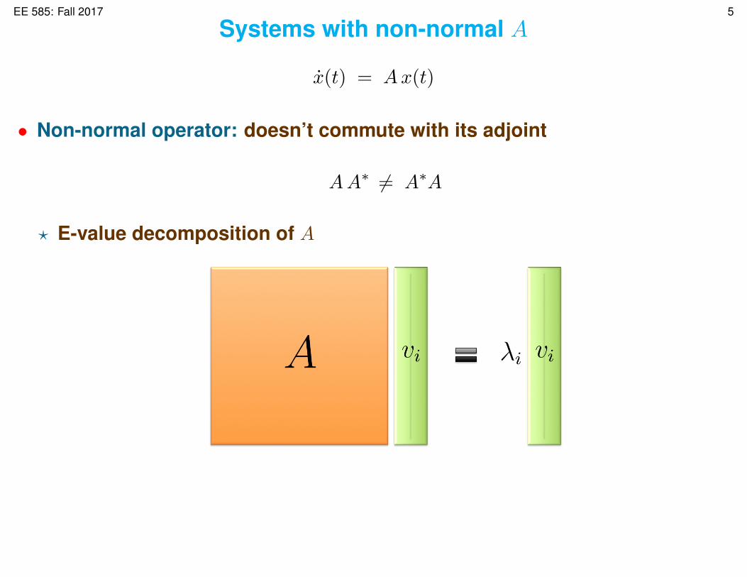
Systems with non-normal A

x(t) = Ax(t)

• Non-normal operator: doesn’t commute with its adjoint

AA∗ 6= A∗A

? E-value decomposition of A

EE 585: Fall 2017 6

• Let A have a full set of linearly independent e-vectors

? normal A: unitarily diagonalizable

A = V ΛV ∗

EE 585: Fall 2017 7

• E-value decomposition of A∗

choose wi such that w∗i vj = δij

EE 585: Fall 2017 8

• Use V and W ∗ to diagonalize A

? solution to x(t) = Ax(t)

x(t) = eA t x(0) =

n∑i=1

eλit vi (wi∗x(0))

EE 585: Fall 2017 9

• Right e-vectors

? identify initial conditions with simple responses

x(t) =

n∑i=1

eλit (wi∗x(0)) vi

y x(0) = vk

x(t) = eλkt vk

EE 585: Fall 2017 10

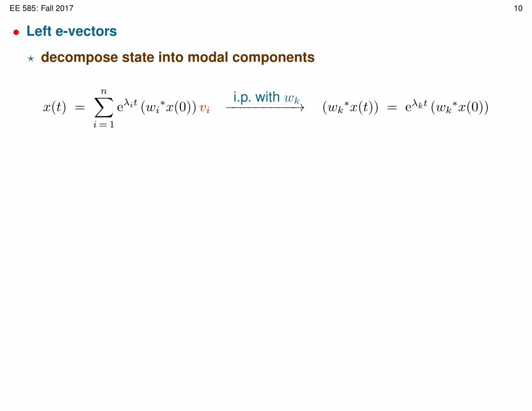
• Left e-vectors

? decompose state into modal components

x(t) =

n∑i=1

eλit (wi∗x(0)) vi

i.p. with wk−−−−−−−−−→ (wk∗x(t)) = eλkt (wk

∗x(0))

EE 585: Fall 2017 11

A toy example[x1x2

]=

[−1 0

k −2

] [x1x2

]

x1(t

),x

2(t

)

EE 585: Fall 2017 12

• E-value decomposition of A =

[−1 0

k −2

]{v1 =

1√1 + k2

[1k

], v2 =

[01

]}{w1 =

[ √1 + k2

0

], w2 =

[−k1

]}

solution to x(t) = Ax(t):

x(t) =(e−t v1w

∗1 + e−2t v2w

∗2

)x(0)

←−[

x1(t)

x2(t)

]=

[e−t x1(0)

k(e−t − e−2t

)x1(0) + e−2t x2(0)

]

• E-values: misleading measures of transient response

EE 585: Fall 2017 13

FORCED RESPONSES(LATER IN THE COURSE)

EE 585: Fall 2017 14

Amplification of disturbances

• Harmonic forcing

d(t) = d(ω) ejωtsteady-state response−−−−−−−−−−−−−−−−−−−→ y(t) = y(ω) ejωt

? Frequency response

y(ω) = C (jωI − A)−1B︸ ︷︷ ︸

H(ω)

d(ω)

example: 3 inputs, 2 outputs

[y1(ω)y2(ω)

]=

[H11(ω) H12(ω) H13(ω)H21(ω) H22(ω) H23(ω)

] d1(ω)

d2(ω)

d3(ω)

Hij(ω) – response from jth input to ith output

EE 585: Fall 2017 15

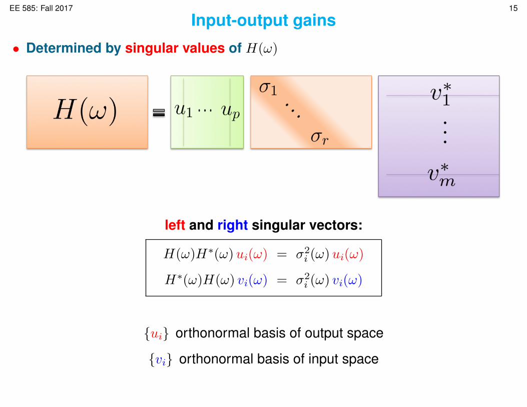
Input-output gains

• Determined by singular values of H(ω)

left and right singular vectors:

H(ω)H∗(ω)ui(ω) = σ2i (ω)ui(ω)

H∗(ω)H(ω) vi(ω) = σ2i (ω) vi(ω)

{ui} orthonormal basis of output space

{vi} orthonormal basis of input space

EE 585: Fall 2017 16

• Action of H(ω) on d(ω)

y(ω) = H(ω) d(ω) =

r∑i=1

σi(ω)ui(ω)⟨vi(ω), d(ω)

⟩

• Right singular vectors

? identify input directions with simple responses

σ1(ω) ≥ σ2(ω) ≥ · · · > 0

y(ω) =r∑

i=1

σi(ω)ui(ω)⟨vi(ω), d(ω)

⟩y d(ω) = vk(ω)

y(ω) = σk(ω)uk(ω)

σ1(ω): the largest amplification at any frequency

EE 585: Fall 2017 17

Worst case amplification• H∞ norm: an induced L2 gain (of a system)

G = ‖H‖2∞ = maxoutput energyinput energy

= maxω

σ21 (H(ω))

σ2 1(H

(ω))

EE 585: Fall 2017 18

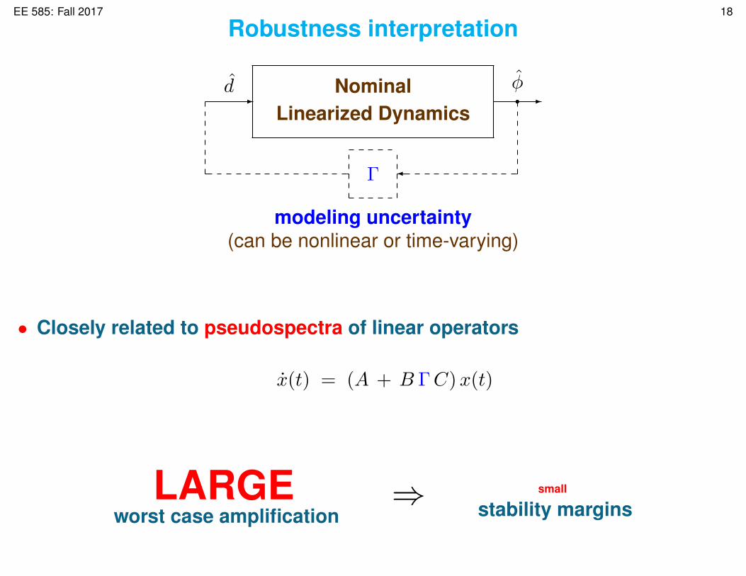
Robustness interpretation

-d Nominal

Linearized Dynamicss -

φ

�Γ

modeling uncertainty(can be nonlinear or time-varying)

• Closely related to pseudospectra of linear operators

x(t) = (A + B ΓC)x(t)

LARGEworst case amplification

⇒ small

stability margins

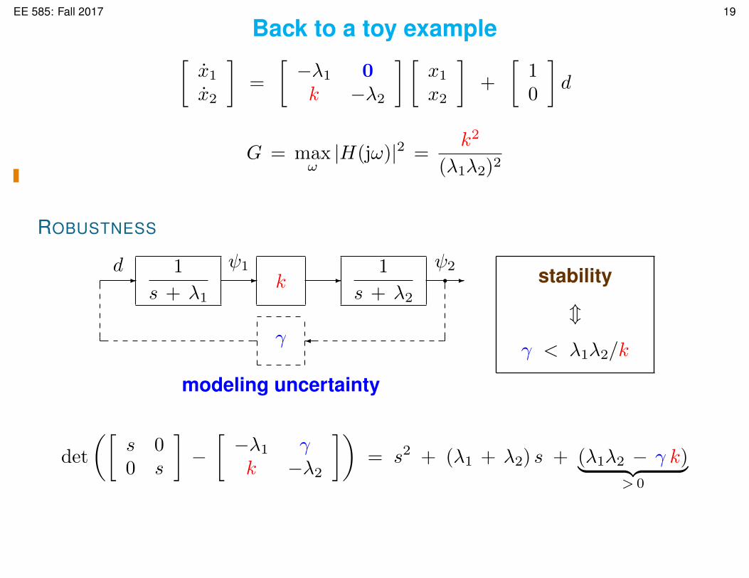
EE 585: Fall 2017 19

Back to a toy example[x1x2

]=

[−λ1 0k −λ2

] [x1x2

]+

[10

]d

G = maxω|H(jω)|2 =

k2

(λ1λ2)2

ROBUSTNESS

-d 1

s + λ1-

ψ1

k -1

s + λ2s -ψ2

�γ

modeling uncertainty

stability

m

γ < λ1λ2/k

det

([s 00 s

]−[−λ1 γk −λ2

])= s2 + (λ1 + λ2) s + (λ1λ2 − γ k)︸ ︷︷ ︸

> 0

EE 585: Fall 2017 20

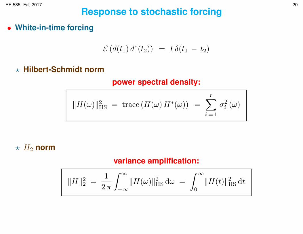
Response to stochastic forcing

• White-in-time forcing

E (d(t1) d∗(t2)) = I δ(t1 − t2)

? Hilbert-Schmidt norm

power spectral density:

‖H(ω)‖2HS = trace (H(ω)H∗(ω)) =

r∑i=1

σ2i (ω)

? H2 norm

variance amplification:

‖H‖22 =1

2π

∫ ∞−∞‖H(ω)‖2HS dω =

∫ ∞0

‖H(t)‖2HS dt

EE 585: Fall 2017 21

Computation of H2 and H∞ norms

x(t) = Ax(t) + B d(t)

y(t) = C x(t)

• H2 norm

? Lyapunov equation

E (d(t1) d∗(t2)) = W δ(t1 − t2) ⇒

{‖H‖22 = trace (C P C∗)

AP + P A∗ = −BWB∗

• H∞ norm

? E-value decomposition of Hamiltonian in conjunction with bisection

‖H‖∞ ≥ γ ⇔

[A 1

γ BB∗

−1γ C∗C −A∗

]has at least one imaginary e-value