model for the swiss reserve market - eth z · the topic of this master thesis originates from the...
TRANSCRIPT

eeh power systemslaboratory
Haoyuan Qu
Three-Stage Stochastic Market-ClearingModel for the Swiss Reserve Market
Master ThesisPSL 1519
Department:EEH – Power Systems Laboratory, ETH Zurich
In collaboration with Swissgrid Ltd
Examiner:Prof. Dr. Goran Andersson, ETH Zurich
Supervisor:Farzaneh Abbaspourtorbati, Swissgrid
Line Roald, ETH ZurichDr. Marek Zima, Swissgrid
Zurich, December 16, 2015

ii

Abstract
The topic of this master thesis originates from the reserve procurement pro-cess in Switzerland. Currently, a two-stage reserve market has been oper-ated where secondary control reserves are procured in a weekly auction andtertiary control reserves are split between weekly and daily auctions. In or-der to make use of additional available power from producers and to allowthe participation of Renewable Energy Sources (RES), a third market stagewhich is closer to real-time operation is likely to be established in the future,converting the reserve procurement process into a three-stage problem.
The chief objective of this master thesis is to develop a three-stagestochastic market-clearing model for the Swiss reserve market. Within theframework of this thesis, scenarios for daily market are scrutinized and im-proved, which can be readily appended to the current two-stage stochasticmarket-clearing model. Scenarios for the third stage are generated based onreference data in the current market and various cases are simulated. Sim-ulation results show that both improvements on the two-stage model andthe incorporation of an additional third stage could lead to cost savings forTransmission System Operator (TSO).
iii

iv

Acknowledgements
This thesis is the outcome of research work done in cooperation betweenPower Systems Laboratory (PSL) at ETH and Swissgrid. After six monthsof efforts, it concludes my master’s studies in Energy Science and Technol-ogy at ETH and is one of the most important milestones in my life.
First, I would like to express my gratitude towards Prof. Dr. Goran Ander-sson for being my tutor and enabling this collaboration with Swissgrid.
My profound thanks go to Dr. Marek Zima, who has provided me withthe opportunity of conducting research at Swissgrid and introduced me tothe fascinating world of ancillary services market.
Furthermore, I would like to give my deepest appreciation to my supervisorat PSL, Line Roald and my supervisor at Swissgrid, Farzaneh Abbaspour-torbati. Without their continuous support and valuable input, I would nothave managed to come to this final stage.
I should not forget to thank my colleagues from Swissgrid who providedme with all sorts of support, be it technically or spiritually.
Last but not least, I would like to thank and share this piece of work withmy beloved family and friends for their lasting love, patience and support.
Zurich, December 2015
Haoyuan
v

vi

Contents
List of Figures x
List of Tables xi
List of Acronyms xiii
List of Symbols xv
1 Introduction 1
1.1 Balancing Reserves . . . . . . . . . . . . . . . . . . . . . . . . 1
1.2 Reserve Market . . . . . . . . . . . . . . . . . . . . . . . . . . 2
1.3 Stochastic Programming . . . . . . . . . . . . . . . . . . . . . 3
1.4 Structure of the Thesis . . . . . . . . . . . . . . . . . . . . . . 5
2 Reserve Market in Switzerland 7
2.1 Self-scheduling Market . . . . . . . . . . . . . . . . . . . . . . 7
2.2 Overview of Ancillary Services . . . . . . . . . . . . . . . . . 8
2.3 Structure of Reserve Market . . . . . . . . . . . . . . . . . . . 11
2.3.1 Primary Control Reserves . . . . . . . . . . . . . . . . 11
2.3.2 Secondary and Tertiary Control Reserves . . . . . . . 12
2.4 Bid Structure . . . . . . . . . . . . . . . . . . . . . . . . . . . 13
2.4.1 Indivisible Bids . . . . . . . . . . . . . . . . . . . . . . 14
2.4.2 Conditional Bids . . . . . . . . . . . . . . . . . . . . . 15
2.5 Dimensioning Criteria . . . . . . . . . . . . . . . . . . . . . . 15
2.5.1 Probabilistic Approach . . . . . . . . . . . . . . . . . . 16
2.5.2 Deterministic Approach . . . . . . . . . . . . . . . . . 17
2.6 Remuneration Scheme . . . . . . . . . . . . . . . . . . . . . . 17
2.6.1 Remuneration of Capacity . . . . . . . . . . . . . . . . 17
2.6.2 Remuneration of Energy . . . . . . . . . . . . . . . . . 17
3 Two-Stage Market-Clearing Model 19
3.1 Background . . . . . . . . . . . . . . . . . . . . . . . . . . . . 19
3.2 Stochastic Market-Clearing Model . . . . . . . . . . . . . . . 20
3.2.1 Decision Variables . . . . . . . . . . . . . . . . . . . . 21
vii

viii CONTENTS
3.2.2 Objective Function . . . . . . . . . . . . . . . . . . . . 223.2.3 Constraints . . . . . . . . . . . . . . . . . . . . . . . . 263.2.4 Formulation . . . . . . . . . . . . . . . . . . . . . . . . 31
3.3 Improvements of Two-Stage Model . . . . . . . . . . . . . . . 323.3.1 Linearization of Bid Curves . . . . . . . . . . . . . . . 323.3.2 Selection of Scenarios . . . . . . . . . . . . . . . . . . 37
4 Three-Stage Market-Clearing Model 454.1 Introduction . . . . . . . . . . . . . . . . . . . . . . . . . . . . 454.2 Stochastic Market-Clearing Model . . . . . . . . . . . . . . . 47
4.2.1 Decision Variables . . . . . . . . . . . . . . . . . . . . 474.2.2 Objective Function . . . . . . . . . . . . . . . . . . . . 474.2.3 Non-anticipativity Matrix . . . . . . . . . . . . . . . . 504.2.4 Constraints . . . . . . . . . . . . . . . . . . . . . . . . 524.2.5 Formulation . . . . . . . . . . . . . . . . . . . . . . . . 53
4.3 Scenarios for Hourly Market . . . . . . . . . . . . . . . . . . . 554.3.1 Modelling of Hourly Bid Curves . . . . . . . . . . . . 554.3.2 Scenario Construction . . . . . . . . . . . . . . . . . . 56
4.4 Simulation Results . . . . . . . . . . . . . . . . . . . . . . . . 584.4.1 Case Study: Impact of Hourly Market . . . . . . . . . 584.4.2 Complete Scenario Simulations . . . . . . . . . . . . . 61
5 Conclusions and Outlook 675.1 Summary . . . . . . . . . . . . . . . . . . . . . . . . . . . . . 675.2 Future Work . . . . . . . . . . . . . . . . . . . . . . . . . . . 68
A Hourly Discretizing Factors 69
Bibliography 71

List of Figures
1.1 Real-time electricity consumption and demand forecast ofNovember 16, 2015 [1] . . . . . . . . . . . . . . . . . . . . . . 2
1.2 Example of a scenario tree for three-stage problems . . . . . . 4
2.1 Temporal structure of frequency control after a disturbance [2] 8
2.2 Simplified diagram of Swiss ancillary services market [3] . . . 11
2.3 Scheme of a two-stage reserve market in Switzerland [4] . . . 12
2.4 Example of SCR and TCR provision . . . . . . . . . . . . . . 14
2.5 Deficit curves for dimensioning reserves in Switzerland [4] . . 16
3.1 Two-stage stochastic market-clearing scheme . . . . . . . . . 20
3.2 Example of a bid curve (before and after linearization) . . . . 24
3.3 Example of piecewise linearized deficit curve . . . . . . . . . . 28
3.4 Overview of bid curve linearization methods . . . . . . . . . . 33
3.5 Example of bid curve linearization by four methods . . . . . . 34
3.6 Residual of fitted bid curve . . . . . . . . . . . . . . . . . . . 35
3.7 Amount of procured reserves using four fitting methods . . . 36
3.8 Total procurement cost of reserves using four fitting methods 36
3.9 Procurement cost in daily market using four fitting methodsafter fixing weekly decision . . . . . . . . . . . . . . . . . . . 36
3.10 Overview of scenario selection methods . . . . . . . . . . . . . 40
3.11 Cost difference w.r.t. perfect information scenario . . . . . . . 41
3.12 Cost difference w.r.t. perfect information scenario (Methods2, 5 and 6) . . . . . . . . . . . . . . . . . . . . . . . . . . . . 42
4.1 Three-stage stochastic market-clearing scheme . . . . . . . . . 46
4.2 Hypothetical hourly bid curve . . . . . . . . . . . . . . . . . . 48
4.3 Free TCE+ volume in 2015 (Week 01−35) . . . . . . . . . . . 56
4.4 Free TCE− volume in 2015 (Week 01−35) . . . . . . . . . . . 56
4.5 Scenario construction process . . . . . . . . . . . . . . . . . . 57
4.6 Definition of cases . . . . . . . . . . . . . . . . . . . . . . . . 59
4.7 Amount of reserves procured for Week 35 2015 . . . . . . . . 60
4.8 Amount of reserves procured for Week 04 2015 . . . . . . . . 60
4.9 Estimated cost savings w.r.t two-stage model . . . . . . . . . 62
ix

x LIST OF FIGURES
4.10 Scenario tree of complete model . . . . . . . . . . . . . . . . . 624.11 Reserve amount of complete model . . . . . . . . . . . . . . . 644.12 Substitution between TCR+ and TCR− products . . . . . . 664.13 Substitution between daily and hourly products . . . . . . . . 66
List of Tables
2.1 Volume of PCR Cooperation in 2015 [5] . . . . . . . . . . . . 112.2 Bid structure of the Swiss reserve market [5] . . . . . . . . . . 132.3 Example bids for demonstration of indivisibility . . . . . . . . 152.4 Example of conditional bids . . . . . . . . . . . . . . . . . . . 152.5 Remuneration of activated SCR [5] . . . . . . . . . . . . . . . 18
3.1 Performance of linearization methods . . . . . . . . . . . . . . 353.2 Estimation of cost savings by improved linearization method
(Week 02−35, 2015) . . . . . . . . . . . . . . . . . . . . . . . 373.3 Explanation of week names . . . . . . . . . . . . . . . . . . . 383.4 Correlation coefficients between weeks . . . . . . . . . . . . . 383.5 RMSE between weeks [CHF/MW] . . . . . . . . . . . . . . . 393.6 Information of selected weeks [6] . . . . . . . . . . . . . . . . 413.7 Comparison of Methods 2, 5 and 6 w.r.t. perfect information 423.8 Estimation of savings by improved scenario selection method
(Week 02−35, 2015) . . . . . . . . . . . . . . . . . . . . . . . 433.9 Estimation of savings by implementing both improvements
(Week 02−35, 2015) . . . . . . . . . . . . . . . . . . . . . . . 43
4.1 Probability factors of hourly scenarios . . . . . . . . . . . . . 584.2 Potential cost savings w.r.t. two-stage model . . . . . . . . . 614.3 Scenario notations . . . . . . . . . . . . . . . . . . . . . . . . 624.4 Problem size . . . . . . . . . . . . . . . . . . . . . . . . . . . 634.5 Amount of reserves procured in complete model . . . . . . . . 644.6 Total cost of procurement of complete model . . . . . . . . . 65
A.1 Hourly discretizing factors . . . . . . . . . . . . . . . . . . . . 70
xi

xii LIST OF TABLES

List of Acronyms
TSO Transmission System OperatorENTSO-E European Network of Transmission System Operators for ElectricityAS Ancillary ServicesBG Balance GroupPCR Primary Control ReservesSCR Secondary Control ReservesTCR Tertiary Control ReservesFCR Frequency Containment ReservesFRR Frequency Restoration ReservesaFRR automatic Frequency Restoration ReservesmFRR manual Frequency Restoration ReservesRR Replacement ReservesAGC Automatic Generation ControlLFC Load Frequency ControlACE Area Control ErrorRES Renewable Energy SourcesMEAS Mutual Emergency Assistance ServiceTCE Tertiary Control EnergyMOL Merit Order ListCDF Cumulative Distribution FunctionMILP Mixed Integer Linear ProgrammingRMSE Root Mean Square Error
xiii

xiv LIST OF ACRONYMS

List of Symbols
xw Decision variable vector of bids in weekly marketxwS Decision variable vector of SCR bids in weekly marketxwT+ Decision variable vector of TCR+ bids in weekly marketxwT− Decision variable vector of TCR− bids in weekly marketxd Decision variable vector of reserve procurement in daily marketxdT+ Vector of TCR+ procurement amount in daily marketxdT− Vector of TCR− procurement amount in daily marketxh Decision variable vector of reserve procurement in hourly marketxhT+ Vector of TCR+ procurement amount in hourly marketxhT− Vector of TCR− procurement amount in hourly market
ωd Index of scenarios for daily marketωh Index of scenarios for hourly marketΩd Scenario set for daily marketΩh Scenario set for hourly marketπd(ωd) Probability of daily scenario ωd
πh(ωh) Probability of hourly scenario ωh
cw Cost vector of bids in weekly marketλT+(ωd) Cost vector of TCR+ in daily market for scenario ωd
λT−(ωd) Cost vector of TCR− in daily market for scenario ωd
ζT+(ωd, ωh) Cost vector of TCR+ in hourly market for scenario combination (ωd, ωh)ζT−(ωd, ωh) Cost vector of TCR− in hourly market for scenario combination (ωd, ωh)
α+i Slope of ith piece of linearized daily bid curve for TCR+
α−i Slope of ith piece of linearized daily bid curve for TCR−β+i Intercept of ith piece of linearized daily bid curve for TCR+β−i Intercept of ith piece of linearized daily bid curve for TCR−
xv
xvi LIST OF SYMBOLS
ρ+i Slope of ith piece of linearized hourly bid curve for TCR+ρ−i Slope of ith piece of linearized hourly bid curve for TCR−ϕ+
i Intercept of ith piece of linearized hourly bid curve forTCR+
ϕ−i Intercept of ith piece of linearized hourly bid curve forTCR−
a(i)s+ Slope of ith piece of linearized deficit curve for secondary
positive reserves
a(i)s− Slope of ith piece of linearized deficit curve for secondary
negative reserves
a(i)o+ Slope of ith piece of linearized deficit curve for overall posi-
tive reserves
a(i)o− Slope of ith piece of linearized deficit curve for overall neg-
ative reserves
b(i)s+ Intercept of ith piece of linearized deficit curve for secondary
positive reserves
b(i)s− Intercept of ith piece of linearized deficit curve for secondary
negative reserves
b(i)o+ Intercept of ith piece of linearized deficit curve for overall
positive reserves
b(i)o− Intercept of ith piece of linearized deficit curve for overall
negative reservesεs+ Probability of deficit of secondary positive reservesεs− Probability of deficit of secondary negative reservesεo+ Probability of deficit of overall positive reservesεo− Probability of deficit of overall negative reserves
xmind,T+(ωd) Lower bound of daily TCR+ procurement amount for daily
scenario ωd
xmaxd,T+(ωd) Upper bound of daily TCR+ procurement amount for daily
scenario ωd
xmind,T−(ωd) Lower bound of daily TCR− procurement amount for daily
scenario ωd
xmaxd,T−(ωd) Upper bound of daily TCR− procurement amount for daily
scenario ωd
xminh,T+(ωh) Lower bound of hourly TCR+ procurement amount for
hourly scenario ωh
xmaxh,T+(ωh) Upper bound of hourly TCR+ procurement amount for
hourly scenario ωh
xminh,T−(ωh) Lower bound of hourly TCR− procurement amount for
hourly scenario ωh
xmaxh,T−(ωh) Upper bound of hourly TCR− procurement amount for
hourly scenario ωh

Chapter 1
Introduction
This chapter unveils the background of this thesis. Key concepts involved arebalancing reserves and market for reserve procurement. Stochastic program-ming, the core methodology applied in this thesis, will be briefly introducedin Section 1.3. The framework of this thesis is then exhibited in Section 1.4.
1.1 Balancing Reserves
Power systems operate at a certain frequency, e.g. 50 Hz in Europe and amajority of countries in the world, and 60 Hz in the Americas and part ofAsia. It is important to maintain system frequency within a small range ofdeviation. On the one hand, large frequency deviations can damage equip-ment and affect load performance. On the other hand, if frequency dropstoo much, generation units might be disconnected from the grid by protec-tion devices, further enlarging frequency deviation. In worst cases, largefrequency fluctuations could possibly lead to interruption of power supplyand system collapse [7].
In most European countries, Transmission System Operators (TSOs)are responsible for the security of transmission system and coordinating thesupply of and demand for electrical energy to avoid frequency deviations.Generally, a surplus in generation shifts system frequency upwards, whilea deficit depresses it [7]. Therefore, in order to maintain constant systemfrequency, production and consumption of electricity have to be balancedinstantaneously and continuously.
However, demand forecast can never yield 100% precision. Forecast er-rors, sudden load changes and unforeseen generation incidents can causepower imbalances between supply and demand in the system. Under thecircumstances, TSOs have to deploy balancing energy to “fill the gap” be-tween supply and demand. Yet one of the most unique features of electricalenergy is that it cannot be stored. In order to ensure that there is sufficientenergy in real-time operation for the purpose of balancing, TSOs usually
1
2 CHAPTER 1. INTRODUCTION
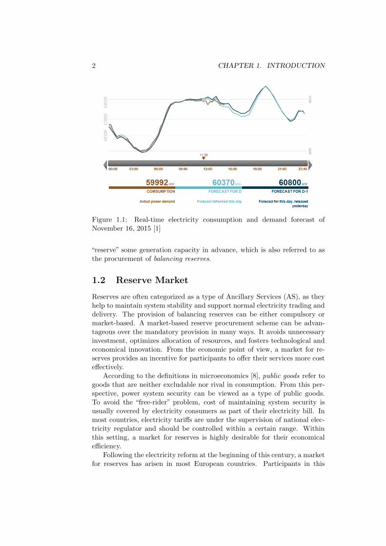
Figure 1.1: Real-time electricity consumption and demand forecast ofNovember 16, 2015 [1]
“reserve” some generation capacity in advance, which is also referred to asthe procurement of balancing reserves.
1.2 Reserve Market
Reserves are often categorized as a type of Ancillary Services (AS), as theyhelp to maintain system stability and support normal electricity trading anddelivery. The provision of balancing reserves can be either compulsory ormarket-based. A market-based reserve procurement scheme can be advan-tageous over the mandatory provision in many ways. It avoids unnecessaryinvestment, optimizes allocation of resources, and fosters technological andeconomical innovation. From the economic point of view, a market for re-serves provides an incentive for participants to offer their services more costeffectively.
According to the definitions in microeconomics [8], public goods refer togoods that are neither excludable nor rival in consumption. From this per-spective, power system security can be viewed as a type of public goods.To avoid the “free-rider” problem, cost of maintaining system security isusually covered by electricity consumers as part of their electricity bill. Inmost countries, electricity tariffs are under the supervision of national elec-tricity regulator and should be controlled within a certain range. Withinthis setting, a market for reserves is highly desirable for their economicalefficiency.
Following the electricity reform at the beginning of this century, a marketfor reserves has arisen in most European countries. Participants in this
1.3. STOCHASTIC PROGRAMMING 3
market can be pre-qualified power plants, industrial consumers or possiblysomeone providing demand side response. TSOs are normally the sole buyerin this market. The demand is determined by dimensioning criteria set byENTSO-E and TSO. Depending on different market setup, providers withaccepted bids are reimbursed either at their bid price (pay-as-bid) or theprice of the last accepted bid (market-clearing price).
The operation of reserve market is usually separated into two steps: di-mensioning and procurement. Traditionally, TSOs complete these two stepsin a sequential order, i.e. first determine the demand using dimensioningcriteria and then procure the fixed amount in the market. In Germany,for example, reserves are dimensioned using probabilistic criteria and thenecessary amount is published every three months for the next quarter [9].Afterwards, a tender auction process for the fixed demand will take place,in which bids with the most attractive offering price will be awarded.
While this traditional approach obeys the security criteria, it neglectsthe temporal coupling between different market stages and potential sub-stitution between different types of reserves by unlinking dimensioning andprocurement [4], which results in overly conservative procurement decisions.In [4], a new market-clearing approach for reserve market is proposed. Thisnew approach is a two-stage stochastic market-clearing model based on thestructure of the Swiss reserve market and has been implemented since Jan-uary 2014. The economic saving of this new approach is estimated to bearound 12 million Swiss francs (CHF) in 2014.
1.3 Stochastic Programming
Stochastic programming is a model for optimization under uncertainty. Ingeneral, stochastic programming incorporates a wide range of problems: two-stage recourse problems, multi-stage stochastic problems, stochastic integerprograms, chance-constrained programs, etc. [10], of which the first one ismost widely studied and applied. This thesis is based on a two-stage recourseproblem, and extends it to a three-stage stochastic problem.
In a two-stage or three-stage stochastic programming problem, multipledecisions are made as we progress in time, with more information on theunknown parameter being disclosed. Here, uncertainty is represented by afinite number of input data, which can be random variables or stochasticprocesses. The objective function is formulated as the sum of individualsolutions of each set of input data weighted by the corresponding probabilityfactor. Hence, instead of optimizing deterministic objective functions, theexpected value of objective function (if not risk-averse) is optimized. Thefinal solution is therefore the best solution for all sets of input data, but notfor each individual scenario particularly [11].
Some common terminologies in stochastic programming are explained
4 CHAPTER 1. INTRODUCTION
below [10,11]:
• Stage: a point in time where a new decision has to be made with achange in uncertainty.
• Here-and-now decisions: decisions made without any realization ofuncertain information.
• Wait-and-see decisions: decisions made after uncertainty has totallyor partially unfolded.
• Recourse action: additional actions possible in second or further stageswhen uncertainty reveals.
• Scenarios: a set of data representing stochastic processes spanninga given time horizon. For instance, if λ is the hourly electricityprice of next week (168 hours), λ can be represented by NΩ scenariosλ(1), · · · ,λ(ω), · · · ,λ(NΩ), each with a length of 168×1 and occurringwith a probability of π(ω), where ω is the scenario index.
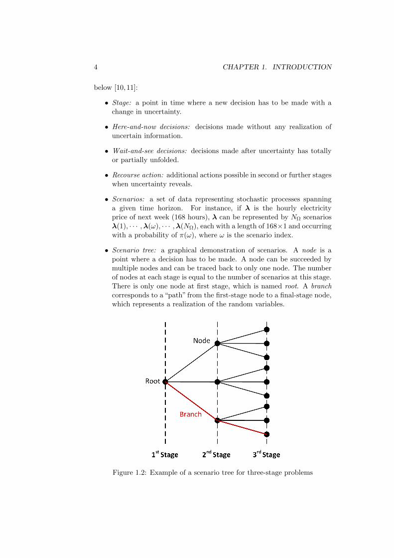
• Scenario tree: a graphical demonstration of scenarios. A node is apoint where a decision has to be made. A node can be succeeded bymultiple nodes and can be traced back to only one node. The numberof nodes at each stage is equal to the number of scenarios at this stage.There is only one node at first stage, which is named root. A branchcorresponds to a “path” from the first-stage node to a final-stage node,which represents a realization of the random variables.
Figure 1.2: Example of a scenario tree for three-stage problems
1.4. STRUCTURE OF THE THESIS 5
In recent years, there has been a growing trend of real-world applicationsof stochastic programming. Examples are especially concentrated in thefields of finance and energy [12]. The application of three-stage stochasticprogramming in electricity market is generally focused on maximizing theprofits of power producers in multi-stage trading activities [13–15]. Researchon reserve market-clearing using stochastic programming models is mostlyconducted under the setting of a centralized market where reserve and energyare jointly cleared [16,17]. These approaches are, however, not applicable forthe market design in Europe, where energy trading is separated from reservemarket operation. To our knowledge, Swiss reserve market is one of the onlyreal-world implementations of a stochastic market-clearing model reportedso far [4]. The idea of further extending it to a three-stage stochastic market-clearing model is thus novel as well.
1.4 Structure of the Thesis
The main objective of this thesis is to develop a three-stage stochasticmarket-clearing model for the Swiss reserve market. This market-clearingmodel can be adapted to future reserve market design in Switzerland, wherepower plants may be requested to offer all or part of their remaining genera-tion capacity close to real-time for the purpose of balancing. An alternativeapplication can be based on current market design in situations where plentyof balancing energy bids are received without a priori accepted reserve bids.
The contributions of this thesis are twofold:
1. Scenarios for current two-stage stochastic market-clearing model areinvestigated and improved, mainly from the aspects of scenario mod-elling and scenario selection method. The improvements are simulatedwith real market data and can be readily implemented in current Swissreserve market.
2. A three-stage stochastic market-clearing model for Swiss reserve mar-ket is proposed, which is so far novel in applications of stochasticprogramming. Based on analysis of current market reference data,scenarios for third stage are created in order to simulate possibilitiesin future Swiss reserve market.
Therefore, the thesis is organized as follows:Chapter 2 opens with an overview of ancillary services in Switzerland
and the organization of their procurement. The focus is then shifted to themarket design of secondary and tertiary control reserves. Explanations onbid structure, dimensioning criteria and remuneration scheme follow.
Chapter 3 presents the current two-stage stochastic market-clearing model.Formulation of the model is depicted in Section 3.2, while Section 3.3 ex-hibits improvements on scenarios used in the two-stage model.

6 CHAPTER 1. INTRODUCTION
In Chapter 4, formulation of the three-stage stochastic market-clearingmodel is illustrated, followed by explanations on modelling and selectionmethod of third-stage scenarios in Section 4.3. Then, simulations regardingthe three-stage model are run and results are presented.
Chapter 5 covers the conclusion and the outlook of this project.

Chapter 2
Reserve Market inSwitzerland
In this chapter, the Swiss ancillary services market is presented. The focuswill be specially on the procurement of frequency control reserves. Marketstructure, bid structure, dimensioning criteria and remuneration scheme ofreserve market will be explained in Sections 2.3, 2.4, 2.5 and 2.6 respectively.
2.1 Self-scheduling Market
In most European countries, wholesale trading of electricity is separatedfrom dispatch by TSOs. This type of market design is named self-schedulingmarket, or decentralized market, as opposed to centralized market in NorthAmerica. Switzerland belongs to one of these countries.
In a self-scheduling market, generation schedule of each power plant isdetermined on their own based on their economic interest. In most cases,these schedules are based on results from bilateral, day-ahead and intradaypower trading. Schedules are submitted to TSOs after trading closes. TSOswill only intervene when there is a need for balancing or when securitycriteria are violated. In such cases, TSO will deploy Ancillary Services (AS)to ensure system security and reliability.
In Switzerland, connection between energy markets and TSO (Swissgrid)is established through Balance Group (BG) model [18]. A balance group isa virtual aggregation of several feed-in and feed-out points. Energy transac-tions are carried out by each BG as an entity. After transaction closes, BGsare obliged to deliver their schedules to Swissgrid. Meanwhile, Swissgridbalances the production and consumption within the entire Swiss network.However, due to forecast errors and inexacts, actual delivery of energy islikely to deviate from schedules, creating imbalances in the system (a.k.a.balance energy). The settlement of balance energy is a two-price systemdepending on the direction of discrepancy. The prices are usually unfavor-
7
8 CHAPTER 2. RESERVE MARKET IN SWITZERLAND
able to BGs as a measure to discourage such discrepancies. Formula forcalculating imbalance settlement price can be found in [18]. The prices arecalculated by Swissgrid and posted on Swissgrid’s website every month.
2.2 Overview of Ancillary Services
As national TSO, Swissgrid guarantees the secure and reliable operation ofpower system with the help of ancillary services from providers. Ancillaryservices organized by Swissgrid primarily include frequency control, volt-age support, compensation of active power losses and black start [3], whichare explained below. The main focus of this thesis is on frequency controlreserves.
Frequency Control
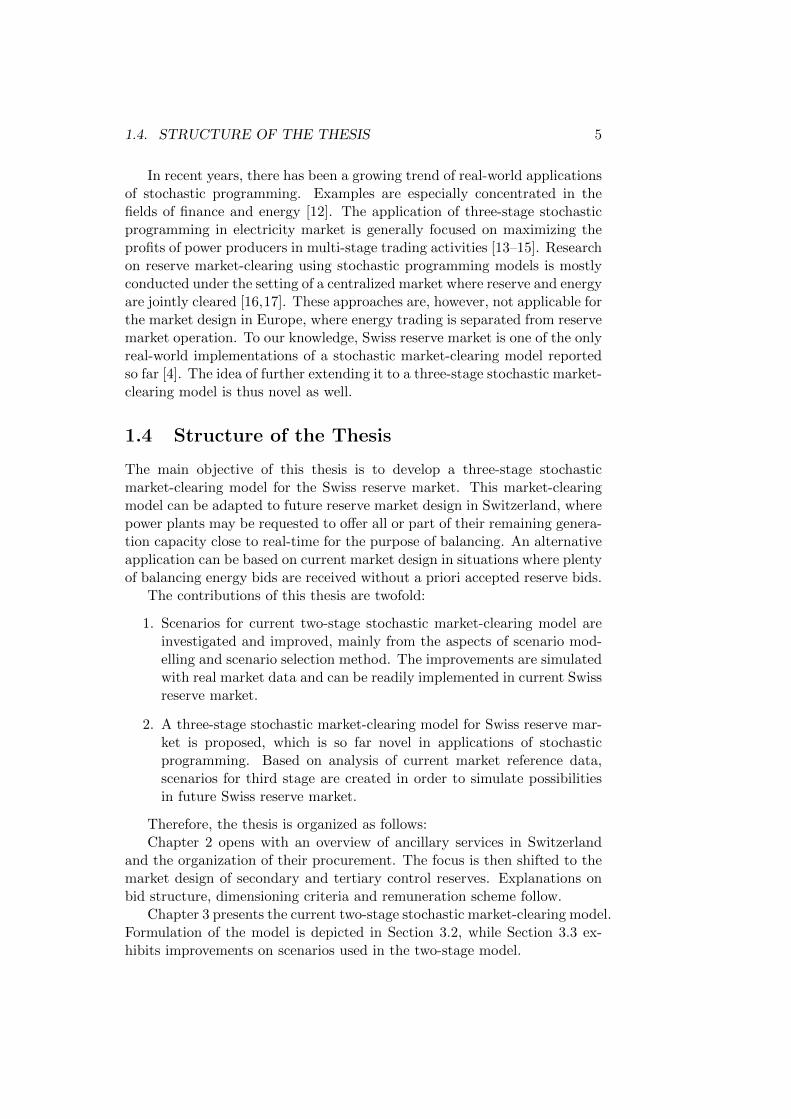
Frequency control can also be referred to as active power control, whereimbalances between electricity production and consumption are balancedby deploying control reserves. According to European Network of Transmis-sion System Operators for Electricity (ENTSO-E), system frequency controlcan be divided into three levels: primary control, secondary control and ter-tiary control [19]. Correspondingly, three types of frequency control reservesare defined: Primary Control Reserves (PCR), Secondary Control Reserves(SCR) and Tertiary Control Reserves (TCR). In [20], the conventional termsare replaced by modern terms of control reserves. In this thesis, conventionalterms of reserves will be kept since they are still more familiar to audiencein the industry nowadays. Figure 2.1 presents the activation sequence ofthe three types of frequency control. Technical features of the three-levelfrequency control are summarized as follows.
Figure 2.1: Temporal structure of frequency control after a disturbance [2]

2.2. OVERVIEW OF ANCILLARY SERVICES 9
1. Primary Frequency ControlThe purpose of primary frequency control is mainly to stabilize systemfrequency after a disturbance at steady state. Full activation time isusually 30 seconds after disturbance in Continental Europe [21]. Pri-mary frequency control is activated through automatically adjustingsetpoints for frequency and power at a local generator and is thereforedecentralized control. Since this type of control is purely proportional,it merely prevents system frequency from further deviating, but can-not restore frequency to normal value. All online generators shouldbe technically available for the provision of primary frequency controlthrough installation of speed governors [2]. Some frequency sensitiveloads such as induction motors also participate in this control by coun-teracting frequency deviations [22,23].Primary control reserves are also known as Frequency ContainmentReserves (FCR). In the synchronous area of Continental Europe, theoverall amount of primary control reserve is 3000 MW [19]. Thisamount is shared between member states and the demand in eachcountry is designated by European Network of Transmission SystemOperators for Electricity (ENTSO-E) every year.
2. Secondary Frequency ControlSecondary frequency control is also referred to as Automatic Gener-ation Control (AGC) or Load Frequency Control (LFC). Secondarycontrol is activated to restore system frequency and power exchangesbetween areas in case of frequency noises under normal operation or af-ter a large incident. The activation of secondary control usually starts30 seconds after the disturbance and is completed within 15 minutesat the latest [19]. In contrast with primary control, secondary controlcan be regarded as a type of centralized control. However, only gen-erators in the control area where frequency disturbance occurred willparticipate in this control.In modern terms of ENTSO-E, secondary control reserves are cate-gorized into Frequency Restoration Reserves (FRR), or more specif-ically, automatic Frequency Replacement Reserves (aFRR), as somedocuments indicate [24]. Secondary control reserves can also releaseprimary control reserves as they can sustain for longer periods.
3. Tertiary Control ReservesThe purpose of tertiary control is usually twofold: to assist secondarycontrol reserve to recover system frequency and to replace primaryand secondary control reserves. The activation of tertiary frequencycontrol is manual, in the forms of calls from local TSO. After receiving
10 CHAPTER 2. RESERVE MARKET IN SWITZERLAND
the activation signal, power plant operators will adjust the setpointvalues of power output manually. In some countries, tertiary controlis also activated for the purpose of managing congested lines, which isoften referred to as re-dispatch.According to modern ENTSO-E definitions, fast tertiary control re-serves (those can be fully activated within 15 minutes) are groupedinto Frequency Restoration Reserves (FRR), or more specifically man-ual Frequency Restoration Reserves (mFRR), while slower units par-ticipate as Replacement Reserves (RR) (activation time can be from15 minutes up to 1 hour).
Voltage Support
In power systems analysis, voltage at each node is usually coupled with theexchange of reactive power. Maintaining certain voltage level is also crucialin system operation, since large deviations will cause damages to electri-cal equipment and further jeopardize system security. Therefore, as TSO,Swissgrid should ensure that voltage at each node remains in an acceptablerange.
Voltage support is mainly realized by reactive power control. Unlikeactive power, reactive power cannot be transmitted. Thus, reactive powercontrol is rather local [2].
So far, there is no tendering process for reactive power in Switzerland.All power stations online must provide a certain volume of reactive powerin order to keep the voltage within the range indicated by Swissgrid. Theexchanged reactive energy is remunerated at a fixed rate (CHF/Mvarh) [25].
Compensation of Active Power Losses
Resistance in power transmission lines inevitably leads to losses of activepower. These energy losses must be compensated in the network in order todeliver the desired amount of energy to end-consumers. In Switzerland, thetendering process for active power losses and inadvertent deviations takesplace once per month. Any balance group in the Swiss control area can par-ticipate and compensated energy will be remunerated at its bid price basedon exchange schedules [5].
Black Start and Island Operation
Black start refers to the ability of power generators to start operating with-out the need for power injection from the grid. Island operation is thecapability of a power station to operate continuously without requiring anyconnection to the synchronous grid. Both services are guarantees for the
2.3. STRUCTURE OF RESERVE MARKET 11
restoration of power grid after large incidents. Currently, the provision ofblack start and island operation services is secured via bilateral agreementbetween the provider and Swissgrid [25].
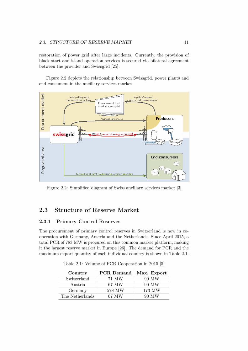
Figure 2.2 depicts the relationship between Swissgrid, power plants andend consumers in the ancillary services market.
Figure 2.2: Simplified diagram of Swiss ancillary services market [3]
2.3 Structure of Reserve Market
2.3.1 Primary Control Reserves
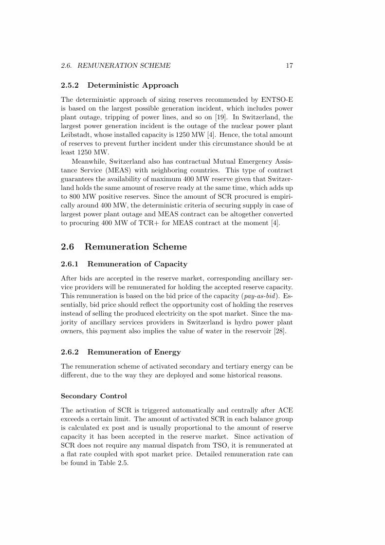
The procurement of primary control reserves in Switzerland is now in co-operation with Germany, Austria and the Netherlands. Since April 2015, atotal PCR of 783 MW is procured on this common market platform, makingit the largest reserve market in Europe [26]. The demand for PCR and themaximum export quantity of each individual country is shown in Table 2.1.
Table 2.1: Volume of PCR Cooperation in 2015 [5]
Country PCR Demand Max. Export
Switzerland 71 MW 90 MW
Austria 67 MW 90 MW
Germany 578 MW 173 MW
The Netherlands 67 MW 90 MW

12 CHAPTER 2. RESERVE MARKET IN SWITZERLAND
In this common market, power plants from all four countries can submittheir bids into the pool. The tender call takes place every Tuesday afternoon[26]. After gate closure, the market will be cleared and those bids with lowestprice will be accepted, regardless of their geographical location (providedthat the maximum export quantity of each country is not exceeded). Theprocured PCR will be utilized across the four participating countries.
2.3.2 Secondary and Tertiary Control Reserves
SCR and TCR are procured together in a national reserve market in Switzer-land. This reserve market is the main focus of this thesis.
Currently, SCR is procured on a weekly basis, whereas the procurementof TCR is split between a weekly auction and daily auction. Figure 2.3illustrates the scheme of the two-stage Swiss reserve market.
Figure 2.3: Scheme of a two-stage reserve market in Switzerland [4]
Weekly Market
The weekly auction for SCR and TCR is closed every Tuesday afternoonat 13:00 [27], before the gate closure of PCR market. At this stage, ASproviders who are willing to participate in this market will submit their bidsfor SCR and/or TCR into system. The bids in the weekly market must bevalid for a horizon of the whole week, i.e. 168 hours.
2.4. BID STRUCTURE 13
Daily Market
TCR can also be procured from a daily market, which provides power plantswith more flexibility. In a daily market, there are six auctions, each of themcomprising a 4-hour block. Power plants can bid for any of these blocks.Accepted bids must be available for a duration of 4 hours.
Traditionally, the share of reserves in the weekly and daily market is de-termined prior to the tender call. However, this approach does not allow anyflexibility in the amount procured in weekly and daily market, hence leadingto higher procurement costs. The stochastic approach, on the other hand,takes into account options from both markets and finds the optimal solution,i.e. the procurement combination with the lowest cost. This approach willbe elaborated in Section 3.2.
2.4 Bid Structure
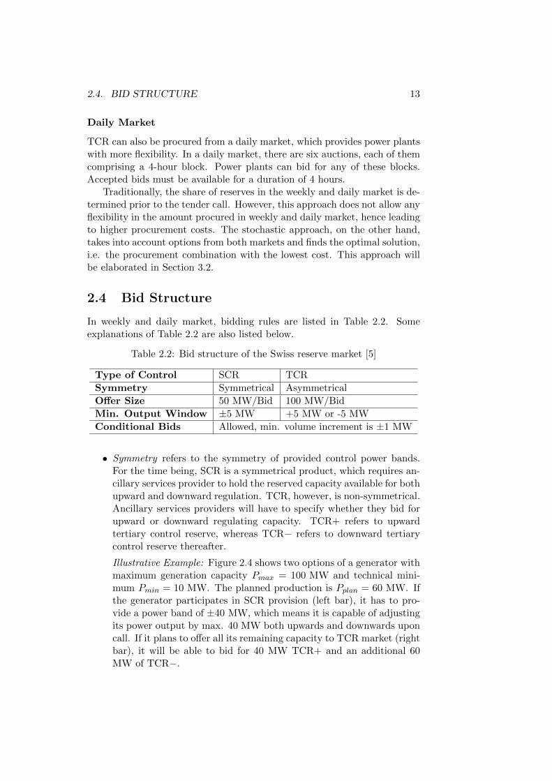
In weekly and daily market, bidding rules are listed in Table 2.2. Someexplanations of Table 2.2 are also listed below.
Table 2.2: Bid structure of the Swiss reserve market [5]
Type of Control SCR TCR
Symmetry Symmetrical Asymmetrical
Offer Size 50 MW/Bid 100 MW/Bid
Min. Output Window ±5 MW +5 MW or -5 MW
Conditional Bids Allowed, min. volume increment is ±1 MW
• Symmetry refers to the symmetry of provided control power bands.For the time being, SCR is a symmetrical product, which requires an-cillary services provider to hold the reserved capacity available for bothupward and downward regulation. TCR, however, is non-symmetrical.Ancillary services providers will have to specify whether they bid forupward or downward regulating capacity. TCR+ refers to upwardtertiary control reserve, whereas TCR− refers to downward tertiarycontrol reserve thereafter.
Illustrative Example: Figure 2.4 shows two options of a generator withmaximum generation capacity Pmax = 100 MW and technical mini-mum Pmin = 10 MW. The planned production is Pplan = 60 MW. Ifthe generator participates in SCR provision (left bar), it has to pro-vide a power band of ±40 MW, which means it is capable of adjustingits power output by max. 40 MW both upwards and downwards uponcall. If it plans to offer all its remaining capacity to TCR market (rightbar), it will be able to bid for 40 MW TCR+ and an additional 60MW of TCR−.

14 CHAPTER 2. RESERVE MARKET IN SWITZERLAND
Figure 2.4: Example of SCR and TCR provision
• Offer Size means the maximum volume of a bid.
• Minimum Output Window is namely the minimum volume of each bid.
• Conditional Bids are bids which allow different price/volume combi-nations. Minimum volume increment is the resolution of these combi-nations. More details will be explained in Section 2.4.2.
2.4.1 Indivisible Bids
In current design of Swiss reserve market, bids are not divisible. This meansthat a bid can either be rejected or accepted. There is no such result thata bid is partially accepted or split. As a result, decision variables for eachindividual bid are binary variables as such:
ξ(i) =
1, bid i is accepted
0, bid i is rejected
Illustrative Example: Assume that there are four bids in the pool and totaldemand for reserve capacity is 100 MW.
In this illustrative example, if we select bids purely based on the meritorder of bid prices, Bids #1 and #2 will be selected. Since Bid #2 cannotbe split to match the total demand, the total cost in this case will be:50 × 5 + 70 × 6 = 670 CHF. Instead, if bids #1 and #3 are accepted, thetotal cost will be: 50× 5 + 50× 7 = 600 CHF.
Therefore, from the perspective of minimizing total cost, the secondcombination of Bids (#1 and #3) is more favorable than the first (#1 and#2), although the unit price of Bid #2 is lower than Bid #3.
2.5. DIMENSIONING CRITERIA 15
Table 2.3: Example bids for demonstration of indivisibility
Bid #Volume
[MW]Price
[CHF/MW]
1 50 5
2 70 6
3 50 7
4 80 8
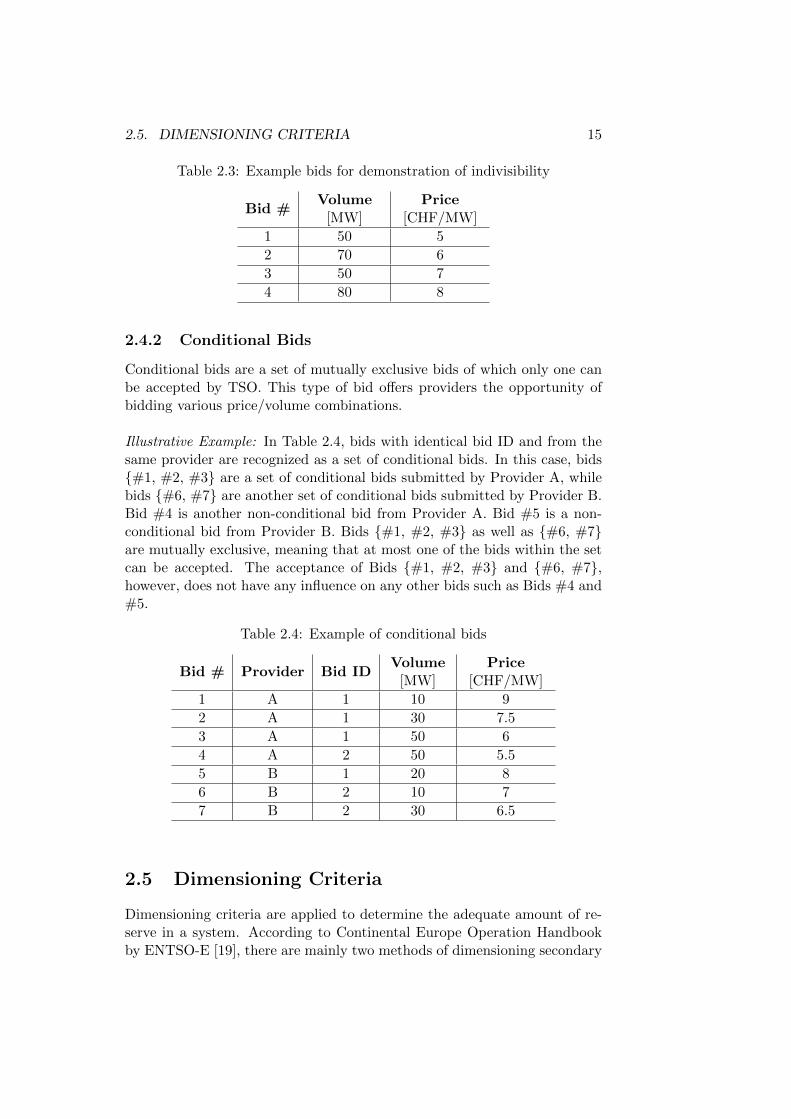
2.4.2 Conditional Bids
Conditional bids are a set of mutually exclusive bids of which only one canbe accepted by TSO. This type of bid offers providers the opportunity ofbidding various price/volume combinations.
Illustrative Example: In Table 2.4, bids with identical bid ID and from thesame provider are recognized as a set of conditional bids. In this case, bids#1, #2, #3 are a set of conditional bids submitted by Provider A, whilebids #6, #7 are another set of conditional bids submitted by Provider B.Bid #4 is another non-conditional bid from Provider A. Bid #5 is a non-conditional bid from Provider B. Bids #1, #2, #3 as well as #6, #7are mutually exclusive, meaning that at most one of the bids within the setcan be accepted. The acceptance of Bids #1, #2, #3 and #6, #7,however, does not have any influence on any other bids such as Bids #4 and#5.
Table 2.4: Example of conditional bids
Bid # Provider Bid IDVolume
[MW]Price
[CHF/MW]
1 A 1 10 9
2 A 1 30 7.5
3 A 1 50 6
4 A 2 50 5.5
5 B 1 20 8
6 B 2 10 7
7 B 2 30 6.5
2.5 Dimensioning Criteria
Dimensioning criteria are applied to determine the adequate amount of re-serve in a system. According to Continental Europe Operation Handbookby ENTSO-E [19], there are mainly two methods of dimensioning secondary

16 CHAPTER 2. RESERVE MARKET IN SWITZERLAND
and tertiary control reserves: probabilistic approach and deterministic ap-proach. In Switzerland, criteria for dimensioning reserves are a hybrid ofprobabilistic and deterministic approach [4].
2.5.1 Probabilistic Approach
The probabilistic approach of dimensioning reserves is based on the rec-ommendation by ENTSO-E that the Area Control Error (ACE) has to beregulated to zero in a certain amount of hours within a year [19]. The per-centage of hours is not strictly specified by ENTSO-E and can be determinedby each TSO individually. Switzerland, for example, requires that ACE shallbe smoothened to zero in 99.8% of all hours during a year. In other words,the deficit of reserves should not occur with a probability of more than0.2% [4], which can also be interpreted as the deficit rate of reserves.
To determine the deficit rate of reserves, cumulative probability distribu-tion curves of power imbalances (deficit curve) are used. The deficit curvenormally takes into account all possible causes of failures, forecast errorsand fluctuations of Renewable Energy Sources (RES).
In Switzerland, two sets of deficit curves are built with respect to thedimensioning of secondary reserves solely and total amount of secondaryand tertiary reserves respectively. For the former curve, AGC signals andremaining ACE are aggregated to form spontaneous power imbalance ∆Ps,which is expected to be compensated by secondary reserves. The latter curveconsiders AGC signals, remaining ACE as well as activated tertiary reserves,which yields to the so-called open-loop ACE, or overall power imbalance ∆Po.This open-loop ACE will be covered by the sum of secondary and tertiarycontrol reserves. Figure 2.5 demonstrates the deficit curves for dimensioningsecondary and overall reserve amount in Switzerland.
Figure 2.5: Deficit curves for dimensioning reserves in Switzerland [4]
2.6. REMUNERATION SCHEME 17
2.5.2 Deterministic Approach
The deterministic approach of sizing reserves recommended by ENTSO-Eis based on the largest possible generation incident, which includes powerplant outage, tripping of power lines, and so on [19]. In Switzerland, thelargest power generation incident is the outage of the nuclear power plantLeibstadt, whose installed capacity is 1250 MW [4]. Hence, the total amountof reserves to prevent further incident under this circumstance should be atleast 1250 MW.
Meanwhile, Switzerland also has contractual Mutual Emergency Assis-tance Service (MEAS) with neighboring countries. This type of contractguarantees the availability of maximum 400 MW reserve given that Switzer-land holds the same amount of reserve ready at the same time, which adds upto 800 MW positive reserves. Since the amount of SCR procured is empiri-cally around 400 MW, the deterministic criteria of securing supply in case oflargest power plant outage and MEAS contract can be altogether convertedto procuring 400 MW of TCR+ for MEAS contract at the moment [4].
2.6 Remuneration Scheme
2.6.1 Remuneration of Capacity
After bids are accepted in the reserve market, corresponding ancillary ser-vice providers will be remunerated for holding the accepted reserve capacity.This remuneration is based on the bid price of the capacity (pay-as-bid). Es-sentially, bid price should reflect the opportunity cost of holding the reservesinstead of selling the produced electricity on the spot market. Since the ma-jority of ancillary services providers in Switzerland is hydro power plantowners, this payment also implies the value of water in the reservoir [28].
2.6.2 Remuneration of Energy
The remuneration scheme of activated secondary and tertiary energy can bedifferent, due to the way they are deployed and some historical reasons.
Secondary Control
The activation of SCR is triggered automatically and centrally after ACEexceeds a certain limit. The amount of activated SCR in each balance groupis calculated ex post and is usually proportional to the amount of reservecapacity it has been accepted in the reserve market. Since activation ofSCR does not require any manual dispatch from TSO, it is remunerated ata flat rate coupled with spot market price. Detailed remuneration rate canbe found in Table 2.5.

18 CHAPTER 2. RESERVE MARKET IN SWITZERLAND
Table 2.5: Remuneration of activated SCR [5]
Direction Upward Downward
Price SwissIXa +20%b SwissIX −20%c
Cash Flow Swissgrid → Bidder Bidder → Swissgrid
Energy Flow Bidder → Swissgrid Swissgrid → Bidder
aHourly price index for Swiss day-ahead auction in EPEX Spot Marketbat least weekly basecat most weekly base
Tertiary Control
In contrast with SCR, TCR is deployed manually. When a dispatcher in shiftobserves continuous power imbalance that needs to be balanced, he/she willmanually call ancillary services providers to activate their tertiary control.The lead time is currently 15 minutes in Switzerland.
For this reason, an separate market for Tertiary Control Energy (TCE)arises to allow ancillary services providers to bid for the regulating energythey provide. Providers with TCR bids accepted in the reserve market mustsubmit energy bids to TCE market. Apart from compulsory bids, additionalenergy can also be offered voluntarily without previously accepted reservebids [5]. Dispatchers will activate TCE based on demand and Merit OrderList (MOL). Bids with lowest price will be activated first. Currently, pay-ment of activated tertiary energy is calculated based on activated amountand bid price.

Chapter 3
Two-Stage Market-ClearingModel
This chapter focuses on the current two-stage stochastic market-clearingmodel and the formulation of the model. Contributions of this thesis areinvestigation and improvement of second-stage scenarios used in this two-stage model. These improvements result in higher accuracy of predictingbidding behavior in daily market using historical data and thus decrease to-tal procurement cost.
3.1 Background
As is briefly stated in Sections 1.2 and 2.3, traditional reserve procure-ment process decouples dimensioning from procurement and neglects thelink between weekly and daily market. By introducing a two-stage stochas-tic market-clearing model, dimensioning and procurement are coupled, andsubstitution between weekly and daily products is also enabled. The chiefobjective is to minimize total expected procurement cost while respectingall constraints.
Figure 3.1 illustrates the decision-making model of this two-stage mar-ket. Weekly market is cleared once per week. At this point in time, adecision on the procurement in weekly market has to be made with onlyweekly bids available. It is still uncertain how market participants will bidin daily market. Unknown daily bids are therefore modelled by a finitenumber of scenarios, each representing a possible set of inputs with a givenprobability. Based on these daily scenarios and known bids from the weeklyauction, weekly procurement decision is made with regard to weekly bids tobe accepted and suggested amount of reserve to be procured in daily mar-ket. After the two-stage clearing of weekly market, results are then passedonto the daily market, where daily bids are received. At this stage, a de-terministic market-clearing process is carried out with actual daily bids and
19

20 CHAPTER 3. TWO-STAGE MARKET-CLEARING MODEL
Figure 3.1: Two-stage stochastic market-clearing scheme
procurement results from previous stage.In the context of this thesis, first stage refers to weekly market, and
second stage refers to daily market. In this chapter, only the two-stagestochastic model for weekly market clearing will be elaborated. The deter-ministic clearing model for daily market is a simple optimization problembased on given bids.
3.2 Stochastic Market-Clearing Model
This section will introduce the formulation of the two-stage stochastic pro-gramming model for current reserve market. The objective of this opti-mization problem is to minimize expected total cost of procurement of allscenarios. Constraints include bidding behavior of known market stages,probabilistic and deterministic dimensioning criteria, etc. An overview ofthe optimization model is presented in Equation (3.1).
min expected total procurement cost
s.t. conditional bids in weekly marketprobabilistic dimensioning criteriadeterministic dimensioning criteria
(3.1)
Please note that bids are usually submitted by BGs (portfolio-based)instead of a specific power plant (unit-based). Thus, this model does notinclude any power flow and power balance equations. The selection of bidsis purely based on bid price and bid volume.
Components of this optimization problem will be built step by step inSections 3.2.1, 3.2.2 and 3.2.3. The complete model will be presented againas a whole in Section 3.2.4.

3.2. STOCHASTIC MARKET-CLEARING MODEL 21
3.2.1 Decision Variables
In this two-stage stochastic programming problem, there are two differentdecision variable vectors, each representing a stage.
First-Stage Decision Variables
Considering different products in the weekly reserve market, the decisionvariable vector of first stage consists of three components:
xw = [xwS ,x
wT+,xw
T− ], (3.2)
where
• xw ∈ ΥNw×1 is the decision variable vector of bids in weekly market
• xwS ∈ ΥNw
S ×1 is the decision variable vector of SCR bids in weeklymarket
• xwT+∈ Υ
NwT+×1
is the decision variable vector of TCR+ bids in weeklymarket
• xwT−∈ ΥNw
T−×1 is the decision variable vector of TCR− bids in weeklymarket
• Υ = 0, 1 is the set of binary variables indicating acceptance andrejection of a bid
• NwS is the number of SCR weekly bids
• NwT+
is the number of TCR+ weekly bids
• NwT−
is the number of TCR− weekly bids
• Nw = NwS + Nw
T++ Nw
T−is the total number of bids in the weekly
market (including SCR, TCR+ and TCR−)
As real bids from the weekly market are considered in this model, theindivisibility of bids should preserved in the decision-making process. Thisfeature can be interpreted as binary decision variables for weekly bids, as isalready discussed in Section 2.4.1.
In case of conditional bids, each single bid within the set of conditionalbids will still be counted as one bid and is assigned with a binary variable.An additional constraint is added to ensure the property of conditional bids,which will be explained in Section 3.2.3.

22 CHAPTER 3. TWO-STAGE MARKET-CLEARING MODEL
Second-Stage Decision Variables
In the second stage, a finite number of scenarios are constructed in orderto model the uncertainty. For each daily scenario ωd, an individual second-stage decision variable vector xd(ωd) is assigned:
xd(ωd) = [xdT+
(ωd),xdT−(ωd)], (3.3)
where
• ωd ∈ Ωd is the index of scenarios for daily market
• Ωd contains NdΩ scenarios for daily market
• xdT+
(ωd) ∈ R42×1 is the amount of TCR+ to be procured in daily
market in each 4-hour time block for scenario ωd
• xdT−
(ωd) ∈ R42×1 is the amount of TCR− to be procured in the daily
market in each 4-hour time block for scenario ωd
In the second stage, TCR market is cleared for each 4-hour time block.Since the results from two-stage market clearing are valid for one week (24×7 = 168 hours), length of second-stage parameters and variables is often168/4 = 42, which corresponds to 42 time blocks in a week.
3.2.2 Objective Function
The objective of this optimization model is to minimize expected procure-ment cost. The total cost can be calculated as the sum of first-stage cost(deterministic cost of weekly market) and second-stage cost (expected valueof daily costs with respect to different scenarios):
min Λw + E[Λd(ωd)],
∀ωd ∈ Ωd,(3.4)
where Λw is the total procurement cost in the weekly market and Λd(ωd)is the total procurement cost in the daily market for the given week withinput data of scenario ωd. E[Λd(ωd)] is the expectation of daily procurementcosts in all scenarios.
First-Stage Cost Function
Since the first stage of this problem is deterministic, cost incurred in theweekly market is calculated as the cumulative cost of accepted bids:
Λw = cᵀwxw = (κ · p)ᵀxw (3.5)
where

3.2. STOCHASTIC MARKET-CLEARING MODEL 23
• cw ∈ RNw×1 is the cost vector of all weekly bids
• κ ∈ RNw×1 is a vector containing unit prices (CHF/MW) of each bid
• p ∈ RNw×1 = [pS ,pT+ ,pT− ] is a vector consisting of volume (MW) ofeach bid
• pS is a vector consisting of volume (MW) of each SCR bid
• pT+ is a vector consisting of volume (MW) of each TCR+ bid
• pT− is a vector consisting of volume (MW) of each TCR− bid
Second-Stage Cost Function
To render the computation time affordable for real market clearing, thisstochastic programming problem is limited to a Mixed Integer Linear Pro-gramming (MILP) problem. Therefore, all components are to be linearized.To model daily costs, bid curves are derived from actual bids and then lin-earized via the following steps:
1. For each 4-hour time block, bids are obtained for TCR+ and TCR−respectively.
2. As for conditional bids, the bid with minimum price within the set isselected to represent this set. If there are multiple bids with the sameminimum price, the one with the largest quantity is chosen.
3. Bids are sorted in ascending order according to their bid prices.
4. Cumulative volume and cost are calculated respectively.
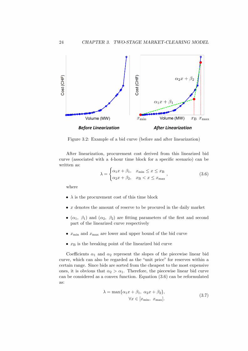
5. A bid curve is drawn based on cumulative volume and cost. Theleft curve in Figure 3.2 shows an example of bid curve. Each bluecircle represents a bid. The x-coordinate corresponds to the cumulativevolume up to this bid, whereas the y-coordinate is the cumulative costfor such volume.
6. To incorporate daily bids into the linear model, bid curves are lin-earized. The curve on the right in Figure 3.2 depicts how a bid curve(blue line) can be approximated by two straight lines (green dashedlines).
Two-piece linearization is selected by the current market-clearing algo-rithm, since it represents bidding behavior in a most efficient manner.
24 CHAPTER 3. TWO-STAGE MARKET-CLEARING MODEL
Figure 3.2: Example of a bid curve (before and after linearization)
After linearization, procurement cost derived from this linearized bidcurve (associated with a 4-hour time block for a specific scenario) can bewritten as:
λ =
α1x+ β1, xmin ≤ x ≤ xB
α2x+ β2, xB < x ≤ xmax
, (3.6)
where
• λ is the procurement cost of this time block
• x denotes the amount of reserve to be procured in the daily market
• (α1, β1) and (α2, β2) are fitting parameters of the first and secondpart of the linearized curve respectively
• xmin and xmax are lower and upper bound of the bid curve
• xB is the breaking point of the linearized bid curve
Coefficients α1 and α2 represent the slopes of the piecewise linear bidcurve, which can also be regarded as the “unit price” for reserves within acertain range. Since bids are sorted from the cheapest to the most expensiveones, it is obvious that α2 > α1. Therefore, the piecewise linear bid curvecan be considered as a convex function. Equation (3.6) can be reformulatedas:
λ = maxα1x+ β1, α2x+ β2,∀x ∈ [xmin, xmax].
(3.7)

3.2. STOCHASTIC MARKET-CLEARING MODEL 25
Equation (3.7) can be written as an optimization problem:
minx
λ
s.t. α1x+ β1 ≤ λ,α2x+ β2 ≤ λ,
xmin ≤ x ≤ xmax.
(3.8)
In reality, daily procurement costs are calculated for each 4-hour timeblock and summed up. Fitting parameters α1, α2, β1 and β2 vary accord-ing to each piecewise linear bid curve derived for each time block and areconstructed for each scenario. Therefore, Equation (3.8) can be extended tothe full week horizon and all scenarios in the daily market:
minxdT+
(ωd), xdT−
(ωd)λT+(ωd) + λT−(ωd)
s.t. α+1 (ωd)xd
T+(ωd) + β+
1 (ωd) ≤ λT+(ωd),
α+2 (ωd)xd
T+(ωd) + β+
2 (ωd) ≤ λT+(ωd),
α−1 (ωd)xdT−
(ωd) + β−1 (ωd) ≤ λT−(ωd),
α−2 (ωd)xdT−
(ωd) + β−2 (ωd) ≤ λT−(ωd),
xdT+
(ωd) ∈ [xmind,T+
(ωd), xmaxd,T+
(ωd)],
xdT−
(ωd) ∈ [xmind,T−
(ωd), xmaxd,T−
(ωd)],
∀ωd ∈ Ωd,
(3.9)
where
• λT+(ωd) ∈ R42×1 is the cost vector of TCR+
• λT−(ωd) ∈ R42×1 is the cost vector of TCR−
• α+1 (ωd), β+
1 (ωd), α+2 (ωd), β+
2 (ωd) ∈ R42×1 are fitting parameters ofTCR+ bid curves
• α−1 (ωd), β−1 (ωd), α−2 (ωd), β−2 (ωd) ∈ R42×1 are fitting parameters ofTCR− bid curves
• xmind,T+
(ωd), xmaxd,T+
(ωd) are lower and upper bound of TCR+ bid curve
• xmind,T−
(ωd), xmaxd,T−
(ωd) are lower and upper bound of TCR− bid curve
Therefore, the term E[Λd(ωd)] in the Equation (3.4) can be reformulatedas:
E[Λd(ωd)] =∑
ωd∈Ωd
πd
(ωd) [
11×42λT+(ωd) + 11×42λT−(ωd)],
∀ωd ∈ Ωd,
(3.10)
where πd(ωd)
is the probability of scenario ωd and 11×42 is the summa-tion vector whose elements are all 1.

26 CHAPTER 3. TWO-STAGE MARKET-CLEARING MODEL
3.2.3 Constraints
The constraints considered in the stochastic market-clearing model primarilyencompass three aspects:
1. Conditional bids in weekly market
2. Probabilistic dimensioning criterion
3. Deterministic dimensioning criterion
The mathematical formulation of three types of constraints will be ex-plained individually in this section.
Conditional Bids in Weekly Market
According to current bidding rules in the Swiss reserve market, providersare allowed to submit a set of conditional bids. Definition and example ofconditional bids are given in Section 2.4.2.
To guarantee that this rule will not be violated in the optimization prob-lem, it is translated into the following constraint:
Acxw ≤ bc, (3.11)
where
• Ac ∈ RNwc ×Nw
is a matrix whose element is either 1 or 0 dependingon whether the corresponding bid is within the set of conditional bidsor not
• bc ∈ RNwc ×1 is a vector whose elements are all 1
• Nwc is the number of conditional bid sets amongst all bids in the weekly
market (including SCR, TCR+ and TCR−)
Illustrative Example: Consider the bids in Table 2.4. Bids #1, #2, #3and #6, #7 are two sets of conditional bids. The decision vector for theseseven bids is:
x = [x1, x2, · · · , x7]ᵀ,
where xi ∈ 0, 1 is the binary decision variable for Bid #i.According to the definition of conditional bids, at most one of x1, x2 and
x3 can have a value of 1. The rest should be 0. This is also applicable forx6 and x7. The rule of conditional bids can thus be written as:
x1 + x2 + x3 ≤ 1
x6 + x7 ≤ 1.
In this case, Ac =
[1 1 1 0 0 0 00 0 0 0 0 1 1
], and bc =
[11
].

3.2. STOCHASTIC MARKET-CLEARING MODEL 27
Probabilistic Dimensioning Criterion
The probabilistic criterion for dimensioning reserves states that the portionof time within a year when secondary control reserve alone is not able tocover spontaneous power imbalances and when secondary and tertiary con-trol reserve together are not able to cover overall power imbalances shouldnot exceed 0.2% [4]. This percentage can be translated as the probability ofpower imbalances being greater than the amount of reserves procured:
P (∆Ps ≥ Rs) + P (∆Po ≥ Ro) ≤ 0.2%, (3.12)
where ∆Ps and ∆Po are spontaneous and overall power imbalances re-spectively, Rs and Ro are the amount of secondary and overall reserves(including SCR and TCR).
Considering both positive and negative power imbalances, Equation (3.12)can be rewritten as:
P(∆Ps+ ≥ Rs+
)+ P
(∆Ps− ≤ −Rs−
)+ P
(∆Po+ ≥ Ro+
)+P(∆Po− ≤ −Ro−
)≤ 0.2%,
(3.13)
where
• ∆Ps+ > 0 and ∆Ps− < 0 are positive and negative spontaneous powerimbalances respectively
• ∆Po+ > 0 and ∆Po− < 0 are positive and negative overall powerimbalances respectively
• Rs+ and Rs− refer to positive and negative SCR (currently in Switzer-land Rs+ = Rs−)
• Ro+ and Ro− refer to overall positive and negative control reserves
If we define cumulative distribution functions of power imbalances assuch:
Fs+(p) = P(∆Ps+ ≥ p
)Fs−(p) = P
(∆Ps− ≤ −p
)Fo+(p) = P
(∆Po+ ≥ p
)Fo−(p) = P
(∆Po− ≤ −p
) , (3.14)
then Equation (3.15) can be reformulated as:
Fs+(Rs+) + Fs−(Rs−) + Fo+(Ro+) + Fo−(Ro−) ≤ 0.002. (3.15)
28 CHAPTER 3. TWO-STAGE MARKET-CLEARING MODEL
The amount of procured reserve Rs+ , Rs− , Ro+ and Ro− can be replacedby decision variables in the following terms:
Rs+ = Rs− = pᵀSxwS ,
Ro+ = pᵀSxwS + pᵀT+
xwT+
+ xdT+
(ωd),
Ro− = pᵀSxwS + pᵀT−
xwT−
+ xdT−
(ωd),
∀ωd ∈ Ωd.
(3.16)
Inserting Equation (3.16) into (3.15), Equation (3.15) becomes:
Fs+(pᵀSxwS ) + Fs−(pᵀSx
wS ) + Fo+
(pᵀSx
wS + pᵀT+
xwT+
+ xdT+
(ωd))
+Fo−
(pᵀSx
wS + pᵀT−
xwT− + xd
T−(ωd))≤ 0.002, ∀ωd ∈ Ωd.
(3.17)
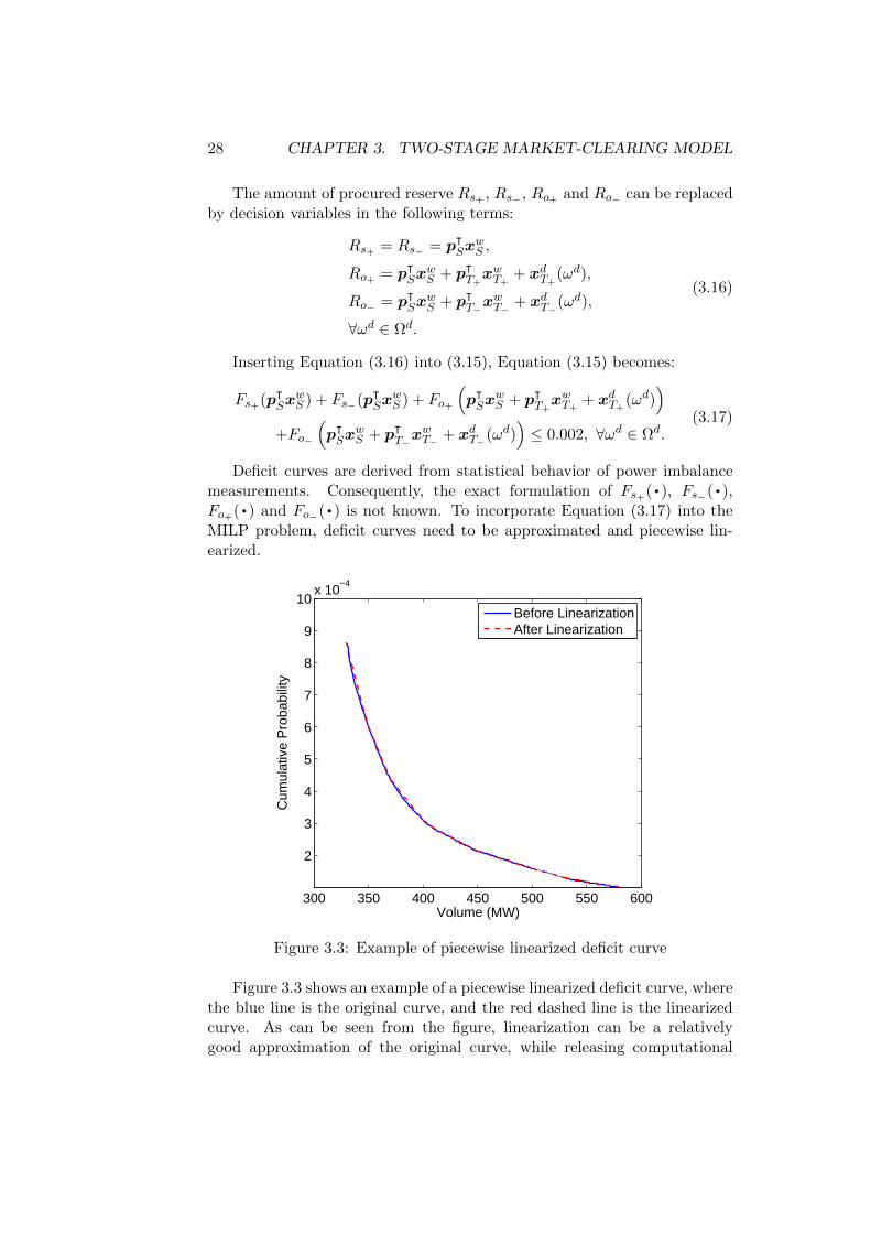
Deficit curves are derived from statistical behavior of power imbalancemeasurements. Consequently, the exact formulation of Fs+(·), Fs−(·),Fo+(·) and Fo−(·) is not known. To incorporate Equation (3.17) into theMILP problem, deficit curves need to be approximated and piecewise lin-earized.
300 350 400 450 500 550 600
2
3
4
5
6
7
8
9
10x 10
−4
Volume (MW)
Cum
ulat
ive
Pro
babi
lity
Before LinearizationAfter Linearization
Figure 3.3: Example of piecewise linearized deficit curve
Figure 3.3 shows an example of a piecewise linearized deficit curve, wherethe blue line is the original curve, and the red dashed line is the linearizedcurve. As can be seen from the figure, linearization can be a relativelygood approximation of the original curve, while releasing computational
3.2. STOCHASTIC MARKET-CLEARING MODEL 29
burden of the problem. The linearization process takes place once per halfa year along with the update of original deficit curve based on the mostrecent measurement data. After linearization, parameters are obtained andinserted into constraints:
εs+ =
a(1)s+Rs+ + b
(1)s+ , Rs+ ∈
[r
(0)s+ , r
(1)s+
]a
(2)s+Rs+ + b
(2)s+ , Rs+ ∈
[r
(1)s+ , r
(2)s+
]...
...
a(m)s+ Rs+ + b
(m)s+ , Rs+ ∈
[r
(m−1)s+ , r
(m)s+
](3.18)
εs− =
a(1)s−Rs− + b
(1)s− , Rs− ∈
[r
(0)s− , r
(1)s−
]a
(2)s−Rs− + b
(2)s− , Rs− ∈
[r
(1)s− , r
(2)s−
]...
...
a(n)s− Rs− + b
(n)s− , Rs− ∈
[r
(n−1)s− , r
(n)s−
](3.19)
εo+ =
a(1)o+Ro+ + b
(1)o+ , Ro+ ∈
[r
(0)o+ , r
(1)o+
]a
(2)o+Ro+ + b
(2)o+ , Ro+ ∈
[r
(1)o+ , r
(2)o+
]...
...
a(j)o+Ro+ + b
(j)o+ , Ro+ ∈
[r
(j−1)o+ , r
(j)o+
](3.20)
εo− =
a(1)o−Ro− + b
(1)o− , Ro− ∈
[r
(0)o− , r
(1)o−
]a
(2)o−Ro− + b
(2)o− , Ro− ∈
[r
(1)o− , r
(2)o−
]...
...
a(k)o−Ro− + b
(k)o− , Ro− ∈
[r
(k−1)o− , r
(k)o−
](3.21)
where
• subscripts s+, s−, o+, o− denote variables/parameters of secondarypositive, secondary negative, overall positive and overall negative re-serves
• ε·(R) is the probability of deficit with a reserve amount of R accordingto the corresponding deficit curve
• a(i)· and b(i)· are linearization parameters of piece i of the corresponding
deficit curve
30 CHAPTER 3. TWO-STAGE MARKET-CLEARING MODEL
• m, n, j, k are the total number of pieces for each linearized deficitcurve
•[r
(i−1)· , r(i)·]
is the range of reserve volume in which linear piece i is
valid
Theoretically, deficit curves should be close to convex functions. Underthis assumption, Equations (3.18)−(3.21) can be treated similarly as thelinearized bid curves in Section 3.2.2. Thus, constraints with respect to theprobabilistic dimensioning criterion can be formulated as:
a(i)s+
(Rs+
)+ b
(i)s+ ≤ εs+ , i = 1, · · · ,m,
a(i)s−
(Rs−
)+ b
(i)s− ≤ εs− , i = 1, · · · , n,
a(i)o+
(Ro+
)+ b
(i)o+ ≤ εo+ , i = 1, · · · , j,
a(i)o−
(Ro−
)+ b
(i)o− ≤ εo− , i = 1, · · · , k,
Rmins+ ≤ Rs+ ≤ Rmax
s+ ,
Rmins− ≤ Rs− ≤ Rmax
s− ,
Rmino+ ≤ Ro+ ≤ Rmax
o+ ,
Rmino− ≤ Ro− ≤ Rmax
o− ,
εs+ + εs− + εo+ + εo− ≤ 0.002.
(3.22)
In this set of constraints, εs+ , εs− , εo+ and εo− are regarded as “deci-sion variables” and appended to those described in Section 3.2.1. They donot appear in objective function, though. Rs+ , Rs− , Ro+ and Ro− can beexpressed by decision variables according to Equation (3.16).
Deterministic Dimensioning Criterion
According to Section 2.5.2, the deterministic criterion of sizing reserves inSwitzerland can be described as a minimum TCR+ of 400 MW according toMEAS contract. This criterion can thus be written with weekly and dailydecision variables as follows:
400 ≤ pᵀT+xwT+
+ xdT+
(ωd),
∀ωd ∈ Ωd.(3.23)
3.2. STOCHASTIC MARKET-CLEARING MODEL 31
3.2.4 Formulation
The complete mathematical formulation of the current two-stage stochasticmarket-clearing model is presented as follows:
minxw, λT+
(ωd), λT− (ωd)cᵀwx
w +∑
ωd∈Ωd
πd
(ωd) [
11×42λT+(ωd) + 11×42λT−(ωd)]
(3.24)
s.t. Acxw ≤ bc, (3.25)
α+1 (ωd)xd
T+(ωd) + β+
1 (ωd) ≤ λT+(ωd), ∀ωd ∈ Ωd,
(3.26)
α+2 (ωd)xd
T+(ωd) + β+
2 (ωd) ≤ λT+(ωd), ∀ωd ∈ Ωd,
(3.27)
α−1 (ωd)xdT−(ωd) + β−1 (ωd) ≤ λT−(ωd), ∀ωd ∈ Ωd,
(3.28)
α−2 (ωd)xdT−(ωd) + β−2 (ωd) ≤ λT−(ωd), ∀ωd ∈ Ωd,
(3.29)
a(i)s+
(pᵀSx
wS
)+ b(i)s+ ≤ εs+ , i = 1, · · · ,m, (3.30)
a(i)s−
(pᵀSx
wS
)+ b(i)s− ≤ εs− , i = 1, · · · , n, (3.31)
a(i)o+
(pᵀSx
wS + pᵀT+
xwT+
+ xdT+
(ωd))
+ b(i)o+ ≤ εo+ ,
∀ωd ∈ Ωd, i = 1, · · · , j, (3.32)
a(i)o−
(pᵀSx
wS + pᵀT−
xwT− + xd
T−(ωd))
+ b(i)o− ≤ εo− ,
∀ωd ∈ Ωd, i = 1, · · · , k, (3.33)
εs+ + εs− + εo+ + εo− ≤ 0.002, (3.34)
400 ≤ pᵀT+xwT+
+ xdT+
(ωd), ∀ωd ∈ Ωd, (3.35)
xdT+
(ωd) ∈ [xmind,T+
(ωd), xmaxd,T+
(ωd)], ∀ωd ∈ Ωd, (3.36)
xdT−(ωd) ∈ [xmin
d,T−(ωd), xmaxd,T−(ωd)], ∀ωd ∈ Ωd. (3.37)
Constraint (3.25) corresponds to the conditional bids received in weeklymarket. Constraints (3.26)−(3.29) are related to piecewise linearized dailybid curves. (3.30)−(3.34) are associated with probabilistic dimensioning cri-terion. Constraint (3.35) is for deterministic dimensioning criterion (MEASconstraint). Last but not least, constraints (3.36) and (3.37) define feasibleranges for daily procurement amounts.

32 CHAPTER 3. TWO-STAGE MARKET-CLEARING MODEL
3.3 Improvements of Two-Stage Model
This section presents two major improvements made to the current two-stage market-clearing model: linearization of bid curves and selection ofdaily scenarios. Different methods are investigated and compared. Resultsshow that cost savings can be achieved with these improvements, which canbe readily implemented in Swissgrid.
3.3.1 Linearization of Bid Curves
The linearization method of bid curves refers to how the piecewise linearizedbid curve in Figure 3.2 is obtained. It encompasses two aspects: the numberof curve pieces and the method of obtaining linearization parameters.
In [4], a two-piece linearization method is applied and this method hasbeen implemented since the launch of two-stage stochastic market-clearingmodel in Switzerland. This linearization method is based on minimizing themaximum fitting error on a curve, which is referred to as maximum errorestimation hereafter.
The process of searching for optimal fitting parameters using maximumerror estimation can be described as:
min γs.t. |yi − yi| ≤ γ,
yi =
α1xi + β1, xi ∈ [x(0)B , x
(1)B ]
...
αjxi + βj , xi ∈ [x(j−1)B , x
(j)B ]
...
αMxi + βM , xi ∈ [x(M−1)B , x
(M)B ]
,
∀i = 1, · · · , N,
(3.38)
where
• (xi, yi) represents an individual bid on bid curve, and xi, yi denotecumulative volume and cost at this point respectively
• yi is the estimated cost after linearization at xi
• N is the total number of data points to be fitted on the bid curve
• γ denotes the maximum error between fitted curve and original curve
• αj and βj are linearization parameters of piece j
• x(j−1)B and x
(j)B indicate the lower and upper bound of piece j
• M is the total number of pieces of the linearized curve

3.3. IMPROVEMENTS OF TWO-STAGE MODEL 33
Another commonly used method in curve fitting is least squares estima-tion. It can be described via the following formulation:
min
N∑i=1
(yi − yi)2
s.t. yi =
α1xi + β1, xi ∈ [x(0)B , x
(1)B ]
...
αjxi + βj , xi ∈ [x(j−1)B , x
(j)B ]
...
αMxi + βM , xi ∈ [x(M−1)B , x
(M)B ]
,
∀i = 1, · · · , N,
(3.39)
Notations in Equation (3.39) follow those in Equation (3.38).
In the linearization process, optimizations based on Equation (3.38) or(3.39) are repeated for each combination of bids taken as breaking point. Theoptimal solution is then the minimum value of objective functions among alliterations.
Sometimes a two-piece linearization of the bid curve can result in in-accurate estimation of daily procurement cost. This usually occurs whenthe shape of bid curve is close to quadratic, for example the one in Figure3.2. In such cases, more pieces should be considered while linearizing thebid curve. However, too many pieces will significantly increase the num-ber of iterations due to more combinations of breaking points. Consideringthe computational burden, the maximum number of curve pieces consideredhere is three.
Therefore, four linearization methods (Figure 3.4) concerning two dimen-sions (number of pieces and estimation method) are analyzed and compared.The number of pieces refer to the value of M in Equations (3.38) and (3.39).
Figure 3.4: Overview of bid curve linearization methods
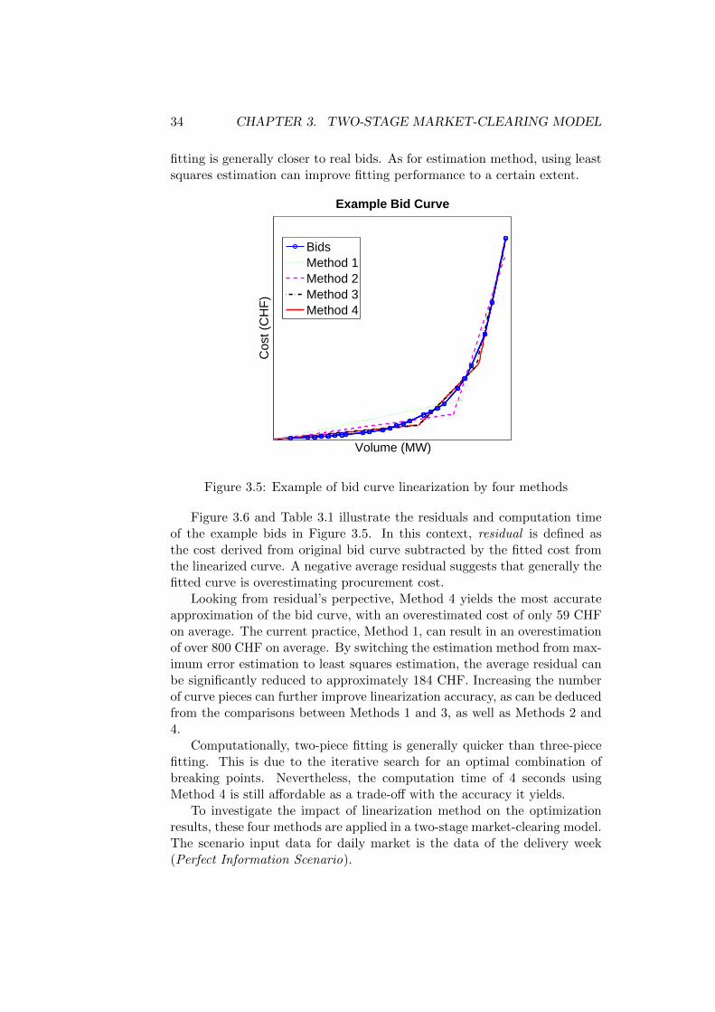
Figure 3.5 shows an example of bid curve linearization using the above-mentioned four different methods. As can be seen from the figure, three-piece
34 CHAPTER 3. TWO-STAGE MARKET-CLEARING MODEL
fitting is generally closer to real bids. As for estimation method, using leastsquares estimation can improve fitting performance to a certain extent.
Volume (MW)
Cos
t (C
HF
)
Example Bid Curve
BidsMethod 1Method 2Method 3Method 4
Figure 3.5: Example of bid curve linearization by four methods
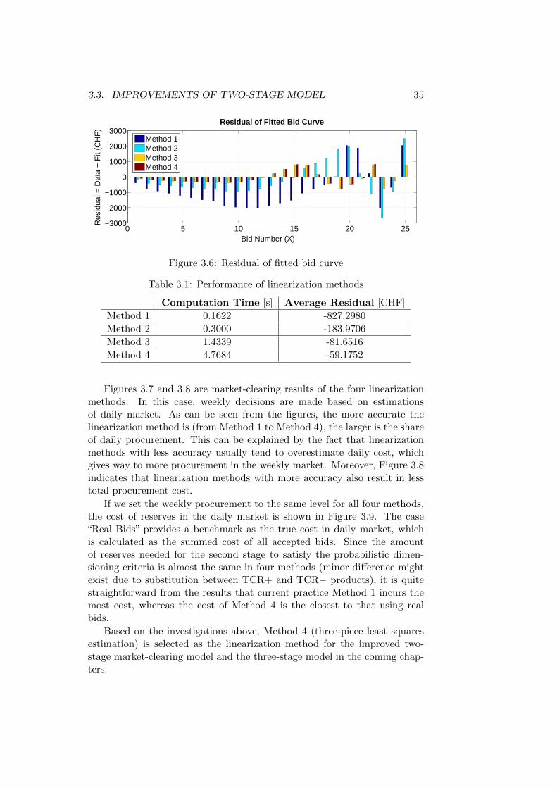
Figure 3.6 and Table 3.1 illustrate the residuals and computation timeof the example bids in Figure 3.5. In this context, residual is defined asthe cost derived from original bid curve subtracted by the fitted cost fromthe linearized curve. A negative average residual suggests that generally thefitted curve is overestimating procurement cost.
Looking from residual’s perpective, Method 4 yields the most accurateapproximation of the bid curve, with an overestimated cost of only 59 CHFon average. The current practice, Method 1, can result in an overestimationof over 800 CHF on average. By switching the estimation method from max-imum error estimation to least squares estimation, the average residual canbe significantly reduced to approximately 184 CHF. Increasing the numberof curve pieces can further improve linearization accuracy, as can be deducedfrom the comparisons between Methods 1 and 3, as well as Methods 2 and4.
Computationally, two-piece fitting is generally quicker than three-piecefitting. This is due to the iterative search for an optimal combination ofbreaking points. Nevertheless, the computation time of 4 seconds usingMethod 4 is still affordable as a trade-off with the accuracy it yields.
To investigate the impact of linearization method on the optimizationresults, these four methods are applied in a two-stage market-clearing model.The scenario input data for daily market is the data of the delivery week(Perfect Information Scenario).
3.3. IMPROVEMENTS OF TWO-STAGE MODEL 35
0 5 10 15 20 25−3000
−2000
−1000
0
1000
2000
3000Residual of Fitted Bid Curve
Bid Number (X)
Res
idua
l = D
ata
− F
it (C
HF
)
Method 1Method 2Method 3Method 4
Figure 3.6: Residual of fitted bid curve
Table 3.1: Performance of linearization methods
Computation Time [s] Average Residual [CHF]
Method 1 0.1622 -827.2980
Method 2 0.3000 -183.9706
Method 3 1.4339 -81.6516
Method 4 4.7684 -59.1752
Figures 3.7 and 3.8 are market-clearing results of the four linearizationmethods. In this case, weekly decisions are made based on estimationsof daily market. As can be seen from the figures, the more accurate thelinearization method is (from Method 1 to Method 4), the larger is the shareof daily procurement. This can be explained by the fact that linearizationmethods with less accuracy usually tend to overestimate daily cost, whichgives way to more procurement in the weekly market. Moreover, Figure 3.8indicates that linearization methods with more accuracy also result in lesstotal procurement cost.
If we set the weekly procurement to the same level for all four methods,the cost of reserves in the daily market is shown in Figure 3.9. The case“Real Bids” provides a benchmark as the true cost in daily market, whichis calculated as the summed cost of all accepted bids. Since the amountof reserves needed for the second stage to satisfy the probabilistic dimen-sioning criteria is almost the same in four methods (minor difference mightexist due to substitution between TCR+ and TCR− products), it is quitestraightforward from the results that current practice Method 1 incurs themost cost, whereas the cost of Method 4 is the closest to that using realbids.
Based on the investigations above, Method 4 (three-piece least squaresestimation) is selected as the linearization method for the improved two-stage market-clearing model and the three-stage model in the coming chap-ters.

36 CHAPTER 3. TWO-STAGE MARKET-CLEARING MODEL
−600 −400 −200 0 200 400 600 800
Method 1
Method 2
Method 3
Method 4
Amount of Procured Reserves
Volume (MW)
SCR TCR Weekly TCR Daily
Figure 3.7: Amount of procured reserves using four fitting methods
0 0.5 1 1.5 2 2.5 3 3.5 4 4.5
Method 1
Method 2
Method 3
Method 4
Cost (MCHF)
Total Cost of Reserves
Weekly Daily
4.197
4.216
4.231
4.237
Figure 3.8: Total procurement cost of reserves using four fitting methods
Method 1 Method 2 Method 3 Method 4 Real Bids0
0.1
0.2
0.3
0.4
0.5Cost of Reserves in Daily Market
Cos
t (M
CH
F)
0.348
0.403
0.2870.257
0.233
Figure 3.9: Procurement cost in daily market using four fitting methodsafter fixing weekly decision
3.3. IMPROVEMENTS OF TWO-STAGE MODEL 37
By applying the improved linearization method on 34 weeks in 2015(Week 02−35), a total cost saving of 455,372 CHF can be gained, as isshown in Table 3.2. This corresponds to 0.65% and an average saving of13,393 CHF per week.
Table 3.2: Estimation of cost savings by improved linearization method(Week 02−35, 2015)
Total Savings in CHF 455,372
Total Savings in % 0.65
Average Savings per Week in CHF 13,393
3.3.2 Selection of Scenarios
In stochastic programming, scenarios are crucial in obtaining an optimalsolution to the problem. Therefore, various data analyses and simulationshave been carried out within the framework of this thesis in order to improvethe performance of scenarios in the current model.
Although bids in reserve market do reflect price level of reserves to someextent, they are essentially different from other price indices, especially whenthe remuneration is pay-as-bid. Linearized bid curves can be affected byvarious factors with large randomness. Thus, it is practically infeasible toderive a forecast model for linearization parameters of bid curves. As aresult, only historical data can be counted upon while generating scenariosto simulate possibilities in daily market.
In [4], three scenarios are taken into account in this two-stage stochas-tic market-clearing model. Indeed, three equi-probable scenarios are de-fined based on the bids in the week prior to the delivery week. This selec-tion method is based on previous experience before this stochastic market-clearing model was introduced. However, it is necessary to investigate po-tential correlations between delivery week and other historical weeks andexplore the possibility of reducing procurement cost by introducing moreeffective scenario selection methods.
Relationship between Weeks
In this section, the relationship between delivery week W and previous weeksW−1, W−2, W−3, W−4 and Y−1 are investigated. Explanations of weeknames can be found in Table 3.3.
As is discussed previously, bids in each time block can be representedby a set of linearization parameters of the bid curve, or more specifically,the slopes of different linear pieces: α1, α2 and α3 (since three-piece fittingmethod is chosen). Empirically, the first piece of the linearized bid curves ismost relevant to the procurement cost, as it usually covers a large portion of

38 CHAPTER 3. TWO-STAGE MARKET-CLEARING MODEL
Table 3.3: Explanation of week names
Notation Explanation
W the week in which procured reserves are used (delivery week)
W−1 one week before the delivery week
W−2 two weeks before the delivery week
W−3 three weeks before the delivery week
W−4 four weeks before the delivery week
Y−1 the same week in last year
reserve needed in the daily market. Given this implication, we will mainlyfocus on the slope of the first piece, namely α1.
As one week contains 42 time blocks, the profile of that week can usuallybe represented by a curve or a vector with 42 data points. The input datahere is the values of α1 in each block. To investigate whether a particularweek can satisfyingly resemble the profile of an unknown week, two dimen-sions need to be considered: the correlation between those curves, and theerror between the corresponding data points.
The correlation coefficient of two vectors x and y is defined as:
ρ(x, y) =1
N − 1
N∑i=1
(xi − µxσx
)(yi − µyσy
), (3.40)
where
• N is the size of vector x and y
• µx and µy are mean values of x and y
• σx and σy are standard deviations of x and y
The correlation coefficient indicates the degree of similarity betweencurve shapes. A time horizon of 34 weeks (Week 02−35, 2015) is selectedbased on available data. For each week in the time horizon, correlation coef-ficients between that week and historical weeks (W−1, W−2, W−3, W−4,Y−1) are calculated respectively. In the end, results of all 34 weeks aresynthesized by taking the median value of the correlation coefficients.
Table 3.4: Correlation coefficients between weeks
W−1 Y−1 W−2 W−3 W−4
Slope of TCR+ α+1 0.780 0.789 0.713 0.726 0.737
Slope of TCR− α−1 0.797 0.717 0.711 0.782 0.773
Table 3.4 shows the results of the correlation analysis. From this tablewe can conclude that slopes of first piece are linearly correlated between

3.3. IMPROVEMENTS OF TWO-STAGE MODEL 39
weeks. These results provide the indication that directly using historicaldata as input or reproducing series with similar pattern can be effectiveways of scenario generation method for this problem.
Despite that correlation coefficients imply the linear relationship betweenvectors, they do not provide any link between the magnitude of the values.Especially in our case, it is important to know how close the price levelof delivery week is to historical weeks. Therefore, the Root Mean SquareErrors (RMSEs) between two weeks are calculated.
Table 3.5: RMSE between weeks [CHF/MW]
W−1 Y−1 W−2 W−3 W−4
Slope of TCR+ α+1 6.765 9.375 7.756 9.115 12.815
Slope of TCR− α−1 7.360 9.351 11.560 10.330 12.611
From Table 3.5 we can see that RMSEs between W and W−1, Y−1,W−2, W−3 remain within a certain range, whereas W−4 already deviatesmore from W. Hence, conclusion can be drawn that W−1, Y−1, W−2 andW−3 are most representative historical data for delivery week W. In thenext part of analysis, only these four historical weeks will be taken intoaccount as input data.
Comparison of Different Selection Methods
Based on the four selected historical weeks, a variety of scenario selectionmethods are compared in this section. Figure 3.10 gives an overview of allexperimented methods.
In total 10 selection methods are compared and analyzed. They can beprimarily categorized into three groups:
1. Direct Input of Historical DataThis type of methods directly uses historical data. Parameters of bidcurves in the selected weeks are directly fed into the model as sce-narios. The number of scenarios varies according to the number ofselected weeks. The probability of each scenario is usually equal (ex-cept Method 5).
• Method 0: Direct input of the delivery week W, also consideredas Perfect Information Scenario. This method is in reality notpossible, and only acts as an benchmark.
• Method 1: Direct input of W−1.
• Method 2: Direct input of W−1 and Y−1.
• Method 3: Direct input of W−1, W−2 and W−3.
• Method 4: Direct input of W−1, Y−1, W−2 and W-3.

40 CHAPTER 3. TWO-STAGE MARKET-CLEARING MODEL
Figure 3.10: Overview of scenario selection methods
• Method 5: Direct input of W−1, Y−1, W−2 and W−3, eachscenario assigned with a different probability factor.
2. Historical Data with Given RangeThe idea of these methods originates from [4]. An upper and lowerbound is generated based on historical data. Here, the percentage isassumed to be 20%, which means that three levels are generated: 80%,100% and 120% of historical data.
• Method 6: 80%, 100% and 120% of W−1. This method iscurrently used in the two-stage stochastic market-clearing model.
• Method 7: 80%, 100% and 120% of weeks W−1, Y−1, W−2,W−3 respectively.
3. Average of Historical DataHere, historical weeks are averaged. Based on the average, a randomterm may be added to generate multiple scenarios.
• Method 8: Mean value of weeks W−1, Y−1, W−2, W−3.
• Method 9: Mean value of weeks W−1, Y−1, W−2, W−3, addedwith a random variable term in proportion to standard deviationof data.
To test these 10 methods, the last full week of each month from Januaryto August in 2015 is selected to form a sample set of 8 weeks. Informationregarding these 8 weeks are listed in Table 3.6.

3.3. IMPROVEMENTS OF TWO-STAGE MODEL 41
Table 3.6: Information of selected weeks [6]
Week Number Date Avg. Temperature [C]
Week 04 19-25 Jan 2015 1.3/-0.7
Week 08 16-22 Feb 2015 4.4/-2.9
Week 13 23-29 Mar 2015 12.4/1.4
Week 17 20-26 Apr 2015 19.9/3.1
Week 22 25-31 May 2015 19.7/7.7
Week 26 22-28 Jun 2015 23.4/10.3
Week 30 20-26 Jul 2015 29/15.7
Week 35 24-30 Aug 2015 28/13.4
Actual procurement costs are calculated as the sum of the weekly pro-curement cost and the actual cost in the daily market after the realizationof daily bids. For each method, cost difference is calculated as the actualcost of the method subtracted by actual cost of Method 0.
Figure 3.11: Cost difference w.r.t. perfect information scenario
Figure 3.11 presents the difference in actual costs using different methodscompared to perfect information scenario (Method 0). The 8 bars representresults of 8 different weeks. The violet line shows the average cost differ-ence in percentage. Since Method 0 is obtained using the actual data, itis intuitive that actual cost of Method 0 should be the lowest amongst all10 methods. Methods that have the lowest cost difference with regard toMethod 0 should be considered as the best methods.
From the results in Figure 3.11, we can conclude that the best two meth-ods are Method 2 and Method 5, with the average cost difference below 5%.Although Method 2 seems more accurate than Method 5 in terms of averagecost difference, the standard deviation of cost differences by Method 2 islarger than Method 5. Therefore, we will have a closer look at these twomethods.
Figure 3.12 illustrates simulation results of Methods 2, 5 and 6 on 34weeks in 2015 (Week 02−35). Method 6 corresponds to current practice
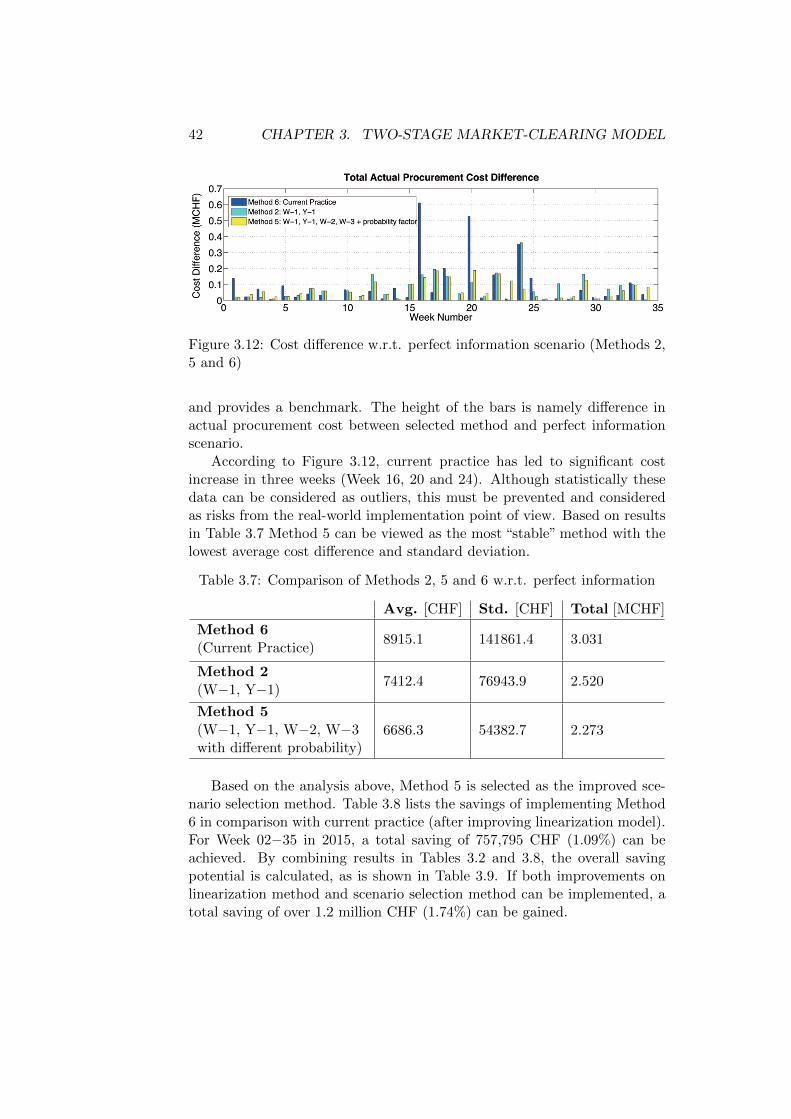
42 CHAPTER 3. TWO-STAGE MARKET-CLEARING MODEL
Figure 3.12: Cost difference w.r.t. perfect information scenario (Methods 2,5 and 6)
and provides a benchmark. The height of the bars is namely difference inactual procurement cost between selected method and perfect informationscenario.
According to Figure 3.12, current practice has led to significant costincrease in three weeks (Week 16, 20 and 24). Although statistically thesedata can be considered as outliers, this must be prevented and consideredas risks from the real-world implementation point of view. Based on resultsin Table 3.7 Method 5 can be viewed as the most “stable” method with thelowest average cost difference and standard deviation.
Table 3.7: Comparison of Methods 2, 5 and 6 w.r.t. perfect information
Avg. [CHF] Std. [CHF] Total [MCHF]
Method 6(Current Practice)
8915.1 141861.4 3.031
Method 2(W−1, Y−1)
7412.4 76943.9 2.520
Method 5(W−1, Y−1, W−2, W−3with different probability)
6686.3 54382.7 2.273
Based on the analysis above, Method 5 is selected as the improved sce-nario selection method. Table 3.8 lists the savings of implementing Method6 in comparison with current practice (after improving linearization model).For Week 02−35 in 2015, a total saving of 757,795 CHF (1.09%) can beachieved. By combining results in Tables 3.2 and 3.8, the overall savingpotential is calculated, as is shown in Table 3.9. If both improvements onlinearization method and scenario selection method can be implemented, atotal saving of over 1.2 million CHF (1.74%) can be gained.

3.3. IMPROVEMENTS OF TWO-STAGE MODEL 43
Table 3.8: Estimation of savings by improved scenario selection method(Week 02−35, 2015)
Total Savings in CHF 757,795
Total Savings in % 1.09
Average Savings per Week in CHF 22,288
Table 3.9: Estimation of savings by implementing both improvements (Week02−35, 2015)
Total Savings in CHF 1,213,167
Total Savings in % 1.74
Average Savings per Week in CHF 35,681

44 CHAPTER 3. TWO-STAGE MARKET-CLEARING MODEL

Chapter 4
Three-Stage Market-ClearingModel
In this chapter, a three-stage stochastic market-clearing market is proposed.Firstly, motivation and decision making process are introduced in Section4.1. Section 4.2 mainly focuses on the formulation of the three-stage model.In Section 4.3, how third-stage scenarios are generated and selected is illus-trated. Simulation results are demonstrated in Section 4.4.
4.1 Introduction
In Switzerland, a majority of ancillary services providers are hydro units.The available generation power of hydro power plants are very much de-pendent on seasonal pattern and weather conditions, which can be ratherunpredictable. Based on market observations, it is probable that during wa-ter peak seasons, hydro units still have unsold power in real-time operationand have to either get rid of the additional power at a very low price or topay a penalty for power imbalances it incurs. Furthermore, there has beena growing trend of RES units participating in ancillary services provision.These units are mainly wind or photovoltaic generators, whose power outputis highly unforeseeable and intermittent.
The current market model which clears at most once per day is notadapted for such changes. Therefore, an additional market stage where re-dundant power can be sold or bought as reserves is highly desirable, fromboth TSO’s and provider’s perspective. Providers gain more flexibility inbidding and will be exempted from power imbalance payments if tradingsucceeds. For Swissgrid, having the possibility of procuring cheaper reservescloser to real-time operation can potentially reduce the amount of moreexpensive reserves bought in weekly and daily market, thus achieving finan-cial gains in reserve procurement cost. Based on these motivations, such amarket is very likely to appear within the framework of the Swiss ancillary
45

46 CHAPTER 4. THREE-STAGE MARKET-CLEARING MODEL
services market.
In this thesis, we assume that there will be a new market stage: hourlymarket. This hourly market will be cleared every hour after the trading inspot market closes. With this assumption, a three-stage stochastic market-clearing model needs to be developed, which is exactly the main purpose ofthis thesis.
The decision-making process of the three-stage market can be illustratedby Figure 4.1. At the first stage when the weekly market is cleared, only bidsin weekly market are known. The rest of the bids (daily market and hourlymarket) are yet uncertain and are therefore represented by scenarios. Aftermarket-clearing, results pertaining to the acceptance of weekly bids as well assuggested procurement volume in the daily and hourly market are obtained.Weekly decisions are then given to the clearing of daily market as input. Atthis second stage, the daily market is to be cleared with available daily bidsand still unknown hourly bids, which are again modelled as scenarios (canbe different from those used in the first stage as more information couldbe collected). At the final stage, the hourly market will be cleared withdecisions from the previous two stages as well as actual bids in the hourlymarket.
Since this three-stage reserve market is still conceptual in Switzerland,no concrete market data are available to help construct hourly scenarios, letalone the update and realization of hourly bids. Therefore, this thesis willonly focus on the weekly clearing model, which is the three-stage stochasticmarket-clearing model.
Figure 4.1: Three-stage stochastic market-clearing scheme

4.2. STOCHASTIC MARKET-CLEARING MODEL 47
4.2 Stochastic Market-Clearing Model
This section will step by step unveil the three-stage stochastic market-clearing model. Decision variables and objective function are explained inSections 4.2.1 and 4.2.2. Section 4.2.3 is dedicated to the non-anticipativityconsidered in this three-stage problem. Section 4.2.4 adapts dimensioningcriteria to the three-stage model and updates the constraints. The completeformulation of the model is presented in Section 4.2.5.
4.2.1 Decision Variables
Intuitively, decision variables in the three-stage model can be grouped intofirst-stage decision variables, second-stage decision variables and third-stagedecision variables. The definition and notation of first- and second-stagedecision variables are exactly identical with those in the two-stage model,as introduced in Section 3.2.1.
For the third stage, a set of scenarios are created to represent uncer-tainty in the hourly market. Here, we assume that there does not exist anycorrelation between daily and hourly scenarios. Therefore, scenarios used inthird stage can be formulated as a combination of scenarios for daily andhourly market:
(ωd, ωh
). Each scenario combination is associated with a set
of third-stage decision variables: xh(ωd, ωh):
xh(ωd, ωh) = [xhT+
(ωd, ωh),xhT−(ωd, ωh)], (4.1)
where
• ωh ∈ Ωh is the index of scenarios for hourly market
• Ωh contains NhΩ scenarios for hourly market
• xhT+
(ωd, ωh
)∈ R168×1 is the amount of TCR+ to be procured in the
hourly market in each hour for scenario combination(ωd, ωh
)• xh
T−
(ωd, ωh
)∈ R168×1 is the amount of TCR− to be procured in the
hourly market in each hour for scenario combination(ωd, ωh
)In the third stage, TCR market is cleared for each individual hour. Since
the three-stage market-clearing model is valid for one week (24 × 7 = 168hours), length of third-stage parameters and variables is often 168.
4.2.2 Objective Function
Similar to the two-stage model, the objective function in the three-stagemarket-clearing model can be split into three terms, each representing onestage. The terms of previous two stages are exactly the same as in Section
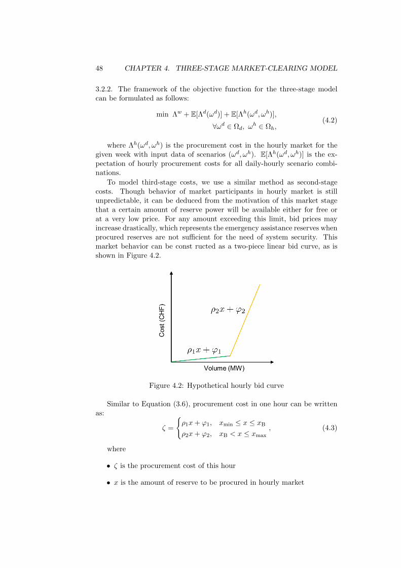
48 CHAPTER 4. THREE-STAGE MARKET-CLEARING MODEL
3.2.2. The framework of the objective function for the three-stage modelcan be formulated as follows:
min Λw + E[Λd(ωd)] + E[Λh(ωd, ωh)],
∀ωd ∈ Ωd, ωh ∈ Ωh,
(4.2)
where Λh(ωd, ωh) is the procurement cost in the hourly market for thegiven week with input data of scenarios (ωd, ωh). E[Λh(ωd, ωh)] is the ex-pectation of hourly procurement costs for all daily-hourly scenario combi-nations.
To model third-stage costs, we use a similar method as second-stagecosts. Though behavior of market participants in hourly market is stillunpredictable, it can be deduced from the motivation of this market stagethat a certain amount of reserve power will be available either for free orat a very low price. For any amount exceeding this limit, bid prices mayincrease drastically, which represents the emergency assistance reserves whenprocured reserves are not sufficient for the need of system security. Thismarket behavior can be const ructed as a two-piece linear bid curve, as isshown in Figure 4.2.
Figure 4.2: Hypothetical hourly bid curve
Similar to Equation (3.6), procurement cost in one hour can be writtenas:
ζ =
ρ1x+ ϕ1, xmin ≤ x ≤ xB
ρ2x+ ϕ2, xB < x ≤ xmax
, (4.3)
where
• ζ is the procurement cost of this hour
• x is the amount of reserve to be procured in hourly market
4.2. STOCHASTIC MARKET-CLEARING MODEL 49
• (ρ1, ϕ1) and (ρ2, ϕ2) are fitting parameters of the first and secondpart of the hourly bid curve respectively
• xmin and xmax are lower and upper bound of the bid curve
• xB is the breaking point of the linearized bid curve
Provided that ρ2 > ρ1, Equation (4.3) can be reformulated as a opti-mization problem:
minx
ζ
s.t. ρ1x+ ϕ1 ≤ ζ,ρ2x+ ϕ2 ≤ ζ,
xmin ≤ x ≤ xmax.
(4.4)
Extending the single-hour optimization to 168 hours within a week andconsidering all scenario combinations, the full version of Equation (4.4) ispresented in Equation (4.5).
minxhT+
(ωd,ωh), xhT−
(ωd,ωh)ζT+(ωd, ωh) + ζT−(ωd, ωh),
s.t. ρ+1 (ωh)xh
T+(ωd, ωh) +ϕ+
1 (ωh) ≤ ζT+(ωd, ωh),
ρ+2 (ωh)xh
T+(ωd, ωh) +ϕ+
2 (ωh) ≤ ζT+(ωd, ωh),
ρ−1 (ωh)xhT−
(ωd, ωh) +ϕ−1 (ωh) ≤ ζT−(ωd, ωh),
ρ−2 (ωh)xhT−
(ωd, ωh) +ϕ−2 (ωh) ≤ ζT−(ωd, ωh),
xhT+
(ωd, ωh) ∈ [xminh,T+
(ωh), xmaxh,T+
(ωh)],
xhT−
(ωd, ωh) ∈ [xminh,T−
(ωh), xmaxh,T−
(ωh)],
∀ωd ∈ Ωd, ∀ωh ∈ Ωh,(4.5)
where
• ζT+(ωd, ωh) ∈ R168×1 is the hourly cost vector of TCR+
• ζT−(ωd, ωh) ∈ R168×1 is the hourly cost vector of TCR−
• ρ+1 (ωh),ϕ+
1 (ωh),ρ+2 (ωh),ϕ+
2 (ωh) ∈ R168×1 are linear coefficients ofTCR+ hourly bid curves and are only dependent on hourly scenarioωh
• ρ−1 (ωh),ϕ−1 (ωh),ρ−2 (ωh),ϕ−2 (ωh) ∈ R168×1 are linear coefficients ofTCR− hourly bid curves and are only dependent on hourly scenarioωh
• xminh,T+
(ωh), xmaxh,T+
(ωh) are lower and upper bound of TCR+ bid curve
• xminh,T−
(ωh), xmaxh,T−
(ωh) are lower and upper bound of TCR− bid curve
50 CHAPTER 4. THREE-STAGE MARKET-CLEARING MODEL
Therefore, the term E[Λh(ωd, ωh)] in Equation (4.2) can be reformulatedas:
E[Λh(ωd, ωh)] =∑
ωd∈Ωd,ωh∈Ωh
πd
(ωd)πh
(ωh) [
11×168ζT+(ωd, ωh) + 11×168ζT−(ωd, ωh)],
(4.6)where πh
(ωh)
is the probability of hourly scenario ωh.
4.2.3 Non-anticipativity Matrix
Non-anticipativity can be explained as the link between different stages.This is particularly important in multi-stage problems. The principle ofnon-anticipativity is: “if realizations of stochastic processes are identical upto stage k, the values of decision variables must be identical up to stagek” [11].
In our problem, although daily scenarios and hourly scenarios are consid-ered as “decoupled”, it is still important to link third-stage decision variableswith the corresponding second-stage decision variables. This link is estab-lished through a non-anticipativity matrix An. The number of rows corre-sponds to the product of 168 (hours in a week), the number of daily scenariosNd
Ω, and the number of hourly scenarios NhΩ. The number of columns is the
product of 42 (time blocks in a week) and the number of daily scenarios NdΩ.
The value of a single element in the non-anticipativity maxtrixAn(ij,mn)is 1, if:
1. hour i is included in time block m, and
2. scenario combination j is identical with scenario n at second stage
where
• i is the index of the corresponding hour
• j is the index of the corresponding scenario combination
• m is the index of the corresponding time block
• n is the index of the corresponding scenario in second stage
Illustrative Example: Assume that there are 2 scenarios for daily market:ωd
1 , ωd2 , and 2 scenarios for hourly market: ωh
1 , ωh2 . Hence, there are in total
4 scenario combinations:
(ωd1 , ω
h1 ), (ωd
1 , ωh2 ), (ωd
2 , ωh1 ), (ωd
2 , ωh2 ) (4.7)
Consider 2 time blocks with 4 hours each:
p1 = (t1, t2, t3, t4), p2 = (t5, t6, t7, t8) (4.8)

4.2. STOCHASTIC MARKET-CLEARING MODEL 51
Decision variable vector for second stage is:
xd =[x
(1)d , x
(2)d , x
(3)d , x
(4)d
]=[xdp1(ωd
1), xdp2(ωd1), xdp1(ωd
2), xdp2(ωd2)].
(4.9)
Decision variable vector for third stage is:
xh =[xht1(ωd
1 , ωh1 ), xht2(ωd
1 , ωh1 ), xht3(ωd
1 , ωh1 ), xht4(ωd
1 , ωh1 ),
xht5(ωd1 , ω
h1 ), xht6(ωd
1 , ωh1 ), xht7(ωd
1 , ωh1 ), xht8(ωd
1 , ωh1 )
xht1(ωd1 , ω
h2 ), xht2(ωd
1 , ωh2 ), xht3(ωd
1 , ωh2 ), xht4(ωd
1 , ωh2 ),
xht5(ωd1 , ω
h2 ), xht6(ωd
1 , ωh2 ), xht7(ωd
1 , ωh2 ), xht8(ωd
1 , ωh2 ),
xht1(ωd2 , ω
h1 ), xht2(ωd
2 , ωh1 ), xht3(ωd
2 , ωh1 ), xht4(ωd
2 , ωh1 ),
xht5(ωd2 , ω
h1 ), xht6(ωd
2 , ωh1 ), xht7(ωd
2 , ωh1 ), xht8(ωd
2 , ωh1 ),
xht1(ωd2 , ω
h2 ), xht2(ωd
2 , ωh2 ), xht3(ωd
2 , ωh2 ), xht4(ωd
2 , ωh2 ),
xht5(ωd2 , ω
h2 ), xht6(ωd
2 , ωh2 ), xht7(ωd
2 , ωh2 ), xht8(ωd
2 , ωh2 )].
(4.10)
The first four variables in Equation (4.10) correspond to second-stagescenario ωd
1 and time block 1, and are thus linked to second-stage decision
variable x(1)d . The next four variables in Equation (4.10) are related to
second-stage scenario ωd1 and time block 2, and are thus linked to second-
stage decision variable x(2)d , and so on.

52 CHAPTER 4. THREE-STAGE MARKET-CLEARING MODEL
Therefore, the non-anticipativity matrix in this case is:
1 0 0 01 0 0 01 0 0 01 0 0 00 1 0 00 1 0 00 1 0 00 1 0 01 0 0 01 0 0 01 0 0 01 0 0 00 1 0 00 1 0 00 1 0 00 1 0 00 0 1 00 0 1 00 0 1 00 0 1 00 0 0 10 0 0 10 0 0 10 0 0 10 0 1 00 0 1 00 0 1 00 0 1 00 0 0 10 0 0 10 0 0 10 0 0 1
4.2.4 Constraints
The binding factors in the three-stage market-clearing model are identicalwith those in two-stage model, as explained in Section 3.2.3. The constraintfor conditional bids in the first stage has exactly the same formulation asEquation (3.11).
4.2. STOCHASTIC MARKET-CLEARING MODEL 53
Probabilistic Dimensioning Criterion
The probabilistic criterion remains the same as Equation (3.15). However,the amount of overall reserve differs, as the additional amount of reserveprocured in hourly market should be taken into account:
Rs+ = Rs− = pᵀSxwS ,
Ro+ = pᵀSxwS + pᵀT+
xwT+
+AnxdT+
(ωd) + xhT+
(ωd, ωh),
Ro− = pᵀSxwS + pᵀT−
xwT−
+AnxdT−
(ωd) + xhT−
(ωd, ωh),
∀ωd ∈ Ωd, ∀ωh ∈ Ωh.
(4.11)
Inserting Equation (4.11) into Equation (3.15), we get:
Fs+(pᵀSxwS ) + Fs−(pᵀSx
wS )
+Fo+
(pᵀSx
wS + pᵀT+
xwT+
+AnxdT+
(ωd) + xhT+
(ωd, ωh))
+Fo−
(pᵀSx
wS + pᵀT−
xwT− +Anx
dT−(ωd) + xh
T−(ωd, ωh))≤ 0.002,
∀ωd ∈ Ωd, ∀ωh ∈ Ωh.
(4.12)
Linearization of deficit curves remains the same as in Equation (3.22).Rs+ , Rs− , Ro+ and Ro− will be replaced by Equation (4.11).
Deterministic Dimensioning Criterion
Considering reserves procured in the hourly market, Equation (3.23) can bemodified as follows:
400 ≤ pᵀT+xwT+
+AnxdT+
(ωd) + xhT+
(ωd, ωh),
∀ωd ∈ Ωd, ∀ωh ∈ Ωh.(4.13)
4.2.5 Formulation
The complete mathematical formulation of the three-stage stochastic market-clearing model is presented as follows:
54 CHAPTER 4. THREE-STAGE MARKET-CLEARING MODEL
minxw, λT+
(ωd),
λT− (ωd),
ζT+ (ωd,ωh),
ζT− (ωd,ωh)
cᵀwxw +∑
ωd∈Ωd
πd(ωd) [
11×42λT+(ωd) + 11×42λT−(ωd)]
+∑
ωd∈Ωd,ωh∈Ωh
πd(ωd)πh(ωh) [
11×168ζT+(ωd, ωh) + 11×168ζT−(ωd, ωh)]
(4.14)
s.t. Acxw ≤ bc, (4.15)
α+1 (ωd)xd
T+(ωd) + β+
1 (ωd) ≤ λT+(ωd), ∀ωd ∈ Ωd, (4.16)
α+2 (ωd)xd
T+(ωd) + β+
2 (ωd) ≤ λT+(ωd), ∀ωd ∈ Ωd, (4.17)
α+3 (ωd)xd
T+(ωd) + β+
3 (ωd) ≤ λT+(ωd), ∀ωd ∈ Ωd, (4.18)
α−1 (ωd)xdT−(ωd) + β−1 (ωd) ≤ λT−(ωd), ∀ωd ∈ Ωd, (4.19)
α−2 (ωd)xdT−(ωd) + β−2 (ωd) ≤ λT−(ωd), ∀ωd ∈ Ωd, (4.20)
α−3 (ωd)xdT−(ωd) + β−3 (ωd) ≤ λT−(ωd), ∀ωd ∈ Ωd, (4.21)
ρ+1 (ωh)xh
T+(ωd, ωh) +ϕ+
1 (ωh) ≤ ζT+(ωd, ωh),
∀ωd ∈ Ωd, ∀ωh ∈ Ωh, (4.22)
ρ+2 (ωh)xh
T+(ωd, ωh) +ϕ+
2 (ωh) ≤ ζT+(ωd, ωh),
∀ωd ∈ Ωd, ∀ωh ∈ Ωh, (4.23)
ρ−1 (ωh)xhT−(ωd, ωh) +ϕ−1 (ωh) ≤ ζT−(ωd, ωh),
∀ωd ∈ Ωd, ∀ωh ∈ Ωh, (4.24)
ρ−2 (ωh)xhT−(ωd, ωh) +ϕ−2 (ωh) ≤ ζT−(ωd, ωh),
∀ωd ∈ Ωd, ∀ωh ∈ Ωh, (4.25)
a(i)s+
(pᵀSx
wS
)+ b(i)s+ ≤ εs+ , i = 1, · · · ,m, (4.26)
a(i)s−
(pᵀSx
wS
)+ b(i)s− ≤ εs− , i = 1, · · · , n, (4.27)
a(i)o+
(pᵀSx
wS + pᵀT+
xwT+
+AnxdT+
(ωd) + xhT+
(ωd, ωh))
+ b(i)o+ ≤ εo+ ,
∀ωd ∈ Ωd, i = 1, · · · , j, (4.28)
a(i)o−
(pᵀSx
wS + pᵀT−
xwT− +Anx
dT−(ωd) + xh
T−(ωd, ωh))
+ b(i)o− ≤ εo− ,
∀ωd ∈ Ωd, i = 1, · · · , k, (4.29)
εs+ + εs− + εo+ + εo− ≤ 0.002, (4.30)
400 ≤ pᵀT+xwT+
+AnxdT+
(ωd) + xhT+
(ωd, ωh), ∀ωd ∈ Ωd, (4.31)
xdT+
(ωd) ∈ [xmind,T+
(ωd), xmaxd,T+
(ωd)], ∀ωd ∈ Ωd, (4.32)
xdT−(ωd) ∈ [xmin
d,T−(ωd), xmaxd,T−(ωd)], ∀ωd ∈ Ωd, (4.33)
xhT+
(ωd, ωh) ∈ [xminh,T+
(ωh), xmaxh,T+
(ωh)], ∀ωd ∈ Ωd, ∀ωh ∈ Ωh,
(4.34)
xhT−(ωd, ωh) ∈ [xmin
h,T−(ωh), xmaxh,T−(ωh)], ∀ωd ∈ Ωd, ∀ωh ∈ Ωh.
(4.35)
4.3. SCENARIOS FOR HOURLY MARKET 55
Constraint (4.15) corresponds to the conditional bids received in theweekly market. Constraints (4.16)−(4.21) are related to three-piece dailycost curve. Constraints (4.22)−(4.25) are related to hourly cost curve.(4.26)−(4.30) are associated with probabilistic dimensioning criterion. Con-straint (4.31) is for deterministic dimensioning criterion (MEAS constraint).Constraints (4.32) and (4.33) define feasible ranges for daily procurementamounts, whereas constraints (4.34) and (4.34) define feasible ranges forhourly procurement amounts.
4.3 Scenarios for Hourly Market
4.3.1 Modelling of Hourly Bid Curves
As is mentioned previously, the hourly market has not yet been establishedin Switzerland and no market data are available, which is the biggest chal-lenge in building scenarios for hourly market. Figure 4.2 presented how ahypothetical hourly bid curve is constructed. Key parameters are slopes ofboth pieces and the breaking point.
Breaking Point
In the current market setting, providers with additional available power maysubmit bids into TCE market, which will be referred to as free TCE bidshereafter. These bids are not bound with a previously accepted reserve bidand can represent real-time available capacity of power plants to a certainextent. Nevertheless, since not many BGs are submitting such bids, estima-tions based on these data may turn out to be conservative.
Making use of these free TCE bids does not require any procurement ofthe corresponding reserve volume, which can save reserve costs. Therefore,the total volume of free TCE bids can be in a way regarded as the breakingpoint of the bid curve presented in Figure 4.2. Prior to this breaking point,the curve has a very small slope, which corresponds to the cheap or evenfree reserves that can be procured in the hourly market.
Slope
Although breaking point is the key binding parameter in the hourly bidcurve, it is still important to select adequate slopes for the first and secondlinear pieces.
The slope of the first piece has to be very low in order to reflect thenature of these capacity. However, it cannot be set to 0, since it wouldresult in multiple solutions of the optimization problem.
The slope of the second piece needs to be relatively large, as it representsthe cost of emergency reserves in case the procured reserves are not sufficient.

56 CHAPTER 4. THREE-STAGE MARKET-CLEARING MODEL
This price has to be realistic as well. Otherwise, the solution will alwaysbe driven to the first piece, which undermines the motivation of having thesecond piece.
Based on the criteria above and sensitivity analysis, the slope of thefirst piece is defined as 0.1 CHF/MW, while the slope of the second piece ischosen to be 200 CHF/MW.
4.3.2 Scenario Construction
Since slopes of hourly bid curve are assumed to be constants, key parameterin hourly scenarios is the breaking point, or the volume of free TCE bids.
010
2030
40 Mon Tue Wed Thu Fri Sat Sun
0
100
200
300
Free TCE+ Capacity
Week Number
MW
0
50
100
150
200
250
Figure 4.3: Free TCE+ volume in 2015 (Week 01−35)
010
2030
40MonTueWedThuFriSatSun
0
100
200
300
Free TCE− Capacity
Week Number
MW
0
50
100
150
200
Figure 4.4: Free TCE− volume in 2015 (Week 01−35)
Figures 4.3 and 4.4 illustrate the free TCE volume in the current market.It is noticeable that both positive and negative products are subject to a
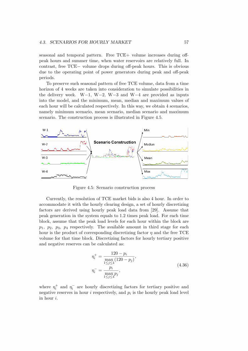
4.3. SCENARIOS FOR HOURLY MARKET 57
seasonal and temporal pattern. Free TCE+ volume increases during off-peak hours and summer time, when water reservoirs are relatively full. Incontrast, free TCE− volume drops during off-peak hours. This is obviousdue to the operating point of power generators during peak and off-peakperiods.
To preserve such seasonal pattern of free TCE volume, data from a timehorizon of 4 weeks are taken into consideration to simulate possibilities inthe delivery week. W−1, W−2, W−3 and W−4 are provided as inputsinto the model, and the minimum, mean, median and maximum values ofeach hour will be calculated respectively. In this way, we obtain 4 scenarios,namely minimum scenario, mean scenario, median scenario and maximumscenario. The construction process is illustrated in Figure 4.5.
Figure 4.5: Scenario construction process
Currently, the resolution of TCE market bids is also 4 hour. In order toaccommodate it with the hourly clearing design, a set of hourly discretizingfactors are derived using hourly peak load data from [29]. Assume thatpeak generation in the system equals to 1.2 times peak load. For each timeblock, assume that the peak load levels for each hour within the block arep1, p2, p3, p4 respectively. The available amount in third stage for eachhour is the product of corresponding discretizing factor η and the free TCEvolume for that time block. Discretizing factors for hourly tertiary positiveand negative reserves can be calculated as:
η+i =
120− pimax
1≤j≤4(120− pj)
,
η−i =pi
max1≤j≤4
pj,
(4.36)
where η+i and η−i are hourly discretizing factors for tertiary positive and
negative reserves in hour i respectively, and pi is the hourly peak load levelin hour i.

58 CHAPTER 4. THREE-STAGE MARKET-CLEARING MODEL
The calculated hourly discretizing factors are shown in Appendix A.As hourly market has not yet been established, scenarios selected above
represent different possible levels of available bid volume in this new market.In a full set of scenarios for hourly market, all four scenarios are incorporatedand assigned with different probability factors, which are shown in Table 4.1.These probabilities are selected based on sensitivity analysis.
Table 4.1: Probability factors of hourly scenarios
Scenario Probability
Minimum 5%
Median 45%
Mean 45%
Maximum 5%
4.4 Simulation Results
This section presents simulation results of the proposed three-stage stochas-tic market-clearing model. Section 4.4.1 studies the impact of adding athird stage by investigating different hourly scenarios . In Section 4.4.2, afull set of daily and hourly scenarios will be considered and results will bedemonstrated.
4.4.1 Case Study: Impact of Hourly Market
The objective of this case study is to investigate the influence of hourlymarket scenarios on optimization results. Therefore, six cases are simulatedand compared. For convenience, perfect information scenario is selectedfor second stage. These six cases only differ in the selection of third-stagescenarios and are defined in Figure 4.6.
• Case “Two-Stage” refers to the two-stage model with perfect informa-tion as second-stage scenario, which is a deterministic market-clearing.
• Cases “Min”, “Median”, “Mean” and “Max” are deterministic three-stage market-clearing models where minimum, median, mean and max-imum scenarios are inputs for third-stage scenario respectively.
• Case “Full” refers to the case where a full set of hourly scenarios (min-imum, median, mean, maximum) are imported and assigned with dif-ferent probability factors.
The 6 cases are simulated on 8 selected weeks in 2015. Informationregarding these 8 weeks can be found in Table 3.6. Results in terms ofreserve procurement and total cost of procurement are presented as follows.

4.4. SIMULATION RESULTS 59
Figure 4.6: Definition of cases
Reserve Amount
For each selected week, six optimization models are run and decisions areobtained regarding accepted bids in weekly market and suggested procure-ment volume in daily and hourly market. Since decisions regarding daily andhourly market are associated with each hour/time block and each scenario,an average procurement volume is calculated. Two typical weeks (Week04 and Week 35) are selected here to illustrate the impact of third stagescenarios on procurement decisions.
Figure 4.7 shows the amount of SCR and TCR procured in each market.As can be seen from the figure, as the available volume in hourly marketincreases (from “Two-Stage” to “Max”), the volume of reserves procured inhourly market increases correspondingly. This is due to the fact that hourlyreserves are generally more attrative in terms of pricing. As a consequence,the amount of reserves procured in daily market reduces, which can be re-garded as the substitution effect between daily and hourly products. Theamount of SCR and overall reserves, however, remains constant, as it is theoptimum to satisfy dimensioning criteria.
In Figure 4.8, we can observe that the total amount of reserves changesaccording to different cases. A slight difference in the procured amountof SCR explains this phenomenon. As SCR is generally more expensive(3-5 times) than TCR, it is possible that more TCR is procured in orderto compensate for SCR, which leads to lower procurement cost. This canbe considered as an outcome of dimensioning reserves using probabilisticcriterion in Equation (3.15).
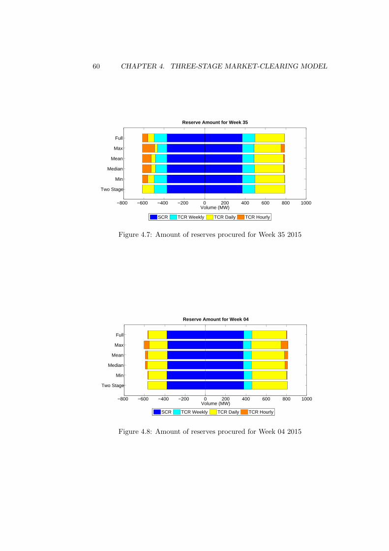
60 CHAPTER 4. THREE-STAGE MARKET-CLEARING MODEL
−800 −600 −400 −200 0 200 400 600 800 1000
Two Stage
Min
Median
Mean
Max
Full
Volume (MW)
Reserve Amount for Week 35
SCR TCR Weekly TCR Daily TCR Hourly
Figure 4.7: Amount of reserves procured for Week 35 2015
−800 −600 −400 −200 0 200 400 600 800 1000
Two Stage
Min
Median
Mean
Max
Full
Volume (MW)
Reserve Amount for Week 04
SCR TCR Weekly TCR Daily TCR Hourly
Figure 4.8: Amount of reserves procured for Week 04 2015

4.4. SIMULATION RESULTS 61
Total Cost of Procurement
Total procurement cost is calculated as the sum of weekly, daily and hourlyreserve costs. For full scenario case, the hourly cost is the expected cost ofall hourly scenarios. The total procurement cost of each three-stage caseis benchmarked with the two-stage case. Cost savings in percentage areobtained and presented in Table 4.2 and Figure 4.9.
From the results we can see that incorporating an hourly market canachieve an average saving of up to 3.11% in the maximum case. This canbe an indicator for future market design, as it reveals the potential of hav-ing an hourly market. If the liquidity of third-stage market is similar tothe free TCE volume nowadays, “mean” and “median” cases can representfuture market situation, in which around 1.5% can be saved. To be moreconservative, the minimum case is considered, which still provides 0.35%savings. The “full” scenarios case is somewhat close to minimum case, butwith slightly higher savings potential. Therefore, we can conclude that the“full scenarios” case is a rather conservative estimation of the third-stagemarket.
Table 4.2: Potential cost savings w.r.t. two-stage model
Min Median Mean Max Full
Week 04 0.09% 0.86% 1.06% 2.33% 0.15%
Week 08 0.31% 1.31% 1.63% 3.25% 0.38%
Week 13 0.31% 1.01% 1.49% 3.35% 0.36%
Week 17 0.03% 0.92% 1.36% 3.04% 0.19%
Week 22 0.11% 0.61% 1.14% 1.89% 0.27%
Week 26 0.48% 1.33% 1.80% 4.09% 0.49%
Week 30 0.38% 1.00% 1.20% 2.24% 0.41%
Week 35 1.10% 2.26% 2.72% 4.66% 1.16%
Average 0.35% 1.16% 1.55% 3.11% 0.43%
4.4.2 Complete Scenario Simulations
In this section, simulation results with a complete set of second-stage andthird-stage scenarios are presented. Method 5 in Figure 3.10 is selected assecond-stage scenarios. All four hourly scenarios (min, median, mean, max)are incorporated into third stage with probabilities given in Table 4.1. Intotal, 16 scenario combinations are considered. The whole scenario tree ispresented in Figure 4.10. Notations of scenarios are defined in Table 4.3.
The size of the optimization problem is shown in Table 4.4. For Week 042015, there are in total 17,090 decision variables and 108,905 constraints (theexact number may vary according to number of weekly bids). The problemis solved with CPLEX using a commercial package TOMLAB in Matlab.
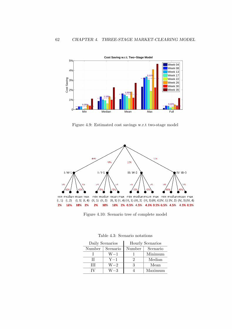
62 CHAPTER 4. THREE-STAGE MARKET-CLEARING MODEL
Min Median Mean Max Full0
1%
2%
3%
4%
5%
Cos
t Sav
ing
Cost Saving w.r.t. Two−Stage Model
Week 04Week 08Week 13Week 17Week 22Week 26Week 30Week 35
3.11%
1.16%
1.55%
0.43%0.35%
Figure 4.9: Estimated cost savings w.r.t two-stage model
Figure 4.10: Scenario tree of complete model
Table 4.3: Scenario notations
Daily Scenarios Hourly Scenarios
Number Scenario Number Scenario
I W−1 1 Minimum
II Y−1 2 Median
III W−2 3 Mean
IV W−3 4 Maximum

4.4. SIMULATION RESULTS 63
The average computation time is around 20-25 minutes on ordinary per-sonal computers, which is satisfying for three-stage stochastic programmingproblems and affordable for real market clearing.
Table 4.4: Problem size
First-Stage Variables288(Depending on number of bids)
Second-Stage Variables 42× 4× 2 + 42× 4× 2 = 672
Third-Stage Variables 168×16×2 + 168×16×2 = 10, 752
Variables for Deficit Rate 2 + 168× 16× 2 = 5, 378
Constraints for Conditional Bids22(Depending on number of bids)
Constraints for MEAS 168× 16 = 2, 688
Constraints for Deficit Curve88, 722(Depending on number of pieces)
Constraints for Daily Cost 1, 344
Constraints for Hourly Cost 10, 752
Constraints for Reserve Amount 5, 377
Reserve Amount
Figure 4.11 and Table 4.5 show simulated reserve procurement amount forthe 8 selected weeks. Daily and hourly reserve amount is calculated as themean value of different scenarios and hour/time blocks. We can get thefollowing takeaways from these results:
1. During summer (July and August), more reserve is available in thehourly market. This leads to less procurement in the daily market,and even reduces the amount of SCR procured in the weekly market.However, a growing share of hourly TCR+ is not witnessed in Week30 and 35. This is partially due to the unusual hot summer in Europein 2015. Most Swiss producers exported their produced electricity toItaly, where demand is extraordinarily high due to air conditioning.
2. During winter and spring seasons, a scarcity of water is expected.Thus, not much available power in the hourly market is anticipated.As a result, more weekly and daily products are procured in order toguarantee system security.
3. Comparing Week 22 and 30, we can roughly estimate that 1 MW ofTCR− can compensate for 2 MW of TCR+. The comparison be-tween Week 26 and 30 shows that 1 MW SCR can be replaced byapproximately 11 MW TCR−. These relationships provide basis for

64 CHAPTER 4. THREE-STAGE MARKET-CLEARING MODEL
substitutions between different products while obeying system securitycriteria.
−800 −600 −400 −200 0 200 400 600 800 1000
Week 04
Week 08
Week 13
Week 17
Week 22
Week 26
Week 30
Week 35
Reserve Amount with Complete Scenarios
Volume (MW)
SCR
TCR Weekly
TCR Daily
TCR Hourly
Figure 4.11: Reserve amount of complete model
Table 4.5: Amount of reserves procured in complete model
SCR [MW] TCR+ [MW] TCR− [MW]
Week 04 385 415 159
Week 08 375 428 219
Week 13 371 451 248
Week 17 380 408 190
Week 22 370 413 271
Week 26 375 403 221
Week 30 370 405 275
Week 35 372 424 241
Total Cost of Procurement
The total expected cost of procurement is calculated for each week and thencompared with that of the two-stage model with identical daily scenarios.Results are presented in Table 4.6.
Table 4.6 conveys the message that on average 10,767 CHF can be savedby using a three-stage market-clearing. This result is based on the hypothesisthat all improvements suggested in Section 3.3 are implemented on the two-stage model. If we count in savings brought by these improvements, morefinancial benefits could be gained.
Moreover, these results are based on the conservative third-stage selec-tion method (which considers minimum scenario). In the future when thethird-stage market is established, it is highly probable that Swissgrid will
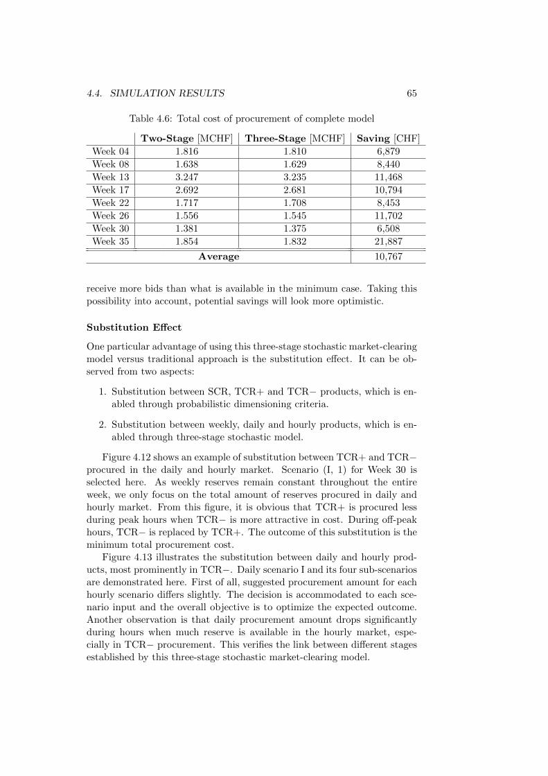
4.4. SIMULATION RESULTS 65
Table 4.6: Total cost of procurement of complete model
Two-Stage [MCHF] Three-Stage [MCHF] Saving [CHF]
Week 04 1.816 1.810 6,879
Week 08 1.638 1.629 8,440
Week 13 3.247 3.235 11,468
Week 17 2.692 2.681 10,794
Week 22 1.717 1.708 8,453
Week 26 1.556 1.545 11,702
Week 30 1.381 1.375 6,508
Week 35 1.854 1.832 21,887
Average 10,767
receive more bids than what is available in the minimum case. Taking thispossibility into account, potential savings will look more optimistic.
Substitution Effect
One particular advantage of using this three-stage stochastic market-clearingmodel versus traditional approach is the substitution effect. It can be ob-served from two aspects:
1. Substitution between SCR, TCR+ and TCR− products, which is en-abled through probabilistic dimensioning criteria.
2. Substitution between weekly, daily and hourly products, which is en-abled through three-stage stochastic model.
Figure 4.12 shows an example of substitution between TCR+ and TCR−procured in the daily and hourly market. Scenario (I, 1) for Week 30 isselected here. As weekly reserves remain constant throughout the entireweek, we only focus on the total amount of reserves procured in daily andhourly market. From this figure, it is obvious that TCR+ is procured lessduring peak hours when TCR− is more attractive in cost. During off-peakhours, TCR− is replaced by TCR+. The outcome of this substitution is theminimum total procurement cost.
Figure 4.13 illustrates the substitution between daily and hourly prod-ucts, most prominently in TCR−. Daily scenario I and its four sub-scenariosare demonstrated here. First of all, suggested procurement amount for eachhourly scenario differs slightly. The decision is accommodated to each sce-nario input and the overall objective is to optimize the expected outcome.Another observation is that daily procurement amount drops significantlyduring hours when much reserve is available in the hourly market, espe-cially in TCR− procurement. This verifies the link between different stagesestablished by this three-stage stochastic market-clearing model.
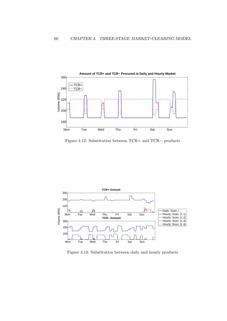
66 CHAPTER 4. THREE-STAGE MARKET-CLEARING MODEL
Mon Tue Wed Thu Fri Sat Sun
180
200
220
240
260Amount of TCR+ and TCR− Procured in Daily and Hourly Market
Vol
ume
(MW
)
TCR+TCR−
Figure 4.12: Substitution between TCR+ and TCR− products
Mon Tue Wed Thu Fri Sat Sun
100
200
300TCR+ Amount
Vol
ume
(MW
)
Mon Tue Wed Thu Fri Sat Sun
100
200
300TCR− Amount
Daily: Scen. IHourly: Scen. (I, 1)Hourly: Scen. (I, 2)Hourly: Scen. (I, 3)Hourly: Scen. (I, 4)
Figure 4.13: Substitution between daily and hourly products

Chapter 5
Conclusions and Outlook
5.1 Summary
This thesis focuses on the market-clearing model of the Swiss reserve market.The current design of the Swiss reserve market is composed of a weeklyauction and a daily auction. Secondary reserves (fast reserves that are highquality products) are procured in the weekly market, while the amount oftertiary reserves (slow reserves) is split between the weekly and daily market.On the basis of a two-stage stochastic market-clearing model which has beenimplemented since January 2014, this thesis proposes some improvementsof the current two-stage model and develops a novel three-stage stochasticmarket-clearing model to accommodate with future market design. Morespecifically, major contributions of this thesis can be summarized as follows:
1. Scenarios for daily market are investigated. Firstly, different lineariza-tion methods of daily bid curve are compared. A three-piece lineariza-tion method based on least squares estimation is chosen, which is moreaccurate than current practice and is able to reduce total cost. Then,9 scenario selection methods are experimented. Based on simulationresults, the method containing W−1, Y−1, W−2, W−3 with differentprobability factors assigned to each scenario is selected. Based on theestimation of 34 weeks in 2015, these improvements can achieve anoverall cost saving of 1.74%. The improvements can be readily imple-mented on the current two-stage market-clearing model in Switzerland.
2. The framework and the formulation of a three-stage stochastic market-clearing model are proposed. In addition to the current market stages,an hourly market is considered where reserves are available at a verylow cost or even for free. Scenarios for hourly market are constructedand selected based on analysis of free TCE bids in the current market.These data provide a reference for future market situation.
3. The proposed three-stage model is simulated with different scenario
67

68 CHAPTER 5. CONCLUSIONS AND OUTLOOK
inputs. Firstly, single scenario in hourly market is considered in orderto gain insight into the impact of third stage. Results show that in amost optimistic case, over 3% saving can be achieved by having a thirdstage. Secondly, a complete set of scenarios (including 4 daily scenariosand 4 hourly scenarios) are implemented. Reserve amount and totalprocurement cost are presented. On average the three-stage model cansave 10,767 CHF per week in comparison with the improved two-stagemodel. Lastly, substitution effects in the stochastic market-clearingmodels are illustrated with examples.
So far, the application of a three-stage stochastic market-clearing modelin the reserve market, especially from TSO perspective, is novel. The wholework of this thesis is based on real-world market data. The improvements oftwo-stage model can be directly implemented in the current market-clearingsystem. The three-stage model can be utilized as soon as the design of thethird-stage market goes live.
5.2 Future Work
The proposed framework and improvements are closely related to solvingreal-world problem faced by TSOs. However, a more realistic considerationwill be to include certain risk factors in the objective function. Risk-aversemodels can mitigate market risks caused by abnormal network conditionsand trading behavior. To develop this model, more information of market be-havior needs to be collected and analyzed, which can be rather non-trivial.

Appendix A
Hourly Discretizing Factors
According to Equation (4.36), hourly discretizing factors are obtained asfollows:
69

70 APPENDIX A. HOURLY DISCRETIZING FACTORS
Table A.1: Hourly discretizing factors
Winter Weeks Summer Weeks Spring/fall Weeks
1-8 & 44-52 18-30 9-17 & 31-43
Hour Weekday Weekend Weekday Weekend Weekday Weekend
00-01h 0.8689 0.7778 0.8750 0.8364 0.9194 0.8333
01-02h 0.9344 0.8889 0.9375 0.9091 0.9355 0.8704
02-03h 0.9836 0.9630 0.9688 0.9818 0.9677 0.9444
03-04h 1.0000 1.0000 1.0000 1.0000 1.0000 1.0000
04-05h 1.0000 1.0000 1.0000 0.9655 1.0000 1.0000
05-06h 0.9836 0.9821 0.9688 1.0000 0.9016 1.0000
06-07h 0.7541 0.9643 0.8750 1.0000 0.7869 0.9455
07-08h 0.5574 0.8929 0.6875 0.9310 0.5738 0.8364
08-09h 1.0000 1.0000 1.0000 1.0000 1.0000 1.0000
09-10h 0.9600 0.8000 0.7576 0.8718 0.8400 0.8378
10-11h 0.9600 0.7500 0.6364 0.7436 0.8000 0.7568
11-12h 1.0000 0.7250 0.6061 0.6923 0.8400 0.7027
12-13h 0.9259 0.9091 0.9130 0.9310 0.8438 0.8529
13-14h 0.9259 0.9697 0.8696 0.9655 0.8750 0.8824
14-15h 1.0000 1.0000 0.8696 1.0000 0.9375 0.8824
15-16h 0.9630 1.0000 1.0000 1.0000 1.0000 1.0000
16-17h 0.8750 1.0000 0.8571 1.0000 1.0000 1.0000
17-18h 0.8333 0.6897 0.8571 0.9286 0.9333 0.9143
18-19h 0.8333 0.7241 0.9643 0.8929 0.8000 0.8000
19-20h 1.0000 0.7931 1.0000 0.8929 0.7333 0.5714
20-21h 0.5088 0.6667 0.5833 0.5000 0.4800 0.6571
21-22h 0.6491 0.7179 0.5625 0.6750 0.6000 0.7143
22-23h 0.8246 0.8462 0.6875 0.8000 0.8000 0.8571
23-24h 1.0000 1.0000 1.0000 1.0000 1.0000 1.0000
Bibliography
[1] RTE. Electricity Demand. http://www.rte-france.com/en/
eco2mix/eco2mix-consommation-en (Date of access: November 16,2015).
[2] G. Andersson. Dynamics and Control of Electric Power Systems, 2014.Lecture Script, ETH Zurich.
[3] Swissgrid. Ancillary Services. https://www.swissgrid.ch/
swissgrid/en/home/experts/topics/ancillary_services.html
(Date of access: November 17, 2015).
[4] F. Abbaspourtorbati and M. Zima. The swiss reserve market: Stochas-tic programming in practice. IEEE Transactions on Power Systems,PP(99):1–7, 2015.
[5] Swissgrid. Basic principles of ancillary service products.https://www.swissgrid.ch/dam/swissgrid/experts/ancillary_
services/Dokumente/D151019_AS-Products_V9R1_en.pdf (Date ofaccess: November 17, 2015).
[6] Accuweather. Zurich Weather. http://www.accuweather.com/en/ch/zurich/316622/december-weather/316622 (Date of access: Decem-ber 2, 2015).
[7] D.S. Kirschen and G. Strbac. Fundamentals of Power System Eco-nomics. Wiley, 2004.
[8] N. Mankiw. Principles of Economics. Economics Series. Cengage Learn-ing, 2011.
[9] Regelleistung.net. Market Description. http://https://www.
regelleistung.net/ext/download/marktbeschreibung (Date of ac-cess: November 16, 2015).
[10] John R Birge and Francois Louveaux. Introduction to Stochastic Pro-gramming. Springer Science & Business Media, 2011.
71
72 BIBLIOGRAPHY
[11] Antonio J Conejo, Miguel Carrion, and Juan M Morales. Decisionmaking under uncertainty in electricity markets, volume 1. Springer,2010.
[12] Marida Bertocchi, Giorgio Consigli, and Michael AH Dempster.Stochastic Optimization Methods in Finance and Energy. Springer,2011.
[13] Alvaro Baillo, Mariano Ventosa, Michel Rivier, and Andres Ramos. Op-timal offering strategies for generation companies operating in electric-ity spot markets. IEEE Transactions on Power Systems, 19(2):745–753,2004.
[14] Chefi Triki, Antonio J Conejo, and Lina P Garces. Short-term tradingfor electricity producers. In Stochastic Optimization Methods in Financeand Energy, pages 181–201. Springer, 2011.
[15] Lina P Garces and Antonio J Conejo. Weekly self-scheduling, forwardcontracting, and offering strategy for a producer. IEEE Transactionson Power Systems, 25(2):657–666, 2010.
[16] A. Ahmadi-Khatir, A.J. Conejo, and R. Cherkaoui. Multi-area unitscheduling and reserve allocation under wind power uncertainty. IEEETransactions on Power Systems, 29(4):1701–1710, July 2014.
[17] J Aghaei, HA Shayanfar, and N Amjady. Joint market clearing in astochastic framework considering power system security. Applied En-ergy, 86(9):1675–1682, 2009.
[18] Swissgrid. Introduction to the Balance Group Model. https:
//www.swissgrid.ch/dam/swissgrid/experts/bgm/bg_documents/
en/balance_group_model_intro_en.pdf (Date of access: November20, 2015).
[19] ENTSO-E. Continental Europe Operation Handbook Policy 1:Load-Frequency Control and Performance. https://www.entsoe.
eu/fileadmin/user_upload/_library/publications/entsoe/
Operation_Handbook/Policy_1_final.pdf (Date of access: Novem-ber 12, 2015).
[20] ENTSO-E. Supporting Document for the Network Code onLoad-Frequency Control and Reserves. https://www.entsoe.eu/
fileadmin/user_upload/_library/resources/LCFR/130628-NC_
LFCR-Supporting_Document-Issue1.pdf (Date of access: November12, 2015).
BIBLIOGRAPHY 73
[21] ENTSO-E. Network Code on Load-Frequency Control and Reserves.https://www.entsoe.eu/fileadmin/user_upload/_library/
resources/LCFR/130628-NC_LFCR-Issue1.pdf (Date of access:November 12, 2015).
[22] A.J. Wood, B.F. Wollenberg, and G.B. Sheble. Power Generation,Operation and Control, 3rd Edition. John Wiley & Sons, 2014.
[23] P. Kundur, N.J. Balu, and M.G. Lauby. Power system stability andcontrol. EPRI power system engineering series. McGraw-Hill, 1994.
[24] ENTSO-E. ENTSO-E Launches a Tender for AssessingaFRR Products. https://www.entsoe.eu/news-events/
announcements/announcements-archive/Pages/News/
entsoe-launches-a-tender-for-assessing-aFRR-products.aspx
(Date of access: November 16, 2015).
[25] Swissgrid. Overview of ancillary services. https://www.swissgrid.
ch/dam/swissgrid/experts/ancillary_services/Dokumente/
D100412_AS-concept_V1R0_en.pdf (Date of access: November 17,2015).
[26] Regelleistung.net. Common Tendering for Primary Control Reserve.https://www.regelleistung.net/ext/static/prl;jsessionid=
8RM2WLLJRRvkk55RnyB68gyMMH2BCTrXlgrTq7VQ3GHblTnGXQ5H!
-1671615913!-308437016?lang=en (Date of access: November17, 2015).
[27] Swissgrid. SDL Ausschreibungskalender 2016. https://www.
swissgrid.ch/dam/swissgrid/experts/ancillary_services/
tenders/en/sdl_ausschreibungskalender_2016.pdf (Date ofaccess: November 20, 2015).
[28] Finn R Førsund. Hydropower economics, volume 217. Springer, 2015.
[29] RTS Task Force. The ieee reliability test system-1996. IEEE Transac-tions on Power System, 14(3):1010–1020, 1999.