modeling and estimation for the renal system benjamin j
TRANSCRIPT

Modeling and Estimation for the Renal System
Benjamin J. Czerwin
Submitted in partial fulfillment of the requirements for the degree of
Doctor of Philosophy under the Executive Committee
of the Graduate School of Arts and Sciences
COLUMBIA UNIVERSITY
2021

© 2021
Benjamin J. Czerwin
All Rights Reserved

Abstract
Modeling and Estimation for the Renal System
Benjamin J. Czerwin
Understanding how a therapy will impact the injured kidney before being administered
would be an asset to the clinical world. The work in this thesis advances the field of
mathematical modeling of the kidneys to aid in this cause. The objectives of this work are
threefold: 1) to develop and personalize a model to specific patients in different diseased states,
via parameter estimation, in order to test therapeutic trajectories, 2) to use parameter estimation
to understand the cause of different kidney diseases, differentiate between potential kidney
diseases, and facilitate targeted therapies, and 3) to push forward the understanding of kidney
physiology via physiology-based mathematical modeling techniques. To accomplish these
objectives, we have developed two models of the kidneys: 1) a broad, steady-state, closed-loop
model of the entire kidney with human physiologic parameters, and 2) a detailed, dynamic model
of the proximal tubule, an important part of kidney, with rat physiologic parameters. To readily
aid physicians, a human model would easily fit into the clinical workflow. Since there is a lack
of invasive human renal data for validation and parameter estimation, we employ a minimal
modeling approach. However, to aid in deeper understanding of renal function for future
applications, targeted therapy testing, and potentially replace invasive measures, we develop a
more detailed model. The development of such a model requires invasive data for validation and
parameter estimation, and hence we model for rodents, where such invasive data are more
readily available.

The kidneys are composed of approximately one million functional units known as
nephrons. The glomerular filtration rate (GFR) is the rate at which the kidney filters blood at the
start of the nephron. This filtration rate is highly regulated via several control mechanisms and
needs to be maintained within a small range in order to maintain a proper water and electrolyte
balance. Hence, fluctuations of GFR are indicative of overall kidney health. In developing the
human kidney model, we also sought to understand the relationship between blood pressure and
GFR since many therapies affect blood pressure and subsequently GFR. This model describes
steady-state conditions of the entire kidney, including renal autoregulation. Model validation is
performed with experimental data from healthy subjects and severely hypertensive patients. The
baseline model’s GFR simulation for normotensive and the manually tuned model’s GFR
simulation for hypertensive intensive care unit patients had low root mean squared errors
(RMSE) of 13.5 mL/min and 5 mL/min, respectively. These values are both lower than the error
of 18 mL/min in GFR estimates, reported in previous studies. It has been shown that vascular
resistance and renal autoregulation parameters are altered in severely hypertensive stages, and
hence, a sensitivity analysis is conducted to investigate how changes in these parameters affect
GFR. The results of the sensitivity analysis reinforce the fact that vascular resistance is inversely
related to GFR and show that changes to either vascular resistance or renal autoregulation cause
a significant change in sodium concentration in the descending limb of Henle. This is an
important conclusion as it quantifies the mapping between hypertension parameters and two
important kidney states, GFR and sodium urine levels.
Glomerulonephritis is one of the two major intra-renal kidney diseases, characterized as a
breakdown at the site of the glomerulus that affects GFR and subsequently other portions of the
nephron. This disease accounts for 15% of all kidney injuries and one-fourth of end-stage renal

disease patients. The human kidney model is used to estimate renal parameters of patients with
glomerulonephritis. The model is an implicit system and in developing an optimization algorithm
to use for parameter estimation, we modify in a novel way, the Levenberg-Marquardt
optimization using the implicit function theorem in order to calculate the Jacobian and Hessian
matrices needed. We further adapt the optimization algorithm to work for constrained
optimization since our parameter values must be physiologically feasible within a certain range.
The parameter estimation method we use is a three-step process: 1) manually adjusting
parameters for the hypertension comorbidity, 2) iteratively estimating parameters that vary from
person to person using no-kidney-injury (NKI) data, and 3) iteratively estimating parameters that
are affected by glomerulonephritis using labeled diseased data. Such a process generates a model
that is personalized to each given patient. This patient-specific model can then be used to
simulate and evaluate outcomes of potential therapies (e.g., vasodilators) on the model in lieu of
the patient, and observe how alterations in blood pressure or sodium level affect renal function.
Parameter estimation in the presence of glomerulonephritis is a challenging task due to the
complexity of the kidney physiology and the number of parameters to estimate. This is further
complicated by comorbidities such as hypertension, cardiac arrythmia, and valvular disease,
because they alter kidney physiology and hence, increase the number of parameters to estimate.
We chose to focus on hypertension since it is very prevalent in hospitals and intensive care units.
It was found that over all patients, average model estimates of GFR and urine output rate (UO)
were within 9.2 mL/min and 0.71 mL/min for NKI data. These results are expectedly better than
those achieved from the non-personalized model since the parameters are now specific to each
patient. The results also demonstrate our ability to non-invasively estimate GFR with less error
than the 18 mL/min currently possible. The estimations were validated by ensuring that the

estimated parameter values were physiologically sound and matched the literature in terms of
expected values for different demographic groups.
It is vital for a properly functioning kidney to maintain solute transport throughout the
nephron. Kidney diseases in the nephron can manifest themselves via the solute transport
mechanisms. To understand how these diseases affect the kidney and to simulate transporter-
targeting therapies, we have developed a detailed model, starting from the human model
previously developed, of one portion of the kidneys, the proximal tubule. The proximal tubule is
the site of the most active transport within the nephron and the target for several therapies. Our
goal is to study and understand the dynamic behavior of the proximal tubule when solute
transporters breakdown and to investigate treatment therapies targeting certain solute
transporters. The proposed model is dynamic and includes several solutes’ transport
mechanisms, with parameters for rats. We chose to investigate diabetic nephropathy and the
associated sodium-transporter alteration (knockout) therapy. Diabetic nephropathy is
characterized as kidney damage due to diabetes and affects 30% of diabetics. In terms of
reducing hyperfiltration, a potential cause of diabetic nephropathy where an overabundance of
solutes and fluid are filtered at the glomerulus, the model demonstrates that knockout of this
transporter results in a reduction in sodium and chloride reabsorptions in the proximal tubule,
thereby preventing hyperfiltration. Further, we conclude that vital flows for maintaining kidney
homeostasis, fluid and ammonium reabsorptions, are corrected to healthy values by a 50%
knockout (impairment) of the sodium-hydrogen transporter.
Next, we use the dynamic model to detect different diseased states of the proximal tubule
transporters. We have accomplished this task by using Bayesian estimation to estimate
transporter density parameters (a metric for kidney health) using measured signals from the

proximal tubule. This approach is validated with experimental rat data, while further
investigations are conducted into the performance of the estimation in the presence of varied
input signals, signal resolutions, and noise levels. Estimation accuracy within 20% of true
transporter density and within 4% of true fluid and solute reabsorption was achieved for all
combinations of diseased transporters. We concluded that including chloride and bicarbonate
concentrations improved estimation accuracy, whereas including formic acid did not. This is an
important conclusion as it can help physicians determine which blood tests to order for
diagnosing kidney disease; to our knowledge, this is a first. It was also found that sodium and
glucose proximal tubule concentrations are most affected by changes in the sodium-hydrogen
and sodium-bicarbonate transporters. This conclusion provides insight into the interplay between
solute transporter density and sodium and glucose concentrations in the proximal tubule. Such
knowledge paves the way for new transporter targeted therapies.

i
Table of Contents
Acknowledgments ........................................................................................................................... v
Dedication .................................................................................................................................... viii
Chapter 1: Introduction & Physiology Overview ........................................................................... 1
1.1 Introduction ........................................................................................................................... 1
1.2 Thesis Organization .............................................................................................................. 8
1.3 Physiology Overview ............................................................................................................ 9
Chapter 2: Human Closed-Loop Kidney Model - Development, Validation, & Analysis of
Filtration Rate ............................................................................................................................... 17
2.1 Introduction ......................................................................................................................... 17
2.2 Methods............................................................................................................................... 20
2.2.1 Hydraulic Modeling ..................................................................................................... 22
2.2.2 Sodium Modeling ........................................................................................................ 24
2.2.3 Parameter Estimation: Hydraulic Resistance ............................................................... 25
2.2.4 Feedback Mechanisms ................................................................................................. 28
2.2.5 Summary of Equations ................................................................................................. 29
2.3 Results & Discussion .......................................................................................................... 31
2.3.1 Model Validation ......................................................................................................... 31
2.3.2 Model Analysis ............................................................................................................ 42
2.4 Conclusion .......................................................................................................................... 47

ii
Chapter 3: Human Closed-Loop Kidney Model - Parameter Estimation in Healthy & Diseased
States ............................................................................................................................................. 49
3.1 Introduction ......................................................................................................................... 49
3.2 Methods............................................................................................................................... 50
3.2.1 Model Description ....................................................................................................... 50
3.2.2 Data Imputation ........................................................................................................... 52
3.2.3 Parameters that Change from Person to Person ........................................................... 56
3.2.4 Parameters that Change with Glomerulonephritis ....................................................... 59
3.2.5 Sensitivity Analysis ..................................................................................................... 59
3.2.6 Parameter Estimation Method ...................................................................................... 63
3.2.7 Parameter Estimation Algorithm ................................................................................. 67
3.2.8 Hessian Calculation ..................................................................................................... 74
3.3 Results & Discussion .......................................................................................................... 77
3.3.1 Parameter Estimation Method Validation .................................................................... 77
3.3.2 Hessian Calculation Results ......................................................................................... 79
3.3.3 Parameter Estimation Robustness ................................................................................ 81
3.3.4 No-Kidney-Injury Parameter Estimation Validation ................................................... 88
3.3.5 Glomerulonephritis Parameter Estimation Validation ................................................. 92
3.3.6 Parameter Estimation Comorbidity Analysis ............................................................... 96
3.4 Conclusion ........................................................................................................................ 100
Chapter 4: Rat Proximal Tubule Model - Development, Validation, & Analysis ...................... 102
4.1 Introduction ....................................................................................................................... 102

iii
4.2 Methods............................................................................................................................. 105
4.2.1 Model Structure ......................................................................................................... 105
4.2.2 Energy Domains ......................................................................................................... 107
4.2.3 Energy Storage ........................................................................................................... 107
4.2.4 Energy Dissipation ..................................................................................................... 108
4.2.5 Energy Transduction .................................................................................................. 109
4.2.6 Algebraic Constraints ................................................................................................. 113
4.2.7 System of Equations .................................................................................................. 114
4.2.8 References & Parameters ........................................................................................... 118
4.2.9 Diabetic Conditions ................................................................................................... 122
4.2.10 Differential-Algebraic Equation Background .......................................................... 123
4.2.11 Differential-Algebraic Equation Solving Methods .................................................. 125
4.2.12 Differential-Algebraic Equation Stability ................................................................ 127
4.3 Results & Discussion ........................................................................................................ 128
4.3.1 Model Validation ....................................................................................................... 129
4.3.2 Diabetic & NHE3 Therapy Analysis ......................................................................... 132
4.3.3 Salt & Sugar Loading Analysis .................................................................................. 139
4.3.4 Stability Analysis ....................................................................................................... 142
4.4 Conclusion ........................................................................................................................ 143
Chapter 5: Rat Proximal Tubule Model - Parameter Estimation & Disease Classification ....... 145
5.1 Introduction ....................................................................................................................... 145
5.2 Methods............................................................................................................................. 147

iv
5.2.1 Model Structure ......................................................................................................... 147
5.2.2 References & Parameters ........................................................................................... 148
5.2.3 Bayesian Estimation ................................................................................................... 150
5.3 Results & Discussion ........................................................................................................ 154
5.3.1 Parameter Estimation Validation ............................................................................... 154
5.3.2 Sensitivity Analysis ................................................................................................... 159
5.3.3 Parameter Estimation Analysis .................................................................................. 162
5.4 Conclusion ........................................................................................................................ 168
Chapter 6: Summary & Future Research .................................................................................... 170
References ................................................................................................................................... 174

v
Acknowledgments
When considering my entire thesis and time as a PhD student, the number of people (and
pets) that have helped me along the way, in one way or another, is enumerable. I would like to
take a moment to thank some of those individuals who gave me guidance, support, and
encouragement every step of the way.
I would first like to thank my family. Without the love and support from every single
member of my family, I could never have accomplished this work. I would specifically like to
extend my gratitude to my parents, Elliot and Pamela Czerwin, as well as my two brothers,
Adam and David Czerwin. Thank you for being there every step of the way since the very
beginning when I first took my Batman bookbag to kindergarten.
I also want to thank my partner, Julia Warren. She has been with me through almost all of
my PhD. She has stayed up late with me listening to me ramble on about physiology, my plan, or
my schedule. She also reminded me to take lunch breaks and keep calm when things got hectic. I
do not think I could have completed this work without her by my side and in my corner. Also,
thank you for helping me edit the acknowledgements section. I would also like to thank Julia’s
family, David Warren, Lisa Warren, and Lauren Zeltzer for their enthusiasm, encouragement,
and edits.
A PhD student and their work would not exist without an advisor guiding them along the
way. I would like to thank Dr. Nicolas Chbat. From the early days of modeling torpedoes, to the
even earlier days of advanced dynamics class, I have gotten to know and work with Nick for
many years. Nick has helped me become a better scientist and person. Without the guidance and
passion from Nick, this work would never have developed so strongly.

vi
There, of course, can be no Nick without Caitlyn Chiofolo. She has been pivotal in
everything I have done in my PhD. Always the voice of logic and reason, she has kept me honest
and always contributed the most helpful feedback and knowledge. Thank you, Caitlyn, for all of
your help through all of these years.
I would also like to thank the friends and colleagues I made at Nick and Caitlyn’s
company, Quadrus Medical Technologies. Thank you to Kyle Hom, Renjie Li, Siddharth
Chamarthy, and Muteeb Qureshi. Your professional support and friendship have impacted me
greatly over the years. I look forward to more paintball, basketball, and Call of Duty in our
future. Further, I would like to thank Sandip Patel who worked extensively with me in
developing the human model. Without Sandip’s hard work and input, this thesis would not be as
well developed as it is.
I would never have known how to even complete a PhD without the experience and
knowledge of past PhD students, now Drs. Nikos Karamolegkos and Antonio Albanese. They
have both been amazing, kind friends, and Nikos even let me score a point or two in basketball.
Thank you for all your help.
At this point I would like to specially highlight Jiayao Yuan. I could carry on for many
pages just listing the ways that Jiayao has helped me during this period in my life. I could never
have done this without you Jiayao, and I am so grateful to have made a friend for life. You are
truly one of my best friends and getting to be a part of your PhD and your life has meant so much
to me. I see amazing things in both of our futures.
I would like to thank Mel Francis and Milko Milkov for their dedication to the
Mechanical Engineering department. I am beyond grateful to you both for the attention you gave
to my specific PhD path. I do not think the department would be the same without you two.

vii
I also want to thank the chair of the department, Dr. Jeffrey Kysar. I first worked with
Jeff as his teaching assistant in the undergraduate lab class. Getting to know Jeff and work with
him has shaped me both academically and personally. I always felt an enormous force of
encouragement coming from Columbia and I think that force was in large part coming from Jeff.
Thank you, Jeff for always working your hardest to support me.
Thank you to Dr. Richard Longman, my other advisor, without whom my PhD would not
be possible. I recall telling Richard that I did not like using those blue test booklets for the
qualifying exam and he actually went out of his way to photocopy the book and allow me to take
the qualifying exam on printer paper. Moments like this showed me his caring side that has
persisted throughout my PhD.
Of course, my PhD could also never be completed without my committee members. I
would like to thank each of you for your help in developing the direction of my PhD and for
giving me valuable feedback. Also, thank you for taking the time to read my thesis and hear me
speak about my work.
Finally, the completion of a PhD without at least one pet helping you along the way is
impossible. Fortunately, I had the pleasure of knowing 8 pets throughout my PhD. Thank you to
Sahara, Oliver, Arena, Chicken, Muffins, Archie, Fluff, and Tate.
Thank you again to all of those above and the countless others I worked with along the
way.

viii
Dedication
To my family.

1
Chapter 1: Introduction & Physiology Overview
1.1 Introduction
The kidneys are a vital organ for survival in all vertebrates. Malfunction of this closely
regulated organ can have disastrous consequences. The kidneys can be subjected to several
diseases of local origin including the necrosis of portions of the kidney. Further, several diseases
of the heart and lungs can have secondary effects on the kidneys [1], [2]. This is evidenced by
the fact that over 30% of patients in the intensive care unit (ICU) subsequently develop kidney
complications [3]. Furthermore, therapies for the heart and lung diseases may negatively affect
the kidneys [2]. According to Goyal et al. [4], “AKI [Acute Kidney Injury] is one of the most
clinically impactful diseases since it affects patient management to a great extent in terms of the
treatment options for their primary disease.” With the use of the physiology-based models
developed in this work, a further understanding of kidney physiology can be obtained. In
conjunction, these models, via parameter estimation, can be used to determine and differentiate
potential kidney diseases for a specific patient. Finally, with these models, therapy scenarios can
be tested before administration to patients.
The main functions of the kidneys can be summarized by the following list [5]:
1. Regulation of water and electrolyte balance
2. Excretion of metabolic waste
3. Excretion of bioactive substances (hormones, drugs, etc.)
4. Regulation of arterial blood pressure
5. Regulation of red blood cell production
6. Regulation of vitamin D production

2
7. Gluconeogenesis (glucose generation)
The kidneys filter the entire blood supply approximately 40 times per day. This process filters
approximately 120 mL of blood per minute. In large part, around 99% of filtrate is returned to
the blood supply after initial filtration.
Local diseases that can affect the kidneys can be divided into three categories, prerenal,
intrarenal, and postrenal [6]. Prerenal diseases are characterized by affects to renal perfusion.
Postrenal diseases typically include obstructions to the collecting system. Intrarenal diseases can
largely be subdivided into two categories, glomerulonephritis and tubular necrosis.
Glomerulonephritis diseases are those that predominantly affect the glomerulus (the first site of
filtration in the kidney). Tubular necrosis is the death of cells in the tubules of the kidneys that
can have dramatic effects on fluid and solute reabsorption.
As mentioned above, the kidneys can also be affected by adjacent organ diseases. An
important example of this is the lung-kidney crosstalk which describes the acid-base balance that
is pivotal to maintain in the body. This balance is achieved by the lungs and kidneys, and
disruptions to one of these organs can dramatically affect the other [1]. Another example
includes heart disease, which affects blood pressure and hence renal perfusion [2].
In recent years, kidney health and physiology has begun to receive more attention.
Nephrologists have started to explore the use of biomarkers from blood tests to preemptively
detect kidney disease [7]. Along with this, guidelines to diagnosis kidney injury are continually
being updated with the most recent update to the Kidney Disease: Improving Global Outcomes
(KDIGO) guidelines occurring in 2012 [8]. In large part, kidney disease diagnosis, especially in
the ICU, utilizes these guidelines, which take into account patient demographics, urine output,
and creatinine levels measured in blood tests. However, the guidelines can be very limiting due

3
to the late indicators used as inputs. The outputs of the guidelines are also nonspecific in the
sense that they cannot differentiate between the type of renal disease. And, serum creatinine in
particular, can vary greatly between demographics and, though adjustments are included in the
guidelines, can be an unreliable determinant of GFR and kidney health [9].
One of the goals of this work is to offer another method, that can be used in conjunction
with current techniques, leveraged by nephrologists, to save the lives of kidney disease patients.
This method is physiology-based modeling. Physiology-based modeling is the process of
developing equations describing a physiological system where the equations are derived from
physical principals and phenomena. Unlike machine learning or statistical approaches to
modeling, in physiology-based modeling, all equation parameters represent real, physical
qualities of the system. This characteristic of the parameters allows us to describe diseases via
changes to these parameters. It also allows us to detect the presence of diseases via altered
parameters.
Physiology-based models comprise several continuity equations that make use of the
conservation of mass principal and other constraint equations. In developing these models, we
consider several spatial locations throughout the kidney that we subsequently discretize based on
function and call nodes. At each of these spatial locations/nodes, we are interested in hydraulic
pressure and flow, solute concentrations and flows, and electrical voltages. Therefore, at each
node the model will have values for all of these variables. For a functional understanding of the
kidneys, and unlike a real patient, where invasive variable measurement is not always an option,
a model can provide values for these variables. This allows us to look deep into the kidney
without the need for invasive measurements. For instance, the variable that is often considered to
be the best marker of kidney health is the glomerular filtration rate (GFR). It is a variable that

4
cannot be measured directly. Currently, this variable is estimated based on demographics and
serum creatinine blood levels. However, with the model, we can in fact directly observe the
output value of GFR.
In order to simulate any model, we need to feed the model a set of inputs and a current set
of parameter values. From the simulation, we are presented with a set of outputs. Therefore, the
outputs of the model can change either due to input changes or parameter changes. Typically,
other organ diseases will alter inputs (e.g., blood perfusion) and parameters of the kidney.
Kidney specific diseases will manifest as changes to only kidney parameters such as co-
transporter coefficients. From person to person, there are physical differences between kidneys.
For instance, the number of nephrons (functional unit of the kidneys) is variable between people,
ranging from 100,000 to 1,350,000 nephrons per kidney [10]. Similarly, with age there is a
natural sclerosis of the tubules and this will also differ from person to person [11]. Hence, for a
model to represent an individual person, parameter values would need to be changed to
correspond to that individual. With a physiology-based model, this is possible through manual
parameter tuning or parameter estimation techniques. The parameter estimation of a
physiological model utilizes known or measured inputs and outputs for a particular patient to
estimate that patient’s parameter values. Essentially, this is the process of finding suitable values
for the parameters that create a mapping from inputs to outputs. This represents the main
motivation for this work, that is, the development of a kidney model and process that can be
personalized to patients. This is a step toward personalized medicine.
In the current state of medicine, physiological model-based applications are few and far
between. However, the incorporation of such a model fits nicely. As described in Fig. 1.1, such a
model can be used as a further abstraction of the measured data. These results from the model

5
can then be interpreted by a physician to determine the next steps in that patients’ care. For
instance, a physician would now have access to model generated GFR values, and estimated
parameters. As will be seen in Chapter 5, specialized solute transporter parameter values in the
proximal tubule can be estimated to differentiate between potential diseases affecting this region.
A physician can use these values to rule out potential diseases affecting the kidneys. Therapy
testing is another way to utilize physiologic models. As described above, often, therapies that
combat heart disease may have negative impacts on kidney function. The physiological models
developed here allow for therapy administration to the model to observe outputs before actual
administration to patients. This allows physicians to determine if certain therapies will negatively
impact the kidneys or determine the level by which the therapy should be administered to reduce
negative impacts on the kidneys. This is described, for example, by administration of
vasodilators to patients with high blood pressure. This reduction in blood pressure will begin to
affect GFR and kidney health almost immediately. As will be investigated, the optimal blood
pressure to maintain healthy kidney function can be determined via the model. This is only
possible after parameter estimation and model personalization.

6
Fig. 1.1: A high-level schematic showing the workflow of a physician. The addition to the current workflow, using the work done in this thesis (dotted box) is included when a
physiological model is available.
The evidence and motivation for a physiology-based kidney model is overwhelming and
scientists since the early 1980s have begun to develop more and more powerful models of the
kidneys. Perhaps the father of kidney modeling, Dr. Alan Weinstein has forged the path into
kidney modeling culminating to his work thusly in [12]. Other scientists, Drs. Anita Layton and
Aurélie Edwards have continued to advance this field and summarized, in great detail, many of
the modeling techniques that have been used, in a textbook [13]. In our work, we continue the
advancement of kidney modeling by developing a steady-state human kidney model that is
developed with attention to avoid the potential issue of overfitting and while considering the
Physiological Model Capabi l i t ies
Medical Instr uments
Measured Var iablesPhysician
Patient
Physiological Model
Parameter Estimation
Personalized Model

7
differences from person to person. We developed this model as a minimal model since the
available invasive data for humans is scarce. This model is then personalized to specific patients
via parameter estimation. This allows the model to be incorporated into physician workflows as
described above. In addition, a highly detailed, lumped proximal tubule model that addresses
some of the simulation issues associated with a differential-algebraic equation and analyzes a
previously proposed diabetic therapy, is then developed. Further, we utilize this model to
investigate how parameter estimation can be used to differentiate potential tubular diseases and
test hypothetical therapies.
The other main motivation for this work is to further understand the kidney physiology as
a whole. Namely, with the development of these models, we can view inside the kidney. We can
observe how variables respond to changing inputs and parameter values. This type of
understanding is gained through scenario testing and sensitivity analyses. In scenario testing, we
can alter input parameter values and simulate the model to observe how pressures,
concentrations, and flows respond in the nephron. Therapies can be simulated via scenario
testing as well, where the parameter and input changes due to the therapy are administered to the
model. This can lead to the development of therapies that may impact certain model variables in
unpredictable ways. In sensitivity analyses, we alter parameter values and observe how the
model responds. This type of analysis allows for observing relative impact of parameter values
on variables. In Chapter 2, we investigate how changing feedback gains and vascular resistances
(both parameters that characterize the system) affects GFR and sodium concentrations
throughout the nephron. We are able to draw and verify conclusions that are hitherto not possible
without invasive measurements.
8
1.2 Thesis Organization
The structure of the thesis is as follows:
Chapter 1 is an introduction providing the motivation and importance for this research. It also
describes the scope of this work and provides a physiological overview of how the kidneys
function.
Chapter 2 details the derivation of a steady-state, closed-loop human kidney model. The model
is validated against human data from the literature and from publicly available databases. Model
outputs are studied under the influence of changing inputs and parameter values.
Chapter 3 uses the model developed in Chapter 2, to explore how parameter estimation can be
used to personalize the model to diseased patients. The model and parameter estimation
technique are validated against real patient data and through robustness testing.
Chapter 4 provides a detailed derivation of a rigorous dynamic proximal tubule kidney model
with rodent parameters. This model is then analyzed through the lens of a potential therapy
technique to mitigate hyper-reabsorption for diabetics. Further, analysis into how to solve and
determine stability for this differential-algebraic set of equations comprising the model is
conducted.
Chapter 5 uses the model developed in Chapter 4, to investigate how tubule transporter
parameter estimation can be utilized. Bayesian estimation technique is developed and employed
to determine tubule transporter parameter values (and hence presence of a disease). Validation is
done on rat data. Further, we determine which measurement signals are needed to successfully
differentiate between tubule transporter diseases.
Chapter 6 concludes the dissertation and discusses further research that can be conducted based
on the results and work presented here.

9
1.3 Physiology Overview
Here we present a brief overview of the kidney physiology. As previously mentioned, the
main function of the kidneys is to regulate water and electrolyte balance [5]. This function is
vital for survival. The kidneys, much like the lungs, comprises several smaller functional units
working in unison to achieve an end goal. For the kidneys, these functional units are called
nephrons. Nephrons are tubules, of varying lengths, dimensions, permeabilities, and filtration
coefficients. An anatomical layout of a nephron can be seen in Fig. 1.2. Throughout the nephron,
the balances of solutes and fluids are maintained. A human kidney comprises approximately one
million nephrons [5].

10
Fig. 1.2: Nephron anatomy schematic.
Upon entering the kidney, the renal artery bifurcates several times until it forms
glomeruli (one glomerulus per nephron). These glomeruli primarily employ ultrafiltration
(filtration based on solute size) on entering fluid and solutes to form filtrate in Bowman’s space.
The filtrate (plasma composed of the fluid and solutes that passed through the glomeruli) will be
reabsorbed back into the blood in large part (or completely) by the nephron before reaching the
ureters. The non-reabsorbed fluids or solutes will move axially through the nephron to be
expelled as urine. The flow of fluid and solutes can be followed along in Fig. 1.3.
Bowman'sSpace
Proximal ConvolutedTubule
ProximalStraightTubule
Thin DescendingLoop of Henle
Thick AscendingLoop of Henle
Distal ConvolutedTubule
Thin AscendingLoop of Henle

11
Fig. 1.3: Flow of fluid and solute through the kidney. Renal blood flow begins from the green block, is filtered at the yellow block, and ends at one of the two red blocks. Arrows indicate
the allowable direction of flow. In the nephron, flow to the interstitial fluid is known as reabsorption and flow from the interstitial fluid is secretion.
Kidn
ey
Nep
hron
Aorta
Renal Artery
Arterial Vasculature
Affertent Arteriole
Glomerulus (Ball of
Capillaries)
Bowman's Space
Peritubular Capillaries / Vasa Recta
Interstitial Fluid
Venous Vasculature
Renal Vein
Inferior Vena Cava
Proximal Convoluted
Tubule
Descending Loop of Henle
Ascending Loop of Henle
Distal Convoluted
Tubule
Collecting Ducts
Renal Calyx
Ureter
Efferent Arteriole
x ~1 million / kidney
x 1 / kidney
x 1 / kidney
x 1 / kidney
bifurcate
join
join
x 1 / kidney
bifurcate

12
There is an exchange of solutes and blood between the nephron and the capillaries that
wrap around the tubules. These blood vessels carry the unfiltered fluid and solutes from the
glomerulus. Solutes and fluids must pass through the interstitial fluid bathing the tubules and
capillaries in order to move between the tubules and capillaries. Approximately 67% of the fluid
and 65% of the sodium filtered from the glomerulus is returned to the blood in the first segment
of the nephron alone [5], [14].
Each segment of the nephron is shown in Fig. 1.3. This first segment of the nephron is
known as the proximal tubule. The proximal tubule comprises a convoluted and a straight
portion. Fluid and sodium are reabsorbed in essentially equal parts in this section, deemed the
glomerulotubular balance. From the proximal tubule, filtrate moves to the loop of Henle. The
loop of Henle can be further subdivided into the thin descending, thin ascending, and thick
ascending portions. The descending portion of the loop of Henle is said to be impermeable to
solute transverse transport and therefore only fluid is exchanged between this segment and the
interstitial fluid. The ascending portions of the loop of Henle are impermeable to fluid transport
but permit solute reabsorption. This difference between both segments allows for a highly
concentrated urine to be formed deep within the kidney in the loop of Henle. Following the loop
of Henle is the distal convoluted tubule. From here, several nephrons are reunited via the
collecting ducts which further drain into larger collecting ducts until finally forming the renal
calyx and then ureters to be transported to the bladder. Reabsorption in the distal tubules and
collecting ducts is variable and based on the physiological state of the body.
There are two predominant types of nephrons: superficial (cortical) and juxtamedullary.
Superficial nephrons have a shorter loop of Henle which penetrate only to the cortical region of
the kidney, whereas juxtamedullary nephrons have a longer loop of Henle which penetrate closer

13
to the center of the kidney. Superficial nephrons comprise approximately 85% of the nephrons in
humans [22].
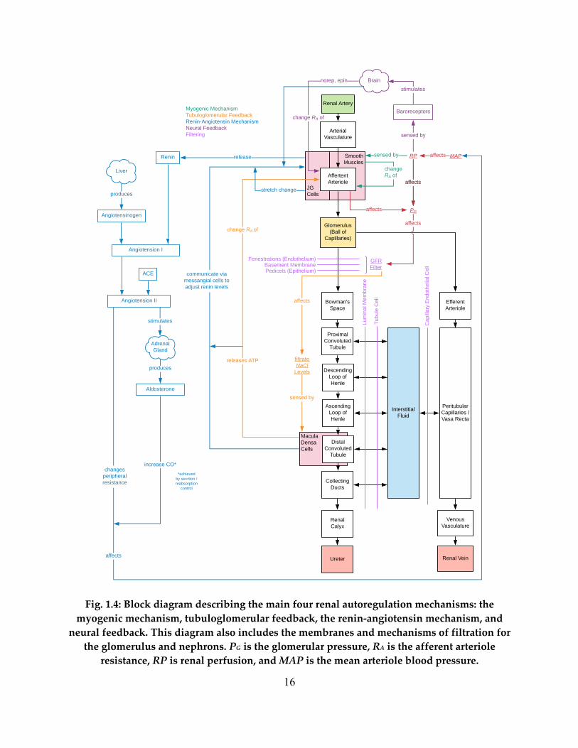
In Fig. 1.4, we see a block diagram of renal autoregulation, as well as the specific
membranes by which solutes and fluids must traverse at the glomerulus and nephron. Glomerular
filtration occurs across three distinct membranes, the fenestration level, the basement membrane,
and the pedicels. The fenestration level is purely filtration based on size as these fenestrations are
pores in the glomerular endothelium. The gel-like basement membrane is the least understood
membrane, but generally the agreed upon main function is to restrict small proteins from passing
via an electrical selectivity process. Generally speaking, no proteins should be filtered out by the
glomerulus. The final method of filtration are the podocytes or foot process that are interleaved,
with tiny slits that employ ultrafiltration.
Renal function is a highly controlled mechanism, one with several active concurrent
control loops. We begin with the myogenic response. This mechanism uses the smooth muscles
of the afferent arteriole to sense the pressure and subsequently change the resistance through the
afferent arteriole via constriction or dilation. The function of the myogenic response, along with
many of the other feedback mechanisms, is to control the flow of blood into the glomerulus and
hence maintain a healthy glomerular filtration rate (GFR).
The tubuloglomerular feedback mechanism accomplishes the same goal via a sensor in
the distal convoluted tubule. Here, the macula densa cells sense the salt concentration at this part
of the nephron. These cells, via the specialized JG (juxtaglomerular) cells that surround the
afferent arteriole will be used to stimulate the afferent arteriole to dilate or constrict depending
on the salt levels. Essentially, a change in GFR will eventually alter the salt levels in the distal
tubule and hence, sensing the salt levels here can be a direct indicator of GFR levels.

14
The most intricate renal autoregulation method is the renin-angiotensin mechanism. This
feedback involves several organs with a direct effect on the kidneys. In general, the kidneys
release renin which reacts with angiotensin that is produced by the liver and circulating
throughout the body. These reactants create angiotensin I. ACE inhibitors in the blood stream
will react with angiotensin I to form angiotensin II. Angiotensin II stimulates the adrenal glands
that then releases aldosterone. Both the angiotensin II and the aldosterone have the effect of
altering mean arterial pressure (MAP) and hence directly affecting renal perfusion. This
feedback mechanism will again alter the GFR via the change in renal perfusion. The beginning
of this process is the release of renin by the kidneys. The renin levels in the blood are controlled
by the kidneys and stimulation or inhibition of the release of renin is a direct function of the JG
cells. Hence, these JG cells are both the sensor for the renin-angiotensin mechanism and
tubuloglomerular feedback.
The final main control mechanism of the kidney is neural feedback. This feedback is not
directly controlled by the kidneys; however, it has a direct effect on the kidneys. As blood
pressure changes in the body, there will be a neural response brought on by the baroreceptors
that sense blood pressure, to constrict or dilate the vasculature in the body. This will directly
affect all the renal vasculature including, most importantly, the afferent arteriole that will directly
affect GFR.
These control mechanisms, along with the specialized nature of each segment allow for
the kidneys to maintain the fluid and electrolyte balance within the body, in a tightly controlled
range. While there are natural state fluctuations in the body (e.g., exercise, sleep, etc.), the
kidneys maintain a fairly constant GFR through all of this. When a segment of the kidneys

15
breaks down, then we see how the system responds in order to compensate. A breakdown of a
segment is an intrarenal disease and an important type of disease to study.
16
Fig. 1.4: Block diagram describing the main four renal autoregulation mechanisms: the myogenic mechanism, tubuloglomerular feedback, the renin-angiotensin mechanism, and
neural feedback. This diagram also includes the membranes and mechanisms of filtration for the glomerulus and nephrons. PG is the glomerular pressure, RA is the afferent arteriole
resistance, RP is renal perfusion, and MAP is the mean arteriole blood pressure.
JGCells
MaculaDensaCells
SmoothMuscles
Renal Artery
Arterial Vasculature
Affertent Arteriole
Glomerulus (Ball of
Capillaries)
Bowman's Space
Peritubular Capillaries / Vasa Recta
Interstitial Fluid
Venous Vasculature
Renal Vein
Proximal Convoluted
Tubule
Descending Loop of Henle
Ascending Loop of Henle
Distal Convoluted
Tubule
Collecting Ducts
Renal Calyx
Efferent Arteriole
Ureter
Fenestrations (Endothelium)Basement MembranePedicels (Epithelium)
changeRA of
RPsensed by
affects
affects
GFR Filter
PG
Lum
inal
Mem
bran
e
Tubu
le C
ell
Capi
llary
End
othe
lial C
ell
Myogenic MechanismTubuloglomerular FeedbackRenin-Angiotensin MechanismNeural FeedbackFiltering
affects
filtrate NaCl
Levels
sensed by
releases ATP
change RA of
affects
affects
communicate via messangial cells to adjust renin levels
Baroreceptors
sensed by
stimulatesnorep, epin
change RA of
Angiotensinogen
produces
Angiotension I
Renin release
Angiotension II
ACE
Liver
Brain
Adrenal Gland
stimulates
Aldosterone
produces
MAPaffects
stretch change
affects
changes peripheral resistance
increase CO**achieved
by secrtion / reabsorption
control
17
Chapter 2: Human Closed-Loop Kidney Model - Development,
Validation, & Analysis of Filtration Rate
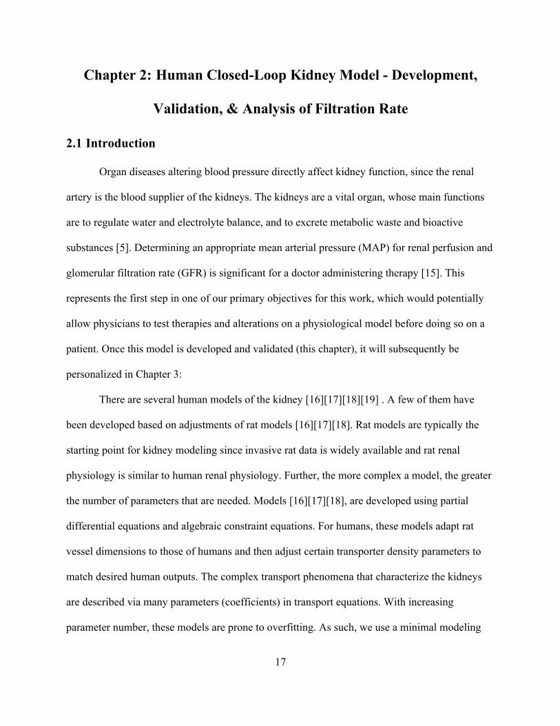
2.1 Introduction
Organ diseases altering blood pressure directly affect kidney function, since the renal
artery is the blood supplier of the kidneys. The kidneys are a vital organ, whose main functions
are to regulate water and electrolyte balance, and to excrete metabolic waste and bioactive
substances [5]. Determining an appropriate mean arterial pressure (MAP) for renal perfusion and
glomerular filtration rate (GFR) is significant for a doctor administering therapy [15]. This
represents the first step in one of our primary objectives for this work, which would potentially
allow physicians to test therapies and alterations on a physiological model before doing so on a
patient. Once this model is developed and validated (this chapter), it will subsequently be
personalized in Chapter 3:
There are several human models of the kidney [16][17][18][19] . A few of them have
been developed based on adjustments of rat models [16][17][18]. Rat models are typically the
starting point for kidney modeling since invasive rat data is widely available and rat renal
physiology is similar to human renal physiology. Further, the more complex a model, the greater
the number of parameters that are needed. Models [16][17][18], are developed using partial
differential equations and algebraic constraint equations. For humans, these models adapt rat
vessel dimensions to those of humans and then adjust certain transporter density parameters to
match desired human outputs. The complex transport phenomena that characterize the kidneys
are described via many parameters (coefficients) in transport equations. With increasing
parameter number, these models are prone to overfitting. As such, we use a minimal modeling

18
approach to ensure we are only using the necessary parameters to capture the structure of the
system without including parameters that cannot be validated.
Moss et al. [20] use a lumped parameter approach to dynamically model salt and fluid for
an entire rat kidney that reduces the number of parameters, but it is naturally not suitable for
human applications. Hallow et al. [18] modeled hyperabsorption in human diabetic kidneys,
focusing only on water and sodium transport. This model assumes negligible pressure drop
across the glomerulus, limiting the modeling of glomerular filtration. Another model from
Hallow and Gebremichael [21], describes the development of what they deem a core model, one
that can be used as a starting point for different studies and modeling endeavors. Their model is
similar to [18] in its use of physiologic parameters and modeling techniques, but may suffer from
possible overfitting due to a large number of parameters, 20 of which were simply tuned to make
the data fit their model. In this work, however, we have used a minimal number of parameters to
capture the relationship between mean arterial pressure and GFR. This was done to 1) avoid
potential overfitting and 2) due to the fact that invasive human measurements are needed to
validate internal states of the kidney are not widely available. Uttamsingh et al. [19] uses a
piecewise linear function adapted from a dog to model GFR as MAP changes in humans.
However, this approach is prohibitive in simulating impaired feedback and its effect on GFR.
Other models, as also mentioned in [7], are phenomenological models, which suffer from the
inability to determine which specific mechanistic segments of the kidneys have changed. The
parameters of a physiological model, on the other hand, when estimated, indicate specific kidney
insults, as diseases are represented by parameter alterations. Currently, the MDRD (Modification
of Diet in Renal Disease) is the method most used clinically in estimating GFR, as described in
[22]. It is also described here however, that this method is fraught with several shortcomings,

19
most notably its inaccuracy when GFR is above 60 mL/min/1.73m2, where it is expressed as mL
per min per square meter of body surface area. Therefore, in normal kidney function, this
equation is not reliable, and often labs simply report GFR above 60 mL/min/1.73m2 as normal.
Further, this equation has no predictive capabilities since the inputs to this equation (age, sex,
race, and creatinine) are not described functionally as related to blood pressure or other variables.
Another commonly used equation for estimating GFR is CKD-EPI (Chronic Kidney Disease
Epidemiology Collaboration). This equation is largely cited as being more accurate than the
MDRD equation [23]. However, with identical inputs, it has similar drawbacks in predicting
GFR as the MDRD equation.
We develop a human kidney model that uses a minimal set of adjustable parameters
while still capturing the essential physiology and avoids overfitting. Our steady-state, closed-
loop (i.e., with feedback signaling the afferent arteriole to dilate or constrict) model is a set of
algebraic equations produced by lumping several spatial locations together, thus minimizing our
equation set and parameters needed to run the model. In our model, we have several unknown
hydraulic resistance values along the nephron that are needed for simulation. We use
constrained trust-region optimization to validate the feasibility of the hydraulic resistance
parameter values throughout the nephron by ensuring that the dimensions estimated via the
optimization are physiologically sound. We calculate a pressure at the glomerulus, removing the
negligible pressure drop assumption across the glomerulus. In doing so, we are able to determine
GFR while making use of the Starling equation [5]. The model is validated against real human
data collected from ICU patients [24] and published studies [25]. This model can aid in renal
therapy via generation of a GFR-MAP relation and simulation of impaired feedback and
resistance change effects that mimic therapies. The model will further be personalized in the

20
following chapter, using a Levenberg-Marquardt optimization parameter estimation technique, to
determine the optimal therapy for an individual patient.
2.2 Methods
In this section, we will first describe some model assumptions, then the formulation of
model equations, parameters, and finally the physiological feedback mechanisms. Recall, we use
a first-principle, physiologic approach to modeling in order to understand the inner workings of
the system via physiological parameters. The equations of motion (derived in the sections to
follow) are a nonlinear algebraic system of equations comprising (2.1) – (2.12), are based on
kidney physiology, and are derived via continuity equations. The complete system of equations
can be seen in 2.2.5 and is solved with Newton’s method in MATLAB®.
With the aim of assessing the relation between blood pressure and GFR, we model the
movement of fluid throughout the kidney. The flow of fluid throughout the kidney can be altered
by tubuloglomerular feedback (TGF), which is a function of sodium concentration in the distal
tubule. Hence, since we model TGF, we also model the movement of sodium throughout the
nephron to be able to compute sodium concentrations in the distal tubule.
To accomplish this modeling task, the kidney is discretized into several spatial locations
(nodes) based on physiological reabsorption similarities between nodes. A schematic of the
considered spatial nodes, a linear graph [26], for a single nephron is shown in Fig. 2.1. with
arrows leading to node $ representing the reabsorption paths. Each node is characterized by a
hydraulic pressure and a sodium concentration. Fluid and sodium flow between nodes with
positive flows are indicated by the arrows in the figure. Similarly, to a linear graph, we can use
this node schematic to help derive the equations of motion. A single nephron is modeled first and
variables are then multiplied by two million [27] to give an indication of the total renal plasma

21
flow, GFR, and urine output. At each node, a mass conservation equation is developed,
describing the steady-state physics of the hydraulic pressure and sodium concentration at that
node.
Fig. 2.1: Kidney node schematic. Arrow directions indicate positive flow.
For healthy simulation (baseline) we use the following typical model input values: a
mean arterial pressure (MAP) of 90 mmHg, a ureter pressure of 0 mmHg, a venous pressure of 3
mmHg, and a venous sodium concentration of 140 mEq/L. We also assume that one tenth of the
cardiac output (CO) enters each kidney [5], with one two-millionth of this flow entering each
nephron. Renal plasma flow (RPF) is assumed to be 55% of the blood flow entering the kidney
Heart (H)
Renal Vein (V)
Glomerulus (G)
Bowman's Space (B)
Proximal Tubule (P)
Thin Descending Limb of Henle (N)
Thick Ascending Limb of Henle (K)
Distal Tubule (D)
Pre-Afferent Arteriole (A)
Post-Efferent Arteriole
(E)
Ureter (U)

22
and flowing into the pre-afferent arteriole node * in Fig. 2.1 [5]. Finally, we ensure that the sum
of total kidney urine flow and total kidney venous return must equal total kidney plasma flow.
2.2.1 Hydraulic Modeling
Fluid moves axially (through the vessels) due to a hydraulic pressure gradient. This flow
is determined by the hydraulic resistance parameter. The hydraulic resistance is a function of
fluid material property and vessel thickness. The flow of water between arbitrary nodes + and ,
via hydraulic pressure gradient is modeled by
-!"# = /! − /"1!"#
, (2.1)
where / is hydraulic pressure at node + or ,, 1!"# is hydraulic resistance from node + to ,, and
-!"# is hydraulic flow from + to ,.
Glomerular filtration modeling has consisted of either considering many capillaries in
parallel or lumping the entire set of capillaries into one compartment and assuming that pressure
and resistance drops across the glomerulus are negligible [28]. We calculate a pressure at the
glomerulus, thereby assuming there is a pressure drop across the glomerulus. We assume
negligible resistance along the glomerulus itself due to the large number of capillaries in parallel
(effectively reducing resistance to a negligible number). At the second and third nodes of Fig.
2.1, the glomerular filtration (between nodes 3 and 4) is modeled via the Starling equation as
seen in (2.2) below, since here there is an oncotic pressure due to the proteins in the blood. This
equation is equivalent to hydraulic fluid flow (where the glomerular filtration coefficient is
included in the resistance term 1$%# ), with an added term for the oncotic pressures, 5. This
oncotic pressure is due to proteins that are not filtered at the glomerulus and remain in the blood
vessels and therefore we assume a reflection coefficient of unity for this oncotic pressure. The
equation used for fluid flow between nodes 3 and 4 is

23
-$%& = /$ − /% − 5$%
1$%#. (2.2)
A typical value of the oncotic pressure between the glomerulus and Bowman’s space is 5$% =
30 mmHg [27] is used. The remaining fluid flow equations are derived from (2.2) when there
are no proteins separated by a membrane.
In subsequent nodes, fluid is reabsorbed in the bloodstream along the nephron from the
proximal tubule (6), thin descending limb of Henle (7), and the distal tubule (8) as shown in
Fig. 2.1 by the arrows going into node $. We follow the assumption that the cellular walls of the
thick ascending limb of Henle (node 9) are impermeable to water and therefore no fluid is
reabsorbed from 9. We define a reabsorption fraction at each node where fluid is reabsorbed, as
a percentage of the incoming axial flow. This transverse reabsorption fluid flow from an
arbitrary node , back to the veins, $, is therefore described by
-"'( = :"# ⋅ -!"# , (2.3)
where :"# is the fluid reabsorption fraction at node ,, and -!"# is the axial flow (along the
nephron) into node , from node +. The reabsorption fractions of 6 and 8 are nearly constant,
regardless of fluid flow, in healthy cases, as described by [19]. For node 6, a constant value of
0.75 is used for the reabsorption fraction due to the glomerulotubular balance, where
reabsorption fractions of fluid and sodium are approximately equal and invariant to GFR. For 8,
a constant value of 0.95 is used for the reabsorption fraction, which changes with antidiuretic
hormone levels, but not with fluid flow, into 8. A constant antidiuretic hormone level
corresponding to a 0.95 reabsorption fraction of water from node 8 was used. [19]. For node 7,
the reabsorption fraction is an inverse function of fluid flow into 7 given by [19] as
:)# = 0.65 − 0.01-*)# . (2.4)

24
2.2.2 Sodium Modeling
As previously mentioned, we model sodium in the nephron in order to model TGF. Since
sodium is freely filtered at the glomerulus, we assume that the sodium concentration at
Bowman’s space (node4) and at the renal veins (node $) are equal.
Axial flow of sodium along the tubule is due to advection, which is the movement of
solutes by bulk fluid flow. Advective flow between nodes + and , is modeled via this equation,
?!"+ = -!"# ⋅ @!,- (2.5)
where @!,- is the sodium concentration at node + and -!"# is the hydraulic flow between nodes +
and ,.
Sodium reabsorption flow is modeled similarly to fluid reabsorption, in that we define
reabsorption fractions for each node along the nephron. The transverse flow of sodium from an
arbitrary node , back to the veins, $, is therefore described by
?"'( = :",- ⋅ ?!"+ , (2.6)
where :",- is the sodium reabsorption fraction at node ,. The cellular walls at the thin ascending
limb of Henle (node 7) are impermeable to sodium and therefore the reabsorption fraction there
is zero. For node 6, we again use 0.75, as fluid and sodium are reabsorbed at almost one to one
ratio. According to [19], the reabsorption fraction at the thick ascending limb of Henle (node 9)
is approximately invariant to the flow into node 9 and approximately equal to 0.80 and as such
:.,- = 0.8. At node 8, the reabsorption fraction is determined by another renal feedback
mechanism, the renin-angiotensin mechanism where the sodium reabsorption fraction is
modulated by aldosterone blood levels, as outlined by Uttamsingh et al. [19]. This is given by an
inverse sigmoidal function of sodium flow into 8,

25
:.)+ =0.2268
1 + C/01!"# 20.04+ 0.7316. (2.7)
2.2.3 Parameter Estimation: Hydraulic Resistance
Axial fluid flows are characterized by hydraulic resistances. Hydraulic resistances of the
axial flows are calculated via two methods. Method 1 uses the Poiseuille equation assuming
laminar flow where the resistance between nodes + and ,, is given by
1!"# = 8DE 5:5,
(2.8)
where D is fluid viscosity, and E and : are the average length and radii of nodes + and ,,
respectively. Given the variability in human nephron dimensions, even between neighboring
nephrons, calculating resistances via Method 1 may not yield resistances that achieve
physiologically accurate pressures throughout the nephron. For instance, small changes in radius
will produce large changes in resistance, as the radius is raised to the fourth power in (2.8). By
assuming healthy pressures, a GFR of 120 mL/min [27], healthy reabsorption fractions as
discussed above, and a resistance from 3 to 4 of 1$%# = 100 s/mL/mmHg, the hydraulic
resistances can also be calculated directly from the continuity equations (conservation of mass),
which defines Method 2. The resistances via Methods 1 and 2 ought to be identical, naturally.
We then use optimization techniques (described below) to find feasible dimensions (lengths and
radii) of the vessels. Subsequent resistances could then be calculated using (2.8). These
dimensions found via the optimization iteratively solving the system of equation should be
within a physiologically feasible range.
In Method 2, all axial hydraulic resistances (including those along the tubule, excluding
1$%# ) were calculated using a set of physiologically reasonable pressures that are given in Table
2.1. The afferent arteriole resistance (16$# ) is modulated by tubuloglomerular feedback as well as

26
the ascending and descending myogenic feedback mechanisms, and hence 16$# varies with
pressure. The 16$# calculated from the equations is after feedback modulation. The baseline value
of 16$# , in the absence of feedback, was estimated from [29] to be 17# = 2.78 × 10⁸
s/mL/mmHg.
Table 2.1: Pressure Values Used in Resistance Calculation.
Node H (mmHg) Notes * 77 Estimated within feasible range 3 55 Given from [27] I 17 Estimated from [5] 4 15 Given from [27] 6 10
Pressure from 6 to 8 decreases along tubule between 15 mmHg at 4 and 0 mmHg at J
7 7 9 6 8 4
Our goal is to determine feasible scaling factors of the lengths and radii that will be used
to calculate resistances via Method 1. These calculated resistances will then be used in
simulation using baseline parameters, outputting the prescribed pressures. The iterative
constrained optimization technique minimized the sum of the squares of the difference between
resistances estimated from Method 1 (which uses the scaling factors to calculate resistance) and
Method 2 (which are the true resistances) by estimating the scaling factors. Baseline dimensions
were taken from Layton and Layton [16]. These scaling factors (outputs of the optimization) are
nondimensional constants multiplying baseline lengths and radii, bound to a range between 0.7
to 1.2, with an initial value of 1. This range represents varying nephron sizes in humans [30].
The optimization results in Table 2.2 show a feasible solution, with a possible local
minimum. In this problem, we were more interested in feasibility (satisfying constraints) rather
than optimality, for lengths and radii (and thus a global minimum) was not necessary to find.

27
These optimized parameters (scaling factors) are then used to calculate resistances, assuming
Poiseuille flow with (2.8), which will induce feasible pressures throughout the system at a
healthy MAP = 90 mmHg.
Table 2.2: Resistance Parameter Estimation Results. Lengths and radii from the literature and the optimization algorithm are in cm. The literature values of the dimensions are also
presented and given such that the value from the literature multiplied by the scaling is the optimized value. Resistances assuming Poiseuille flow calculated from values in the
literature [16] before and after optimization (s/mL/mmHg) are also shown.
Node Lengths Radii
Branch Poiseuille Resistance
Optimized Resistance Literature
[16] Optimized Scaling Literature [16] Optimized Scaling
! 1.7 2.0024 1.178 0.0019 0.0013 0.707 ,! 1.06 × 10! 5.00 × 10! 0 0.32 0.3838 1.199 0.0013 0.0009 0.702 !0 2.51 × 10! 12.0 × 10! 1 1 0.7 0.700 0.0013 0.0013 0.982 01 3.77 × 10! 6.15 × 10! 2 2 2.3947 1.197 0.0010 0.0011 1.116 12 14.0 × 10! 12.3 × 10!
The resulting resistances in Table 2.2 are, in some instances, much larger than those
estimated from the original dimensions. However, since all lengths and radii are bounded
between 0.7 and 1.2 times their original values, they still represent plausible resistances for a
human. The average percent error between resistances calculated from continuity equations
versus those calculated from optimization is 5.2 × 1028% indicating a good fit between the
optimized values. Using the resistances in Table 2.2, we arrive at accurate pressures throughout
the system that match the prescribed pressures in Table 2.1.
In addition to finding the resistances via optimization, we needed to find the hydraulic
resistance from the heart (node N) to the pre-afferent arteriole (node *) for simulations where
MAP is varied, since we could no longer use a predefined renal plasma flow, because this flow
varies with MAP. A pressure drop from the heart (node N) to node * was set to 13 mmHg in
accordance with [31]. With this pressure drop and a baseline cardiac output of 5.5 L/min at an

28
MAP of 90 mmHg, the resistance from heart to pre-afferent arterioles (196# ) was calculated to be
2.58 × 10⁸ s/mL/mmHg by rearranging (2.1) to solve for the resistance.
2.2.4 Feedback Mechanisms
Since patient measurements typically occur at intervals longer than the transient response
of the kidney, we are only interested in GFR after this transient response. As such, we adopt the
steady-state feedback equations of [32], implemented by [33]. They included tubuloglomerular
feedback (TGF) and descending and ascending myogenic feedback mechanisms. A feedback
diagram is presented in Fig. 2.2. As shown, all feedback mechanisms share a common actuator
that is the afferent arteriole muscles that change 16$# by constricting or dilating.
Fig. 2.2: Feedback diagram for tubuloglomerular feedback and descending and ascending myogenic mechanisms. Model inputs include mean arterial pressure, ureter pressure, venous
pressure and sodium concentration.
However, each controller has a different sensed input (located in the feedback paths in
Fig. 2.2). TGF (2.10) senses @.,- and imposes an additional resistance 1:$;# on the baseline
resistance of 16$# , denoted by 17#, as @.,- decreases. The descending myogenic mechanism (MD)
senses pre-afferent arteriole pressure and imposes an additional resistance 1<.# when this
pressure rises above 67 mmHg, as seen in (2.11) below. Beyond 67 mmHg, 1<.# continually
Renal Model
Distal sodium concentration sensing
Pre afferent arteriole pressure sensing
+ -
+ -
Ascending Myogenic Mechanism Controller
Descending Myogenic Mechanism Controller
Tubuloglomerular Feedback Mechanism Controller
+++ GFR
Actuator (muscles of afferent arteriole)
Model Inputs
Desired pre afferent pressure
Desired distal sodium
concentration
++

29
increases, linearly with pre-afferent pressure, as the vessel continues to constrict. The ascending
myogenic mechanism (MA) senses afferent arteriole resistances (determined by the descending
myogenic mechanism and TGF, since MD is a function of TGF) and imposes yet another
resistance 1<6# , as shown in (2.12). The total resistance is hence given by the combined additive
effect of all feedback mechanisms as
16$# = 17# + 1:$;# + 1<.# + 1<6# (2.9)
with,
1:$;# = 0.15051 + C/5.=25>?"$%4
1<.# = 0.5 ⋅ O17# + 1$@# + 1:$;# P ⋅ Q/667 − 1R ⋅ N(/6 − 67)
1<6# = 0.5 ⋅ 17# + 1<.#1$@#
,
(2.10) (2.11) (2.12)
where1$@# is the hydraulic resistance from glomerulus to post-efferent arteriole and N(/6 − 67)
is the Heaviside function that is 0 when /6 is below 67 mmHg and 1 otherwise. It can be seen
that (2.12) is a function of 1<.# and subsequently 1:$;# as well. Equations (2.10) – (2.12) are
multiplied by a feedback gain. When these gains are zeros, the system is open loop. For a healthy
person, these gains are ones.
2.2.5 Summary of Equations
Considering each node in the system, we can write the continuity equations for both fluid
and sodium. Beginning with fluid, we have the following equations,
Node Continuity Equation
4 /A − /B1AB#
+ 3U1/W = 0 (2.13)
6 /A − /B1AB#
− /B − /,1B,#− :*
#(/A − /B)1AB#
= 0 (2.14)

30
7 /B − /,1B,#
− /, − /C1,C#− :)&# ⋅ /B − /,1B,#
+ :)'# ⋅(/B − /,)D
O1B,# PD= 0 (2.15)
9 /, − /C1,C#
− /C − /E1CE#= 0 (2.16)
8 /C − /E1CE#
− /E − /F1EG#− :.# ⋅
/C − /E1CE#
= 0 (2.17)
* MAP − /H1IHB# − -6$ = 0 (2.18)
3 -6$ −/J − /K1JK#
+ 3U1/W = 0 (2.19)
I -6$ −/J − /K1JK#
+ 3U1/W = 0 (2.20)
where W is the number of nephrons, : are the reabsorption fraction parameters defined earlier,
and all other variables and parameters follow the notation in the previous equations. The fluid
flows, GFR (glomerular filtration rate), UO (urine output), and -6$ are defined as,
3U1 = W ⋅ /A − /J + 5JA1JA# (2.21)
JX = W ⋅ @E(/E − /F)1.F#
(2.22)
-6$= (/H − /J)
⋅
⎝
⎜⎜⎜⎜⎜⎜⎜⎛1IHB# +
\:$;'expO\:$;& − \:$;(@EP + 1
+\<.N(/H − 67) Q/H67 − 1R
`1JK# + a1IHB# +\:$;'
expO\:$;& − \:$;(@EP + 1b +
\<6\:$;'a1IHB# + \<.\<6\:$;'N(/H − 67) c/H67 − 1d ⋅
`1JK# + a1IHB# + \:$;'expO\:$;& − \:$;(@EP + 1
b
1JK# expO\:$;& − \:$;(@EP +1JK# ⎠
⎟⎟⎟⎟⎟⎟⎟⎞
2L
(2.23)
where N is the Heaviside function and \ are feedback specific parameters defined in (2.10)-
(2.12). Recall that the fluid flow -6$ is flow from the pre-afferent arteriole to the glomerulus and
is heavily modulated by autoregulation. Thus, (2.23) is derived by substituting (2.10) – (2.12)

31
into (2.1). And hence, we see /H and @E appear in (2.23) since they are the feedback inputs for
the descending myogenic, ascending myogenic, and TGF.
For all nodes concerning sodium, we have the following equations,
Node Continuity Equation
6 @' (/A − /B)
1AB#− @B
(/B − /,)1B,#
− :*M ⋅@'(/A − /B)
1AB#= 0 (2.24)
7 @B(/B − /,)
1B,#− @,
(/, − /C)1,C#
= 0 (2.25)
9 @,(/, − /C)
1,C#− @C
(/C − /E)1CE#
− :NM ⋅@,(/, − /C)
1,C#= 0 (2.26)
8
@C(/C − /E)1CE#
− JXW − :.(M −:.(M − :.)M
exp `:.'M :.&
M + :.'M ⋅ @C(/C − /E)1CE#
b + 1
⋅ @C(/C − /E)1CE#
= 0
(2.27)
Note that since we are assuming sodium concentration at Bowman’s space is equivalent to
venous sodium concentration (a physiologically sound assumption since sodium is freely
filtered), we only require equations for the four nephron component nodes in order to solve for
all sodium concentration values.
2.3 Results & Discussion
2.3.1 Model Validation
The model is validated against real patient data as well as other models in the literature.
As will be detailed in the results below, we first compare our model outputs to the model outputs
from [16] and [19]. We then validate against patient data by comparing model generated GFR vs.

32
MAP to those of five intensive care unit patients with diagnoses unlikely to impact kidney
function. Finally, we compare the same GFR vs. MAP curve to the data from 20 patients (across
a large range of ages) reported in [25] over a two-hour study. None of these patients had clinical
evidence of primary renal disease.
We simulated the model under healthy conditions at MAP = 90 mmHg (/! in (2.1) for
the continuity equation at node *) for healthy cases and solve for all pressures, flows, and
sodium concentrations at and between the nodes in Fig. 2.1. Sodium concentrations along the
tubule were compared to Layton and Layton’s continuous steady-state model [16] in Fig. 2.3a.
As shown, the values are close in magnitude. This is a good indication that the concentrations of
sodium in the tubule are physiologically sound. Of note, our model lumps the distal tubule and
collecting duct into one node as also seen in [19], and therefore we see, in Fig. 2.3a, our sodium
concentration at 8 slightly differ from [16]. However, we observed little impact of the length of
the 8 node on the resulting sodium concentration and our model’s determination of GFR.

33
(a)
(b)
0 1 2 3 4 5 6Distance from Bowman's Space (cm)
0
50
100
150
200
250
300
350
Sodi
um C
once
ntra
tion
(mEq
/L)
B P
N
K D
ModelLayton and Layton
0
50
100
150
200
250
300
350
Sodi
um C
once
ntra
tion
(mEq
/L)
B P N K DNephron Nodes
MAP = 54.0 mmHgMAP = 90.0 mmHgMAP = 126.0 mmHgMAP = 162.0 mmHg

34
Fig. 2.3: Model sodium concentration values along the tubule compared to [16] and over varied MAP inputs ranging from 54 to 180 mmHg.
Flow values of fluid and sodium between several nodes are compared to Uttamsingh et
al. [19] in Table 2.3, with percent differences reported. Our baseline (no parameter alterations)
simulation results indicate good matching to those of Uttamsingh et al., with an average percent
difference of 7.7%. Our model explicitly includes resistances and pressures and uses the Starling
equation, rather than the piecewise linear function used by Uttamsingh et al., for calculation of
GFR via (2.2), allowing us to simulate impaired feedback and observe subsequent changes in
GFR, as presented in 2.3.2.
Table 2.3: Model output flows.
Fluid flows in mL/min. Branch Uttamsingh et al. [19] Model % Difference 34 125 115.47 7.62 67 31.25 28.87 7.62 8J 1 0.850 15.1 6$ 93.75 86.61 7.62 7$ 10.55 10.43 1.12 8$ 19.7 17.56 10.9
(a)
Sodium flows in mL/min. Branch Uttamsingh et al. [19] Model % Difference 67 4.44 4.04 8.97 98 0.89 0.50 9.26 6$ 13.3 12.1 8.83 9$ 3.55 3.23 8.91 8$ 0.76 0.75 0.52
(b)
After validating our model against other models, we then varied MAP over the range of
54 to 180 mmHg in increments of 10% of the baseline (90 mmHg). The effect of MAP on
sodium concentration along the nephron can be seen in Fig. 2.3b. With the rise in MAP, RPF

35
also rises as given by (2.1). The increased RPF decreases fluid reabsorption from 7 since the
reabsorption fraction and fluid flow into node 7 are inversely related, as described in (2.4).
Therefore, @),- decreases as MAP increases, especially since sodium mass does not change in 7
either, due to the impermeability of the tubule to sodium at this location.
At node 8, sodium concentration increases with MAP. This is due to the inverse
relationship between sodium reabsorption and sodium flow into 8 as described in (2.7). This is
expected, since TGF increases afferent arteriole resistance to decrease RPF and GFR when @.,-
is high.
GFR was also analyzed during a variation of MAP as shown in Fig. 2.4a. A spline
interpolation was inserted between simulation points to generate a continuous curve. A healthy
GFR range of 90 to 120 mL/min is highlighted between two horizontal dotted lines. Additional
simulations are shown where different feedback mechanisms were disabled in Fig. 2.4a. As can
be seen in the open loop system (dashed line with open square markers), after 85 mmHg, GFR is
already beyond the healthy limit of 120 mL/min (now in the region of hyperfiltration) and
climbs rapidly (almost linearly) as MAP increases. The descending (solid line with open square
markers) and ascending myogenic mechanism are effectively inactive below MAP = 80 mmHg
and beyond this point, they begin to increase 16$# continually as MAP increases. This increase in
16$# decreases GFR for a given MAP. TGF (dotted line with open square markers) becomes less
effective, saturating to a maximum 1:$;# value beyond which increased MAP values are no
longer controlled by this mechanism, as shown by the line’s change in slope with sufficiently
large MAP. The ascending myogenic response is not simulated without the descending myogenic
response and TGF, as 1<6# would be zero without the TGF. The descending myogenic response
is simulated without TGF where 1:$;# = 0, in (2.11). Uttamsingh et al.’s [19] equation (solid

36
line with no markers) for GFR as MAP changes and our curve (solid line with markers, with all
feedback mechanisms enabled) match very well between 80 and 100 mmHg, the agreed-upon
healthy range of MAP. The ascending myogenic mechanism has the effect of decreasing GFR
with increased MAP beyond 80 mmHg, as demonstrated in [32]. As such, including the
ascending myogenic mechanism causes the GFR vs. MAP curve to flatten or increase GFR much
less for further MAP increases. This is an important component for regulating and maintaining
GFR for individuals.
(a)
60 80 100 120 140 160 180Mean Arterial Pressure (mmHg)
0
50
100
150
200
250
300
Glo
mer
ular
Filtr
atio
n Ra
te (m
L/m
in)
Healthy GFR Range
Uttamsingh et al.Open LoopMDTGFMD + TGFMD + TGF + MA
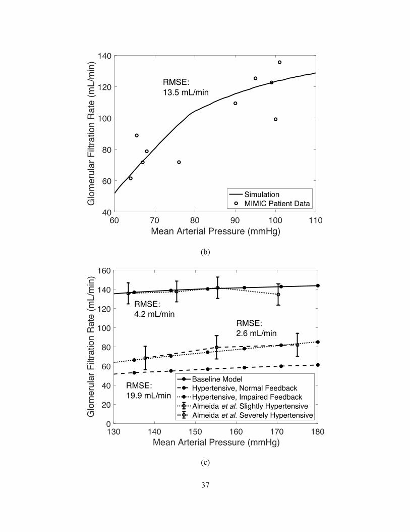
37
(b)
(c)
60 70 80 90 100 110Mean Arterial Pressure (mmHg)
40
60
80
100
120
140
Glo
mer
ular
Filt
ratio
n R
ate
(mL/
min
)RMSE:13.5 mL/min
SimulationMIMIC Patient Data
130 140 150 160 170 180Mean Arterial Pressure (mmHg)
0
20
40
60
80
100
120
140
160
Glo
mer
ular
Filt
ratio
n R
ate
(mL/
min
)
RMSE:4.2 mL/min
RMSE:2.6 mL/min
RMSE:19.9 mL/min
Baseline ModelHypertensive, Normal FeedbackHypertensive, Impaired FeedbackAlmeida et al. Slightly HypertensiveAlmeida et al. Severely Hypertensive

38
Fig. 2.4: Glomerular filtration rate plotted as input MAP is varied: (a) under varying controllers active and compared to Uttamsingh et al. [19] simulation, (b) compared to
Massachusetts’ ICU hospi’al's patient data [24], and (c) in slightly and severely hypertensive cases as compared to real human data from Almeida et al. [25]. RMSE is root mean squared
error. Descending myogenic mechanism (MD), ascending myogenic mechanism (MA), tubuloglomerular feedback (TGF)
We next compared model-computed GFR to the GFR calculated using patient data from
the MIMIC database [24] and utilizing the widely used Modification of Diet in Renal Disease
(MDRD) formula [34] after removing the GFR normalization by patient body surface area.
MIMIC was chosen since it is a large and a diverse population database. It is also widely used in
the research community and easily accessible. The database also includes multiple measurements
from a single patient, at different times and for different MAP values, rather than aggregated or
averaged population data only. This type of time-series data is needed to validate model outputs
for a single patient, having multiple inputs. All ICU stays are considered separately – even if the
stay is a readmission of the same patient. Because we modeled a healthy individual, we want to
first validate on healthy patients. Since most patients in the MIMIC ICU data are critically ill, we
sought to find relatively healthier patients, i.e., those with no acute or chronic kidney problems,
and then filter out those with other kidney, heart, or severe illnesses that could impact kidney
function. Patients were included according to the criteria described in the chart of Fig. 2.5.

39
Fig. 2.5: Patient inclusion criteria from MIMIC database. After removing patients with insufficient data for calculating a KDIGO (Kidney Disease Improving Global Outcomes) stage of 0, indicating no acute kidney injury, we had a set of 12,666 unique ICU stay IDs (identification number for each stay). Patients were further filtered from the database by retaining only those meeting the following criteria: patients who have height and weight
records in order to remove GFR body surface area normalization in the data (419 remaining), patients who have not undergone surgery during a stay, which may affect GFR (293
remaining), patients who have not passed away during a stay (146 remaining), patients without diseases such as diabetes, cancer, pancreatitis, etc. (127 remaining), patients with
diagnoses that would most likely not affect kidney function (5 remaining).
From the remaining patients, we have a total of 10 ten points for validation. These data
points span a large MAP range and will hence validate the model for low and high MAP values.
Four of the patients remaining were male. The mean age was 34.2, with standard deviation of
15.5. The mean BMI (body mass index) was 21.4, with standard deviation 4.9. The diagnoses
419 PatientsHeight and Weight Records
293 PatientsNo Surgery
146 PatientsNo Expire Flag
127 PatientsNo Comorbidities
5 PatientsNo Kidney Affecting
Diseases
12,666 PatientsKDIGO Stage 0
61,532 PatientsMIMIC Database

40
were altered mental status, diaphragmatic injury, and abnormal head CT. It is important to note
that all patients were under the age of 60, and patients, with the exception of one, were within a
healthy BMI (body-mass-index) of 18.5 and 24.9. These two observations are important, as age
can greatly affect GFR, generally diminishing with age, and a large BMI will result in a larger
GFR than for a similar patient with a lower BMI since the MDRD equation, for calculating GFR,
is normalized by body surface area, whereas our model outputs are not.
The associated blood pressure and GFR measurements were plotted for these ICU stay
IDs against the simulated curve that can be seen in Fig. 2.4b above. Several patients had more
than one measurement of blood pressure and GFR, hence we see more than 5 data points, even
though we had only 5 patients. The data does not fit our curve perfectly, as is expected without
manual fitting or model fine-tuning, but it does show the general shape and magnitude of our
curve. GFR can be altered by many factors that are not captured in the general model and
therefore a more personalized model with parameters reflecting each patient would better fit the
data for each patient. We observe an RMSE (root mean squared error) of all the data of 13.5
mL/min. This is a reasonable number considering the data is from 5 unique ICU stay IDs and
there are healthy variations between patients in general due to natural variations in parameter
values. We note also that the data fits the curve reasonably well in regions where feedback is not
active (below MAP = 80 mmHg) and areas where feedback is active (above MAP = 80 mmHg).
This gives credence to the model when fitting low pressure MAP input data where renal
autoregulation is largely inactive. It also shows that the model can fit high pressure MAP input
data where renal autoregulation is vital for maintaining GFR.
The purpose of this validation against real patient data is to ensure that the model is able
to capture the steady-state response of GFR to changes in MAP. With a low dataset number, we

41
cannot expect to claim overarching statistical conclusions on the model fit to patient data.
However, we can claim the model is capable of describing this relationship within a reasonable
range (15 mL/min GFR RMSE). Patient parameters can vary greatly from person to person as
seen in [10], [35], and [36], describing the changes in nephron number, glomerular resistance,
and renal autoregulation based on patient demographics alone. It is important to note that the
validation data using healthy kidneys would correspond to normal parameters values, and this
would be the first validation step, while altered parameters correspond to diseased kidneys. As
such, a personalized patient-to-model fit would require parameter adjustment, even for healthy
patients. As BMI increases, parameters in the model will change. This is due to the link between
obesity and structural changes to the kidney that can cause decreased glomerular resistance and
tubular flow in the loop of Henle [11], [37]. In the Analysis section we will observe how
changing parameter values affects the model outputs. The current model can only describe
certain clinical conditions. To address others, we would need to change several parameters to
reflect healthy or diseased states of the patient. These parameters include aldosterone and
antidiuretic hormone levels, glomerulotubular balance, reabsorption fractions, glomerular
filtration resistances, and/or resistances. Several of these parameters, for instance, will change for
diseases such as tubular necrosis or glomerulonephritis as described in [38].
We investigated the effect of administration of vasodilators in patients where there is a
need to reduce MAP without negatively affecting GFR. We used real patient data from [25],
where slightly and severely hypertensive patients were administered a stepwise infusion of
sodium nitroprusside (SNP) to target acute blood pressure reductions. The slightly hypertensive
patient group consisted of four men and six women with a mean age of 41.7±3.8 years (16-55
range), while the severely hypertensive patient group comprised four men and six women with
42
a mean age of 38.5±4.3 years (15-58 range). We simulate SNP infusions as a change (reduction)
in MAP. We plotted the collected data versus our model results in Fig. 2.4c. In the case of slight
hypertension (dotted error bar line), our model (solid line), without any adjustment to vascular
resistances or feedback gains, fits the data well with an RMSE of 4.2 mL/min. To model severe
hypertension, a sixfold increase of all vascular resistances (196# , 16$# , 1$@# , and 1@'# ),
corresponding to a decrease in vascular radii by 0.55 times, was used. Almeida et al. [25] notes
that the measurements of the severely hypertensive patients suggest that their feedback
mechanisms are affected. Impaired feedback was then modeled by a decrease in feedback gains
(multiplication by 0.5) in all three feedback mechanisms described in (2.9). After adjustments to
vascular resistances and feedback gains, the model (dotted line) accurately represents the
severely hypertensive patient GFR data (dashed error bar line) with an RMSE of 2.6 mL/min,
shown in Fig. 2.4c. In the case where vascular resistances are increased and feedback is not
modulated (dashed line), the slope of the curve is nearly identical to the baseline curve, but the
GFR values are too low to match the patient data having only an RMSE of 19.9 mL/min. This is
expected as the feedback mechanisms affect the slope of the GFR vs. MAP curve mostly.
Feedback has a dampening effect on GFR as MAP changes, flattening the curve with increased
feedback modulation as can be seen in Fig. 2.4a. This reinforces the hypothesis of Almeida et al.
[25] that the feedback is impaired in severe hypertension, since here the model more closely
matches severely hypertensive data after feedback modulation (Fig. 2.4c).
2.3.2 Model Analysis
We then conducted a sensitivity analysis to study how GFR and sodium concentration
along the tubule are affected when vascular resistances and feedback gains are altered. Over a
vascular resistance range of 1 to 8 times the baseline value, signifying worsening hypertension,

43
we simulated the system over a range of MAP values. We also varied feedback gains over a
range of 0 to 2 for the same MAP range, independently, simulating instances where feedback is
altered, such as in hypertension. Results of varied vascular resistances and feedback gains are in
Fig. 2.6, where a is a gain by which the vascular resistances or feedback gains were altered. For
Fig. 2.6a and Fig. 2.6b, observing GFR, the dotted lines are individual simulations, and the solid
lines delineate the region covered by the simulations.
(a)
60 80 100 120 140 160 180Mean Arterial Pressure (mmHg)
0
50
100
150
200
250
300
350
Glo
mer
ular
Filt
ratio
n R
ate
(mL/
min
)
Baseline = 1
= 8

44
(b)
(c)
60 80 100 120 140 160 180Mean Arterial Pressure (mmHg)
0
50
100
150
200
250
300
350
Glo
mer
ular
Filtr
atio
n Ra
te (m
L/m
in) = 0
(OpenLoop)
Baseline = 1
= 2
0
50
100
150
200
250
300
350
Sodi
um C
once
ntra
tion
(mEq
/L)
B P N K DNephron Nodes
= 1 = 2 = 3 = 8
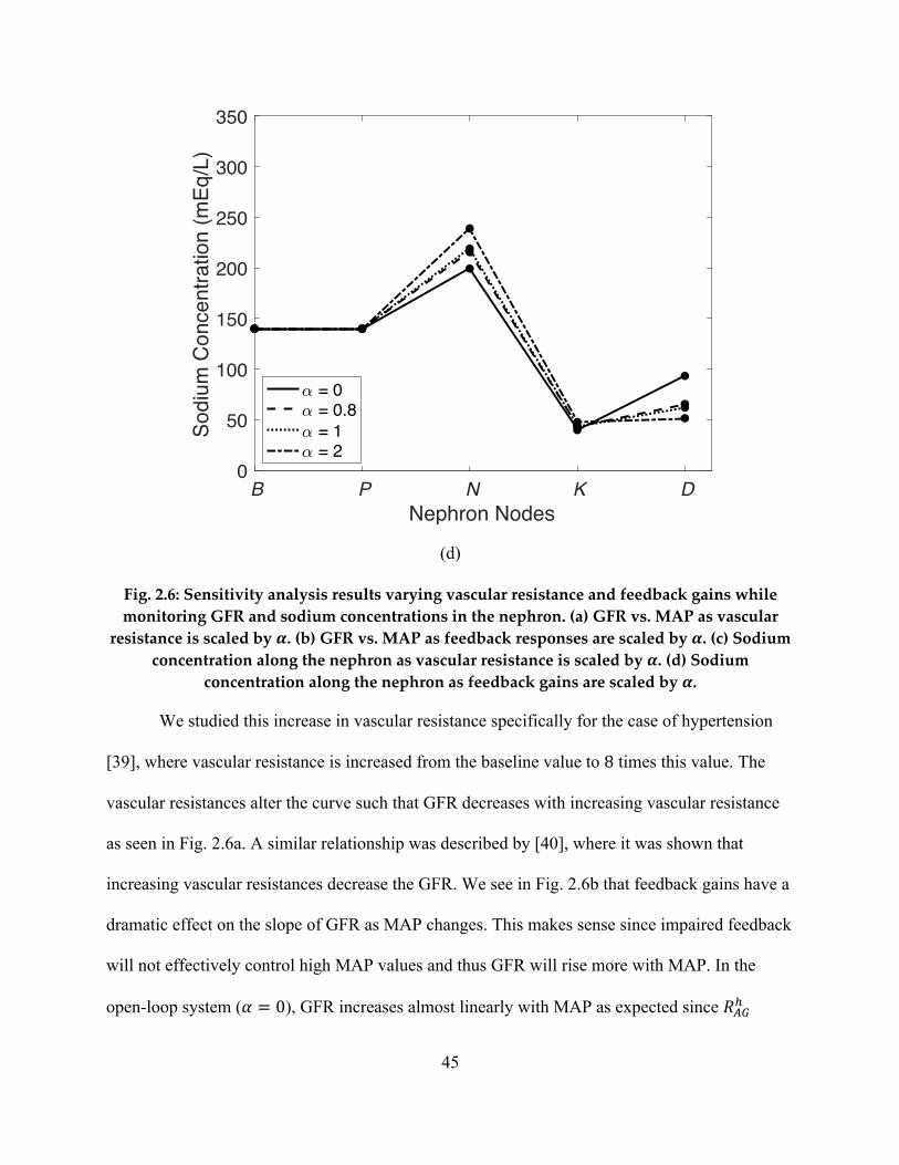
45
(d)
Fig. 2.6: Sensitivity analysis results varying vascular resistance and feedback gains while monitoring GFR and sodium concentrations in the nephron. (a) GFR vs. MAP as vascular
resistance is scaled by !. (b) GFR vs. MAP as feedback responses are scaled by !. (c) Sodium concentration along the nephron as vascular resistance is scaled by !. (d) Sodium
concentration along the nephron as feedback gains are scaled by !.
We studied this increase in vascular resistance specifically for the case of hypertension
[39], where vascular resistance is increased from the baseline value to 8 times this value. The
vascular resistances alter the curve such that GFR decreases with increasing vascular resistance
as seen in Fig. 2.6a. A similar relationship was described by [40], where it was shown that
increasing vascular resistances decrease the GFR. We see in Fig. 2.6b that feedback gains have a
dramatic effect on the slope of GFR as MAP changes. This makes sense since impaired feedback
will not effectively control high MAP values and thus GFR will rise more with MAP. In the
open-loop system (a = 0), GFR increases almost linearly with MAP as expected since 16$#
0
50
100
150
200
250
300
350
Sodi
um C
once
ntra
tion
(mEq
/L)
B P N K DNephron Nodes
= 0 = 0.8 = 1 = 2

46
(modulated by the feedback) is severely decreased, as also seen in Fig. 2.4a. This reinforces the
importance of feedback to maintain GFR during high MAP periods. Overall, GFR is more
sensitive to impaired feedback as compared to changes in vascular resistances as seen by the
larger changes in GFR from equivalent changes to vascular resistances or feedback gains in Fig.
2.6a and Fig. 2.6b. This is an important fact to note since this implies that diseases or therapies
that alter renal autoregulation, as opposed to vascular resistance, will impact GFR more.
We also studied how the sodium concentration, along the tubule, is affected by changes
in vascular resistances and feedback gains, specifically at MAP = 90 mmHg. Typically, sodium
concentration is not measured in the nephron, hence the importance of this study. Results can be
seen in Fig. 2.6c and Fig. 2.6d. The largest impacted sodium concentrations occur in the
descending limb of Henle in response to changed vascular resistances and feedback gains.
Sodium concentration in the distal tubule is also largely affected by feedback gain changes via
TGF so it makes sense that sodium concentration would vary significantly in the same direction
as this change. This noninvasive observation from the simulation is important because sodium is
pivotal in maintaining the fluid-electrolyte balance in the body.
As the vascular resistance increases, @),- (concentration of sodium in the 7 node)
increases as well, Fig. 2.6c. This is due to a decrease in fluid flow into 7 and a subsequent
increase in fluid reabsorption at 7, as expected – see (2.4). This increased fluid reabsorption, in
turn, increases the sodium concentration at node 7. A similar, but less pronounced, effect can be
seen when the feedback gains are increased due to the subsequent increase in 16$# , as described
by (2.9), which lowers the GFR and decreases reabsorption from the node. Again, the model
shows that alterations in sodium concentration throughout the nephron will trigger TGF and
subsequently disrupt the fluid-electrolyte balance, which is physiologically expected.
47
Given a decrease in feedback gains, @.,- rises, due to the TGF response no longer
effectively maintaining GFR. Impaired feedback decreases 16$# and therefore fluid and sodium
flow into 8 increases, Fig. 2.6d. This subsequently decreases the reabsorption of sodium in 8
and therefore raises @.,-. This effect, shown via the model simulation, can be responsible for
increases in urine output and hence, an important cause of increased urine output for physicians
to consider.
2.4 Conclusion
We have developed a closed-loop, nonlinear, steady-state, algebraic human kidney model
with 30 parameters, [with resistance values verified using known pressure values. This chapter
brings us one step closer to personalizing a human kidney model that can be used by physicians
to test therapies. This model was validated to ensure it is capable of matching human data,
including in hypertensive states. Validation against other models in the literature and ICU patient
GFR data, for critically ill patients without kidney injury, using normal kidney function
parameters, has shown good matching with a 13.5 mL/min root mean squared error (RMSE). We
further validated our model against a diseased case of hypertension where sodium nitroprusside
was administered to reduce blood pressure. For mild hypertension, the baseline model accurately
reproduced GFR (glomerular filtration rate) as MAP (mean arterial pressure) changed. For
severe hypertension, we increased vascular resistance and impaired feedback. From here, the
model parameters were frozen and would change only in personalization. The subsequent
simulations showed good results compared to the data, RMSE of 4.2 and 2.6 mL/min for slightly
and severely hypertensive patients respectively.
The model was also analyzed to further the understanding of renal physiology that is now
capable with such a model. We investigated model response to changes in vascular resistances

48
and feedback. We examined how GFR changed in response to these changes and noted that
feedback had a dramatic effect on the slope of the GFR vs. MAP curve, due to the inability for
the feedback to correct GFR with increasing MAP. As described in [40], we saw an inverse
relationship between vascular resistance and GFR. We studied sodium concentrations along the
tubule in response to these parameter changes because these values along the nephron are
typically not measured for humans and therefore, the model can provide insights through
simulation. We noted a significant change in sodium concentration in the descending limb of
Henle, since fluid reabsorption is greatly affected by changes in GFR, shown in the sensitivity
analysis to be largely affected by both vascular resistance and feedback. This is an important
conclusion as it quantifies the mapping between hypertension parameters and two important
kidney states, GFR and sodium urine levels.
In the subsequent chapter, we will personalize the model for glomerulonephritis patients
via parameter estimation techniques. This will enable forecasting of variables in specific patients
and/or what-if testing of therapy for specific patients.

49
Chapter 3: Human Closed-Loop Kidney Model - Parameter
Estimation in Healthy & Diseased States
3.1 Introduction
The power of a mathematical model describing organ systems is fully realized when the
model is personalized to an individual patient and can subsequently be used to predict the
patient’s outputs given known inputs. For the kidneys, predicting patient glomerular filtration
rate (GFR) and urine output rate (UO) are key in determining the overall health of the kidney as
evidenced by their use in determining acute kidney injury staging [41]. Therapies that impact
some of the input variables in the kidneys, including mean arterial blood pressure (MAP) and
blood sodium levels (Na), will nevertheless impact the GFR and UO. Using our model, we are
capable of predicting how changes in MAP and Na affect GFR and UO. Further, using
previously measured inputs and outputs for a particular patient, certain model parameters can be
personalized for that particular patient, thereby achieving our objective: personalized predictions
of GFR and UO outputs, given new or hypothetical MAP and Na inputs.
Several papers have utilized parameter estimation techniques for the kidneys [42]–[46]
via regular or nonlinear least-squares. These works utilized rat models and focused on estimating
resistances, capacitances, or transporter parameters for kinetic models of co-transporters.
Estimations were carried out with healthy data, spontaneously hypertensive data, or data after
glucose loading. This parameter estimation is done so for the model to fit generic, average rodent
data. While useful for calculating missing, or difficult to ascertain, parameter values, the models
are not used for specific rodent (or human) personalization. In [16], the authors manually tune
parameter values from a rat model in order to match human data based on proposed

50
physiological differences between rodents and humans. This is done so for average human data
and not for patient-specific data though, and hence, this is not a personalization of a human
model. In [18] the authors also use a rodent model and alter parameter values to match generic
human data. However, the authors tune over twenty parameters, verging on overfitting, and also
match generic human data. We do not see estimation that uses no-kidney-injury (NKI) data and
kidney diseased data, in conjunction as we do (3.2.6), for parameter estimation for a specific
patient. Nor do we see estimation of several parameters simultaneously to fit a specific patient’s
data. There is a deficit in the literature of parameter estimation using a physiological model for
the purposes of personalizing that model to a human kidney.
We begin by imputing patient data collected from the MIMIC database [24] using a linear
interpolation. From here, we mathematically describe which parameters will be altered for
healthy (no disease) or NKI individuals and those with glomerulonephritis. A sensitivity analysis
is conducted to minimize the set of parameters to be estimated for NKI and diseased patients
such that we estimate parameters that have the greatest impact on GFR and UO. Then, the
robustness of the parameter estimation method is analyzed to understand the limits of our
estimations. Finally, the model and parameter estimation technique are used to estimate real
patient parameters, where we compare model predicted GFR and UO with database recorded
GFR and UO. We also analyze how patient comorbidities affect the estimation results and
propose methods for improving the model estimation for certain comorbidities.
3.2 Methods
3.2.1 Model Description
The nonlinear algebraic system of equations for this model comprising (2.13) – (2.27) is
derived from continuity equations and based on the physiology. The kidney is discretized into

51
several spatial locations (nodes) based on physiological similarities characterized by reabsorption
paths. A schematic of the considered spatial nodes is shown in Fig. 2.1 with arrows leading to
node $ representing the reabsorption paths. Each node is characterized by both a hydraulic
pressure and a sodium concentration. Fluid and sodium flow between nodes with positive flows
defined along the direction of the arrows. A single nephron is modeled in detail and the single
nephron’s variables are then multiplied by the number of nephrons (two million [27]) to give an
indication of the total renal plasma flow, GFR, and urine output. At each node mass conservation
defines the equations to be solved for pressures and sodium concentrations.
All variables cannot be solved explicitly in the system of equations. Using the computer
algebra system in MATLAB®, leveraging substitution of variables into other equations, the
system can be reduced to the following four equations
iL(66, 6$) = 0, iD(66, 6$) = 0, 3U1 = iO(66, 6$), JX = i5(66, 6$),
(3.1) (3.2) (3.3) (3.4)
where iL, iD, iO, i5 are functional relations between the variables. From here, (3.1) and (3.2) are
solved using fsolve in MATLAB®, which solves the system as an optimization problem via
the trust-region dogleg algorithm. These equations are solved multiple times for several different
starting points in order to capture multiple solutions. From here, the solution with the lowest
fsolve cost, that produces valid, positive GFR and UO values when substituted into (3.3) and
(3.4), is chosen.
Axial fluid flows are characterized by hydraulic resistances. Hydraulic resistance values
from 2.2.3 were used. Glomerular resistance was set to a healthy value of 1$%# = 100
s/mL/mmHg. The baseline value of 16$# , in the absence of feedback, was estimated from [29] to
be 17# = 2.78 × 10⁸ s/mL/mmHg. A pressure drop from the heart (node N) to node * was set to

52
13 mmHg in accordance with [31]. With this pressure drop and a baseline cardiac output of 5.5
L/min at a MAP of 90 mmHg and a zero oncotic pressure, the resistance from heart to pre-
afferent arterioles (196# ) was calculated to be 2.58 × 10⁸ s/mL/mmHg by rearranging (2.1) to
solve for the resistance.
3.2.2 Data Imputation
The data to be used for parameter estimation comes from the MIMIC database [24]. This
database is a freely accessible critical care collection of approximately 60,000 patient records.
Within the database is static patient information including age, sex, race, height, weight, ICD-9
code, and comorbidities. The ICD-9 code for billing was used to determine if a patient was
diagnosed with glomerulonephritis. Further, for each patient, there exist several measurement
records of MAP, Na, urine output, and serum creatinine. Urine output divided by time between
measurements represents urine output rate (UO). GFR cannot be measured directly
noninvasively, so typically, it is estimated via the MDRD formula [34] after removing the
equation’s normalization by patient body surface area to achieve GFR units of mL/min. Hence,
we used all patients with glomerulonephritis ICD-9 codes (who at one point did not have
glomerulonephritis), height, and weight measurements available.
The KDIGO (Kidney Disease Improving Global Outcomes) acute kidney injury (AKI)
stage [41] was used to determine the severity of kidney injury for all patients based on their GFR
and UO measurements. Patients with stage 0 are considered to have healthy kidneys and have
NKI (no-kidney-injury). And patients with stages between 1 and 3 are considered to have
diseased kidneys.
For each patient, measurements for the inputs and outputs are often not taken at the exact
same time. Because of this, the data are sparse. In order to align measurements in time (fill in the

53
gaps between measurements), we imputed the data. The data imputation used for the MIMIC
data was a linear interpolation between data points. However, we investigated several possible
methods in order to determine the optimal method for this data. The optimal method was
determined based on a test that was conducted. The test involved using all data (MAP, Na, GFR,
UO) and intentionally deleting an additional 10%, 12%, and 15% of the data at random. From
here, data imputation methods were used to fill in all the missing data, including the intentionally
deleted data. All data per patient were shifted and scaled to zero mean and a standard deviation
of one, and the root mean squared error (RMSE) was calculated across all data fields for the
intentionally deleted data.
The results for the test with the various data deletion amounts can be seen in Fig. 3.1.
Here we compared several methods including: PCA (principal component analysis), PPCA
(probabilistic PCA), PV (previous neighbor interpolation), XV (next neighbor interpolation), NV
(nearest neighbor interpolation), LR (linear interpolation), TSR (trimmed scores regression),
KDR (known data regression), KDR-PCR (KDR with principal component regression), PMP
(projection to the model plane), IA (iterative algorithm), and NIPALS (modified nonlinear
iterative partial least squares regression algorithm). Details on the algorithms for TSR, KDR,
KDR-PCT, PMP, IA, and NIPALS can be seen in [47]. There, Folch-Fortuny, Ferrer, and
Arteaga implement these algorithms in MATLAB® in the MDI (missing data imputation)
toolbox that was used in this study. Briefly, these methods start by filling the missing positions
with zeroes, and estimating, after centering, a PCA model. Then, for each incomplete row, an
estimation of the missing values is obtained based on a key matrix that differs between each
approach.

54
(a)
(b)
10% Deletion
PCA
PPCA PV XV NV LR TSR
KDR
KDR-PCR
PMP IA
NIPALS
0
0.5
1
1.5
2
2.5
3
RMSE
12% Deletion
PCAPPCA PV XV NV LR TS
RKDR
KDR-PCRPMP IA
NIPALS
0
0.5
1
1.5
2
2.5
3
RMSE

55
(c)
Fig. 3.1: Root mean squared error (RMSE) of several imputation methods compared for 10%, 12%, and 15% data deletion. The methods compared were PCA (principal component analysis), PPCA (probabilistic PCA), PV (previous neighbor interpolation), XV (next
neighbor interpolation), NV (nearest neighbor interpolation), LR (linear interpolation), TSR (trimmed scores regression), KDR (known data regression), KDR-PCR (KDR with principal component regression), PMP (projection to the model plane), IA (iterative algorithm), and
NIPALS (modified nonlinear iterative partial least squares regression algorithm).
As can be seen from the results, we first note that the RMSE values are also consistent for
each algorithm across all deletion percentage cases. We see that PPCA outperforms PCA and
NIPALS algorithm in all cases, as also seen in [48]. Further, for all cases, we see the lowest
RMSE with a linear interpolation. While linear interpolation yields the lowest RMSE values, all
algorithms, with the exception of PCA and NIPALS produce RMSE values below 1.5. As
described in [47], the TSR, KDR, and KDR-PCR are all algorithmically the same with different
key matrices. Based on these results, we chose to impute the missing data with a linear
interpolation.
15% Deletion
PCAPPCA PV XV NV LR TS
RKDR
KDR-PCRPMP IA
NIPALS
0
0.5
1
1.5
2
2.5
3
RMSE

56
3.2.3 Parameters that Change from Person to Person
Among healthy (no diseased) and no-kidney-injury (NKI) individuals, parameters will
undoubtedly be different. These differences arise from demographic and comorbidity differences
between people since parameters in the system characterize a particular person. In a study by
Almeida et al. [25], it was shown that the vascular resistance increases and feedback declines in
cases of severe hypertension. Since hypertension is very prevalent (the most of all reported
comorbidities of the patient data we will use, 75%) in the intensive care unit (ICU), this is a
necessary comorbidity to consider when modeling the kidneys.
A person’s age will affect several parameters within the model. For instance, the number
of nephrons can vary between 100,000 and 1,350,000 for each kidney [10]. From Denic et al.
[11], we see that the number of nephrons decreases with age. This decrease in nephron number
with increased age is due to the increased number of sclerotic (stiffening and dying) nephrons
that develop with age. Hydraulic vascular resistance will increase as the vasculature becomes
stiffer. This will also then lead to a decrease in renal perfusion rate as described in [49].The
glomerular resistance, 1$%# , between the glomerulus and Bowman’s space will also be affected
by age. From Hoang et al. [50], they suggest that glomerular resistance will decrease with age.
This decreased resistance with increased age is inferred by Hoang et al. due to structural
changes, altering the resistance, they observed in the glomerulus membrane with age. Fluid
reabsorption, according to Kanasaki, Kitada, and Koya [51], is largely unaffected directly by age.
However, they do report a marked decrease in sodium reabsorption in the proximal tubule for the
elderly. They do note that this increase is offset by a decrease in sodium reabsorption in the distal
segments of the nephron leading to no overall change in fluid reabsorption associated with age.
Further, Musso and Oreopoulos [52], report that distal tubule sodium reabsorption is reduced

57
with age, which agrees with the finding from [51]. Additionally, they describe that, due to thick
ascending loop of Henle’s diminished response to stimuli in old age, sodium reabsorption
decreases in the loop of Henle as well. Renal autoregulation is decreased with increased age as
described by Wei et al. [53] in their study of aging mice. With age, the kidneys are likely to
hypertrophy (an increase in vasculature/vessel dilation) and subsequently tubule diameters
increase, as shown by McNamara et al. [54]. This increase will lead to a decrease in tubular
hydraulic resistance as described by (2.8), the Poiseuille equation where we see the relationship
between tubular diameter and resistance.
Height and weight also influence overall nephron number and increases in BMI (body-
mass-index) and decreases in height correspond to decreased nephron number, as suggested by
[11]. Further, it has been shown through structural changes to the kidney, that obesity (BMI >
30 kg/m2) can lead to a decrease in glomerular resistance by 0.8487 times. According to Tsuboi
et al. [55] and Tobar et al. [56], renal tubular overload in obesity may stimulate sodium and
water reabsorption in the proximal tubules. Further, via activation of the renin-angiotensin
mechanism, sodium reabsorption in the distal tubules will increase in the presence of obesity. As
described by Hall et al. [37], obesity leads to the physical compression of the kidneys, which
reduces tubular flow and subsequently increases sodium reabsorption in the loop of Henle .
Renal autoregulation is also altered with obesity. Monu, Wang, and Ortiz [36] demonstrated that
the tubuloglomerular feedback mechanism was attenuated due to obesity in mice. Tubular
hydraulic resistance, a direct function of tubular hypertrophy due to the increase in tubular
diameter, has been shown to decrease with obesity by [56], [57]. However, [54] reported little
increase in tubular resistance with respect to increase in body surface area. Cauwenberghs and
Kuznetsova [58] reported that increased BMI leads to an increase in vascular resistance.

58
It has been reported that sex also dictates several parameter values for the kidneys. From
Denic et al. [11], we find that females have a lower nephron number. Remuzzi et al. [35] showed
a significant reduction in glomerular resistance in male rats as compared to females. Fu et al.
[59] demonstrated the directly related link between increased testosterone and tubuloglomerular
feedback mechanism. Veiras et al. [60] further showed the link between testosterone and
increased fluid and sodium reabsorption. Hypertrophy is also known to be more prevalent in
males and subsequently the tubular resistance decrease [57] is more prevalent in males. Finally,
Cauwenberghs and Kuznetsova [58] reference an overall increase in vascular resistance for
females dictated by a more pronounced decrease in renal perfusion.
Hughson et al. [61] have shown that there is no significant relationship between nephron
number and race. However, as per the MDRD equation for GFR, we expect increased glomerular
resistance in people of Black race (African, African American, Black Caribbean, etc.) as opposed
to non-Black race (American Indian, Alaska Native, Asian, Native Hawaiian, Other Pacific
Islander, white, etc.). Weder, Gleiberman, and Sachdeva [62] reported little decrease in proximal
tubule sodium reabsorption for Black people, while Bochud et al. [63] showed a decrease in
sodium reabsorption in the proximal tubule, but an increase in the distal tubule, with an overall
increase in sodium reabsorption. Bankir, Perucca, and Weinberger [64] reported an increase in
overall fluid reabsorption for Black people, which they speculate could be due to hotter climates
requiring the need to retain water. Hoy et al. [57] note that overall glomerular size is, on average,
larger in Black people and therefore tubular resistance is lower. Finally, Weinberger, Fineberg,
and Fineberg [65] note no difference in vascular resistances dependent on race.

59
3.2.4 Parameters that Change with Glomerulonephritis
In the presence of glomerulonephritis (GN), several changes can be seen throughout the
kidney, as diseases like GN are characterized by changes in parameters in the model. As
glomerulonephritis worsens, nephron death is inevitable and consequently, the number of
nephrons diminishes with increasing severity of the disease [38]. Through experiments with rats,
Maddox et al. [66] showed that the glomerular resistance decreases with increasing severity.
Juncos [67] describes how, with increasing GN severity, sodium reabsorption in the distal tubule
can change from 1.9 to 2.9 times the baseline value (up to a limit such that more sodium is
reabsorbed than available), leading to observable sodium retention. This increase in sodium
distal reabsorption is due to glomerulonephritis induced activation of the renin-angiotensin
mechanism. However, sodium reabsorption in the proximal tubule and loop of Henle remains
largely unaffected. Finally, due to hypertrophy changes from the glomerulonephritis, Maddox et
al. [66] reported that afferent and efferent arteriole resistances are altered between 0.88 and 1.21
times their baseline values.
3.2.5 Sensitivity Analysis
In order to better understand which parameters should be estimated for hypertensive,
NKI, and GN patients, we conducted a sensitivity analysis where we varied the normalized
scaling parameters between 0 and 1 and recorded the resulting varied outputs. This analysis was
repeated several times for MAP and Na inputs over the range of 50 to 170 mmHg and 100 to 170
mmol, respectively. We calculated a Σ value to quantify how sensitive a particular variable, i, is
to a change in a particular parameter, \, based on the change of both the parameter and variable
value from their baseline values, as
Σ = nΔiΔ\ ⋅\in. (3.5)

60
The parameters listed in Table 3.1 are those perturbed/altered during this analysis and those
known to change from person to person or during disease, as previously discussed. Herein, “All”
or “all” fluid or sodium reabsorptions refers to the collective group of all reabsorption parameters
throughout all nodes (modeled nephron locations), which will be altered together by applying the
same scaling factor to all respective reabsorption fractions. After calculating Σ associated with
one output and a parameter-change, over the complete range of inputs, the results were averaged
together to produce a single Σ value for each output and parameter pair. The results of the
sensitivty values for GFR and UO separately are presented in Fig. 3.2.
Table 3.1: Sensitivity analysis parameters. All fluid and sodium reabsorption scalings multiply all reabsorption fractions for fluid and sodium, respectively.
Parameter Abbreviations Number of nephrons No. Neph. Glomerular resistance Glom. Res. Distal tubule sodium reabsorption Dis. Na. Reab. Feedback Fdbk All fluid reabsorption Fluid Reab. All sodium reabsorption Na Reab. Afferent and efferent arteriole resistances Aff/Eff Res. Tubular resistance Axial Res. Vascular resistance Vasc. Res.

61
Fig. 3.2: Sensitivities of GFR and UO in response to several parameter changes, averaged over varied input ranges.
We see most prominently that UO is most affected by all fluid reabsorption. This is
expected since the highly variable fluid reabsorption in the distal segment, affected by the
concentrations of antidiuretic hormone in the body, can have a dramatic effect on UO in times of
water conservation. Further, fluid flow into the distal segment is a direct result of the fluid
reabsorption in the neighboring parts of the nephron. It is also reported that GFR is most affected
by sodium reabsorption, primarily in the proximal tubule and loop of Henle. Sodium
concentrations have a direct impact on GFR via TGF given by (2.10). Since sodium
concentrations will undoubtedly be most affected by the reabsorption fraction of sodium in
No. Nep
h.
Glom. R
es.
Dis. Na R
eab.
Fdbk
Fluid Rea
b.
Na Rea
b.
Aff/Eff R
es.
Axial R
es.
Vasc.
Res.
Parameters Varied
0
2
4
6
8
10
12Se
nsitiv
ityGFRUO

62
(2.10), it is expected that altering this reabsorption fraction will therefore alter the effectiveness
of TGF and hence alter the GFR.
Considering now the average sensitivities of both GFR and UO to a parameter change,
the next most sensitive parameter is glomerular resistance. It is expected that a large sensitivity
value would be calculated, since this resistance directly impacts GFR in (2.1). The number of
nephrons has the next highest sensitivity value. This also makes sense as the GFR and UO are
calculated by multiplying the single nephron GFR and UO by the total number of nephrons.
Since the number of nephrons is very variable from person to person, this is an important
parameter that can have a significant influence on GFR and UO. The next most influential
parameter on these variables is the axial hydraulic resistance through the tubules. Unsurprisingly
this parameter has a large influence on GFR and UO since fluid flow through the nephron is
directly related to GFR and UO.
From this study, we sought to finalize the parameters to estimate for hypertensive, NKI,
and GN patients. Since feedback and vascular resistance have low impact on GFR and UO
compared to the other parameters, these parameters make good candidates for manually tuning
for hypertensive patients, where they are reported to be affected [25]. Hence, in the estimation
for NKI and GN parameters, we first manually tune the feedback and vascular resistance values
based on whether or not a patient is hypertensive. This method of adjusting feedback and
vascular resistance values in the case of hypertension, in [68], has been shown to be effective in
tuning the model to fit hypertensive patient GFR within 2.6 mL/min. It was also determined,
based on the sensitivity values of GFR and UO in response to several parameter changes, that
fluid and sodium reabsorption, glomerular resistance, the number of nephrons, and tubule axial
hydraulic resistance were the most influential parameters on these variables and therefore the

63
most important to estimate in order to be able to effectively fit the model response to a real
patient response.
3.2.6 Parameter Estimation Method
The condensed number of parameters to be estimated for NKI patients, as determined by
the physiology literature and confirmed via sensitivity analysis, is number of nephrons,
glomerular resistance, total (all) fluid reabsorption, total (all) sodium reabsorption, and tubular
resistance. For glomerulonephritis (GN) patients, this set is number of nephrons, glomerular
resistance, distal sodium reabsorption, and afferent/efferent arteriole resistance. For hypertensive
patients (regardless of NKI or GN), the set is vascular resistance and renal autoregulation. This
list of parameters is also shown below in Table 3.2.
Table 3.2: Parameters to estimate for NKI (no-kidney-injury) and GN (glomerulonephritis). Parameters manually set for hypertension (HTN).
NKI GN HTN Number of Nephrons ✓ ✓
Glomerular Resistance ✓ ✓ All Fluid Reabsorption ✓
All Sodium Reabsorption ✓ Tubular Resistance ✓
Distal Sodium Reabsorption ✓ Afferent/Efferent Resistance ✓
Feedback ✓ Vascular Resistance ✓
Rather than estimate the parameter values directly, we instead estimate the scaling factor
multiplying each parameter. This is done for better performance so that the magnitude of one
parameter is not favored over another. These scaling factors are also bounded within
physiological limits, to be discussed. As described in [69], this greatly improves the optimization
performance. To estimate the parameter scaling for GN patients, we first manually tune the

64
parameter values affected in cases of hypertension by either using the baseline values of [1, 1]
(normotensive) or [0.5, 6] (hypertensive) for feedback and vascular resistance, respectively, [68].
This is done by increasing vascular resistance and decreasing renal autoregulation in cases of
hypertension. From here, using the available NKI patient data (AKI stage 0), we will estimate the
NKI parameters using the algorithm described in 3.2.7. The estimated values for nephron number
and glomerular resistance become new estimation upper limits for the GN parameter estimation
now since GN patients values for these two parameters will not return to their baseline values if
the patient is healthy again. Using the parameters estimated during the times of NKI (all fluid
reabsorption, all sodium reabsorption, and tubular resistance) are held constant for the GN
patients, we estimate the GN parameters. This process of estimating certain parameters using
NKI data before estimating the GN parameters we call pre-tuning. Essentially, we use our
physiological knowledge to estimate parameters that will not necessarily change due to a present
condition of glomerulonephritis, but that do vary from patient to patient and hence can be
estimated during NKI. This allows us to tune more parameters for a given patient accurately by
only estimating a subset of parameters at a time, depending on the patient’s state. This is
juxtaposed to the non-tuned case where all GN parameter values would be estimated using the
diseased data outright without first estimating certain parameter values for NKI data. To ensure a
physiologically feasible range for the parameters, limits for the afferent/efferent resistances are
applied such that these parameters are bound within the range reported in the literature of 0.88
and 1.21 in both pre-tuned and non-tuned cases [66]. Finally, the set of GN parameters is
estimated using the GN data (AKI stage 1, 2, and 3).
We compare the estimation performance in several different scenarios: with and without
parameter upper bounds, with and without pre-tuning NKI parameters (before GN parameter

65
estimation), pre-tuning NKI parameters using data from AKI stages 0-3 (healthy and diseased)
vs. using only data from AKI stage 0 (healthy only), and including or excluding the all fluid
reabsorption parameter in the set of GN parameters. To discern which estimates are the best, we
compare the average GFR and UO RMSE (root mean squared error) values for all simulations.
We ensure that the parameter values achieved via estimation are within the physiologically
expected bounds, and finally, we compute and compare the *pq (Akaike information criterion)
score, summarized nicely in [70] by Burnham and Anderson and described in a bit more detail
below.
The *pq also belongs to a family of information metrics that includes the 4pq (Bayesian
information criteria) and Up* (Fisher information approximation). These metrics all fit into the
minimum description length (MDL) framework. Each tries to find the balance between model fit
and model complexity such that the model is specific enough to estimate the observed data and
generalizable enough not to be capturing the noise of the signals. The *pq is an estimator of out-
of-sample prediction error and relative quality of statistical models for a given set of data. It also
penalizes models for including too many parameters and potentially overfitting the data.
Generally speaking, the lower the *pq value, the better the model. After estimating model
parameters, we compute the corrected *pq, which accounts for sample sizes that are small. Non-
corrected *pq converges to the corrected *pq value as the sample size gets large, so [70]
recommends always using the corrected *pq score. This formula is
*pq = Wlog(uvD) + 29 + 29(9 + 1)
W − 9 − 1 , (3.6)
where 9 is the number of parameters plus 1, W is the number of data points, and uvD is the mean
sum squared error.
66
We then calculate Δ*pq as the difference between the *pq scores and the minimum *pq
score of all the models we are comparing. Burnham and Anderson [70] provide rough guidelines
for interpreting Δ*pq values recommending that Δ*pq values above 10 indicate that a model
with lower *pq is better. This implies that when comparing Δ*pq values between models, we
can confidently conclude that those with Δ*pq values above 10 should not be used because they
are overfitting the data, according to this metric.
To further evaluate estimation performance, we compare the errors in the model outputs
to the GFR and UO data and report RMSE values. In current practice, GFR can only be
calculated based on serum creatinine measurements taken at a given moment. This calculation of
GFR has been reported to have error of as much as 18 mL/min [71]. The GFR MDRD
calculation is also less accurate for values above 60 mL/min [72]. Further, the GFR values
calculated using the MDRD equation versus the CKD-EPI equations are often in disagreement.
With this limitation of the GFR calculations to which we will compare our estimation in mind,
we expect our model’s estimates to provide a GFR with RMSE under 18 mL/min for all GFR
values. Since oliguria (the production of abnormally low urine amounts and a sign of kidney
injury) is defined as UO less than 1 mL/min, we expect to see the estimation of UO with RMSE
under 1 mL/min. Beyond this, the simplest model for any set of data is simply the average. In
that case, the standard deviation of the data would represent the RMSE threshold for this simple,
average model. Hence, we also expect our model estimation results to have errors well below the
standard deviation of the data. Finally, our estimation results should also have parameter values
that make physiological sense. Since reducing the RMSE at the cost of infeasible parameters
would negate the benefits of using a physiological model.

67
3.2.7 Parameter Estimation Algorithm
In order to estimate the model’s parameters, given a set of input and output
measurements from a patient, we seek to minimize the sum of squared errors between model
outputs and database outputs. This error is minimized over the set of adjustable parameters,
determined by the disease and AKI stage of each patient. Since each parameter is physiologically
bounded within a certain range, we consider constrained optimization. Further, since our outputs,
GFR and UO, cannot be solved explicitly via our system of equations, we employ implicit
constrained optimization.
The derivation for the optimization will continue for a single output in an unconstrained
and implicit system, and then modifications will be made to account for these changes. To
guarantee local convergence we use constrained Levenberg-Marquardt optimization and an
Armijo line search, and to guarantee global convergence we then implement the projected
gradient optimization [73] when these methods fail to converge. In an effort to avoid the local
minima due to the nonlinear nature of the system, we use a multi-start algorithm which will
optimize the parameter values of several slightly different starting points, wherein we then
choose the parameter values with the lowest cost [69]. Specifically, we begin by exhaustively
evaluating the cost for 10% incremental changes to all combinations of scalings to be estimated.
Then, we choose the three scaling value combinations that produce the smallest cost. These three
scaling value combinations are then used as the starting points for the estimations. After
convergence, we remove duplicates (two or more parameter sets having the same values after
convergence), and then choose the set of scaling values with the lowest cost that also have
physiologically accurate values.

68
The parameter estimation method used for this work was a multi-start constrained
Levenberg-Marquardt optimization for an implicit system for local convergence and projected
gradient for global convergence. This method was chosen, not necessarily for the speed of
solving, but for the performance on similar systems, as well as the ease with which we could
adapt unconstrained optimizations to be constrained.
Villaverde et al. [69] conducted several experiments to determine the ideal method of
optimization for kinetic biological systems by defining a metric known as efficiency (a balance
between accuracy and time). They initially concluded that gradient-based local searches
outperform gradient-free local searches. They also concluded that hybrid algorithms which
leverage global and local algorithms are more efficient than purely global or local searches.
Further, they concluded that a multi-start method can be sufficient for finding the global
minimum. This reinforces the importance of simulating our parameter estimation several times
for different starting points to avoid local minima. It was also concluded in [69] that Levenberg-
Marquardt for nonlinear least squares performs efficiently for most problems when compared to
interior-point algorithm and the gradient-free based dynamic hill climb algorithm.
Ozyildirim and Kiran [74] in their work, compared gradient descent, conjugate descent,
Broyden–Fletcher–Goldfarb–Shanno (BFGS), and Levenberg-Marquardt for several machine
learning parameter estimation simulations. They concluded that, while not the fastest, given the
same starting conditions, the Levenberg-Marquardt algorithm converged the most accurately.
The derivation for the estimation algorithm used for all versions of the model is now
presented. Given : outputs w = OxL, … , xP , … , x(P with z observable outputs, { inputs | =
(}L, … , }Q), and \ parameters ~ = O�L, … , �RP, we have an explicit system given by

69
w = Ä(|, ~). (3.7)
For a single response system, such that x = w, and with W measurements of the system, we look
to iteratively update ~ by adding Å~ such that the following cost is reduced
Ç(~) =É:SDT
SUL
=É(+SV − xvSV)DT
SUL
= ÑWÑ = (Ö − wÜ)W(Ö − wÜ)
= ÖWÖ − áÖWwÜ + wÜWwÜ, (3.8)
where Ö is a vector of W measurements of the output and wÜ is a vector of W model outputs. This is
done iteratively since the system is nonlinear. This method can be modified to include a
weighting matrix à.
The Levenberg-Marquardt algorithm is a balance between the gradient descent method
and the Gauss-Newton method. For the gradient descent method, we use the negative gradient of
the cost function with respect to the parameters in order to update ~. This gradient is given by
ââ~ Ç(~) = −2(Ö − wÜ)W â
â~wÜ = −2(Ö − wÜ)Wä, (3.9)
where ä = äXYZ is the Jacobian of wÜ with respect to ~. Therefore, for gradient descent, we have
Åã[\ = aä](Ö − wÜ), (3.10)
where a determines the step size along the search direction of Åã[\, added to ~. For Gauss-
Newton method, we use a Taylor series to approximate the function after the parameters have
been updated by Å~[^, given by
wÜO|, ~ + Å~[^P = wÜ(|, ~) + äÅ~[^ = wÜ + äÅ~[^. (3.11)
The new cost function is given by
ÇO~ + Å~[^P = ÖWÖ − áÖWOwÜ + äÅ~[^P + OwÜ + äÅ~[^PWOwÜ + äÅ~[^P
= ÖWÖ + 2ÖWwÜ − wÜWwÜ − 2(Ö − wÜ)WäÅ~[^ + Å~[^W äWäÅ~[^. (3.12)

70
We can therefore find the value of Å~[^ that minimizes the cost function by finding where the
derivative of the cost with respect to Å~[^ is zero. This is given by
â
âÅ~_`ÇO~ + Å~[^P = 0, (3.13)
−2(Ö − wÜ)Wä + 2Å~[^W äWä = 0. (3.14)
Therefore, Å~[^ is given from the normal equation
(äWä)Å~[^ = äW(Ö − wÜ), (3.15)
as
Å~[^ = (äWä)2LäW(Ö − wÜ) = äa(Ö − wÜ), (3.16)
where äa is the pseudoinverse of ä. For the Levenberg-Marquardt algorithm, we adaptively
switch between both methods for parameter updates Å~bc, as determined by a damping
parameter å and the positive definite scaling matrix ç:ç. This is given by
Å~bc = (äWä + åç:ç)2LäW(Ö − wÜ). (3.17)
Here a larger å value corresponds to a favoring for gradient descent and a smaller value
corresponds to a favoring for Gauss-Newton. This allows the algorithm to take larger steps
initially and iteratively update å to favor Gauss-Newton to accelerate towards the local minimum
when close. For each successful step, the value of å is decreased, and for unsuccessful steps, å is
increased. We use a delayed gratification approach, described in [75], where the value of å is
decreased by 5 times for unsuccessful steps, and increased by only 1.5 times for successful steps.
Transtrum and Sethna [75], also propose defining ç:ç as the largest values of ä:ä yet
encountered, as a compromise between two common techniques that define ç:ç as either ä:ä or
é. This preserves invariance under rescaling and mitigates parameter evaporation.

71
The Armijo line search iteratively reduces the step along the search direction in an effort
to reduce the cost. This search is only conducted if the Levenberg-Marquardt step fails to reduce
the cost by a certain amount, and if the search direction is in a descent direction. A descent
direction is defined as one where
è ââ~ Ç(~)ê:
Å~bc ≤ −í‖Å~bc‖R, (3.18)
for parameters of the optimization í > 0 and \ > 1.
In our kidney model we cannot explicitly solve for GFR and UO in the form of (3.7), and
as such we have
î = ï(w, |, ~). (3.19)
Therefore, we need to approximate the values for ä using the implicit function theorem as
described by Sachs [76]. Given a system of the form in (3.19), a Jacobian of ï with respect to
(w, |, ~) that exists and is continuous, and a Jacobian of ï with respect to w, äYd, evaluated at
(w, |, ~) that is of rank :, then this guarantees the existence of a set of : functions Ä, which are
unique, continuous, and differentiable within some neighborhood of (w, |, ~) given by w =
Ä(|, ~). The Jacobian of Ä(|, ~) with respect to ~, is therefore given by the : × \ dimensional
matrix,
äXe = −OäYdP
2LäXd. (3.20)
The ñth row (for ñth model output) of äXe corresponds to the óth row (for the óth measurement of
xvP) of äXYZ from above, evaluated at the current parameter values and óth inputs.

72
For the multi-response case, with , observable outputs (sensors), for each output, we
stack the vectors and matrices such that Ö = òÖf, … , Ög, … , ÖhôW, wÜ = òwÜf, … , wÜg, … , wÜhô
W, and
ä = òäf, , … äg… , ähôW, and redefine the Levenberg-Marquardt equation as
Å~bc = (äWä + åé)2LäW(Ö − wÜ). (3.21)
Finally, since the parameters are physiologically bounded such that they cannot be
negative and must be within a reasonable scaling, we consider constrained optimization and
make further adjustments to the optimization. Our parameter bounds are all simple box
constraints and therefore, utilizing the constrained Levenberg-Marquardt algorithm described in
[73] will satisfy local convergence and is easily implemented. Here we solve the for Å~bc from
(3.21) as we normally would and then restrict the values of Å~bc to be within physiological
constraints. For global convergence and for Levenberg-Marquardt and line search steps that do
not reduce the cost by a sufficient amount, we implement a projected gradient step [73]. Here we
search for the maximum value ö = {úi|E = 0,1,2, … } that satisfies a simple descent condition
given by
Ç(~ + Å~bc) ≤ Ç(~) + u è ââ~ Ç(~)ê:
Å~bc, (3.22)
where u and ú are parameters of the optimization.
To further improve the speed and accuracy of the optimization, we employ geodesic
acceleration. This addition essentially includes a second order correction for the approximation
of the cost function in (3.8). The full derivation of this method can be found in [75]. The
derivation leaves us with two terms for calculating the parameter shift,
Åã = Åãf + Å~j, (3.23)
where Åãf = Å~bc solved from (3.17), and Å~j is

73
Å~j = −12 (ä:ä + åç:ç)2Lä:Çkk, (3.24)
where Ç′′ is the second directional derivative of the cost. This derivative is approximated by
Çkk ≈ 2ℎ `Ç(~ + Åãf) − Ç(~)
ℎ − äÅãfb, (3.25)
where ℎ is the approximate derivative step size, with a value of 0.1 working reasonable well
according to [75]. The final stipulation for including geodesic acceleration is to ensure that
2|Å~j||Åãf|
≤ a, (3.26)
for some a < 1. This inequality ensures that the now second order sequence used to approximate
the cost converges with successively smaller terms in the Taylor series.
To stop the algorithm, we have both stopping conditions and convergence criteria.
Stopping conditions include stopping when: 1) å values are above a certain value (1010), 2) a
maximum number of optimization steps is reached (1000), 3) the maximum parameter shift is
below a certain threshold (10-5), or 4) Levenberg-Marquardt, line search, or projected gradient
could not successfully step. To claim convergence, there are three possible criteria: 1) the cost is
reduced below a certain value (10-4), 2) the gradient of the cost is reduced below a certain value
(10-3), or 3) the angle between the residual vector and the tangent plane is minimized (10-2). This
last criteria is described in [75], as a geometric interpretation of the least-squares problem and
can be quantified by
cos• =|¶:Ñ||Ñ| , (3.27)
where the angle • is to be minimized below some quantity such as the recommended 10-3, and
¶: is the projection operator into the tangent plane. This matrix ¶: is determined by
¶: = ä(ä:ä)2Lä: . (3.28)

74
3.2.8 Hessian Calculation
In adding the geodesic acceleration modifier to the Levenberg-Marquardt routine, we
approximate the second directional derivative by (3.25). However, we can calculate this exactly
if we first calculate the Hessian of the cost function. To calculate the Hessian of the cost
function, we can differentiate the Jacobian of the cost function with respect to ~, such that ßXl is
a \ × \ matrix with an arbitrary element given by
(ßXl )mn =
ââ�m
ââ�n
Ç. (3.29)
We can use (3.9) to then write
(ßXl )mn =
ââ�m
`−2Ñ: ®®�n
wÜb = −2 ®®�m
(Ö − wÜ): ⋅ ®®�n
wÜ − 2Ñ: ®®�m
®®�n
wÜ, (3.30)
via the product rule. From here,
(ßXl )mn = 2 ®
®�mwÜ: ®®�n
wÜ − 2Ñ: ®®�m
®®�n
wÜ. (3.31)
In matrix form we then have
ßXl = 2
⎣⎢⎢⎢⎢⎡ ®®�L
wÜ: ®®�L
wÜ ⋯ ®®�L
wÜ: ®®�R
wÜ
⋮ ⋱ ⋮®®�R
wÜ: ®®�L
wÜ ⋯ ®®�R
wÜ: ®®�R
wÜ⎦⎥⎥⎥⎥⎤
− 2
⎣⎢⎢⎢⎢⎡Ñ: ®
®�L®®�L
wÜ ⋯ Ñ: ®®�L
®®�R
wÜ
⋮ ⋱ ⋮Ñ: ®®�R
®®�L
wÜ ⋯ Ñ: ®®�R
®®�R
wÜ⎦⎥⎥⎥⎥⎤
,
(3.32)

75
ßXl = 2 cäX
YZd:äXYZ − 2
⎣⎢⎢⎢⎢⎡Ñ: ®
®�L®®�L
wÜ ⋯ Ñ: ®®�L
®®�R
wÜ
⋮ ⋱ ⋮Ñ: ®®�R
®®�L
wÜ ⋯ Ñ: ®®�R
®®�R
wÜ⎦⎥⎥⎥⎥⎤
. (3.33)
In the second matrix, consider an arbitrary term given by
Ñ: ®®�m
®®�n
wÜ = Ñ:
⎣⎢⎢⎢⎢⎢⎢⎢⎡ ®®�m
®®�n
xvL⋮
®®�m
®®�n
xvV⋮
®®�m
®®�n
xvT⎦⎥⎥⎥⎥⎥⎥⎥⎤
. (3.34)
In approximations of the Hessian, the second matrix in (3.33) is set to zero, since the residuals
and derivatives will be approximately zero near the solution. To solve for ßXl exactly though, we
evaluate (3.34) and then (3.33). To do this, we need to calculate oop*
oop+
wÜ. In an explicit system,
oop*
oop+
xvV is easily found with two derivatives of iq with respect to �m and �n, evaluated at |V
and ~. However, for an implicit system, we do not have an explicit expression for iq. We know,
based on (3.20), how to calculate the óth row of äXYZ , using the ≤th row, corresponding to iq, from
äXe , evaluated at wS, |S, and ~. We can differentiate äX
e , elementwise, with respect to �m. Then, by
using the element in the ≤th row and zth column of the : × \ matrix, âäXe/â�m, we can evaluate
oop*
oop+
iq at wÜV, |V, and ~ to calculate oop*
oop+
xvV.
The elementwise derivative of rrp*
äXe is given by
ââ�m
äXe = − â
â�mcOäedP
2LäXdd (3.35)

76
= − ââ�m
cOäedP2Ld äXd − OäedP
2L ââ�m
OäXdP, (3.36)
via the product rule. From here, we can simplify as
ââ�m
äXe = OäedP
2L ââ�m
OäedPOäedP2LäXd − OäedP
2L ââ�m
OäXdP, (3.37)
Therefore, we can calculate (3.37) and use the (≤, z)th element to evaluate (3.34), for all
combinations of mixed partials. Finally, we evaluate (3.33) to calculate the Hessian. For (3.37),
we have two new terms not previously evaluated, in finding the Jacobian of the cost,âäed/â�m
and âäXd/â�m. Using the chain rule, in (3.20), for an arbitrary element of âäed/â�m and âäXd/â�m,
and keeping in mind that both äed and äXd are functions of Ä, |, and ~, we have the following,
Q ââ�mäedR
7r= ®®Ä Oäe
dP7r
®Ä®�m
+ ®®~ Oäe
dP7r
®~®�m
, (3.38)
Q ââ�mäXdR
st= ®®Ä OäX
dPst
®Ä®�m
+ ®®~ OäX
dPst
®~®�m
. (3.39)
In order to evaluate the elements in (3.38) and (3.39), we need to calculate ®Ä/®�m. Since we are
dealing with an implicit system, in order to calculate this, we use the expression for äXe in (3.20).
The öth column of äXe is equivalent to ®Ä/®�m in (3.38) and (3.39). Or more succinctly, ®Ä/®�m =
äp*e . Therefore,
Q ââ�mäedR
7r= − ®
®Ä OäedP
7rcOäedP
2Läp*d d + ®
®~ OäedP
7r
®~®�m
, (3.40)
Q ââ�mäXdR
st= − ®
®Ä OäXdP
stcOäedP
2Läp*d d + ®
®~ OäXdP
st
®~®�m
. (3.41)
Therefore, the new terms to evaluate are ouv,
-w./
oe, ouv,
-w./
oX, o/v0
-412oe
, and o/v0
-412oX
; with ®~/®�m equal
to a unit vector with value of one in the direction of �m.

77
Reiterating, we calculate all elements in (3.40) and (3.41) for a given �m, which are then
used to evaluate (3.37). The (≤, z)th element of â?Xe/â�m in (3.37) is o
op*oop+
iq. This term is
evaluated for each observation. For instance, at the ≥th element of (3.34) is given by oop*
oop+
iq
evaluated at wÜV, |V, and ~. Once all the elements of the second matrix in (3.33) are calculated,
for all combos of �m and �n, then we are readily able to calculate the Hessian.
Generalizing this evaluation of the cost function Hessian for multivariate systems is fairly
straightforward. The dimensions of the Hessian are still \ × \ and the expression is given by
(3.33). The Jacobian matrix äXYZ is augmented to ,W × \ where , is the number of observable
outputs. Without loss of generality, it is assumed that the observable outputs are the first ,
outputs and, as such, äXYZ = ¥cäX
YZ'd:
⋯ cäXYZ3d
:µ:. For the remainder of the Hessian evaluation
in (3.33), we need to adjust (3.34). This is done similarly such that Ñ =
[(ÖL − wÜL): ⋯ (Ö" − wÜ"):]: and wÜ = [(wÜL): ⋯ (wÜ"):]:.
3.3 Results & Discussion
3.3.1 Parameter Estimation Method Validation
For a sanity check of the algorithm implementation, we used model generated data and
estimated the glomerular resistance value, while holding all other parameter values at their
baseline value. The global minimum can be visually discerned from a plot of the cost function as
the parameter changes. We estimated the parameter value for several starting points within the
bound for this parameter. The true global minimum is found at 2. The cost function is shown in
Fig. 3.3. We note that in simulation, regardless of the starting point with respect to the global
minimum, the estimation converges towards the anticipated value of 2. This demonstrates that

78
the estimation is in fact converging towards a minimum as it should. The estimation
implementation was also checked for two parameter, three parameter, four parameter, and five
parameter estimations with model generated data. In all cases, the true minimum was found.
Estimation took longer when estimating more parameters. Also, when estimating three, four, and
five parameters, an exhaustive evaluation of the cost function was performed before the
estimation, as described in the Methods section. This involved evaluating the cost for 10%
incremental changes of all combinations of scalings to be estimated. Then, the scaling values
with the lowest cost were used as initial points for the estimation. For the five-parameter (or NKI
parameter) scaling estimation of the number of nephrons, the glomerular resistance, the fluid
reabsorption, the sodium reabsorption, and the axial resistance, we generated input and output
data, using the model, for the following scalings, [1.1,1.2,0.9, 0.9,1.1] respectively. All other
values were held to their baseline value of 1. After an exhaustive search, three scaling
combinations with the lowest cost were identified. After running the parameter estimation with
these three initial value sets, two cases converged to the same final set of values,
[1.117, 1.186,0.899, 0.898,1.137], with final costs below 1025. From this experiment and
further testing with the model and optimization method we determined that three starting points
were sufficient for calculating the true minimum.

79
Fig. 3.3: Plot of the cost function for a model generated data, as only the glomerular resistance parameter is varied. The cost considers both the GFR and UO, and the global minimum is 2.
3.3.2 Hessian Calculation Results
Typically, the cost function Hessian is approximated as ä:ä. However, given the
derivation of the cost function Hessian outlined above, we can exactly calculate it. The Hessian
approximation is derived from (3.32) where, as the parameter values approach the true values,
the residuals will approach zero. Hence, the Hessian, when near the true parameter values, is
approximated by ä:ä. As such, as the parameter values approach the true values, we can expect
the percent difference between the eigenvalues of the approximate and exact Hessians to
decrease.
0.5 1 1.5 2 2.5 3 3.5 4Glomerular Resistance
0
200
400
600
800
1000G
FR a
nd U
O C
ombi
ned
Cost
CostBounded Minima

80
To ensure that our Hessian calculation was correct, we plotted the absolute differences
between the true Hessian and the approximate Hessian eigenvalues, as a function of absolute
distance from the optimization convergence value, for a particular parameter estimation example.
In Fig. 3.4, we see the results after a parameter estimation for glomerular resistance using model
generated data with a true global minimum at 2. As can be seen from the figure, as the parameter
values approach the minimum, the difference between both eigenvalues of the Hessian
calculation methods approach zero as well. The difference is never truly 0 and this is due to the
fact that the residuals calculated are never equivalently zero, since the optimization routine will
declare convergence after a certain cost or angle is achieved. However, we can observe the trend
that clearly indicates that the error between both Hessians is decreasing as expected. We can also
thereby quantify the relationship between the difference in Hessian value calculations and
distance from true parameter values.

81
Fig. 3.4: Hessian error between approximated hessian using only the Jacobian and the true Hessian derived in the Methods section. Results are for a model generated data, estimating
just glomerular resistance scaling with true global minimum at 2.
3.3.3 Parameter Estimation Robustness
In order to test the robustness of the model and estimation technique, we studied how
noise affects the estimation results and how an incorrect parameter adjustment (for hypertension)
affects the estimation results in both cases of a hypertensive (hypertension positive) patient and
normotensive (hypertension negative) patient. Noise is an inevitable aspect of signal
measurement and can also be due to an imperfect model of the real-world system. As such,
studying how noise will impact the estimation results for NKI and GN patients in important. For
hypertension, we manually set these parameter values based on the flag for hypertension in the
0
2000
4000
6000
8000
10000Ab
solu
te D
iffer
ence
in H
essi
an E
igen
valu
es
0 0.2 0.4 0.6 0.8 1Absolute Parameter Distance from Minimum
82
MIMIC database. The hypertension parameters were shown to be the least effective in altering
GFR and UO values and this manual tuning has been shown to perform well in other work [68].
However, we sought to understand how incorrect tuning for hypertension would affect
estimation results for NKI and GN patients. Incorrect tuning for hypertension can occur if the
hypertension flag in the MIMIC database was incorrect and as a result, we either adjust
parameters for hypertension in a non-hypertensive patient or fail to adjust parameters for
hypertension in a hypertensive patient.
Noise robustness was tested by randomly adding three degrees of uniformly distributed
noise to the outputs of model generated data with known parameter values. Estimations were
conducted three times with the results averaged since there is an inherent randomness associated
with the noise. GFR noise was determined based on a 95% confidence interval in measuring
serum creatinine (an input into the function for determining GFR). In this case, low GFR noise
was determined to be 1.3 mL/min [77]. For urine output rate, UO, low noise was determined to
be 0.04 mL/min [78]. Medium and high noise was classified as the doubling and quadrupling of
low noise, respectively. The results of this test are shown in Fig. 3.5. This test was conducted for
parameters that reflect an NKI patient, with values chosen based on the physiology (1.2 times the
number of nephrons, 1.2 times glomerular resistance, 0.9 times fluid and sodium reabsorption,
and 1.1 times axial resistance in the tubule), and parameters that reflect a glomerulonephritis
patient (0.7 times the number of nephrons, 0.5 times glomerular resistance, 0.8 times distal
sodium reabsorption, and 0.88 afferent and efferent arteriole resistance). We note the similarity
in Fig. 3.5a and Fig. 3.5b. Noise in both cases will affect the residuals theoretically identically.
Because of this, we can expect a similar magnitude of root mean squared error (RMSE) values in
both the NKI and GN patient cases. Further, the cost is calculated via the mean sum squared

83
error (MSSE) and hence the cost functions are both quadratic while the GFR and UO RMSE
functions seem to be linear.
(a)
None Low Medium HighNoise Levels
0
1
2
RM
SE (m
L/m
in) GFR
None Low Medium HighNoise Levels
0
0.05
RM
SE (m
L/m
in) UO
None Low Medium HighNoise Levels
0
50
100
Valu
e (m
L/m
in)2 Cost
None Low Medium HighNoise Levels
0
1
2
RM
SE (m
L/m
in) GFR
None Low Medium HighNoise Levels
0
0.05
RM
SE (m
L/m
in) UO
None Low Medium HighNoise Levels
0
50
100Va
lue
(mL/
min
)2 Cost
84
(b)
Fig. 3.5: Noise robustness testing figures for a NKI patient and for a glomerulonephritis patient. Testing was conducted three times for each noise level with results averaged. Data
was generated from the model with parameters that reflect with the NKI or glomerulonephritis state of the patient. GFR noise was 1.3, 2.6, and 5.2 mL/min. UO noise
was 0.04, 0.08, 0.16 mL/min.
For the NKI patient data, we can see that with increased noise, the estimation in fact
performs worse. Specifically, the GFR RMSE was essentially zero with no noise and with 1.3
mL/min of noise added to the measurement output, this corresponds to a GFR RMSE of 0.68
mL/min. As noise increased to 5.2 mL/min, the GFR RMSE increased to 2.6 mL/min. It appears
to be an approximately linear relationship with the doubling of noise. The UO RMSE displays a
None Low Medium HighNoise Levels
0
1
2
RM
SE (m
L/m
in) GFR
None Low Medium HighNoise Levels
0
0.05
RM
SE (m
L/m
in) UO
None Low Medium HighNoise Levels
0
50
100
Valu
e (m
L/m
in)2 Cost
None Low Medium HighNoise Levels
0
1
2
RM
SE (m
L/m
in) GFR
None Low Medium HighNoise Levels
0
0.05
RM
SE (m
L/m
in) UO
None Low Medium HighNoise Levels
0
50
100
Valu
e (m
L/m
in)2 Cost

85
similar relationship, where increased measurement noise linearly affected the estimation UO
RMSE. For the glomerulonephritis patient, we see again that increased noise worsens the
estimation in terms of RMSE and optimization cost. As in the NKI patient case, generally there
is a linear relationship between the doubling of noise and GFR and UO RMSE. This implies that
additional noise does not affect the parameter estimation with diseased data more than the
parameter estimation with NKI data. The optimization cost changes quadratically as well, as
expected since it is calculated based on the squares of GFR and UO RMSE. Based on this noise
robustness analysis, we can expect a linear increase in GFR and UO RMSE with respect to the
doubling of the noise for the GFR and UO measurements.
For the hypertensive test, we sought to understand the extent to which estimation error is
affected by incorrect adjustment of parameters for hypertension, since these parameters are set to
one of two possible values manually for each patient. In order to test this, we generated two NKI
and two glomerulonephritis patients, one with hypertension and one without in each group.
Therefore, for the NKI and glomerulonephritis tests, we have four cases, 1) a true-negative (TN)
case for a normotensive patient with no hypertension flag and correct normotensive parameters,
2) a false-positive (FP) case for a normotensive patient with hypertension flag and incorrectly
assigned hypertension parameters, 3) a true-positive (TP) case for a hypertensive patient with
hypertension flag and correct hypertensive parameters, and 4) a false-negative (FN) case for a
hypertensive patient with no hypertension flag and incorrectly assigned normotensive
parameters. The results from these tests are shown in Fig. 3.6, with an NKI patient in Fig. 3.6a
and a glomerulonephritis patient in Fig. 3.6b. In general, baseline simulations, with correct
hypertension parameters, successfully identified the parameter scalings in both cases, true
negative and true positive hypertension. This can be seen from the first and third bars in each

86
respective histogram being equal in value. This result is expected since the model should fit the
generated data perfectly with correct parameters. Presumably the estimated scalings would be
even closer to the true scalings if the convergence tolerance were reduced and estimation
continued.
(a)
(b)
Number of Nephrons
TN FP TP FNHypertension Case
00.5
1
Scal
ing
Glomerular Resistance
TN FP TP FNHypertension Case
0
1
2
Scal
ing
Fluid Reabsorption
TN FP TP FNHypertension Case
0
0.5
1
Scal
ing
Na Reabsorption
TN FP TP FNHypertension Case
0
0.5
1
Scal
ing
Axial Resistance
TN FP TP FNHypertension Case
0
1
2Sc
alin
gGFR
TN FP TP FNHypertension Case
0
1
2
RM
SE (m
L/m
in)
UO
TN FP TP FNHypertension Case
0
0.05
0.1
RM
SE (m
L/m
in)
Normotensive PatientHypertensive Patient
Number of Nephrons
TN FP TP FNHypertension Case
00.5
1
Scal
ing
Glomerular Resistance
TN FP TP FNHypertension Case
0
2
Scal
ing
Distal Na Reabsorption
TN FP TP FNHypertension Case
0
0.5
1
Scal
ing
A/Efferent Resistance
TN FP TP FNHypertension Case
0
1
2
Scal
ing
GFR
TN FP TP FNHypertension Case
0
5
RM
SE (m
L/m
in) UO
TN FP TP FNHypertension Case
0
0.1
0.2
RM
SE (m
L/m
in)
Normotensive PatientHypertensive Patient

87
Fig. 3.6: Hypertension parameter robustness. For the NKI and glomerulonephritis test patients, we have four cases, 1) a true-negative (TN) case for a normotensive patient with
correct normotensive parameters, 2) a false-positive (FP) case for a normotensive patient with incorrectly assigned hypertension parameters, 3) a true-positive (TP) case for a hypertensive
patient with correct hypertensive parameters, and 4) a false-negative (FN) case for a hypertensive patient with incorrectly assigned normotensive parameters.
For the NKI patient in the case of incorrectly assumed hypertension (FP), nephron
number, glomerular resistance, and axial resistance increased, while sodium reabsorption
decreased, and fluid reabsorption remained largely unchanged in the estimation. Decreased
feedback from hypertension will increase GFR at higher MAP and Na pressures. The increased
vascular resistance will decrease the GFR and UO values. Because of this, the estimation is
assuming a greater nephron number to counterbalance this decreased GFR. The estimated
increased glomerular resistance is an attempt by the estimation to modulate the less functional
autoregulation, by dampening the flow into the proximal tubule that is no longer being controlled
by the feedback. For the NKI patient in the case of incorrectly assumed normotension (missed
hypertension) (FN), nephron number and glomerular resistance are both estimated below their
true values. Sodium reabsorption and axial resistance are estimated above their true values, and
fluid reabsorption is correctly estimated. For the same reasons as mentioned above, nephron
number and glomerular resistance estimated values balance the effects of overactive feedback
and a higher vascular resistance for the patient. The only parameter that is estimated above the
true value in both cases is the axial resistance. Overall, an increase in this parameter value, will
lead to a decrease in GFR and UO. This is due to the reduction in flow throughout the nephron.
For the glomerulonephritis patient in the case of incorrectly assumed hypertension (FP),
nephron number, distal sodium reabsorption, and a/efferent resistance decreased. Glomerular
resistance increased in the FP case. Interestingly, unlike the FP NKI case, nephron number here
decreased. In both FP cases, the glomerular resistance increased. In the FP GN case,

88
afferent/efferent resistance sharply decreased, which will drastically flatten the rise in GFR with
MAP under the myogenic response threshold. This is no doubt due to the incorrect assumption
that the feedback has been damped in the FP case. The opposite effect is seen in the FN case.
Distal sodium reabsorption has a mild direct effect on GFR and UO as it changes.
In summary from the hypertension parameter robustness, we can expect the following:
GFR RMSE as high as 2 mL/min and UO RMSE as high as 0.2 mL/min, nephron number as
high as 10%, glomerular resistance as high as 200%, fluid reabsorption not greatly affected,
sodium reabsorption as high as 10%, axial resistance as high as 60%, distal sodium reabsorption
as high as 30%, and afferent/efferent arteriole resistance greater than 200%.
3.3.4 No-Kidney-Injury Parameter Estimation Validation
For the 28 available NKI patients that develop GN, we estimated the NKI parameters that
can be seen in Table 3.3. There was an average of 30 datapoints per patient. The estimation was
performed over all patients and the average values of each estimated parameter and GFR and UO
RMSE values were collected. The estimation was performed twice for all patients, once
estimating the NKI parameters using only the AKI stage 0 data and another time using all
available patient data (AKI stage 0 – 3). This was done to simulate a scenario of tuning the NKI
parameters with unlabeled kidney measurement data, as can occur in real-time settings.
Table 3.3: Average estimated parameters and RMSE values for all 28 patients (30 data points per patient average) for NKI parameter estimations. Two models are presented, one using all AKI stage 0 data and one using all available data (AKI stage 0 – 3) for each patient. The "#$
scores for each model is presented and a %"#$ is computed.
AKI Stage 0 Estimates
AKI Stage 0 – 3 Estimates
Number of Nephrons 0.587 0.594 Glomerular Resistance 0.252 0.222 All Fluid Reabsorption 0.974 0.970
All Sodium Reabsorption 0.969 0.948 Tubular Resistance 0.812 1.212

89
GFR RMSE (mL/min) 13.55 13.66 UO RMSE (mL/min) 0.78 0.65
*pq 102.8 177.5 Δ*pq 0 74.7
We note that for both models, the GFR and UO RMSE are approximately 1/5th the
standard deviation of the data. This is expected because the model should perform better than a
simple constant model of just the data mean. Further, for both models, the GFR RMSE is less
than 18 mL/min and UO RMSE is less than 1 mL/min. Therefore, our estimation is performing
better than the current standard for assessing GFR.
For the model using only AKI stage 0 data, we note that, with the removal of two
potential outlier patients lowering the GFR and UO RMSE values, the GFR RMSE value is
further reduced from 13.55 mL/min to 9.01 mL/min and is lower than the 13.5 GFR RMSE
value reported in [68], where a generic human model was used to fit healthy patient data. This
should certainly be the case since the parameters are now being tuned to fit the data more
accurately. We also see that the scaling factor applied to the number of nephrons is not
surprisingly less than one, since this parameter varies greatly across all types of people.
The second model with all the patient data can be used to study how an unlabeled dataset
(or an unlabeled kidney injury) will influence the estimation results. The number of nephron
estimates were similar across both sets, and glomerular resistance estimates slightly lower across
all stages. Tubular resistance was decreased on stage 0 and increased in all stages. This suggests
that tubular resistance is potentially increased in AKI stage 1 – 3 and hence raising the value for
AKI stage 0 – 3 estimates. The GFR RMSE was nearly identically with AKI stage 0. UO RMSE
was surprisingly more accurate in AKI stage 0 – 3 estimates. This implies that the model may be
underestimating (or overestimating by a lesser amount) the UO values since AKI stage 0 – 3 data

90
would have a lower UO value on average since the kidney is diseased for this data. It also
suggests measurement bias, where more measurements with more accuracy (less noise) were
being recorded for AKI patients as opposed to NKI patients.
According to *pq value, the AKI stage 0 model is far better than the estimation using
AKI stage 0 – 3 since the difference in AICs is well above 10 [70]. This is not surprising since
we are using NKI parameters to fit more data, a large portion of which will require tuning
additional parameters, outside of the NKI parameters, due to AKI stage 1 – 3 and GN.
To further validate our estimation results, we divide the results, for AKI stage 0 data, by
different demographic categories including sex, race, age, height, weight, and length of stay
(LOS). The goal was to look at average results across different demographics to see if they
match the literature, see section 3.2.3. These results are presented in Fig. 3.7.
Fig. 3.7: Average NKI parameter estimations over all 28 patients using only AKI stage 0 data. The estimated parameters were averaged along different demographic dimensions including
sex, race, age, height, weight, and length of stay (LOS). For sex and race, the number of patients in each category is uneven and shown in parenthesis. For age, height, weight, and
LOS, the patients were split evenly into groups of 14.
Sex
No. Neph. Glom. Res. Fluid Reab. Na Reab. Axial Res.0
0.5
1
1.5
Scal
ing
Male(19)Female (9)
Race
No. Neph. Glom. Res. Fluid Reab. Na Reab. Axial Res.0
0.5
1
1.5
Scal
ing
Black (4)Non Black (24)
Age
No. Neph. Glom. Res. Fluid Reab. Na Reab. Axial Res.0
1
2
Scal
ing
Younger (14)Older (14)
Height
No. Neph. Glom. Res. Fluid Reab. Na Reab. Axial Res.0
0.5
1
1.5
Scal
ing
Shorter (14)Taller (14)
Weight
No. Neph. Glom. Res. Fluid Reab. Na Reab. Axial Res.0
1
2
Scal
ing
Lighter (14)Heavier (14)
Length of Stay (LOS)
No. Neph. Glom. Res. Fluid Reab. Na Reab. Axial Res.0
1
2
Scal
ing
Shorter LOS (14)Longer LOS (14)

91
Considering the difference in patients according to sex, we see that the number of
nephrons is greater for the male patients as described by [11]. The glomerular resistance is also
higher for males as reported by [35]. Fluid and sodium reabsorption is also slightly higher for
males as reported by [60]. Finally, as reported by [57], we see the axial resistance is lower for
males. When considering race, we note that only 14.3% of the population used in this study were
Black, and hence statistical conclusions cannot be drawn. In fact, in the group of Black race,
fluid and sodium reabsorptions, and axial resistances results oppose those expected from
literature. The literature also says that the number of nephrons should approximately be the same
across all races, which we do not see here. In terms of age, we do not see the expected decrease
in number of nephrons with age. However, we do see, as described in [50], a relatively
constantly fluid and sodium reabsorption with age. Further we see the decrease in axial
resistance described by [53] that increases with age. For height and weight, [79] reports that
taller and heavier people will have increased nephron number, which we see here. Further, fluid
and sodium reabsorption are about the same across individuals ignoring cases of extreme obesity
[55] and [56]. For length of stay (LOS), the number of nephrons, fluid and sodium reabsorption,
and tubular resistance are estimated to be approximately the same value, and hence be invariant
to length of stay. This is expected as there should be no correlation between these parameter
values and their length of stay in the hospital will classified as NKI.
Overall, for sex, age, height, weight, and LOS the observed differences in the majority of
parameter scaling factors across each demographic category aligns with the expected values from
the literature and gives credence to the estimation results presented. Three trends we have not
found in the literature but do note from the results include that axial resistance decreases for
older, taller, and heavier people. Potentially, this is due to an increase in sclerosis of the nephron

92
with age. Also, the increased nephron number reported in taller and heavier people may be due to
compressing of the kidney and the nephrons, which increases the axial resistance.
3.3.5 Glomerulonephritis Parameter Estimation Validation
For estimating the GN parameters of the patients, we have an average of 36 data points
per patient. We employed the estimation methodology described previously under several
different scenarios or estimation models. The full list of models can be seen in Table 3.4.
Table 3.4: GN parameter estimation models.
Estimation Model Description
A Pre-tuned B Pre-tuned – without a/efferent resistance bounds C Pre-tuned – without glomerular resistance upper bound D Pre-tuned – without number of nephron upper bound E Pre-tuned – without upper bounds F Pre-tuned – Using pre-tuned parameters from AKI stage 0 – 3 data G Pre-tuned – Using pre-tuned parameters from AKI stage 0 – 3 data,
without a/efferent resistance bounds H Not pre-tuned – without afferent/efferent resistance bounds I Not pre-tuned J Not pre-tuned – with all fluid reabsorption, without a/efferent resistance
bounds K Non-pre-tuned – with all fluid reabsorption
Model A was conducted as the baseline estimation, as described previously. Model B is
the same as Model A, but without bounding on afferent/efferent resistance. This was done to see
if the estimated parameter value is still within physiological bsunds as expected. Models C, D,
and E are the same as Model A, but each omits different parameter bounding. Models F and G
use pre-tuned parameter values estimated from the entire dataset, instead of just AKI stage 0.
Additionally, Model G does not contain afferent/efferent resistance bounds. These estimations
were done to ascertain if the model performs better after parameters are tuned with all data since
GFR and UO are more sensitive to NKI parameters than GN parameters. Models H and I are not

93
pre-tuned in that they use baseline scalings of 1 for all NKI parameters before estimating GN
parameters. This is to assess estimation of GN parameters with no knowledge of the patient
beforehand (not starting from an NKI-personalized model) when only GN parameters are
estimated. Additionally, Model I does not bound the afferent/efferent resistance. Finally, Models
J and K are not -pre-tuned, but with the addition of all fluid reabsorption as a parameter to
estimate for GN. This estimation was performed to see if including a more sensitive parameter
improves the result in a not pre-tuned case. Estimation K further does not bound the
afferent/efferent resistance.
After simulating over all the GN patient data for all estimation models, the results were
averaged and compared. This can be seen in Table 3.5. We see that all models are within the
design criteria of GFR RMSE less than 18 mL/min and a UO RMSE less than 1 mL/min.
Further, both RMSE values are much lower than the standard deviation of each respective signal.
Note that the when the model is personalized to any patient, it achieves an average GFR and UO
RMSE value of 42.3 and 1.81 mL/min respectively. As expected, this version of model performs
significantly worse than the personalize models since parameters can vary greatly from person to
person. It also demonstrates by a quantifiable amount, by how much personalizing the model to
each patient improves upon the error.
Table 3.5: Average estimated parameters and RMSE values for all 28 patients (36 data points per patient average) for GN parameter estimations. Multiple estimation models are
presented for each patient. The "#$ scores for each estimation is presented and a %"#$ is computed.
A B C D E F G H I J K Number of Nephrons 0.495 0.467 0.478 0.675 0.687 0.492 0.53 0.635 0.511 0.743 0.557
Glomerular Resistance 0.183 0.126 0.496 0.137 0.494 0.198 0.258 0.413 0.364 0.34 0.694
Distal Sodium Reabsorption 0.885 0.898 0.894 0.707 0.732 0.953 0.95 0.847 0.889 0.938 0.93

94
Afferent/Efferent Resistance 1.013 0.887 0.524 2.421 2.307 0.911 1.033 1.888 0.963 2.737 1.064
All Fluid Reabsorption - - - - - - - - - 0.982 0.985
GFR RMSE (mL/min) 13.34 12.7 12.49 12.8 12.51 12.77 13.1 12.57 14.18 12.75 14.38
UO RMSE (mL/min) 0.63 0.661 0.651 0.624 0.624 0.539 0.505 0.496 0.495 0.446 0.483
!"# 115.3 114 113.4 113.5 113 108.2 108.2 106.3 108.5 110.3 115.8 Δ!"# 9 7.7 7.1 7.2 6.7 1.9 1.9 0 2.2 4 9.6
Models A and B have almost identical parameters, with afferent/efferent resistance
different by only 0.13. This implies that the true minimum was indeed within the physiological
bounds of the expected afferent/efferent resistance since convergence to this point was achieved
with and without the bounds. Compared to one another, the Δ*pq of Models A-E are all within 4
and essentially difficult to distinguish which model is better. Models A-C have physiologically
sound afferent/efferent resistances in the range of 0.88 to 1.21. The models without bounded
nephron number or glomerular resistance achieve values higher than in the NKI case, which is
not physiologically feasible, unless the NKI estimate was an underestimate. For Model C, GN
glomerular resistance values reported were higher than in the NKI case, Table 3.3. This is
unexpected because it would be assumed that resistance would be lower in the diseased case
[66]. This is possibly due to clinical intervention (such as dialysis) data impacting results where
inputs and outputs being recorded would essentially reflect a model of the dialysis machine and
not the patient’s kidney. For Model E, interestingly, the number of nephrons and glomerular
resistance values estimated were the same as those values from the respective estimation Models
C and D where the respective parameter was not bounded. The *pq difference between Models
C, D, and E is negligible. Essentially Model E matches Model D but with increased glomerular
resistance.

95
Model F achieves very similar results to the pre-tuned case, as all parameters are within
10% of these values. The UO RMSE value is actually more accurately calculated, but GFR
RMSE is approximately the same. Without the afferent/efferent resistance bounds in Model G,
the parameter values achieved are all still within 10% implying that the true minimum was still
within the afferent/efferent resistance bounds. The Δ*pq is very low between the Models F and
G as expected since they converge to similar parameters. The Δ*pq is also low compared to all
estimations.
Comparing Model B and H, GFR and UO RMSE values are similar across pre-tuned and
non-tuned estimates. The number of nephrons and glomerular resistance are overestimated in the
not pre-tuned case since they are much higher than in the NKI case. This is again, not possible
since nephrons can only die, and resistance can only decrease. Distal sodium reabsorption values
are similar in both cases. Since afferent/efferent resistance is not bounded in Models B and H,
the value is not physiologically correct in the not pre-tuned case but falls into expected range of
0.88-1.21 in the pre-tuned case, giving credence to the pre-tuned case.
Including afferent/efferent resistance bounds in Model H, keeps all parameters within
physiological bounds, but increases the GFR RMSE as compared to Model I. This implies that
the true minimum was outside the range of the physiologically sound parameter values for the
afferent/efferent resistances. This is most likely due to all sodium reabsorption and tubular
resistance values not matching the patient as they have not been tuned with NKI data first.
In Models J and K, we achieve the lowest UO RMSE values, but the afferent/efferent
resistance is very high. This suggests that including all fluid reabsorption allowed for better UO
corrections, but at the cost of other parameter values as well. The highest of all nephron numbers
is reported in Model J. In the case where afferent/efferent resistance is bounded, Model K, the

96
GFR RMSE increases, but UO RMSE stays about the same, and the nephron number decreases,
and the glomerular resistance increases. This is most likely due to these parameters
compensating for the decreased afferent/efferent resistance allowing for a higher GFR now.
According to the *pq and the difference in *pq values, the pre-tuned model with
parameters from all the data is the best version of pre-tuned estimations (Model G). This model
also has feasible parameter values. Presumably this is because the parameters for NKI were
tuned on the AKI data and hence the AKI parameters fit the AKI data better. Since this model
also does not bound the afferent/efferent resistance, it allows for anomalies occurring in real
patients to be captured. Adding fluid reabsorption with afferent/efferent resistance, Model J,
raises the *pq difference almost above 10. Essentially the AIC determined this is a worse
estimation method, overfitting the data.
Using Model G, we now estimated parameter values and corresponding RMSE values
using a random 70% of each patient’s data for each patient estimation. Then, RMSE values were
calculated using the unseen 30% of each patient data. After conducting this estimation, we found
that all parameter values estimated were within 15% percent difference with the exception of the
afferent/efferent resistance. The GFR and UO RMSEs for the unseen testing data was 17.8647
and 0.5190 mL/min respectively. While GFR RMSE is higher in the test data, we are still within
the design requirements of being less than 18 mL/min.
3.3.6 Parameter Estimation Comorbidity Analysis
We further sought to study the impact of comorbidities on our estimation results.
Specifically, we compared parameter estimates and RMSE values for NKI patients with and
without certain comorbidities. We wanted to understand effect of comorbidities on estimation
results and determine how the model would need to be updated to capture these comorbidities.

97
We considered comorbidities of patients with at least 25% positive (with comorbidity) or
negative (without comorbidity). The number of patients with each comorbidity can be seen in
Table 3.6.
Table 3.6: Number of positive and negative patients for each comorbidity.
Comorbidity Number of Patients Positive Negative
Congestive Heart Failure 8 20 Cardiac Arrhythmias 10 18
Valvular Disease 12 16 Rheumatoid Arthritis 10 18
Coagulopathy 12 16
The estimates should be more accurate for the disease that are negative since the model
does not need to account for them. In cases where estimation performed worse in the negative
group, we explored the physiology for potential unmodeled mechanisms associated with the
comorbidity that could explain (or be responsible for) the worse estimates. The RMSE values
and estimated scalings are presented in Fig. 3.8, separated by comorbidity.
(a)
GFR RMSE vs Comorbidities
congestive heart failure cardiac arrhythmias valvular disease rheumatoid arthritis coagulopathyComorbidity
0
5
10
15
20
GFR
RM
SE (m
L/m
in)
PositiveNegativeAverage

98
(b)
(c)
Fig. 3.8: Average GFR and UO RMSE values and parameter estimation values for NKI patients, divided by comorbidity.
For congestive heart failure (CHF) patients, RMSE is slightly worse for UO for positive
CHF patients, but better for GFR. This could potentially be solved by adding less weight onto the
UO output in the estimation (see section 3.2.7). CHF will affect blood flow into the kidneys [80],
UO RMSE vs Comorbidities
congestive heart failure cardiac arrhythmias valvular disease rheumatoid arthritis coagulopathyComorbidity
0
0.2
0.4
0.6
0.8
1
UO R
MSE
(mL/
min
)
PositiveNegativeAverage
Congestive Heart Failure
No. Neph Glom. Res. Fluid Reab. Na Reab. Axial Res.Parameter
0
0.5
1
Scal
ing
PositiveNegative
Cardiac Arrhythmias
No. Neph Glom. Res. Fluid Reab. Na Reab. Axial Res.Parameter
0
0.5
1Sc
alin
g PositiveNegative
Valvular Disease
No. Neph Glom. Res. Fluid Reab. Na Reab. Axial Res.Parameter
0
0.5
1
Scal
ing Positive
Negative
Rheumatoid Arthritis
No. Neph Glom. Res. Fluid Reab. Na Reab. Axial Res.Parameter
0
0.5
1
Scal
ing
PositiveNegative
Coagulopathy
No. Neph Glom. Res. Fluid Reab. Na Reab. Axial Res.Parameter
0
0.5
1
Scal
ing
PositiveNegative

99
that is captured by the model as an input. The negative CHF case had a much lower glomerular
resistance to correct for UO but overcorrected for GFR. Glomerular resistance was higher for
CHF patients, as expected since CHF can be caused by increasing vascular pressure.
For cardiac arrhythmias (CA) patients, RMSE is worse for GFR and UO for positive
case, as expected. It has been shown that CA can lead to proteinuria. The effects of protein
filtration and the associated osmotic pressure needs to be included to capture this [81]. The
model is capturing some proteinuria through the increased glomerular resistance, a way to
compensate for the actually decreasing oncotic pressure. The model would need to include or
estimate the oncotic pressure to better describe CA patients.
For valvular disease patients, RMSE is worse for GFR and UO for positive case, as
expected. The associated valvular calcification can lead to calcium-phosphorus product, vascular
calcification, hypercalcemia, and hyperphosphatemia [82]. Including more solutes into the model
would capture the effect of hypercalcemia for instance. Without these solutes, we cannot model
the effect of this disease. Similar to CHF, we see glomerular resistance much higher in valvular
disease patients for the same reasons.
For rheumatoid arthritis (RA) patients, RMSE is worse for UO for positive rheumatoid
arthritis patients, but better for GFR. RA is linked to kidney disease via inflammation and
medications [83]. Inflammation is included in the model via affected reabsorption and vascular
resistance. NSAIDs (non-steroidal anti-inflammatory drugs) can reduce kidney function and
likely the estimation correction for this in GFR outweighed the correction in UO. Presumably
with a decreased weight on UO outputs, the estimate could more closely fit the diseased case
better. The inflammation from RA can lead to nephron death, as we see by the lower average
nephron number for RA patients.
100
For coagulopathy patients, unexpectedly, the RMSE for UO and GFR for positive
coagulopathy patients is better than negative patients. Coagulopathy can damage endothelial
cells and hence reduce reabsorption [84]. It is unclear, however, why estimation performs better
in the case of positive coagulopathy. We do see a slight decrease in fluid reabsorption for
positive coagulopathy cases as expected.
3.4 Conclusion
In this chapter, we have shown the feasibility of personalizing the previously developed
human kidney model. We began by developing an estimation methodology that included which
parameters to estimate for NKI (no-kidney-injury) and GN (glomerulonephritis) patients and
incorporating a Levenberg-Marquardt optimization method. From here, we analyzed the
robustness of the estimation to noise and manually tuned hypertension parameters. We found that
the doubling of output noise has a linear effect on estimation RMSE values for NKI and GN
patients. In manually tuning the hypertension parameters to either baseline or diseased values, we
found that GFR RMSE and UO RMSE values as high as 2 mL/min and 0.2 mL/min for NKI and
GN patients.
In validating the estimation against real NKI patients, our average RMSE values across all
patients were 13.55 and 0.78 mL/min respectively for GFR and UO. These RMSE values are better
than what is currently available for estimating GFR and UO values. Further, after personalizing
the model, unlike the current state of medicine, GFR and UO can now be calculated for varying
MAP and sodium level inputs. The NKI estimation results also matched the reported trend
differences between demographics. The results also showed an increase in axial resistance with
age, height, and weight. This was conjectured to be due to an increase in sclerotic nephrons with
age and a compression of the kidney that is increased with height and weight. The estimation was

101
conducted on GN patient data as well and showed best performances with 12.7 and 0.44 mL/min
GFR and UO RMSE values. The parameters estimated were within the expected physiological
bounds for glomerulonephritis patients. Further, different models for estimation were compared
that included varying pre-tuned data, parameter bounds and number of parameters to estimate.
According to a calculated *pq score, using pre-tuned GN parameter values from all available data,
along with an unbounded afferent/efferent resistance yielded the best results.
Finally, we studied how comorbidities affect the NKI patient estimation results. We
determined that cardiac arrhythmias, valvular disease, and rheumatoid arthritis all negatively
impacted the estimation results. In such cases, for varying physiological phenomena that are not
included in the current model, the estimation failed to fit well to these patients’ data.
Improvements to the model can include adding more solutes and allowing for varied oncotic
pressure at the glomerulus to better incorporate these diseases.

102
Chapter 4: Rat Proximal Tubule Model - Development, Validation,
& Analysis
4.1 Introduction
The kidneys are a collection of many small tubules called nephrons working in
conjunction to filter the blood. In this chapter, we seek to accomplish our secondary objective,
simulating targeted therapies in the kidney. We present a model of nephron fluid and solute
transport that is used to test a diabetic therapy where the expression of the sodium-hydrogen
transporter (NHE3) in the proximal tubule is reduced to prevent hyperfiltration – an
overfiltration of sodium and fluid at the glomerulus. This therapy involves partial or complete
inhibition of the NHE3 transporter in order to combat the hyperfiltration associated with
diabetes. The theory behind NHE3 therapy is to limit the amount of sodium reabsorbed in the
proximal tubule by shunting this transporter. Fluid reabsorption is more or less equivalent to
sodium reabsorption in this segment due to the osmotic effects of sodium reabsorption and
hence, dampening sodium reabsorption will also dampen fluid reabsorption. The hyperfiltration
will cause sodium concentrations to rise in the proximal tubule. Since the NHE3 transporter is
responsible for the majroity of sodium reabsorption in the proximal tubule, this therapy targets
this area. This relatively new therapy is not widely administered yet, but discussed at length by
Packer in [85]. In this work, we contribute to the research studying the feasibility of this therapy.
We do so by simulating the effects in a physiological model and observing how it affects fluid
and solute reabsorption.
We developed a rodent physiological model to gain a deeper understanding of the renal
function and to allow for testing of the NHE3 therapy. We include multiple solutes and

103
transporter equations into a model that would allow us to undersatnd and simulate the NHE3
therapy. Namely, we include glucose and all reactive solutes (bicarbonate, hydrogen, etc.). The
effects of this therapy are primarily in the proximal tubule and hence we expand and focus on a
proximal tubule model based on the human model previously developed. The proximal tubule is
the most important functional portion of the nephron. In this portion, the majority of reabsorption
takes place, including almost all of the filtered glucose. From an intimate understanding of the
biology we develop the equations that express the transport phenomena within and between
different energy domains.
Once the model is developed, we use the necessary parameters to simulate the model in
healthy conditions, giving us time-varying values for all model variables. We then conduct a
parameter sensivity analysis where we observe the system response to changes in the NHE3
expression. Model responses are compared to other literature models and experiments.
Several kidney models have been developed over the years [86]–[100]. Many of them,
[85]–[92], specifically focus on the proximal tubule portion of the nephron. The developed
models are either partial differential equations (PDEs) in space and time, or steady-state
differential equations in space only. These models are used to study variable behavior along the
tubule or adjacent cells of the tubule.
With the exception of the models of Weinstein et al. [101] and Layton and Layton [16],
most models include only water, salt, potassium, and urea [102]. Such models are useful for
understanding basic fluid balance within the kidneys, however, their shortcomings arise when a
disease is intimately tied to an unmodeled solute. For instance, diseases relating to bicarbonate
cannot be expressed with those models. Further, even diseases such as diabetes that directly

104
affect glucose will indirectly affect bicarbonate concentrations as well. We, hence, include these
important solutes for assessing kidney health into our model.
Models can afford less rigor in their equations when they are simulated only in healthy,
steady-state conditions. However, for the purposes of the development of this model, it is
essential to ensure that all equations are physiologically accurate within and beyond the bounds
of healthy variable values. Therefore, models that lack sufficiently normo- and patho-
physiologically accurate equations would not be sufficient for our purposes. While [16] includes
more accurate glucose transport equations, active pump transporter phenomena require more
accurate descriptions via equations that account for the competitive binding of solutes. Thomas
and Dagher [103], include more accurate, kinetically defined equations, however, their model is
developed for steady-state.
Aside from the recent model, [16], models are developed for rats. In order to characterize
human diseases, models must be adjusted for humans. In Layton and Layton’s adjustments from
rodents to humans, they scaled radii and lengths of the tubules, and adjusted parameters to fit
their model to desired measured solute concentrations in urine output. Here, with more
information about rat parameters available, we constrain ourselves to a rat-based model. This
will allow us to validate and test scenarios for the experimental data that exists.
Renal models often also make and implement several assumptions about the flow of
solutes throughout. For our model to operate outside of the healthy bounds and in time, it
becomes even more necessary to eliminate these assumptions. A few models, include a short-
circuit epithelial assumption [101], [16] that there is no net current entering or leaving the
tubules. The methods by which our model is constructed, discretizing the tubule into nodes, do

105
not constrain us into requiring this assumption since we do not need this boundary condition
constraint.
In terms of disease and therapy analysis, Layton et al.’s model in [104] and [94] is used
to study sodium-glucose (SGLT) related therapy for a diabetic kidney. Further Layton, Vallon,
and Edwards investigated impaired NHE3 and SGLT inhibition on sodium transport and oxygen
consumption in steady-state [92]. Our model will be used to further this analysis focusing on the
effects of NHE3 expression change from complete knockout to double the normal expression in
healthy and diabetic states. We will study the effects on the reabsorption of fluid, sodium,
glucose, potassium, chloride, ammonium, and bicarbonate since these are too invasive to
measure and shed light on overall kidney health. We will also investigate the system’s dynamic
response to salt and glucose loading as NHE3 expression is altered. Since the model is a
differential-algebraic equation, we will also investigate solving methods for this type of model,
as well as the stability.
4.2 Methods
4.2.1 Model Structure
In the model, we tessellate the proximal tubule, based on physiological transport
differences, into two sections: the proximal convoluted tubule (PCT) and the proximal straight
tubule (PST). Similar to Christensen et al. [105], we consider the PCT to be the first 70% (0.7
cm) of the proximal tubule in length and the PST to be the last 30% (0.3 cm). Each section is
further divided into three nodes: the tubule, the epithelial cell (EC), and the interspace between
the cells (IS). The source to the system, where filtrate enters the proximal tubule, is Bowman’s
space (BS) and the sinks, where filtrate leaves the proximal tubule, are the interstitial fluid (IF)

106
and the descending limb of Henle (LDN). Flow throughout the system is shown in Fig. 4.1,
where arrow direction indicates positive flow.
Fig. 4.1: Node locations in proximal tubule. The source node is Bowman’s space (&'). The sink/reference nodes are the descending limb of Henle (()*), the upper interstitial fluid (+,3), and lower interstitial fluid (+,4). The nodes include the proximal convoluted tubule
(-./), the proximal straight tubule (-'/), the adjacent epithelial cells (0.567 and 0.587) and adjacent interspaces between the cells (+'567 and +'587). Arrow directions indicate positive
flow.
At an arbitrary node +, the time-varying variables we include are hydraulic pressure,
/!(ö), in mmHg, concentration, @!(ö), in mmol/mL, and electric potential, •!(ö), in mV.
Between arbitrary nodes + and ,, the flow of fluid and solutes is respectively given by,
-!2"(ö), in mL/s, and ?!2"(ö), in mmol/s. Volume at any node is given by integrating the fluid
flow, $!(ö) = ∫ -!(ö)âö in mL, where -! is the net flow into node +. Similarly, mass at any
ECPCT
ECPST
ISPCT
ISPST
PCT
PST
IF0
IF1
BS
LDN

107
node is given by integrating the solute flow, ¡!(ö) = ∫ ?!(ö)âö in mmol, where ?! is the net
solute flow into node +. The solutes included in the model are: Naa, Ka, Cl2, glucose (Gl), urea
(Ur), an impermeant protein (Imp2) with valence z = −1, HCOO2, HDCOO, COD, HPO5D2, HDPO52,
NHO, NH5a, Ha, HCOD2, HDCOD, an impermeant buffer (Buff2) with valence Õ = −1, and a
protonated impermeant buffer (HBuff) with valence Õ = 0.
4.2.2 Energy Domains
In order to solve, in time, for each variable, we use continuity and compatibility relations
to derive a system of equations using the aforementioned variables. At every node, there is
energy storage and dissipation represented by capacitors and resistors. Energy storage and
dissipation can come in several forms: hydraulic, chemical, and electrical, each defining an
energy domain. There can be a transfer of energy between energy domains called transduction.
This transduction is assumed to be lossless such that no energy is lost during the transfer. We use
conservation of mass (continuity) at each node to develop the system of equations. This is
implemented as a conservation of flow equations at all nodes. Energy storage, dissipation, and
transduction are further described below, and constitute the full set of equations of motion for the
system.
4.2.3 Energy Storage
At any node +, the volume of fluid is given by the net fluid flow into that node, such that,
upon differentiating, we have
$!(ö) = -!(ö), (4.1)
where -!(ö) is the net flow into node +. The pressure and volume relationship for within the
tubule (+ = PCT or + = PST) is expressed nonlinearly by the empirical equation [106]

108
$!(ö) = 5E!:!,>D ⋅ (1 + œ!(/!(ö) − /yz))D, (4.2)
where E! is the tubule length, :!,> is the tubule unstretched radius, œ! is the tubule compliance,
and /yz is the interstitial fluid pressure (IF> for PCT and IFL for PST). Equation (4.2) takes into
account the cross-sectional area, physical volume, specific gravity, and rigidity of the node’s
walls. The pressure in the adjacent cells is assumed equal to the tubule [90]. The volume in the
interspace is held constant to 3.8´10-5 mL and 1.6´10-5 mL for the convoluted and straight
portions, respectively with the physiologically sound assumption that they do not collapse.
At any node, the concentration is given by @!(ö) ≡ ¡!(ö)/$!(ö), where ¡! is the mass
of the solute at location + and $! is the volume of the fluid at location + that carries the solutes.
Concentration accumulation at any location in the system is a storage of potential energy. To
describe the concentration changes at a given location in time, we must differentiate this
equation, noting that all variables vary in time. From here we have:
¡!(ö) = @!(ö) ⋅ $!(ö) + @!(ö) ⋅ $!(ö). (4.3)
Equations (4.1) and (4.3) are used at each node, for the hydraulic and chemical domains
of each solute, in order to derive the equations of motion (ODEs).
4.2.4 Energy Dissipation
Dissipative flow in the hydraulic domain is due to energy loss from the flow of fluid
down a pressure gradient due to frictional effects. In order to characterize this phenomenon, we
consider, for each flow from location + to ,, a hydraulic resistance, 1!2"# . This resistance is a
material property of the vessel and the fluid. In axial flow, this resistance captures the thickness
of the tubule, and any other viscous factors impeding the fluid flow. In transverse flow, this
resistance represents membrane permeability to the fluid.

109
Some branches between nodes are impermeable to water without aquaporins (transport
protein specific to water). For these branches, the resistance parameter captures both the
resistance that the fluid experiences flowing through an aquaporin and the number of aquaporins.
Dissipative flow is described as the difference in pressures divided by the resistance, in an
idealized manner, as follows:
-!2"# (ö) = /!(ö) − /"(ö)1!2"# . (4.4)
Dissipative flow in the chemical domain is energy loss from the solute flowing down its
concentration gradient. We characterize this energy dissipation by a diffusive resistance, 1!2"r .
This parameter is commonly referred to as permeability in the literature that is 1/1!2"r . This
resistance is a material property of the solute and the vessel. As in the hydraulic domain, we
express this flow as the difference in concentrations divided by the resistance as follows:
?!2"r (ö) = @!(ö) − @"(ö)1!2"r . (4.5)
This equation is in fact Fick’s law of diffusion.
4.2.5 Energy Transduction
Energy transduction in the model occurs through several transport mechanisms. These
include osmosis, advection, drift, co-transporters, solute generation, and active pumps.
Osmosis. Energy transduced from the chemical to the hydraulic domains is a function of
all the solute concentration gradients and material properties of the membrane and solutes. The
induced fluid flow from this energy transfer is called osmotic flow and is obtained from van ‘t
Hoff’s law. Equation (4.6) shows the concentration differences converted to osmotic fluid flow
by multiplication of 1 and —, the ideal gas constant and temperature (assumed to be constant):

110
-!2"{ (ö) = 1—1!2"# ⋅Éu!2"S
T
S
c@!S (ö) − @"S (ö)d, (4.6)
where W is the number of solutes, 1!2"# is the hydraulic resistance, and u!2"S is the reflection
coefficient of solute ó. The reflection coefficient ranges from 0 to 1 and represents the percentage
of solutes reflected back from the membrane, i.e., not allowed to pass through the membrane.
Impermeant solutes (including the impermeant protein, unprotonated and protonated buffer
solutes) have reflection coefficients of 1 because they cannot move through membranes. Osmotic
pressure due to proteins is commonly referred to as oncotic pressure and written as 5!2" = 1— ⋅
u!2"S c@!S (ö) − @"S (ö)d for protein solutes. Combining the hydraulic dissipative flow, (4.4), with
the osmotic flow, (4.6), in fact leads to the Starling equation:
-!2"(ö) =/!(ö) − /"(ö)
1!2"# + 1—1!2"# ⋅Éu!2"S
T
S
c@!S (ö) − @"S (ö)d. (4.7)
Advection. Advection, sometimes referred to as convection, is the movement of solutes
due to the bulk flow of the fluid. This type of flow is due to a transduction of energy from the
hydraulic domain (hydraulic and osmotic pressure differences) to the chemical domain
(concentration difference). This flow is simplified as an average velocity of the fluid, which is
carrying solutes, times an average cross-sectional area between two nodes. We multiply the fluid
flow by the logarithmic mean of the concentration between nodes + and , in the following way
according to [107]:
?!2"+ (ö) = (1 + u!2")@“!"(ö)-!2"(ö), (4.8)
where @“!" is the logarithmic mean of solute concentrations at node + and ,, u!2" is the
reflection coefficient of the given solute and -!2"(ö) is the net flow from nodes + to ,.
111
Drift. All solutes that are ions are subject to flow induced by the electric potential
difference between nodes. This flow is called drift and is characterized, along with diffusion, in
the Nernst-Planck equation [108]. The drift portion of the Nernst-Planck equation serves as the
electrical to chemical transducer in our formulation. In this case, the electric potential difference
across nodes moves solutes from one node to another. The equation is:
?!2"| (ö) = ÕU@!"(ö)1—1!2"r O•!(ö) − •"(ö)P, (4.9)
where Õ is the valence of the solute, U is Faraday’s constant, and @!" is the arithmetic mean of
the concentrations in nodes + and ,.
Co-Transporters. Co-transport flow, mediated by proteins, uses energy from the
electrochemical gradient of one solute to move others. We include the following transporters:
Naa: Gl, Naa: HDPO52, Ka: Cl2, Naa: HCOO2, Naa: Ha, Cl2: HCOO2, Cl2: HCOD2, and
Naa: Cl2: HCOO2. In the PCT, the Naa: Gl transporter is known as SGLT2, and in the PST, it is
known as SGLT1. The Naa: Ha transporter is known as NHE3 in both segments. For transporter
flow (with the exception of the Naa: Ha transporter, described below), we use the non-
equilibrium thermodynamic formulation implemented by Weinstein et al. [90], given by
ä}2h(ö) = (‘!2"Ñ}2h ⋅ Ñ}2h)Δ’}2h(ö), (4.10)
Δ’}2h(ö) = 1— ln ◊}(ö)
◊h(ö)+ ÿUO•!(ö) − •"(ö)P, (4.11)
for W solutes, where ‘!2" is the transporter permeability coefficient, Ñ}2h is an W × 1 vector of
stoichiometric ratios of each solute in the transport reaction, Δ’}2h is the vector of
electrochemical differences for all solutes. Negative ratios within Ñ}2h indicate solutes moving
in opposite directions. For the Naa: Ha transporter we use the kinetic equations derived in [89],
which account for competitive binding of hydrogen and NH5a.

112
Active Pumps. Active pumps utilize energy from adenosine triphosphate (ATP) to move
solutes. There are two active pumps in the proximal tubule, the Naa: Ka pump and the hydrogen
pump. We use the probabilistic derivation, described by Layton and Edwards [13], for the
Naa: Ka pump (but include competitive binding between Ka and NH5a as done in [90]) such that
solute flows are given by
?!2"R,,-4(ö) = ?!2"R,~-� ⋅ Ÿ,-4O (ö) ⋅ ŸN4D (ö), (4.12)
?!2"R,C4(ö) = −23 ⋅ ?!2"R,,-4(ö) − ?!2"
R,,Ä)4(ö), (4.13)
?!2"R,,Ä)4(ö) = ?!2"R,C4(ö) ⋅ @"
,Ä)4(ö)@"C4(ö)
, (4.14)
where ?!2"R,~-� is the maximal sodium flow, Ÿ,-4, and ŸC4 are intermediary variables as described
by Layton and Edwards [13]. For the hydrogen pump, we use the empirical relation from Strieter
et al. [98], given by
?!2"#,Ä4(ö) = ?!2"#,~-�
1 + CÅ563⋅(Ñ56374 (m)2Ñ8), (4.15)
where ⁄!2"Ä4 is the electrochemical difference of hydrogen between nodes, ?!2"#,~-� is the maximal
flow, €!2" is the steepness of the flow, and ⁄> is the point of half-maximal activity.
Generation. Solute generation from hydrogen transfer is the final type of flow modeled.
A conservation of total buffer (such that the flow generated from one solute of a pair must equal
the negative flow generated from the other solute of the same pair) for each pair is shown in the
following equations for an arbitrary node +
?!&,ÄBÜ)&6(ö) + ?!
&,Ä&BÜ)6(ö) = 0, (4.16)
?!&,ÄáÜ&6(ö) + ?!&,Ä&áÜ&(ö) = 0, (4.17)
113
?!&,,Ä((ö) + ?!&,,Ä)4(ö) = 3!
,Ä)4 , (4.18)
?!&,ÄáÜ(6(ö) + ?!&,Ä&áÜ((ö) + ?!&,áÜ& = 0, (4.19)
?!&,áÜ&(ö) = $!(ö) ⋅ c≥#@!áÜ&(ö) − ≥r@!Ä&áÜ((ö)d, (4.20)
where 3!,Ä)4 is the constant ammoniagenesis generative flow (nonzero in the cells), ≥# is the
hydration rate constant and ≥r is the dehydration rate constant, both needed assuming the
interconversion between HDCOO and COD is not instantaneous. There is also a conservation of
total buffer such that the generation of hydrogen is given by
?!&,Ä4(ö) = ?!
&,ÄáÜ&6(ö) + ?!&,ÄBÜ)&6(ö) + ?!
&,ÄáÜ(6 + ?!&,Aàââ(ö) − ?!&,,Ä)4(ö). (4.21)
4.2.6 Algebraic Constraints
For the impermeant protein, Imp2, there is no flow into or out of each node and therefore
?!(ö) = 0, effectively a constant mass. The sum of the masses of the impermeant buffer pairs,
Buff2 and HBuff, is also held constant.
All hydrogen transfer chemical reactions are considered instantaneous (with the
exception of the reaction with COD) and therefore
9|nAàââ6 ⋅ @!ÄAàââ(ö) = @!Aàââ
6(ö) ⋅ @!Ä4(ö), (4.22)
9|nÄBÜ)&6 ⋅ @!
Ä&BÜ)6(ö) = @!ÄBÜ)&6(ö) ⋅ @!Ä
4(ö), (4.23)
9|nÄáÜ&6 ⋅ @!Ä&áÜ&(ö) = @!
ÄáÜ&6(ö) ⋅ @!Ä4(ö), (4.24)
9|n,Ä( ⋅ @!,Ä)4(ö) = @!,Ä((ö) ⋅ @!Ä
4(ö), (4.25)
9|nÄáÜ(6 ⋅ @!Ä&áÜ((ö) = @!
ÄáÜ(6(ö) ⋅ @!Ä4(ö), (4.26)
given each reaction’s equilibrium constant, 9. These reactions occur on a scale orders of
magnitude faster than any other transport phenomena we are modeling. Further, we are interested

114
only in reactions that are faster than one second and hence assuming the reactions above are
instantaneous is sound.
The electrical capacitance values within the system are much smaller than all other
parameters, which leads to numerical solver issues. In order to address this issue, we enforce the
electroneutrality compatibility constraint. It has been shown that the electroneutrality constraint
is a very good approximation of the stiff system that would be developed using the above
equations as long as the time steps of interest remain above nanoseconds, and the distances of
interest remain above nanometers [109]. As we are considering above seconds and millimeters,
then we are not in violation of using the electroneutrality condition. We use the electroneutrality
condition in place of the short-circuit assumption where the net current is set to zero as well. The
electroneutrality condition requires that for all times ö and for all locations + the following be
true:
ÉÕST
S
@!S (ö) = 0. (4.27)
The constraint equations, (4.22) – (4.27), are all algebraic equations containing variables that
appear differentially in other equations of this system. This leads to a system of differential-
algebraic equations (DAEs). Typically, these systems are difficult to solve due to the challenge
of finding consistent initial conditions and solver method choice. The method we use for solving
this system will be discussed in a later section.
4.2.7 System of Equations
The full list of equations comprises over 500 equations and is not reproduced here.
However, the code for generating all equations using the symbolic toolbox in MATLAB® is
available upon request. We employ linear graph technique to aid in the development of our

115
dynamic model. A linear graph is a visual tool that can concisely display all dynamics of a
complex system to allow for a systematic formulation of the system’s dynamic equations [26].
We develop a linear graph comprising all domains with transducers linking them together. At
each node, the flows are determined for all domains. By way of example, the sodium solute
transport linear sub-graph is presented in Fig. 4.3. Any variables subscripted with 0 are
considered known constant reference values. Arrows are illustrated in the positive defined
direction; however, flow may occur in either direction. By using conservation of mass (analog to
Kirchhoff’s Current Law), the flows entering must equal the sum of all flows leaving, being
stored, or being generated.
As an example, consider the 6q— node in the sodium linear graph. We have 13 flows
passing through this node, each represented by a line connected to the 6q— node in Fig. 4.2.

116
Fig. 4.2: Linear Graph for Sodium Chemical Domain.
AntiporterActive PumpCapacitor
DriftSymporter
DiffusionAdvection a
e
d
s:a:p:
a e
a e
d
d
a ed
ae
dae
d
ae
dae
d
ed
ed
ed
ed
s:s:a:
a:s:p:
a:s:p:
a:s:p:
s:s:a:
a:s:p:
117
Flows In: There are three flows entering this node, they include the diffusive, advective,
and drift flows ((4.5), (4.8), (4.9)) from 4‹ into the 6q—. The sum of these flows can be
described as:
?*ä:ST,,-4(ö) = ?%ã2*ä:r,,-4 (ö) + ?%ã2*ä:+,,-4 (ö) + ?%ã2*ä:|,,-4 (ö). (4.28)
Flows Out: There are three paths for sodium to flow out of the 6q— node; these are flows
into the Iq*ä:, the p‹*ä:, and/or the 6‹—. There are three paths for sodium transport into the
Iq*ã:: the sodium-glucose symporter (SGLT2), the sodium-hydrogen antiporter, and the
sodium- dihydrogen phosphate symporter. There are three paths for sodium transport into the
p‹*ä:: diffusion, advection, and drift flows. Finally, there are three paths for sodium transport
into the 6‹—: diffusion, advection, and drift flows. The sum of all of these flows can be
expressed as:
?*ä:{!m,,-4(ö) = ?*ä:2@ä9:;MR2,-4:Jç,,-4(ö) + ?*ä:2@ä9:;
+R2,-4:Ä4,,-4(ö) + ?*ä:2@ä9:;MR2,-4:Ä&*é)6,,-4(ö)
+ ?*ä:2èã9:;r,,-4 (ö) + ?*ä:2èã9:;
+,,-4 (ö) + ?*ä:2èã9:;|,,-4 (ö) + ?*ä:2*ã:r,,-4 (ö)
+ ?*ä:2*ã:+,,-4 (ö) + ?*ä:2*ã:|,,-4 (ö).
(4.29)
Flows Stored: Since there is water in the PCT, there is additional energy stored that is:
@*ä:,-4(ö) ⋅ $*ä:(ö) + @*ä:,-4(ö) ⋅ $*ä:(ö) = ¡*ä:,-4(ö). (4.30)
Flows Generated: Since sodium is a nonreactive solute, there are no flows being
generated and therefore:
?*ä:&,,-4(ö) = 0. (4.31)
Differential Equation: Combining all of these flows from (4.27) – (4.31), we have the
following differential equation for @*ä:,-4:

118
?*ä:ST,,-4(ö) = ?*ä:{!m,,-4(ö) + @*ä:,-4(ö) ⋅ $*ä:(ö) + @*ä:,-4(ö) ⋅ $*ä:(ö). (4.32)
4.2.8 References & Parameters
Concentrations from a Ringer’s solution (an isotonic solution relative to interstitial fluid),
were used as the source and sink values at BS, IF>, and IFL. For the LDN node, reference values
were set to 30/70 ⋅ (}*ã: + }*ã: − }*ä:) for pressures and concentration variables }. Reference
pressure and voltage values needed at BS, LDN, IF> and IFL nodes were also from [90].
Reference volumes are not needed for sources or sinks, as they do not appear in any equation.
The parameters for axial flow of fluid were calculated using the Hagen-Poiseuille
equation, from the Navier-Stokes equations, assuming a constant radius of the tubule and laminar
flow:
1!2"# = 8E!"í5:!"5
, (4.33)
where E!" is the average length between nodes, :!" is the average radius between nodes, and í is
the blood viscosity, assumed to be 6.4´10-6 mmHg⋅s. A constant flow source of 35 nL/min into
the PCT was used, with no diffusive solute resistance into the PCT, only advective flow.
For axial solute flow, all reflection coefficients were set to 0 since there are no
membranes to impede the flow of these solutes axially. For the diffusive resistance along the
tubule, diffusion coefficient values in an aqueous, well stirred water solution were found from
[110] and [111] and then adapted to our system by multiplying by the cross-sectional area of the
tubule and dividing by the length for the correct units:
1!2"r = 1›rfi5:!"DE!"
, (4.34)

119
where 1›r is the diffusion coefficient from the literature for the solute and fi is the temperature
adjustment factor for solutes (in this case, the adjustment for 37℃ is fi = 1.339) used to account
for change in the diffusion coefficient based on temperature. All remaining parameters were
adapted from [90] to fit a lumped model with our model units. A complete list of all parameters
can be found in Table 4.1.

Table 4.1: Model constants and parameters.
Constants Ideal Gas Constant ! mL⋅mmHg / K / mmol 62.3637
Temperature # K 310.15
Faraday’s Constant $ C/mmol 96.485
Blood Viscosity % mmHg⋅s 6.4´10-6
Hydration Constant &! 1/s 1.45´103
Dehydration Constant &" 1/s 4.96´105
NH#: NH$% Equilibrium Constant *&'
()! - 7.08´10-10
HPO$*+: H*PO$
+ Equilibrium Constant *&'),-"#$ - 1.58´10-7
HCO*+: H*CO* Equilibrium Constant *&'
).-#$ - 1.74´10-4
Buff+: HBuff Equilibrium Constant *&'
/011$ - 3.16´10-8
HCO#+: H*CO# Equilibrium Constant *&'
).-!$ - 2.69´10-4
Pressure [mmHg] and Volume [mL] Relations Ammonia Generation 123%& [mmol/s]
2456$ [mmol] 27899$ +237899 [mmol]
456 7:;< = 0.7< ⋅ 0.00106*⋅ ?1 + 0.03 ⋅ A7:;< − C=>'DE
* 0 0 0
F5?@A 7B;()* = 7:;< 3.9´10-10 3.30´10-7 3.30´10-7
GH?@A I=C()* = 3.8´10-5 0 0 0
4H6 7B;(+* = 7:C< 0 0 0
F5?DA 7:C< = 0.3< ⋅ 0.00106*⋅ ?1 + 0.03 ⋅ A7:C< − C=>,D
*E 1.6´10-10 1.41´10-7 1.41´10-7
GH?DA I=C(+* = 1.6´10-5 0 0 0
from 456 F5?@A F5?@A 4H6 F5?DA F5?DA to F5?@A GH?@A GJE F5?DA GH?DA GJF
Co-Transporter Permeabilities [mmol2/J/s] (Additional Na!: H!(NH"!) parameters in [89]) Ratios KL
%: MN 2.97´10-9
0 0 1.27´10-9 0 0 1 1 -
KL%: PG4QH
+ 4.95´10-10 0 0 2.12´10-10
0 0 1 1 -
5N+: P5QI
+ 7.92´10-10 0 0 3.39´10-10 0 0 1 -1 -
5N+: P5QG
+ 1.98´10-9 0 0 8.48´10-10 0 0 1 -1 -
KL%: P
%(KPH%) 1.09´10-9 0 0 4.67´10-10 0 0 - - -
T%: 5N
+ 0 1.98´10-9 5.50´10-11 0 8.48´10-10 2.36´10-11 1 1 -
KL%: P5QI
+ 0 1.98´10-9 5.50´10-11 0 8.48´10-10 2.36´10-11 1 3 -
KL%: 5N
+: P5QI
+ 0 1.39´10-8 3.85´10-10 0 5.94´10-9 1.65´10-10 1 -1 2
Pump Maximal Flows [mmol/s] (Additional Na!: K!(NH"!) parameters in [90]) UE
[J/mmol] V
[mmol/J] KL
%: T
%(KPH%) 0 1.19´10-7 3.3´10-9 0 5.09´10-8 1.41´10-9 - -
P% 1.98´10-8 0 0 8.48´10-9 0 0 1.45 0.4
120

Table 4.1 (Continued): Model constants and parameters. A resistance of infinity is equivalent to setting the given flow to 0.
from WH 456 4H6 456 456 F5?@A F5?@A GH?@A 4H6 4H6 F5?DA F5?DA GH?DA to 456 4H6 XYK F5?@A GH?@A GH?@A GJE GJE F5?DA GH?DA GH?DA GJF GJF
Reflection Coefficients Z KL
% 0 0 0 1 0.75 1 1 0 1 0.75 1 1 0T% 0 0 0 1 0.6 1 1 0 1 0.6 1 1 0
5N+ 0 0 0 1 0.3 1 1 0 1 0.3 1 1 0
MN 0 0 0 1 1 1 1 0 1 1 1 1 0[\ 0 0 0 0.95 0.7 0.95 0.95 0 0.95 0.7 0.95 0.95 0G]^
+ 0 0 0 1 1 1 1 1 1 1 1 1 1P5QI
+ 0 0 0 1 0.9 1 1 0 1 0.9 1 1 0PG5QI 0 0 0 1 0.9 1 1 0 1 0.9 1 1 05QG 0 0 0 1 0.9 1 1 0 1 0.9 1 1 0P4QH
G+ 0 0 0 1 0.9 1 1 0 1 0.9 1 1 0PG4QH
+ 0 0 0 1 0.9 1 1 0 1 0.9 1 1 0KPI 0 0 0 0.5 0.3 0.5 0.5 0 0.5 0.3 0.5 0.5 0KPH
% 0 0 0 1 0.6 1 1 0 1 0.6 1 1 0P% 0 0 0 1 0.2 1 1 0 1 0.2 1 1 0
P5QG+ 0 0 0 1 0.3 1 1 0 1 0.3 1 1 0
PG5QG 0 0 0 0.95 0.7 0.95 0.95 0 0.95 0.7 0.95 0.95 0W_``
+ 0 0 0 0 0 0 0 0 0 0 0 0 0PW_`` 0 0 0 0 0 0 0 0 0 0 0 0 0
Resistances aJ and aK – [s⋅mmHg/mL] and [s/mL] PGQ - 3.34´106 1.50´106 2.44´108 8.80´108 2.44´108 8.80´109 2.93´107 5.70´108 2.05´109 5.70´108 2.05´1010 6.84´107 KL
% ¥ 5.72´109 2.57´109 ¥ 7.00´105 6.48´108 2.33´1010 1.82´105 ¥ 1.63´106 1.51´109 5.44´1010 4.24´105 T% ¥ 3.88´109 1.75´109 1.01´107 6.27´105 1.26´106 4.55´107 1.30´105 2.36´107 1.46´106 2.95´106 1.06´108 3.03´105
5N+ ¥ 3.75´109 1.69´109 ¥ 9.09´105 ¥ ¥ 1.52´105 ¥ 2.12´106 ¥ ¥ 3.54´105
MN ¥ 1.14E´1010 5.11´109 ¥ 1.14´107 3.37´105 1.21´107 3.03´105 ¥ 2.65´107 7.86´105 2.83´107 7.07´105 [\ ¥ 5.51´109 2.48´109 2.67´106 2.53´106 2.53´106 9.09´107 1.14´105 5.61´106 5.31´106 5.89´106 2.12´108 2.65´105 G]^
+ ¥ ¥ ¥ ¥ ¥ ¥ ¥ ¥ ¥ ¥ ¥ ¥ ¥ P5QI
+ ¥ 6.45´109 2.90´109 2.53´108 2.27´106 ¥ ¥ 1.82´105 5.89´108 5.31´106 ¥ ¥ 4.24´105 PG5QI ¥ 6.45´109 2.90´109 3.89´103 2.27´106 3.89´103 1.40´105 1.82´105 9.07´103 5.31´106 9.07´103 3.26´105 4.24´105 5QG ¥ 3.96´109 1.78´109 2.11´102 2.27´106 2.11´102 7.58´103 1.82´105 4.91´102 5.31´106 4.91´102 1.77´104 4.24´105 P4QH
G+ ¥ 1.00´1010 4.50´109 2.66´108 4.55´106 1.12´108 4.04´109 2.27´105 6.20´108 1.06´107 2.62´108 9.43´109 5.31´105 PG4QH
+ ¥ 8.64´109 3.89´109 ¥ 4.55´106 7.66´106 2.76´108 2.27´105 ¥ 1.06´107 1.79´107 6.43´108 5.31´105 KPI ¥ 5.07´109 2.28´109 2.97´103 3.64´105 2.53´103 9.09´104 4.55´104 6.93´103 8.49´105 5.89´103 2.12´105 1.06´105 KPH
% ¥ 3.86´109 1.74´109 1.18´107 3.64´105 4.21´106 1.52´108 4.55´104 2.74´107 8.49´105 9.82´106 3.54´108 1.06´105 P% ¥ 1.69´109 7.61´108 2.97´102 3.03´104 2.97´102 1.07´104 3.03´102 6.93´102 7.07´104 6.93´102 2.50´104 7.07´102
P5QG+ ¥ 5.40´109 2.43´109 ¥ 1.30´106 1.33´107 4.79´108 1.82´105 ¥ 3.03´106 3.10´107 1.12´109 4.24´105
PG5QG ¥ 5.40´109 2.43´109 5.05´101 6.50´105 4.21´101 1.52´103 1.01´105 1.18´102 1.52´106 9.82´101 3.54´103 2.36´105 W_``
+ ¥ ¥ ¥ ¥ ¥ ¥ ¥ ¥ ¥ ¥ ¥ ¥ ¥ PW_`` ¥ ¥ ¥ ¥ ¥ ¥ ¥ ¥ ¥ ¥ ¥ ¥ ¥
121

122
4.2.9 Diabetic Conditions
We will be investigating the proposed NHE3 (sodium-hydrogen transporter) therapy from
the literature [85]. This therapy will reduce the NHE3 transporter expression in the proximal
tubule in order to reduce reabsorption of fluid and sodium and hence hyperfiltration.
Hyperfiltration is a side effect of diabetes in the kidneys, where excess fluid and sodium are
filtered at the glomerulus. We consider a transporter scaling value of 1 (or 100%) as the baseline,
healthy value for this transporter. The transporter scaling will represent the density (expression)
of the protein transporters along the tubule available for solute transport. This NHE3 therapy will
reduce (or impair) the transporter scaling under 100%. Complete knockout of this transporter
will result in a scaling of 0 (of 0%). Since insulin therapy is known to stimulate the NHE3
transporter this will result in a scaling above 100% (or overactive). Hence, we will also
investigate the effects of an increased NHE3 transporter scaling up to 200% (or a doubling).
In order to simulate a diabetic kidney, we make several changes to the system parameters
and reference concentrations. Initial conditions for the model will be those obtained from solving
the system at the equilibrium steady-state point. Changes excluding those made to the NHE3
transporter and sodium-potassium pump, have also been implemented by Layton, Vallon, and
Edwards [104] in order to simulate a diabetic kidney. We begin by increasing glucose reference
concentrations at the BS, IF!, and IF" nodes fivefold. This is due to the increased concentration
of glucose in the bloodstream due to the inability to metabolize it properly and we simulate this
phenomenon via this increase in glucose concentration. In diabetes there is also an associated
increase in the nephron tubule diameter. This is implemented via a decrease in %#$%&#'%( and
%#'%&)*+( by 2.07 times and increase in solute diffusive resistance along the tubule, %#$%&#'%
,
and %#'%&)*+, , by 1.44 times. Further, it has been reported in [104], that diabetics have an

123
increased GFR (glomerular filtration rate). This is simulated by decreasing %-'&#$%( and
%-'&#$%, for all solutes by 1.5 times, which hence increases the fluid flow via (4.4) and (4.6).
Since glucose levels in the bloodstream of a diabetic are increased, there is a natural increase in
glucose transporter expression in the PCT to attempt to mitigate this. The sodium-glucose
transporter in the PCT, SGLT2, is increased by 38% and the sodium-glucose transporter in the
PST, SGLT1, is decreased by 33% such that more glucose is reabsorbed in the PCT, and less is
reabsorbed in the PST. Further, we increase NHE3 expression by 40% as described in [112].
Finally, we decrease the sodium-potassium pump expression by 10% as described in [113].
4.2.10 Differential-Algebraic Equation Background
The index of a differential-algebraic equation (DAE) can be viewed as a measure of the
difficulty to solve the system of equations. An index zero system is equivalent to a set of
traditional differential equations, in that there are no algebraic constraints. An index one system
is one with at least one algebraic constraint, in addition to the differential equations, that can be
removed via algebraic substitution. Hence, algebraic equations of just algebraic variables that are
never differentiated within the system (such as the hydraulic flow equation in (4.4)) can be
removed via substitution and do not cause a DAE system above index one. Higher index
systems, greater than or equal to two, are known to be a source of numerical issues [114]. One
definition for index of a system begins with considering a system defined as +(-, -, /) = 0. From
here, the number of times + must be differentiated with respect to / (the independent variable)
such that the system can then be rewritten as a standard ordinary differential equation (ODE) of
the form - = 3(/, -) is the index of the system [115]. Typically, this process of differentiation is
not used to solve the actual problem since additional constraints arise from this process, but it
does present a measure of the index. A DAE can be identified by the ill-conditioned, singular,

124
Jacobian of the system with respect to the differential variables, -. The singularities arise from
rows of zeros in the Jacobian due to the fact that the algebraic constraints do not involve any
differential variables.
Specifically, in modeling the kidneys, one such algebraic constraint that induces a DAE
is the pressure-volume relations in (4.2) and the constant interspace volume. These constraints
can be removed from the system via substitution though. If we consider a general continuity
equation at a node with arbitrary flow variables 4 and a node variable 5. Assuming there are 6 ≥
0 flows 4. into node 5, 8 ≥ 0 flows 4/ out of node 5, 9 ≥ 0 flows 40 energy transfer flows into
node 5, and one energy storage capacitive element. All flow equations for 4 in our system are
algebraic. Because of this, all intermediary variables 4 can be expressed in terms of the node
variables, reducing the number of equations necessary to solve the system from 6 +8 + ; + 1 to
1. Equations we derive based on pressure and concentration continuity, (4.2), are in fact at most
index one systems, that can be solved via substitution because they involve purely algebraic
variables.
Another equation that arises in modeling the kidneys and causes a DAE is the
electroneutrality constraint (4.27). The capacitances within the system, as described by Layton
and Edwards [13], are often assumed to be zero (negligible) since they are very small compared
to other parameters in the system. The order of magnitude difference in parameter values creates
a stiff system that is difficult to solve. To avoid this, differential equations with capacitance are
replaced with electroneutrality constraints. Since the electroneutrality constraints are algebraic
and involve solute concentrations (which appear differentially in other equations such as (4.3)),
this creates a DAE. Hence, a DAE can actually be viewed as a stiff system pushed to the limit
such that the differential equations are replaced with algebraic constraints enforced

125
instantaneously in time. Gray et al. [115] note that when electric potential appears in several
differential equations in the system (via the drift (4.9) and co-transporter equations (4.11)), but
does not explicitly appear in the constraint equation, the DAE is an index two system. This can
easily be seen in our system since an equation with = would require one differentiation of all
continuity equations (4.3), subsequently generating a second order system for all concentrations,
thereby requiring two differentiations of the electroneutrality constraint (4.27). This fact that two
differentiations would be needed to be reduce the index of the system to 0 indicates that the
system is an index two DAE.
Finally, the rate law equations for the protonation/deprotonation (adding or losing a
hydrogen proton) of buffer pair solutes cause a DAE when modeling the kidneys. The time scale
for these reactions is far greater than the time scale for other modes of transport for fluid and
solutes in the kidney. Because of this, these equations are approximated by algebraic rate law
equations which imply an instantaneous binding/unbinding of hydrogen, (4.22)-(4.26). The
reaction involving H1CO2 and CO1 however, is orders of magnitude slower than the other buffer
pairs and therefore is characterized by rate constants, @( and @,, and does not appear as an
instantaneous reaction.
4.2.11 Differential-Algebraic Equation Solving Methods
In terms of solving a DAE, as described earlier, given constraints of only algebraic
variables, at most an index one DAE, we can use simple algebraic substitution to remove these
variables and generate a typical index 0 system of differential equations. For higher index
problems, the solution is not as simple.
One of the main challenges in solving DAE systems is finding consistent initial
conditions. This requires finding initial conditions that satisfy all algebraic constraints as well as

126
the hidden constraints. Hidden constraints are those which arise from differentiations of the
algebraic constraints.
Several approaches exist for reducing the index of a set of DAEs. The algorithm that we
employed is the Pantelides algorithm, because of its effectiveness in solving systems with
minimal, algebraic constraints. This algorithm determines the minimum set of equations needed
to find consistent initial conditions. This is done by introducing new variables and equations for
the differential variables. Further, with this algorithm we are able to find a set of consistent initial
conditions. As described in [114], this algorithm introduces auxiliary variables (derivatives of
existing variables) along with additional equations to reduce the index of the system without
altering the solution set. In general, this algorithm can prove useful in problems where the
structural index is less than the true index. The structural index is the number of times an
individual equation need be differentiated to reduce the index using the Pantelides algorithm
[116].
With the reduced system of equation and initial conditions from applying the Pantelides
algorithm, we can use backward differentiation formulas (BDF) to solve the new system in time.
The simplest form of BDF is the implicit Euler method where we replace the derivatives with a
backward difference
+ A/., -.,-. − -.&"
ℎD = 0, (4.35)
Where + is the system, - are the states, / is time, 6 is the discrete step in time, and ℎ is the solver
stepsize such that ℎ = /. − /.&". From here, we use Newton’s method to solve the system at
each time step. By employing backward differentiation, we are in effect solving for the
differential variables and the algebraic variables simultaneously. This ensures that the algebraic
constraints are never violated. This comes at the cost of slower solving since the system is more
127
complex. According to [114], there are several variations of this approach, but it is reported that
this method is largely the most successful in terms of solving accuracy and stability. For our
system we are able to successfully reduce the system index and find consistent initial conditions
using the Pantelides algorithm. From there we solve the system using a BDF formulation
implemented in the MATLAB® function ode15i. This is the implicit solver that is best suited
for DAE systems. The initial conditions were those values found from solving the system at
equilibrium where time derivative terms are set to zero. Using the MATLAB® function decic
(decide initial conditions), and these initial conditions then serve as starting points. We are then
able to converge to exact consistent initial conditions that are subsequently used in simulation.
4.2.12 Differential-Algebraic Equation Stability
When assessing the stability of our DAE system, we can consider local stability in the
region around an equilibrium point of the linearized system. Our system has an implicit DAE
structure, that can be explicitly expressed with two, one, or zero derivative terms per equation.
First, we remove constraint equations that do not involve differential variables via substitution,
this reduces the system from 126 equations and variables down to 118 (42 of which are algebraic
constraints). Our 76 differential equations are derived from (4.1) and (4.3) in terms of
concentrations and volumes for all nodes. We can substitute (4.1) into (4.3) and then explicitly
solve for the derivatives of volume and concentrations in the form
EF = −3(/, F), (4.36)
where F is a vector of volumes and concentrations at all nodes, and E is a singular matrix with
the first 76 rows and columns equivalent to the identity matrix and the last 42 rows all zeros.
This matrix is singular due to the last 42 algebraic equations that do not include any derivative

128
terms and are hence all zeros. From here, we solve for an equilibrium point where F = G, called
FH. Finally, we can linearize our system via the following standard linear approximation,
EF = I ⋅ (F − FH), (4.37)
where I is the standard Jacobian of the right side of (4.36) with respect to F, evaluated at F = FH.
Next, we must discuss the mathematical pencil of this system. For a DAE of the form
(4.37), the pencil is given by KE − I and is said to be singular if det(KE − I) = 0 for all K ∈ ℂ,
and regular otherwise. For a singular E, there will be either infinite or finite eigenvalues of the
pencil. A system of the form (4.37) is solvable if and only if the pencil is regular [117]. Given a
regular pencil, and consistent initial conditions, according to [118], we can extend the regular
linear methods of eigenvalue analysis to determine local stability of the system. Namely, we can
find the eigenvalues of the pencil and consider the real part of the eigenvalues to determine
stability. Since E is singular and has infinite or finite eigenvalues, we are interested in the real
part of the finite eigenvalues for stability analysis, which is included in the results.
4.3 Results & Discussion
Complex systems with a multitude of states are typically difficult to validate, as many of
the states (unknown variables) cannot be observed. However, guidelines to validate such a
system have been articulated. For instance, according to Summers [119], since dynamic data of
the proximal tubule is not measured (due to invasiveness and difficulty), our validation process is
founded on ensuring that steady-state and parameter values are within acceptable ranges, the
transient response within physiological ranges, and that the model is internally consistent
(internal stability and robustness to changes in inputs). We validate the model by comparing
model steady-state values to those in the literature and from other models. Then, we compare the
model steady-state response to NHE3 therapy to that seen in a published clinical study, in

129
conditions where the NHE3 transporter is impaired or overactive. Finally, we analyze the
systems’ dynamic response to NHE3 therapy of varying degrees in the presence and absence of
salt and glucose loading.
4.3.1 Model Validation
Using baseline healthy initial conditions, the steady-state results of the simulation, for
pressures and concentrations along the tubule, are presented in Fig. 4.3. Here we show steady-
state values as circles at different spatial locations. The lines between circles, represent a linear
interpolation between nodes. The steady-state response in Fig. 4.3 closely matches those in the
literature. The model outputs were compared to several measurements from real data. Sodium
concentration in the proximal convoluted tubule was 139 mEq/L compared to 144 from the
literature [120], [121]. Potassium concentrations in the proximal convoluted tubule were 5.9
mEq/L compared to 4.4 [15] and 3.8 [122] from the literature. While higher than the literature
values, we are more in line with the 6.04 mEq/L reported in [90]. Chloride concentrations in the
proximal convoluted tubule were 125 mEq/L compared to 135 [15] and 110 [122] from the
literature. This gives good credence to the model’s healthy simulations. The simulation outputs
were further compared to Weinstein et al.’s simulations for the proximal tubule [90]. From this
comparison, our model outputs were all within 10%, with pH values within the healthy range of
6.98 and 7.46 throughout the proximal tubule and adjacent cells and interspaces. Further,
according to [123], in mice, the SGLT2 transporter is responsible for the majority of glucose
reabsorption in the proximal tubule. This was validated with the model by observing that
1.7 × 10&3 mmoles/s of glucose were transported across the SLGT2 transporter, and
1.5 × 10&"! mmoles/s across the SGLT1 transporter.

130
In Fig. 4.3, the pressure decreases along the tubule from BS to PCT since net fluid volume
decreases as well. We notice that the concentration of sodium at each of the modeled tubule
locations (PCT and PST) is fairly constant, as expected since sodium and water are reabsorbed in
equal amounts in the proximal tubule, as is known and described by the glomerulotubular
balance [5]. The concentrations of potassium and chloride both rise to approximately 1.15 and
1.2 times their respective initial values along the tubule, as also shown in [90]. The glucose
concentration has a large decrease at the tubule, which is expected in a healthy case because the
majority of glucose is reabsorbed from the PCT [5]. The urea concentration rises 20-40%
between each nephron segment, as expected because urea reabsorption is minimal (due to the
lack of dedicated transporters and high diffusive resistances and reflection coefficients) and
because volume decreases steadily along the tubule leading to a larger ratio of urea mass to fluid
volume, i.e., concentration. In the proximal tubule (PCT and PST), where the majority of
bicarbonate reabsorption occurs, bicarbonate concentrations indeed decrease by roughly 40-50%
in the proximal tubule (both PCT and PST) [5]. Formate (HCO1&) concentrations rise at the
proximal convoluted tubule, as bicarbonate concentrations decrease, and decrease at the PST and
descending limb of Henle.

131
Fig. 4.3: Healthy simulation results along the proximal tubule. Pressures and concentrations normalized by Bowman’s space (!") inlet values.
The model was also simulated under the diabetic conditions, as previously outlined in 0.
As compared to healthy tubule concentrations in Fig. 4.3, the diabetic tubule concentrations of
glucose in the PCT increased by approximately five times the baseline. This is no doubt due to
the increased glucose concentrations entering each nephron overwhelming the glucose
reabsorption transporters. However, under healthy conditions, with an increase in glucose
concentration five times, glucose concentration in the PCT was only 4.8% times that of inlet
concentration, as compared to 7.2% higher for diabetic conditions. This implies that the diabetic
conditions further inhibit the reabsorption of glucose in the PCT. As discussed in [104], the
diabetic state of the kidney will lead to increased glucose concentration throughout and an uptake
BS PCT PST LDNDistance Along Tubule
0
0.2
0.4
0.6
0.8
1
1.2
1.4
1.6
1.8
2C
hang
e in
Val
ue
Pressure
Sodium
Potassium
Chloride
Glucose
Urea
Bicarbonate
Formate

132
in glucose reabsorption in the latter parts of the nephron. This is in fact what we are observing
with a higher 7.2% increase in glucose concentration in the PCT.
We sought to compare model outputs to those reported in the literature for studies
conducted on rats with similar NHE3 density via drugs or selective breeding. The NHE3
transporter density was changed to 20%, 60%, and 150% and then compared to those from rats in
Table 4.2. Reabsorption flows were calculated as the net flow into the interstitial fluid from cells
and interspaces such that for a given solute ;, the reabsorption is given by
U456 = U78!"#&45$6 + U49!"#&45$
6 + U78!%#&45&6 + U49!%#&45&
6 , (4.38)
and similarly, for the fluid reabsorption. Li et al. [124] reported a decrease in bicarbonate and
fluid reabsorption with impaired NHE3 expression. The model demonstrates this as well but
shows a larger decrease in both reabsorptions at 20% NHE3 density. For pH changes, Li et al.
[124] and Girardi et al. [125] report different pH responses. Our model predicts (within 2% of
measured values) an increase in pH with decreasing density and a decrease in pH with increasing
density, as described by Girardi et al. [125].
Table 4.2: Simulation outputs of bicarbonate and fluid reabsorption, and pH in the convoluted proximal tubule compared to experiments in the literature.
NHE3 Density Source V:;<=>'
( WX?=@ Y:;
20% [124] 64.41% 98.64% 72.82% Model 35.05% 104.66% 33.70%
60% [125] 69.57% 103.57% - Model 92.02% 102.25% 75.57%
150% [125] 115.38% 98.21% - Model 97.85% 97.85% 114.53%
4.3.2 Diabetic & NHE3 Therapy Analysis
In Fig. 4.4, we see steady-state concentrations of sodium, potassium, glucose, and
bicarbonate, and pH at all six nodes in response to four simulation scenarios: (A) healthy kidney

133
with no therapy, (B) diabetic kidney with no therapy, (C) diabetic kidney with 50% NHE3
density, and (D) diabetic kidney with complete NHE3 knockout (0% density). We note that pH
stays relatively constant with changes to NHE3 in the diabetic case for all nodes. As reported by
Li et al. [124] and Girardi et al. [125], there is not a significant change in pH in the convoluted
proximal tubule with changes in NHE3 in the healthy case. There is however a slight increase in
pH in the PCT and PST nodes with 50% NHE3 density (C), as compared to (B). As reported by
Onishi et al. [126], NHE3 knockout mice had higher urine pH and this can be seen via the higher
pH of our simulation. A similar behavior was reported for increased bicarbonate urine
concentrations with NHE3 knockout [126], which is shown in the simulation via increased
[#'%A8B)( in Fig. 4.4 scenario (B) compared to scenarios (C) and (D). In the no-therapy diabetic
case (B), [+C*
, at all tubular and cellular nodes, increases as compared to the healthy case (A).
During complete NHE3 knockout (D), [+C*
at all nodes is restored to values closer to those in
the healthy case, (A). This is a good indication that sodium concentrations throughout the
proximal tubule are corrected via NHE3 knockout in a diabetic state.

134
Fig. 4.4: Simulation results for healthy and diabetic kidneys in response to NHE3 therapy with varying degrees of density changes from 0% to 200%. Concentrations of sodium,
potassium, glucose, and bicarbonate, and pH at all six nodes (proximal convoluted and straight tubules, and adjacent cells and interspaces). (A) is healthy kidney with no therapy, (B) is diabetic kidney with no therapy, (C) is diabetic kidney with 50% NHE3 density, and
(D) is diabetic kidney with complete NHE3 knockout (0% density).
In Fig. 4.5, we see dynamic results of fluid, bicarbonate, glucose, ammonium, sodium,
chloride, and potassium reabsorption in both healthy and diabetic cases with NHE3 therapy
administered via the timing of a sigmoidal change as seen in Fig. 4.6. NHE3 transporter density
is changed by varying degrees in each separate simulation. We ran this simulation in order to
observe how these important reabsorption variables (ones with direct links to hyperfiltration) will
0
5
10
0
100
200
0
5
10
0
1
2
0
50
0
5
10
0
5
10
0
10
20
0
100
200
0
20
40
0
50
0
5
10
-30-20-100
0
100
200
0
5
0
20
0
20
0
5
10
0
5
0
100
200
0
5
0
0.5
0
50
0
5
10
0
5
0
10
0
100
200
0
20
0
50
0
5
10
A B C D
-30-20-100
A B C D0
100
200
A B C D0
5
A B C D0
20
A B C D0
20
A B C D0
5
10

135
be altered during the therapy. This will then allow us to observe what level of NHE3 knockout
would be necessary in order to correct the reabsorption flows for diabetics. The sigmoid equation
used to modify the transporter density is the following,
Density =1 − a
1 + #"!&D/1!!!! + 1, (4.39)
where a is the final value of the transporter density. As reported in [126], sodium, bicarbonate,
and ammonium reabsorption are decreased by NHE3 knockout which can be seen in the
simulation results, detailing a dramatic decrease in reabsorption of all three solutes. As described
in [126], tubular hyper-reabsorption can lead to hyperfiltration at the glomerulus due to a
reduction in NaCl in the distal parts of the tubule activating the tubuloglomerular feedback
mechanism. One benefit of the NHE3 knockout therapy is the reduction in fluid reabsorption and
further reduction in NaCl reabsorption in the proximal tubule as can be seen in the model
simulations. This reduction in reabsorption will maintain higher concentrations of NaCl in the
distal parts of the nephron avoiding hyperfiltration. As also described in [92], sodium
reabsorption is drastically reduced with NHE3 knockout.

136
Fig. 4.5: Simulation results for healthy and diabetic kidneys in response to NHE3 therapy with varying degrees of density from 0% to 200%. Dynamic results of fluid, bicarbonate, glucose, ammonium, sodium, chloride, and potassium reabsorption in both healthy and
diabetic cases with NHE3 therapy administered via a sigmoidal change as seen in Figure 3 in NHE3 transporter density for vary degrees.
Time (hr)
Fluid ReabsorptionFl
ow R
ate
Cha
nge
Time (hr)
Bicarbonate Reabsorption
Flow
Rat
e C
hang
e
Time (hr)
Glucose Reabsorption
Flow
Rat
e C
hang
e
Time (hr)
Ammonium Reabsorption
Flow
Rat
e C
hang
eTime (hr)
Sodium Reabsorption
Flow
Rat
e C
hang
e
Time (hr)
Chloride Reabsorption
Flow
Rat
e C
hang
e
Time (hr)
Potassium Reabsorption
Flow
Rat
e C
hang
e
0% NHE3 NonDiabetic50% NHE3 NonDiabetic100% NHE3 NonDiabetic150% NHE3 NonDiabetic200% NHE3 NonDiabetic0% NHE3 Diabetic50% NHE3 Diabetic100% NHE3 Diabetic150% NHE3 Diabetic200% NHE3 Diabetic

137
Fig. 4.6: Dotted line – solute reference changes in !", $%&, '(!, and '(". This curve is how reference solute concentrations are changed in time during loading. Solid line – NHE3
density parameter change for therapy. This curve is the sigmoidal change of this parameter from a value of 1 to ) = +. The equation is given by %,-./01 = "#$
"%&!"#$/&"""" + 3.
Fig. 4.5 also shows that a decrease in NHE3 density to 50% of the baseline moves the
sodium reabsorption values of the diabetic kidney closer in line with those of the healthy kidney
without therapy. As described in [85], a positive effect of NHE3 reduction would decrease
sodium retention and we see the therapy achieving that. Similarly, fluid reabsorption of the
diabetic kidney at 50% NHE3, is also brought closer to fluid reabsorption in the healthy case. It
was also described by Packer [85], that insulin therapy has the effect of stimulating the NHE3
transporter and subsequently sodium retention. This can also be seen in the simulation results as
an increase in NHE3 expression leads to increased sodium reabsorption. As per Girardi [125],
sodium reabsorption is proportional to NHE3 impairment. Our model shows that flow rate is
0 50 100 150Time (hr)
0
0.2
0.4
0.6
0.8
1
1.2N
HE3
Par
amet
er C
hang
e
1
1.05
1.1
1.15
1.2
1.25
1.3
Solu
te R
efer
ence
Cha
nge
NHE3 Parameter ChangeSolute Reference Change

138
affected more by a decrease of NHE3 than by an increase, whereas Girardi shows a more linear
relationship. Similar to the findings in [92], we report a decrease in bicarbonate and chloride
reabsorption from NHE3 knockout. In a healthy or diabetic state, NHE3 impairment does not
linearly affect changes in bicarbonate and chloride reabsorption though. Further, bicarbonate
reabsorption is less sensitive to changes below 50% density than chloride reabsorption. This is
most likely due to bicarbonate co-transporter reabsorption no longer reaching the full limit
possible because sodium concentration has been sufficiently reduced [92].
Li et al. [124] have reported that, in the healthy case, ammonium reabsorption is largely
unaffected by changes to NHE3 expression. We see a similar behavior in the simulation results
of Fig. 4.5 where ammonium reabsorption does not change by more than 30% with NHE3
knockout. In the diabetic case, ammonium reabsorption is slightly more affected by NHE3
expression changes. Ammonium reabsorption is in line with healthy ammonium reabsorption for
a nondiabetic kidney with 50% NHE3 density. These results for ammonium reabsorption
validate that the model replicates the expected ammonium reabsorption with NHE3 knockout
and shows the positive effects of a 50% NHE3 density that can be achieved via the NHE3
therapy [124].
Finally, we note in Fig. 4.5 a dramatic increase in glucose reabsorption in the diabetic
case as expected since glucose concentrations are higher entering Bowman’s space. We do also
observe that glucose reabsorption is much more affected by changes to the NHE3 expression in
the diabetic case versus the healthy case, similarly to ammonium. This makes sense since the
saturated sodium-glucose transporters that are transporting glucose across the epithelium, at a
maximum, are now diminished by the increase in sodium concentration in the proximal tubule
[87].

139
4.3.3 Salt & Sugar Loading Analysis
We now have a model capable of simulating a variety of real-world scenarios important
for diabetics. Hence, we studied the effects of salt and sugar loading. This was done to simulate a
real-world scenario where a diabetic ingests a high amount of salt and sugar over several days.
During this same period, a dose reducing the NHE3 transporter density was administered. We
sought to understand how this combined loading and therapy affects the reabsorption, and hence
hyperfiltration in the proximal tubule. To simulate this, we varied the reference concentrations in
Bowman’s space, the descending limb of Henle, and the interstitial fluid of sodium, chloride, and
glucose by the curve shown in Fig. 4.6 from 1 to 1.25 times baseline values. These effects were
studied for a healthy kidney without therapy, a healthy kidney with NHE3 therapy according to
Fig. 4.6 where the final value is 0.5 instead of 0, and the same conditions for a diabetic kidney.
These results are presented in Fig. 4.7 where we show the effect of administering NHE3 therapy
(to 50% knockout) at around the 50th hour, during salt and sugar loading, on the fluid and solute
reabsorption.
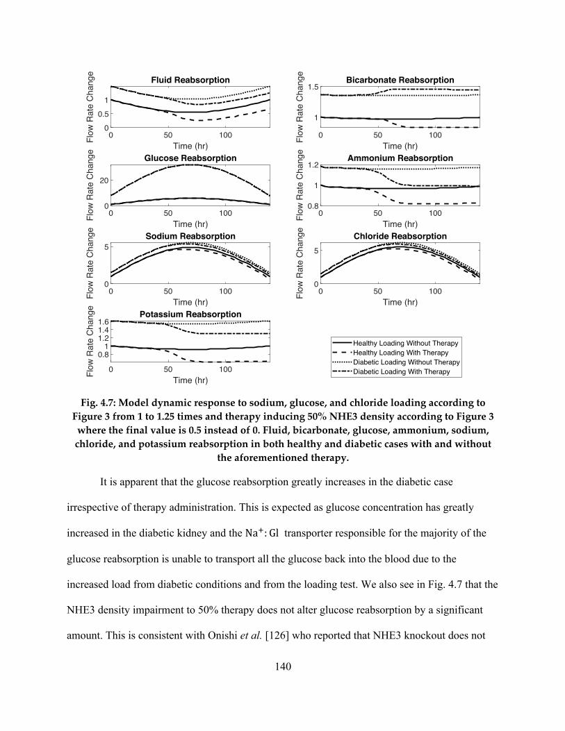
140
Fig. 4.7: Model dynamic response to sodium, glucose, and chloride loading according to Figure 3 from 1 to 1.25 times and therapy inducing 50% NHE3 density according to Figure 3 where the final value is 0.5 instead of 0. Fluid, bicarbonate, glucose, ammonium, sodium, chloride, and potassium reabsorption in both healthy and diabetic cases with and without
the aforementioned therapy.
It is apparent that the glucose reabsorption greatly increases in the diabetic case
irrespective of therapy administration. This is expected as glucose concentration has greatly
increased in the diabetic kidney and the NaF: Gl transporter responsible for the majority of the
glucose reabsorption is unable to transport all the glucose back into the blood due to the
increased load from diabetic conditions and from the loading test. We also see in Fig. 4.7 that the
NHE3 density impairment to 50% therapy does not alter glucose reabsorption by a significant
amount. This is consistent with Onishi et al. [126] who reported that NHE3 knockout does not
0 50 100Time (hr)
00.5
1
Fluid ReabsorptionFl
ow R
ate
Cha
nge
0 50 100Time (hr)
1
1.5Bicarbonate Reabsorption
Flow
Rat
e C
hang
e
0 50 100Time (hr)
0
20
Glucose Reabsorption
Flow
Rat
e C
hang
e
0 50 100Time (hr)
0.8
1
1.2Ammonium Reabsorption
Flow
Rat
e C
hang
e0 50 100
Time (hr)
0
5Sodium Reabsorption
Flow
Rat
e C
hang
e
0 50 100Time (hr)
0
5
Chloride Reabsorption
Flow
Rat
e C
hang
e
0 50 100Time (hr)
0.81
1.21.41.6
Potassium Reabsorption
Flow
Rat
e C
hang
e
Healthy Loading Without TherapyHealthy Loading With TherapyDiabetic Loading Without TherapyDiabetic Loading With Therapy

141
attenuate hyperglycemia associated with diabetes. The NHE3 therapy has a large effect on the
ammonium reabsorption in the diabetic kidney, bringing it closer to healthy levels.
Importantly, fluid, potassium, and ammonium reabsorption for the diabetic kidney with
therapy administered moves the reabsorption of all solutes more closely in line with that of a
healthy kidney. This is an important effect of the therapy where fluid retention that typically
occurs in the case of the diabetic kidney is reduced. For bicarbonate reabsorption, this increased
reabsorption can disrupt blood pH levels in the case of the diabetic kidney. Bicarbonate is an
essential solute for maintaining this pH balance in the kidneys. The pH balance in the kidneys
can have adverse whole body consequences if disrupted [1]. We observe in Fig. 4.7 that the
NHE3 therapy does in fact increase bicarbonate reabsorption to levels further beyond those of a
diabetic kidney during this loading.
Sodium and chloride reabsorption are largely unaffected by the NHE3 therapy, Fig. 4.7,
administered presumably due to the high loading of both solutes. Though we do note that the
NHE3 therapy in both cases moves reabsorption of both solutes closer to the values seen in the
healthy kidney during loading.
Taking into account aforementioned results, fluid, potassium, glucose, ammonium,
sodium, and chloride reabsorption are positively affected by NHE3 expression reduction to 50%
density in the case of salt and sugar loading. Certain diabetic therapies such as insulin, according
to Packer [85], can lead to an increase in NHE3 expression. This increased expression can have
adverse effects on all reabsorptions aforementioned, namely fluid retention that is associated
with insulin therapy.

142
4.3.4 Stability Analysis
In order to check if the pencil (E, I), is regular, it suffices to show the existence of one K
such that det(KE − I) ≠ 0. For our system we arbitrary found K = 5 × 10&"G from an
exhaustive search, to make det(KE − I) ≠ 0. For this value, the determinant of the pencil is
−2.4 × 10"1 and hence the pencil is regular.
We next looked at the eigenvalues of the pencil, from (4.37), for the linearized version of
the model. We have 70 eigenvalues. Considering just the real parts of these finite eigenvalues, 64
are negative and 6 are zero. This implies that the system is marginally stable based on the
solution to the differential equation including sinusoidal components [13]. Further, it implies that
a bounded input will necessarily produce a bounded output within a given region of oscillation.
This is important because it implies that the proximal tubule reabsorption will not be life-
threatening during changes to inputs from the glomerulus, within a neighborhood around the
equilibrium point, as is true in real life since the proximal tubule reabsorptions returns to
equilibrium with many perturbations throughout the day.
In a paper by Weinstein and Sontag [101], the authors note that in healthy kidney
function, there are routinely swings in proximal tubule fluid flow and proportional changes in
sodium reabsorption. This is known as the glomerulotubular balance and it was investigated in
[101], how transporter regulation may account for this balance and subsequent stability of the
system. It was determined in [101] that transporter parameter modulation is a function of cell
volume, electrical potential, and interspace pressure acts to stabilize cell volume, sodium flux,
and cell pH. The proposed feedback via transporter modulation in [101] is left as a hypothesis to
by the authors be tested in experiments.

143
In the presence of known autoregulation mechanisms in the kidney, such as the myogenic
response, the tubuloglomerular feedback, and the renin-angiotensin mechanism, fluid flow into
the proximal tubule is contained within a tight range. In [101], it is suggested that there is an
intrinsic autoregulation within the proximal tubule. Therefore, it is not expected for the proximal
tubule to be asymptotically stable to all bounded inputs since these autoregulation systems are
required for a healthy kidney.
4.4 Conclusion
In this chapter, we developed a mathematical model that captures the transport dynamics
of the proximal tubule, the most active portion of the nephron. We have developed a novel
modular mathematical dynamic model based on physiological first principles that was subjected
to different validation steps. We first replicated trends and steady-state results from experiments
and other models in the literature and found our model to be in good standing. Further, we have
investigated the effects of sodium-hydrogen transporter (NHE3) therapy in the case of healthy
and diabetic kidneys. We see in our simulation results that a reduction of NHE3 expression to
50% both in baseline input and loading of salt and glucose cases, partially restores diabetic
kidney fluid, sodium, ammonium, potassium, and chloride reabsorption to values that coincide
with a healthy kidney under identical conditions. This model can be a tool for testing NHE3
therapy on a population of diabetic patients, or on an individual diabetic patient, after
personalization.
Again, the goal of NHE3 therapy for a diabetic kidney is to reduce hyper-reabsorption
and subsequently glomerular hyperfiltration that can lead to diabetic nephropathy. With reduced
sodium and chloride reabsorption from NHE3 suppression, the tubuloglomerular feedback
mechanism will not be activated increasing glomerular filtration rate, leading to hyperfiltration.

144
Therefore, in terms of reducing hyperfiltration, the NHE3 effects demonstrated by the model,
reduce sodium and chloride reabsorption in the proximal tubule thereby preventing
hyperfiltration.
The model, a differential-algebraic set of equations (DAEs), was linearized and the
stability around the equilibrium point was analyzed, showing marginal stability. Solving a
complex DAE is similar to solving a stiff system and the complexities of solving this system
were also discussed.
The model presented was developed using a first principles approach based on renal
physiology. It improves upon the current literature of proximal tubule models in its development
strategy, dynamic simulation, inclusion of 17 solutes, and removal of assumptions about solute
transport and pressure-volume constraints. This model, after validation, can be used to
understand kidney diseases. We can simulate the time-varying response of the proximal tubule to
therapy and capture the dynamics of diseases, as demonstrated in our clinical scenario
simulations. Many other disease and intervention scenarios can be similarly simulated.

145
Chapter 5: Rat Proximal Tubule Model - Parameter Estimation &
Disease Classification
5.1 Introduction
A physiological model of a complex system allows for the understanding of variables and
parameters most of which are unobservable. Variables are states of the system, like pressure,
concentration, and flow. Parameters characterize physical properties of a system and typically
appear as coefficients of the variables in system’s equations; they are a window into system
health. In the proximal tubule of the kidney there are several vital transporters that determine
overall kidney health. We make use of the previously validated lumped, ordinary differential
equation model from the previous chapter, of the nephron proximal tubule model with
parameters that describe these vital transporters. In the current chapter, we focus on the
NaF: HCO2& (sodium-bicarbonate), KF: Cl& (potassium-chloride), NaF: HF (sodium-hydrogen),
and Cl&: HCO2& (chloride-bicarbonate) co-transporters in an effort to determine their expression
(density). These transporters are important because the largest flow rates of sodium, bicarbonate,
chloride, and potassium occur across these co-transporters as compared with any others in the
proximal tubule [90]. Therefore, alterations in the expressions of these co-transporters will
greatly affect kidney function.
Parameter estimation is the process of using measured input and output variables in order
to compute the parameters. Estimating parameters is important for determining diseases, where
altered parameters are indicative of the state of the system. The process can also be used to
personalize a model to a specific patient. A personalized model can then be used to test therapy
scenarios on the model rather than the patient. Bayesian estimation is an approach to accomplish

146
parameter estimation. It leverages prior information in the estimation to improve the confidence
of each estimation. This technique is well suited for clinical applications, where patient
demographic and comorbidity information are readily available and can be incorporated into the
prior information for a Bayesian estimation. As described by Spielgelhalter [128] a Bayesian
approach is best for providing additional tools for disease classification where the prior
prevalence (probability) of such disease is known. Considering the patient population as
stochastic, with a Gaussian distribution, it makes sense to use this type of probabilistic approach
for disease classification. With a vast majority of patient medical records being stored and
aggregated, there is an abundance of prior information for different patient populations. Because
of this, any estimation technique that can make use of this information lends itself nicely to the
cause. Several papers have utilized parameter estimation techniques for the kidneys and
specifically the proximal tubule [43]–[47] via least-squares or nonlinear least-squares. These
papers were focused on either estimating resistances, capacitances, or transporter parameters for
kinetic models of a single co-transporter. Estimations were carried out with healthy data,
spontaneously hypertensive data, or data after glucose loading in rats. Our goal is to study which
model outputs are needed as estimation inputs in order to achieve high accuracy estimation of
parameters of the four aforementioned co-transporters. We analyze how proximal tubule
variables, such as the pressure, electric potential, or concentrations of sodium, potassium,
chloride, glucose, urea, and bicarbonate, are affected when several co-transporter densities are
changed simultaneously.
Using Bayesian estimation, we are able to estimate these transporter densities using
measurable model outputs including the aforementioned pressure, electric potential, and solute
concentrations. We are also able to thereby observe unmeasurable model outputs such as

147
pressures and concentrations in the epithelial cells and interspaces corresponding to the perturbed
transporter density via simulation. The estimation results are validated using data that was
collected from rats with normal, decreased, and increased NaF: HF transporter expressions.
Using the measured bicarbonate concentration and pH levels from the experiments, we estimate
the parameters of all four co-transporters for all cases of NaF: HF expression and report the
difference between the estimated and the true values. Further, we evaluate estimation results by
comparing fluid, sodium, bicarbonate, and glucose reabsorption from model outputs using the
true parameter density (as measured) and model outputs using estimated parameter densities. To
study variable response to changes in transporter density, we begin by conducting a sensitivity
analysis that can also identify suitable inputs for the Bayesian estimation. Using the inputs
highlighted from the sensitivity analysis, we then conduct several estimations, with model-
generated noisy data, for different transporter expressions. We again evaluate the performance of
the estimation by comparing reabsorption flow rates of those corresponding to true parameters
and those corresponding to estimated parameters. High accuracy was determined by minimal
error between parameter estimations as compared to true co-transporter parameter expression
and minimal error between estimation derived reabsorption flow rates compared to true
reabsorption flow rates.
5.2 Methods
5.2.1 Model Structure
In the model, we divide the proximal tubule, based on physiological transport differences,
into two sections: the proximal convoluted tubule (PCT) and the proximal straight tubule (PST).
Similar to Christensen et al. [105], we consider the PCT to be the first 70% (0.7 cm) of the
proximal tubule in length and the PST to be the last 30% (0.3 cm). Each section is further

148
tessellated into three nodes: tubule, epithelial cell (EC), and interspace between the cells (IS). The
source to the system (where filtrate enters the proximal tubule) is Bowman’s space (BS) and the
sinks are the interstitial fluid (IF) and the descending limb of Henle (LDN). Flow throughout the
system is shown in Fig. 4.1, where arrow directions indicate positive flow.
At an arbitrary node m, the time-varying variables we consider are hydraulic pressure,
nH(/), in mmHg, concentration, [H(/), in mmol/mL, and electric potential, =H(/), in mV.
Between arbitrary nodes m and o, the flow of fluid and solutes is given by pH&I(/), in mL/s,
and UH&I(/), in mmol/s, respectively. Volume at any node is given by integrating the fluid flow,
qH(/) = ∫ pH(/)s/ in mL, where pH is the net flow into node m. Similarly, mass at any node is
given by integrating the solute flow, 8H(/) = ∫ UH(/)s/ in mmol, where UH is the net solute flow
into node m. The solutes included in the model are those that are also included in [90]: NaF, KF,
Cl&, glucose (Gl), urea (Ur), an impermeant protein (Imp&) with valence z = −1, HCO2&, H1CO2,
CO1, HPOJ1&, H1POJ&, NH2, NHJF, HF, HCO1&, H1CO1, an impermeant buffer (Buff&) with
valence z = −1, and a protonated impermeant buffer (HBuff) with valence z = 0. These solutes
are included because they comprise the solute constituents of the co-transporters and associated
buffer pair solutes. The full set of equations is comprised of those previously derived in (4.1) –
(4.27).
5.2.2 References & Parameters
Concentrations from a Ringer’s solution (an isotonic solution relative to interstitial fluid)
were used as the source and sink values at BS, IF!, and IF". For the LDN node, concentrations
were set to concentrations in the PST, plus the difference between the values at the PCT and PST
divided by the ratio of their lengths. We use the lengths instead of the volumes since the cross-
sectional areas are identical. Since these solutes are all reabsorbed in greater amounts than

149
secreted back into the nephron, this is a fair assumption that concentrations would decrease in the
LDN. Reference pressure and voltage values needed at BS, IF! and IF", and LDN nodes were
from [90]. Reference volumes are not needed for sources or sinks, as they do not appear in any
equation.
The parameters for axial fluid flow were calculated using the Hagen-Poiseuille relation,
from the Navier-Stokes equations, assuming a constant radius of the tubule and laminar flow:
%H&I( =8|HI~�ÄHIJ
, (5.1)
where |HI is the average length between nodes, ÄHI is the average radius between nodes, and ~ is
the blood viscosity, assumed to be 6.4´10-6 mmHg⋅s. Inlet flow from BS was set to 35 nL/min
and solute flow from BS to PCT was restricted to only advective flow since the diffusive flow
here is negligible.
For axial solute flow, all reflection coefficients were set to 0 since there are no
membranes to impede the flow of these solutes axially. For the diffusive resistance along the
tubule, diffusion coefficient values in an aqueous, well stirred water solution were found from
[110] and [111] and then adapted to our system by multiplying by the cross-sectional area of the
tubule and dividing by the length:
%H&I, =%Å,Ç�ÄHI1
|HI, (5.2)
where %Å, is the diffusion coefficient and Ç is the temperature adjustment factor for the solutes
(in this case, the adjustment for 37℃ is Ç = 1.339) used to account for change in the diffusion
coefficient based on temperature.
All remaining parameters were adapted from [90] to fit a lumped model with our model units. A
complete list of all parameters can be found in Table 4.1 with the co-transporter parameters for
NaF: HCO2&, KF: Cl&, NaF: HF, and Cl&: HCO2& reproduced in Table 5.1.

150
Table 5.1: Co-transporter permeabilities [mmol2/J/s] and stoichiometric ratios.
from to ÑÖ&: XÑÜK& áàF: XF âF: ÑÖ& áàF: XÑÜK
& äÑã åÑ?=@ 7.92×10⁻¹⁰ 1.09×10⁻⁹ 0 0 åÑ?=@ çé?=@ 0 0 1.98×10⁻⁹ 1.98×10⁻⁹ åÑ?=@ çèL 0 0 5.50×10⁻¹¹ 5.5×10⁻¹¹ äéã åÑ?M@ 3.39×10⁻¹⁰ 4.67×10⁻¹⁰ 0 0 åÑ?M@ çé?M@ 0 0 8.48×10⁻¹⁰ 8.48×10⁻¹⁰ åÑ?M@ çèN 0 0 2.36×10⁻¹¹ 2.36×10⁻¹¹
Ratios 1:-1 1:-1 1:1 1:3
5.2.3 Bayesian Estimation
Since we have developed the rat proximal tubule model using a first-principal approach,
the parameter values have physical meaning, such as transporter expression or hydraulic
resistance of tubules. Bayesian estimation is a parameter estimation technique that uses prior (a-
priori) knowledge of parameter values in order to better estimate (or predict) these parameters
[16]. Typically, medicine is evidenced-based, where physicians integrate: clinical experience,
patient values, and the best available research information [129]. Using Bayesian estimation for
parameter estimation in our application essentially comprises all parts of this definition for
evidence-based medicine: clinical experience (prior prevalence and population information),
patient values (input and output signals), and the best available research information (the
mechanistic model). By utilizing all three of these components we are able to accurately estimate
patient parameter values and subsequent diseases.
The process of this parameter estimation consists of finding a probability distribution of
each parameter to be estimated given the values of input and output variables. We can then use a
maximum-a-posteriori (MAP) estimator to select the parameter values that have the highest
probability as the final estimated parameter value for all parameters estimated. Another
advantage to this approach is when using the estimated parameters for disease classification

151
based on parameter values. Essentially, we are also estimating a confidence via a distribution for
each estimate and hence a confidence that a particular patient has a particular disease.
We are specifically interested in estimating scaling values multiplying the result of (4.10)
for the NaF: HCO2&, KF: Cl&, NaF: HF, and Cl&: HCO2& co-transporters. These transporters are
important because the largest flow rates of sodium, bicarbonate, chloride, and potassium occur
across these co-transporters as compared with any others in the proximal tubule [90]. These
scaling values represent the density/expression of each co-transporter. A value less than one
represents an under-expressed transporter, while a value of one represents a healthy transporter,
and a value greater than one represents an over-expressed transporter. An over-expressed or
under-expressed transporter can lead to a decrease or increase in solute reabsorptions throughout
the proximal tubule that can result in solute concentrations that are dangerously low or high. The
4 × 1 vector of scaling (density) parameters of the NaF: HCO2&, KF: Cl&, NaF: HF, and Cl&: HCO2&
co-transporters that we aim to estimate is ê. Here, we are assuming that every parameter is
stochastic and varies between a range of 0 to 2. Again, this approach makes sense because
patient parameter values are typically stochastic and normally distributed across the population.
Our prior information about these parameters will be derived from population statistics. The
ë × í matrix of model outputs in time is given by
ì(/) = î(/, ê), (5.3)
where ë is the number of measurements at time /, í is the number of outputs, and î is the model
of the system. The collected measurements will inevitably be corrupted by noise and since the
model cannot perfectly describe the physics, we introduce the ë × í matrix of noisy
measurement outputs,
ï(/) = î(/, ê) +ñ, (5.4)

152
where ñ is a matrix of white Gaussian noise on each model output (estimation input). The
estimation is used to obtain a value of ê, êó, from the available measurements, ï. This is done by
first applying Bayes’ theorem, given by
9(ê|ï) =9(ï|ê) ⋅ 9(ê)
9(ï), (5.5)
where 9(ê|ï) is the conditional (a-posteriori) probability of ê values given the available
measurements ï, 9(ï|ê) is the joint conditional probability of ï, given ê values, 9(ê) is the
combined (product) a-priori probability density function (pdf) of each parameter, and 9(ï) is the
joint pdf of the measurements. We are interested in solving for 9(ê|ï) which will inform us of
the probability of the patient having certain parameter values given the patient measurements.
The 9(ï|ê) term is the likelihood function, and a measure of the probability of achieving patient
measurements given a set of parameter values. When evaluating 9(ê), we make use of the prior
information known about the population and parameter values. Finally, the term 9(ï), having no
functional dependence on ê, is not strictly necessary for evaluating (5.5), but instead used to
scale the results based on the probability of achieving the given measurement values.
The MAP estimation for a single ô is defined as
ôöOP# = argmaxQ9(ô|ù). (5.6)
For multiple parameters, ê is a vector, and the MAP estimated parameter vector value êó for each
is defined as the argmax of the marginalization of 9(ê|ï) for each a-posteriori pdf. The
marginalization is defined as the sum over all possible values of the parameters, more
specifically, the multiple summations over every other parameter other than the specific element
of ê. For the ;th element of êó, this is discretely defined by
ôö6OP# = argmaxQ+
ûüûüû9(ê|ï)R
⋅ ΔôR° ⋅S
ΔôS° ⋅ ΔôTT
, (5.7)

153
where ΔôR is the discrete distance between neighboring possible values for ôR (and similarly for
ôS and ôT). The a-priori pdfs for each of the four transport scaling parameters were chosen as
normal distributions with a mean of 1 and standard deviation of 0.2. This value of standard
deviation was chosen since it is half the value of what is determined to be a diseased transporter
in [125]. In practice, these values may be different depending on prior patient knowledge. Some
prior patient knowledge includes patient demographics and information about other
comorbidities.
The conditional probability, 9(ï|ê), is the product of conditional probabilities, 9(¢|ê),
for each estimation input, where ¢ is an ë × 1 vector of measurements in time for that input.
Practically speaking, 9(¢|ê) is a matrix evaluated for all combination of allowable, ê, defined as
ê = ê£ values, as dictated by the domain of 9(ê). One element of the conditional probability,
9§¢•ê = ꣶ, for a given value of ê = ê£ and one estimation input signal is defined as
9§¢•ê = ꣶ =exp ß−12 (¢ − ®)
U ⋅ ©V&" ⋅ (¢ − ®)™
´(2�)W|©V|, (5.8)
where ©V = ¨I1 ⋅ ≠ is the covariance matrix of the measurement noise with standard deviation
¨I, |©V| is the determinant of the covariance matrix, and ® is a vector of the estimation inputs
calculated from the model given ê = ê£. We define a matrix Æ comprising model outputs, in
time, for all discrete combinations of ê values allowable. From Æ, for a given ê£, we select the
vector of estimation inputs ®, corresponding to ê£. For example, for a four element ê vector, with
10 possible values for each element, Æ will be a 5-dimensional matrix with 10 elements along the
first four dimensions and ë along the last. In selecting the ë × 1 vector ®, we select the
elements of Æ, along the first four dimensions corresponding to the value of ê£.The matrix Æ, is
computationally expensive to compute, depending on the resolution of the parameter values used

154
in the calculation. However, this term need only be calculated once, prior to any parameter
estimations. Hence, evaluating 9(¢|ê), for a specific patient, is a simple substitution of ¢ values
prior to the parameter estimation using Bayesian theorem in (5.5) and evaluate for all possible
parameter value combinations.
Given that the term 9(ï|ê) ⋅ 9(ê) = 9(ï, ê) is the joint pdf of 9(ï, ê), we can compute
9(ï) as the following
9(ï) = Ø9(ï, ê)Q
sô = Ø9(ï|ê) ⋅ 9(ê)Q
sô. (5.9)
With all three terms in Bayes’ theorem, we can then calculate 9(ê|ï) using (5.5). To find
each component of ê, we can marginalize the pdf 9(ê|ï), as described above, and then calculate
the MAP value for each a-posteriori pdf using (5.6).
5.3 Results & Discussion
We validate the estimation results using data from real rats. We will use the inputs
available from the study as estimation inputs. Next, we conduct a sensitivity analysis to select
which inputs (when available) allow for better estimation. Finally, we generate simulation data
for various diseased states and conduct several estimations to investigate how input signals,
degree of noise, and number of data points per signal provided affect the estimations.
Specifically, we will consider the results in terms of correct parameter estimations as well as
percent error for reabsorption flows (model-predicted variables using the estimated parameters).
5.3.1 Parameter Estimation Validation
In this section, we apply Bayesian estimation to the model to estimate co-transporter
parameters and hence validate the performance of the estimation technique by estimating co-
transporter expressions utilizing rat data collected from experiments. This allows us to discern

155
which co-transporters have altered or unaltered expressions. Further, we analyze how the model
outputs using the estimated parameter values compare to the true model outputs.
Girardi et al. [125] investigated the effect of parathyroid hormones on the expression of
the NaF: HF transporter in the proximal tubule of rats. Rats without altered NaF: HF transporters
were compared to those with decreased and increased NaF: HF transporter densities. After eight
days, bicarbonate concentrations and pH levels were measured and compared to the measured
baselines. A western blot analysis was conducted to determine the expression change of the
NaF: HF transporter. We used our model and estimation technique to determine the expression of
each of the four co-transporters, NaF: HCO2&, KF: Cl&, NaF: HF, and Cl&: HCO2&, and the degree
of disease, namely the new density of the transporters.
The estimation results are shown in Fig. 5.1. All parameter estimations consisted of two
measurements at two time points, an initial healthy value for [#$%X$Y)( and pH#$% and a final value
8 days after disease insult. Fig. 5.1a shows the estimation results for a healthy NaF: HF
transporter, Fig. 5.1b shows the estimation results from rats with impaired NaF: HF transporter
density to 60% of the baseline, and Fig. 5.1c shows the estimation results from rats with a
NaF: HF transporter density 150% of the baseline. Each estimation was conducted 100 times and
the results were averaged.

156
(a)
(b)
0 0.5 1 1.5 2Scaling of Transporter Parameter
0
1
2
Prob
abilit
y of
Sca
ling Na+:HCO-
3 Transporter
PriorPosteriorTrue
0 0.5 1 1.5 2Scaling of Transporter Parameter
0
1
2
Prob
abilit
y of
Sca
ling K+:Cl- Transporter
PriorPosteriorTrue
0 0.5 1 1.5 2Scaling of Transporter Parameter
0
2
4
Prob
abilit
y of
Sca
ling Na+:H+ Transporter
PriorPosteriorTrue
0 0.5 1 1.5 2Scaling of Transporter Parameter
0
1
2
Prob
abilit
y of
Sca
ling Cl-:HCO-
3 Transporter
PriorPosteriorTrue
0 0.5 1 1.5 2Scaling of Transporter Parameter
0
0.5
1
1.5
2
Prob
abilit
y of
Sca
ling
Na+:HCO-3 Transporter
PriorPosteriorTrue
0 0.5 1 1.5 2Scaling of Transporter Parameter
0
0.5
1
1.5
2
Prob
abilit
y of
Sca
ling
K+:Cl- Transporter
PriorPosteriorTrue
0 0.5 1 1.5 2Scaling of Transporter Parameter
0
1
2
3
Prob
abilit
y of
Sca
ling
Na+:H+ Transporter
PriorPosteriorTrue
0 0.5 1 1.5 2Scaling of Transporter Parameter
0
0.5
1
1.5
2
Prob
abilit
y of
Sca
ling
Cl-:HCO-3 Transporter
PriorPosteriorTrue

157
(c)
Fig. 5.1: Bayesian estimation results for three cases of &4%: 6% transporter health. Prior probability density function for each parameter shown in dashed line, true parameter
density shown in blue, and estimation probability shown in solid black line. Maximum a-posteriori estimate is highest point on the a-posteriori probability curve. (a) All transporters healthy. (b) Impaired &4%: 6% transporter to 60% baseline density, with all other transporters
healthy. (c) Overactive &4%: 6% transporter to 150% baseline density, with all other transporters healthy. All data from rats from [125].
In Fig. 5.1a (the healthy case), the estimation’s MAP values, as shown by highest point
on the posterior curve, for each transporter density are correct as compared to the true value
(vertical line). In other words, the estimation MAP values match the true values. Further, the a-
posteriori probability of each transporter density (after estimation) has a higher peak at the
estimated value as compared to the a-priori distribution. This implies that the estimation
likelihood for those parameters’ values is higher with the given measurements.
0 0.5 1 1.5 2Scaling of Transporter Parameter
0
1
2
3
Prob
abilit
y of
Sca
ling
Na+:HCO-3 Transporter
PriorPosteriorTrue
0 0.5 1 1.5 2Scaling of Transporter Parameter
0
0.5
1
1.5
2
Prob
abilit
y of
Sca
ling
K+:Cl- Transporter
PriorPosteriorTrue
0 0.5 1 1.5 2Scaling of Transporter Parameter
0
1
2
3
Prob
abilit
y of
Sca
ling
Na+:H+ Transporter
PriorPosteriorTrue
0 0.5 1 1.5 2Scaling of Transporter Parameter
0
0.5
1
1.5
2
Prob
abilit
y of
Sca
ling
Cl-:HCO-3 Transporter
PriorPosteriorTrue

158
In Fig. 5.1b, for the impaired NaF: HF transporter case, the a-posteriori pdf for the
NaF: HCO2& , KF: Cl&, and Cl&: HCO2& estimates are all within 10% of the true scaling and
indicative of healthy functioning co-transporters. The MAP value for NaF: HF was correctly
estimated to be 60%. Hence, the estimation has correctly identified three transporters as healthy,
and the NaF: HF transporter as diseased. We note that the MAP value for the NaF: HFtransporter
is very near the second most probable value of 70% (as determined by the vertical height). This
means that the estimation has determined that the NaF: HF density is most likely either 60% or
70%. In both cases, the estimation would still have correctly identified the NaF: HF transporter
as diseased, as indicated by estimated transporter density lower than 20% the baseline. This 20%
threshold for declaring a transporter diseased is based on the standard deviation used for the a-
priori pdf curves. In practice, this value may differ and is up to the physician to decide.
In Fig. 5.1c, for the case of increased density, we once again see the NaF: HCO2& ,
KF: Cl&, and Cl&: HCO2& transporters are estimated to be within 10% of the true scaling and
indicative of healthy function co-transporters. The NaF: HF transporter density in the overactive
case has a MAP value of 120%. This 120% value is indicative of a disease. Similarly, to the
impaired case, there are in fact two estimation values with similar likelihood for this transporter,
120% and 110%. The true value was 150% and the estimation has underestimated the NaF: HF
density. However, at the MAP value, the estimation results still imply a diseased NaF: HF
transporter, with all other transporters healthy.
Further, we compared the reabsorption flow model outputs of fluid, sodium, glucose, and
bicarbonate since drastic changes in the reabsorption of these constituents can greatly affect the
health of the kidney [5]. Since the MAP estimation for the healthy case proved to be correct for
all transporter densities in Fig. 5.1a, we correctly observe no error between reabsorption flows

159
since all parameter values are identical to the baseline. For the case of impaired NaF: HF
transporters, using estimated MAP parameters, fluid and sodium reabsorption flows were within
7.5% and 7.1% respectively, of the true reabsorption flows as determined by the true transporter
densities. Glucose reabsorption was within 0.11% of the true value and bicarbonate reabsorption
was within 4.97% of the true value. This indicates that although the estimated (MAP) transporter
density values are slightly different from the true values, the model with estimated parameter
values yields fairly accurate model outputs as compared to the true system outputs. For increased
expression of NaF: HF transporters, it was calculated that fluid and sodium reabsorption were
within 9.2% and 8.8% respectively, of the true reabsorption, glucose reabsorption was within
0.5%, and bicarbonate reabsorption was within 4.98%. This again indicates that although the
estimated (MAP) transporter density values are different from the true values, all reabsorption
flows of the model using the corresponding parameters are within 10% of the true reabsorption
flow values. These estimations have therefore been shown to be capable of estimating diseased
co-transporter parameters, as well as reabsorption flows within 10% of the true reabsorption
values.
5.3.2 Sensitivity Analysis
Our goal is to understand which variables are likely to change given an alteration in the
co-transporter expression/density. This will allow us to conclude which variables are good
indicators of altered co-transporter expressions. We conducted a sensitivity analysis by
individually varying all four of the transporter density parameters from 0 to 2 times their baseline
values in increments of 0.1 and then recorded the variable value changes with respect to their
baselines. These parameter ranges have real, physical meaning and hence are physiologically
bounded to be positive, though the perturbation range allowed for increases and decreases from

160
baseline. We calculated a Σ value to quantify how sensitive a particular variable, +, is to a
change in a particular parameter, 9, based on the change of both the parameter and variable value
from their baseline values as
Σ = ±Δ+Δ9
⋅9+±. (5.10)
The results of this sensitivity analysis for all variables in the proximal convoluted tubule are in
Fig. 5.2, where the sensitivity values for each variable have been normalized such that the largest
sensitivity is 1 by dividing by the largest sensitivity values to easily compare variable
sensitivities to the parameter changes. For each system variable, there are four bars, representing
the sensitivity value of that variable to each of the four co-transporters. We specifically analyzed
values in the convoluted portion of the tubule instead of the straight portion since these values
are more easily measured. In order for a variable to be a good candidate for use in the estimation,
it should be highly (uniquely) sensitive to one parameter and not another. Consider example
transporters A and B and variables 1 and 2. If variable 1 is highly sensitive to transporters A and
B, then deviations of variable 1 from the baseline do not imply which transporter has changed.
However, if variable 2 is highly sensitive to only transporter A, then a deviation from baseline in
variable 2 is likely due to a change in transporter A, and not transporter B.
In Fig. 5.2 we see that formic acid (H1CO1) concentration is highly sensitive to all
transporter densities, as expected since formic acid is pivotal in maintaining the electrically
neutral environment and alteration of any transporter changes the movement of charged particles,
and hence electroneutrality [130]. This implies that estimation using formic acid measurements
would not be indicative of which transporters are healthy and which are diseased. We expected,
and indeed, sodium concentration shows very low sensitivity in response to changes in
Cl&: HCO2& transporter density and very high sensitivity to changes in NaF: HCO2& and NaF: HF

161
transporter density since a large amount of sodium is transported across both of these
transporters. This indicates that relatively unchanged sodium concentrations in the PCT imply
unchanged NaF: HCO2& and NaF: HF transporters, and possible changes to Cl&: HCO2& transporter
density. Glucose is highly sensitive to the NaF: HCO2& and NaF: HF transporters. Since the
majority of glucose is reabsorbed via co-transport with sodium [5], it follows that glucose would
share sensitivity to the same transporters as sodium. Sensitivity to changes in the Cl&: HCO2&
transporter is relatively low across all variables compared to the other transporters with the
exception of hydrogen phosphate (HPOJ1) concentration. Potassium concentration in, Fig. 5.2,
shows increased sensitivity to the KF: Cl& transporter as opposed to the Cl&: HCO2& transporter,
whereas chloride concentration shows increased sensitivity to the Cl&: HCO2& transporter as
opposed to the KF: Cl& transporter. This can be useful during estimation as changes in either
concentration can imply a change in a given transporter.
Fig. 5.2: Sensitivity (7 = |9:;/9;:| for variable : and parameter ;) plot where each
transporter density parameter was varied from 0 to 2 independently in increments of 0.1 and averaged. A 7 was calculated for all variables in the >?@, for each transporter. The sensitivities were normalized such that the largest sensitivity per variable was 1.
Sens
itivity
() V
alue
for Na+:HCO3-
for K+:Cl-
for Na+:H+
for Cl-:HCO3-

162
5.3.3 Parameter Estimation Analysis
In order to analyze how estimation accuracy and performance change in the presence of
varied number of inputs, number of data points of inputs (resolution), and amount of noise, we
conducted several parameter estimations with varied configurations. Data used for the estimation
was generated by the model with noise superimposed on the signals after generation. We tested
estimations with 2, 10, 21, and 41 data points. Data points were down-sampled evenly in time for
cases with less than the baseline number of data points. For cases of more than 2 data points, the
data captures the dynamic changes in variables during transition from the beginning healthy
values to the final diseased values. For noise, we tested 5%, 10%, and 20% of the signal range.
Finally, we tested 11 different combinations of estimation input signals (Table 5.2) based on
conclusions from the sensitivity analysis. All configurations included sodium and potassium with
the addition of other variables, except for the last configuration, which used pH and bicarbonate
concentrations in the proximal convoluted tubule, to mirror the available inputs from [125].
Table 5.2: Co-transporter parameter estimation input configurations.
Proximal Convoluted Tubule Estimation Inputs for each Configuration NaF, KF NaF, KF, Cl& NaF, KF, Gl NaF, KF, Ur NaF, KF, n NaF, KF, = NaF, KF, HPOJ1& NaF, KF, H1CO1 NaF, KF, HCO2& NaF, KF, pH pH, HCO2&
The results of these estimations, for 5% (low) signal range noise and 21 data points, are
presented in Fig. 5.3. Here we estimated parameter values for all combinations of diseased

163
transporters for all four co-transporters. The error results for all of these combination simulations
were averaged together. Fig. 5.3a shows the density percent error for each co-transporter
averaged over all simulations. Fig. 5.3b shows the reabsorption flow percent error calculated
using the MAP of the estimated co-transporter parameters, averaged over all simulations. Fig.
5.3c shows the averages of Fig. 5.3a and Fig. 5.3b across all four transporters and all four
reabsorption flows, respectively. Unsurprisingly the estimation results for varying data points
and noise (regardless of inputs) demonstrated that more data points and lower noise resulted in
better estimations, with average density percent error increasing by approximately 20% for each
doubling in noise or halving of data points.
(a)
Estimation Configuration
Dens
ity %
Erro
r
Na+:HCO3-
K+:Cl-
Na+:H+
Cl-:HCO3-

164
(b)
(c)
Fig. 5.3: Percentage errors for several estimations: (a) average estimated error in co-transporter density across all estimations, (b) average reabsorption error using estimation co-transporter densities, (c) average co-transporter density error over all co-transporters and all
estimations and average reabsorption error across all reabsorption flows and estimations.
We note from Fig. 5.3a that the highest errors exist when estimating the density of the
Cl&: HCO2& co-transporter. However, where we included chloride as an estimation input, the
density error of Cl&: HCO2& significantly decreased, as expected since chloride is one of the
constituents of this transporter. Error significantly decreased with the addition of voltage, HPOJ1,
Estimation Configuration
Reab
sorp
tion
% E
rror Fluid Reabsorption
Na+ ReabsorptionHCO3
- ReabsorptionGlucose Reabsorption
Estimation Configuration
Den
sity
% E
rror
Rea
bsor
ptio
n %
Erro
r Transporter DensityReabsorption Flow

165
HCO2&, or pH. Adding voltage improves accuracy since bicarbonate is the main anion transported
in the proximal convoluted tubule and hence directly affects the electric potential throughout [5].
According to the sensitivity analysis, HPOJ1 showed the highest sensitivity to changes in
Cl&: HCO2& density and therefore it is logical that including this concentration as an estimation
input would improve estimation performance. The addition of HCO2& as well makes sense, since
it is one of the solutes transported via the Cl&: HCO2& transporter. The other transporters are
estimated with similar percent errors across all estimation configurations, with the exception of
using only pH and HCO2& as estimation inputs. This implies that these estimation inputs do not
provide enough information for the estimation to correctly determine transporter densities, with
the exception of the NaF: HF transporter, as also demonstrated by the validation in 5.3.1.
In Fig. 5.3b we see that glucose reabsorption is more accurate when either Cl&or HCO2&
are included with NaF and KF as estimation inputs, as opposed to without. Reabsorption of
HCO2& is estimated within 1% percent error from the true reabsorption in all estimation cases.
This implies that reabsorption of HCO2& is less sensitive to the parameter changes estimated in
Fig. 5.3a. Fluid and NaF reabsorption errors are similar for all estimation configurations. This
makes sense since fluid and NaF are typically absorbed in equal parts as per the
glomerulotubular balance [5].
From Fig. 5.3c, we note that better average accuracy (across all four co-transporters and
across all four considered reabsorption flows) according to both transporter density error and
reabsorption flow error occurs when including Cl&, urea, pressure, voltage, HPOJ1, or pH.
Accuracy was unchanged by including glucose or H1CO1. Based on the sensitivity analysis and
the high sensitivity H1CO1 shows in response to changes in any transporter parameter, it was in
fact expected that including H1CO1 would not improve estimation accuracy. Using only pH and

166
HCO2& as estimation inputs significantly worsens accuracy of transporter density, as density
percent error for the NaF: HCO2&, KF: Cl&, and Cl&: HCO2& co-transporters were all above 50%.
This implies that estimations using just these two inputs will not necessarily estimate transporter
density correctly but can still aid in determining reabsorption flow with the same accuracy as
using concentrations of NaF and KF only. The best estimation of reabsorption flow included
HCO2& and the best estimation of transporter density included Cl&. Including HPOJ1 in the
estimation greatly improved transporter density determination, particularly for the Cl&: HCO2& co-
transporter, reducing density percent error from over 60% to under 30%. This makes sense given
the sensitivity analysis where HPOJ1 was the only solute with high sensitivity to the Cl&: HCO2&
transporter compared to the other co-transporters.
We further analyzed the estimation accuracy in terms of disease classification via an F1
score, which is a measure of accuracy for classification algorithms. We classify a specific
estimation into one of 16 possible combinations, where each of the four co-transporters is
estimated to be in one of two states, healthy or diseased. The determination of diseased
transporters was made via estimated density less than 0.8 times or greater than 1.2 times baseline,
and healthy otherwise. Based on the estimation performance over several scenarios of all
possible disease outcome combinations for the four independent co-transporters, we construct the
confusion matrix, which is a matrix that presents predicted and true classifications via calculation
of the precision and recall of the estimation, which are the measures of exactness and
completeness of the estimation, respectively. The F1 score is the harmonic mean of precision and
recall and quantifies the model performance in estimation. The F1 score is bound between 0
(worst) and 1 (best) in terms of performance. For our simulation configurations, a plot of the
resulting F1 scores, averaged over all possible scenarios is presented in Fig. 5.4. We can see

167
from the results, much like the accuracy measures according to Fig. 5.3, the best performance of
the estimation includes Cl&, HPOJ1, or HCO2&. This was predicted by the sensitivity analysis
where all three concentrations showed varying sensitivity across each transporter density. We
again note little to no improvement of disease classification with the addition of glucose or
H1CO1. Similarly, from the sensitivity analysis, specifically for H1CO1, it was predicted that this
solute would not help in estimation since its sensitivity to changes in transporter density is
largely the same across all transporters.
Fig. 5.4: F1 scores for each estimation configuration. Scores are averaged over all possible
disease outcomes given four independent transporter densities, where a disease is classified via a deviation by at least 20% from baseline density.
Estimation Configuration
F1 S
core

168
The parameters estimated had already been preselected based on diseases we chose to
study. In practice, an intuition is necessary for narrowing down potential diseased transporters
and hence choosing the subsequent potentially injured parameters to estimate. Further, in the
current estimation, invasive data within the proximal convoluted tubule is needed for estimation.
It is possible to estimate proximal convoluted tubule variable values based on blood tests or urine
samples, however, the model would need to be expanded, or the added assumption that no insults
exist elsewhere in the kidney besides the potentially selected transporter parameters to be
estimated would need to be included.
5.4 Conclusion
We have developed a lumped parameter model of the proximal tubule that has been
validated and used in an analysis of co-transporter density estimation. Focusing on the
NaF: HCO2&, KF: Cl&, NaF: HF, and Cl&: HCO2& co-transporters, we have shown how we apply a
Bayesian estimation approach to estimate transporter density. Transporter density is directly
related to the health of the kidneys since alterations in density can lead to irregular filtration.
The Bayesian estimation approach (which leverages prior knowledge about parameter
values) with our model was validated with real rat data to demonstrate the ability to estimate
parameters corresponding to reabsorption flows within 10% of the true reabsorption flows. We
then sought to investigate how estimation performance changes with varied input configurations,
as determined by correct transporter density and corresponding reabsorption flows of fluid,
sodium, glucose, and bicarbonate. We began with a sensitivity analysis that shed light on
variables that are good candidates for estimation based on their sensitivity to transporter
parameters. Sensitivity analysis showed that sodium and glucose are not very sensitive to

169
changes in Cl&: HCO2& transporter expression but highly sensitive to changes in NaF: HCO2& and
NaF: HF transporter densities.
Via several simulations with different estimation input configurations, we determined
that overall estimation of transporter densities and subsequent reabsorption flows were improved
with the inclusion of chloride or bicarbonate concentrations in addition to sodium and potassium
concentrations. The percent density error of Cl&: HCO2& significantly decreased with the addition
of voltage, HPOJ1, HCO2&, or pH. Formic acid, which demonstrated a more uniform sensitivity to
co-transporter density, alterations also showed no improvement in estimation accuracy when
included as an estimation input. This implies that measurements of formic acid will likely not
improve estimation results.
We have demonstrated, that with preselected co-transporters of interest, a parameter
estimation is possible to determine which of these co-transporters are diseased and which are
healthy. Further, we have determined, for the NaF: HCO2&, KF: Cl&, NaF: HF, and Cl&: HCO2& co-
transporters in the proximal tubule, which variable measurements are needed in order to
successfully distinguish between healthy and diseased. Such an analysis on co-transporter
interaction leads to a better understanding of how the proximal tubule and its subset of nodes
operate. Further, the parameter estimation of co-transporter densities will eventually lead to more
targeted therapy for the diseased kidney.

170
Chapter 6: Summary & Future Research
In this thesis, we have shown how physiological modeling can be used for 1) therapy
testing via personalization and co-transporter therapy for diabetes, 2) disease classification of co-
transporter impairment, and 3) to develop a deeper understanding of renal physiology. The
models developed demonstrate how a deeper understanding of renal physiology can be gleaned
from a first-principle approach to modeling. Further, these models could be of great use to
physicians as a tool to understand physiology, test potential therapies in a safe environment, and
diagnosis and predict kidney diseases based on alterations to parameter values estimated using
patient data. Two novel kidney models were presented, one from a rigorous, dynamic
framework, and the other from a steady-state, whole body approach.
A steady-state human model was developed with the intention of investigating the
relationship between mean arterial blood pressure and glomerular filtration rate (GFR). The
model was validated against real patient data from the MIMIC database, a study involving 10
mildly hypertensive and 10 severely hypertensive patients, and other models in the literature. It
was shown that in severely hypertensive patients, the renal autoregulation and vasculature is
affected. A sensitivity analysis varying these parameters was conducted to observe how GFR and
sodium concentrations in the nephron are affected. We observed an inverse relationship between
vascular resistance and GFR. We also noted a significant change in sodium concentration in the
descending limb of Henle in response to changes of these parameters.
Next, the steady-state human model was used in a parameter estimation case study where,
with prior knowledge of the patient disease, we estimated certain parameters for patients having
glomerulonephritis. After parameter estimation we validated the physiological soundness and
error metrics reported, as well as claimed success in personalizing the model for that given

171
patient. This opens to the door to a model where inputs and/or parameters can be varied, as they
would in a therapy, to determine the optimal GFR and UO necessary to achieve healthy kidney
function.
In the development of the dynamic proximal tubule model, we first validated our model
outputs versus those in the literature. From here, we investigated the effects of sodium-hydrogen
transporter (NHE3) therapy in the case of healthy and diabetic kidneys. We saw that a reduction
of NHE3 expression by 50% both in 1) baseline input and loading of salt and 2) glucose cases,
partially restores fluid, sodium, ammonium, potassium, and chloride reabsorption to values that
coincide with a healthy kidney under identical conditions. This is the first step in validation of
this therapy and one that demonstrates the feasibility, via a model, of reducing hyperfiltration.
Finally, we used this model to investigate disease differentiation via parameter
estimation. Using a Bayesian estimation approach, we first validated the model’s capability to
differentiate between diseased transporters using real rat data. Then, using simulated data and a
sensitivity analysis, we showed that overall estimation of transporter density and subsequent
reabsorption flow was improved with the inclusion of chloride and bicarbonate concentrations in
addition to sodium and chloride concentrations in the proximal tubule.
The work presented here prompts several areas where physiological modeling and
healthcare can be further improved. Specifically, the work in each chapter can be extended in the
following ways:
Chapter 2: The human, steady-state model presented in Chapter 2 can be extended into a
dynamic system by including capacitance values for all hydraulic nodes, and time varying
feedback. This extension would allow for the model to be utilized in experiments that require
time varying data. For instance, detecting the onset of a disease, such as RPGN (rapidly

172
progressing glomerulonephritis) The model in its steady-state formulation can also be extended
to differentiate between juxtamedullary and cortical nephrons. Further, the interplay between
neighboring nephrons can also be modeled.
Chapter 3: The extension to the parameter estimation work done in this chapter include:
estimation of unlabeled data, further validation with different populations, and improvements to
the estimation algorithm developed and implemented. Rather than estimating parameters with
prior knowledge of the patient disease, the model can be used to estimate potentially affected
parameters without knowledge of the patient disease. This poses a more difficult problem since
the parameters likely to change depending on the given disease vary significantly from disease to
disease. Validation with different population sets will highlight needed areas of improvement in
the model and estimation. Further, the estimation technique used, can be improved with increases
to speed and accuracy.
Chapter 4: The model presented in Chapter 4 was a highly detailed, lumped dynamic
proximal tubule model. This model can be used to investigate other potential therapies. Different
diseased states can be replicated with the model, while then implementing therapies. The model
can also be expanded to include the remaining parts of the nephron, the peritubular capillaries
that surround the nephron, renal autoregulation, and nephron-to-nephron interaction developing a
network of nephrons that represents the entire kidney. Acute renal diseases in the ICU would
benefit from such an extension.
Chapter 5: In terms of parameter estimation using the model developed in Chapter 5,
further research can include expansion to other diseases that affect the proximal tubule
transporters. This would include estimations of more than four transporter parameters. The
delicate interplay between transporter parameter values can also be modeled. This interplay is the

173
physiological effect where transporter parameter values can change in the presence of other
damaged or hyperactive transporters.
In general, the kidney models developed in this thesis can also be linked and connected to
other physiological models. For instance, the previously developed heart and lung models
described in [130]–[132], included the kidneys as a single node with a single resistance value.
However, this node can be replaced with the human kidney modeled developed here. This would
require further adjustments though as the kidneys are not an isolated organ only interacting with
other organs via the input/output channels of the vasculature. Instead, the kidneys and lungs, in
particular, maintain a delicate acid/base balance that must be properly represented. Also, the full
effects of the renin-angiotensin mechanism on the body must also be included.
With an ever more accurate model of the human body, the applications are limitless in
healthcare. Such a model can aid in the deeper understanding on human physiology and in the
workflow of physicians. Rather than just providing information on decisions related to one
specific organ, the full model can provide details about the entire body.
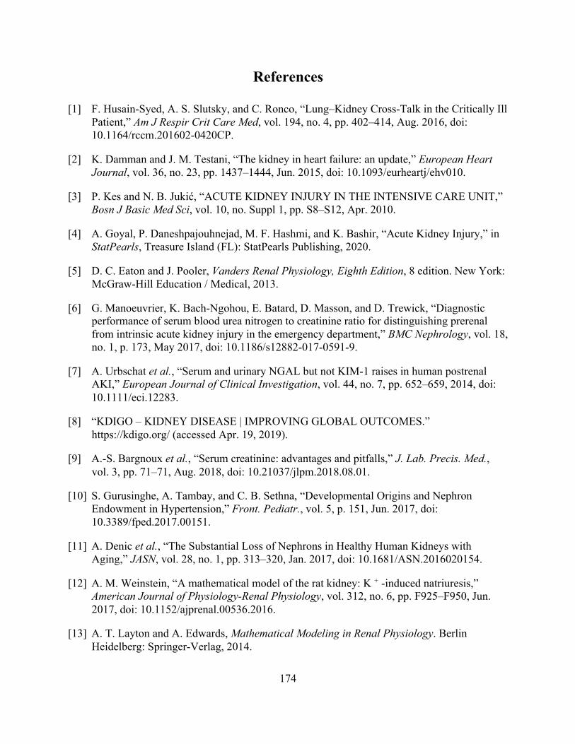
174
References
[1] F. Husain-Syed, A. S. Slutsky, and C. Ronco, “Lung–Kidney Cross-Talk in the Critically Ill Patient,” Am J Respir Crit Care Med, vol. 194, no. 4, pp. 402–414, Aug. 2016, doi: 10.1164/rccm.201602-0420CP.
[2] K. Damman and J. M. Testani, “The kidney in heart failure: an update,” European Heart Journal, vol. 36, no. 23, pp. 1437–1444, Jun. 2015, doi: 10.1093/eurheartj/ehv010.
[3] P. Kes and N. B. Jukić, “ACUTE KIDNEY INJURY IN THE INTENSIVE CARE UNIT,” Bosn J Basic Med Sci, vol. 10, no. Suppl 1, pp. S8–S12, Apr. 2010.
[4] A. Goyal, P. Daneshpajouhnejad, M. F. Hashmi, and K. Bashir, “Acute Kidney Injury,” in StatPearls, Treasure Island (FL): StatPearls Publishing, 2020.
[5] D. C. Eaton and J. Pooler, Vanders Renal Physiology, Eighth Edition, 8 edition. New York: McGraw-Hill Education / Medical, 2013.
[6] G. Manoeuvrier, K. Bach-Ngohou, E. Batard, D. Masson, and D. Trewick, “Diagnostic performance of serum blood urea nitrogen to creatinine ratio for distinguishing prerenal from intrinsic acute kidney injury in the emergency department,” BMC Nephrology, vol. 18, no. 1, p. 173, May 2017, doi: 10.1186/s12882-017-0591-9.
[7] A. Urbschat et al., “Serum and urinary NGAL but not KIM-1 raises in human postrenal AKI,” European Journal of Clinical Investigation, vol. 44, no. 7, pp. 652–659, 2014, doi: 10.1111/eci.12283.
[8] “KDIGO – KIDNEY DISEASE | IMPROVING GLOBAL OUTCOMES.” https://kdigo.org/ (accessed Apr. 19, 2019).
[9] A.-S. Bargnoux et al., “Serum creatinine: advantages and pitfalls,” J. Lab. Precis. Med., vol. 3, pp. 71–71, Aug. 2018, doi: 10.21037/jlpm.2018.08.01.
[10] S. Gurusinghe, A. Tambay, and C. B. Sethna, “Developmental Origins and Nephron Endowment in Hypertension,” Front. Pediatr., vol. 5, p. 151, Jun. 2017, doi: 10.3389/fped.2017.00151.
[11] A. Denic et al., “The Substantial Loss of Nephrons in Healthy Human Kidneys with Aging,” JASN, vol. 28, no. 1, pp. 313–320, Jan. 2017, doi: 10.1681/ASN.2016020154.
[12] A. M. Weinstein, “A mathematical model of the rat kidney: K + -induced natriuresis,” American Journal of Physiology-Renal Physiology, vol. 312, no. 6, pp. F925–F950, Jun. 2017, doi: 10.1152/ajprenal.00536.2016.
[13] A. T. Layton and A. Edwards, Mathematical Modeling in Renal Physiology. Berlin Heidelberg: Springer-Verlag, 2014.
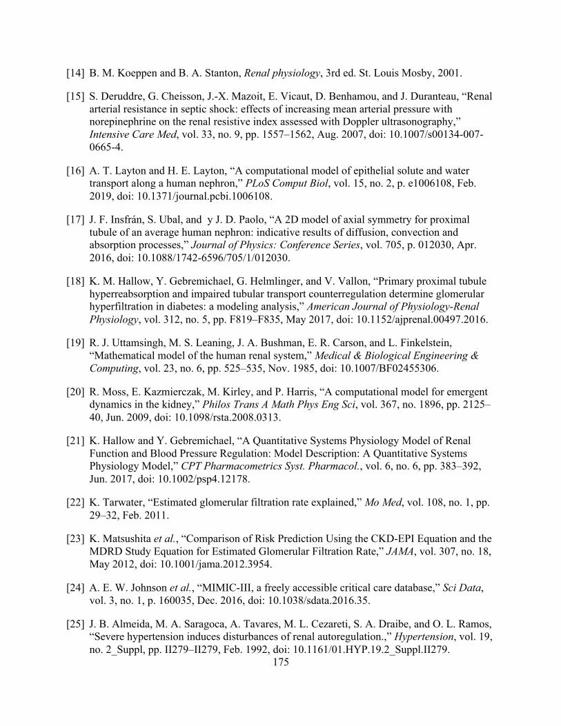
175
[14] B. M. Koeppen and B. A. Stanton, Renal physiology, 3rd ed. St. Louis Mosby, 2001.
[15] S. Deruddre, G. Cheisson, J.-X. Mazoit, E. Vicaut, D. Benhamou, and J. Duranteau, “Renal arterial resistance in septic shock: effects of increasing mean arterial pressure with norepinephrine on the renal resistive index assessed with Doppler ultrasonography,” Intensive Care Med, vol. 33, no. 9, pp. 1557–1562, Aug. 2007, doi: 10.1007/s00134-007-0665-4.
[16] A. T. Layton and H. E. Layton, “A computational model of epithelial solute and water transport along a human nephron,” PLoS Comput Biol, vol. 15, no. 2, p. e1006108, Feb. 2019, doi: 10.1371/journal.pcbi.1006108.
[17] J. F. Insfrán, S. Ubal, and y J. D. Paolo, “A 2D model of axial symmetry for proximal tubule of an average human nephron: indicative results of diffusion, convection and absorption processes,” Journal of Physics: Conference Series, vol. 705, p. 012030, Apr. 2016, doi: 10.1088/1742-6596/705/1/012030.
[18] K. M. Hallow, Y. Gebremichael, G. Helmlinger, and V. Vallon, “Primary proximal tubule hyperreabsorption and impaired tubular transport counterregulation determine glomerular hyperfiltration in diabetes: a modeling analysis,” American Journal of Physiology-Renal Physiology, vol. 312, no. 5, pp. F819–F835, May 2017, doi: 10.1152/ajprenal.00497.2016.
[19] R. J. Uttamsingh, M. S. Leaning, J. A. Bushman, E. R. Carson, and L. Finkelstein, “Mathematical model of the human renal system,” Medical & Biological Engineering & Computing, vol. 23, no. 6, pp. 525–535, Nov. 1985, doi: 10.1007/BF02455306.
[20] R. Moss, E. Kazmierczak, M. Kirley, and P. Harris, “A computational model for emergent dynamics in the kidney,” Philos Trans A Math Phys Eng Sci, vol. 367, no. 1896, pp. 2125–40, Jun. 2009, doi: 10.1098/rsta.2008.0313.
[21] K. Hallow and Y. Gebremichael, “A Quantitative Systems Physiology Model of Renal Function and Blood Pressure Regulation: Model Description: A Quantitative Systems Physiology Model,” CPT Pharmacometrics Syst. Pharmacol., vol. 6, no. 6, pp. 383–392, Jun. 2017, doi: 10.1002/psp4.12178.
[22] K. Tarwater, “Estimated glomerular filtration rate explained,” Mo Med, vol. 108, no. 1, pp. 29–32, Feb. 2011.
[23] K. Matsushita et al., “Comparison of Risk Prediction Using the CKD-EPI Equation and the MDRD Study Equation for Estimated Glomerular Filtration Rate,” JAMA, vol. 307, no. 18, May 2012, doi: 10.1001/jama.2012.3954.
[24] A. E. W. Johnson et al., “MIMIC-III, a freely accessible critical care database,” Sci Data, vol. 3, no. 1, p. 160035, Dec. 2016, doi: 10.1038/sdata.2016.35.
[25] J. B. Almeida, M. A. Saragoca, A. Tavares, M. L. Cezareti, S. A. Draibe, and O. L. Ramos, “Severe hypertension induces disturbances of renal autoregulation.,” Hypertension, vol. 19, no. 2_Suppl, pp. II279–II279, Feb. 1992, doi: 10.1161/01.HYP.19.2_Suppl.II279.

176
[26] D. Rowell and D. N. Wormley, System Dynamics: An Introduction, 1 edition. Upper Saddle River, NJ: Pearson, 1996.
[27] E. N. Marieb and K. Hoehn, Human anatomy & physiology, Eleventh edition. Hoboken, New Jersey: Pearson, 2018.
[28] I. Sgouralis and A. T. Layton, “Mathematical modeling of renal hemodynamics in physiology and pathophysiology,” Mathematical Biosciences, vol. 264, pp. 8–20, Jun. 2015, doi: 10.1016/j.mbs.2015.02.016.
[29] H. Lamport, “Formulae for Afferent and Efferent Arteriolar Resistance in the Human Kidney: An Application to the Effects of Spinal Anesthesia,” J. Clin. Invest., vol. 20, no. 5, pp. 535–544, Sep. 1941, doi: 10.1172/JCI101246.
[30] V. G. Puelles, W. E. Hoy, M. D. Hughson, B. Diouf, R. N. Douglas-Denton, and J. F. Bertram, “Glomerular number and size variability and risk for kidney disease:,” Current Opinion in Nephrology and Hypertension, vol. 20, no. 1, pp. 7–15, Jan. 2011, doi: 10.1097/MNH.0b013e3283410a7d.
[31] S. A. Carter and G. W. Ritchie, “Measurement of Renal Artery Pressures by Catheterization in Patients with and without Renal Artery Stenosis,” Circulation, vol. 33, no. 3, pp. 443–449, Mar. 1966, doi: 10.1161/01.CIR.33.3.443.
[32] L. C. Moore, A. Rich, and D. Casellas, “Ascending Myogenic Autoregulation: Interactions Between Tubuloglomerular Feedback and Myogenic Mechanisms,” p. 20.
[33] R. Moss and S. R. Thomas, “Hormonal regulation of salt and water excretion: a mathematical model of whole kidney function and pressure natriuresis,” American Journal of Physiology-Renal Physiology, vol. 306, no. 2, pp. F224–F248, Jan. 2014, doi: 10.1152/ajprenal.00089.2013.
[34] A. S. Levey et al., “Using Standardized Serum Creatinine Values in the Modification of Diet in Renal Disease Study Equation for Estimating Glomerular Filtration Rate,” Ann Intern Med, vol. 145, no. 4, p. 247, Aug. 2006, doi: 10.7326/0003-4819-145-4-200608150-00004.
[35] A. Remuzzi, S. Puntorieri, A. Mazzoleni, and G. Remuzzi, “Sex related differences in glomerular ultrafiltration and proteinuria in Munich-Wistar rats,” Kidney International, vol. 34, no. 4, pp. 481–486, Oct. 1988, doi: 10.1038/ki.1988.206.
[36] S. R. Monu, H. Wang, and P. Ortiz, “Abstract P1115: Decreased Tubuloglomerular Feedback (TGF) Response in High-Fat Diet Induced Obesity,” Hypertension, vol. 74, no. Suppl_1, Sep. 2019, doi: 10.1161/hyp.74.suppl_1.P1115.
[37] J. Hall, L. Juncos, Z. Wang, M. Hall, J. do Carmo, and A. da Silva, “Obesity, hypertension, and chronic kidney disease,” IJNRD, p. 75, Feb. 2014, doi: 10.2147/IJNRD.S39739.

177
[38] V. Kumar, A. K. Abbas, J. C. Aster, and J. A. Perkins, Eds., Robbins basic pathology, Tenth edition. Philadelphia, Pennsylvania: Elsevier, 2018.
[39] C. Delong and S. Sharma, “Physiology, Peripheral Vascular Resistance,” in StatPearls, Treasure Island (FL): StatPearls Publishing, 2020.
[40] K. Vääräniemi et al., “Lower Glomerular Filtration Rate Is Associated With Higher Systemic Vascular Resistance in Patients Without Prevalent Kidney Disease,” J Clin Hypertens, vol. 16, no. 10, pp. 722–728, Oct. 2014, doi: 10.1111/jch.12405.
[41] “Section 2: AKI Definition,” Kidney International Supplements, vol. 2, no. 1, pp. 19–36, Mar. 2012, doi: 10.1038/kisup.2011.32.
[42] S. Ditlevsen, K.-P. Yip, and N.-H. Holstein-Rathlou, “Parameter estimation in a stochastic model of the tubuloglomerular feedback mechanism in a rat nephron,” Mathematical Biosciences, vol. 194, no. 1, pp. 49–69, Mar. 2005, doi: 10.1016/j.mbs.2004.12.007.
[43] M. Marcano, H.-M. Yang, A. Nieves-González, C. Clausen, and L. C. Moore, “Parameter estimation for mathematical models of NKCC2 cotransporter isoforms,” American Journal of Physiology-Renal Physiology, vol. 296, no. 2, pp. F369–F381, Feb. 2009, doi: 10.1152/ajprenal.00096.2008.
[44] M. Nadal-Quirós, L. C. Moore, and M. Marcano, “Parameter estimation for mathematical models of a nongastric H + (Na + )-K + (NH 4 + )-ATPase,” American Journal of Physiology-Renal Physiology, vol. 309, no. 5, pp. F434–F446, Sep. 2015, doi: 10.1152/ajprenal.00539.2014.
[45] M. J. Lazzara and W. M. Deen, “Model of albumin reabsorption in the proximal tubule,” American Journal of Physiology-Renal Physiology, vol. 292, no. 1, pp. F430–F439, Jan. 2007, doi: 10.1152/ajprenal.00010.2006.
[46] L. D. Parks and D. W. Barfuss, “Transepithelial transport and metabolism of glycine in S1, S2, and S3 cell types of the rabbit proximal tubule,” American Journal of Physiology-Renal Physiology, vol. 283, no. 6, pp. F1208–F1215, Dec. 2002, doi: 10.1152/ajprenal.00021.2002.
[47] A. Folch-Fortuny, F. Arteaga, and A. Ferrer, “Missing Data Imputation Toolbox for MATLAB,” Chemometrics and Intelligent Laboratory Systems, vol. 154, pp. 93–100, May 2016, doi: 10.1016/j.chemolab.2016.03.019.
[48] C. John, E. J. Ekpenyong, and C. C. Nworu, “Imputation of Missing Values in Economic and Financial Time Series Data Using Five Principal Component Analysis (PCA) Approaches,” CBN-JAS, no. Vol. 10 No. 1, pp. 51–73, Aug. 2019, doi: 10.33429/Cjas.10119.3/6.
[49] B. Czarkowska-Pączek, K. Mucha, and L. Pączek, “Age-Related Decline in Renal Blood Flow Could Be a Beneficial and Compensatory Mechanism,” Med Sci Monit, vol. 26, Jan. 2020, doi: 10.12659/MSM.918643.

178
[50] K. Hoang et al., “Determinants of glomerular hypofiltration in aging humans,” Kidney International, vol. 64, no. 4, pp. 1417–1424, Oct. 2003, doi: 10.1046/j.1523-1755.2003.00207.x.
[51] K. Kanasaki, M. Kitada, and D. Koya, “Pathophysiology of the aging kidney and therapeutic interventions,” Hypertens Res, vol. 35, no. 12, pp. 1121–1128, Dec. 2012, doi: 10.1038/hr.2012.159.
[52] C. G. Musso and D. G. Oreopoulos, “Aging and Physiological Changes of the Kidneys Including Changes in Glomerular Filtration Rate,” Nephron Physiol, vol. 119, no. s1, pp. p1–p5, 2011, doi: 10.1159/000328010.
[53] J. Wei et al., “Aging Impairs Renal Autoregulation in Mice,” Hypertension, vol. 75, no. 2, pp. 405–412, Feb. 2020, doi: 10.1161/HYPERTENSIONAHA.119.13588.
[54] B. J. McNamara, B. Diouf, M. D. Hughson, W. E. Hoy, and J. F. Bertram, “Associations between age, body size and nephron number with individual glomerular volumes in urban West African males,” Nephrology Dialysis Transplantation, vol. 24, no. 5, pp. 1500–1506, May 2009, doi: 10.1093/ndt/gfn636.
[55] N. Tsuboi, Y. Okabayashi, A. Shimizu, and T. Yokoo, “The Renal Pathology of Obesity,” Kidney International Reports, vol. 2, no. 2, pp. 251–260, Mar. 2017, doi: 10.1016/j.ekir.2017.01.007.
[56] A. Tobar et al., “Proximal Tubular Hypertrophy and Enlarged Glomerular and Proximal Tubular Urinary Space in Obese Subjects with Proteinuria,” PLoS ONE, vol. 8, no. 9, p. e75547, Sep. 2013, doi: 10.1371/journal.pone.0075547.
[57] W. E. Hoy, J. F. Bertram, and M. D. Hughson, “Nephron Hypertrophy and Glomerulosclerosis in Normal Donor Kidneys,” CJASN, vol. 9, no. 11, pp. 1832–1834, Nov. 2014, doi: 10.2215/CJN.08680814.
[58] N. Cauwenberghs and T. Kuznetsova, “Determinants and Prognostic Significance of the Renal Resistive Index,” Pulse, vol. 3, no. 3–4, pp. 172–178, Jan. 2016, doi: 10.1159/000442445.
[59] Y. Fu et al., “Testosterone enhances tubuloglomerular feedback by increasing superoxide production in the macula densa,” American Journal of Physiology-Regulatory, Integrative and Comparative Physiology, vol. 304, no. 9, pp. R726–R733, May 2013, doi: 10.1152/ajpregu.00341.2012.
[60] L. C. Veiras et al., “Sexual Dimorphic Pattern of Renal Transporters and Electrolyte Homeostasis,” JASN, vol. 28, no. 12, pp. 3504–3517, Dec. 2017, doi: 10.1681/ASN.2017030295.
[61] M. Hughson, A. B. Farris, R. Douglas-Denton, W. E. Hoy, and J. F. Bertram, “Glomerular number and size in autopsy kidneys: The relationship to birth weight,” Kidney

179
International, vol. 63, no. 6, pp. 2113–2122, Jun. 2003, doi: 10.1046/j.1523-1755.2003.00018.x.
[62] A. B. Weder, L. Gleiberman, and A. Sachdeva, “Whites Excrete a Water Load More Rapidly Than Blacks,” Hypertension, vol. 53, no. 4, pp. 715–718, Apr. 2009, doi: 10.1161/HYPERTENSIONAHA.108.121665.
[63] M. Bochud et al., “Ethnic differences in proximal and distal tubular sodium reabsorption are heritable in black and white populations:,” Journal of Hypertension, vol. 27, no. 3, pp. 606–612, Mar. 2009, doi: 10.1097/HJH.0b013e32832104b1.
[64] L. Bankir, J. Perucca, and M. H. Weinberger, “Ethnic Differences in Urine Concentration: Possible Relationship to Blood Pressure,” CJASN, vol. 2, no. 2, pp. 304–312, Mar. 2007, doi: 10.2215/CJN.03401006.
[65] M. H. Weinberger, N. S. Fineberg, and S. E. Fineberg, “Effects of age, race, gender, blood pressure, and estrogen on arterial compliance,” American Journal of Hypertension, vol. 15, no. 4, pp. 358–363, Apr. 2002, doi: 10.1016/S0895-7061(02)02261-6.
[66] D. A. Maddox et al., “Determinants of glomerular filtration in experimental glomerulonephritis in the rat.,” J. Clin. Invest., vol. 55, no. 2, pp. 305–318, Feb. 1975, doi: 10.1172/JCI107934.
[67] L. I. Juncos, “Intrarenal mechanisms of salt and water retention in the nephritic syndrome,” Kidney International, vol. 61, no. 3, pp. 1182–1195, Mar. 2002, doi: 10.1046/j.1523-1755.2002.00203.x.
[68] B. J. Czerwin, S. Patel, C. M. Chiofolo, J. Yuan, and N. W. Chbat, “Modeling the Steady-State Effects of Mean Arterial Pressure on the Kidneys,” IEEE Open J. Eng. Med. Biol., pp. 1–1, 2020, doi: 10.1109/OJEMB.2020.3036547.
[69] A. F. Villaverde, F. Fröhlich, D. Weindl, J. Hasenauer, and J. R. Banga, “Benchmarking optimization methods for parameter estimation in large kinetic models,” Systems Biology, preprint, Apr. 2018. doi: 10.1101/295006.
[70] K. P. Burnham and D. R. Anderson, “Multimodel Inference: Understanding AIC and BIC in Model Selection,” Sociological Methods & Research, vol. 33, no. 2, pp. 261–304, Nov. 2004, doi: 10.1177/0049124104268644.
[71] S. Luis-Lima and E. Porrini, “An Overview of Errors and Flaws of Estimated GFR versus True GFR in Patients with Diabetes Mellitus,” Nephron, vol. 136, no. 4, pp. 287–291, 2017, doi: 10.1159/000453531.
[72] National Kidney Foundation, “Frequently Asked Questinos About GFR Estimates.” National Kidney Foundation, 2020.
[73] C. Kanzow, N. Yamashita, and M. Fukushima, “Levenberg–Marquardt methods with strong local convergence properties for solving nonlinear equations with convex constraints,”

180
Journal of Computational and Applied Mathematics, vol. 172, no. 2, pp. 375–397, Dec. 2004, doi: 10.1016/j.cam.2004.02.013.
[74] B. M. Ozyildirim and M. Kiran, “Do optimization methods in deep learning applications matter?,” arXiv:2002.12642 [cs, stat], Feb. 2020, Accessed: Sep. 11, 2020. [Online]. Available: http://arxiv.org/abs/2002.12642.
[75] M. K. Transtrum and J. P. Sethna, “Improvements to the Levenberg-Marquardt algorithm for nonlinear least-squares minimization,” arXiv:1201.5885 [physics], Jan. 2012, Accessed: Nov. 03, 2020. [Online]. Available: http://arxiv.org/abs/1201.5885.
[76] W. H. Sachs, “Implicit Multifunctional Nonlinear Regression Analysis,” Technometrics, vol. 18, no. 2, pp. 161–173, May 1976, doi: 10.1080/00401706.1976.10489421.
[77] V. Schneider, “Impact of serum creatinine measurement error on dose adjustment in renal failure,” Clinical Pharmacology & Therapeutics, vol. 74, no. 5, pp. 458–467, Nov. 2003, doi: 10.1016/S0009-9236(03)00235-2.
[78] H. J. Son, T. W. Kim, H. B. Oh, and Y. J. Choi, “Evaluation of measurement uncertainty of urine output using two kinds of urine bags,” Med Biol Sci Eng, vol. 1, no. 1, pp. 31–37, Jan. 2018, doi: 10.30579/mbse.2018.1.1.31.
[79] A. Chagnac, T. Weinstein, A. Korzets, E. Ramadan, J. Hirsch, and U. Gafter, “Glomerular hemodynamics in severe obesity,” American Journal of Physiology-Renal Physiology, vol. 278, no. 5, pp. F817–F822, May 2000, doi: 10.1152/ajprenal.2000.278.5.F817.
[80] S. M. Udani and J. L. Koyner, “The Effects of Heart Failure on Renal Function,” Cardiology Clinics, vol. 28, no. 3, pp. 453–465, Aug. 2010, doi: 10.1016/j.ccl.2010.04.004.
[81] H. Watanabe, T. Watanabe, S. Sasaki, K. Nagai, D. M. Roden, and Y. Aizawa, “Close bidirectional relationship between chronic kidney disease and atrial fibrillation: the Niigata preventive medicine study,” Am Heart J, vol. 158, no. 4, pp. 629–636, Oct. 2009, doi: 10.1016/j.ahj.2009.06.031.
[82] M. B. Forman, R. Virmani, R. M. Robertson, and W. J. Stone, “Mitral Anular Calcification in Chronic Renal Failure,” Chest, vol. 85, no. 3, pp. 367–371, Mar. 1984, doi: 10.1378/chest.85.3.367.
[83] H.-Y. Chiu et al., “Increased Risk of Chronic Kidney Disease in Rheumatoid Arthritis Associated with Cardiovascular Complications – A National Population-Based Cohort Study,” PLoS ONE, vol. 10, no. 9, p. e0136508, Sep. 2015, doi: 10.1371/journal.pone.0136508.
[84] M.-J. Huang et al., “Blood coagulation system in patients with chronic kidney disease: a prospective observational study,” BMJ Open, vol. 7, no. 5, p. e014294, May 2017, doi: 10.1136/bmjopen-2016-014294.

181
[85] M. Packer, “Role of the sodium-hydrogen exchanger in mediating the renal effects of drugs commonly used in the treatment of type 2 diabetes,” Diabetes Obes Metab, vol. 20, no. 4, pp. 800–811, Apr. 2018, doi: 10.1111/dom.13191.
[86] A. M. Weinstein, “Nonequilibrium thermodynamic model of the rat proximal tubule epithelium,” Biophys. J., vol. 44, no. 2, pp. 153–170, Nov. 1983, doi: 10.1016/S0006-3495(83)84287-8.
[87] A. M. Weinstein, “Glucose transport in a model of the rat proximal tubule epithelium,” Ann. N. Y. Acad. Sci., vol. 456, pp. 136–138, 1985.
[88] A. M. Weinstein, “Chloride transport in a mathematical model of the rat proximal tubule,” American Journal of Physiology-Renal Physiology, vol. 263, no. 5, pp. F784–F798, Nov. 1992, doi: 10.1152/ajprenal.1992.263.5.F784.
[89] A. M. Weinstein, “A kinetically defined Na+/H+ antiporter within a mathematical model of the rat proximal tubule,” The Journal of General Physiology, vol. 105, no. 5, pp. 617–641, May 1995, doi: 10.1085/jgp.105.5.617.
[90] A. M. Weinstein, S. Weinbaum, Y. Duan, Z. Du, Q. Yan, and T. Wang, “Flow-dependent transport in a mathematical model of rat proximal tubule,” Am. J. Physiol. Renal Physiol., vol. 292, no. 4, pp. F1164-1181, Apr. 2007, doi: 10.1152/ajprenal.00392.2006.
[91] A. M. Weinstein, “A mathematical model of rat proximal tubule and loop of Henle,” American Journal of Physiology-Renal Physiology, vol. 308, no. 10, pp. F1076–F1097, May 2015, doi: 10.1152/ajprenal.00504.2014.
[92] A. T. Layton, V. Vallon, and A. Edwards, “Modeling oxygen consumption in the proximal tubule: effects of NHE and SGLT2 inhibition,” Am. J. Physiol. Renal Physiol., vol. 308, no. 12, pp. F1343-1357, Jun. 2015, doi: 10.1152/ajprenal.00007.2015.
[93] A. T. Layton and H. E. Layton, “A computational model of epithelial solute and water transport along a human nephron.,” PLoS Computational Biology, vol. 15, no. 2, p. e1006108, Feb. 2019.
[94] A. T. Layton, “Optimizing SGLT inhibitor treatment for diabetes with chronic kidney diseases,” Biol Cybern, vol. 113, no. 1, pp. 139–148, Apr. 2019, doi: 10.1007/s00422-018-0765-y.
[95] A. T. Layton, V. Vallon, and A. Edwards, “A computational model for simulating solute transport and oxygen consumption along the nephrons,” American Journal of Physiology-Renal Physiology, vol. 311, no. 6, pp. F1378–F1390, Oct. 2016, doi: 10.1152/ajprenal.00293.2016.
[96] R. Moss, E. Kazmierczak, M. Kirley, and P. Harris, “A computational model for emergent dynamics in the kidney,” Philosophical Transactions of the Royal Society A: Mathematical, Physical and Engineering Sciences, vol. 367, no. 1896, pp. 2125–2140, Jun. 2009, doi: 10.1098/rsta.2008.0313.

182
[97] F. Marumo, Y. Yoshikawa, and S. Koshikawa, “A study on the concentration mechanism of the renal medulla by mathematical model,” Jpn Circ J, vol. 31, no. 9, pp. 1309–17, Sep. 1967.
[98] J. Strieter, J. L. Stephenson, G. Giebisch, and A. M. Weinstein, “A mathematical model of the rabbit cortical collecting tubule,” Am. J. Physiol., vol. 263, no. 6 Pt 2, pp. F1063-1075, Dec. 1992, doi: 10.1152/ajprenal.1992.263.6.F1063.
[99] P. S. Chandhoke and G. M. Saidel, “Mathematical model of mass transport throughout the kidney: Effects of nephron heterogeneity and tubular-vascular organization,” Ann Biomed Eng, vol. 9, no. 4, pp. 263–301, Jul. 1981, doi: 10.1007/BF02364652.
[100] J. A. Jacquez, B. Carnahan, and P. Abbrecht, “A model of the renal cortex and medulla,” Mathematical Biosciences, vol. 1, no. 2, pp. 227–261, Jan. 1967, doi: 10.1016/0025-5564(67)90035-1.
[101] A. M. Weinstein and E. D. Sontag, “Modeling Proximal Tubule Cell Homeostasis: Tracking Changes in Luminal Flow,” Bull. Math. Biol., vol. 71, no. 6, pp. 1285–1322, Aug. 2009, doi: 10.1007/s11538-009-9402-1.
[102] H. Chang and T. Fujita, “A numerical model of the renal distal tubule,” Am J Physiol, vol. 276, no. 6 Pt 2, pp. F931-51, Jun. 1999.
[103] S. R. Thomas and G. Dagher, “A kinetic model of rat proximal tubule transport—Load-dependent bicarbonate reabsorption along the tubule,” Bulletin of Mathematical Biology, vol. 56, no. 3, pp. 431–458, May 1994, doi: 10.1016/S0092-8240(05)80284-8.
[104] A. T. Layton, V. Vallon, and A. Edwards, “Predicted consequences of diabetes and SGLT inhibition on transport and oxygen consumption along a rat nephron,” American Journal of Physiology-Renal Physiology, vol. 310, no. 11, pp. F1269–F1283, Jun. 2016, doi: 10.1152/ajprenal.00543.2015.
[105] E. I. Christensen, B. Grann, I. B. Kristoffersen, E. Skriver, J. S. Thomsen, and A. Andreasen, “Three-dimensional reconstruction of the rat nephron,” American Journal of Physiology-Renal Physiology, vol. 306, no. 6, pp. F664–F671, Mar. 2014, doi: 10.1152/ajprenal.00522.2013.
[106] S. Cortell, F. J. Gennari, M. Davidman, W. H. Bossert, W. B. Schwartz, and M. L. Ponte, “A Definition of Proximal and Distal Tubular Compliance,” J Clin Invest, vol. 52, no. 9, pp. 2330–2339, Sep. 1973.
[107] J. J. Feher, Quantitative Human Physiology: An Introduction, 2 edition. Academic Press, 2017.
[108] J. Keener and J. Sneyd, Mathematical Physiology: I: Cellular Physiology, 2nd edition. New York, NY: Springer, 2008.

183
[109] E. J. F. Dickinson, J. G. Limon-Petersen, and R. G. Compton, “The electroneutrality approximation in electrochemistry,” Journal of Solid State Electrochemistry, vol. 15, pp. 1335–1345, Jul. 2011, doi: 10.1007/s10008-011-1323-x.
[110] E. L. Cussler, Diffusion, mass transfer in fluid systems. Cambridge Cambridgeshire ; New York: Cambridge University Press, 1984.
[111] B. Hille, Ionic channels of excitable membranes, 2nd ed. Sunderland, Mass: Sinauer Associates, 1992.
[112] A. C. C. Girardi and F. Di Sole, “Deciphering the mechanisms of the Na + /H + exchanger-3 regulation in organ dysfunction,” American Journal of Physiology-Cell Physiology, vol. 302, no. 11, pp. C1569–C1587, Jun. 2012, doi: 10.1152/ajpcell.00017.2012.
[113] B. A. Iwalokun and S. O. Iwalokun, “Association between erythrocyte Na+K+-ATPase activity and some blood lipids in type 1 diabetic patients from Lagos, Nigeria,” BMC Endocr Disord, vol. 7, no. 1, p. 7, Dec. 2007, doi: 10.1186/1472-6823-7-7.
[114] K. E. Brenan, S. L. Campbell, and L. R. Petzold, Numerical Solution of Initial-Value Problems in Differential-Algebraic Equations. Society for Industrial and Applied Mathematics, 1995.
[115] J. R. Gray, C. Homescu, L. R. Petzold, and R. C. Alkire, “Efficient Solution and Sensitivity Analysis of Partial Differential-Algebraic Equation Systems Application to Corrosion Pit Initiation,” J. Electrochem. Soc., vol. 152, no. 8, pp. B277–B285, Aug. 2005, doi: 10.1149/1.1940807.
[116] G. Reissig, W. S. Martinson, and P. I. Barton, “Differential--Algebraic Equations of Index 1 May Have an Arbitrarily High Structural Index,” SIAM J. Sci. Comput., vol. 21, no. 6, pp. 1987–1990, Jan. 2000, doi: 10.1137/S1064827599353853.
[117] P. P. Wijckmans, “Conditioning of differential algebraic equations and numerical solution of multibody dynamics.,” 1996.
[118] A. Ilchmann and T. Reis, Eds., Surveys in Differential-Algebraic Equations I. Berlin, Heidelberg: Springer Berlin Heidelberg, 2013.
[119] R. L. Summers et al., “Validation of a computational platform for the analysis of the physiologic mechanisms of a human experimental model of hemorrhage,” Resuscitation, vol. 80, no. 12, pp. 1405–1410, Dec. 2009, doi: 10.1016/j.resuscitation.2009.09.001.
[120] E. E. Windhager and G. Giebisch, “Micropuncture study of renal tubular transfer of sodium chloride in the rat,” American Journal of Physiology-Legacy Content, vol. 200, no. 3, pp. 581–590, Mar. 1961, doi: 10.1152/ajplegacy.1961.200.3.581.

184
[121] C. Le Grimellec, “Micropuncture study along the proximal convoluted tubule. Electrolyte reabsorption in first convolutions,” Pflügers Archiv : European journal of physiology, vol. 354, pp. 133–50, Feb. 1975, doi: 10.1007/BF00579944.
[122] H. A. Bloomer, F. C. Rector, and D. W. Seldin, “The Mechanism of Potassium Reabsorption in the Proximal Tubule of the Rat,” J Clin Invest, vol. 42, no. 2, pp. 277–285, Feb. 1963.
[123] V. Vallon, “The proximal tubule in the pathophysiology of the diabetic kidney,” Am J Physiol Regul Integr Comp Physiol, vol. 300, no. 5, pp. R1009–R1022, May 2011, doi: 10.1152/ajpregu.00809.2010.
[124] H. C. Li et al., “Proximal tubule specific knockout of the Na+/H+ exchanger NHE3: effects on bicarbonate absorption and ammonium excretion,” J Mol Med, vol. 91, no. 8, pp. 951–963, Aug. 2013, doi: 10.1007/s00109-013-1015-3.
[125] A. C. C. Girardi, S. M. O. Titan, G. Malnic, and N. A. Rebouças, “Chronic effect of parathyroid hormone on NHE3 expression in rat renal proximal tubules,” Kidney International, vol. 58, no. 4, pp. 1623–1631, Oct. 2000, doi: 10.1046/j.1523-1755.2000.00323.x.
[126] A. Onishi et al., “Effect of renal tubule-specific knockdown of the Na + /H + exchanger NHE3 in Akita diabetic mice,” American Journal of Physiology-Renal Physiology, vol. 317, no. 2, pp. F419–F434, Aug. 2019, doi: 10.1152/ajprenal.00497.2018.
[127] D. J. Spiegelhalter, “Incorporating Bayesian Ideas into Health-Care Evaluation,” Statist. Sci., vol. 19, no. 1, pp. 156–174, Feb. 2004, doi: 10.1214/088342304000000080.
[128] I. Masic, M. Miokovic, and B. Muhamedagic, “Evidence Based Medicine - New Approaches and Challenges,” Acta Inform Med, vol. 16, no. 4, p. 219, 2008, doi: 10.5455/aim.2008.16.219-225.
[129] T. A. Krahn, P. S. Aronson, and A. M. Weinstein, “Weak acid permeability of a villous membrane: Formic acid transport across rat proximal tubule,” Bltn Mathcal Biology, vol. 56, no. 3, pp. 459–490, May 1994, doi: 10.1007/BF02460467.
[130] L. Cheng, A. Albanese, M. Ursino, and N. W. Chbat, “An integrated mathematical model of the human cardiopulmonary system: model validation under hypercapnia and hypoxia,” American Journal of Physiology-Heart and Circulatory Physiology, vol. 310, no. 7, pp. H922–H937, Apr. 2016, doi: 10.1152/ajpheart.00923.2014.
[131] N. Karamolegkos, “Modeling and Estimation of Cardiorespiratory Function, with Application to Mechanical Ventilation,” 2018, doi: 10.7916/D8H14JC3.
[132] J. Yuan, C. M. Chiofolo, B. J. Czerwin, and N. W. Chbat, “Modeling of Transport Mechanisms in the Respiratory System: Validation via Congestive Heart Failure Patients,” in 2019 41st Annual International Conference of the IEEE Engineering in Medicine and

185
Biology Society (EMBC), Berlin, Germany, Jul. 2019, pp. 2361–2364, doi: 10.1109/EMBC.2019.8856569.