modeling and simulation of a six wheel differential …

The Pennsylvania State University

The Graduate School

College of Engineering

MODELING AND SIMULATION OF A SIX WHEEL

DIFFERENTIAL TORQUE STEER VEHICLE

A Thesis in

Mechanical Engineering

by

Madhu Soodhanan Govindarajan

Submitted in Partial Fulfillment

of the Requirements

for the Degree of

Master of Science

August 2010

ii

The thesis of Madhu Soodhanan Govindarajan was reviewed and approved by the following:

H. J. Sommer III

Professor of Mechanical Engineering

Thesis Advisor

E.R. Marsh

Professor of Mechanical Engineering

K.A.Thole

Professor and Head of Mechanical and Nuclear Engineering

iii

ABSTRACT

Autonomous Ground vehicles (AGV) are often required to automatically follow a pre-defined

trajectory. They are used extensively for various tasks in unstructured environments because of

their ability to navigate and perform well in such conditions. AGV‟s can be modeled and various

simulations can be performed on these models to obtain helpful data. This will help us

understand their behavior better under adverse conditions.

Modeling of a six wheeled differential torque system is presented in this thesis. Differential

torque steer vehicles, in order to follow a curved path must skid and have lateral tire motion

which makes control at a kinematic level insufficient. Thus a dynamic model was developed in

this work. This thesis is aimed at developing a mathematical model in MATLAB that will

provide useful results about the performance of the vehicle and also validate the simulations

done using Adams.

iv

Table of Contents

LIST OF TABLES ..................................................................................................................... vi

LIST OF FIGURES ................................................................................................................... vii

NOTATIONS .............................................................................................................................. x

CHAPTER 1 ................................................................................................................................ 1

INTRODUCTION ....................................................................................................................... 1

1.1 Modeling and Simulation ................................................................................................. 1

CHAPTER 2 ................................................................................................................................ 4

LITERATURE REVIEW ............................................................................................................ 4

2.1 Fundamentals of Steering ................................................................................................. 4

2.2 Fundamentals of Skid Steering ........................................................................................ 6

2.3 Previous Skid Steer Modeling .......................................................................................... 7

CHAPTER 3 ................................................................................................................................ 9

PHYSICAL PARAMETER DETERMINATION ...................................................................... 9

3.1 Measuring Mass Moment of Inertia with Torsional Pendulum ....................................... 9

3.2 Mass moment of inertia calculation of axle shaft .......................................................... 10

3.3 Mass moment of inertia calculation of wheel: ............................................................... 11

3.4 Mass moment of inertia calculation of sprockets: .......................................................... 12

3.5 Mass moment of inertia calculation of chain 1: ............................................................. 14

3.6 Mass moment of inertia calculation of chain 2: ............................................................. 14

CHAPTER 4 .............................................................................................................................. 15

ADAMS SIMULATIONS AND RESULTS ............................................................................ 15

4.1 Simulations ..................................................................................................................... 17

4.1.1 Straight line maneuvers .......................................................................................... 17

4.1.1.1 On flat road..................................................................................................... 17

4.1.1.2 Accelerating on flat road ................................................................................ 18

4.1.1.3 Accelerating on a ramp .................................................................................. 19

4.1.1.4 Running over an oblique bump ...................................................................... 21

4.1.1.5 Running over a straight bump ........................................................................ 22

4.1.2 Circular motion ........................................................................................................... 24

v

4.1.2.1 On flat road......................................................................................................... 24

4.1.2.2 On a ramp ........................................................................................................... 27

4.1.3 Lane change maneuver ................................................................................................ 29

4.1.4 J- Turn maneuver ........................................................................................................ 31

CHAPTER 5 .............................................................................................................................. 34

MATLAB MODELING AND SIMULATION ........................................................................ 34

5.1 Tire Modeling ................................................................................................................. 36

5.2 Friction Consideration .................................................................................................... 37

5.2.1 Mechanics of Force Generation ............................................................................ 37

5.3 Dynamic Equations ........................................................................................................ 39

5.4 Simulations ..................................................................................................................... 42

5.4.1 Straight line maneuvers ......................................................................................... 42

5.4.1.1 On flat road .................................................................................................. 42

5.4.1.2 Accelerating on flat road .............................................................................. 42

5.4.1.3 Accelerating on a ramp ................................................................................. 43

5.4.2 Lane change maneuver ........................................................................................... 44

5.4.3 J- turn maneuver ..................................................................................................... 47

CHAPTER 6 .............................................................................................................................. 50

CONCLUSION AND FUTURE WORK .................................................................................. 50

6.1 Scope for Future Research ............................................................................................ 51

REFERENCES .......................................................................................................................... 52

APPENDIX A Model parameters ............................................................................................. 54

APPENDIX B MATLAB code ................................................................................................. 57

vi

LIST OF TABLES

Table 3.1 Time taken for 20 oscillations of the wooden platform for the wheel………………..11

Table 3.2 Time taken for 20 oscillations of the metal platform for the sprockets..……………..13

vii

LIST OF FIGURES Fig 1.1 Organization of thesis……………………………………………………………………..3

Fig 2.1 Types of steering………………………………………………………………………….5

Fig 2.2 Clutch/Brake steering system……………………………..………………………………6

Fig 2.3 Differential steering system………………………………..……………………………...7

Fig 2.4 Planetary Gear steering system……………………………….…………………………..7

Fig 3.1 Torsional pendulum……………………………………….………...…………………..10

Fig 4.1 Tractive effort vs longitudinal slip………………………………………………………17

Fig 4.2 Cornering force vs slip angle………………………………......………………………..17

Fig 4.3 Input torque applied to the wheels (Straight line on a flat road)…….………………….18

Fig 4.4 Distance travelled by the vehicle (Straight line on a flat road)…………………………19

Fig 4.5 Input torque applied to the wheels (Accelerating on flat road)……….………………...19

Fig 4.6 Distance travelled by the vehicle (Accelerating on flat road)………...………………...20

Fig 4.7 Input torque applied to the wheels (Accelerating on a ramp)………….………………..21

Fig 4.8 Distance travelled by the vehicle (Accelerating on a ramp)…………...………………..21

Fig 4.9 Input torque applied to the wheels (Running over an oblique bump)…………………..22

Fig 4.10 Distance travelled by the vehicle (Running over an oblique bump)……...………..….22

Fig 4.11 Path traced by the vehicle (Running over an oblique bump)……………...….……….23

viii

Fig 4.12 Input torque applied to the wheels (Running over a straight bump)………………….24

Fig 4.13 Distance travelled by the vehicle (Running over a straight bump)…………..……….24

Fig 4.14 Path traced by the vehicle (Running over a straight bump)…………………..…........25

Fig 4.15 Input torque applied to one set of wheels (Circular motion on flat road).….…...……25

Fig 4.16 Distance travelled by the vehicle (Circular motion on flat road)…………….…..…...26

Fig 4.17 Path traced by the vehicle (Circular motion on flat road)…………………….…........26

Fig 4.18 Input torque applied to one set of wheels (Circular motion on flat road)……...…..…27

Fig 4.19 Distance travelled by the vehicle (Circular motion on flat road)………………..........27

Fig 4.20 Path traced by the vehicle (Circular motion on flat road)………………………....….28

Fig 4.21 Input torque applied to one set of wheels (Circular motion on a ramp)………...…….28

Fig 4.22 Distance travelled by the vehicle (Circular motion on a ramp)……………….…...….29

Fig 4.23 Path traced by the vehicle (Circular motion on a ramp)………………………........…29

Fig 4.24 Input torque applied to the left set of wheels (Lane change maneuver)…….…….......30

Fig 4.25 Input torque applied to the right set of wheels (Lane change maneuver)…....…….....31

Fig 4.26 Path traced by the vehicle (Lane change maneuver)……………………….……...…31

Fig 4.27 Input torque applied to the left set of wheels (J-Turn maneuver)………….…..…….32

Fig 4.28 Input torque applied to the right set of wheels (J-Turn maneuver)………….....…….33

ix

Fig 4.29 Distance travelled by the vehicle (J-Turn maneuver)……………………..…….…...33

Fig 4.30 Path traced by the vehicle (J-Turn maneuver)………………………..………….…..34

Fig 5.1 Vehicle fixed co-ordinate system in different views……………...………………….36

Fig 5.2 Vehicle in earth-fixed co-ordinate system………………………...…………..…..….37

Fig 5.3 Tire axis system nomenclature………………………………...……………….....…..37

Fig 5.4 Tire deformation mechanism……………………………..……………………….….39

Fig 5.5 Friction force vs slip……………………………………………………………..…...40

Fig 5.6 Braking effort coefficient vs slip…………………………………………..…..……..40

Fig 5.7 Vehicle showing its centre of gravity and origin..…………………………….……...42

Fig 5.8 Throttle command used in design of the motor…..…………………………….…….43

Fig 5.9 Path traced by the vehicle (Straight line maneuver on a flat road)……………….…….……44

Fig 5.10 Path traced by the vehicle (Accelerating on a ramp)……………………………..……....…45

Fig 5.11 Input torque applied to the left and right set of wheels (Lane change maneuver).....46

Fig 5.12 Path traced by the vehicle (Lane change maneuver)………………………………..46

Fig 5.13 Tire forces (Lane change maneuver, 510 rpm axle speed)…………………...….…47

Fig 5.14 Input torque applied to the left and right set of wheels (J-turn maneuver)…………48

Fig 5.15 Path traced by the vehicle (J-turn maneuver)…………………………………….....48

x

NOTATIONS

JO – polar mass moment of inertia of object

JP – polar mass moment of inertia of platform

g – Acceleration of gravity = 32.2 ft/s2

mO – mass of object (wheels)

mP – mass of platform

I – Mass moment of inertia

m – mass of the body

r – Radius of string attachments from center of platform

τ – Time period for one torsional oscillation

s – Length of strings

mO1 – mass of object (sprocket 1)

mO2 – mass of object (sprocket 2)

HRF – Hub Right Front

HRM – Hub Right Middle

HRA – Hub Right Aft

HLF – Hub Left Front

xi

HLM – Hub Left Middle

HLA – Hub Left Aft

G – centroid of the vehicle.

D – origin of the vehicle (for modeling purposes)

𝜔 – Angular velocity at the wheels.

V – forward velocity of the vehicle.

TC – Throttle control.

𝜃 – Pitch.

𝜑 – Roll.

Ψ – Yaw.

1

CHAPTER 1

INTRODUCTION

The research focus in this thesis is on dynamic modeling and computer simulation of a six

wheeled vehicle with non-steerable wheels. These types of vehicles were traditionally called

skid steer vehicles. This term has now been phased out by a more descriptive name “differential

torque steer vehicle”. The reason behind the name change is due to the capacity of the vehicle to

achieve a pivot steer about any arbitrary axis which was not possible before.

Those vehicles which do not possess ability to transfer power from one side to another of the

vehicle while turning are still called skid steer vehicles. Differential torque steer vehicles spin

about a stationary vertical axis also called pivot steer maneuvering. The differential drive torque

between the left and right wheels can be controlled by using differential steering torque.

The advantages of using these vehicles are

a) high degree of maneuverability

b) greater traction on surface than any other steering system and hence best when travelling

on rough terrain

c) compact and light.

1.1 Modeling and Simulation

Autonomous Ground Vehicles (AGV) automatically manipulate their actuation to follow a pre-

defined trajectory. Hence they must be tested under various conditions before they are sent out

on a mission. When modeled, various simulations can be performed on these vehicles to obtain

helpful data. This will help us understand their behavior better in those simulated conditions.

2

This data also lends us a helping hand in the development of vehicle navigation and/or steering

control systems. AGV control is primarily achieved using differential torque steer techniques. In

order to follow a curved path AGV‟s will skid and have substantial amounts of lateral tire motion

which makes control at kinematic level insufficient. Thus a dynamic model has to be developed.

The simulation results can also be used to infer details about the safety while operating at

extremely high speeds.

The organization of this thesis is explained in the following flow chart, Fig 1.1.

3

Fig 1.1 Organization of thesis

Legend

No – Red Arrow

Yes – Green Arrow

Compare

Complex maneuvers in CAD

Test Circular motion

Compare

Test Ramp Maneuvers

CAD Modeling Vehicle Modeling

Test St. Line Maneuvers

Compare Change parameters

4

CHAPTER 2

LITERATURE REVIEW

2.1 Fundamentals of Steering

Steering systems on road vehicles can be classified into three different categories:

a) Independent Steering

b) Axle Steering

c) Skid Steering

The Fig 2.1 below shows different types of steering systems that are used on road vehicles.

Independent Steering articulates each of the wheels to desired heading. Such systems are used in

vehicles that require high maneuverability. Four-Wheel Steering is an example for Independent

Steering Systems.

Single Axle Steering is achieved by adding a free pivot to one of the vehicle axes. The limitation

is that it has only one axis of pivoting other than the vehicles own axes. Front-Wheel, Rear-

Wheel systems are examples.

Skid Steering is achieved by making the wheels on one side turn faster/slower than the other. In

these vehicles, the wheels on one side are not connected to the other using axles. Instead, the

wheels on same side are connected using chains, tracks or other such mechanisms.

5

Fig 2.1 Types of steering

Articulated Frame Steering Articulated and Axle Steering

Front Wheel Steering Rear Wheel Steering

Twin Axle Steering

Twin Axle Steering Skid Steer

Four Wheel Steering Four Wheel Steering Twin Axle Steering

6

2.2 Fundamentals of Skid Steering

Various types of steering mechanisms are available using the principles of skid-steering. Those

are

a) Clutch/Brake Steering System

b) Differential Steering System

c) Planetary Gear Steering System

A clutch/brake steering system is shown in Fig 2.2. To initiate a turn, the inside chain/track is

disconnected from the driveline by declutching, and the brake is applied. The outside chain/track

is driven by the engine and generates a forward thrust. This steering brake absorbs considerable

power during a turn. The clutch/brake steering system is mainly used in low-speed vehicles.

Fig 2.2 Clutch/Brake steering system [1]

A differential steering system is shown in Fig 2.3. This system gets its input from the engine and

the gears are driven through a gearbox. The brake on the inside track is applied to steer the

vehicle. This results in reduction of the speed and a corresponding increase on the outside track.

Thus the forward speed on the Centre of Gravity of the vehicle will remain the same through the

turn.

7

Fig 2.3 Differential steering system [1]

A Planetary Gear steering system is shown in Fig 2.4. The input from the engine is through the

bevel gearing to the shaft. The shaft is connected to the tracks through the planetary gear train.

To steer the vehicle, the clutch on the inside track is disengaged and the brake is applied to the

ring gear. In this type of the system, considerably more power is required during a turn than in a

straight line.

Fig 2.4 Planetary Gear steering system [1]

2.3 Previous Skid Steer Modeling

Mangialardi and Gentile have written [2-4] several papers on the subject of skid steered vehicles.

Methods of analysis used in their papers are characterized by neglecting aerodynamics and

assuming a rigid vehicle frame.

8

Creedy developed a skid steer wheeled vehicle simulation which was implemented in BASIC

[5]. In this model an N-wheeled vehicle was assumed, where vertical loads are calculated using

forces and input torques applied to each wheel. Tire flexibility is not considered and the tire

lateral and longitudinal forces are modeled as Coulomb friction interface.

Schmid andTomaske were motivated to look at skid steering by recent developments in electric

drive motors which would allow each wheel to be independently controlled [6]. This work was

done for an 8 x 8 skid steer vehicle modeling with a steerable front axle. A steerable rear axle

modeling was also included in this work.

The most comprehensive of the skid steer modeling reviewed for this thesis was done by Renou

and Chavant [7]. A steady state model for a constant radius turn was developed and a more

complete dynamic model was written to validate their model.

Wang et al looked at differential steering as a steering system that can assist a four-wheeled

independent drive system [8]. A model was constructed in SIMULINK, and the control strategy

for minimizing the difference between the reference steering effort and the actual steering effort.

This work shows that the return-to-center performance of a steering system is improved using

such an assist.

9

CHAPTER 3

PHYSICAL PARAMETER DETERMINATION

The parameters that are to be used for the modeling can be determined by a few simple

experiments. Mass moment of inertia of shafts can be determined by using the simple formula

𝐽 =m r2

2

More complex objects can be determined by conducting a simple test on torsional pendulum.

3.1 Measuring Mass Moment of Inertia with Torsional Pendulum

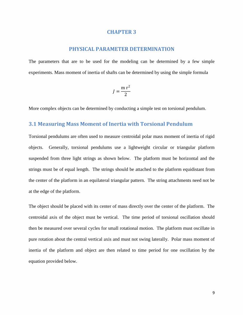
Torsional pendulums are often used to measure centroidal polar mass moment of inertia of rigid

objects. Generally, torsional pendulums use a lightweight circular or triangular platform

suspended from three light strings as shown below. The platform must be horizontal and the

strings must be of equal length. The strings should be attached to the platform equidistant from

the center of the platform in an equilateral triangular pattern. The string attachments need not be

at the edge of the platform.

The object should be placed with its center of mass directly over the center of the platform. The

centroidal axis of the object must be vertical. The time period of torsional oscillation should

then be measured over several cycles for small rotational motion. The platform must oscillate in

pure rotation about the central vertical axis and must not swing laterally. Polar mass moment of

inertia of the platform and object are then related to time period for one oscillation by the

equation provided below.

10

This procedure should be used first with an empty platform to determine the mass moment of the

platform itself and then repeated with the object centered on the platform to measure the mass

moment of the object plus the platform [9].

𝐽o + 𝐽p =g mo +mp r2 τ2

4s𝜋2

Fig 3.1 Torsional Pendulum

3.2 Mass moment of inertia calculation of axle shaft

The axles that connect the wheels are made of steel and have an outer diameter of 0.5 in and are

of length 12 in.

Volume = 𝑉 = 𝜋 r2 l = 𝜋 ∗ 0.252 ∗ 12 = 2.3562 in3

Denisty of steel = 𝜌 =0.28lb

in3

Mass = 𝜌 𝑉 = 0.28 ∗ 2.3562 = 0.6597 lb

𝐽 =m r2

2=

0.6597 ∗ 0.252

2= 0.0206 lbin2

s

r

11

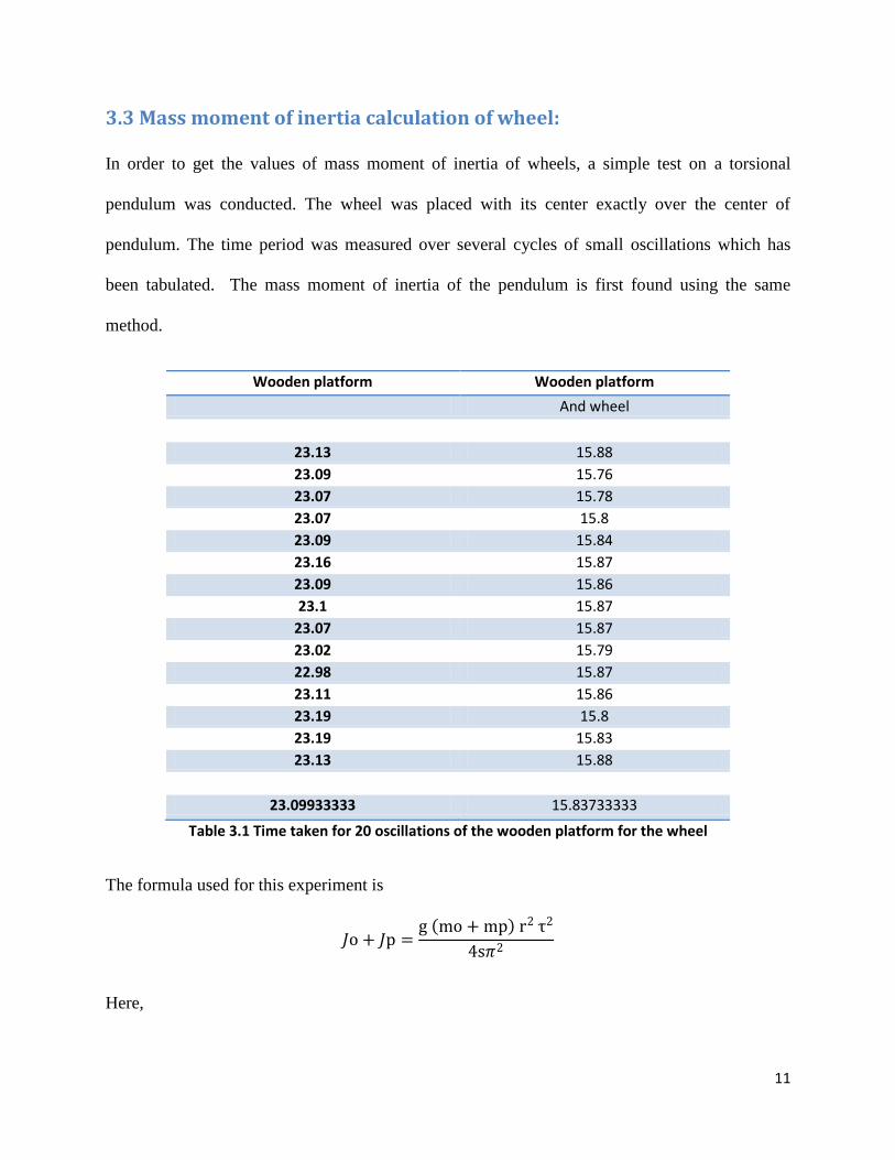
3.3 Mass moment of inertia calculation of wheel:

In order to get the values of mass moment of inertia of wheels, a simple test on a torsional

pendulum was conducted. The wheel was placed with its center exactly over the center of

pendulum. The time period was measured over several cycles of small oscillations which has

been tabulated. The mass moment of inertia of the pendulum is first found using the same

method.

Wooden platform Wooden platform

And wheel

23.13 15.88

23.09 15.76

23.07 15.78

23.07 15.8

23.09 15.84

23.16 15.87

23.09 15.86

23.1 15.87

23.07 15.87

23.02 15.79

22.98 15.87

23.11 15.86

23.19 15.8

23.19 15.83

23.13 15.88

23.09933333 15.83733333

Table 3.1 Time taken for 20 oscillations of the wooden platform for the wheel

The formula used for this experiment is

𝐽o + 𝐽p =g mo + mp r2 τ2

4s𝜋2

Here,

12

g = 32.2 ft/s2

mO = 2.48 lb.

mP = 1.002 lb.

r = 5.5 inch.

s = 21.3125 inch.

The time period of the wooden platform alone is τ = 1.1549666667 s.

Using the formula mentioned above the mass moment of inertia of the wooden platform is

computed to be

18.56088173 lb-in2

The time period of the wooden platform along with the wheels is τ = 0.798167 s.

Using the formula mentioned above the mass moment of inertia of the wheel is computed to be

11.75688242 lb-in2

3.4 Mass moment of inertia calculation of sprockets:

Similarly the mass moment of inertia of sprockets was found using another torsional pendulum

and the measured time period is tabulated.

mO1 = 0.11596 lb.

mO2 = 0.63317 lb.

mP = 0.3375 lb.

13

r = 2.752 inch.

s = 22.25 inch.

Metal platform Metal platform Metal platform

And Sprocket 1 And Sprocket 2

23.09 20.19 15.27

23.2 20.12 15.25

23.18 20.27 15.2

23.09 20.33 15.19

23.32 20.23 15.2

23.41 20.13 15.13

23.4 20.09 15.25

23.09 20.22 15.12

23.24 20.2 15.48

23.13 20.07 15.34

23.12 20.24 15.47

23.22 20.22 15.28

23.17 20.16 15.43

23.27 20.17 15.27

23.03 20.17 15.38

23.06 20.14 15.28

23.18875 20.184375 15.28375

Table 3.2 Time taken for 20 oscillations of the metal platform for the sprockets

The time period of the platform alone is τ = 1.1594375 s.

Using the formula mentioned above the mass moment of inertia of the metal platform is

computed to be 1.5138 lb-in2

The time period of the platform along with sprocket 1 is τ = 1.00921875 s.

Using the formula mentioned above the mass moment of inertia of sprocket 1 is computed to be

24.9375 * 10-3

lb-in2

14

The time period of the platform along with sprocket 2 is τ = 0.7641875 s.

Using the formula mentioned above the mass moment of inertia of sprocket 2 is computed to be

0.37425 lb-in2

3.5 Mass moment of inertia calculation of chain 1:

The chain that connects the two 10 tooth sprockets is called the Chain 1 and the mass moment of

inertia of chain is calculated under the assumption that mass of the chain is a point mass rotating

on the sprockets. The chain used is an ANSI #35 Chain.

The chain that was used for this purpose was of length = 20.25 in + (10 * 0.375) = 24 inch.

Mass of the chain = 0.21 ∗24

12= 0.42 lb

𝐽 = m r2 = 0.42 ∗ 0.5052 = 0.1071 lbin2

3.6 Mass moment of inertia calculation of chain 2:

The chain that connects the 10 tooth sprocket and the 20 tooth one is called the Chain 2 and the

mass moment of inertia of chain is calculated under the assumption that mass of the chain is a

point mass rotating on the sprockets. The chain used is an ANSI #35 Chain.

The chain that was used for this purpose was of length = 18 in + (12 * 0.375) = 22.5 inch.

Mass of the chain = 0.21 ∗22.5

12= 0.4125 lb

𝐽 = m r2 = 0.4125 ∗ 0.5052 = 0.1052 lbin2

15

CHAPTER 4

ADAMS SIMULATIONS AND RESULTS

This section presents the solid modeling and the dynamic simulations that were performed under

various conditions. These simulations were done with a view to assist modeling and also verify

the same. Adams (Automated Dynamic Analysis of Mechanical Systems) was used to do solid

modeling and the dynamic simulations. Adams is dynamic analysis software that models and

solves simultaneous equations for kinematic, static, quasi-static and dynamic simulations.

The parts that have the most significant influence on differential torque steer dynamics were

modeled - wheels, tires, frame, terrain, motors and axles. Vehicle model parameters (to scale) are

provided in APPENDIX A. Terrain modeling can be done to simulate reality using coefficients

of static friction, kinematic friction, and cohesion and pressure angle to include soil mechanics.

In this thesis, the terrain properties modeled are that of normal roads using friction model.

Adams was chosen because of its superior tire modeling which is one of the most important

parameter in skid steer dynamics. Adams‟s tire modeling has a module that includes vertical

direction modeling and it is superior to all other linear spring models. Tire damping has been

included in our modeling and they are not merely extrapolated from steady state data. Tire

longitudinal forces, lateral forces and aligning moments are complex non linear functions of pre

normal force, slip, slip angles, and tire road friction coefficient unlike other linear spring models.

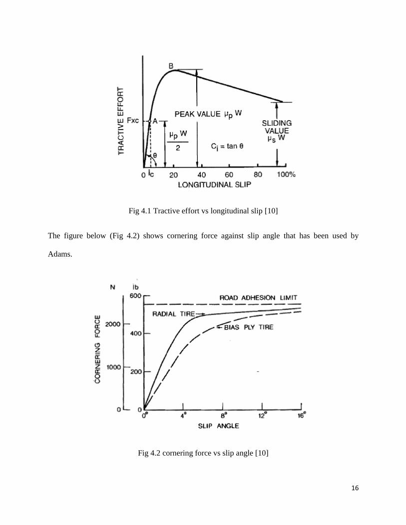
The tractive effort against longitudinal slip that has been used by Adams is as shown in the

figure below (Fig 4.1).

16

Fig 4.1 Tractive effort vs longitudinal slip [10]

The figure below (Fig 4.2) shows cornering force against slip angle that has been used by

Adams.

Fig 4.2 cornering force vs slip angle [10]

17

The motors can also be modeled in Adams, which is not easy in most other analysis software.

Solid body modeling plays a crucial role.

4.1 Simulations

4.1.1 Straight line maneuvers

4.1.1.1 On flat road

In order to achieve a straight line, the same torque was provided on both sides. The torque was

increased to 11 lbf-inch over 1 second and held for 5 seconds as shown in the figure below (Fig

4.3).

Fig 4.3 Input torque applied to the wheels (Straight line on a flat road)

X axis – time (in seconds)

Y axis – torque (in lbf-inch)

The simulated distance travelled by the vehicle was 906 inch. This was measured by plotting the

displacement of the center of gravity during the entire simulation, which is shown in Fig 4.4.

18

Fig 4.4 Distance travelled by the vehicle (Straight line on a flat road)

4.1.1.2 Accelerating on flat road

In order to achieve this simulation, the torque applied on both sets of wheels must be the same,

and increasing. The applied torque to achieve this maneuver was increased linearly to 31.25 lbf-

inch over 5 seconds. The input torque profile on all wheels is shown in Fig 4.5.

Fig 4.5 Input torque applied to the wheels (Accelerating on flat road)



19

The simulated distance travelled by the vehicle was 895 inch. This distance was obtained in the

same way as before from the following graph, Fig 4.6.

Fig 4.6 Distance travelled by the vehicle (Accelerating on flat road)

4.1.1.3 Accelerating on a ramp

In order to test the behavior of the vehicle in a slope, a ramp of 2 degrees was created and it was

made to move on a straight line by applying equal torque on both wheels. The applied torque was

increased linearly to 31.25 lbf-inch over 5 seconds. The input torque on each set of wheels is

shown in Fig 4.7.

20

Fig 4.7 Input torque applied to the wheels (Accelerating on a ramp)



The simulated distance travelled by the vehicle was 760 inch. This distance was obtained in the

same way as shown in Fig 4.8.

Fig 4.8 Distance travelled by the vehicle (Accelerating on a ramp)

21

4.1.1.4 Running over an oblique bump

In order to perform a simulation of the vehicle hitting an oblique bump (height of bump – 2 inch,

angle of the bump – 6 degrees) while travelling on a straight line, the torque applied on both

sides of the vehicle was increased to 9 lbf-inch over 1 second and held for 5 seconds to get to an

axle speed of 275 rpm. The vehicle rolled over when applied with a higher torque. The input

torque profile is shown below in Fig 4.9.

Fig 4.9 Input torque applied to the wheels (Running over an oblique bump)



The simulated distance travelled by the vehicle was 1115 inch as shown below in Fig 4.10.

22

Fig 4.10 Distance travelled by the vehicle (Running over an oblique bump)

The path of the vehicle is shown in Fig 4.11.

Fig 4.11 Path traced by the vehicle (Running over an oblique bump)

4.1.1.5 Running over a straight bump

In order to run this simulation, the same torque is to be applied on both sets of wheels and a road

with a straight bump of about 1 inch height was used. The torque applied was increased to 15

lbf-inch over 1 second and held for 5 seconds to get an axle speed of 455 rpm. The vehicle hit

23

the bump at this speed and was still stable. The vehicle rolled over on hitting the same bump

when the axle speed was increased above 550 rpm.

The input torque profile applied on the wheels is shown below in Fig 4.12.

Fig 4.12 Input torque applied to the wheels (Running over a straight bump)



The simulated distance travelled by the vehicle was 953 inch as shown in Fig 4.13.

Fig 4.13 Distance travelled by the vehicle (Running over a straight bump)

24

The path traced by the vehicle is shown in Fig 4.14.

Fig 4.14 Path traced by the vehicle (Running over a straight bump)

4.1.2 Circular motion


This simulation was done to see if the vehicle rolls over carrying heavy weights. The mass center

of the vehicle in this case was moved up by 5 inches. Torque applied on one set of wheels was

increased to 15.9 lbf-inch over 1 second, held for 8 seconds, and brought down to 0 again as

shown in Fig 4.15. On the other side, it was maintained at zero.

25

Fig 4.15 Input torque applied to one set of wheels (Circular motion on flat road)




Fig 4.16 Distance travelled by the vehicle (Circular motion on flat road)


26

Fig 4.17 Path traced by the vehicle (Circular motion on flat road)

The simulation produces axle speeds up to 398 rpm. Higher torque shown in Fig 4.18 produced

axle speeds up to 563 rpm at which the vehicle overturned.

Fig 4.18 Input torque applied to the wheels (Circular motion on flat road)



The simulated distance travelled was 1108 inch as shown in Fig 4.19.

27

Fig 4.19 Distance travelled by the vehicle (Circular motion on flat road)


Fig 4.20 Path traced by the vehicle (Circular motion on flat road)

4.1.2.2 On a ramp

This simulation was done to test the vehicle‟s behavior during a turn when it is moving on a

ramp with a slope of 2 degrees, which will be useful to test obstacle avoidance on a ramp. In

order to achieve this motion a torque of 15.9 lbf-inch was increased over 1 second, held for 8

28

seconds, and brought down to 0 again on one side of the vehicle as shown in Fig 4.21. The other

side was held at zero. The vehicle over turned at an axle speed of about 530 rpm on this ramp.

Fig 4.21 Input torque applied to one set of wheels (Circular motion on a ramp)




Fig 4.22 Distance travelled by the vehicle (Circular motion on a ramp)


29

Fig 4.23 Path traced by the vehicle (Circular motion on a ramp)

4.1.3 Lane change maneuver

In order to achieve a lane change maneuver the torque on one set of wheels was decreased while

the other was held at maximum and vice versa. The torque that was applied was 10.5 lbf-inch

increased over 1 second and held for 4 seconds on the right set of wheels. The same value was

applied on the left set of wheels but was held for only 3 seconds and then dropped to 0 over one

second and back up again on both the wheels. The entire simulation was run for 6 seconds, to

achieve an axle speed of 430 rpm. The vehicle rolled over when the same maneuver was

performed at an axle speed of 510 rpm.

The profile that was used for the motor torque on the left set of wheels is shown in Fig 4.24.

30

Fig 4.24 Input torque applied to the left set of wheels (Lane Change maneuver)



The profile that was used for the motor torque on the right set of wheels is shown below in Fig

4.25.

Fig 4.25 Input torque applied to the right set of wheels (Lane Change maneuver)




31

Fig 4.26 Path traced by the vehicle (Lane Change maneuver)

4.1.4 J- Turn maneuver

In order to achieve a j-turn maneuver, which will be extremely useful in obstacle avoidance, the

torque applied on one set of wheels must be reduced and increased.

Torque on the left set of wheels was increased to 11.5 lbf-in over 1 second and held for 4

seconds. It was reduced and the right set of wheels were held for 3 seconds and reduced to 0 and

maintained there. This simulation was run for 6 seconds to get an axle speed of about 415 rpm.

The vehicle over turned when the same maneuver was performed at an axle speed of 530 rpm.

The input torque profile on the left set of wheels is shown below in Fig 4.27.

32

Fig 4.27 Input torque applied to the left set of wheels (J-Turn maneuver)



The input torque profile on the right set of wheels is shown in Fig 4.28.

Fig 4.28 Input torque applied to the right set of wheels (J-Turn maneuver)



The simulated distance travelled by the vehicle was 867 inch as shown in Fig 4.29

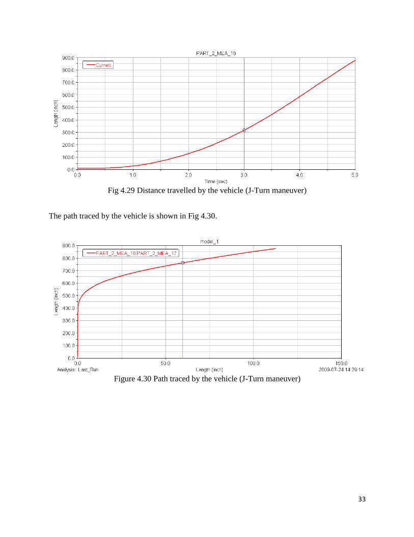
33

Fig 4.29 Distance travelled by the vehicle (J-Turn maneuver)


Figure 4.30 Path traced by the vehicle (J-Turn maneuver)

34

CHAPTER 5

MATLAB MODELING AND SIMULATION

Dynamic behavior of any vehicle is determined by the forces imposed on it from the tires,

gravity and aerodynamics. Conventions used to describe motion and forces in any model must be

uniform. Thus SAE Vehicle Axis System [10] has been used throughout. A lumped mass

approximation which has been used in this work is widely accepted under this system. In this, a

vehicle is assumed to behave as a single component (i.e. all components move together). The

mass of such a system is placed on the centre of gravity with appropriate mass and inertia

properties. Vehicle model parameters (to scale) are provided in APPENDIX A.

Two types of co-ordinate systems were used:

a) Vehicle Fixed Co-ordinate system

b) Earth Fixed Co-ordinate system

A vehicle fixed co-ordinate system has been used as shown in Fig 5.1. In this system, the

forward/longitudinal motion is represented by „x‟, right lateral motion by „y‟, downward

direction by „z‟. The rotations about these three axes are roll, pitch and yaw respectively. The

velocities are referenced to the earth fixed coordinate system as shown in Fig 5.2.

35

Fig 5.1 Vehicle fixed co-ordinate system in different views.

Vehicle in Earth Fixed Coordinate System is shown in Fig 5.2:

Y

Z FRONT

D

G

X

Z LEFT

D

G

X

Y

TOP

HLF HLM

HRF HRM

HLA

HRA

D G

36

Fig 5.2 Vehicle in earth-fixed co-ordinate system [11]

5.1 Tire modeling

Vehicle dynamic modeling also requires modeling of tires. Before getting into the details of

mechanics of force generation or the importance of modeling of tires, basic terminology and tire

axis system must be established as shown in Fig 5.3.

Fig 5.3 Tire axis system nomenclature [12]

37

Rolling resistance moment acts on the tire by the road, in the plane of the road and normal to the

intersection of the wheel plane with the road plane. Overturning moment acts on the tire by the

road in the plane of the road and is parallel to the intersection of the wheel plane with the road

plane.

5.2 Friction consideration

5.2.1 Mechanics of force generation

The forces on a tire are not applied at a point, but are the resultant from normal and shear

stresses distributed in the contact patch. The pressure distribution under a tire is not uniform as

shown in Fig 5.4. When rolling, it is generally not symmetrical about the Y-axis but tends to be

higher in the forward region of the contact patch. While modeling, the tractive properties of the

tire are to be taken into account.

Fig 5.4 Tire deformation mechanism [11]

38

The acceleration and braking forces are generated by producing a differential between the tire

rolling speed and its speed of travel. The consequence is production of slip in the contact patch.

Slip % = 1 −r ω

V 100

A good understanding of brake force versus slip plots is necessary for vehicle modeling. Under

typical braking conditions the longitudinal forces will vary with slip as shown in Fig 5.5 and Fig

5.6.

Fig 5.5 Friction force vs Slip [11]

39

Fig 5.6 Braking effort coefficient vs Slip [1]

From these above graphs we can see that the braking effort coefficient hits a maximum at about

20% slip and then dips down. In this work it has been modeled as a straight line that hits

maximum at the same 20% slip and then remains at that value. This is a reasonable assumption

often made in vehicle dynamic analyses. Tire rolling resistance was neglected in this model.

5.3 Dynamic Equations

As two different co-ordinate systems were used in this work, there must be a rotation matrix that

is used to transfer all the information from one to another. The rotation matrix to change from

local co-ordinate system to a global co-ordinate system will be of the following form.

𝐴 = 𝐴𝑧ψ 𝐴𝑦𝜃 𝐴𝑥𝜑

Global angular velocities are obtained from the local angles by using the matrix formula shown

below:

40

𝜔𝑥

𝜔𝑦

𝜔𝑧

= 00ψ + 𝐴𝑧ψ

0𝜃

0 + 𝐴𝑦𝜃 𝐴𝑧ψ

𝜑 00

Where

𝐴𝑧ψ = 𝑐ψ −𝑠ψ 0𝑠ψ 𝑐ψ 00 0 1

𝐴𝑦𝜃 = 𝑐𝜃 0 𝑠𝜃0 1 0

−𝑠𝜃 0 𝑐𝜃

𝑐𝜃 = cos 𝜃

𝑠𝜃 = sin 𝜃

Using these, the final matrix formula can be computed to be:

𝜔𝑥

𝜔𝑦

𝜔𝑧

= 𝑐ψ 𝑐𝜃 −𝑠ψ 0𝑠ψ 𝑠𝜃 𝑐ψ 0−𝑠𝜃 0 1

𝜑

𝜃

ψ

The matrix form equation can also be inverted and used to get from the global to local angular

velocities. The final expression for which is as follows:

𝜑

𝜃

ψ =

1

𝑐𝜃

𝑐𝜃 𝑠𝜃 𝑠𝜑 𝑠𝜃 𝑐𝜑0 𝑐𝜃 𝑐𝜑 −𝑐𝜃 𝑠𝜑0 𝑠𝜑 𝑐𝜑

𝜔𝑥

𝜔𝑦

𝜔𝑧

41

This work used a state space model. The state variables chosen in this work are:

Rg2 – location of center of gravity; the three angular co-ordinates ψ, 𝜃 and 𝜑 and their respective

first and second order derivatives.

The other important transformation is to translate data from the centre of gravity to the origin.

Here in this work, the centre of gravity and the origin are marked by points G and D as shown in

Fig 5.7.

Fig 5.7 Vehicle showing its centre of gravity and origin.

The output torque for a brushed DC motor using an electronic speed controller is shown below

where throttle command TC can vary between -1 (reverse) and +1 (forward)

𝑇𝑚𝑜𝑡𝑜𝑟 = 𝑇𝑚𝑎𝑥 𝑇𝐶 − 𝜔𝑚𝑜𝑡𝑜𝑟

𝜔𝑚𝑎𝑥

X

Z LEFT

D

G

42

5.4 Simulations

5.4.1 Straight line maneuvers


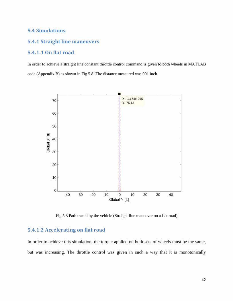
In order to achieve a straight line constant throttle control command is given to both wheels in MATLAB

code (Appendix B) as shown in Fig 5.8. The distance measured was 901 inch.

Fig 5.8 Path traced by the vehicle (Straight line maneuver on a flat road)

5.4.1.2 Accelerating on flat road

In order to achieve this simulation, the torque applied on both sets of wheels must be the same,

but was increasing. The throttle control was given in such a way that it is monotonically

-40 -30 -20 -10 0 10 20 30 400

10

20

30

40

50

60

70X: -1.174e-015

Y: 75.12

Global Y [ft]

Glo

bal X

[ft

]

43

increasing. The path of vehicle is shown in Fig 5.9 and the distance travelled by the vehicle was

891 inches which matches the Adams simulations (895 inches) in section 4.1.1.1.

Fig 5.9 Path traced by the vehicle (Accelerating on a flat road)

5.4.1.3 Accelerating on a ramp

In order to test the behavior of the vehicle in a slope, a ramp of 2 degrees was created and it was

made to move on a straight line by applying equal torque on both set of wheels. The throttle

command was similar to the one in the previous run. The distance travelled was 776 inch as

shown in the Fig 5.10, which is comparable to 761 inches from Adams simulation in Section

4.1.1.2.

-40 -30 -20 -10 0 10 20 30 400

10

20

30

40

50

60

70 X: 9.478e-016

Y: 74.26

Global Y [ft]

Glo

bal X

[ft

]

44

Fig 5.10 Path traced by the vehicle (Accelerating on a ramp)

5.4.2 Lane change maneuver

In order to achieve a lane change maneuver the torque on one set of wheels decreases when the other is

held constant and vice versa. The throttle command increased the axle speed up to 430 rpm over 1 second

and was held for 4 seconds on the right set of wheels. The left set of wheels were held for only 3 seconds

and then dropped to 0 in one second and back up again on both the wheels as shown in Fig 5.11. The

vehicle over turned when the same maneuver was performed at an axle speed of 510 rpm, which matched

Adams simulations in Section 4.1.3.

-40 -30 -20 -10 0 10 20 30 40

0

10

20

30

40

50

60X: 7.469e-016

Y: 64.65

Global Y [ft]

Glo

bal X

[ft

]

45

Fig 5.11 Input torque applied to the left and right set of wheels (Lane change maneuver).

Fig 5.12 shows the path traced by the vehicle during this maneuver.

0 2 4 60

0.5

1Throttle LEFT

time (in sec)

Thro

ttle

Com

mand

0 2 4 60

0.5

1Throttle RIGHT

time (in sec)

Thro

ttle

Com

mand

0 2 4 60

100

200

300

400

500

time (in sec)

[rpm

]

Wheels LEFT

0 2 4 60

100

200

300

400

500

time (in sec)

[rpm

]

Wheels RIGHT

46

Fig 5.12 Path traced by the vehicle (Lane change maneuver)

Fig 5.13 below shows that the tire forces from the ground fall to zero when this maneuver is

performed at axle speed above 510 rpm.

-20 0 20 40 60 80 100 120

0

100

200

300

400

500

600

Global Y [inch]

Glo

bal X

[in

ch]

47

Fig 5.13 Tire forces (Lane change maneuver, 510 rpm axle speed)

5.4.3 J- turn maneuver

The value of maximum throttle command in this case was 0.83. The left set of wheels were

increased to this value in 1 second and held for 4 seconds as shown in Fig 5.14. The right set of

wheels were held at the maximum throttle command for 3 seconds and then to 0 and maintained

there. This simulation was run for 6 seconds to get an axle speed of about 415 rpm. The vehicle

rolled over when the same maneuver was performed at an axle speed of about 530 rpm.

0 1 2 3 4 5 6-100

-50

0

50

100

time (in sec)

Forc

e [

lbf]

Tire LF

safe operation

wheels off the ground - unsafe

0 1 2 3 4 5 6-100

-50

0

50

100

time (in sec)

Forc

e [

lbf]

Tire RF

0 1 2 3 4 5 6-100

-50

0

50

100

time (in sec)

Forc

e [

lbf]

Tire LM

0 1 2 3 4 5 6-100

-50

0

50

100

time (in sec)

Forc

e [

lbf]

Tire RM

0 1 2 3 4 5 6-100

-50

0

50

100

time (in sec)

Forc

e [

lbf]

Tire LA

0 1 2 3 4 5 6-100

-50

0

50

100

time (in sec)

Forc

e [

lbf]

Tire RA

48

Fig 5.14 Input torque applied to the left and right set of wheels (J-turn maneuver).

The path traced by the vehicle during this maneuver is shown in Fig 5.15.

0 2 4 60

0.5

1Throttle LEFT

time (in sec)

Thro

ttle

Com

mand

0 2 4 60

0.5

1Throttle RIGHT

time (in sec)

Thro

ttle

Com

mand

0 2 4 60

100

200

300

400

500

time (in sec)

[rpm

]

Wheels LEFT

0 2 4 60

100

200

300

400

500

time (in sec)

[rpm

]

Wheels RIGHT

49

Fig 5.15 Path traced by the vehicle (J-turn maneuver)

-20 -10 0 10 20 30

0

5

10

15

20

25

30

35

40

45

Global Y [ft]

Glo

bal X

[ft

]

50

CHAPTER 6

CONCLUSION AND FUTURE WORK

A differential torque steer model was developed analytically and dynamic analysis was also

performed in Adams. Mathematical modeling was done for six wheel differential torque steer

using a six wheel model where the right and left axle torques were independent inputs. A

MATLAB simulation was performed. The Adams program for multi – body systems was also

used for the modeling, analysis, and animation.

Comparing the results of J-turn maneuver and Straight line maneuver on flat road (distance

travelled - 600 inch vs 901 inch), it can be seen that skidding causes excessive slip in tires. This

comparison can be made because, both the simulations were run for same amount of time and the

maximum throttle commands were the same. Skidding demands more power input but allows

zero turn radius which is impossible in other classes of steering systems. Considering the nature

of the terrain on which the AGV operates, power requirements will be high and tire wear will be

greater.

Based on the simulations performed on flat road and ramp the maximum difference in distance

travelled had a deviation of 1.9% (776 inches vs 761 inches). This may be attributed to the lack

of tire rolling resistance in the MATLAB model. The simulations that were performed on the

lane change and J-turn maneuver validates the accuracy of the dynamic details of the model. The

Axle speed at which the vehicle overturns, matched exactly in both the models.

51

6.1 Scope for Future Research

Further work needs to be done to refine the dynamic model to simulate curve motions. A better

friction model between the tires and the ground may lead to a more accurate simulation, while

the vehicle is skidding. Although the Adams model can provide better results, the mathematical

model is of more importance due to its proposed use in control for real-time prediction of

overturn events. The Adams model results can be used to refine the analytical model. The

vehicle model developed here is without a suspension system. Suspension may be needed for

high speed operation.

52

REFERENCES

1. Theory of Ground Vehicles, Wong

2. L. Mangialardi, “Study of the Horizontal Plane Motion of a Skid-Steering Vehicle,”

Proceedings of 7th

International Conference of ISTVS, pp. 1448 – 1472, Calgary, Alberta,

Canada, 1981.

3. A. Gentile and L. Mangialardi, “Behavior of a Non-Conventional Transmission and Skid-

Steering Vehicle,” Proceedings of 19th

International FISITA Congress: Energy Mobility,

Melbourne, Australia, SAEA Paper No. 82090, November 1982.

4. A. Gentile and L. Mangialardi, “Dynamic Steering Multiaxle Vehicles: Influence on

Axle-Numbers,” Proceedings of 20th

International FISITA Congress: The Automotive

Future, Vienna, Austria, SAE Report No. 845056, May 1984.

5. A.P.Creedy, “Skid Steering of Wheeled and Tracked Vehicles – Analysis with Coulomb

Friction Assumptions,” Engineering Development Establishment Report AR No 002.715,

Victoria, Australia, December 1984.

6. I. Schmid and W. Tomaske, “Power and Torque Requirements for Skid Steering

Vehicles,” Proceedings of ISTVS Conference on Off-Road Vehicles, FISITA 92, London,

U.K., pp. 216 – 230, June 1992.

7. C. Renou and S. Chavant, “A Computer Simulation Model for Skid-Steering of Non-

Directed Wheeled Vehicles,” Proceedings of 11th

International Conference of ISTVS, pp.

398 – 407, Lake Tahoe, Nevada, 1993.

8. Junnian Wang, Qingnian Wang and Liqiang Jin, “Modeling and Simulation Studies on

Differential Drive Assisted Steering for EV with Four-Wheel-Independent-Drive,” IEEE

Vehicle Power and Propulsion Conference (VPPC), September 3-5, 2008, Harbin, China.

53

9. Shigley, J.E. and J.J. Uicker, Theory of Machines and Mechanisms, McGraw-Hill, 1995,

second edition.

10. Tire and Vehicle Dynamics, Packeja

11. Fundamentals of Vehicle Dynamics, Thomas. D. Gillespie.

12. “Vehicle Dynamics Terminology”, SAE J670e, Society of Automotive Engineers,

Warrendale, PA.

54

APPENDIX A

MODEL PARAMETERS X [in] Y[in] Z[in]

D - design point 0 0 0

G - mass center -10.125 0 -10

HLF - hub left front 0 -8 0

HLM - hub left middle -10.125 -8 0

HLA - hub left aft -20.25 -8 0

HRF - hub right front 0 8 0

HRM - hub right middle -10.125 8 0

HRA - hub right aft -20.25 8 0

chassis LxWxH = 30x12x7 in

X

Y

TOP

HLF HLM

HRF HRM

HLA

HRA

D G

55

m = total mass of vehicle (including all tires) = 60 lbm

JG_XX = centroidal mass moment of vehicle at G in X direction = 965 lbm.in2

JG_YY = centroidal mass moment of vehicle at G in Y direction = 4745 lbm.in2

JG_ZZ = centroidal mass moment of vehicle at G in Z direction = 5220 lbm.in2

tire OD = unloaded diameter of tire = 8 inch

tire w = unloaded tire width = 2 inch

tire k = tire radial stiffness = 10 lbf/in

tire c = tire radial damping = 0.3 lbf.sec/in

tire μMAX = tire maximum adhesion = 0.8

Y

Z FRONT

D

G

X

Z LEFT

D

G

56

JT_YY = centroidal mass moment of one tire in Y direction = 11.8 lbm.in2

mT = mass of one tire = 2.5 lbm

ωMAX = maximum speed of motor = 500 rpm

TMAX = maximum torque from motor = 500 in.lbf

57

APPENDIX B

MATLAB Code

% sixwh_ini.m - initialize global constants % six wheel solid axle skid steer vehicle %

%%%%%%%%%%%%%%%%%%%%%%%%%%%%%%%%%%%%%%%%%%%%%%%%%%%%%%%%%%%%%%%%%%%%%%%%%%% % tire - assume all tires are identical tire.D = 8; % OD [inch] tire.R = tire.D / 2; % outside radius [in] tire.m = 3; % mass [lbm] J_approx = tire.m * tire.R * tire.R / 2; tire.J = J_approx; % mass moment [lbm.in2] %tire.k = 20; % radial stiffness [lbf/in] tire.k = 10; % radial stiffness [lbf/in] tire.c = 0.3; % radial damping [lbf.sec/in] tire.mu_s = 0.8; % sliding coefficient of adhesion tire.mu_rr = 0.15; % rolling reistance

% tire tractive Pacejka xm = 30; % [ips] yp = 0.8; ya = 0.75; D = yp; C = 1 + (1 - 2 * asin( ya/D ) / pi); slope = yp / (xm/2); B = slope /C /D; E = (B*xm - tan(pi/2/C)) / (B*xm - atan(B*xm)); tire.trac = [ B C D E ];

% tire lateral Pacejka xm = 30; % [ips] yp = 0.80; ya = 0.75; D = yp; C = 1 + (1 - 2 * asin( ya/D ) / pi); slope = yp / (xm/2); B = slope /C /D; E = (B*xm - tan(pi/2/C)) / (B*xm - atan(B*xm)); tire.lat = [ B C D E ];

% tire rolling resistance Pacejka xm = 1; % [ips] yp = 0.15; ya = 0.10; D = yp; C = 1 + (1 - 2 * asin( ya/D ) / pi); slope = yp / (xm/2); B = slope /C /D; E = (B*xm - tan(pi/2/C)) / (B*xm - atan(B*xm)); tire.rr = [ B C D E ];

58

%%%%%%%%%%%%%%%%%%%%%%%%%%%%%%%%%%%%%%%%%%%%%%%%%%%%%%%%%%%%%%%%%%%%%%%%%%% % motor - assume both motors are identical % M01 motors at 24V n_max = 500; % max speed [rpm] (about 3A) motor.w_max = n_max *2*pi /60; % [rad/sec] motor.T_max = 500; % stall torque [in.lbf] (about 120A) motor.T_drag = 10; % viscous drag torque on drive system

[in.lbf.sec]

%%%%%%%%%%%%%%%%%%%%%%%%%%%%%%%%%%%%%%%%%%%%%%%%%%%%%%%%%%%%%%%%%%%%%%%%%%% % ground - define as vertices and faces ground.gravity = 32.174*12 * [ 0 0 1 ]'; % gravity [ips2]

%%%%%%%%%%%%%%%%%%%%%%%%%%%%%%%%%%%%%%%%%%%%%%%%%%%%%%%%%%%%%%%%%%%%%%%%%%% % chassis % mass of chassis and tires m2 = 60; % [lbm] chassis.m2 = m2;

% mass moments of tire triplets % include mass moment for chains and sprockets JL = 3 * tire.J + 0; % [lbm.in2] JR = 3 * tire.J + 0;

% mass moments of chassis in body-fixed directions J2xx = m2*(12*12+7*7) / 12; % roll [lbm.in2] J2yy = m2*(30*30+7*7) / 12; % pitch [lbm.in2] J2zz = m2*(30*30+12*12) / 12; % yaw [lbm.in2]

% subtract tires from whole body Jyy J2yy = J2yy - JL - JR; chassis.J2_G2 = [ J2xx 0 0 ; 0 J2yy 0 ; 0 0 J2zz ];

% mass moments of tires chassis.JL = JL; % [lbm.in2] chassis.JR = JR;

% design point at midline of front axle % location of mass center for chassis and tires wrt design point chassis.sG2wrtD2_D2 = [ -10.125 0 -0 ]'; % [inch] centered fore/aft at

axle height

chassis.sG2wrtD2_D2 = [ -10.125 0 -10 ]'; % [inch] 10 in above axle

% location of tire hubs wrt design point chassis.sHLFwrtD2_D2 = [ 0 -8 0 ]'; % [in] chassis.sHLMwrtD2_D2 = [ -10.125 -8 0 ]'; chassis.sHLAwrtD2_D2 = [ -20.25 -8 0 ]';

59

chassis.sHRFwrtD2_D2 = [ 0 8 0 ]'; chassis.sHRMwrtD2_D2 = [ -10.125 8 0 ]'; chassis.sHRAwrtD2_D2 = [ -20.25 8 0 ]';

% unit direction for axles in body-fixed directions for positive tire

rotation chassis.u_L_G2 = [ 0 -1 0 ]'; % [non-dimensional] chassis.u_R_G2 = [ 0 -1 0 ]';

% bottom of sixwh_ini

%% sixwh_main03.m - six wheel skid steer solid axle UGV

% units [inch] [lbm] [lbf] [sec]

%% assumptions % SAE body-fixed coordinate frame - x forward, y right, z down % mass center attitude is the same as design point attitude % uses z(yaw)-y(pitch)-x(roll) Euler angles for attitude - pitch cannot be

+/- 90 deg % all tires are identical % cross moments of inertia for chassis are small % gyroscopic moments of tires are negligible % J for wheels should also include shafts and chains % spherical (not toroidal tire) geometry % no aligning moment caused by tire rotation about normal to ground % tractive and braking effrots are the same for tires % both motors are identical

% +++++++++++++++++++++++++++++++++++++++++++++++++++++++++++++ % debug % rolling resistance does not require any torque at steady state ??? % motor.T_drag = viscous % motor.T_drag = 0

%% clear

% global variables global chassis motor tire ground throttle keep

keep=[];

% constants d2r = pi / 180; r2d = 1 / d2r;

%% define global constants sixwh_ini

%% load throttle plan global constants sixwh_throttle

60

%% initial posture for design point - level ground

%rD2 = [ 0 0 -tire.R ]'; % zero tire deflection zD2 = -tire.R + chassis.m2/(6*tire.k); rD2 = [ 0 0 zD2 ]'; % static ride height

aG2 = [ 0 0 0 ]'; % Euler angles - phi roll local x % - theta pitch intermediate y % - psi yaw global z

% initial velocity for design point rdD2 = [ 0 0 0 ]'; wG2_G2 = [ 0 0 0 ]'; % angular velocity in body-fixed coordinates

% initial attitude matrix and Euler angle derivatives [ AG2, AdG2, adG2 ] = sixwh_makeA( aG2, wG2_G2 );

% initial position and velocity of G2 rG2 = rD2 + AG2 * chassis.sG2wrtD2_D2; rdG2 = rdD2 + AdG2 * chassis.sG2wrtD2_D2;

% initial angle and speed of tire triplets thL = 0; thR = 0;

thdL = 0; thdR = 0;

% 16x1 initial conditions for generalized coordinates y0 = [ rG2' aG2' thL thR rdG2' wG2_G2' thdL thdR ]';

% time range dt = 0.001; t_end = throttle.plan(end,1); time = ( 0 : dt : t_end )'; nt = length( time );

% allocate space y_all = zeros(nt,16);

% fixed step integration loop y = y0; for it = 1 : nt, t = time(it);

% t

yd = sixwh_yd( t, y );

% disp( 'yd' ) % disp( yd' ) % pause

61

y = y + yd*dt; y_all(it,:) = y'; if mod( it, 200 ) == 1, disp( t ) end end

xG2 = y_all(:,1)/12; % [ft] yG2 = y_all(:,2)/12; zG2 = -y_all(:,3); % [in]

thxG2 = y_all(:,4) * r2d; % roll [deg] thyG2 = y_all(:,5) * r2d; % pitch thzG2 = y_all(:,6) * r2d; % yaw

xdG2 = y_all(:,9) /12 /88 *60; % [mph] ydG2 = y_all(:,10) /12 /88 *60; % [mph] vG2 = sqrt( xdG2.*xdG2 + ydG2.*ydG2 ); zdG2 = -y_all(:,11); % [ips]

thdL = y_all(:,15)*60/2/pi; % [rpm] thdR = y_all(:,16)*60/2/pi;

%% Figures

% x-y trajectory figure( 1 ) clf iplot = ( 1 : 200 : nt )'; plot( yG2,xG2,'b', yG2(iplot),xG2(iplot),'ro' ) axis equal xlabel( 'Global Y [ft]' ) ylabel( 'Global X [ft]' )

figure( 2 ) clf subplot( 2, 2, 1 ) plot( time,vG2 ) ylabel( '[mph]' ) title( 'Forward velocity' )

subplot( 2, 2, 2 ) plot( time,thzG2 ) ylabel( '[deg CW from X]' ) title( 'Global heading (yaw)' )

subplot( 2, 2, 3 ) plot( time,thxG2 ) ylabel( '[deg]' ) title( 'Body-fixed roll' )

subplot( 2, 2, 4 ) plot( time,thyG2 ) ylabel( '[deg]' ) title( 'Pitch' )

62

% left wheel velocity, motor torque,torque control tcL = keep(:,1); tcR = keep(:,2);

TmotorL = keep(:,3); % [in.lbf] TmotorR = keep(:,4);

fCLF = keep(:,5); % [lbf] fCLM = keep(:,6); fCLA = keep(:,7);

fCRF = keep(:,8); fCRM = keep(:,9); fCRA = keep(:,10);

figure( 3 ) clf subplot( 3, 2, 1 ) plot( time, tcL ) title( 'Throttle LEFT' )

subplot( 3, 2, 2 ) plot( time, tcR ) title( 'Throttle RIGHT' )

subplot( 3, 2, 3 ) plot( time, TmotorL ) ylabel( 'Torque [in.lbf]' ) title( 'Motor LEFT' )

subplot( 3, 2, 4 ) plot( time, TmotorR ) ylabel( 'Torque [in.lbf]' ) title( 'Motor RIGHT' )

subplot( 3, 2, 5 ) plot( time, thdL ) ylabel( '[rpm]' ) title( 'Wheels LEFT' )

subplot( 3, 2, 6 ) plot( time, thdR ) ylabel( '[rpm]' ) title( 'Wheels RIGHT' )

figure( 4 ) clf subplot( 3, 2, 1 ) plot( time,fCLF,'b', time(fCLF==0),fCLF(fCLF==0),'ro' ) ylabel( 'Force [lbf]' ) title( 'Tire LF' )

subplot( 3, 2, 2 )

63

plot( time,fCRF,'b', time(fCRF==0),fCRF(fCRF==0),'ro' ) ylabel( 'Force [lbf]' ) title( 'Tire RF' )

subplot( 3, 2, 3 ) plot( time,fCLM,'b', time(fCLM==0),fCLM(fCLM==0),'ro' ) ylabel( 'Force [lbf]' ) title( 'Tire LM' )

subplot( 3, 2, 4 ) plot( time,fCRM,'b', time(fCRM==0),fCRM(fCRM==0),'ro' ) ylabel( 'Force [lbf]' ) title( 'Tire RM' )

subplot( 3, 2, 5 ) plot( time,fCLA,'b', time(fCLA==0),fCLA(fCLA==0),'ro' ) ylabel( 'Force [lbf]' ) title( 'Tire LA' )

subplot( 3, 2, 6 ) plot( time,fCRA,'b', time(fCRA==0),fCRA(fCRA==0),'ro' ) ylabel( 'Force [lbf]' ) title( 'Tire RA' )

function [ A, Ad, ad ] = sixwh_makeA( a, w_bf ) % make rotation matrix and derivatives % six wheel solid axle skid steer vehicle % HJSIII, 09.03.07 % % INPUTS - a = 3x1 Euler angles [ phi theta psi ]' % phi roll local x % theta pitch intermediate y % psi yaw global z % w_bf = 3x1 body-fixed angular velocity [ wx_bf wy_bf wz_bf ]' % % OUTPUTS - A = 3x3 attitude matrix % Ad = 3x3 time derivative of attitude matrix % ad = 3x1 time derivative of Euler angles

% attitude matrix and derivative phi_x = a(1); theta_y = a(2); psi_z = a(3); Az = [ cos(psi_z) -sin(psi_z) 0 ; sin(psi_z) cos(psi_z) 0 ; 0 0 1 ];

Ay = [ cos(theta_y) 0 sin(theta_y) ; 0 1 0 ; -sin(theta_y) 0 cos(theta_y) ];

Ax = [ 1 0 0 ; 0 cos(phi_x) -sin(phi_x) ;

64

0 sin(phi_x) cos(phi_x) ];

A = Az * Ay * Ax; Ad = A * skew_sym( w_bf );

% convert body-fixed angular velocity to derivatives of Euler angles T = [ cos(theta_y) sin(theta_y)*sin(phi_x) sin(theta_y)*cos(phi_x) ; 0 cos(theta_y)*cos(phi_x) -cos(theta_y)*sin(phi_x) ; 0 sin(phi_x) cos(phi_x) ]; T = T / cos(theta_y); ad = T * w_bf;

% bottom of sixwh_makeA

% sixwh_throttle.m - throttle control plan % six wheel solid axle skid steer vehicle

% t [sec], tcL [-1 to 1], tcR [-1 to 1]

% straight speed = 0.87; plan01 = [ 0.00 0 0 ; 2.00 speed speed ; % 2 sec, accelerate to full speed, straight 6.00 speed speed ; % 4 sec, hold full speed, straight 8.00 speed speed ]; % 2 sec, declerate to sero, straight

% J-turn - straight, hard right, stop speed = 0.90; plan02 = [ 0.00 0 0 ; 1.00 speed speed ; % 1 sec, accelerate to full speed, straight 3.00 speed speed ; % 2 sec, hold full speed, straight 4.00 speed speed ; % 1 sec, hold L full speed, cut R to zero 5.00 speed 0 ; 6.00 0 0 ]; % 1 sec, cut L to zero, hold R at zero

% S-turn - straight, hard right, hard left, resume speed = 1.02; plan03 = [ 0.00 0 0 ; 1.00 speed speed ; % 1 sec, accelerate to max, straight 3.00 speed speed ; % 2 sec, hold at max, straight 4.00 speed 0 ; % 1 sec, hold L at max, cut R to zero 5.00 0 speed ; % 1 sec, cut L to zero,acclerate R to max 6.00 speed speed ; % 1 sec, accelerate L to max, hold R at max 8.00 speed speed ]; % 2 sec, accelerate L to max, hold R at max

% plan02 - speed=1.0, zG2wrtD2=-10, k=20 - lift RM/RA % - speed=1.0, zG2wrtD2=-10, k=10 - complete overturn % - speed=0.99, zG2wrtD2=-10, k=10 - lift LA/RF/RM/RA % - speed=0.88, zG2wrtD2=-10, k=10 - lift RA

speed = 1.02;

65

plan04 = [ 0.00 0 0 ; 1.00 speed speed ; % 1 sec, accelerate to max, straight 3.00 speed speed ; % 2 sec, hold at max, straight 4.00 speed 0 ; % 1 sec, hold L at max, cut R to zero 5.00 0 speed ; % 1 sec, cut L to zero,acclerate R to max 6.00 speed speed ; % 1 sec, accelerate L to max, hold R at max 11.00 speed speed ]; % 2 sec, accelerate L to max, hold R at

max

throttle.plan = plan02;

% bottom of sixwh_throttle

function [ rC, fC ] = sixwh_tire( rH, rdH, w, u_axle ) % compute tire contact patch location and force % six wheel solid axle skid steer vehicle % % INPUTS - rH = 3x1 global location of wheel hub % rdH = 3x1 global velocity of wheel hub % w = 3x3 global angular velocity of wheel % u_axle = 3x1 global unit direction for axle % % OUTPUTS - rC = 3x1 global location of tire contact patch % fC = 3x1 global force on tire at contact patch


% constants eps = 1e-1; % small value for slip r2d = 180 / pi; % radians to degrees

% normal from tire hubs to ground

% need ground here % check from hub to planar patches % from hub to each edge % from hub to each vertex

% contact point for flat infinite ground % assumes spherical (not toroidal tire)

% contact point for a flat ramp temp = tand(2); z = - temp * rH(1); ramp = 0; if ramp == 0 rC = [ rH(1) rH(2) 0 ]'; else rC = [ rH(1) rH(2) z ]'; end

% effective rolling radius rho = rC - rH; Re = norm( rho );

66

if Re < tire.R,

% tire local directions if norm( w ) > 0.0001, VCwrtH = cross( w, rho ); % velocity of C on tire with respect to hub

due to rotation Vroll = norm( VCwrtH ); % pure rolling velocity else VCwrtH = cross( u_axle, rho ); % direction if w=0 Vroll = 0; end

u_nor = -unit( rho ); % normal direction (from ground to hub) u_rol = -unit( VCwrtH ); % rolling direction u_lat = cross( u_nor, u_rol ); % lateral direction

% hub velocity in tire local directions VH_nor = u_nor' * rdH; VH_rol = u_rol' * rdH; VH_lat = u_lat' * rdH;

% percent slip in rolling direction %{ den = max( [ Vroll abs(VH_Rol) ] ); if den > eps, slip = Vroll - VH_Rol; pct_slip = 100 * slip / den; else slip = 0; pct_slip = 0; end % lateral slip angle alpha_deg = atan( abs(VH_Lat) / Vroll ) * r2d; % rudimentary tire model mu_trac = min( [ tire.mu_s*pct_slip/20 tire.mu_s ] ); mu_lat = min( [ tire.mu_s*alpha_deg/20 tire.mu_s ] ); %}

% normalized tire forces with saturation V_max_trac = 30; % [ips] V_max_lat = 30; V_max_rr = 1;

slip = Vroll - VH_rol;

mu_trac = tire.mu_s * min( [ abs(slip)/V_max_trac 1 ] ); mu_lat = tire.mu_s * min( [ abs(VH_lat)/V_max_lat 1 ] ); mu_rr = tire.mu_rr * min( [ Vroll/V_max_rr 1 ] );

% tractive coefficient using Pacejka model B = tire.trac(1); C = tire.trac(2); D = tire.trac(3); E = tire.trac(4); x = abs(slip);

67

% mu_trac = D*sin( C*atan( B*x - E*(B*x-atan(B*x)) ) );

% lateral coefficient using Pacejka model B = tire.lat(1); C = tire.lat(2); D = tire.lat(3); E = tire.lat(4); x = abs(VH_lat); % mu_lat = D*sin( C*atan( B*x - E*(B*x-atan(B*x)) ) );

% rolling resistance coefficient using Pacejka model B = tire.rr(1); C = tire.rr(2); D = tire.rr(3); E = tire.rr(4); x = Vroll; % mu_rr = D*sin( C*atan( B*x - E*(B*x-atan(B*x)) ) );

% tire forces f_nor = tire.k * (tire.R-Re) - tire.c * VH_nor; % f_rol = mu_trac * f_nor * sign(slip) - mu_rr * f_nor; f_rol_trac = mu_trac * f_nor * sign(slip); f_rol_rr = - mu_rr * f_nor; f_rol = f_rol_trac + f_rol_rr; f_lat = -mu_lat * f_nor * sign(VH_lat);

%disp( [ slip f_rol_trac Vroll f_rol_rr ] ) %pause

% rotation about normal and steering torque w_nor = u_nor' * w; mu_r_steer = 0; % ????????????? m_nor = - mu_r_steer * f_nor * sign(w_nor);

% combined force fC = f_nor*u_nor + f_rol*u_rol + f_lat*u_lat;

% no contact else fC = [ 0 0 0 ]'; end

% bottom of sixwh_tire

function yd = sixwh_yd( t, y ) % derivatives of state variables % six wheel solid axle skid steer vehicle


% rip state variables into smaller terms rG2 = y(1:3); aG2 = y(4:6); thL = y(7);

68

thR = y(8);

rdG2 = y(9:11); wG2_G2 = y(12:14); thdL = y(15); thdR = y(16);

% current attitude matrix and Euler angle derivatives [ AG2, AdG2, adG2 ] = sixwh_makeA( aG2, wG2_G2 );

% angular velocity of chassis in global directions wG2 = AG2 * wG2_G2;

% axles and angular velocities of tires in global directions u_L = AG2 * chassis.u_L_G2; u_R = AG2 * chassis.u_R_G2;

wL = wG2 + thdL * u_L; wR = wG2 + thdR * u_R;

% global position and velocity of D2 rD2 = rG2 - AG2 * chassis.sG2wrtD2_D2; rdD2 = rdG2 - AdG2 * chassis.sG2wrtD2_D2;

% global position and velocity of tire hubs rHLF = rD2 + AG2 * chassis.sHLFwrtD2_D2; rHLM = rD2 + AG2 * chassis.sHLMwrtD2_D2; rHLA = rD2 + AG2 * chassis.sHLAwrtD2_D2;

rHRF = rD2 + AG2 * chassis.sHRFwrtD2_D2; rHRM = rD2 + AG2 * chassis.sHRMwrtD2_D2; rHRA = rD2 + AG2 * chassis.sHRAwrtD2_D2;

rdHLF = rdD2 + AdG2 * chassis.sHLFwrtD2_D2; rdHLM = rdD2 + AdG2 * chassis.sHLMwrtD2_D2; rdHLA = rdD2 + AdG2 * chassis.sHLAwrtD2_D2;

rdHRF = rdD2 + AdG2 * chassis.sHRFwrtD2_D2; rdHRM = rdD2 + AdG2 * chassis.sHRMwrtD2_D2; rdHRA = rdD2 + AdG2 * chassis.sHRAwrtD2_D2;

%%%%%%%%%%%%%%%%%%%%%%%%%%%%%%%%%%%%%%%%%%%%%%%%%% %t

% contact patch and force on each tire [ rCLF, fCLF ] = sixwh_tire( rHLF, rdHLF, wL, u_L ); [ rCLM, fCLM ] = sixwh_tire( rHLM, rdHLM, wL, u_L ); [ rCLA, fCLA ] = sixwh_tire( rHLA, rdHLA, wL, u_L );

[ rCRF, fCRF ] = sixwh_tire( rHRF, rdHRF, wR, u_R ); [ rCRM, fCRM ] = sixwh_tire( rHRM, rdHRM, wR, u_R ); [ rCRA, fCRA ] = sixwh_tire( rHRA, rdHRA, wR, u_R );

% show tire forces

69

%disp( 'contact forces' ) %disp( [ fCLF fCLM fCLA fCRF fCRM fCRA ] ) %pause

% summation of tire forces on chassis in global directions [lbf] sumF2 = fCLF + fCLM + fCLA + fCRF + fCRM + fCRA;

% summation of tire moments on chassis about centroid in global directions

[in.lbf] sumM2 = cross( rCLF-rG2, fCLF ) + cross( rCLM-rG2, fCLM ) + cross( rCLA-rG2,

fCLA ) ... + cross( rCRF-rG2, fCRF ) + cross( rCRM-rG2, fCRM ) + cross( rCRA-rG2,

fCRA );

% summation of moments on tire triplets about axles in global directions

[in.lbf] sumML = cross( rCLF-rHLF, fCLF ) + cross( rCLM-rHLM, fCLM ) + cross( rCLA-

rHLA, fCLA ); sumMR = cross( rCRF-rHRF, fCRF ) + cross( rCRM-rHRM, fCRM ) + cross( rCRA-

rHRA, fCRA );

% motor torques [in.lbf] tcL = interp1( throttle.plan(:,1), throttle.plan(:,2), t ); tcR = interp1( throttle.plan(:,1), throttle.plan(:,3), t ); TmotorL = motor.T_max * ( tcL - thdL / motor.w_max ); TmotorR = motor.T_max * ( tcR - thdR / motor.w_max );

%%%%%%%%%%%%%%%%%%%%%%%%%%%%%%%%%%%%%%%%%%%%% %if t>0.1, % TmotorL = 0; % TmotorR = 0; %end

keep = [ keep ; [ tcL tcR TmotorL TmotorR fCLF(3) fCLM(3) fCLA(3) fCRF(3)

fCRM(3) fCRA(3) ] ];

% summation of moments on tire triplets about axles in axle directions

[in.lbf] sumML_axleL = u_L' * sumML; sumMR_axleR = u_R' * sumMR;

% angular acceleration of tires %netML = sumML_axleL + TmotorL - motor.T_drag*sign(thdL); % [in.lbf] %netMR = sumMR_axleR + TmotorR - motor.T_drag*sign(thdR); %netML = sumML_axleL + TmotorL - motor.T_drag*thdL; % [in.lbf] %netMR = sumMR_axleR + TmotorR - motor.T_drag*thdR; netML = sumML_axleL + TmotorL; % [in.lbf] netMR = sumMR_axleR + TmotorR;

thddL = 32.174*12 * netML / chassis.JL; % [rad/sec2] thddR = 32.174*12 * netMR / chassis.JR;

% angular acceleration of chassis in body-fixed directions netM2 = sumM2 - netML*u_L - netMR*u_R; % global moments [in.lbf] netM2_G2 = AG2' * netM2; % body-fixed moments

70

wdG2_G2 = 32.174*12 * inv(chassis.J2_G2) * netM2_G2; % [rad/sec2]

% acceleration of chassis in global directions rddG2 = ( sumF2*32.174*12 + chassis.m2*ground.gravity ) / chassis.m2; %

[ips2]

% 16x1 derivatives of generalized coordinates yd = [ rdG2' adG2' thdL thdR rddG2' wdG2_G2' thddL thddR ]';

% bottom of sixwh_yd

function amat = skew_sym( avec ) % form skew symmetric matrix from vector % % USAGE % amat = skew_sym( avec ) % % INPUT % avec = 3x1 vector % % OUTPUT % amat = 3x3 matrix

amat = zeros(3,3); amat(1,2) = -avec(3); amat(1,3) = avec(2); amat(2,3) = -avec(1); amat(2,1) = avec(3); amat(3,1) = -avec(2); amat(3,2) = avec(1);

% bottom of skew_sym.m

function unit = unit( avec ) % form unit vector % % USAGE % unit = unit( avec ) % % INPUT % avec = 3x1 vector % % OUTPUT % unit = 3x1 matrix

n_vec = norm (avec); unit = avec/n_vec;

% bottom of unit.m

modeling and simulation of a six wheel differential …

Documents