modeling and simulation of sloshing motion … chongdong... · modeling and simulation of sloshing...
TRANSCRIPT
1
Aalesund University College
TITLE:
MODELING AND SIMULATION OF SLOSHING MOTION IN
PARTLY FILLED TANK
CANDIDATE NAME:
Dong,Chongdong 2101
DATE: COURSE CODE: COURSE TITLE: RESTRICTION:
29/05/2015 IP501909 MSc thesis, discipline oriented
STUDY PROGRAM: PAGES/APPENDIX: LIBRARY NO.:
Ship Design 86/5
SUPERVISOR(S):
Karl Henning Halse
ABSTRACT:
With the increasing consume of LNG all over the world, transport of LNG through sea becomes more and more
important. When LNG carrier is on wave with partly filled tank, sloshing will occur and cause damage to the
structure of tank, or affects vessel's ability. Sloshing load nowadays has become a important design parameters
as the fatigue consideration. To study this sloshing phenomenon, this thesis carried out a numerical method to
simulated the sloshing in partly filled LNG tank with different kinds of shapes, which are prismatic, rectangular
and cylindrical tanks.
The software STAR-CCM+ is used to model and simulated the sloshing motion, both two dimensional and three
dimensional models are involved. Four kinds of tank motions are considered: surge, sway, roll and pitch motion.
The tank is excited by a regular sin or cosine waves with natural frequency. Natural frequency of specific tanks
is calculated and confirmed. Different kinds of liquid filling levels 30%, 50% and 70% are included. Moreover,
the numerical results of the free surface movements are compared with the published experimental results and a
good agreement is obtained. In addition, three dimensional effects is found and discussed. Furthermore, some
inner structure--baffle is used to reduce the sloshing motion and compared.
This thesis is submitted for evaluation at Ålesund University College.
2
Aalesund University College
MASTER THESIS 2015
FOR
STUD.TECHN. CHONGDONG DONG
MODELING AND SIMULATION OF SLOSHING MOTION IN
PARTLY FILLED TANK
Background.
Sloshing motion occurs easily in partly filled tank, especially LNG tank and roll-reduction
tank. Nowadays with the increasing size of LNG tanks and other marine tanks, sloshing load
becomes more and more important as the fatigue consideration of the design parameters.
Different types of tank have different characteristics of sloshing motion. For LNG tanks,
surge and pitch motion of vessel will cause the largest sloshing motion while in roll-reduction
tanks are sway and roll motion. Then how to simulate and study this kind of sloshing motion
and improve the strength or performance of the tank becomes an important task.
Objectives.
This thesis will deal with modeling and simulation of the sloshing motion in partly filled tank.
The main objective is to develop a CFD model to study this phenomenon. The CFD approach
is good since theoretical and experimental method has its own limitation. In this thesis,
STAR-CCM+ will be used for modeling and simulation of the sloshing motion. We can study
and compare different kinds of tanks or inducing motions and understand the system well.
The thesis work shall include the following:
Pre-study
o LNG tank types and related ship motions.
o Knowledge of CFD method.
o State of the LNG tank models.
Develop a CFD model for dynamic simulation of the sloshing motion.
o Establish CFD models(shape, size, motion, etc)
o Define water as the test filling.
o Define LNG as the simulation filling.
Perform simulations and test models on various configurations
o Simulate varying filling degree
o Simulate varying presented motion
o Analyze simulation results - output pressure distribution, output graph of
phases and free surface and etc.

3
Aalesund University College
o Evaluate computational results and make suggestions for recommended
practice.
The scope of work may prove to be larger than initially anticipated. Subject to approval from
the advisor, topics from the list above may be deleted or reduced in extent.
The thesis should be written as a research report with summary, conclus ion, literature
references, table of contents, etc. During preparation of the text, the candidate should make
efforts to create a well arranged and well written report. To ease the evaluation of the thesis, it
is important to cross-reference text, tables and figures. For evaluation of the work a thorough
discussion of results is needed. Discussion of research method, validation and generalization
of results is also appreciated.
In addition to the thesis, a research paper for publication shall be prepared.
Three weeks after start of the thesis work, a pre-study have to be delivered. The pre-study
have to include:
Research method to be used
Literature and sources to be studied
A list of work tasks to be performed
An A3 sheet illustrating the work to be handed in.
A templates and instructions for thesis documents and A3-poster are available on the
Fronterwebsite under MSc-thesis. Please follow the instructions closely, and ask your
supervisor or program coordinator if needed.
The thesis shall be submitted in electronic version according to new procedures from 2014.
Instructions are found on the college web site. In addition one paper copy of the full thesis
with a CD including all relevant documents and files shall be submitted to your supervisor.
Supervision at AAUC: Karl H. Halse,
Contact at : Aalesund University College
Karl H. Halse
Supervisor
Delivery: 15.01.2015 Signature candidate: _Chongdong Dong______
4
Aalesund University College
PREFACE
This paper is the master thesis for the person in master of Ship Design programs. The topic comes
from the project in Rolls-Royce and related to the courses of Ship Design programs. The person
has the Naval architecture and Ocean Engineering Bachelor's degree in HUST and is the second
year of master student in Aalesund University College.
In the study of Msc thesis, Karl Henning Halse is the supervisor and a lot of help is get from him
such as the advice of simulation steps and checking of the results. Besides, Grotle Erlend Liavåg
also provides many suggestions focus on the model and thermal part of the simulation. Without
their help , this master thesis could not be finished completely. Thanks a lot to them!
In addition, friends and families' supports are also the motivation for the person to finish the
master's study and thesis. Thanks for their supports!
5
Aalesund University College
ABSTRACT
With the increasing consume of LNG all over the world, transport of LNG through sea becomes
more and more important. When LNG carrier is on wave with partly filled tank, s loshing will
occur and cause damage to the structure of tank, or affects vessel's ability. Sloshing load nowadays
has become a important design parameters as the fatigue consideration. To study this sloshing
phenomenon, this thesis carried out a numerical method to simulated the sloshing in partly filled
LNG tank with different kinds of shapes, which are prismatic, rectangular and cylindrical tanks.
The software STAR-CCM+ is used to model and simulated the sloshing motion, both two
dimensional and three dimensional models are involved. Four kinds of tank motions are
considered: surge, sway, roll and pitch motion. The tank is excited by a regular sin or cosine
waves with natural frequency. Natural frequency of specific tanks is calculated and confirmed.
Different kinds of liquid filling levels 30%, 50% and 70% are included. Moreover, the numerical
results of the free surface movements are compared with the published experimental results and a
good agreement is obtained. In addition, three dimensional effects is found and discussed.
Furthermore, some inner structure--baffle is used to reduce the sloshing motion and compared.
Key words: LNG tank; Sloshing; Prismatic, rectangular and cylindrical tank; Natural Frequency;
Three dimensional effects; Baffle.
6
Aalesund University College
Table of contents
1. Introduction ................................................................................................................. 8
1.1. Background and Purpose ....................................................................................... 8
1.1.1.Background................................................................................................. 8
1.1.2.Purpose ........................................................................................................... 10
1.2.Sloshing ..............................................................................................................11
1.3.Previous Research ............................................................................................... 12
1.3.1.Theoretical Analytic Method ....................................................................... 12
1.3.2. Numerical Method .................................................................................... 13
1.3.3.Experimental Method ................................................................................. 18
1.3.4.Fluid Structure Interaction........................................................................... 19
1.4.Summery of the Thesis ......................................................................................... 19
2.Overview of LNG Carrier and Tank Sloshing................................................................ 21
2.1.LNG Carrier ....................................................................................................... 21
2.1.1.Brief Introduction ...................................................................................... 21
2.1.2.Tank Types................................................................................................ 22
2.2.Overview of Sloshing in LNG Carrier .................................................................... 25
2.2.1.Feathers of Sloshing ................................................................................... 25
2.2.2.Prevention Methods ................................................................................... 26
3.Theoretical Analysis and Numerical Method ................................................................. 27
3.1.Theoretical Formulation ....................................................................................... 27
3.1.1.Governing Equations .................................................................................. 27
3.1.2.Boundary Conditions .................................................................................. 30
3.2.Method of Numerical Simulation of Sloshing .......................................................... 32
3.3.STAR-CCM+ ...................................................................................................... 33
4.Modeling and Simulation of Sloshing Tank ................................................................... 35
4.1.Model Description ............................................................................................... 35
4.1.1.Mesh ........................................................................................................ 35
4.1.2.Physics ..................................................................................................... 37
4.1.3.Solver, Monitoring and Reporting ................................................................ 39
4.2.Verif ication ......................................................................................................... 39
4.3.Natural Frequency ............................................................................................... 44
4.3.1.Transverse Direction .................................................................................. 44
4.3.2.Longitudinal Direction................................................................................ 49
4.4.Other effects ....................................................................................................... 52
4.4.1.Amplitude ................................................................................................. 52
4.4.2.Three Dimensional Effects .......................................................................... 53
4.5 Summary of the Chapter ....................................................................................... 55
5.Simulation for LNG Tank ............................................................................................ 56
5.1 Prismatic and Rectangular Tanks ........................................................................... 58
5.1.1. Two dimension ......................................................................................... 58
7
Aalesund University College
5.1.2 Baffle Effects ............................................................................................ 60
5.1.2.Three Dimension ....................................................................................... 65
5.2 Cylindrical Tank Simulation.................................................................................. 70
5.3 Summary of This Chapter ..................................................................................... 76
6.Summary .................................................................................................................... 77
6.1.Conclusion ......................................................................................................... 77
6.2.Shortage ............................................................................................................. 78
6.3.Future work ........................................................................................................ 78
7.Reference .................................................................................................................... 79
Appendix A .................................................................................................................... 81
Appendix B .................................................................................................................... 85
8
Aalesund University College
1. Introduction
1.1. Background and Purpose
1.1.1.Background
Natural gas is a fossil fuel formed when layers of buried plants, gases, and animals are exposed to
intense heat and pressure over thousands of years. It is a hydrocarbon gas mixture consisting
primarily of methane, but commonly includes varying amounts of other higher alkanes and
sometimes a usually lesser percentage of carbon dioxide, nitrogen, and/or hydrogen sulfide.
Natural gas is an energy source often used for heating, cooking, and electricity generation. It is
also used as fuel for vehicles and as a chemical feedstock in the manufacture of plastics and other
commercially important organic chemicals.
Liquefied natural gas (LNG) is natural gas (predominantly CH4) that has been converted to liquid
form for ease of storage or transport. It takes up about 1/600th the volume of natural gas in the
gaseous state. It is odorless, colorless, non-toxic and non-corrosive. The liquefaction process
involves removal of certain components, such as dust, acid gases, helium, water, and heavy
hydrocarbons, which could cause difficulty downstream. The natural gas is then condensed into a
liquid at close to atmospheric pressure by cooling it to approximately −162 °C (−260 °F) . LNG
achieves a higher reduction in volume than compressed natural gas (CNG) so that the (volumetric)
energy density of LNG is 2.4 times greater than that of CNG or 60 percent of that of diesel fuel.
This makes LNG cost efficient to transport over long distances where pipelines do not exist.
Specially des igned cryogenic sea vessels (LNG carriers) or cryogenic road tankers are used for its
transport. LNG is principally used for transporting natural gas to markets, where it is regasified
and distributed as pipeline natural gas.
The LNG industry developed slowly during the second half of the last century because most LNG
plants are located in remote areas not served by pipelines, and because of the large costs to treat
and transport LNG. In the early 2000s, prices for constructing LNG plants, receiving terminals
and vessels fell as new technologies emerged and more players invested in liquefaction and
regasification. This tended to make LNG more competitive as a means of energy distribution, but
increasing material costs and demand for construction contractors have put upw ard pressure on
prices in the last few years.
Recently, with the increasing price of the crude oil and concern of environmental pollution, LNG
9
Aalesund University College
becomes more and more important as a relative economical and environmentally friendly energy
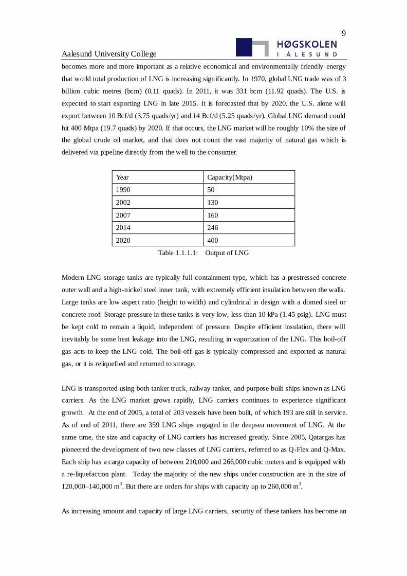
that world total production of LNG is increasing significantly. In 1970, global LNG trade was of 3
billion cubic metres (bcm) (0.11 quads). In 2011, it was 331 bcm (11.92 quads). The U.S. is
expected to start exporting LNG in late 2015. It is forecasted that by 2020, the U.S. alone will
export between 10 Bcf/d (3.75 quads/yr) and 14 Bcf/d (5.25 quads/yr). Global LNG demand could
hit 400 Mtpa (19.7 quads) by 2020. If that occurs, the LNG market will be roughly 10% the size of
the global crude oil market, and that does not count the vast majority of natural gas which is
delivered via pipeline directly from the well to the consumer.
Year Capacity(Mtpa)
1990 50
2002 130
2007 160
2014 246
2020 400
Table 1.1.1.1: Output of LNG
Modern LNG storage tanks are typically full containment type, which has a prestressed concrete
outer wall and a high-nickel steel inner tank, with extremely efficient insulation between the walls.
Large tanks are low aspect ratio (height to width) and cylindrical in design with a domed steel or
concrete roof. Storage pressure in these tanks is very low, less than 10 kPa (1.45 psig). LNG must
be kept cold to remain a liquid, independent of pressure. Despite efficient insulation, there will
inevitably be some heat leakage into the LNG, resulting in vaporization of the LNG. This boil-off
gas acts to keep the LNG cold. The boil-off gas is typically compressed and exported as natural
gas, or it is reliquefied and returned to storage.
LNG is transported using both tanker truck, railway tanker, and purpose built ships known as LNG
carriers. As the LNG market grows rapidly, LNG carriers continues to experience signif icant
growth. At the end of 2005, a total of 203 vessels have been built, of which 193 are still in service.
As of end of 2011, there are 359 LNG ships engaged in the deepsea movement of LNG. At the
same time, the size and capacity of LNG carriers has increased greatly. Since 2005, Qatargas has
pioneered the development of two new classes of LNG carriers, referred to as Q-Flex and Q-Max.
Each ship has a cargo capacity of between 210,000 and 266,000 cubic meters and is equipped with
a re-liquefaction plant. Today the majority of the new ships under construction are in the size of
120,000–140,000 m3. But there are orders for ships with capacity up to 260,000 m
3.
As increasing amount and capacity of large LNG carriers, security of these tankers has become an
10
Aalesund University College
essential issue in maritime transportation. During their voyage, inevitably they will encounter the
bad weather with large wave. Thus they have not only the wave load but also the sloshing load of
the tank due to the large ship motion if the tank is partly filled. When the frequency of ship motion
in wave is close to the natural frequency of LNG in the tank, there will be severe sloshing motion
and cause significant impact force to tank structure. This short-time, violent force is easy to
damage the tank structure. In history, accidents of the tanker that instability or local structural
damage due to sloshing motion have occurred several times. Not only the leak of the liquid that
contain chemicals will pollute the ocean but also the inflammable may cause severe explosion or
fire disaster, which are the serious threats to life and properties.
Considering this, sloshing has been an important design criterion for liquid tankers(oil, LNG, and
so on). It is essential for the security assessments for the tankers on voyage. Besides, study of the
sloshing load is also one part of the Ship Structural Mechanics.
1.1.2.Purpose
In 21 century, natural gas has become an indispensable part of the world energy consume. Firstly,
it's essential to find the replacement of the crude oil since the rapid consume of this nonrenewable
energy. Considering the chemical properties of natural gas, it could be used as fuel in a large
amount of fields such as industry, road vehicle and daily life. Secondly, natural gas is a clean and
environmentally friendly energy compared to crude oil. It contains almost no sulfur, dust and other
harmful substances. It produce relatively little carbon dioxide than other fossil fuels, which
resulting in lower greenhouse during combustion that can fundamentally improve the quality of
environment. What's more, natural gas is non-toxic and easy to distribute. Its density is less than
the air that reduce the risk of accumulation to the explosive gas. Thus the natural gas is a relatively
safe and reliable energy.
The transportation of the natural gas is a technical project. Nowadays, maritime transportation
plays an important role for transporting liquefied natural gas. LNG carrier, as the tanker for
transport LNG on the sea, have to be designed and built specifically to overcome several technical
difficulties. For example the extremely low temperature and the topic of this master
thesis--sloshing load. Currently only a few countries such as United States, China, Japan, Korea
and some Europe countries are capable of building this kind of tanker. Considering the situation of
global LNG utilization, LNG carrier will become more and more competitive in the future.
However, academic and technical issues of LNG carrier are still not perfect and researches of
these issues are valuable.
11
Aalesund University College
Among these issues, sloshing motion and sloshing loads of LNG tank as well as methods for the
prevention of tremendous impact loads are the crucial issues that need further researching. In the
field of shipbuilding of LNG carrier , analysis and researches about sloshing are not much. Thus,
this research and master thesis is carried out in order to provide technical and academic reference
related to ship motion and ship structural mechanics for the build of LNG carrier.
1.2.Sloshing
In fluid dynamics, sloshing refers to the movement of two or more immiscible fluids(generally
liquid and gas) inside another object (which is, typically, also undergoing motion). Feather of the
sloshing is that the liquid must have a movable free surface. Sloshing is a common phenomenon
of fluid motion and always occurs in partly filled tank. Such as propellant slosh in spacecraft tanks
and rockets (especially upper stages), cargo slosh in ships and trucks transporting liquids (for
example oil, gasoline and LNG), the stored liquid s losh in nuclear reactors and reservoirs tanks in
earthquake, wave motion near the port, and so on. Sloshing motion is a complicated fluid
movement. When frequency of external excitation is close to natural frequency of liquid in partly
filled tank or amplitude of excitation is very large, sloshing motion in the tank will be severe. Thus
the impact force to the side or ceiling of tank will be signif icantly strong and destroy the structure.
Sloshing can cause serious problems so that necessary prevention is essential. For example, in
aerospace field, sloshing of the liquid for attitude adjustment of the Earth Satellite may cause
instability of it without careful treatment. In working process of launch vehicle, sloshing of liquid
propellant in fuel tank will disturb the normal operation of vehicle control system that generate
instable propulsion power. In earthquake, sloshing motion in oil tank will bring about large
hydrodynamic pressure and impact loads, which might destroy the structure of tank. Seriously, fire
disaster or wide-area environmental pollution will occur, which are extremely dangerous,
especially for nuclear reactor. On sea, ship motion of tankers in waves might cause sloshing in
partly filled tank, which will lead to instability of tankers. Severe sloshing motion may produce
large impact force to tank wall and structure and destroy them. The leakage of oil or LNG is a big
threaten to environment and personal safety. However, if sloshing is made reasonable used, it will
become advantageous to us. Such as the roll-reduction tank that use the force and moment
provided by sloshing motion in the tank to reduce the ship motion in wave. In skyscrapers there
are always boxes whose natural frequency are different from the building to reduce amplitude of
damping. From the example mentioned above, in order to control or make use of sloshing motion,
study and research of mechanism of sloshing is necessary.
Besides, sloshing is a specific movement of fluid that research of it has mathematical and physical
12
Aalesund University College
sense. Sloshing has not only feathers of regular movement of free surface but also strong
interaction between liquid and structure that restrict the liquid motion. In addition, Sloshing
motion is a highly nonlinear fluid movement. Here nonlinear means large motion of free surface,
fast change of wet boundary and fluid-structure coupling. Because of its complexity, so far
theoretical analysis of sloshing are not perfect. Nowadays sloshing is still the hot topic in
aerospace and marine fields. Thus experimental test and numerical simulation of sloshing are also
necessary and excellent methods for sloshing researches and valuable to supplement theoretical
analys is.
1.3.Previous Research
The research of sloshing has a long history and continues to attract attention because of its
importance in application. After several decades' developments, a large amount of achievements of
sloshing researches has been reached and several effective methods for researching has been built.
However, because of its highly nonlinear feather, solving of the sloshing is still a big challenge
and a lot of work is still required. Typically, there are mainly three methods to analyze the sloshing
phenomenon, which are theoretical analytic method, numerical method and experimental method.
1.3.1.Theoretical Analytic Method
Early achievements of sloshing researches by theoretical analytic method were always based on
linear theory that assume the small free surface oscillation. Potential theory was used to get
solution. Theoretically, there are many assumptions for potential theory. For example, irrotational
field and existing of velocity potential function. Due to these assumptions, the potential theory
model is suitable for the fluid with small viscosity, simple shape tank, high f luid level and little
impact force. In the use of potential theory, acceptable results could be obtained in small
oscillation and linear analysis. Nevertheless, when amplitude of oscillation increase, sloshing
motion becomes highly nonlinear that linear theory will never be suitable. Then alternative theory
is required to solve the sloshing problem, such as eigenfunction expansion method. When
considering the elastic deformation of tank wall, the Analytic method will become even
complicate because of the separation of variables. From the discussion above it could be
concluded that theoretical analytic method are always used for the sloshing problem with simple
shape and boundary condition.
Moiseyev[1] in 1958 built a general nonlinear method based on potential flow to determine the
forced and free oscillations of the liquid in generally shaped tanks, which has been the foundation
13
Aalesund University College
of later analytical studies of sloshing. In his research, the setting oscillation frequency is close to
the lowest natural frequency of fluid motion. However, he did not carry out the derivation for
specific tank configuration detailedly.
The first comprehensive research of sloshing started in fields of aerospace and nuclear in 1966.
based on linear potential flow theory, Abramson[2] analyzed the sloshing phenomenon of fluid in
cylinder and sphere container in order to predict the influence of hydrodynamic pressure to
structure of fuel tank. Bes ides, The nonlinear theory of Moiseyev is included. Although his works
are mainly focus on aerospace field, it is the starting point of the research of sloshing.
Apart from Abramson, Faltinsen[3] in1974 carried out a nonlinear analytical method which was a
third-order theoretical sloshing model. The limitation of this method is that the result is accurate
when frequencies away from resonance, which means a calm sloshing motion. If the sloshing
becomes severe that perform highly non-linear, the result solved by the theoretical analytic
method is never accurate.
Faltinsen[4] 2000 present an analytical method of sloshing in rectangular tanks of specific water
depth. The derivations are based on the Bateman-Luke variational principle and the use of the
pressure in the Lagrangian of the Hamilton principle. The solution is a series of nonlinear ordinary
differential equations in time the generalized coordinates of the free surface elevation. The results
applies to any tank configurations when tank walls are vertical near mean free surface. This
method is validated for forced motion.
Although theoretical analytical method is the perfect way for building mathematical model and
convenient to apply in practice, for sloshing problem only models with simple shape and boundary
or simplif ied models can be solved and analytical solutions can be obtained. Normally, when there
are inner structures in tank such as bulkhead, or fluid liquid with high viscosity, the mechanism of
wave breaking, as well as the elastic deformation of tank wall, influence of viscosity to the
movement should be considered and more complex N-S equations should be applied. For this
situation, another two methods--numerical and experimental methods are more suitable for
solutions.
1.3.2. Numerical Method
The development of high speed computer, the graduate maturation of technique of computational
fluid dynamic have allowed a new, and powerful approach to analyzing sloshing--numerical
14
Aalesund University College
methods. When the sloshing motion is severe with large amplitude, movement of free surface is
highly nonlinear. Therefore, in numerical method, one of the most difficult issues is the method of
confirming this free surface movement. All these approaches are base on it. According to the
description of fluid movement, there are Lagrangian, Euler and arbitrary Lagrangian approaches.
According to way of discrete the fluid equations there are Finite Difference Method(FDM), Finite
Element Method(FEM), Boundary Element Method(BEM) and Finite Volume Method(FVM). For
free surface movement tracking methods there are Moving Grid Method, Elevation Method,
Volume of Fluid(VOF), Marker and Cell(MAC), Level-set and Smoothed Particle
Hydrodynamics(SPH). Nowadays, several commercial code such as ADINA, ANSIS, FLUENT,
STAR-CCM+, SPH-FLOW are based on these methods. All these method are focus on different
parts and for specific questions, one or several method could be combined to get approach to
optimal solution. In the following, these methods are introduced in detail.
(a)Finite Difference Method(FDM) and Finite Volume Method(FVM)
In mathematics, Finite difference method (FDM) is numerical method for solving differential
equations by approximating them with difference equations, in which finite differences
approximate the derivatives. FDMs are thus discretization methods. In fluid mechanics, this
method means the flow field is divided by structural grids made up with a finite number of fix
discrete points. In each grid velocity and pressure is defined and the equations is solved
differentially using an Eulerian method. The results is a system of algebraic equations for the
unknown flow variables.
The Finite Volume Method divided the whole domain into a finite number of discrete adjacent
control volume. FVM will calculate the values of the variables averaged belong to the volume.
There are two steps of discretizing the governing equations. Firstly, each control volume is
integrated. Then the resulted cell boundary values are approximated. Apart from FDM, FVM does
not required a structural mesh. In fact, there is no strict distinction between FDM and FVM. Thus
a method described as a FVM may use control volume method.
For dealing with free surface flow by FDM or FVM, some kinds of volume tracing methods are
always applied. Some basic feathers are carried out by Rider and Kothe[5] in 1998. When dealing
with the sloshing motion with free surface, the two most wildly used volume tracing methods are
Marker and Cell(MAC) and Volume of Fluid(VOF).
An early method of surface tracing is the Marker and Cell method. The MAC method is
commonly used in computer graphics to discretize functions for fluid and other simulations . It was
developed by Harlow and Welch[6] at the Los Alamos National Laboratory in 1965. This method
15
Aalesund University College
divides the flow domain into cells and sets a series of particles without mass that move with the
local flow. A cell without particles represent the domain without fluid. A cell with particles near
the empty cells means the free surface. According to these particles, interface of different
materials(including free surface) could be represent obviously. This method is always applied for
solving incompressible and viscous flow with free surface, or even wave breaking phenomenon.
Defeat of it is that large computational memory and sophisticated surface treatment technology are
required.
Feng[7] in 1973 used a three-dimensional version of the marker and cell method (MAC) to study
sloshing in a rectangular tank. This method consumes large amount of computer memory and CPU
time and the results reported indicate the presence of instability. After several decades effort, this
method has been constantly improved and gradually applied in all kinds of flow simulation with
free surface.
Another highly used method of volume tracing is the Volume of Fluid Method(VOF), which is
given by Hirt and Nichols[8] in 1981 to simulate the flow with free surface. VOF comes from
MAC and has all the basic feathers of volume tracing methods. In VOF a volume fraction is used
to represent the volume discrete data so that it provides more information than the MAC method.
The so-called fraction function C is a scalar function, defined as the integral of a fluid's
characteristic function in the control volume, namely the volume of a computational grid cell. The
volume fraction of each fluid is tracked through every cell in the computational grid, while all
fluids share a single set of momentum equations. When a cell is empty with no traced fluid inside,
the value of C is zero; when the cell is full, C=1; and when there is a fluid interface in the cell, 0 <
C < 1. C is a discontinuous function, its value jumps from 0 to 1 when the argument moves into
interior of traced phase. The normal direction of the fluid interface is found where the value of C
changes most rapidly. With this method, the free-surface is not defined sharply, instead it is
distributed over the height of a cell. Thus, in order to attain accurate results, local grid refinements
have to be done. The refinement criterion is simple, cells with 0<C<1 have to be refined.
For VOF method, a excellent reconstruction algorism is the key for success. From the time VOF
method published, significant improvement has been made by different researchers. By using
commercial code--FLOW-3D developed by Flow Science, Solaas[9] has made a research related
to sloshing motion. This software combine finite difference scheme for solving Navier-Stokes
equations with the VOF approach. The influence of the choice of numerical parameters to the
results and the finding that lack of conservation of fluid mass will cause unphysical sloshing
behavior was carried out.
Rudmen[10] compared the well-known method with a new technique. Besides, he made a
16
Aalesund University College
conclusion that Youngs(1982) has a better VOF algorithm than that of Hirt and Nichols published
in 1981.
Van Daalen et al.[11] carried out numerical simulations of the water movement inside a anti-roll
tank with free surface based on VOF method. He measured and calculated roll moment amplitudes
and found that phases are in nice agreement for different combinations of motion and tank
parameters. In his researches the filling level represents the shallow water situation.
Kim[12] has carried out a solver to Navier-Stokes equations based on the SOLA scheme. He
assumed the free surface as a single-valued function and present a special treatment of impacts
between free surface and tank ceiling. A buffer zone is applied that a mixed boundary condition of
rigid wall and free surface is imposed before impacts. The impact pressure calculated depends on
size of zone but a time-averaged technique is used to reduce the dependency. The calculated
impact pressure and integral flow are agree well with experimental results and other calculated
results.
Celebi [13] made a research about the sloshing of a two dimensional rectangular tank. The
nonlinear sloshing motion was a forced motion perpendicular to a curve. Baffle was also applied
in the research. He made the assumption of contiguous and isotropic flow with viscosity and finite
compressibility. VOF method is used to trace the free surface and Navier-Stokes equations with
initial variations is solved by FDM. In each step, function of volume fraction and position of free
surface is delivered by Donor - acceptor approach. The results also coincide the experimental
results and other calculated results
Akyildiz[14] studied the pressure distribution and three dimens ional effects of a horizontal moved
rectangular tank. The study is also based on VOF method. In the study, complete N-S equations
are solved with initial variations and the results are averaged in each time step. The results are
agree well with the experiment both for impact sloshing load and sustained loading.
Liu[15] had applied a new tank model to study the 3-D nonlinear sloshing motion with breaking
free surface. The numerical simulation use LES method the SGS closed model to simulate
turbulent effect. Besides, pressure Poisson equation is solved by Two-step projection method and
Bi-CGSTAB technology. In addition, Second-order accurate VOF method is used to trace the
breaking free surface motion. And partial averaged N-S equation in non-inertial reference system
with 6 DoF is solved. The results shows that for small oscillation, numerical solution is agree well
with the analytical solution. When oscillation amplitude increase signif icantly, numerical solution
is not so agree with analytical solution but experimental results.
17
Aalesund University College
(b) Finite Element Method(FEM)
Finite Element Method uses a different discretization process than FDM. In mathematics, the
Finite Element Method is a numerical technique for finding approximate solutions to boundary
value problems for partial differential equations. It uses subdivision of a whole problem domain
into simpler parts, called f inite elements, and variational methods from the calculus of variations
to solve the problem by minimizing an associated error function. Analogous to the idea that
connecting many tiny straight lines can approximate a larger circle, FEM encompasses methods
for connecting many simple element equations over many small subdomains, named finite
elements, to approximate a more complex equation over a larger domain. Initially, FEM was used
in solid mechanics field to solve the structural and small deformational problem. Now in fluid
dynamics this method is also applied and there are researches that use the Lagrangian-Euler ian
FEM method to solve the sloshing problem in elastic tank. However, for fluid dynamic problems,
FEM is not so widely used as FDM for three reason: In the application of solid mechanics,
operators are always symmetric while in fluid dynamics are not, thus new technology is required
to solve this; Accuracy of FEM is higher than FDM when solving high-level element but more
computational memory and time is needed so FDM is always chose; FEM method is hard to solve
the problem like incompressible flow.
Apart from FDM and FVM, fro FEM a Lagrangian approach is used and the node points and
elements will move with the flow. This may be a big challenge for large deformation of domain
since the element are deformed causing low accuracy. Possible solution for this may be a adaptive
regridding of the domain. Ramaswamy and Kaw Ahara[16] dealt with the large free surface
motion by using a arbitrary Lagrangian-Eulerian kinematic description of the domain, which is
called ALE method. The node points can be placed independently of the flow motion that they can
flow with the fluid of Lagrangian computation, or they can fixed for Eulerian computation, or they
can move in an arbitrary way to give contiguous rezoning.
Okamato and Kaw Ahara[17] carried out a Lagrangian finite element to solve N-S equations. They
built a 2-D rectangular tank and calculated the free surface elevation. Compared with video
snapshots from experiments with the similar tank excited in horizontal direction, a acceptable
agreement is reported. Besides, numerical calculations without experimental comparison and
convergence research of element size and time step are given for a multi-slope wall.
Mashayek and Ashgriz[18] developed a numerical technique to simulate the free surface flow and
interfaces. In this technique a FEM is applied to calculate field variables and a VOF is applied to
deal with the f luid interface and N-S equations govern the flow. They found that this combined
method can handle large surface deformations if boundary treatment is accurate. This technique
18
Aalesund University College
was then applied in several related researched by them.
Wu et al.[19] simulated the sloshing motion in 2-D and 3-D tanks using FEM based on fully
nonlinear wave potential theory. A good agreement between calculated results and published 2-D
data validates the used method and results. In the simulation, not only normal standing waves but
also traveling waves and swell phenomenon could be found. Furthermore, more results are given
for a rectangular tank undergoing translatory motion in several direction.
(c) Boundary Element Method(BEM) and other method
Boundary element method are based on potential flow assumptions that the flow is assumed
incompressible and irrotational as well as the negligence of viscosity. Greens second function is
applied and the flow is governed by Laplace equation. Compared with FDM and FEM, the main
feather of BEM is that only equations on the boundary need to be solved so that a simplif ication of
the problem from 3-D to 2-D and 2-D to 1-D will reduce the unknown significantly. This method
was present by C.A.Brebbia[20] in Southampton in 1970s and due to its imperfection, much
improvements is required before widely used.
Other methods contain Smoothed Particle Hydrodynamics(SPH) method. It is a computational
method used for simulating fluid f lows. It was developed by Gingold and Monaghan [21] initially
for astrophysical problems. This method works through dividing fluid into a set of discrete
elements, referred to as particles. These particles have a spatial distance known as "the smoothing
length" over which their properties are "smoothed" by a kernel function. This means that the
physical quantity of any particle can be obtained by summing the relevant properties of all the
particles which lie within the range of the kernel.
1.3.3.Experimental Method
Although all kinds of numerical methods is carried out and could be successfully applied in all
fields of fluid dynamics, they still have their own limitation. For example, the feather of
approximate calculation of numerical method requires a validation from real. Therefore,
experimental method is still an important approach to study the sloshing phenomenon and validate
the numerical results as well as providing the empirical correction factor for practical application.
Researchers have investigated sloshing of liquid experimentally in the last decades. The special
NASA monograph edited by Abramson(1966) represented the sloshing problems encountered in
aerospace vehicles. Besides, Abramson et al(1974) made a great contribution to the experimental
19
Aalesund University College
approach to analyze the sloshing impact load in LNG tank, which was a good supplement of
numerical method.
Akyildiza[22] present an experimental study of sloshing motion in 3-D rectangular tank. Variable
parameters such as excitation frequency, liquid filling and baffle are considered and test. In the
experiment pressure distribution and three dimensional effects is researched. The systematic
variation of parameters could provide of sensibility of sloshing system. Some conclusions such as
the damping of sloshing depend on liquid filling, viscosity and size of tank.
Nasar[23] made a experimental study of liquid sloshing dynamics in a barge carrying tank. Ship
motion of barge is the combination of surge, sway and pitch. Liquid fillings of 25%, 50% and 75%
is considered. Excitation wave height and frequency is also included. The sloshing motion is
observed and recorded. Besides, the response of barge is also researched.
Recently, Panigrahy[24] has made a experimental research of the sloshing motion in a cube tank.
In the experimental pressure distribution and force of tank wall and ceiling is considered.
Influence of baffle is also tested.
1.3.4.Fluid Structure Interaction
All of the tank of sloshing motion discussed above is the rigid structure, which is not in practice.
In real tank structure elasticity should be considered. For LNG carrier, in order to keep low
temperature and hydrodynamic pressure, its insulation shell is made up of several metals and
composite materials. If it is assumed to be a rigid structure, deformation and strain encountered
sloshing load will be ignored. What's more, interaction between elastic structure and inner flow
may even important that will be ignored. This interaction will change the impact force and
distributed force significantly, especially when duration time of impact force is close to the period
of elastic structure. This is so-called hydroelastic ity. Due to the limitation of condition and time, in
this paper all the tanks are still rigid structure and hydroelasticity is not considered. However,
further work is required related hydroelasticity to validate the research and improve the results.
1.4.Summery of the Thesis
From the historical researches mentioned above, it could be seen all the methods(theoretical
analytical, numerical and experimental) is used in the study of sloshing motion. For numerical
method, both the VOF and MAC approaches is widely applied. However, for VOF method, the
model of the tank is usually two dimensional or three dimensional regular rectangular tank.
20
Aalesund University College
Besides, simulation tools are some early software or codes. In addition, little comparison
between two dimensional and three dimensional results is carried out to test three dimensional
effects.
With the development of technology for LNG carrier, the requirements of the structural strength is
higher and higher. More and more factors and situation should be considered in the service of the
LNG carrier. Among these factors, sloshing load has become a important design parameters of
fatigue consideration. Therefore, in this thesis, the newest CFD codes STAR-CCM+ is applied to
simulate the sloshing motion and calculate sloshing liquid. Both two dimensional and three
dimensional cases of prismatic tanks are simulated and compared. Finally, sloshing cylindrical
tank in longitudinal direction is carried out for the important types of tank.
Detailed arrangement of the thesis is as follow: First and second chapter is the introduction of the
topic and type of LNG tank, respectively. In chapter 3, theoretical analysis of the model and
mathematical formula are given. And some basic introduction about STAR-CCM+ is present.In
chapter 4, basic setting of the model is introduced; the model is simulated and validated by a
published experimental results; Natural frequency of the tank is calculated by empirical formula
and validated by the numerical methods. Other effects of the model is also carried out. In chapter 5,
the LNG tanks are built. Both two dimensional and three dimensional cases are included. Both
prismatic tank and cylindrical tank are simulated. Finally, in chapter 6, summary of the work and
main conclusion of this thesis are given.
21
Aalesund University College
2.Overview of LNG Carrier and Tank Sloshing
2.1.LNG Carrier
LNG Carrier is the special vessel that transport LNG in -162 degree centigrade on sea. It is one
kind of high-technical, high value-added ship whose building technique represents the highest
shipbuilding level in the world. Nowadays only a few countries could build it independently.
2.1.1.Brief Introduction
LNG carrier is the most important vehicle for transporting LNG. The first LNG carrier Methane
Pioneer whose dwt was 5034 tons, refitted from a general cargo ship, left the Calcasieu River on
the Louisiana Gulf coast on 25 January 1959. It sailed to the UK where the cargo was delivered,
which carried the world's first ocean cargo of LNG.
Generally, dwt of these kinds of ship is between 1.2~1.5 million cubic meters. Service speeds are
always between 17~20 knots while for large oil tanker 14~16 knots are the most. Life of this kind
of vessel is always 40~60 years. Tanks in LNG carrier are independent structures and materials of
tank should maintain ductility in low temperature of -162 centigrade degree. In transporting, tanks
are always not fully filled, usually 96%~97% of the whole volume to remain redundancy of the
gasification of natural gas. Usually draught for large LNG carrier is around 11m while super
structure above the water place is 15m. Thus LNG carrier may even look larger than some VLCC.
When the volume of LNG carrier need to increase, usually length of the vessel in increased.
On voyage of LNG carrier, temperature difference between inside and outside of tank would cause
heat transfer and gasification of LNG. Therefore, in early design of LNG carrier, the boil-off gas is
used as the fuel of vessel. However, according to ICG code, other fuel such as the diesel is
required as the supplemental fuel. So, there are some Boil-off natural gas remain, especially in
return, for the fuel of engine and maintaining temperature of tank.
Considering the feathers of LNG, design of LNG carrier should contain the materials for the tank
that could encountered the extremely low temperature, the handling of volatile and f lammable
feathers and ability to store the cargo with low proportion. For international standard, tank
material used in -162o
C should contains 9% nickel steel, austenitic stainless steel, 36% nickel
steel and aluminium alloy. For the leakage of LNG, 15 days should be ensured to prevent it.
Because no matter how far the vessel sails, it could return to the yard within 15 days. Thus the
22
Aalesund University College
tank are always bilayer structure to prevent the leakage. In addition, the tank should maintain the
low temperature. Usually the requirement is that daily evaporate percentage is lower than 0.15%.
2.1.2.Tank Types
During the development of LNG carrier there are different tank types. The main purpose of the
cargo storage system is to keep the LNG cargo below its boiling point and maintaining the
reasonable insulation. According to this it's important to select the suitable storage system. Besides
the tank’s capability to withstand loads such as sloshing loads should also be take into
consideration. Generally, the tank designs can be divided into two main categories : the membrane
tanks and the independent tanks. The membrane category includes two designed tank types used
for LNG--the membrane tanks and the semi-membrane tanks. Although the tank types have
different designs, some feathered elements are the same in all tanks. For example, the double
bottom and the secondary barrier are very important for the prevention of leakages of the LNG to
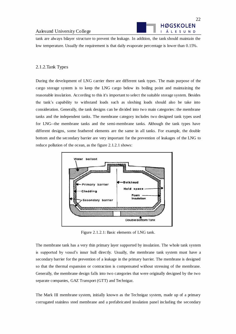
reduce pollution of the ocean, as the figure 2.1.2.1 shows:
Figure 2.1.2.1: Basic elements of LNG tank.
The membrane tank has a very thin primary layer supported by insulation. The whole tank system
is supported by vessel’s inner hull directly. Usually, the membrane tank system must have a
secondary barrier for the prevention of a leakage in the primary barrier. The membrane is designed
so that the thermal expansion or contraction is compensated without stressing of the membrane.
Generally, the membrane design falls into two categories that were originally des igned by the two
separate companies, GAZ Transport (GTT) and Technigaz.
The Mark III membrane system, initially known as the Technigaz system, made up of a primary
corrugated stainless steel membrane and a prefabricated insulation panel including the secondary
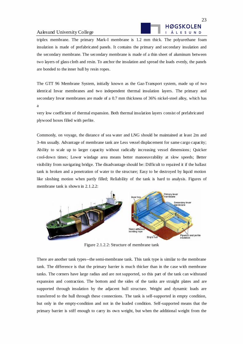
23
Aalesund University College
triplex membrane. The primary Mark-I membrane is 1.2 mm thick. The polyurethane foam
insulation is made of prefabricated panels. It contains the primary and secondary insulation and
the secondary membrane. The secondary membrane is made of a thin sheet of aluminum between
two layers of glass cloth and resin. To anchor the insulation and spread the loads evenly, the panels
are bonded to the inner hull by resin ropes.
The GTT 96 Membrane System, initially known as the Gaz-Transport system, made up of two
identical Invar membranes and two independent thermal insulation layers. The primary and
secondary Invar membranes are made of a 0.7 mm thickness of 36% nickel-steel alloy, which has
a
very low coefficient of thermal expansion. Both thermal insulation layers consist of prefabricated
plywood boxes filled with perlite.
Commonly, on voyage, the distance of sea water and LNG should be maintained at least 2m and
3-4m usually. Advantage of membrane tank are Less vessel displacement for same cargo capacity;
Ability to scale up to larger capacity without radically increasing vessel dimensions ; Quicker
cool-down times; Lower windage area means better manoeuvrability at slow speeds; Better
visibility from navigating bridge. The disadvantage should be: Difficult to repaired it if the ballast
tank is broken and a penetration of water to the structure; Easy to be destroyed by liquid motion
like sloshing motion when partly filled; Reliability of the tank is hard to analysis. Figures of
membrane tank is shown in 2.1.2.2:
Figure 2.1.2.2: Structure of membrane tank
There are another tank types--the semi-membrane tank. This tank type is similar to the membrane
tank. The difference is that the primary barrier is much thicker than in the case with membrane
tanks. The corners have large radius and are not supported, so this part of the tank can withstand
expansion and contraction. The bottom and the sides of the tanks are straight plates and are
supported through insulation by the adjacent hull structure. Weight and dynamic loads are
transferred to the hull through these connections. The tank is self-supported in empty condition,
but only in the empty-condition and not in the loaded condition. Self-supported means that the
primary barrier is stiff enough to carry its own weight, but when the additional weight from the
24
Aalesund University College
gas puts pressure on the tank the primary barrier is not strong enough and the tank needs support
from the hull structure. In other words, the tank is not designed to be placed on the deck, it must
be inside the vessel.
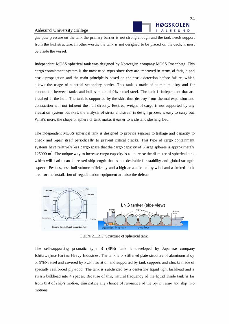
Independent MOSS spherical tank was designed by Norwegian company MOSS Rosenberg. This
cargo containment system is the most used types since they are improved in terms of fatigue and
crack propagation and the main principle is based on the crack detection before failure, which
allows the usage of a partial secondary barrier. This tank is made of aluminum alloy and for
connection between tanks and hull is made of 9% nickel steel. The tank is independent that are
installed in the hull. The tank is supported by the skirt thus destroy from thermal expansion and
contraction will not influent the hull directly. Besides, weight of cargo is not supported by any
insulation system but skirt, the analysis of stress and strain in design process is easy to carry out.
What's more, the shape of sphere of tank makes it easier to withstand sloshing load.
The independent MOSS spherical tank is designed to provide sensors to leakage and capacity to
check and repair itself periodically to prevent critical cracks. This type of cargo containment
systems have relatively less cargo space that the cargo capacity of 5 large spheres is approximately
125000 m3. The unique way to increase cargo capacity is to increase the diameter of spherical tank,
which will lead to an increased ship length that is not desirable for stability and global strength
aspects. Besides, less hull volume efficiency and a high area affected by wind and a limited deck
area for the installation of regasification equipment are also the defeats.
Figure 2.1.2.3: Structure of spherical tank.
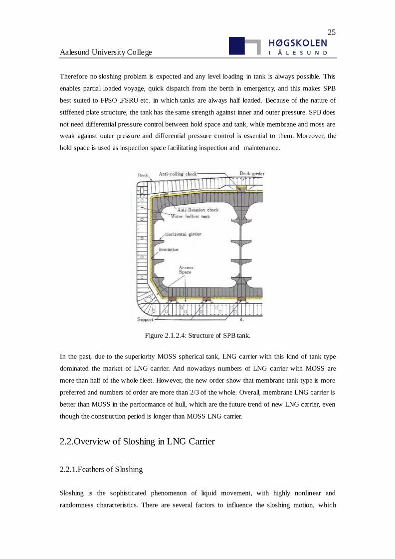
The self-supporting prismatic type B (SPB) tank is developed by Japanese company
Ishikawajima-Harima Heavy Industries. The tank is of stiffened plate structure of aluminum alloy
or 9%Ni steel and covered by PUF insulation and supported by tank supports and chocks made of
specially reinforced plywood. The tank is subdivided by a centerline liquid tight bulkhead and a
swash bulkhead into 4 spaces. Because of this, natural frequency of the liquid inside tank is far
from that of ship’s motion, eliminating any chance of resonance of the liquid cargo and ship two
motions.
25
Aalesund University College
Therefore no sloshing problem is expected and any level loading in tank is always possible. This
enables partial loaded voyage, quick dispatch from the berth in emergency, and this makes SPB
best suited to FPSO ,FSRU etc. in which tanks are always half loaded. Because of the nature of
stiffened plate structure, the tank has the same strength against inner and outer pressure. SPB does
not need differential pressure control between hold space and tank, while membrane and moss are
weak against outer pressure and differential pressure control is essential to them. Moreover, the
hold space is used as inspection space facilitating inspection and maintenance.
Figure 2.1.2.4: Structure of SPB tank.
In the past, due to the superiority MOSS spherical tank, LNG carrier with this kind of tank type
dominated the market of LNG carrier. And nowadays numbers of LNG carrier with MOSS are
more than half of the whole fleet. However, the new order show that membrane tank type is more
preferred and numbers of order are more than 2/3 of the whole. Overall, membrane LNG carrier is
better than MOSS in the performance of hull, which are the future trend of new LNG carrier, even
though the construction period is longer than MOSS LNG carrier.
2.2.Overview of Sloshing in LNG Carrier
2.2.1.Feathers of Sloshing
Sloshing is the sophisticated phenomenon of liquid movement, with highly nonlinear and
randomness characteristics. There are several factors to influence the sloshing motion, which
26
Aalesund University College
could be summarized as follow: frequency and amplitude of ship motion which depend on the
loading condition of ship, wave behavior in the sailing area, service speed of ship, and so on;
Natural frequency of the sloshing liquid that depends on the geometry of tank, filling lever and
nonlinear effects of large motion; Damping effect of inner structure that may reduce the sloshing
motion to some degree; viscosity of the liquid while there are no systematic research shows this
yet; Cushion effect of the gas.
Generally, sloshing motion has several forms. Always the sloshing motion observed in the tank is
the combination of the following form: Standing wave--always has the sloshing load to tank
ceiling; Travelling wave--always has the sloshing load to tank side wall; Hydraulic jump--special
form of wave that occurs related to the frequency of tank and liquid; Swirling--the rotary motion
of liquid in the tank.
Hydrodynamic pressure produced by sloshing motion could be divided into two parts: impulse
pressure and no-impulse pressure. Impulse pressure is the quick pressure pulse when the liquid hit
the wall. Usually, it is the local high pressure during a tiny time. Impulse pressure is always
related to Travelling wave and hydraulic jump, or very large standing wave. For no-impulse
pressure, it is the slowing changed pressure that commonly seen and related more to standing
wave.
Frequency of excitation and filling level will decide the strength wave shape of sloshing motion.
Even though a small change of excitation frequency will significantly change the sloshing motion.
Amplitude of excitation not only influent the bandwidth of resonance but also the wave shape. In
addition, influence of the combination of several separated excitation depend on their own phase.
2.2.2.Prevention Methods
For LNG carrier, sloshing motion is harmful and should be prevented as much as possible. In
practice, three methods are always considered to prevent or reduced it. Firstly, partly filled tank
condition should be forbidden to the greatest extend. In fact, partly filled condition will happen
unavoidable in LNG carrier that part of the cargo should be take out in the middle of transporting.
Here a scientific plan of transporting task should be carried out. Secondly, the height of transverse
and longitudinal metacenter could be modified to change the natural frequency of hull. Thus the
resonance might be prevented even though the wave frequency is closed to the liquid in the tank.
Finally, specific bulkhead or baffle could be used to reduce the sloshing motion. It is proved that
bulkhead and baffle do reduce the sloshing motion significantly so that in today's design of liquid
tank these items has been taking into consideration.
27
Aalesund University College
3.Theoretical Analysis and Numerical Method
3.1.Theoretical Formulation
3.1.1.Governing Equations
Fluid motion is governed by conservation law of physics and basic conservation law contains
mass conservation law, momentum conservation law and energy conservation law. If the flow is in
turbulent condition, the system should respect the added turbulence transport equations.
Governing equations are the mathematical description of these conservation law.
Continuity equations, or named mass conservation equations, describes the mass conservation law
that all flow should respect. In fluid dynamics, the continuity equation states that, in any steady
state process, the rate at which mass enters a system is equal to the rate at which mass leaves the
system. The differential form of the continuity equation is:
( ) 0ut
(3.1)
where:
is the fluid density.
t is the time.
u
is the flow velocity vector field.
This equation is also one of the Euler equations in fluid dynamics. The Navier–Stokes equations
form a vector continuity equation describing the conservation of linear momentum. In addition, If
ρ is a constant, as in the case of incompressible flow, the mass continuity equation simplif ies to a
volume continuity equation:
0u
(3.2)
It means that the divergence of velocity field is zero everywhere. Physically, this is equivalent to
saying that the local volume dilation rate is zero.
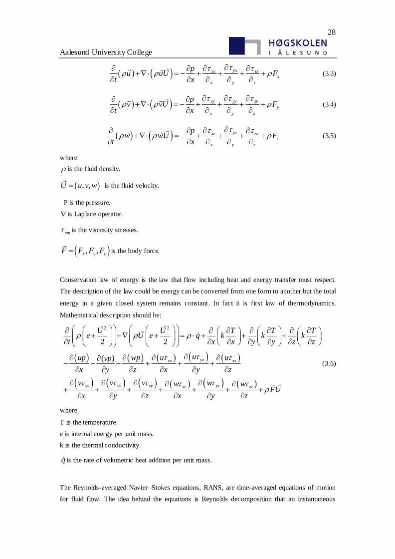
Momentum equations, or Navier-Stokes equations named after Claude-Louis Navier and George
Gabriel Stokes, describe the motion of viscous flow substances. These balance equations arise
from applying Newton's second law to fluid motion, together with the assumption that the stress in
the fluid is the sum of a diffusing viscous term proportional to the gradient of velocity and a
pressure term—hence describing viscous flow. In an inertial frame of reference, the conservation
form of the equations of continuum motion is:
28
Aalesund University College
yxxx zxx
x y z
pu uU F
t x
(3.3)
xy yy zy
y
x y z
pv vU F
t x
(3.4)
yzxz zzz
x y z
pw wU F
t x
(3.5)
where
is the fluid density.
, ,U u v w
is the fluid velocity.
P is the pressure.
is Laplace operator.
mn is the viscosity stresses.
, ,x y zF F F F
is the body force.
Conservation law of energy is the law that flow including heat and energy transfer must respect.
The description of the law could be energy can be converted from one form to another but the total
energy in a given closed system remains constant. In fact it is first law of thermodynamics.
Mathematical description should be:
2 2
2 2
( ) yxxx zx
xy yy zy yzxz zz
U U T T Te U e q k k k
t x x y y z z
uup wp u uvp
x y z x y z
v v v ww wFU
x y z x y z
(3.6)
where
T is the temperature.
e is internal energy per unit mass.
k is the thermal conductivity.
q is the rate of volumetric heat addition per unit mass.
The Reynolds-averaged Navier–Stokes equations, RANS, are time-averaged equations of motion
for fluid flow. The idea behind the equations is Reynolds decomposition that an instantaneous
29
Aalesund University College
quantity is decomposed into its time-averaged and fluctuating quantities, which is first proposed
by Osborne Reynolds. The RANS equations are primarily used to describe turbulent flows. These
equations can be used with approximations based on knowledge of the properties of flow
turbulence to give approximate time-averaged solutions to the Navier–Stokes equations. For a
stationary, incompressible Newtonian fluid, these equations can be written in Einstein notation as:
ji ij i ij i j
j j j i
uu uu F p u u
x x x x
(3.7)
where i ju u represents the fluctuating velocity field, generally referred to as the Reynolds
stress. This nonlinear Reynolds stress term requires additional modeling to close the RANS
equation for solving, and has led to the creation of many different turbulence models.
Turbulent flow is a highly nonlinear complex flow. However, it could be simulated through some
specific approached to obtain the result that agree well with the real. K-epsilon (k-ε) turbulence
model is the most common model used in Computational Fluid Dynamics (CFD) to simulate mean
flow characteristics for turbulent flow conditions. It is a two equation model which gives a general
description of turbulence by means of two transport equations (PDEs). In this paper, realizable
K-epsilon (k-ε) turbulence model is chose in STAR-CCM+ for the simulation.
There are two kinds of k-epsilon model: standard k-epsilon model and realizable k-epsilon model.
The Standard k−ɛ is a well-established model capable of resolving through the boundary layer.
The second model is Realizable 𝑘−𝜀, an improvement over the standard k−ɛ model. It is a
relatively recent development and differs from the standard k−ɛ model in two ways. The realizable
k−ɛ model contains a new formulation for the turbulent viscosity and a new transport equation for
the dissipation rate--ɛ, that is derived from an exact equation for the transport of the mean-square
vorticity fluctuation. The term "realizable" means that the model satisfies certain mathematical
constraints on the Reynolds stresses, consistent with the physics of turbulent flows.
The turbulent (or eddy) viscosity is computed by combining and as follows:
2
t
kC
(3.8)
where:
*
0
1
s
CkU
A A
*
ij ij ij ijU S S
30
Aalesund University College
2ij ij ijk kw
ij ij ijk kw
ij is the mean rate of rotation tensor viewed in a rotating reference frame with the angular
velocity k .
0 4.04, 6 cossA A
1
3
1 1cos 6 , , ,
3 2
ij jk ik i iij ji ij
i j
S S S u uW W S S S S
x xS
The turbulent kinetic energy and its rate of dissipation are obtained from the following transport
equations :
( ) ( ) tj k b M k
j j k j
kk ku P P Y S
t x x x
(3.9)
2
1 2
1 3
( ) ( ) tj
j j j
b
u C S Ct x x x k
C C P Sk
(3.10)
where:
1 max 0.43, , , 25
ij ij
kC S S S S
1 21.44, 1.9, 1.0, 1.2kC C
Besides, in these equations, Pk represents the generation of turbulence kinetic energy due to the
mean velocity gradients, calculated in same manner as standard k-epsilon model. Pb is the
generation of turbulence kinetic energy due to buoyancy, calculated in same way as standard
k-epsilon model.
3.1.2.Boundary Conditions
Boundary condition is the condition that governing equations of flow on the boundary should also
respect, which always make influence to the boundary. When the whole domain is divided into
two part and the part of fluid is represented by . which should follow the law of continuity and
momentum. Besides, varies with the time and the change of it should be obtained through free
31
Aalesund University College
surface capturing method. Due to the partly filled condition of the model, boundary conditions
should contain two parts: wall boundary conditions and free surface boundary conditions.
Wall boundary conditions includes no-slip wall and slip wall boundary condition. For no-slip wall
boundary condition:
f sd d (3.11)
For slip wall boundary condition:
f sn d n d (3.12)
where fd and
sd are the fluid velocity and structure velocity on the interface respectively, n
is
the normal vector of the interface with outer direction. In this paper, all the structures are rigid
body thus sd is equal to 0.
Similarly, dynamic condition should also be required, which means:
f sn n
(3.13)
where is the stress of fluid and structure.
Free surface is a moved boundary and obviously kinematic and dynamic conditions should be
required. For kinematic conditions, fluid particle of free surface should remain on the surface, or
normal velocity of fluid particle is agree with the surface normal velocity. Mathematical formula
for this condition is different for different free surface capturing method.
For dynamics , free surface stress condition could be represented if the surface tension is not
taking into consideration:
0n tu u
t n
(3.14)
02 nup p
n
(3.15)
where nu is the normal velocity of free surface(for fluid, outside is the positive direction) while
tu is the tangential velocity.
32
Aalesund University College
3.2.Method of Numerical Simulation of Sloshing
In this paper, commercial code STAR-CCM+ is used as the software to simulate the s loshing
motion in partly filled LNG tank. In the simulation, VOF model is selected as the approach of
volume tracing and free surface capturing.
VOF method(Volume of Fluid) is the method to simulate the f low with free surface carried out by
Hirt and Nichols. Fundamental principle of VOF method is the fraction function C of fluid and the
whole gird unit. For a gird unit, C equals to 1 means the gird is 100% fluid while 0 means
empty(gas). A value between 0~1 means the partly filled condition of fluid. There are two possible
situations for this. The one is that there are free surface in this gird. The other is that bubble is
exist in it. The gradient of C could decide the normal direction of free surface. After determining
the value and gradient of each grid, approximate position of free surface could be obtained.
Differential governing equations of C is :
0C
Cut
(3.16)
According to the continuity equations, for incompressible flow 0u , the conservative form;
0C C C C
u v wt x y z
(3.17)
which is the transport equation of the volume of fluid.
The sloshing motion in partly filled tank could be summarized as the fluid motion with free
surface. The continuity and momentum equation
0
0
uu u f
t
u
in (3.18)
where
is the constant density of liquid.
u is the velocity of liquid.
f is the volume force on the liquid.
is the tensor of deformation rate and a function of u and pressure P.
,u p pI T (3.19)
( )JT u u (3.20)
where is the dynamical viscosity of liquid.
33
Aalesund University College
For no-slip wall, u equals to 0 in . On free surface, all particles are assumed to required the
function of C x, t 0 , on moment t t , ( , ) 0C x x t t . After Taylors expansion
and conservation of the first order part, it could be obtained:
0j
j
C Cu
t x
(3.21)
Initially, the flow is stationary with standard atmospheric pressure of gas. Thus:
( ,0) 0, ( ,0) atmu x P x P (3.22)
3.3.STAR-CCM+
STAR-CCM+ is the new generation of CFD software owned by CD-adapco group. The last part of
the name – CCM – is derived from Computational Continuum Mechanics, which is the newest and
most advanced technology that combined with the modern software engineering. It has perfect
behavior and highly reliability to become an powerful tool for the thermal fluid Engineers.
STAR-CCM+ has some unique feathers. It is a powerful, all- in-one tool that combines ease of use,
all- in-one software package, automatic meshing, extensive modeling capability and powerful
post-processing. Since 2004, it has used the latest numerics and software technologies that very
large model(100M+ cells) could be designed outset to be handled. Besides, CAD and CAE is in
one package for full process integration. In addition, it has a rapid development cycle that new
release occurs every four months.
The computational continuum mechanics is the technology that models define fluid or solid
continua and the various regions of the solution domain are assigned to these continua. In terms of
simulation setup, the mesh is used only to define the topology of the problem. Topological
constructs allow communication between regions independent of the mesh (conformal or
non-conformal). Finally, it allows the user to watch the solution develop as the analysis is running
and modify the settings ―live‖.
STAR-CCM+ applies client-server approach with light weight Java front end and C++ server. The
simulation objects are created and solved on the server while the workspace views these objects
through the client. Thus the large model with high number of meshes could be solved easily with
shared CPU abilities.
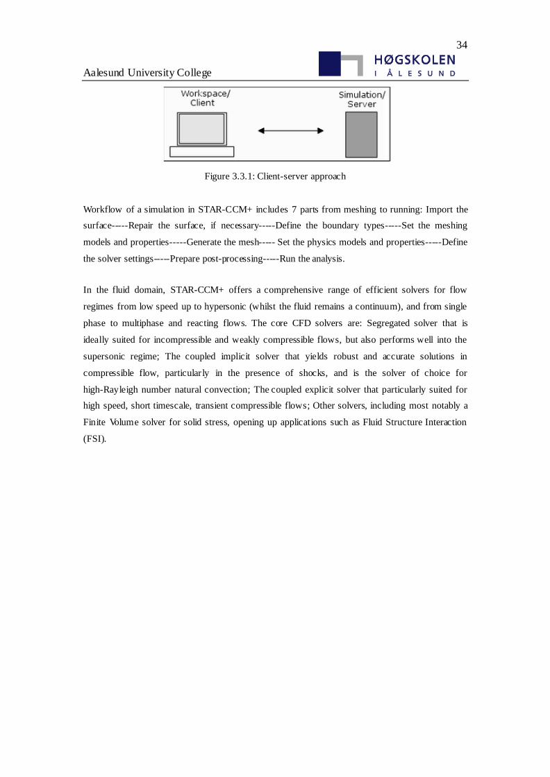
34
Aalesund University College
Figure 3.3.1: Client-server approach
Workflow of a simulation in STAR-CCM+ includes 7 parts from meshing to running: Import the
surface-----Repair the surface, if necessary-----Define the boundary types-----Set the meshing
models and properties-----Generate the mesh----- Set the physics models and properties-----Define
the solver settings-----Prepare post-processing-----Run the analysis.
In the fluid domain, STAR-CCM+ offers a comprehensive range of efficient solvers for flow
regimes from low speed up to hypersonic (whilst the fluid remains a continuum), and from single
phase to multiphase and reacting flows. The core CFD solvers are: Segregated solver that is
ideally suited for incompressible and weakly compressible flows, but also performs well into the
supersonic regime; The coupled implicit solver that yields robust and accurate solutions in
compressible flow, particularly in the presence of shocks, and is the solver of choice for
high-Rayleigh number natural convection; The coupled explicit solver that particularly suited for
high speed, short timescale, transient compressible flows; Other solvers, including most notably a
Finite Volume solver for solid stress, opening up applications such as Fluid Structure Interaction
(FSI).
35
Aalesund University College
4.Modeling and Simulation of Sloshing Tank
4.1.Model Description
For the liquid tank with the shape of rectangle or prismatic, the main direction of sloshing motion
is in direction of excitation. Besides, if all the models are calculated in three dimens ion, too much
time and memory will be consumed. Since the error is in a acceptable degree in engineering field
empirically, two dimensional models would be used and simulated in this paper. After that, three
dimensional simulation would also be simulated to compare and validate the 2-D model.
Generally, in STAR-CCM+, two main parts should be set after build or import the
surface(geometry) : Mesh model & property and physical model &property.
4.1.1.Mesh
In mesh model, Surface Remesher is selected to modify the built geometry of tank to surface that
is easier for mesh. Besides, The trimmed cell mesher provides a robust and efficient method of
producing a high-quality grid for both simple and complex mesh generation problems which are
predominantly hexahedral mesh with minimal cell skewness. Since the shape of tanks are
rectangle or prismatic, the hexahedral mesh could be considered as the shape of cell. Obviously,
they are unstructured meshes for the reason that STAR-CCM+ only provided unstructured solver.
In addition, Prism Layer Mesher is also selected as the mesh treatment near the boundary. Number
of prism layers will make a influence to the result near the boundary, which will be discussed in
the next part.
Basic size of the cells and number of prism layers will change the accuracy of the results,
especially near the boundary. Generally, two types of wall boundary condition can be considered
in numerical computation: no-slip and free-slip conditions[24].Either condition should be
combined with no-flux condition which says no water particle penetrating through the tank wall. It
is found that the no-flux condition can result in unrealistic flow, especially on the tank ceiling.
Due to the coarse resolution of numerical method, the no-flux condition tends to make fluid stay
on the tank boundary. However, necessary modification of the model could be carried out to
reduce this error. Here are two simulations of the sloshing in rectangular tanks with water, basic
size and number of prism layers for each are:
Model Basic size of cell Number of Prism layers
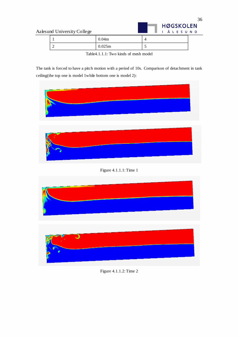
36
Aalesund University College
1 0.04m 4
2 0.025m 5
Table4.1.1.1: Two kinds of mesh model
The tank is forced to have a pitch motion with a period of 10s. Comparison of detachment in tank
ceiling(the top one is model 1while bottom one is model 2):
Figure 4.1.1.1: Time 1
Figure 4.1.1.2: Time 2
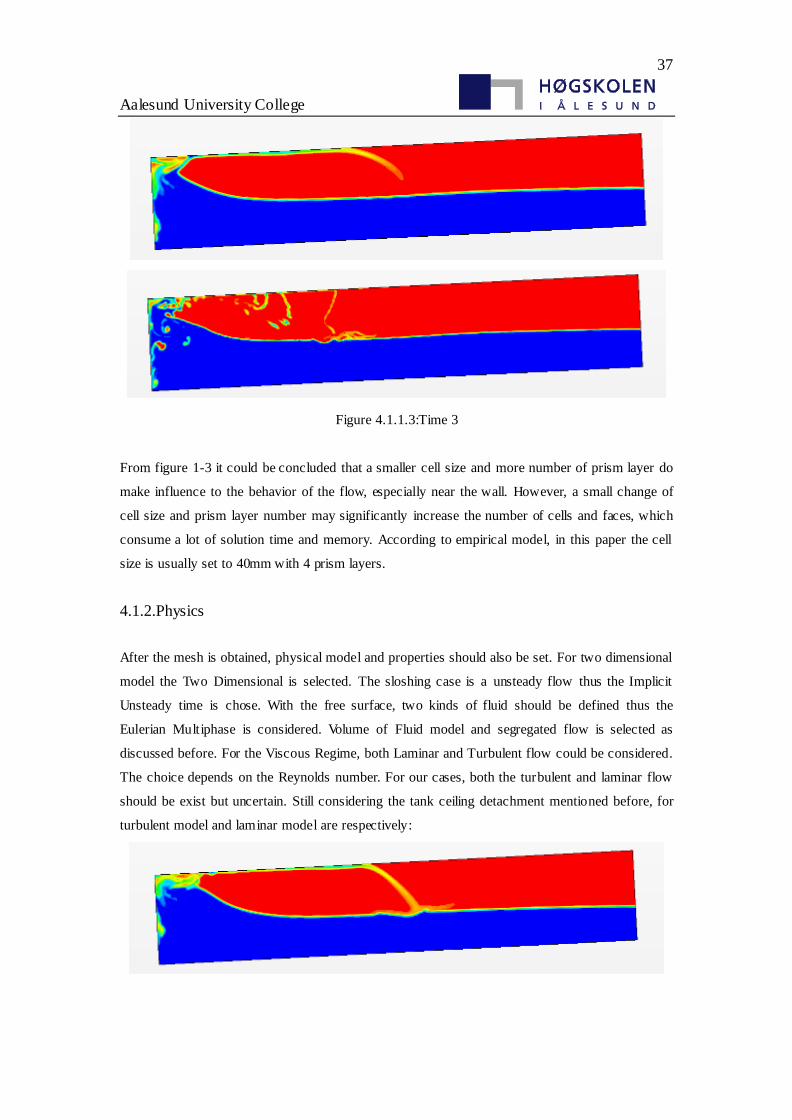
37
Aalesund University College
Figure 4.1.1.3:Time 3
From figure 1-3 it could be concluded that a smaller cell size and more number of prism layer do
make influence to the behavior of the flow, especially near the wall. However, a small change of
cell size and prism layer number may significantly increase the number of cells and faces, which
consume a lot of solution time and memory. According to empirical model, in this paper the cell
size is usually set to 40mm with 4 prism layers.
4.1.2.Physics
After the mesh is obtained, physical model and properties should also be set. For two dimensional
model the Two Dimensional is selected. The sloshing case is a unsteady flow thus the Implicit
Unsteady time is chose. With the free surface, two kinds of fluid should be defined thus the
Eulerian Multiphase is considered. Volume of Fluid model and segregated flow is selected as
discussed before. For the Viscous Regime, both Laminar and Turbulent flow could be considered.
The choice depends on the Reynolds number. For our cases, both the turbulent and laminar flow
should be exist but uncertain. Still considering the tank ceiling detachment mentioned before, for
turbulent model and laminar model are respectively:
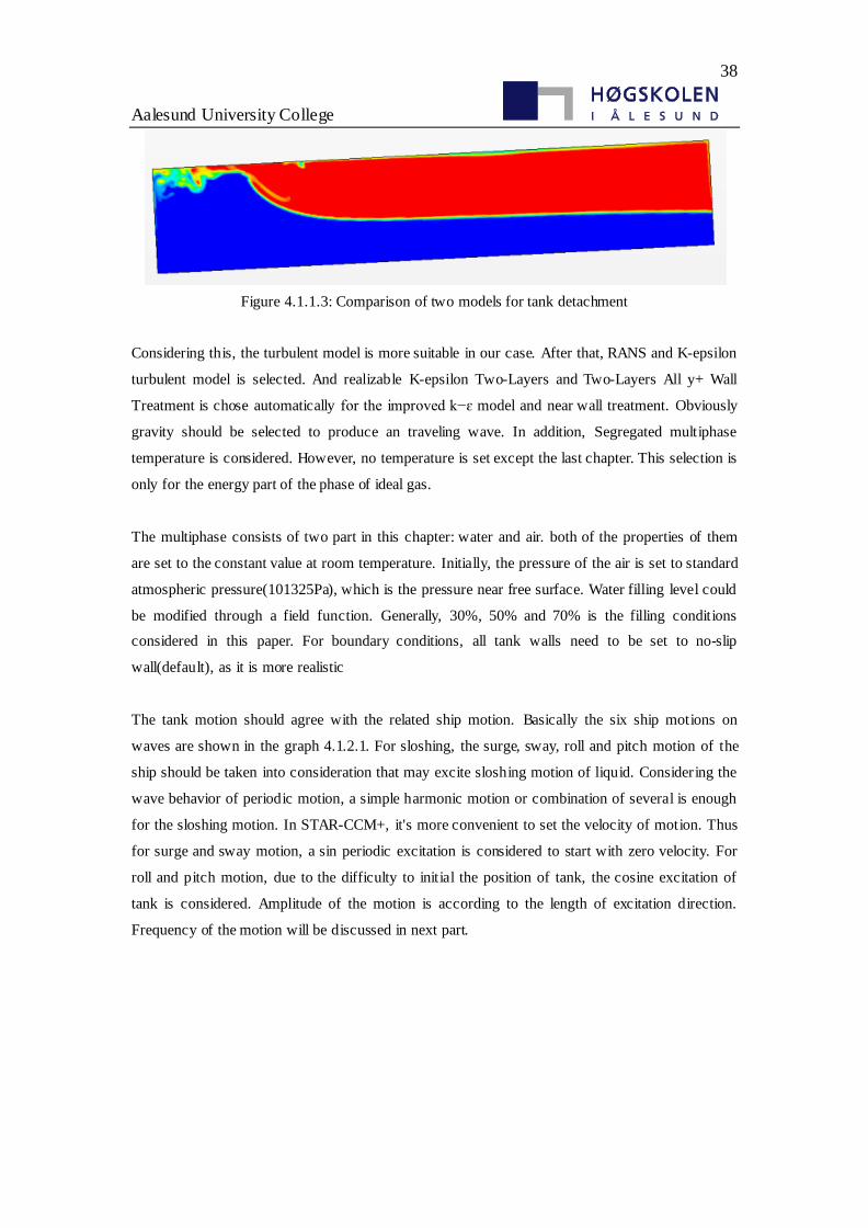
38
Aalesund University College
Figure 4.1.1.3: Comparison of two models for tank detachment
Considering this, the turbulent model is more suitable in our case. After that, RANS and K-epsilon
turbulent model is selected. And realizable K-epsilon Two-Layers and Two-Layers All y+ Wall
Treatment is chose automatically for the improved k−ɛ model and near wall treatment. Obviously
gravity should be selected to produce an traveling wave. In addition, Segregated multiphase
temperature is considered. However, no temperature is set except the last chapter. This selection is
only for the energy part of the phase of ideal gas.
The multiphase consists of two part in this chapter: water and air. both of the properties of them
are set to the constant value at room temperature. Initially, the pressure of the air is set to standard
atmospheric pressure(101325Pa), which is the pressure near free surface. Water filling level could
be modified through a field function. Generally, 30%, 50% and 70% is the filling conditions
considered in this paper. For boundary conditions, all tank walls need to be set to no-slip
wall(default), as it is more realistic
The tank motion should agree with the related ship motion. Basically the six ship motions on
waves are shown in the graph 4.1.2.1. For sloshing, the surge, sway, roll and pitch motion of the
ship should be taken into consideration that may excite sloshing motion of liquid. Considering the
wave behavior of periodic motion, a simple harmonic motion or combination of several is enough
for the sloshing motion. In STAR-CCM+, it's more convenient to set the velocity of motion. Thus
for surge and sway motion, a sin periodic excitation is considered to start with zero velocity. For
roll and pitch motion, due to the difficulty to initial the position of tank, the cosine excitation of
tank is considered. Amplitude of the motion is according to the length of excitation direction.
Frequency of the motion will be discussed in next part.
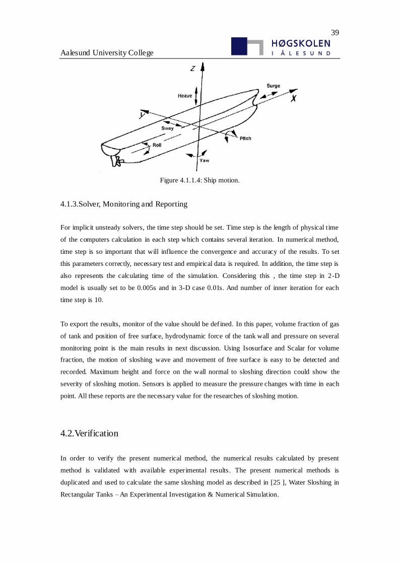
39
Aalesund University College
Figure 4.1.1.4: Ship motion.
4.1.3.Solver, Monitoring and Reporting
For implicit unsteady solvers, the time step should be set. Time step is the length of physical time
of the computers calculation in each step which contains several iteration. In numerical method,
time step is so important that will influence the convergence and accuracy of the results. To set
this parameters correctly, necessary test and empirical data is required. In addition, the time step is
also represents the calculating time of the simulation. Considering this , the time step in 2-D
model is usually set to be 0.005s and in 3-D case 0.01s. And number of inner iteration for each
time step is 10.
To export the results, monitor of the value should be defined. In this paper, volume fraction of gas
of tank and position of free surface, hydrodynamic force of the tank wall and pressure on several
monitoring point is the main results in next discussion. Using Isosurface and Scalar for volume
fraction, the motion of sloshing wave and movement of free surface is easy to be detected and
recorded. Maximum height and force on the wall normal to sloshing direction could show the
severity of sloshing motion. Sensors is applied to measure the pressure changes with time in each
point. All these reports are the necessary value for the researches of sloshing motion.
4.2.Verification
In order to verify the present numerical method, the numerical results calculated by present
method is validated with available experimental results. The present numerical methods is
duplicated and used to calculate the same sloshing model as described in [25 ], Water Sloshing in
Rectangular Tanks – An Experimental Investigation & Numerical Simulation.
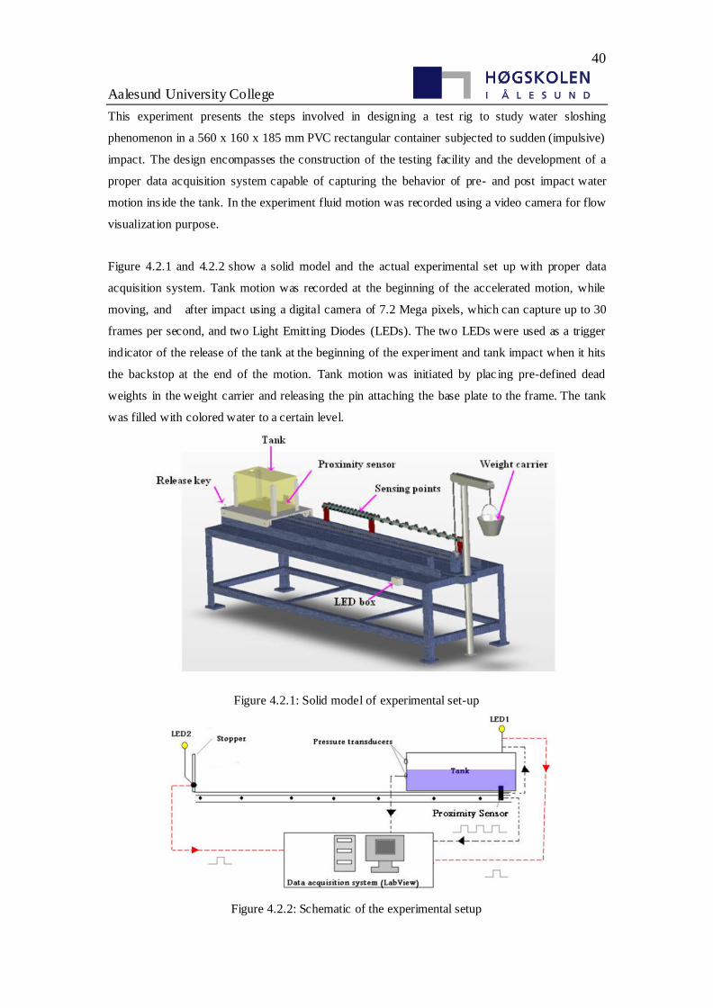
40
Aalesund University College
This experiment presents the steps involved in designing a test rig to study water sloshing
phenomenon in a 560 x 160 x 185 mm PVC rectangular container subjected to sudden (impulsive)
impact. The design encompasses the construction of the testing facility and the development of a
proper data acquisition system capable of capturing the behavior of pre- and post impact water
motion ins ide the tank. In the experiment fluid motion was recorded using a video camera for flow
visualization purpose.
Figure 4.2.1 and 4.2.2 show a solid model and the actual experimental set up with proper data
acquisition system. Tank motion was recorded at the beginning of the accelerated motion, while
moving, and after impact using a digital camera of 7.2 Mega pixels, which can capture up to 30
frames per second, and two Light Emitting Diodes (LEDs). The two LEDs were used as a trigger
indicator of the release of the tank at the beginning of the experiment and tank impact when it hits
the backstop at the end of the motion. Tank motion was initiated by plac ing pre-defined dead
weights in the weight carrier and releasing the pin attaching the base plate to the frame. The tank
was filled with colored water to a certain level.
Figure 4.2.1: Solid model of experimental set-up
Figure 4.2.2: Schematic of the experimental setup
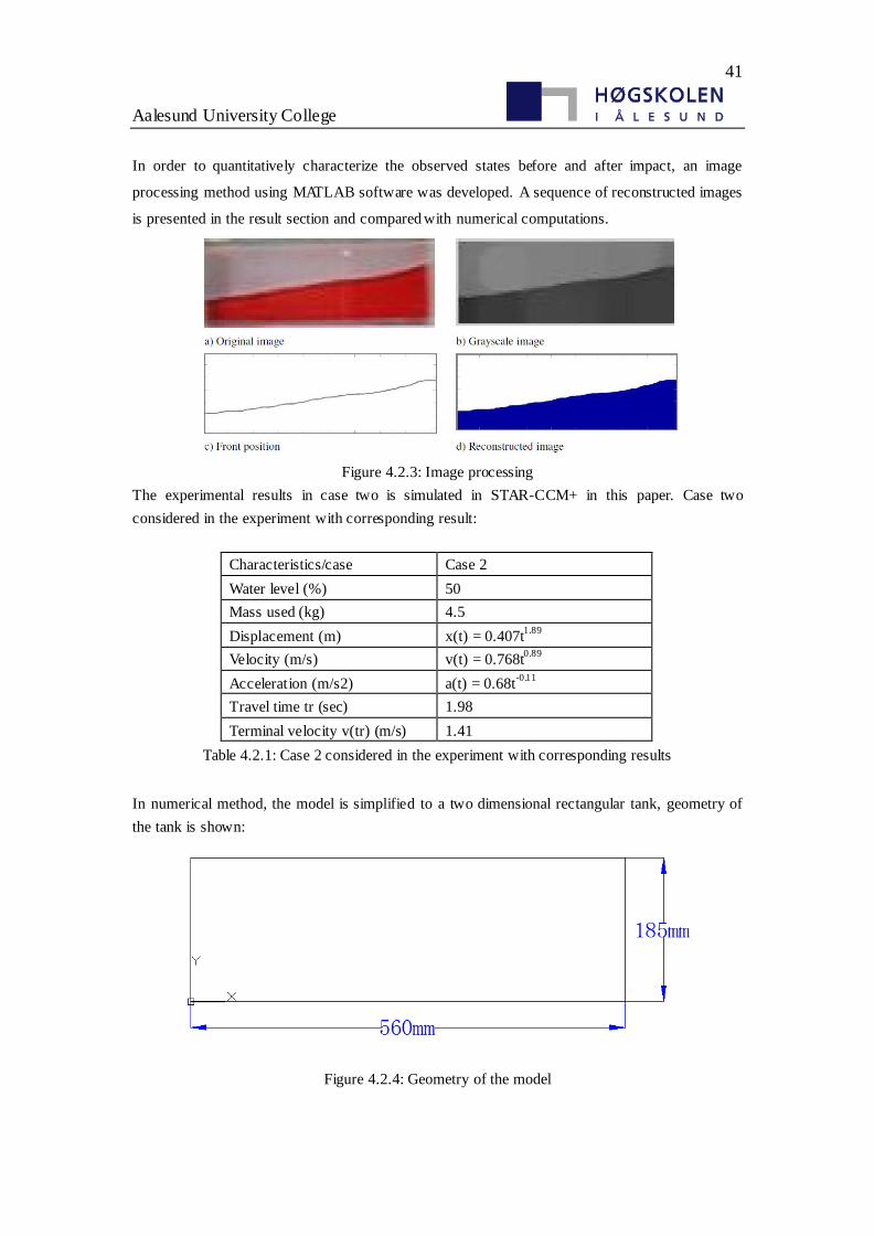
41
Aalesund University College
In order to quantitatively characterize the observed states before and after impact, an image
processing method using MATLAB software was developed. A sequence of reconstructed images
is presented in the result section and compared with numerical computations.
Figure 4.2.3: Image processing
The experimental results in case two is simulated in STAR-CCM+ in this paper. Case two
considered in the experiment with corresponding result:
Characteristics/case Case 2
Water level (%) 50
Mass used (kg) 4.5
Displacement (m) x(t) = 0.407t1.89
Velocity (m/s) v(t) = 0.768t0.89
Acceleration (m/s2) a(t) = 0.68t-0.11
Travel time tr (sec) 1.98
Terminal velocity v(tr) (m/s) 1.41
Table 4.2.1: Case 2 considered in the experiment with corresponding results
In numerical method, the model is simplified to a two dimensional rectangular tank, geometry of
the tank is shown:
Figure 4.2.4: Geometry of the model
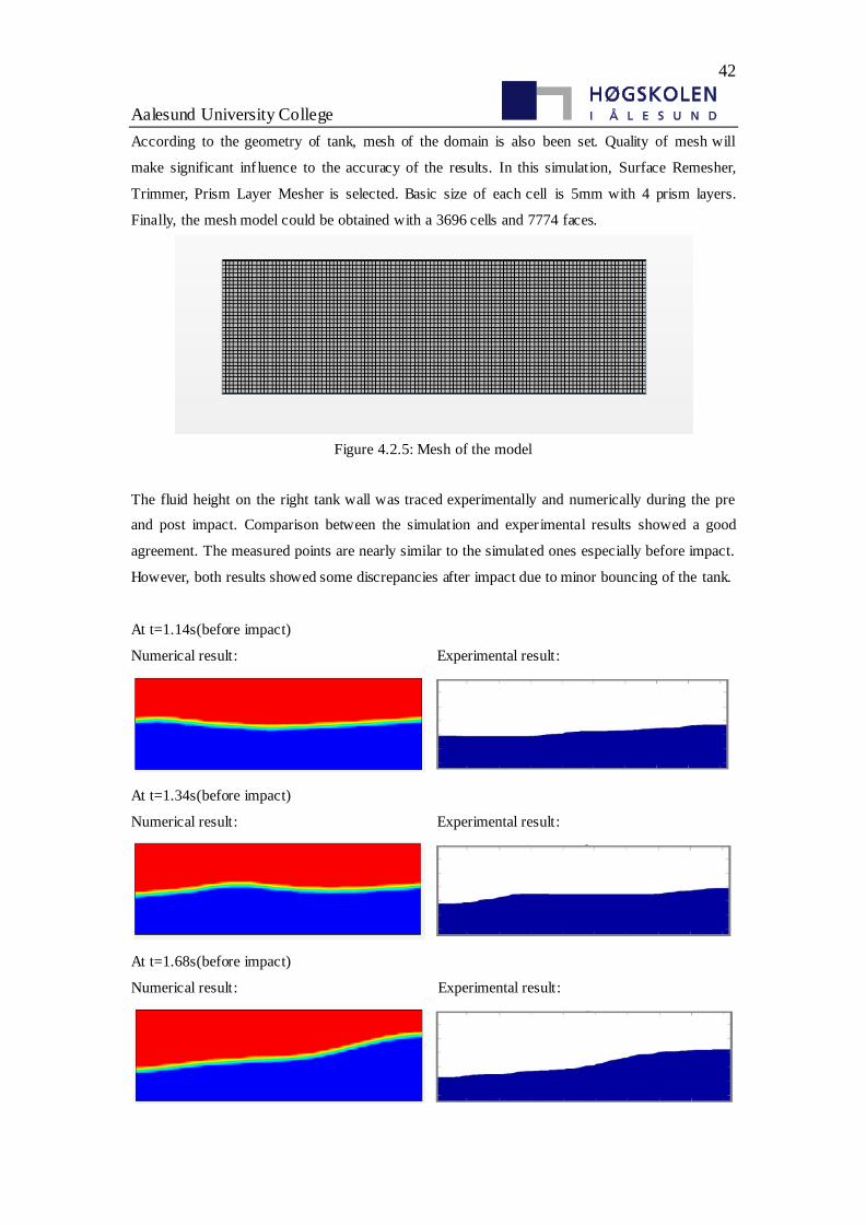
42
Aalesund University College
According to the geometry of tank, mesh of the domain is also been set. Quality of mesh will
make significant influence to the accuracy of the results. In this simulation, Surface Remesher,
Trimmer, Prism Layer Mesher is selected. Basic size of each cell is 5mm with 4 prism layers.
Finally, the mesh model could be obtained with a 3696 cells and 7774 faces.
Figure 4.2.5: Mesh of the model
The fluid height on the right tank wall was traced experimentally and numerically during the pre
and post impact. Comparison between the simulation and experimental results showed a good
agreement. The measured points are nearly similar to the simulated ones especially before impact.
However, both results showed some discrepancies after impact due to minor bouncing of the tank.
At t=1.14s(before impact)
Numerical result: Experimental result:
At t=1.34s(before impact)
Numerical result: Experimental result:
At t=1.68s(before impact)
Numerical result: Experimental result:
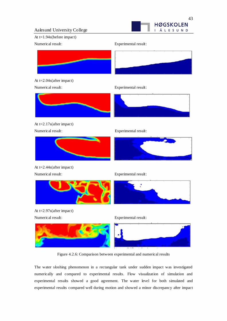
43
Aalesund University College
At t=1.94s(before impact)
Numerical result: Experimental result:
At t=2.04s(after impact)
Numerical result: Experimental result:
At t=2.17s(after impact)
Numerical result: Experimental result:
At t=2.44s(after impact)
Numerical result: Experimental result:
At t=2.97s(after impact)
Numerical result: Experimental result:
Figure 4.2.6: Comparison between experimental and numerical results
The water sloshing phenomenon in a rectangular tank under sudden impact was investigated
numerically and compared to experimental results. Flow visualization of simulation and
experimental results showed a good agreement. The water level for both simulated and
experimental results compared well during motion and showed a minor discrepancy after impact
44
Aalesund University College
which may be due to tank bouncing. In the numerical simulation and experiment, the presence of a
single traveling wave before impact is one of the situation discussed in chapter 3. In a word, the
present numerical method is validated by published experiment that simulation in next chapters
could be carried out follow this setting.
4.3.Natural Frequency
To present the critical situation for sloshing load, the most severe sloshing motion should be found
and simulated. Generally, when the frequency of excitation motion of tank is close to the natural
frequency of liquid in this tank, the resonance motion will occur that the largest motion of liquid
and sloshing load to the wall will be obtained. Thus in this part, the natural frequency of tanks will
be calculated and validated through numerical method. The liquid in this part is water, after that a
verification of LNG will also be carried out.
4.3.1.Transverse Direction
According to [26] of the empirical formula. Natural frequency of partly filled rectangular tank
should be:
1 tanh( / )
2n
ng n a bf
b
(4.1)
where
a is the level of liquid filling.
b is the length of tank in sloshing direction.
n is the order of wave.
g is gravity.
In this case, the model is a prismatic tank chose as two dimension, geometry of the model is given:
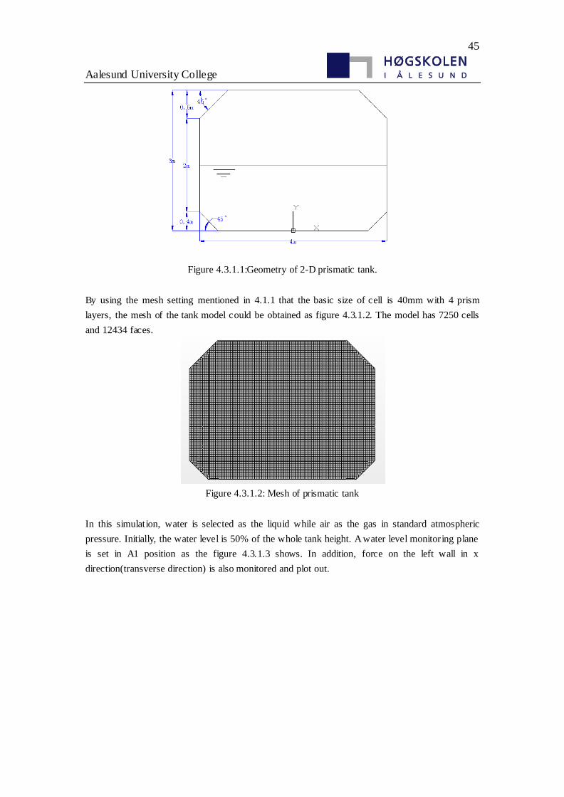
45
Aalesund University College
Figure 4.3.1.1:Geometry of 2-D prismatic tank.
By using the mesh setting mentioned in 4.1.1 that the basic size of cell is 40mm with 4 prism
layers, the mesh of the tank model could be obtained as figure 4.3.1.2. The model has 7250 cells
and 12434 faces.
Figure 4.3.1.2: Mesh of prismatic tank
In this simulation, water is selected as the liquid while air as the gas in standard atmospheric
pressure. Initially, the water level is 50% of the whole tank height. A water level monitoring plane
is set in A1 position as the figure 4.3.1.3 shows. In addition, force on the left wall in x
direction(transverse direction) is also monitored and plot out.
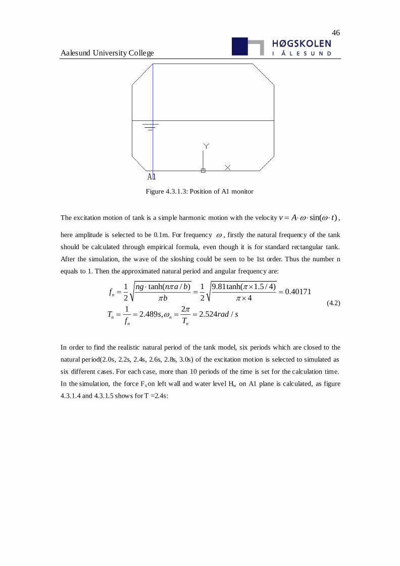
46
Aalesund University College
Figure 4.3.1.3: Position of A1 monitor
The excitation motion of tank is a simple harmonic motion with the velocity sin( )v A t ,
here amplitude is selected to be 0.1m. For frequency , firstly the natural frequency of the tank
should be calculated through empirical formula, even though it is for standard rectangular tank.
After the simulation, the wave of the sloshing could be seen to be 1st order. Thus the number n
equals to 1. Then the approximated natural period and angular frequency are:
1 tanh( / ) 1 9.81tanh( 1.5 / 4)0.40171
2 2 4
1 22.489 , 2.524 /
n
n n
n n
ng n a bf
b
T s rad sf T
(4.2)
In order to find the realistic natural period of the tank model, six periods which are closed to the
natural period(2.0s, 2.2s, 2.4s, 2.6s, 2.8s, 3.0s) of the excitation motion is selected to simulated as
six different cases. For each case, more than 10 periods of the time is set for the calculation time.
In the simulation, the force Fx on left wall and water level Hw on A1 plane is calculated, as figure
4.3.1.4 and 4.3.1.5 shows for T =2.4s:
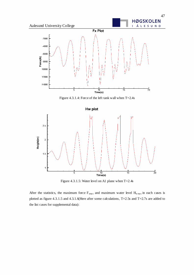
47
Aalesund University College
Figure 4.3.1.4: Force of the left tank wall when T=2.4s
Figure 4.3.1.5: Water level on A1 plane when T=2.4s
After the statistics, the maximum force Fxmax and maximum water level Hw max in each cases is
plotted as figure 4.3.1.5 and 4.3.1.6(Here after some calculations, T=2.5s and T=2.7s are added to
the list cases for supplemental data):
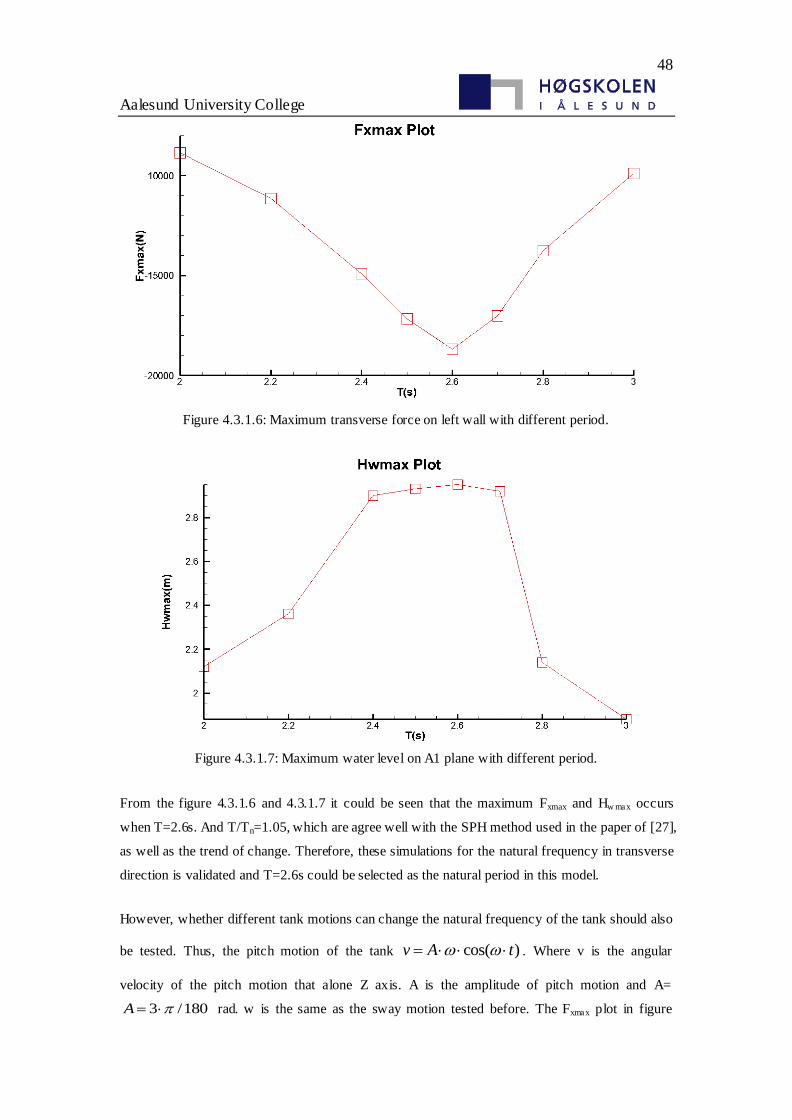
48
Aalesund University College
Figure 4.3.1.6: Maximum transverse force on left wall with different period.
Figure 4.3.1.7: Maximum water level on A1 plane with different period.
From the figure 4.3.1.6 and 4.3.1.7 it could be seen that the maximum Fxmax and Hw max occurs
when T=2.6s. And T/Tn=1.05, which are agree well with the SPH method used in the paper of [27],
as well as the trend of change. Therefore, these simulations for the natural frequency in transverse
direction is validated and T=2.6s could be selected as the natural period in this model.
However, whether different tank motions can change the natural frequency of the tank should also
be tested. Thus, the pitch motion of the tank cos( )v A t . Where v is the angular
velocity of the pitch motion that alone Z axis. A is the amplitude of pitch motion and A=
3 /180A rad. w is the same as the sway motion tested before. The Fxmax plot in figure
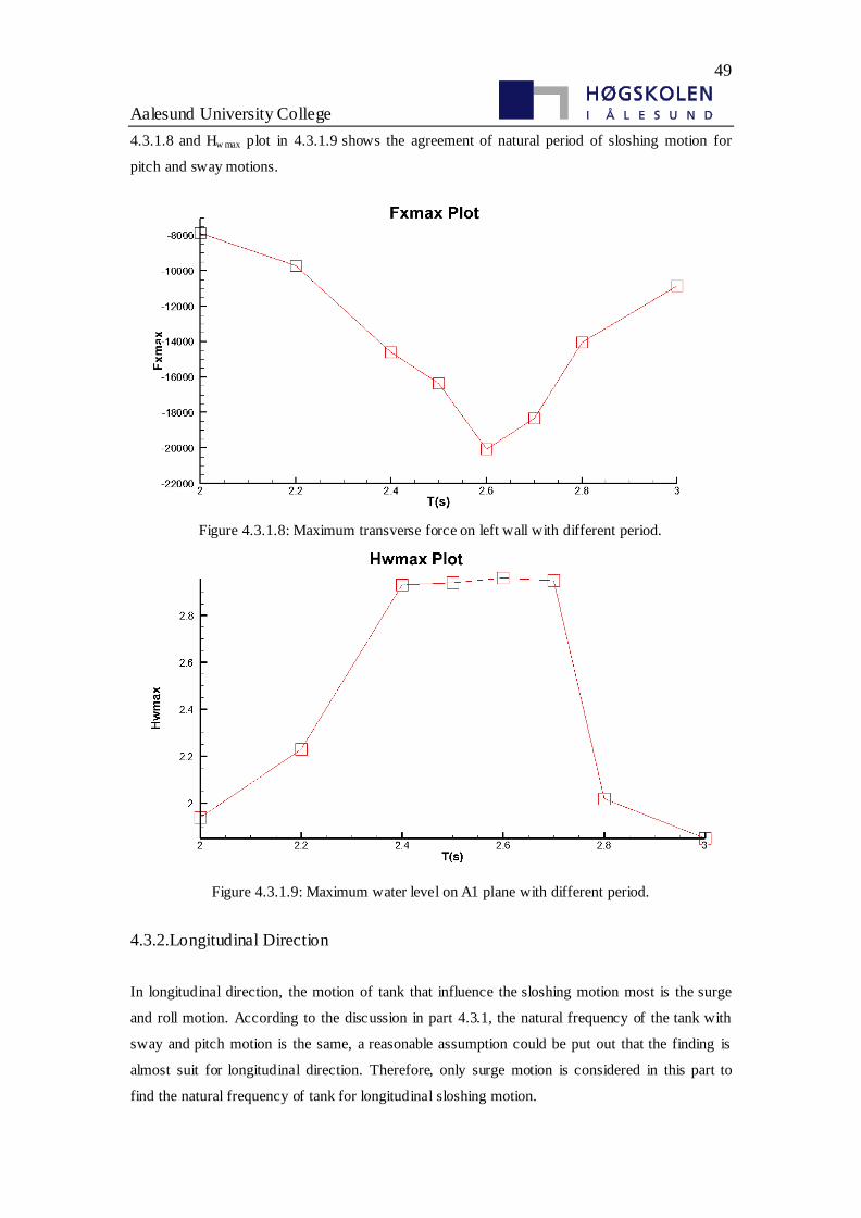
49
Aalesund University College
4.3.1.8 and Hw max plot in 4.3.1.9 shows the agreement of natural period of sloshing motion for
pitch and sway motions.
Figure 4.3.1.8: Maximum transverse force on left wall with different period.
Figure 4.3.1.9: Maximum water level on A1 plane with different period.
4.3.2.Longitudinal Direction
In longitudinal direction, the motion of tank that influence the sloshing motion most is the surge
and roll motion. According to the discussion in part 4.3.1, the natural frequency of the tank with
sway and pitch motion is the same, a reasonable assumption could be put out that the finding is
almost suit for longitudinal direction. Therefore, only surge motion is considered in this part to
find the natural frequency of tank for longitudinal sloshing motion.
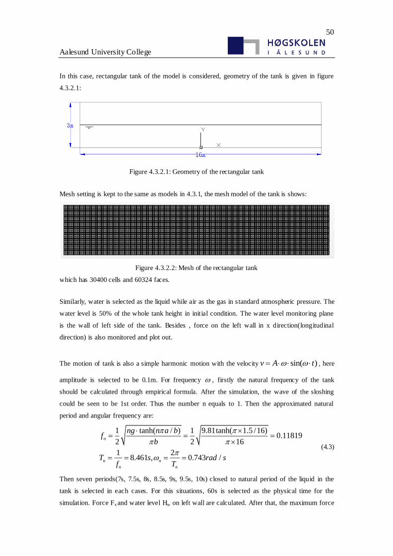
50
Aalesund University College
In this case, rectangular tank of the model is considered, geometry of the tank is given in figure
4.3.2.1:
Figure 4.3.2.1: Geometry of the rectangular tank
Mesh setting is kept to the same as models in 4.3.1, the mesh model of the tank is shows:
Figure 4.3.2.2: Mesh of the rectangular tank
which has 30400 cells and 60324 faces.
Similarly, water is selected as the liquid while air as the gas in standard atmospheric pressure. The
water level is 50% of the whole tank height in initial condition. The water level monitoring plane
is the wall of left side of the tank. Besides , force on the left wall in x direction(longitudinal
direction) is also monitored and plot out.
The motion of tank is also a simple harmonic motion with the velocity sin( )v A t , here
amplitude is selected to be 0.1m. For frequency , firstly the natural frequency of the tank
should be calculated through empirical formula. After the simulation, the wave of the sloshing
could be seen to be 1st order. Thus the number n equals to 1. Then the approximated natural
period and angular frequency are:
1 tanh( / ) 1 9.81tanh( 1.5 /16)0.11819
2 2 16
1 28.461 , 0.743 /
n
n n
n n
ng n a bf
b
T s rad sf T
(4.3)
Then seven periods(7s, 7.5s, 8s, 8.5s, 9s, 9.5s, 10s) closed to natural period of the liquid in the
tank is selected in each cases. For this situations, 60s is selected as the physical time for the
simulation. Force Fx and water level Hw on left wall are calculated. After that, the maximum force
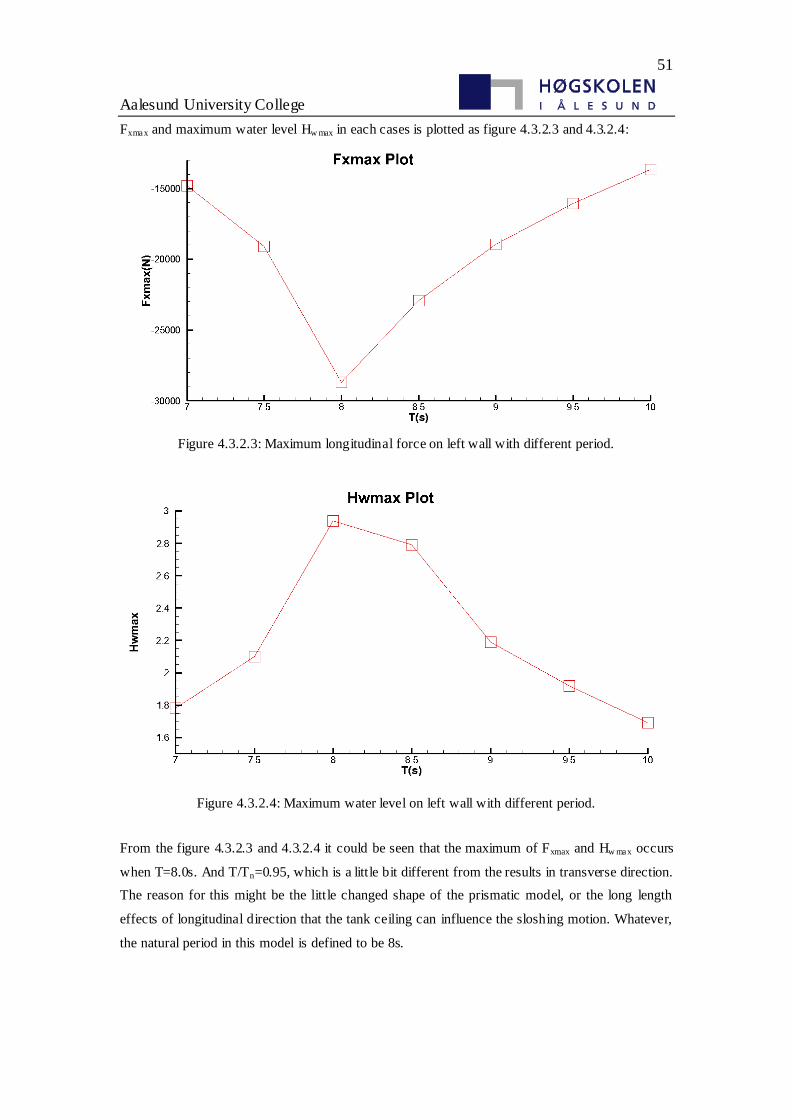
51
Aalesund University College
Fxmax and maximum water level Hw max in each cases is plotted as figure 4.3.2.3 and 4.3.2.4:
Figure 4.3.2.3: Maximum longitudinal force on left wall with different period.
Figure 4.3.2.4: Maximum water level on left wall with different period.
From the figure 4.3.2.3 and 4.3.2.4 it could be seen that the maximum of Fxmax and Hw max occurs
when T=8.0s. And T/Tn=0.95, which is a little bit different from the results in transverse direction.
The reason for this might be the little changed shape of the prismatic model, or the long length
effects of longitudinal direction that the tank ceiling can influence the sloshing motion. Whatever,
the natural period in this model is defined to be 8s.
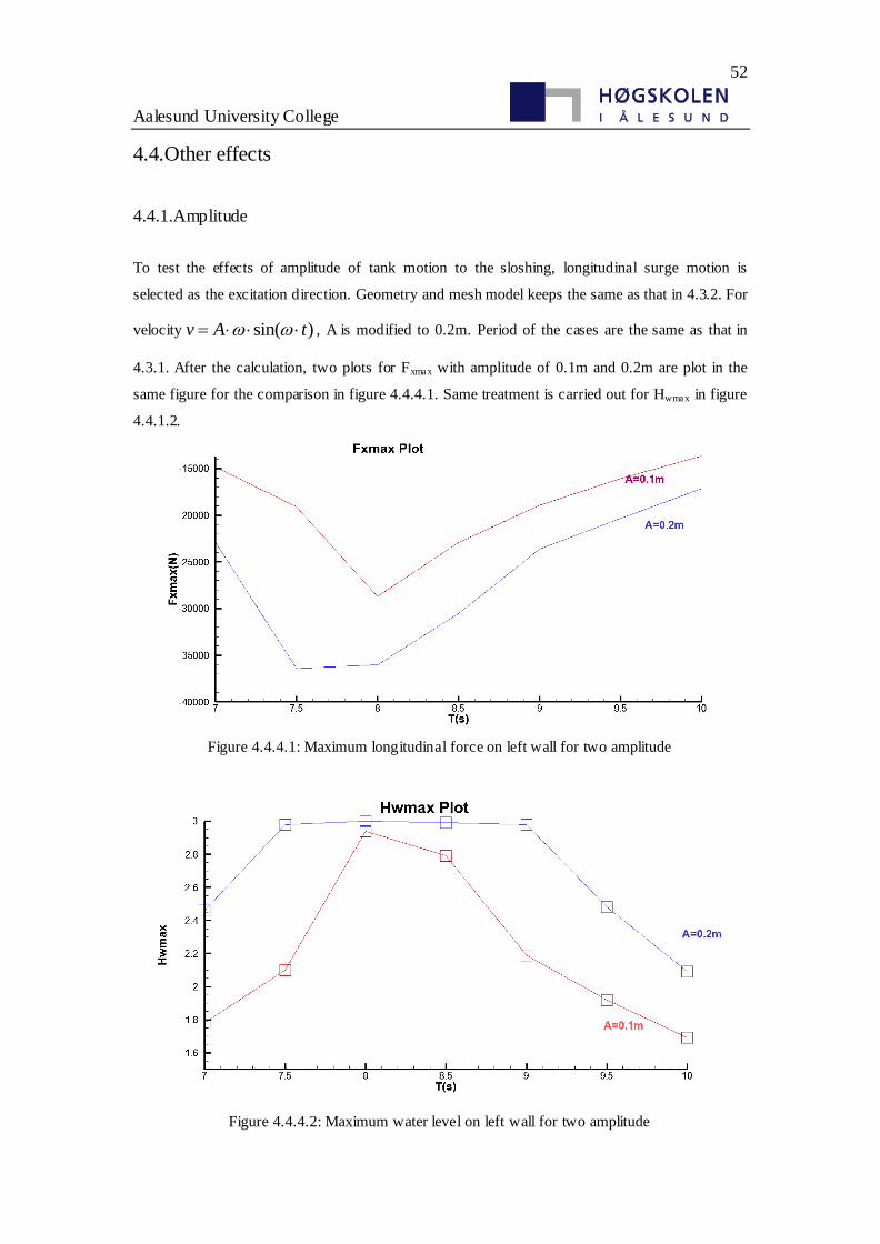
52
Aalesund University College
4.4.Other effects
4.4.1.Amplitude
To test the effects of amplitude of tank motion to the sloshing, longitudinal surge motion is
selected as the excitation direction. Geometry and mesh model keeps the same as that in 4.3.2. For
velocity sin( )v A t , A is modified to 0.2m. Period of the cases are the same as that in
4.3.1. After the calculation, two plots for Fxmax with amplitude of 0.1m and 0.2m are plot in the
same figure for the comparison in figure 4.4.4.1. Same treatment is carried out for Hwmax in figure
4.4.1.2.
Figure 4.4.4.1: Maximum longitudinal force on left wall for two amplitude
Figure 4.4.4.2: Maximum water level on left wall for two amplitude
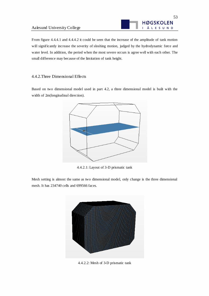
53
Aalesund University College
From figure 4.4.4.1 and 4.4.4.2 it could be seen that the increase of the amplitude of tank motion
will signif icantly increase the severity of sloshing motion, judged by the hydrodynamic force and
water level. In addition, the period when the most severe occurs is agree well with each other. The
small difference may because of the limitation of tank height.
4.4.2.Three Dimensional Effects
Based on two dimensional model used in part 4.2, a three dimensional model is built with the
width of 2m(longitudinal direction).
4.4.2.1: Layout of 3-D prismatic tank
Mesh setting is almost the same as two dimensional model, only change is the three dimensional
mesh. It has 234740 cells and 699566 faces.
4.4.2.2: Mesh of 3-D prismatic tank
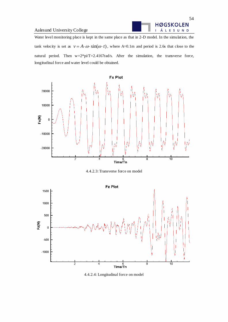
54
Aalesund University College
Water level monitoring place is kept in the same place as that in 2-D model. In the simulation, the
tank velocity is set as sin( )v A t , where A=0.1m and period is 2.6s that close to the
natural period. Then w=2*pi/T=2.4167rad/s. After the simulation, the transverse force,
longitudinal force and water level could be obtained.
4.4.2.3: Transverse force on model
4.4.2.4: Longitudinal force on model
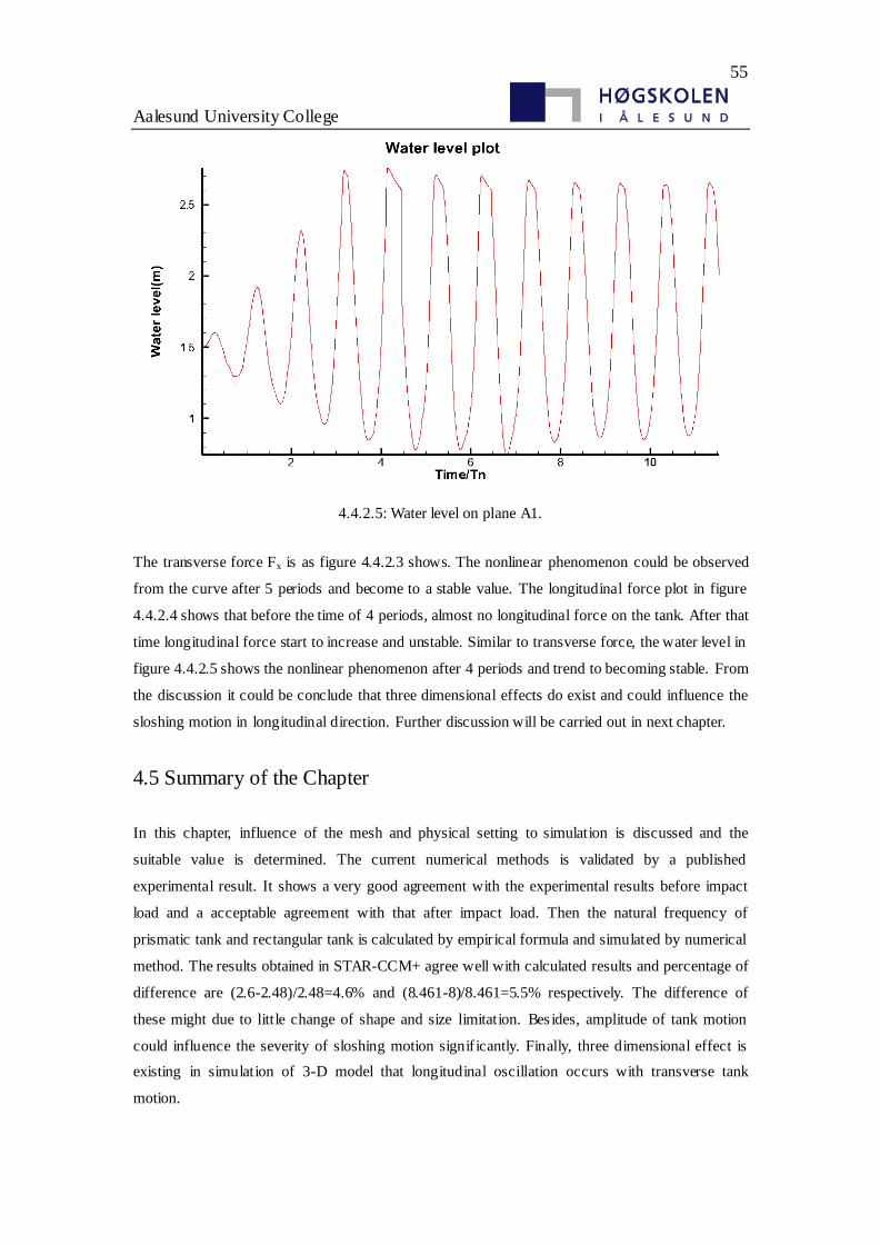
55
Aalesund University College
4.4.2.5: Water level on plane A1.
The transverse force Fx is as figure 4.4.2.3 shows. The nonlinear phenomenon could be observed
from the curve after 5 periods and become to a stable value. The longitudinal force plot in figure
4.4.2.4 shows that before the time of 4 periods, almost no longitudinal force on the tank. After that
time longitudinal force start to increase and unstable. Similar to transverse force, the water level in
figure 4.4.2.5 shows the nonlinear phenomenon after 4 periods and trend to becoming stable. From
the discussion it could be conclude that three dimensional effects do exist and could influence the
sloshing motion in longitudinal direction. Further discussion will be carried out in next chapter.
4.5 Summary of the Chapter
In this chapter, influence of the mesh and physical setting to simulation is discussed and the
suitable value is determined. The current numerical methods is validated by a published
experimental result. It shows a very good agreement with the experimental results before impact
load and a acceptable agreement with that after impact load. Then the natural frequency of
prismatic tank and rectangular tank is calculated by empirical formula and simulated by numerical
method. The results obtained in STAR-CCM+ agree well with calculated results and percentage of
difference are (2.6-2.48)/2.48=4.6% and (8.461-8)/8.461=5.5% respectively. The difference of
these might due to little change of shape and size limitation. Bes ides, amplitude of tank motion
could influence the severity of sloshing motion signif icantly. Finally, three dimensional effect is
existing in simulation of 3-D model that longitudinal oscillation occurs with transverse tank
motion.
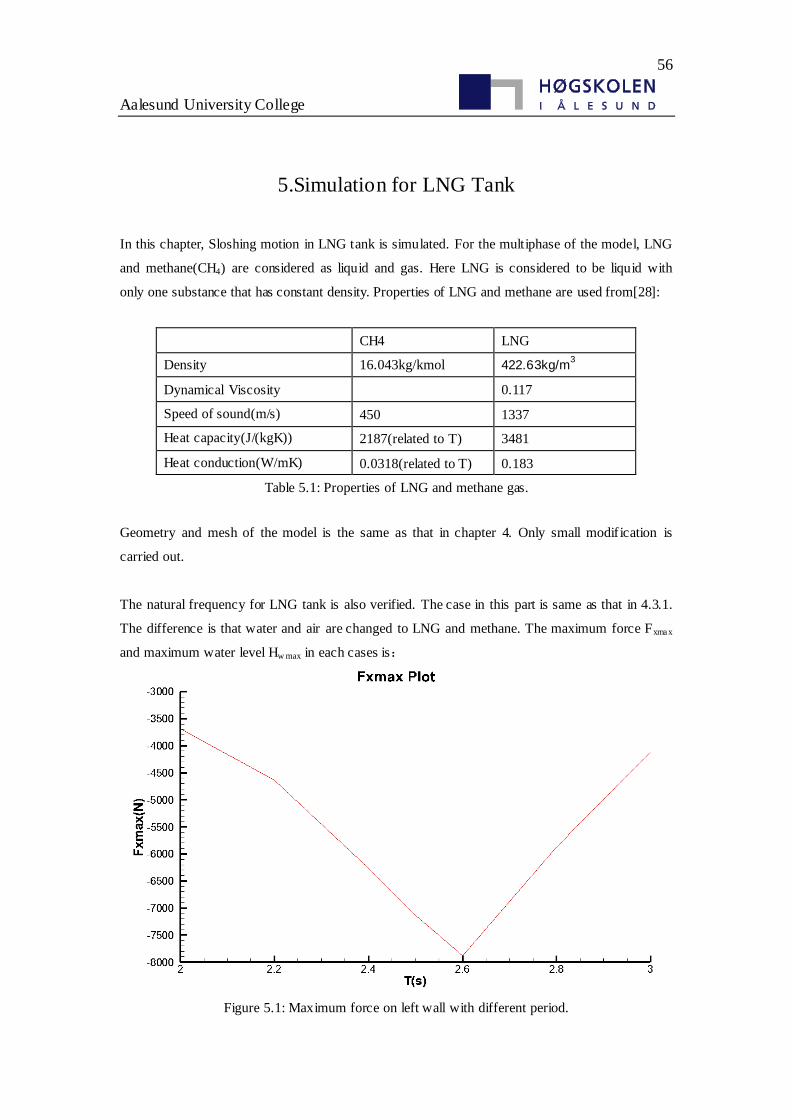
56
Aalesund University College
5.Simulation for LNG Tank
In this chapter, Sloshing motion in LNG tank is simulated. For the multiphase of the model, LNG
and methane(CH4) are considered as liquid and gas. Here LNG is considered to be liquid with
only one substance that has constant density. Properties of LNG and methane are used from[28]:
CH4 LNG
Density 16.043kg/kmol 422.63kg/m3
Dynamical Viscosity 0.117
Speed of sound(m/s) 450 1337
Heat capacity(J/(kgK)) 2187(related to T) 3481
Heat conduction(W/mK) 0.0318(related to T) 0.183
Table 5.1: Properties of LNG and methane gas.
Geometry and mesh of the model is the same as that in chapter 4. Only small modification is
carried out.
The natural frequency for LNG tank is also verified. The case in this part is same as that in 4.3.1.
The difference is that water and air are changed to LNG and methane. The maximum force Fxmax
and maximum water level Hw max in each cases is:
Figure 5.1: Maximum force on left wall with different period.
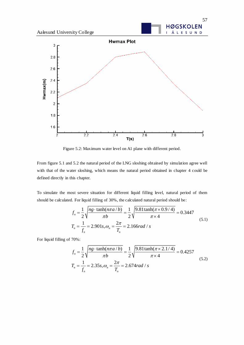
57
Aalesund University College
Figure 5.2: Maximum water level on A1 plane with different period.
From figure 5.1 and 5.2 the natural period of the LNG sloshing obtained by simulation agree well
with that of the water sloshing, which means the natural period obtained in chapter 4 could be
defined directly in this chapter.
To simulate the most severe situation for different liquid filling level, natural period of them
should be calculated. For liquid filling of 30%, the calculated natural period should be:
1 tanh( / ) 1 9.81tanh( 0.9 / 4)0.3447
2 2 4
1 22.901 , 2.166 /
n
n n
n n
ng n a bf
b
T s rad sf T
(5.1)
For liquid filling of 70%:
1 tanh( / ) 1 9.81tanh( 2.1/ 4)0.4257
2 2 4
1 22.35 , 2.674 /
n
n n
n n
ng n a bf
b
T s rad sf T
(5.2)
58
Aalesund University College
5.1 Prismatic and Rectangular Tanks
5.1.1. Two dimension
In order to find the pressure distribution and movement of free surface with different kinds of tank
motions, different amplitudes and different liquid filling levels, a series of simulations are carried
out and compared with related cases. Positions of sensors to monitor the pressure is shown in
figure 5.1.1.1. Simulated cases considered in this part are tabulated in table 5.1.1.1:
Figure 5.1.1.1: Position of the sensors.
Case Filling level(h/H) Motion Amplitude Excitation Period(s)
1 30 0.1m 2.9
2 30 0.05m 2.9
3 30 0.1m 2.6
4 50 0.1m 2.6
5 70 0.1m 2.34
6 30 3deg 2.9
7 30 2deg 2.9
8 50 3deg 2.6
9 50 2deg 2.6
10 70 3deg 2.34
Table 5.1.1.1: Summary of some of the cases.
After the simulation, the impact pressure on sensor 2-4 with three liquid fillings is plot. Figure
5.1.1.2 is the plot for sway tank motion(case1,4,5). Figure 5.1.1.3 is the plot for pitch motion(case
6,8,10). These figures illustrate the impact pressure during the sloshing motion. Comparing the
59
Aalesund University College
two figures, it could be found that a lower liquid filling level could induce a larger impact pressure.
Because the position of sensors are in the same height as the liquid level in each case respectively,
the pressure measured by the sensors is the impact force only.
Figure 5.1.1.2: Pressure on different sensor for different cases respectively with sway motion.
Figure 5.1.1.3: Pressure on different sensor for different cases respectively with pitch motion.
Figure 5.1.1.4 shows the movement and deformation of the free surface in each time for case
1,case 4 and case 5. It could be seen from the figure that the increase of the liquid depth will
increase the nonlinearity of the liquid motion. At 50% and 70% liquid fillings, the wave breaking
and liquid splashing phenomenon could be easily observed.
60
Aalesund University College
Figure 5.1.1.4: Movement of free surface for case1(left) case4(middle) and case5(right) .
5.1.2 Baffle Effects
The inner structure of the tank--baffle is used to reduce the sloshing motion and produced impact
force. Influence of the baffle to the tank in sloshing is simulated and tested. Position and size of
the baffle is given in figure 5.1.2.1. Added cases contain baffle are also carried out in table 5.1.2.1.
61
Aalesund University College
Figure 5.1.2.1: Position and size of baffle.
Case Filling level(h/H) Motion Amplitude Excitation Period(s)
11 50 0.1m 2.6
12 50 0.1m 2.0
13 50 0.1m 2.2
14 50 0.1m 1.6
15 50 0.1m 1.2
16 50 0.1m 1.0
17 50 0.1m 1.4
18 50 0.1m 1.3
19 50 0.1m 1.1
Table 5.1.2.2: Summary of some of the cases for natural period with baffle.
Assuming that the baffle is high enough that this tank will be divided into two separated tanks,
natural frequency for each separated tank is obviously different from the initial tank. Thus, in our
case, the natural frequency should also be changed to some degree. Then the cases 11-19 are used
to find the new natural frequency for the modified tank.
After simulations, the pressure changed during simulation on each sensor could be plot by the
software. Here sensor 3 is chosen to be the monitor. The maximum pressure on sensor 3 is
obtained through the plot and a new plot shows the maximum pressure during the simulation for
different period is given in figure 5.1.2.3. From this it could be found that T=1.2s is closed to
natural period of the tank with baffle mostly.
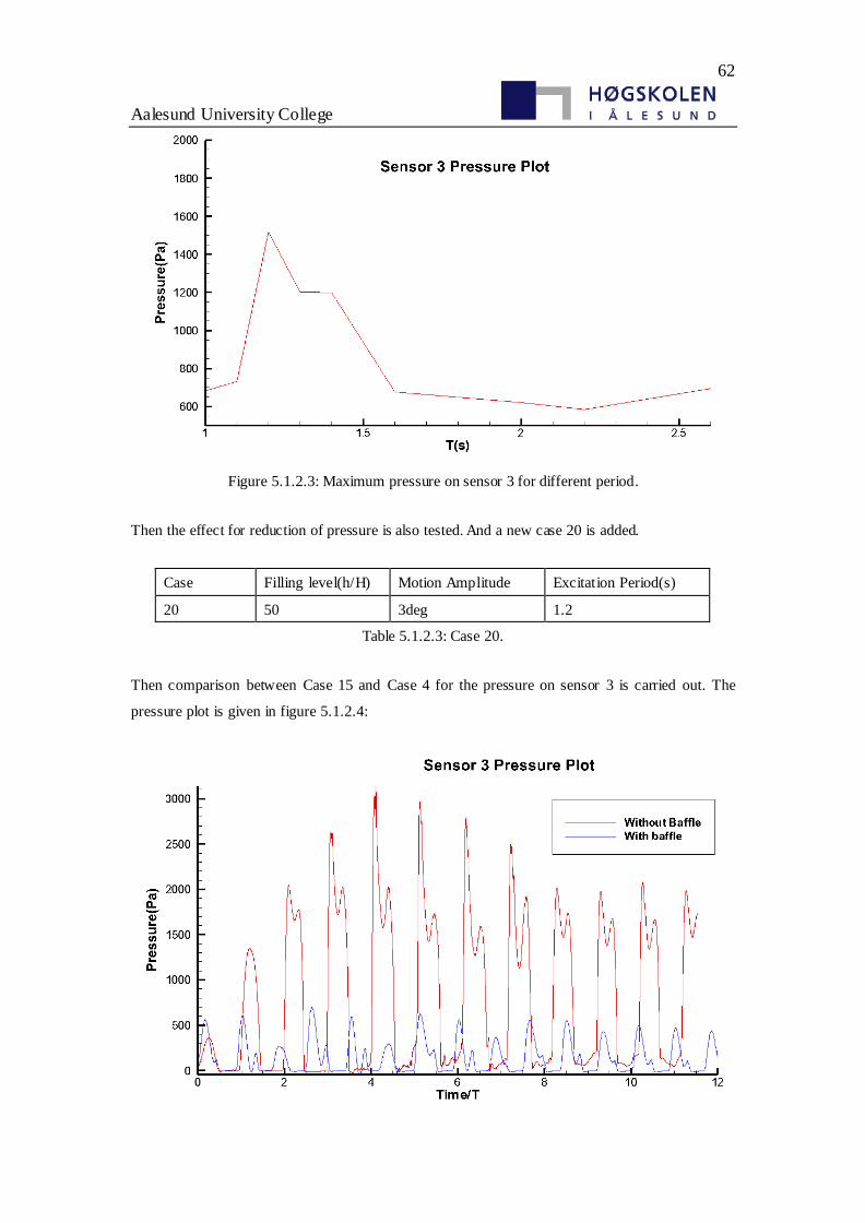
62
Aalesund University College
Figure 5.1.2.3: Maximum pressure on sensor 3 for different period.
Then the effect for reduction of pressure is also tested. And a new case 20 is added.
Case Filling level(h/H) Motion Amplitude Excitation Period(s)
20 50 3deg 1.2
Table 5.1.2.3: Case 20.
Then comparison between Case 15 and Case 4 for the pressure on sensor 3 is carried out. The
pressure plot is given in figure 5.1.2.4:
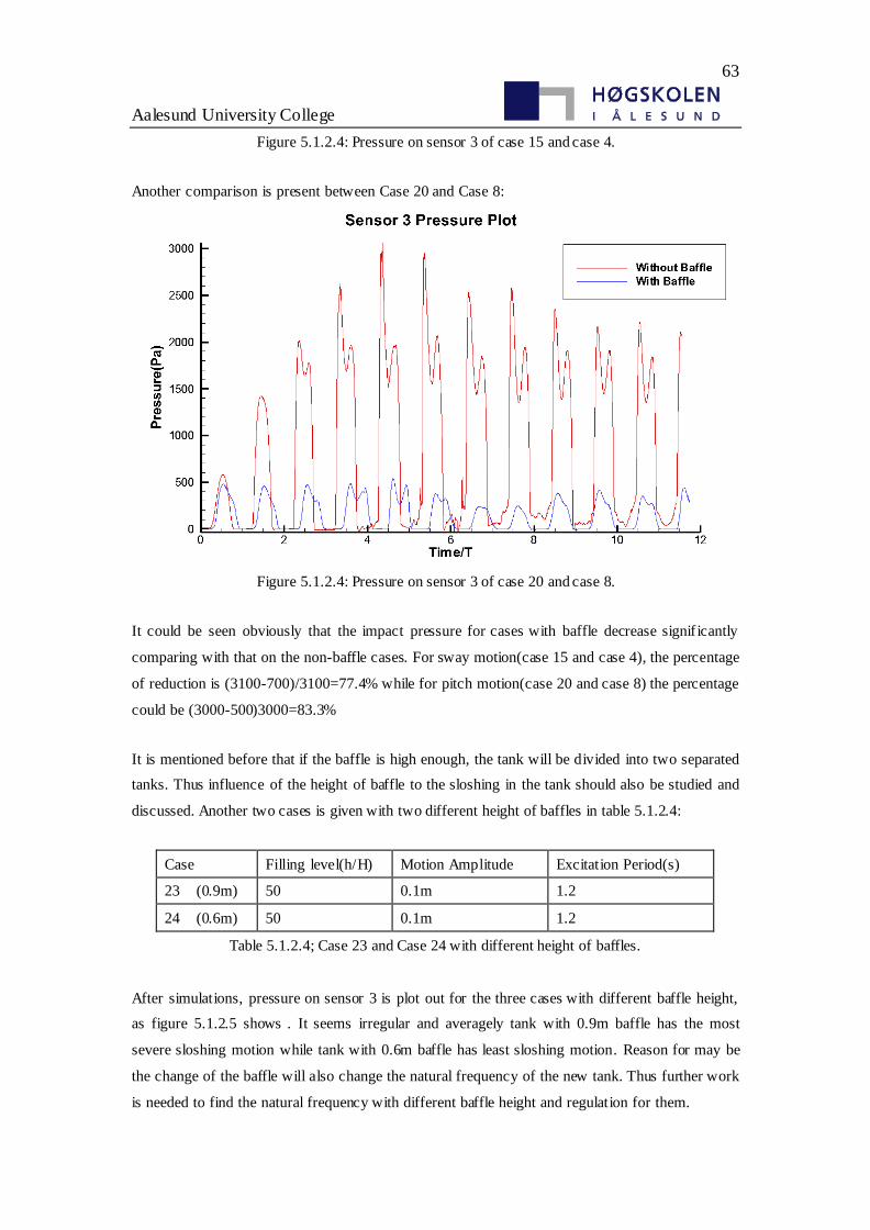
63
Aalesund University College
Figure 5.1.2.4: Pressure on sensor 3 of case 15 and case 4.
Another comparison is present between Case 20 and Case 8:
Figure 5.1.2.4: Pressure on sensor 3 of case 20 and case 8.
It could be seen obviously that the impact pressure for cases with baffle decrease signif icantly
comparing with that on the non-baffle cases. For sway motion(case 15 and case 4), the percentage
of reduction is (3100-700)/3100=77.4% while for pitch motion(case 20 and case 8) the percentage
could be (3000-500)3000=83.3%
It is mentioned before that if the baffle is high enough, the tank will be divided into two separated
tanks. Thus influence of the height of baffle to the sloshing in the tank should also be studied and
discussed. Another two cases is given with two different height of baffles in table 5.1.2.4:
Case Filling level(h/H) Motion Amplitude Excitation Period(s)
23 (0.9m) 50 0.1m 1.2
24 (0.6m) 50 0.1m 1.2
Table 5.1.2.4; Case 23 and Case 24 with different height of baffles.
After simulations, pressure on sensor 3 is plot out for the three cases with different baffle height,
as figure 5.1.2.5 shows . It seems irregular and averagely tank with 0.9m baffle has the most
severe sloshing motion while tank with 0.6m baffle has least sloshing motion. Reason for may be
the change of the baffle will also change the natural frequency of the new tank. Thus further work
is needed to find the natural frequency with different baffle height and regulation for them.
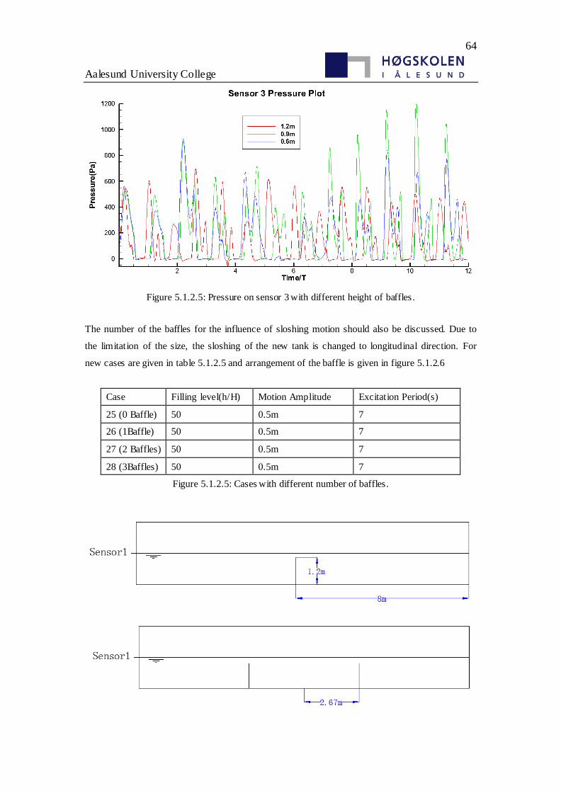
64
Aalesund University College
Figure 5.1.2.5: Pressure on sensor 3 with different height of baffles.
The number of the baffles for the influence of sloshing motion should also be discussed. Due to
the limitation of the size, the sloshing of the new tank is changed to longitudinal direction. For
new cases are given in table 5.1.2.5 and arrangement of the baffle is given in figure 5.1.2.6
Case Filling level(h/H) Motion Amplitude Excitation Period(s)
25 (0 Baffle) 50 0.5m 7
26 (1Baffle) 50 0.5m 7
27 (2 Baffles) 50 0.5m 7
28 (3Baffles) 50 0.5m 7
Figure 5.1.2.5: Cases with different number of baffles.
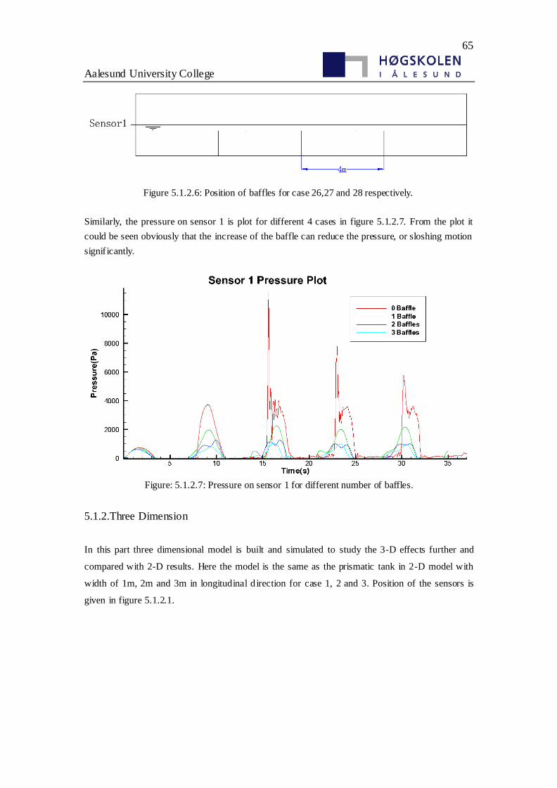
65
Aalesund University College
Figure 5.1.2.6: Position of baffles for case 26,27 and 28 respectively.
Similarly, the pressure on sensor 1 is plot for different 4 cases in figure 5.1.2.7. From the plot it
could be seen obviously that the increase of the baffle can reduce the pressure, or sloshing motion
signif icantly.
Figure: 5.1.2.7: Pressure on sensor 1 for different number of baffles.
5.1.2.Three Dimension
In this part three dimensional model is built and simulated to study the 3-D effects further and
compared with 2-D results. Here the model is the same as the prismatic tank in 2-D model with
width of 1m, 2m and 3m in longitudinal d irection for case 1, 2 and 3. Position of the sensors is
given in figure 5.1.2.1.
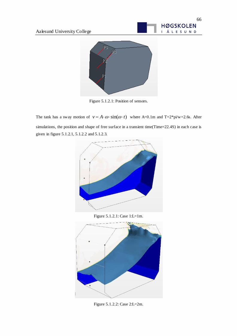
66
Aalesund University College
Figure 5.1.2.1: Position of sensors.
The tank has a sway motion of sin( )v A t where A=0.1m and T=2*pi/w=2.6s. After
simulations, the position and shape of free surface in a transient time(Time=22.4S) in each case is
given in figure 5.1.2.1, 5.1.2.2 and 5.1.2.3.
Figure 5.1.2.1: Case 1:L=1m.
Figure 5.1.2.2: Case 2:L=2m.
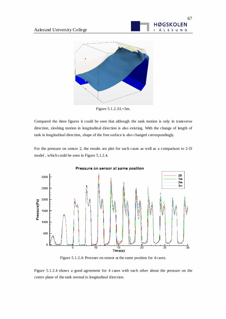
67
Aalesund University College
Figure 5.1.2.3:L=3m.
Compared the three figures it could be seen that although the tank motion is only in transverse
direction, sloshing motion in longitudinal direction is also existing. With the change of length of
tank in longitudinal direction, shape of the free surface is also changed correspondingly.
For the pressure on sensor 2, the results are plot for each cases as well as a comparison to 2-D
model , which could be seen in Figure 5.1.2.4.
Figure 5.1.2.4: Pressure on sensor at the same position for 4 cases.
Figure 5.1.2.4 shows a good agreement for 4 cases with each other about the pressure on the
centre plane of the tank normal to longitudinal direction.
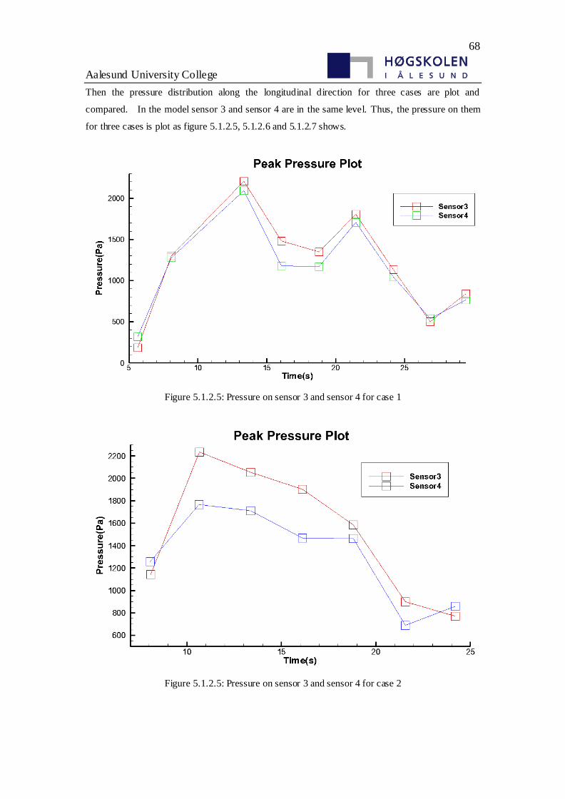
68
Aalesund University College
Then the pressure distribution along the longitudinal direction for three cases are plot and
compared. In the model sensor 3 and sensor 4 are in the same level. Thus, the pressure on them
for three cases is plot as figure 5.1.2.5, 5.1.2.6 and 5.1.2.7 shows.
Figure 5.1.2.5: Pressure on sensor 3 and sensor 4 for case 1
Figure 5.1.2.5: Pressure on sensor 3 and sensor 4 for case 2
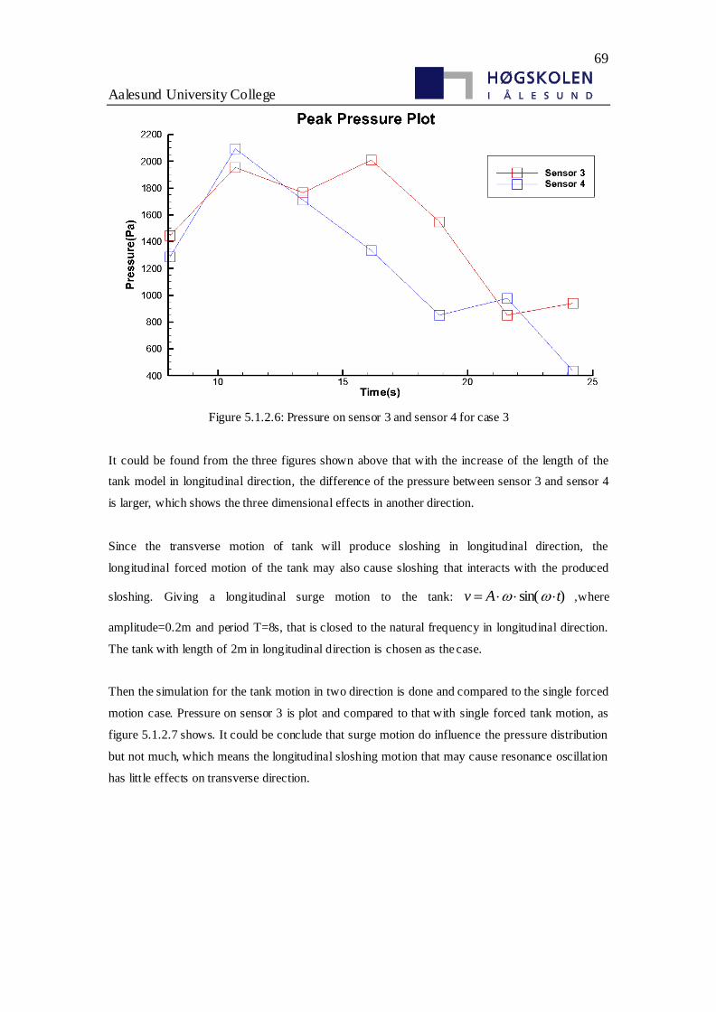
69
Aalesund University College
Figure 5.1.2.6: Pressure on sensor 3 and sensor 4 for case 3
It could be found from the three figures shown above that with the increase of the length of the
tank model in longitudinal direction, the difference of the pressure between sensor 3 and sensor 4
is larger, which shows the three dimensional effects in another direction.
Since the transverse motion of tank will produce sloshing in longitudinal direction, the
longitudinal forced motion of the tank may also cause sloshing that interacts with the produced
sloshing. Giving a longitudinal surge motion to the tank: sin( )v A t ,where
amplitude=0.2m and period T=8s, that is closed to the natural frequency in longitudinal direction.
The tank with length of 2m in longitudinal direction is chosen as the case.
Then the simulation for the tank motion in two direction is done and compared to the single forced
motion case. Pressure on sensor 3 is plot and compared to that with single forced tank motion, as
figure 5.1.2.7 shows. It could be conclude that surge motion do influence the pressure distribution
but not much, which means the longitudinal sloshing motion that may cause resonance oscillation
has little effects on transverse direction.
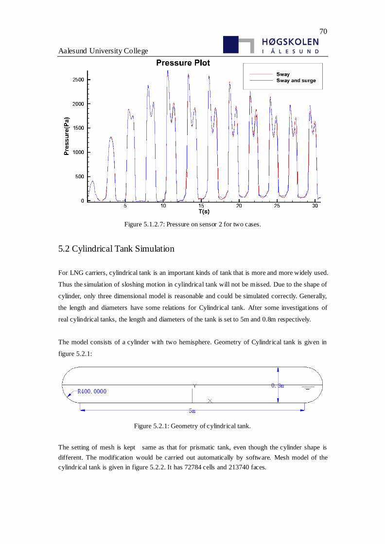
70
Aalesund University College
Figure 5.1.2.7: Pressure on sensor 2 for two cases.
5.2 Cylindrical Tank Simulation
For LNG carriers, cylindrical tank is an important kinds of tank that is more and more widely used.
Thus the simulation of sloshing motion in cylindrical tank will not be missed. Due to the shape of
cylinder, only three dimensional model is reasonable and could be simulated correctly. Generally,
the length and diameters have some relations for Cylindrical tank. After some investigations of
real cylindrical tanks, the length and diameters of the tank is set to 5m and 0.8m respectively.
The model consists of a cylinder with two hemisphere. Geometry of Cylindrical tank is given in
figure 5.2.1:
Figure 5.2.1: Geometry of cylindrical tank.
The setting of mesh is kept same as that for prismatic tank, even though the cylinder shape is
different. The modification would be carried out automatically by software. Mesh model of the
cylindrical tank is given in figure 5.2.2. It has 72784 cells and 213740 faces.
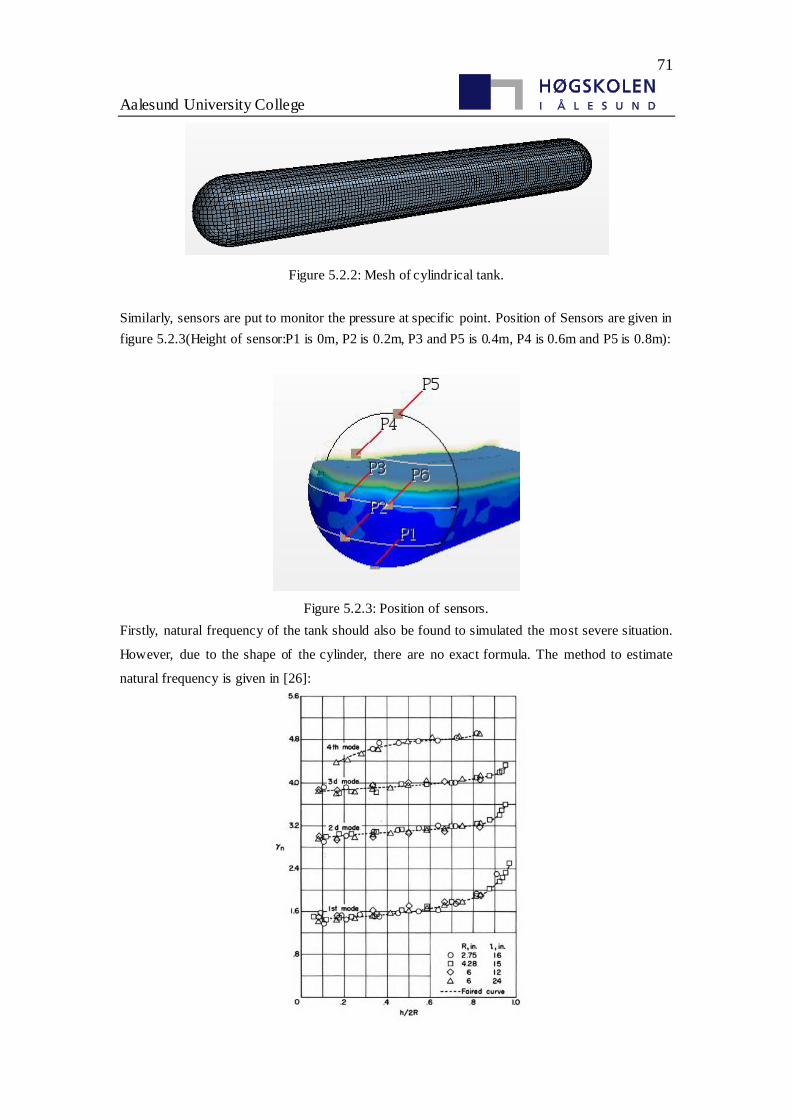
71
Aalesund University College
Figure 5.2.2: Mesh of cylindrical tank.
Similarly, sensors are put to monitor the pressure at specific point. Position of Sensors are given in
figure 5.2.3(Height of sensor:P1 is 0m, P2 is 0.2m, P3 and P5 is 0.4m, P4 is 0.6m and P5 is 0.8m):
Figure 5.2.3: Position of sensors.
Firstly, natural frequency of the tank should also be found to simulated the most severe situation.
However, due to the shape of the cylinder, there are no exact formula. The method to estimate
natural frequency is given in [26]:
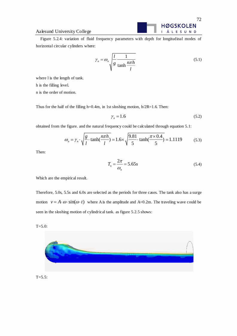
72
Aalesund University College
Figure 5.2.4: variation of fluid frequency parameters with depth for longitudinal modes of
horizontal circular cylinders where:
1
tanhn n
l
n hg
l
(5.1)
where l is the length of tank.
h is the filling level.
n is the order of motion.
Thus for the half of the filling h=0.4m, in 1st sloshing motion, h/2R=1.6. Then:
1.6n (5.2)
obtained from the figure. and the natural frequency could be calculated through equation 5.1:
9.81 0.4tanh( ) 1.6 tanh( ) 1.1119
5 5n n
g n h
l l
(5.3)
Then:
25.65n
n
T s
(5.4)
Which are the empirical result.
Therefore, 5.0s, 5.5s and 6.0s are selected as the periods for three cases. The tank also has a surge
motion sin( )v A t where A is the amplitude and A=0.2m. The traveling wave could be
seen in the sloshing motion of cylindrical tank. as figure 5.2.5 shows:
T=5.0:
T=5.5:
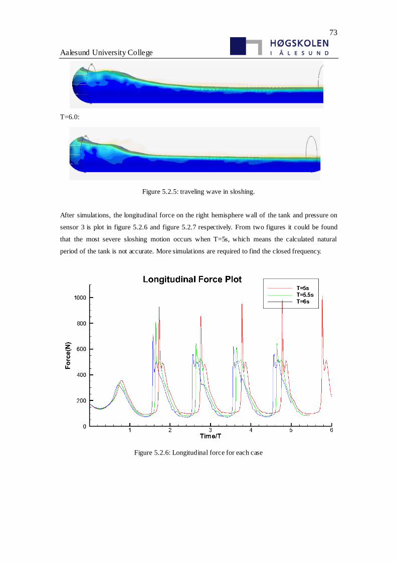
73
Aalesund University College
T=6.0:
Figure 5.2.5: traveling wave in sloshing.
After simulations, the longitudinal force on the right hemisphere wall of the tank and pressure on
sensor 3 is plot in figure 5.2.6 and figure 5.2.7 respectively. From two figures it could be found
that the most severe sloshing motion occurs when T=5s, which means the calculated natural
period of the tank is not accurate. More simulations are required to find the closed frequency.
Figure 5.2.6: Longitudinal force for each case
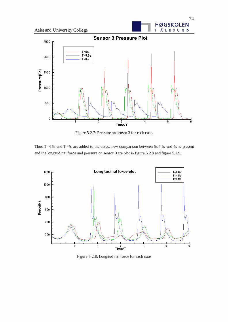
74
Aalesund University College
Figure 5.2.7: Pressure on sensor 3 for each case.
Thus T=4.5s and T=4s are added to the cases: new comparison between 5s,4.5s and 4s is present
and the longitudinal force and pressure on sensor 3 are plot in figure 5.2.8 and figure 5.2.9.
Figure 5.2.8: Longitudinal force for each case
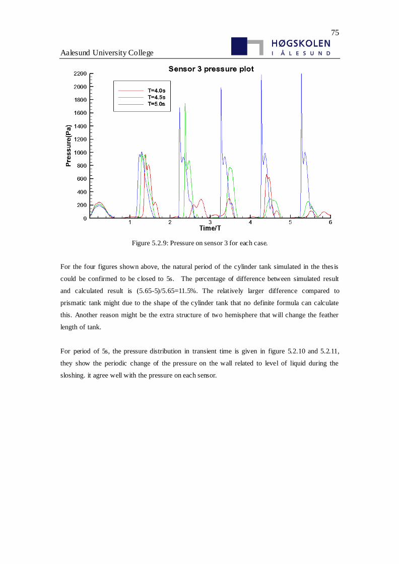
75
Aalesund University College
Figure 5.2.9: Pressure on sensor 3 for each case.
For the four figures shown above, the natural period of the cylinder tank simulated in the thes is
could be confirmed to be closed to 5s. The percentage of difference between simulated result
and calculated result is (5.65-5)/5.65=11.5%. The relatively larger difference compared to
prismatic tank might due to the shape of the cylinder tank that no definite formula can calculate
this. Another reason might be the extra structure of two hemisphere that will change the feather
length of tank.
For period of 5s, the pressure distribution in transient time is given in figure 5.2.10 and 5.2.11,
they show the periodic change of the pressure on the wall related to level of liquid during the
sloshing. it agree well with the pressure on each sensor.
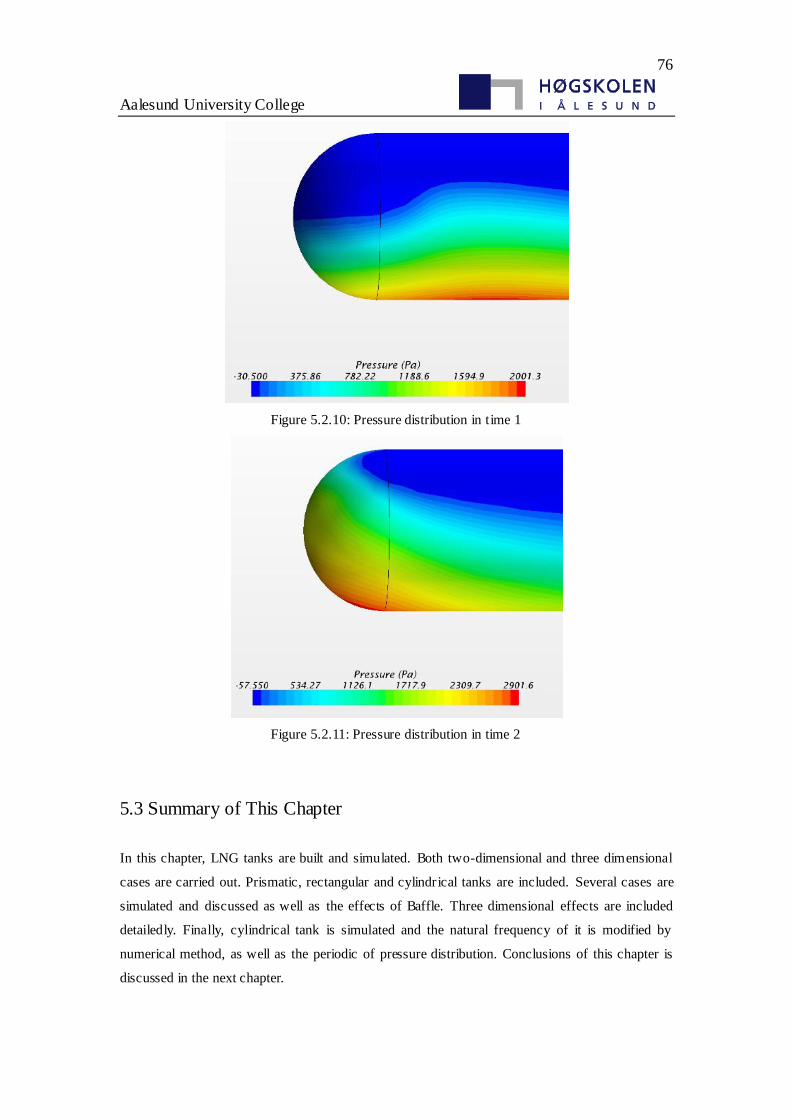
76
Aalesund University College
Figure 5.2.10: Pressure distribution in time 1
Figure 5.2.11: Pressure distribution in time 2
5.3 Summary of This Chapter
In this chapter, LNG tanks are built and simulated. Both two-dimensional and three dimensional
cases are carried out. Prismatic, rectangular and cylindrical tanks are included. Several cases are
simulated and discussed as well as the effects of Baffle. Three dimensional effects are included
detailedly. Finally, cylindrical tank is simulated and the natural frequency of it is modified by
numerical method, as well as the periodic of pressure distribution. Conclusions of this chapter is
discussed in the next chapter.
77
Aalesund University College
6.Summary
6.1.Conclusion
This thesis mainly deals with the sloshing problem of LNG tanks. The types of tanks contain
prismatic, rectangular and cylindrical tanks. A large amount of model is involved and simulated in
STAR-CCM+ to get the movement and shape of free surface, hydrodynamic force and pressure of
the sloshing motion. Conclusion of this thesis consist of two main part:
The current numerical methods is validated by a published experimental result and shows a good
agreement with the experimental results before impact load and a acceptable agreement with that
after impact load. The natural frequency of prismatic tank and rectangular tank calculated by
empirical formula and numerical method agree well with each other. The percentage of
difference are (4.6% and5.5% respectively for prismatic and rectangular tank in transverse and
longitudinal direction. Besides, amplitude of tank motion could influence the severity of sloshing
motion signif icantly. Finally, three dimensional effect is existing in simulation of 3-D model that
longitudinal oscillation occurs with transverse tank motion.
A lower liquid filling level could induce a larger impact pressure in the same tank motion for
Prismatic LNG tank in longitudinal direction. The increase of the liquid depth will increase the
nonlinearity of the liquid motion. At 50% and 70% liquid fillings, the wave breaking and liquid
splashing phenomenon could be eas ily observed. For the effects of baffle, T=1.2s is closed to
natural period of the prismatic tank with baffle mostly. The impact pressure for cases with baffle
decrease significantly comparing with that on the non-baffle cases. For sway motion, the
percentage of reduction is77.4% while for pitch motion the percentage could be 83.3%. The
increase of number of baffle can reduce the pressure, or sloshing motion signif icantly.
Although the tank motion is only in transverse direction, sloshing motion in longitudinal direction
is also existing. surge motion do influence the pressure distribution but not much, which means
the longitudinal sloshing motion that may cause resonance oscillation has little effects on
transverse direction.
the natural period of the cylinder tank simulated in the thesis is closed to 5s. The percentage of
difference between simulated result and calculated result is 11.5%. The relatively larger difference
compared to prismatic tank might due to the shape of the cylinder tank that no definite formula
can calculate this. Another reason might be the extra structure of two hemisphere that will change
78
Aalesund University College
the feather length of tank. Pressure distribution on the wall is periodic and agree well with the
results on sensor.
6.2.Shortage
Shortage of the thesis contain five parts. Firstly, due to the limit of time and tools, the basic size of
mesh cells is set to an acceptable value both for time memory saving. To get more accurate results,
the basic size could be smaller. And the time step could also be smaller to be more converged.
Secondly, tank models built in this thesis are always simplified models. Some of them only
contain a baffle. In reality, there are more complex inner structures such as the pipe system that
will influence the sloshing. Thirdly, Interaction between tank wall and liquid is not included. The
tank wall in this thesis is set to be rigid body, which, however, in reality it has elastics. Then
hydroelastic should be considered. Besides, LNG defined in STAR-CCM+ is a definite liquid with
constant physical properties. But in reality LNG contains several components, which comes to the
last shortage, the heat transfer and phase change in sloshing. This will be moved to Appendix B
6.3.Future work
Future work should focus on the optimization of model, both for the arrangement of tank and
setting in software. More kinds of tanks and more complex movement could be involved.
Temperature of the model and phase changes could be considered. At last, I am really interested in
the hydroelastic. In the future, maybe the study of me will mainly focus on it.
79
Aalesund University College
7.Reference
[1]Moiseyev N N. To the theory of nonlinear oscillations of a limited liquid volume of a liquid[J].
Prikl. Math. Mech, 1958, 22: 612-621.
[2]Abramson H N. The dynamic behavior of liquids in moving containers, with applications to
space vehicle technology[J]. 1966.
[3]Solaas F, Faltinsen O M. Combined numerical and analytical solution for sloshing in
two-dimensional tanks of general shape[J]. Journal of ship research, 1997, 41(2): 118-129.
[4]Faltinsen O M, Timokha A N. An adaptive multimodal approach to nonlinear sloshing in a
rectangular tank[J]. Journal of Fluid Mechanics, 2001, 432: 167-200.
[5]W. J. Rider and D. B. Kothe. Reconstructing volume tracking. Journal of Computational
Physics. 1998(141):112–152
[6]Harlow F H, Welch J E. Numerical calculation of time-dependent viscous incompressible flow
of fluid with free surface[J]. Physics of fluids, 1965, 8(12): 2182.
[7]Feng, G.C., 1973. Dynamic loads due to moving liquid. AIAA Paper No. 73-409
[8]C.W. Hirt, B.D. Nichols Volume of fluid method for the dynamics of free boundaries J. Comput.
Phys. 1981(39): 201–225.
[9]Solaas F. Analytical and numerical studies of sloshing in tanks[D]. Norwegian Institute of
Technology, 1995.
[10]Rudman M. Volume-tracking methods for interfacial flow calculations[J]. International
journal for numerical methods in fluids, 1997, 24(7): 671-691.
[11]Van Daalen E F G, Kleefsman K M T, Gerrits J, et al. Anti Roll Tank Simulations with a
Volume Of Fluid (VOF) based Navier-Stokes Solver[C]23rd. Symposium on Naval
Hydrodynamics. 2000.
[12]Kim Y. Numerical Simulation of Sloshing Flows with Impact Load[J].Applied Ocean
Reasarch,2001(23):53-62.
[13]Celebi M S, Akyildiz H. Nonlinear modeling of liquid sloshing in a moving rectangular
tank[J]. Ocean Engineering,2002(29):1527-1553.
[14]Akyildiz H. Sloshing in a three-dimensional rectangular tank-Numerical simulation and
experimental validation[J].Ocean Engineering,2006(23):2135-2149.
[15]Liu Dongming, Lin Pengzhi. A numerical study of three dimensional liquid sloshing in
tanks[J]. Journal of Computational Physics,2008(227):3921-3939.
[16]Ramaswamy B, Kawahara M. Arbitrary Lagrangian–Eulerianc finite element method for
unsteady, convective, incompressible viscous free surface fluid flow[J]. International Journal for
Numerical Methods in Fluids, 1987, 7(10): 1053-1075.
[17]Okamoto T, Kawahara M. Two‐dimensional sloshing analysis by Lagrangian finite element
method[J]. International Journal for Numerical Methods in Fluids, 1990, 11(5): 453-477.
80
Aalesund University College
[18]Mashayek F, Ashgriz N. A hybrid finite‐element–volume‐of‐fluid method for simulating
free surface flows and interfaces[J]. International journal for numerical methods in fluids, 1995,
20(12): 1363-1380.
[19]Ma Q W, Wu G X, Taylor R E. Numerical simulation of sloshing waves in a 3D
tank[C]//Proceedings 13th International Workshop on Water Waves and Floating Bodies : 29
March-1 April 1998 Alphen Aan Den Rijn, the Netherlands. Delft Univ Pr, 1998: 87.
[20]Brebbia C A. Boundary element methods in engineering[M]. New York: Springer, 1982.
[21]Gingold R A, Monaghan J J. Smoothed particle hydrodynamics: theory and application to
non-spherical stars[J]. Monthly notices of the royal astronomical society, 1977, 181(3): 375-389.
[22]Akyildiz H. Experimental investigation of pressure distribution on a rectangular tank due to
the liquid sloshing[J].Ocean Engineering,2005(32):1503-1516.
[23]Nasar T. Experimental study of liquid sloshing dynamics in a barge carrying tank[J].Fluid
Dyamics Research,2008(40):427-458.
[24]Kim Y. Experimental and numerical analyses of sloshing flows[J]. Journal of Engineering
Mathematics, 2007, 58(1-4): 191-210.
[25]Khezzar L, Seibi A, Goharzadeh A. Water Sloshing in Rectangular Tanks–An Experimental
Investigation & Numerical Simulation[J]. International Journal of Engineering (IJE), 2009, 3(2):
174.
[26] Faltinsen, O.M., Timokha, A.N. Sloshing. 2009.
[27] Yang C, Löhner R. Computation of 3D flows with violent free surface motion[J]. Proc. 15th
ISOPE, 2005.
[28] Näslund M. LNG-Status in Denmark[J]. Technology and potential. Project report. Danish
Gas Technology Centre. 2012(12): 2013.
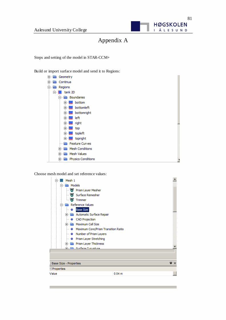
81
Aalesund University College
Appendix A
Steps and setting of the model in STAR-CCM+
Build or import surface model and send it to Regions:
Choose mesh model and set reference values:
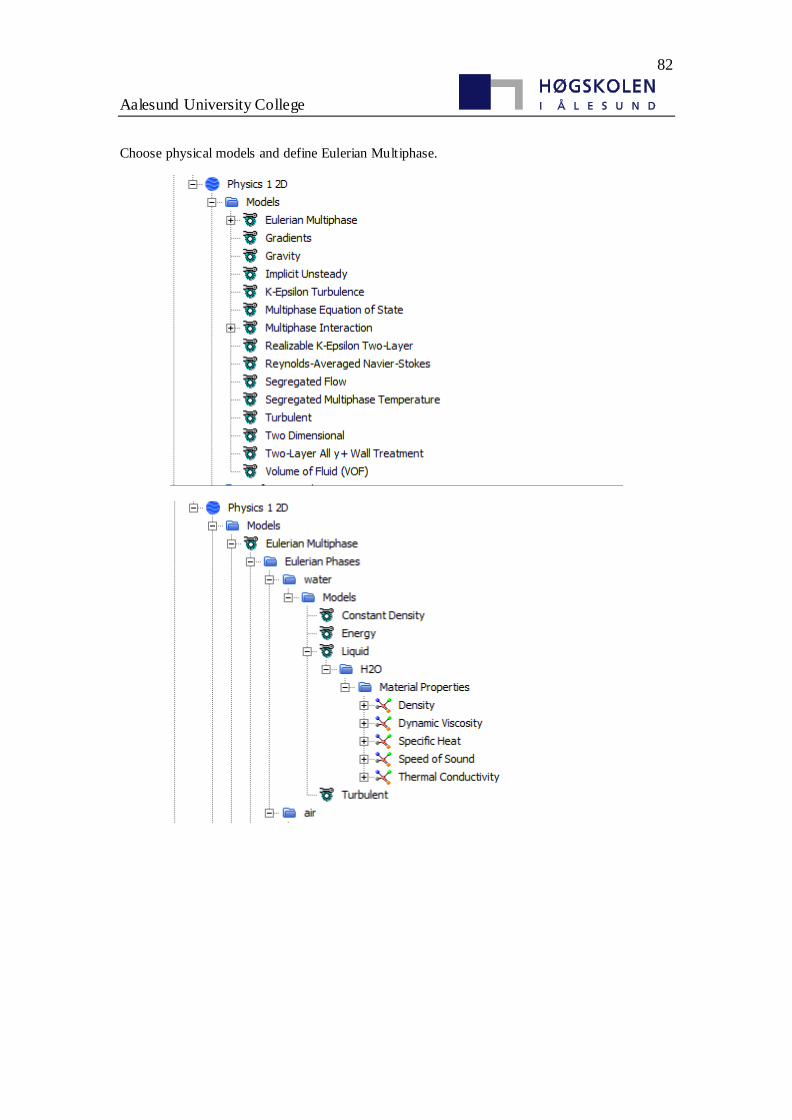
82
Aalesund University College
Choose physical models and define Eulerian Multiphase.
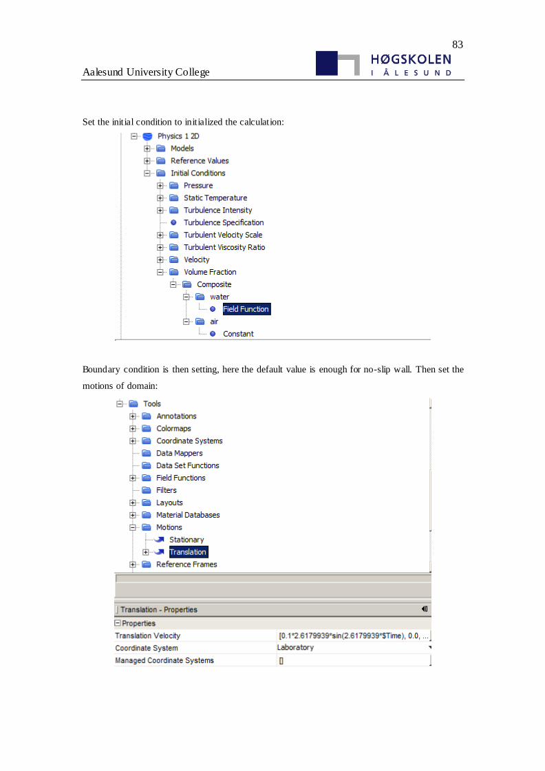
83
Aalesund University College
Set the initial condition to initialized the calculation:
Boundary condition is then setting, here the default value is enough for no-slip wall. Then set the
motions of domain:
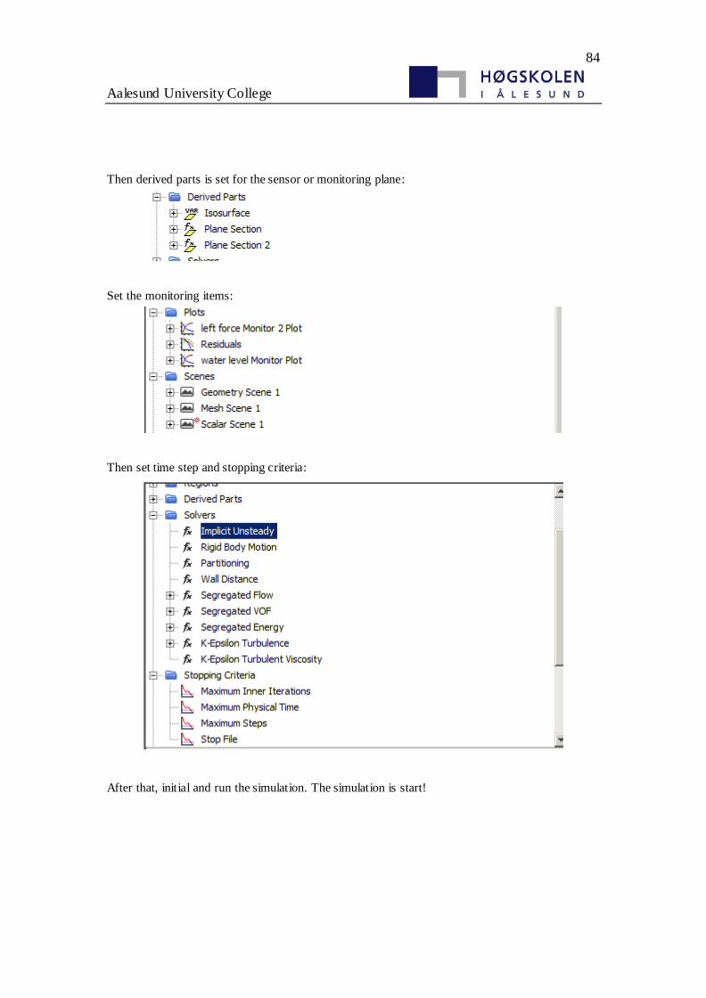
84
Aalesund University College
Then derived parts is set for the sensor or monitoring plane:
Set the monitoring items:
Then set time step and stopping criteria:
After that, initial and run the simulation. The simulation is start!
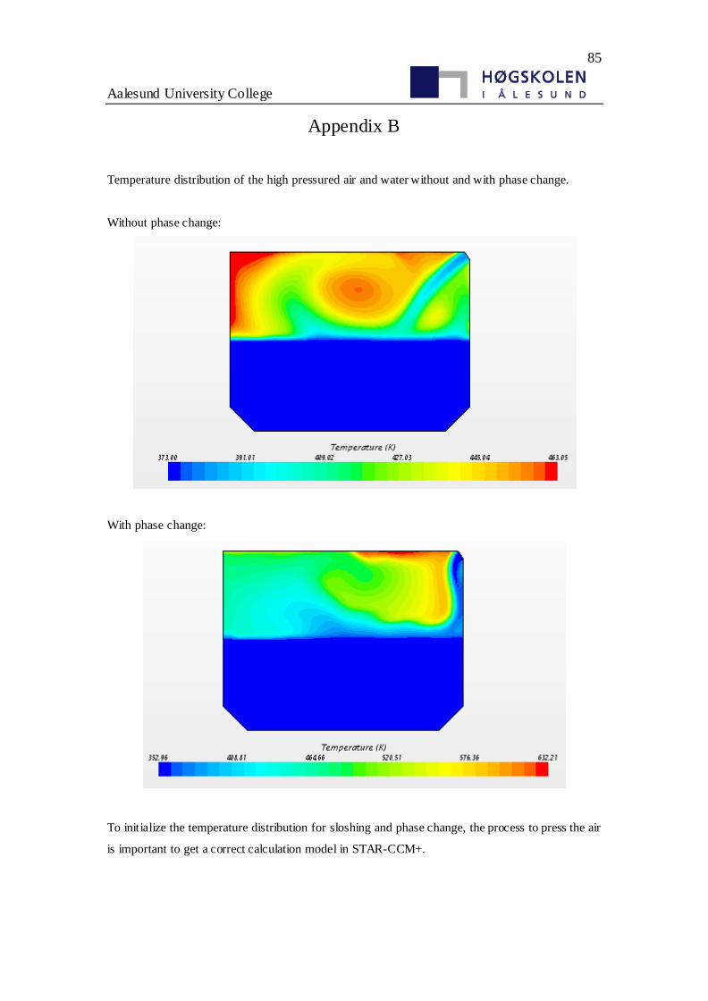
85
Aalesund University College
Appendix B
Temperature distribution of the high pressured air and water without and with phase change.
Without phase change:
With phase change:
To initialize the temperature distribution for sloshing and phase change, the process to press the air
is important to get a correct calculation model in STAR-CCM+.