Modeling biological systems using Dynetica – a simulator of

dynamic networks

June 2002

Lingchong You 1, Apirak Hoonlor 2, and John Yin 3*

1Division of Chemistry and Chemical Engineering, California Institute of Technology

2Department of Computer Sciences, University of Wisconsin-Madison

3Department of Chemical Engineering, University of Wisconsin-Madison

Running title: Dynetica – a simulator of dynamic networks

Keywords: mathematical modeling, deterministic simulation, stochastic simulation,

genetic network.

* To whom correspondence should be addressed: Department of Chemical Engineering, University of Wisconsin-Madison, 1415 Engineering Drive, Madison, WI 53706, USA. Email: yin@engr.wisc.edu.

ABSTRACT

Mathematical modeling and computer simulation may deepen our understanding

of complex systems by testing the validity and consistency of experimental data and

mechanisms, by generating experimentally testable hypotheses, and by providing new

insight into the integrated behaviors of these systems. However, the application of this

approach in biology has been hindered by the lack of software tools to build and analyze

models. To meet this need, we have developed Dynetica – a simulator of dynamic

networks – to facilitate model building for systems that can be expressed as reaction

networks. A distinguishing feature of Dynetica is that it facilitates easy construction of

models for genetic networks, where many reactions are the expression of genes and the

interactions among gene products. In addition, it provides users the flexibility of

performing time-course simulations using either deterministic or stochastic algorithms.

Finally, since it is written in Java, Dynetica is platform-independent, allowing models to

be easily shared among researchers. We anticipate that Dynetica will dramatically speed

up the process of model construction and analysis for a wide variety of biological

systems.

Availability: Dynetica 1.0 and the example models are freely available on request.

Contact: you@cheme.caltech.edu

2

INTRODUCTION

Over the past several decades, mathematical modeling has arguably become an

important tool in biological research. Owing to the lack of detailed information for many

biological systems, past efforts in modeling have relied on relatively simple approaches,

such as Boolean network modeling (Glass and Kauffman 1973; Thomas 1973; Glass

1975) and stoichiometric modeling (Clarke 1988; Fell 1992). In Boolean representations

of gene networks, each gene is treated as having two states, ON or OFF, and the

dynamics describes how genes interact to change one another’s states over time (Hasty et

al. 2001). Although a Boolean model can provide insight into the qualitative behavior of

the underlying system, it is usually overly simplified and tends to give ambiguous

predictions (Kuipers 1986). A stoichiometric model represents the underlying system as a

series of coupled chemical reactions. It does not require any information on the kinetics

of the reactions, and as such is particularly attractive for systems where only sparse

kinetic data are available or when steady-state assumptions can be justified (Varner and

Ramkrishna 1999; Bailey 2001). Coupled with a technique called metabolic flux analysis

(Fell 1992), stoichiometric models have played an instrumental role in shaping the field

of metabolic engineering, by providing theoretic guidance for experimental manipulation

of metabolic networks (Stephanopoulos et al. 1998). Recently, stoichiometric models

have proven powerful in characterizing the underlying structure of metabolic networks by

determining the elementary flux modes (Schuster et al. 2000) or the null space base

vectors (Schilling and Palsson 1998) and in predicting steady-state metabolic capabilities

of several model organisms, such as E. coli (Schilling et al. 1999; Edwards et al. 2001)

3

and H. influenzae (Edwards and Palsson 1999). But their applications are limited by their

inability to predict the temporal evolution of these networks. To make such predictions,

the stoichiometric structure of the reaction networks needs be supplemented with detailed

kinetic information, resulting in kinetic models. Thanks to the rapid expansion of our

knowledge in biology, kinetic modeling has become a realistic goal, particularly for the

experimentally well-characterized systems. For example, kinetic models have recently

been successfully applied to the analysis of a wide variety of biological systems,

including bacterial chemotaxis signaling networks (Barkai and Leibler 1997; Spiro et al.

1997), developmental pattern formation in Drosophila (Reinitz et al. 1998; von Dassow

et al. 2000), aggregation stage network of Dictyostelium (Laub and Loomis 1998), viral

infection (Shea and Ackers 1985; Eigen et al. 1991; McAdams and Shapiro 1995; Endy

et al. 1997; Reddy and Yin 1999; You et al. 2002), circadian rhythms (Barkai and Leibler

2000; Smolen et al. 2001), single cell growth (Shuler et al. 1979), and physiological

processes (Quick and Shuler 1999; Winslow et al. 2000; Noble 2002).

A kinetic model essentially represents a mathematical integration of existing data

and mechanisms on a particular system, and may be useful in a number of ways. By

providing a global view of the underlying system, a kinetic model can be used to test the

consistency in the experimental data or mechanisms (von Dassow et al. 2000) or provide

mechanistic explanations for counter-intuitive observations (Fallon and Lauffenburger

2000), to facilitate the formulation of experimentally testable hypotheses (Abouhamad et

al. 1998; Endy et al. 2000; You et al. 2002) or to test hypotheses that are difficult,

expensive, or even impossible to explore experimentally with current technology (You

and Yin 2002), and to provide insight into emergent properties, such as robustness

(Barkai and Leibler 1997; Alon et al. 1999; von Dassow et al. 2000), which may be

4

otherwise difficult to grasp intuitively. As models become more “realistic” by

incorporating more detailed data and mechanisms, they may be treated as in silico

organisms and used to explore applied or fundamental questions that are beyond the

underlying system per se. For example, a phage T7 model has been employed to explore

anti-viral strategies using anti-sense mRNAs (Endy and Yin 2000), to elucidate the nature

of genetic interactions by in silico mutagenesis at the population level (You and Yin

2002), and to test data-mining strategies for identifying potential protein-protein

interactions from gene expression data (You and Yin 2000). Moreover, advances in high-

throughput biotechnologies for genome-wide gene expression profiling at the

transcription and translation level provide additional challenges and opportunities for

mathematical modeling, which may accelerate the characterization of whole organisms

by allowing the understanding of gene expression data (at the mRNA level or the protein

level) in their natural context.

formulation of DNA microarray data was used to determine the timing of transcriptional

onsets and cessation in Dictyostelium (Iranfar et al. 2001).

Despite its potential benefits for fundamental and applied biological research,

broader application of kinetic modeling has been hindered by the lack of powerful and

easy-to-use software tools for model construction and analysis. This is particularly true

for experimental biologists who are often unfamiliar with numerical methods and

programming. This aspect is probably best evidenced by the fact that the majority of

mathematical models of biological systems have been developed by researchers trained in

disciplines other than biology. Further, because of the lack of such tools, most published

models were developed from scratch, which can be a tedious and error-prone process.

This point is demonstrated in a recent work where kinetic

5

To address this issue, a number of programs that aim to facilitate the model

construction and analysis have been developed in the last several years. These programs

include Gepasi (Mendes 1993; Mendes 1997), DBsolve (Goryanin et al. 1999), E-Cell

(Tomita et al. 1999; Tomita 2001), SCAMP (Sauro 1993), STELLA, Virtual Cell (Schaff

et al. 1997; Schaff and Loew 1999; Schaff et al. 2000), StochSim (Morton-Firth and Bray

1998), and STOCKS (Kierzek 2002). It would go beyond the scope of this current work

to give a detailed account of these tools. Briefly, Gepasi, DBsolve, and SCAMP focus on

the analysis of biochemical and metabolic networks. In addition to basic time-course

simulations, these programs provide additional modules to explore the properties of

metabolic networks. E-Cell aims to construct whole-cell models, and it has been applied

to model a self-sustaining hypothetic cell (Tomita et al. 1999) and a human erythrocyte

(Tomita 2001). Virtual Cell is advantageous in that it accounts for the diffusion of

molecules in addition to their reactions in describing cellular processes. Distinct from

other programs, StochSim and STOCKS simulate the system dynamics using stochastic

algorithms instead of deterministic algorithms. These two differ in that StochSim

employs a semi-empirical algorithm, while STOCKS uses the Gillespie algorithm

(Gillespie 1977), which is rigorous for spatially homogenous systems. More extensive

discussion of recent progress in the development of modeling tools may be found in

excellent recent reviews (Arkin 2001; Loew and Schaff 2001).

We present here a unique, general-purpose computational framework for creating,

visualizing, and analyzing mathematical models of biological networks, including

biochemical, metabolic, signaling, and genetic networks. We call this program Dynetica,

or a simulator of dynamic networks. Dynetica is distinct from other software packages in

6

three aspects: (1) it facilitates the construction of kinetic models of genetic networks

where most reactions are expression of genes; (2) it provides a visual representation of

each model for interactive manipulation and interrogation; (3) it allows time-course

simulations using both deterministic and stochastic algorithms. Furthermore, because it is

written in Java, a platform-independent, object-oriented programming language, Dynetica

can be run on most modern computers, which will facilitate the sharing of models among

researchers. We anticipate that Dynetica will contribute significantly to advancing

broader application of kinetic modeling in biological systems.

MODELING IN DYNETICA

Representation of generic reaction networks

A reaction network in Dynetica consists of a list of substances that interact with

one another via a list of reactions. Kinetics of these reactions may be specified by a list of

parameters (Figure 1). In addition to a tree structure, Dynetica provides a graphic

representation of each reaction network. Figure 2 shows a hypothetical reaction network

in Dynetica that consists of two reactions (Table 1). Each reaction is characterized by two

basic attributes: its stoichiometry, which specifies the quantitative relationship between

the substances in a reaction, and its kinetics, which specifies how fast (for non-

equilibrated reactions) or to what extent (for equilibrated reactions) the reaction occurs.

Dynetica employs two modules to describe generic reaction networks: a reaction

parser and a mathematical expression parser. The reaction parser can interpret

7

conventional chemical reaction formulas (using “→” as the separator between reactants

and products), which specify the stoichiometry of reactions. The mathematical expression

parser is used to interpret conventional mathematical expressions, which describe the

kinetics of reactions. In Dynetica expressions both substances and parameters have values

associated with them. The expression parser distinguishes between these entities by

enclosing substance names with brackets. For example, the rate expression for reaction

R1 in Table 1 is k1 [A] [E], which means the value of parameter k1 times the level of

substance A and the level of substance E. The expression parser can interpret

mathematical expressions composed of the operations and functions shown in Table 2.

The kinetics of most chemical reactions can be formulated easily within this framework.

Representation of genetic networks

Genetic networks can be loosely defined as reaction networks involving gene

expression processes, such as transcription of genes and translation of mRNAs. In

Dynetica, a genetic network is treated as a special reaction network that contains one or

more genomes (Figure 3A). Here a genome is defined as an entity composed of an array

of genetic elements, such as genes, promoters, and transcription terminators. Examples of

genomes include genomes of cells and viruses, as well as plasmids.

Each genetic element is characterized by two attributes, namely, its starting and

ending positions (in base-pair number) along the genome. A gene in Dynetica is a special

genetic element characterized by several additional attributes: the RNA polymerase

responsible for its transcription, the ribosome responsible for its translation, the name of

its RNA, and the name of its protein (if the gene is to be translated), the relative

transcription activity, and the relative translation activity. The relative transcription

8

activity is essentially a weighting factor by which RNA polymerases are allocated to

different genes, and the relative translation activity is the weighting factor by which

ribosomes are allocated to different genes (more precisely, to different mRNAs). Genetic

reactions can easily be formulated in Dynetica. Figure 3B demonstrates the Dynetica

formulation of the central dogma of molecular biology. Essentially, the information

transfer process from gene to mRNA to protein can be represented by two reactions. The

transcription reaction specifies the conversion of nucleoside triphosphates (NTP) into

mRNA, and is catalyzed by the gene and RNA polymerase (RNAP). The translation

reaction specifies the conversion of amino acids (AA) into the protein, and is catalyzed

by the mRNA and the ribosome.

Because expression of most genes follows the pattern as specified by the central

dogma, Dynetica automatically creates a transcription reaction and a translation reaction

for each gene that the user specifies in a genome. In addition, it also generates two

reactions to represent the degradation of the gene products, the mRNA and the protein. In

setting up the transcription reaction, we assume that the limiting step is the elongation of

the RNAP, and the transcription follows Michaelis-Menten kinetics with NTP as the

substrate. For the translation reaction, we assume that the limiting step is the elongation

of the ribosome, and the reaction follows Michaelis-Menten kinetics with AA as the

substrate. Note that these automatically generated reactions are essentially “first-order

approximations” by the program based on the genetic information provided by the user.

These approximations are useful because they provide an initial estimate of gene

expression dynamics. The user can then refine the stoichiometry and kinetics of such

reactions as needed.

9

Simulation

A model in Dynetica gives a schematic representation of the corresponding

system, but it does not specify how the system evolves over time. The latter will be

determined by an algorithm. Here, an algorithm is defined as the scheme by which the

system represented by the model will be updated as a function of time. It can be either

deterministic or stochastic. Deterministic algorithms include all the traditional numerical

algorithms that are designed to solve coupled differential equations, such as fixed or

variable time-step Runge-Kutta algorithms. A deterministic algorithm is appropriate

when the continuity of the system can be justified.

Stochastic algorithms focus on updating reactions in the system. For example, a

widely used stochastic algorithm proposed by Gillespie (Gillespie 1977) updates a

reactive system by determining, at each step, which and when the next reaction will

occur. A stochastic algorithm is appropriate for a spatially homogeneous system where

the interacting molecules are few that fluctuations in their numbers are significant. A

number of researchers have strongly advocated the use of stochastic algorithms for

modeling biological systems, especially for intracellular processes (Arkin et al. 1998;

Goss and Peccoud 1998; Morton-Firth and Bray 1998; Kierzek 2002).

The structure of a reaction network model in Dynetica is flexible enough to allow

simulations by either deterministic or stochastic algorithms. Currently we have

implemented three different algorithms: a fixed time-step 4th order Runge-Kutta

algorithm, a variable time-step 4th order Runge-Kutta algorithm, and Gillespie’s

algorithm. By applying an algorithm to a model, we can generate the dynamics of the

underlying system. Shown in Figure 4 are the results of deterministic and stochastic

10

simulations with the model in Figure 2. In this particular case, both approaches generate

qualitatively the same result: substance A is gradually converted into substance B until

equilibrium is reached, whereas the level of substance E remains constant over time.

However, the details of the dynamics generated from these different approaches are quite

different. For instance, there are no fluctuations in the substance concentrations as

predicted by the deterministic simulation, but fluctuations are evident in the result from

the stochastic simulation. In addition, because of the stochastic aspect of the Gillespie

algorithm, every new simulation starting from the same initial condition will generate

different dynamics (Gillespie 1977).

In addition to simulating the temporal evolution of a reaction network, Dynetica

provides the basic functionality to explore how the dynamics of the network responds to

the perturbations to the network, in terms of variations in parameter values or the initial

levels of substances. This feature is desirable for simulating dosage curves and for

identifying key system parameters that are important in determining overall behaviors of

the system.

APPLICATIONS

To demonstrate the application of Dynetica we use it to build two models: one for

the Dictyostelium aggregation stage network, and the other for the intracellular growth

cycle of phage T7. The aggregation stage network model is shown here as an example of

a general reaction network. The phage T7 model shown as an example of a genetic

network.

11

A Dictyostelium aggregation stage network model

Amoebae of Dictyostelium discoideum grow as independent cells in the soil, but

aggregate and develop as a multicellular organism under starvation. It has been proposed

that the aggregation stage network, which consists of seven interacting components, is

responsible for regulating the expression of developmental genes in homogeneous

populations of Dictyostelium shortly after starvation (Loomis 1998; Soderbom and

Loomis 1998). Previously, a kinetic model was developed to analyze the dynamics of this

signaling network (Laub and Loomis 1998). The model accounted for the interactions

among seven molecular species, and was shown to be able to predict the oscillations in

the enzyme activities during Dictyostelium development.

Based on (Laub and Loomis 1998), we used Dynetica to reconstruct the

aggregation stage network model (Figure 5A, Table 3). Figure 5B shows a representative

simulation result demonstrating stable oscillations in levels of the interacting

components.

A phage T7 model

Phage T7 is a lytic virus that infects bacterium E. coli. By incorporating the

existing experimental data and mechanisms of T7 biology, we previously developed a

genetically structured kinetic model to account for the intracellular life cycle of phage T7

(Endy et al. 1997; Endy et al. 2000; You et al. 2002). Various versions of this model were

employed to explore anti-viral strategies (Endy et al. 1997; Endy and Yin 2000), effects

of host physiology on phage development (You et al. 2002), design principles of phage

T7 (Endy et al. 2000; You and Yin 2001), genetic interactions among deleterious

12

mutations (You and Yin 2002), and data-mining strategies for identifying potential

protein-protein interactions from gene expression data (You and Yin 2000).

The model presented here is a simplified version of the previous models (Figure

6). The major difference between the current model and the previous ones is that a

simplified genome is used here (Figure 6A). This simplified genome contains 20 essential

T7 genes. The regulatory effect of promoters and transcription terminators is accounted

for by specifying the relative transcription activity of each gene. As a result, RNA

polymerases are allocated to different genes based on their relative transcription

activities, whereas in the complete model RNA polymerases are allocated based on the

relative strengths of promoters (You et al. 2002). The resulting T7 reaction network

contains 91 reactions and 55 substances, excluding genes (Figure 6B). In this network,

the reactions describing expression of genes and degradation of gene products are

automatically generated by Dynetica. Although the network diagram is overall complex,

it highlights several features of the system. First, most substances are involved in two

reactions, one for production (green line) and the other for consumption (red line).

Second, several nodes (as labeled) are highly connected. For example, the nodes for

amino acid and NTP are highly connected because these two substances are used as

precursors for transcription and translation reactions, respectively. Likewise, the nodes

for T7 RNAP and ribosome are highly connected because they are used as catalysts for

transcription and translation reactions, respectively.

Like the more comprehensive model, the current model accounts for the major

steps of T7 infection: transcription of viral genes, translation of the resulting mRNAs,

interactions between regulatory proteins, host DNA degradation and T7 DNA replication,

13

procapsid assembly, and eventually production of phage progeny. A representative

simulation result showing the time courses of three viral components is presented in

Figure 6c. It illustrates the synthesis of T7 DNAs and procapsids, and the packaging of

T7 DNAs into procapsids to form viral progeny. Overall, this simplified model captures

the main features of viral growth as predicted by the more comprehensive model.

DISCUSSION

We have developed Dynetica to facilitate the construction, visualization and

analysis of mathematical models for biological systems that can be formulated as a

coupled system of reactions. With Dynetica, the user need only specify the chemistry of

this system, that is, what components are in the system and how they interact.

Throughout the model-building process, the user need not write any differential

equations, or formulate numerical algorithms to conduct simulations. Instead, the

numerics is automatically handled by the program. Thanks to this feature, the user can

focus on the model itself and its practical relevance rather than the technical aspects of

computer simulation. Furthermore, by providing a graphic view of the underlying

reaction network Dynetica will facilitate the interactive manipulation and analysis of each

model.

Dynetica’s ability to perform both deterministic and stochastic simulations on the

same model may facilitate comparative studies of these two approaches. Deterministic

algorithms have been traditionally used to simulate the dynamics of a system of coupled

reaction network. However, the small numbers of interacting components in some

intracellular processes may become an issue. First, the continuity of these systems is no

14

longer warranted. Second, fluctuations in the concentrations of the reacting components

may significantly impact the system dynamics. Because of these issues, some researchers

have questioned the use of deterministic algorithms in simulating the behaviors of

biological systems, and suggested using stochastic algorithms instead (Arkin et al. 1998;

Goss and Peccoud 1998; Morton-Firth and Bray 1998; Kierzek 2002). They have shown

that stochastic simulations often produce dynamics drastically different from what is

predicted by deterministic simulations. Moreover, they have argued that a stochastic

simulation more accurately and more completely accounts for the temporal evolution of a

well-stirred chemical reaction network than does a deterministic algorithm (Gillespie

1977; McAdams and Arkin 1998). Nonetheless, since a stochastic algorithm only gives

accurate solutions for a well-stirred system, it may not be applicable for intracellular

processes. It is unclear whether it is more appropriate than a deterministic approach in

modeling such processes. To this end, Dynetica may be employed to simulate a system

using both deterministic and stochastic approaches and explore which approach is more

appropriate in a particular situation.

With its present underlying software structure, Dynetica can easily be extended in

its functionality and flexibility. It has a software module that automates the construction

of a genetic network model based on the organization of genetic elements along the

genome. In achieving this functionality, we made simplifying assumptions regarding the

organization of the genome. For each gene, Dynetica will automatically generate a

transcription reaction, a translation reaction, and degradation reactions for the resulting

mRNA and protein. However, in reality, there are also genes for tRNA and rRNA that do

not have protein products. Future modifications of the program will be needed to

represent and distinguish different kinds of genes. New numerical algorithms can be

15

implemented, so that the user will have the freedom in choosing the most appropriate one

for a given situation. Further, we are developing model templates for different types of

biological systems, such as signaling pathways, viruses, and single cells. Like the

document templates one may encounter in many word-processing programs such as

Microsoft® Word, these templates will further facilitate the model-building process,

particularly for new users. An emerging challenge for the modeling community lies in the

interchange of models constructed using different software tools, as listed in the

introduction section. Recently, there have been many efforts toward developing modeling

standards for biology modeling, such as the SBML (Systems Biology Markup Language)

project (http://www.cds.caltech.edu/erato) and the CellML (Cell Markup Language)

project (http://www.cellml.org). To provide exchangeable mathematical models, we plan

to implement software modules to import models constructed with other tools, or written

in standard modeling languages. Finally, we plan to implement software modules to

annotate models; we expect this functionality will further facilitate the communication of

mathematical models as a representation of the underlying biological systems.

The evolution of biological network modeling can be compared to that of the

molecular dynamics simulation, which uses physical principles to compute the structure

and dynamics of biological molecules. Although the development and use of molecular

dynamics simulation programs were initially much restricted to researchers with strong

background in theoretic physics and mathematics, it is the development of powerful and

user-friendly tools that has established this computational approach as a routine tool for

structural studies of natural or synthetic biological molecules (Loew and Schaff 2001).

Similarly we envision that, Dynetica, together with other emerging modeling tools, will

16

promote a broader application of mathematical models in cell biology by serving as a

computational platform to create, analyze and exchange such models.

ACKNOWLEDGMENTS

We thank Dr. William Loomis for clarifications on the aggregation stage network

model, and Yi-Fan Chen for technical assistance. Funding of this work was provided by

the National Science Foundation.

17

FIGURE LEGENDS

Figure 1. Representation of reaction networks in Dynetica. Each reaction network is

represented as three lists: substances, reactions through which substances interact with

one another, and parameters that specify the kinetics of the reactions.

Figure 2. Screenshot of a hypothetical reaction network in Dynetica. The left panel shows

the tree-structure view of the network, and the right panel gives a graphic representation.

In the graph a green line indicates the production of the connected substance by the

connected reaction, a red line represents the consumption of the connected substance by

the connected reaction, and a gray dashed line indicates that the connected substance

affects the kinetics of the connected reaction. See text for details of the reactions.

Figure 3. Formulation of genetic networks in Dynetica. (A) A genetic network in

Dynetica is represented as a special reaction network that contains one or more genomes.

(B) The central dogma represented in Dynetica.

Figure 4. The simulation results from the reaction network in Figure 2 using both (A)

deterministic and (B) stochastic algorithms.

Figure 5. Aggregation stage network model. (A) The graphic representation of the

reaction network. (B) A representative simulation result. The network was constructed

based on the reference (Laub and Loomis 1998). The reactions involved in this network

18

are shown in Table 3. The parameter values for the simulation are: k1 =1.4, k2 = 0.9, k3 =

2.5, k4 = 1.5, k5 = 0.6, k7 = 2.0, k8 = 1.3, k9 = 0.3, k10 = 0.8, k11 = 0.7, k12 = 4.9, k13 = 18,

k14 = 1.5 (W. Loomis, personal communication). The initial levels of all substances were

set to be 1.0, and the variable time-step 4th order Runge-Kutta algorithm was used for the

simulation.

Figure 6. Phage T7 model. (A) The simplified T7 genome. The left panel shows a list of

genes in the genome (not all genes are shown); the right panel shows the attributes of the

currently selected gene. (B) The graphic representation of the reaction network. The

reactions describing transcription and translation of genes were automatically generated

by Dynetica. (C) A representative simulation result showing the time courses of three

viral components.

19

Table 1. The reactions in the simple reaction network shown in Figure 2.

Reaction name Stoichiometry Kinetics

R1 A → B k1 [A] [E] a

R2 B → A k2 [B]

a The rate expression is actually written as k1 [A] * [E] in Dynetica.

20

Table 2. The mathematical operations and functions that are supported by Dynetica

Symbols or expressions Note

Basic operations +, -, *, /, ^ ‘^’ represents to the power of.

Basic functions a sin(a), cos(a), tan(a),

sqrt(a), log(a)

log(a) returns the natural logarithm

value of a

step(a, b) returns 1 if a ¥ b, and 0 otherwise

compare(a, b) returns 1 if a > b, 0 if a = b, and –1

if a < b

pulse(a, x, b) returns 1 if a < x < b, 0 otherwise

random(a, b) returns a random value between a

and b

rand() returns a random value between 0

and 1

min(a, b, c, …) returns the minimum value from

the list of arguments

Special functions a

max(a, b, c,…) returns the maximum value from

the list of arguments

a Each of the symbols (a, b, c and x ) may represent a simple variable or a mathematical

expression.

21

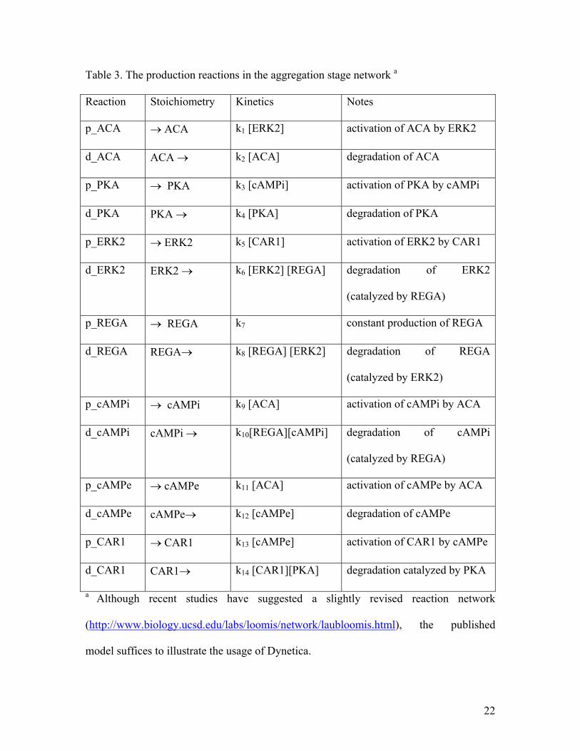
Table 3. The production reactions in the aggregation stage network a

Reaction Stoichiometry Kinetics Notes

p_ACA → ACA k1 [ERK2] activation of ACA by ERK2

d_ACA ACA → k2 [ACA] degradation of ACA

p_PKA → PKA k3 [cAMPi] activation of PKA by cAMPi

d_PKA PKA → k4 [PKA] degradation of PKA

p_ERK2 → ERK2 k5 [CAR1] activation of ERK2 by CAR1

d_ERK2 ERK2 → k6 [ERK2] [REGA] degradation of ERK2

(catalyzed by REGA)

p_REGA → REGA k7 constant production of REGA

d_REGA REGA→ k8 [REGA] [ERK2] degradation of REGA

(catalyzed by ERK2)

p_cAMPi → cAMPi k9 [ACA] activation of cAMPi by ACA

d_cAMPi cAMPi → k10[REGA][cAMPi] degradation of cAMPi

(catalyzed by REGA)

p_cAMPe → cAMPe k11 [ACA] activation of cAMPe by ACA

d_cAMPe cAMPe→ k12 [cAMPe] degradation of cAMPe

p_CAR1 → CAR1 k13 [cAMPe] activation of CAR1 by cAMPe

d_CAR1 CAR1→ k14 [CAR1][PKA] degradation catalyzed by PKA

a Although recent studies have suggested a slightly revised reaction network

(http://www.biology.ucsd.edu/labs/loomis/network/laubloomis.html), the published

model suffices to illustrate the usage of Dynetica.

22

REFERENCES

Abouhamad, W.N., D. Bray, M. Schuster, K.C. Boesch, R.E. Silversmith, and R.B.

Bourret. 1998. Computer-aided resolution of an experimental paradox in bacterial

chemotaxis. J Bacteriol 180: 3757-64.

Alon, U., M.G. Surette, N. Barkai, and S. Leibler. 1999. Robustness in bacterial

chemotaxis. Nature 397: 168-71.

Arkin, A., J. Ross, and H.H. McAdams. 1998. Stochastic kinetic analysis of

developmental pathway bifurcation in phage lambda-infected Escherichia coli

cells. Genetics 149: 1633-48.

Arkin, A.P. 2001. Synthetic cell biology. Curr Opin Biotechnol 12: 638-44.

Bailey, J.E. 2001. Complex biology with no parameters. Nat Biotechnol 19: 503-4.

Barkai, N. and S. Leibler. 1997. Robustness in simple biochemical networks. Nature 387:

913-7.

Barkai, N. and S. Leibler. 2000. Circadian clocks limited by noise. Nature 403: 267-8.

Clarke, B.L. 1988. Stoichiometric network analysis. Cell Biophys 12: 237-53.

Edwards, J.S., R.U. Ibarra, and B.O. Palsson. 2001. In silico predictions of Escherichia

coli metabolic capabilities are consistent with experimental data. Nat Biotechnol

19: 125-30.

Edwards, J.S. and B.O. Palsson. 1999. Systems properties of the Haemophilus influenzae

Rd metabolic genotype. J Biol Chem 274: 17410-6.

Eigen, M., C.K. Biebricher, M. Gebinoga, and W.C. Gardiner. 1991. The hypercycle.

Coupling of RNA and protein biosynthesis in the infection cycle of an RNA

23

bacteriophage. Biochemistry 30: 11005-11018.

Endy, D., D. Kong, and J. Yin. 1997. Intracellular kinetics of a growing virus: a

genetically structured simulation for bacteriophage T7. Biotech. Bioeng. 55: 375-

389.

Endy, D. and J. Yin. 2000. Toward antiviral strategies that resist viral escape. Antimicrob

Agents Chemother 44: 1097-9.

Endy, D., L. You, J. Yin, and I.J. Molineux. 2000. Computation, prediction, and

experimental tests of fitness for bacteriophage T7 mutants with permuted

genomes. Proc. Natl. Acad. Sci. U S A 97: 5375-5380.

Fallon, E.M. and D.A. Lauffenburger. 2000. Computational model for effects of

ligand/receptor binding properties on interleukin-2 trafficking dynamics and T

cell proliferation response. Biotechnol Prog 16: 905-16.

Fell, D.A. 1992. Metabolic control analysis: a survey of its theoretical and experimental

development. Biochem J 286: 313-30.

Gillespie, D.T. 1977. Exact stochastic simulation of coupled chemical reactions. J. Phys.

Chem. 81: 2340-2361.

Glass, L. 1975. Classification of biological networks by their qualitative dynamics. J.

Theor. Biol. 54: 85-107.

Glass, L. and S.A. Kauffman. 1973. The logical analysis of continuous, non-linear

biochemical control networks. J Theor Biol 39: 103-29.

Goryanin, I., T.C. Hodgman, and E. Selkov. 1999. Mathematical simulation and analysis

of cellular metabolism and regulation. Bioinformatics 15: 749-58.

24

Goss, P.J.E. and J. Peccoud. 1998. Quantitative modeling of stochastic systems in

molecular biology by using stochastic Petri nets. Proc. Natl. Acad. Sci. USA 95:

6750-6755.

Hasty, J., D. McMillen, F. Isaacs, and J.J. Collins. 2001. Computational studies of gene

regulatory networks: in numero molecular biology. Nat Rev Genet 2: 268-79.

Iranfar, N., D. Fuller, R. Sasik, T. Hwa, M. Laub, and W.F. Loomis. 2001. Expression

patterns of cell-type-specific genes in Dictyostelium. Mol Biol Cell 12: 2590-600.

Kierzek, A.M. 2002. STOCKS: STOChastic Kinetic Simulations of biochemical systems

with Gillespie algorithm. Bioinformatics 18: 470-81.

Kuipers, B. 1986. Qualitative Simulation. Artificial Intelligence 29: 289-338.

Laub, M.T. and W.F. Loomis. 1998. A molecular network that produces spontaneous

oscillations in excitable cells of Dictyostelium. Mol Biol Cell 9: 3521-32.

Loew, L.M. and J.C. Schaff. 2001. The Virtual Cell: a software environment for

computational cell biology. Trends Biotechnol 19: 401-6.

Loomis, W.F. 1998. Role of PKA in the timing of developmental events in Dictyostelium

cells. Microbiol Mol Biol Rev 62: 684-94.

McAdams, H.H. and A. Arkin. 1998. Simulation of prokaryotic genetic circuits. Annu

Rev Biophys Biomol Struct 27: 199-224.

McAdams, H.H. and L. Shapiro. 1995. Circuit simulation of genetic networks. Science

269: 650-656.

Mendes, P. 1993. GEPASI: a software package for modelling the dynamics, steady states

and control of biochemical and other systems. Comput Appl Biosci 9: 563-71.

25

Mendes, P. 1997. Biochemistry by numbers: simulation of biochemical pathways with

Gepasi 3. Trends Biochem. Sci. 22: 361-363.

Morton-Firth, C.J. and D. Bray. 1998. Predicting temporal fluctuations in an intracellular

signalling pathway. J Theor Biol 192: 117-28.

Noble, D. 2002. Modeling the Heart--from Genes to Cells to the Whole Organ. Science

295: 1678-82.

Quick, D.J. and M.L. Shuler. 1999. Use of in vitro data for construction of a

physiologically based pharmacokinetic model for naphthalene in rats and mice to

probe species differences. Biotechnol Prog 15: 540-55.

Reddy, B. and J. Yin. 1999. Quantitative intracellular kinetics of HIV type 1. AIDS Res.

Hum. Retroviruses 15: 273-283.

Reinitz, J., D. Kosman, C.E. Vanario-Alonso, and D.H. Sharp. 1998. Stripe forming

architecture of the gap gene system. Dev Genet 23: 11-27.

Sauro, H.M. 1993. SCAMP: a general-purpose simulator and metabolic control analysis

program. Comput. Appl. Biosci. 9: 441-450.

Schaff, J., C.C. Fink, B. Slepchenko, J.H. Carson, and L.M. Loew. 1997. A general

computational framework for modeling cellular structure and function. Biophys. J.

73: 1135-1146.

Schaff, J. and L.M. Loew. 1999. The virtual cell. Pac Symp Biocomput: 228-39.

Schaff, J.C., B.M. Slepchenko, and L.M. Loew. 2000. Physiological modeling with

virtual cell framework. Methods Enzymol 321: 1-23.

Schilling, C.H., J.S. Edwards, and B.O. Palsson. 1999. Toward metabolic phenomics:

analysis of genomic data using flux balances. Biotechnol Prog 15: 288-95.

26

Schilling, C.H. and B.O. Palsson. 1998. The underlying pathway structure of biochemical

reaction networks. Proc Natl Acad Sci U S A 95: 4193-8.

Schuster, S., D.A. Fell, and T. Dandekar. 2000. A general definition of metabolic

pathways useful for systematic organization and analysis of complex metabolic

networks. Nat Biotechnol 18: 326-32.

Shea, M.A. and G.K. Ackers. 1985. The OR Control System of Bacteriophage Lambda. A

Physical-Chemical Model for Gene Regulation. J. Mol. Biol. 181: 211-230.

Shuler, M.L., S. Leung, and C.C. Dick. 1979. A mathematical model for the growth of a

single bacterial cell. Ann. NY Acad. Sci. 326: 35-55.

Smolen, P., D.A. Baxter, and J.H. Byrne. 2001. Modeling circadian oscillations with

interlocking positive and negative feedback loops. J Neurosci 21: 6644-56.

Soderbom, F. and W.F. Loomis. 1998. Cell-cell signaling during Dictyostelium

development. Trends Microbiol 6: 402-6.

Spiro, P.A., J.S. Parkinson, and H.G. Othmer. 1997. A model of excitation and adaptation

in bacterial chemotaxis. Proc. Natl. Acad. Sci. USA 94: 7263-7268.

Stephanopoulos, G., A.A. Aristidou, and J. Nielsen. 1998. Metabolic Engineering.

Principles and Methodologies. Academic Press, San Diego, CA, USA.

Thomas, R. 1973. Boolean formalization of genetic control circuits. J Theor Biol 42: 563-

85.

Tomita, M. 2001. Whole-cell simulation: a grand challenge of the 21st century. Trends

Biotechnol 19: 205-10.

27

Tomita, M., K. Hashimoto, K. Takahashi, T.S. Shimizu, Y. Matsuzaki, F. Miyoshi, K.

Saito, S. Tanida, K. Yugi, J.C. Venter, and C.A. Hutchison, 3rd. 1999. E-CELL:

software environment for whole-cell simulation. Bioinformatics 15: 72-84.

Varner, J. and D. Ramkrishna. 1999. Mathematical models of metabolic pathways. Curr

Opin Biotechnol 10: 146-50.

von Dassow, G., E. Meir, E.M. Munro, and G.M. Odell. 2000. The segment polarity

network is a robust developmental module. Nature 406: 188-92.

Winslow, R.L., D.F. Scollan, A. Holmes, C.K. Yung, J. Zhang, and M.S. Jafri. 2000.

Electrophysiological modeling of cardiac ventricular function: from cell to organ.

Annu Rev Biomed Eng 2: 119-55.

You, L., P.F. Suthers, and J. Yin. 2002. Effects of Escherichia coli Physiology on Growth

of Phage T7 In Vivo and In Silico. J Bacteriol 184: 1888-94.

You, L. and J. Yin. 2000. Patterns of regulation from mRNA and protein time series.

Metab Eng 2: 210-7.

You, L. and J. Yin. 2001. Simulating the growth of viruses. Pac Symp Biocomput: 532-

43.

You, L. and J. Yin. 2002. Dependence of Epistasis on Environment and Mutation

Severity as Revealed by in Silico Mutagenesis of Phage T7. Genetics 160: 1273-

1281.

28

S1S2S3...

Substances

R1R2R3...

Reactions

P1P2P3...

Parameters

Reaction Network

Figure 1

Figure 2

G1G2G3...

Genomes

S1S2S3...

Substances

P1P2P3...

Parameters

R1R2R3...

Reactions

Genetic Network

Figure 3

A

B

proteingene

AANTP

mRNA

RNAP ribosome

Transcription Translation

A

B

Figure 4

Figure 5

A

B

REGA

ACA

ERK2

cAMPe

PKA

cAMPi

CAR1

p_CAR1

p_ACAp_ERK2

p_cAMPe

p_REGA

d_ERK2

d_cAMPi

p_cAMPi

d_ACAd_cAMPe

p_PKA

d_CAR1

d_REGA

d_PKA

NTP

ribosome

T7RNAP

Figure 6 A

C

B

amino acid