modeling elemental composition of organic aerosol: exploiting laboratory and ambient measurement and...

Modeling Elemental Composition of Organic Aerosol: Exploiting Laboratory and Ambient Measurement and the Implications of the Gap Between ThemQi Chen* (1), Colette L. Heald (1), Jose L. Jimenez (2), Manjula R.

Canagaratna (3), Qi Zhang (4), Ling-Yan He (5), Xiao-Feng Huang (5), Pedro Campuzano-Jost (2), Brett B. Palm (2), Douglas Day (2), Laurent Poulain (6), Scot T. Martin (7), Jonathan P. D. Abbatt (8), Alex K.Y. Lee (8), John Liggio (9)

*Now at Peking University, China

Funded by NSF

Insufficient Understanding of Organic Aerosol (OA)

[Heald et al., ACP, 2011]

Models have difficulty in reproducing the concentration and the variability of organic aerosol.

transportation

processing

chemically constrained by H/C and O/Care variable for different sources

vary while agingdictate hygroscopicity and particle density

? ? ?

Exploiting Ambient and Laboratory Measurement

[Heald et al., GRL, 2010]

[Ng et al., ACP, 2011]

Need to re-visit: (1) more real-time data

(2) corrected AMS elemental ratios an increase of 14-45% in O:C and of 7-20% in H:C for ambient OA (Canagaratna et al., 2014)

[Simon and Bhave, et al, EST, 2012]

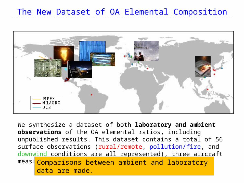
The New Dataset of OA Elemental Composition

MILAGROIMPEX

DC3

We synthesize a dataset of both laboratory and ambient observations of the OA elemental ratios, including unpublished results. This dataset contains a total of 56 surface observations (rural/remote, pollution/fire, and downwind conditions are all represented), three aircraft measurements, and chamber/flow-tube results.Comparisons between ambient and laboratory

data are made.

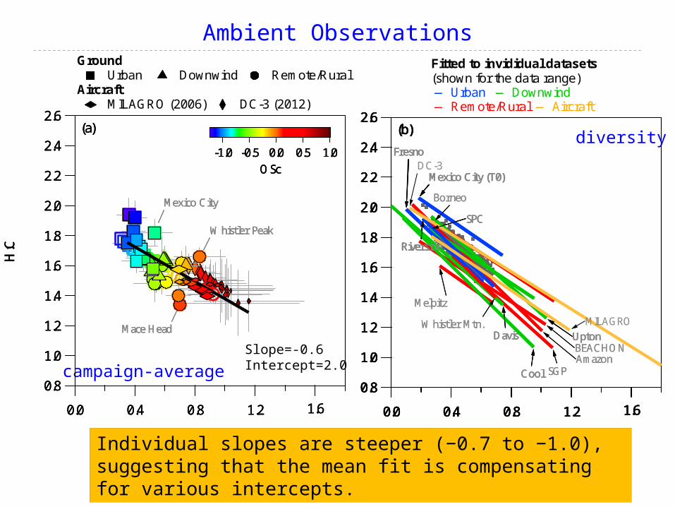
Ambient Observations

2.6

2.4

2.2

2.0

1.8

1.6

1.4

1.2

1.0

0.8

H:C

1.61.20.80.40.0

O:C

-1.0 -0.5 0.0 0.5 1.0OSc

(a)

Mexico City

Whistler Peak

Mace Head

Ground Urban Downwind Remote/Rural

Aircraft MILAGRO (2006) DC-3 (2012)

2.6

2.4

2.2

2.0

1.8

1.6

1.4

1.2

1.0

0.8

H:C

1.61.20.80.40.0

O:C

-1.0 -0.5 0.0 0.5 1.0OSc

(a)

Mexico City

Whistler Peak

Mace Head

campaign-average

2.6

2.4

2.2

2.0

1.8

1.6

1.4

1.2

1.0

0.8

H:C

1.61.20.80.40.0

O:C

-1.0 -0.5 0.0 0.5 1.0OSc

(a)

Mexico City

Whistler Peak

Mace Head

Slope=-0.6Intercept=2.0

2.6

2.4

2.2

2.0

1.8

1.6

1.4

1.2

1.0

0.8

H:C

1.61.20.80.40.0

O:C

(b)

Riverside

2.6

2.4

2.2

2.0

1.8

1.6

1.4

1.2

1.0

0.8

H:C

1.61.20.80.40.0

O:C

(b)

Riverside

Mexico City (T0)

Fresno

2.6

2.4

2.2

2.0

1.8

1.6

1.4

1.2

1.0

0.8

H:C

1.61.20.80.40.0

O:C

(b)

Riverside

Mexico City (T0)

Fresno

Cool

Davis

SPC

Upton

2.6

2.4

2.2

2.0

1.8

1.6

1.4

1.2

1.0

0.8

H:C

1.61.20.80.40.0

O:C

(b)

Riverside

Mexico City (T0)

Fresno

Borneo

AmazonSGP

BEACHON

Melpitz

Cool

Davis

SPC

UptonWhistler Mtn.

2.6

2.4

2.2

2.0

1.8

1.6

1.4

1.2

1.0

0.8

H:C

1.61.20.80.40.0

O:C

(b)

Riverside

Mexico City (T0)

Fresno

Borneo

DC-3

AmazonSGP

BEACHON

Melpitz

Cool

Davis

SPC

UptonMILAGROWhistler Mtn.

Fitted to invididual datasets(shown for the data range) — Urban — Downwind — Remote/Rural — Aircraft

Individual slopes are steeper (−0.7 to −1.0), suggesting that the mean fit is compensating for various intercepts.

diversity

Laboratory Measurements

2.6

2.4

2.2

2.0

1.8

1.6

1.4

1.2

1.0

0.8

H:C

1.61.20.80.40

O:C

n nn nn

n

nnn

ppp

ooooxxx

x

aaaaaaaaaa

aaaaaaaaaaaaaaaaaaaaaaaaaaaaaaaaaaaaaaaaaaaaa

aaaaaaaaaaaaaa

aaaaaaaaa aaaaaaaaa

aaaaaaaaa aaaaaX X

X

X

X

TTT

ZZZ

rrr

r

r

rr

rrrrr

b

bbb

b

b

b

bb

bI

III IIIIIIII

InInInInSSSSSSSS

S

SMMM

MMMM MMLLLLLLL

dg

d

d

d

ttcc

c cccGGG

e

e

e

ee

R

E

(c)

Biomass burning OA (b)Anthropogenic POABiogenic SOA Aromatic SOAFresh IVOC SOAGlyoxal aqueous uptake (G)Marine Emissions (R)IEPOX-OA monoterpene ELVOC


1.61.20.80.40

O:C

Anthropogenic (POA+SVOC/IVOC)

(d)

SOA (gas + particle)

1086420

Biomass burning (POA+SVOC/IVOC) (day)

Heterogeneous Oxidation squalane OA Lubricating oil particles glyoxal OA (aquesous)

2.6

2.4

2.2

2.0

1.8

1.6

1.4

1.2

1.0

0.8

1.61.20.80.40

O:C


(d)


1086420



2.6

2.4

2.2

2.0

1.8

1.6

1.4

1.2

1.0

0.8

1.61.20.80.40

O:C


(d)


1086420



2.6

2.4

2.2

2.0

1.8

1.6

1.4

1.2

1.0

0.8

H:C

1.61.20.80.40

O:C

n nn nn

n

nnn

ppp

ooooxxx

x

aaaaaaaaaa


aaaaaaaaaaaaaa

aaaaaaaaa aaaaaaaaa

aaaaaaaaa aaaaaX X

X

X

X

TTT

ZZZ

rrr

r

r

rr

rrrrr

b

bbb

b

b

b

bb

bI

III IIIIIIII

InInInInSSSSSSSS

S

SMMM

MMMM MMLLLLLLL

dg

d

d

d

ttcc

c cccGGG

e

e

e

ee

R

E

(c) 2.6

2.4

2.2

2.0

1.8

1.6

1.4

1.2

1.0

0.8

1.61.20.80.40

O:C


(d)


1086420



(d) downwind TSOA & Aging(g/p)ISOA(NOx)

ASOA & Aging(g/p)BBOA & Aging(g/p)APOA & Aging(g/p)

(c) Mexico City TSOAISOA(NOx)

ASOABBOA & Aging(g/p)APOA & Aging(g/p)

2.4

2.0

1.6

1.2

0.8

H:C

1.20.80.40.0

(e) Monoterpene-dominant TSOA & Aging(g/p)

Add ELVOCAdd APOA, BBOA & Aging

ManitouWhistlerMountain

2.4

2.0

1.6

1.2

0.8

H:C

(a) Riverside TSOAISOA(NOx)

ASOA

-1.0

-0.5

Add APOA

Lab vs. Field #1: Statistical Mixtures Compared to Ambient

Consistencies

missing sources and pathways which maintain high H:C in areas polluted areas

1.20.80.40.0

(g) Rainforest TSOA & Aging(g/p)ISOA & Aging(g/p)IEPOXp, ELVOC

Amazon

Borneo

Add APOA, Aged BBOAAdd GSOA & Aging

Marine OA

1.61.20.80.40.0

AircraftAmbient

Add GSOA & Aging

TSOA & Aging(g/p)ISOA(NOx)

ASOA & Aging(g/p)BBOA & Aging(g/p)APOA & Aging(g/p)

ELVOC

(h)

Low NOx isoprene chemistry and glyoxal-type of aqueous-phase chemistry can drive the match

lab experiments do not adequately mimic ambient (mixtures? extend of aging?)

Lab vs. Field #2: Observationally-Based Model Simulation

Step 1: SOA yields to reflect recent measurementsStep 2: Account for semi-volatile POA emissionsStep 3: Assign elemental ratios to POA/SOA types simulated in model based on lab dataStep 4: Age gas-phase organics based on flow-tube data but end point constrained by field obs. (50% increase in burden)

Emissions FromFossil Fuel

BiofuelBiomass Burning

VOC

HydrophobicO-POAn

Oxidation Products

SOGi

Gas-phase Particle-phase

*,i iCSOAi

HydrophilicI-POAn

Marine Emissions

Biogenic Emissions

×0.5

1.15d

IsopreneMonoterpenesSesquiterpenes

Aromatics

×0.5

OH, O3

NO3

OH, O3

NO3

kage, jSVOCj SVOC-SOA2, j

SOG-SOA1, i

kcarbon, j×85%

×15%

SVOC-SOA1, j

SOG-SOA2, i kage, ikcarbon, i

Marine POA

End point:O:C=1.1H:C=1.4(defined by field obs)

(GEOS-Chem v9-01-03)

Aging Dramatically Alters Simulation of OA Elemental Composition

Aging leads to

- more pronounced spatial variability (a wider range)

- more pronounced seasonality over continents

Surface distributions

O:C

H:C

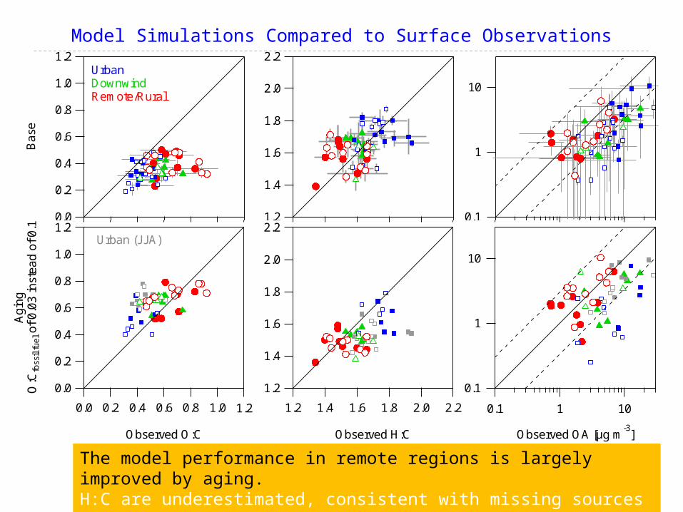
Model Simulations Compared to Surface Observations1.2

1.0

0.8

0.6

0.4

0.2

0.0

Ba

se

1.2

1.0

0.8

0.6

0.4

0.2

0.0

Ag

ing

1.2

1.0

0.8

0.6

0.4

0.2

0.0

Ag

ing

O:C

foss

il fu

el o

f 0.

03

inst

ead

of

0.1

1.21.00.80.60.40.20.0

Observed O:C

2.2

2.0

1.8

1.6

1.4

1.22.2

2.0

1.8

1.6

1.4

1.22.2

2.0

1.8

1.6

1.4

1.2

2.22.01.81.61.41.2

Observed H:C

0.1

1

10

0.1

1

10

0.1

1

10

0.1 1 10

Observed OA [µg m-3

]

UrbanDownwindRemote/Rural

Urban (JJA)

1.2

1.0

0.8

0.6

0.4

0.2

0.0B

ase

1.2

1.0

0.8

0.6

0.4

0.2

0.0

Ag

ing

1.2

1.0

0.8

0.6

0.4

0.2

0.0

Ag

ing

O:C

foss

il fu

el o

f 0.

03

inst

ead

of

0.1

1.21.00.80.60.40.20.0

Observed O:C

2.2

2.0

1.8

1.6

1.4

1.22.2

2.0

1.8

1.6

1.4

1.22.2

2.0

1.8

1.6

1.4

1.2

2.22.01.81.61.41.2

Observed H:C

0.1

1

10

0.1

1

10

0.1

1

10

0.1 1 10

Observed OA [µg m-3

]

UrbanDownwindRemote/Rural

Urban (JJA)

The model performance in remote regions is largely improved by aging.H:C are underestimated, consistent with missing sources or pathways for high H:C.

Heterogeneous oxidation effectively helps to reproduce the vertical gradient.

10

8

6

4

2

0

Alti

tude

(km

)

1.21.00.80.60.4

O:C

Observation Base Aging Aging w/. SOA heterogeneous aging Aging w/. 5xSOG -> SOA Aging w/. 25 KJ/mol enthalpy Aging w/. 2xEpoa

1086420

OA

(b) DC-3

4.03.02.01.00.0

OA

10

8

6

4

2

0

Alti

tude

(km

)

1.21.00.80.60.4

O:C

(a) IMPEX

10

8

6

4

2

0

Alti

tude

(km

)

1.21.00.80.60.4

O:C

Observation Base Aging Aging w/. SOA heterogeneous aging Aging w/. 5xSOG -> SOA Aging w/. 25 KJ/mol enthalpy Aging w/. 2xEpoa

O:C OA1.701.601.501.401.30

H:CH:C

Cannot reproduce variability in observed H:C.

1×10-13 cm3 molecule−1 s−1

Conclusions

The disconnect between laboratory and ambient OA elemental composition, especially for areas influenced by pollution and/or fires -> missing sources and/or pathways which maintain high H:C -> linked to missing OA mass in those regions

Simple, measurement-based aging scheme largely improves simulation of elemental composition. Including heterogeneous oxidation helps reproduce the vertical profile.

2.6

2.4

2.2

2.0

1.8

1.6

1.4

1.2

1.0

0.8

H:C

1.61.20.80.40

O:C

n nn nn

n

nnn

ppp

ooooxxx

x

aaaaaaaaaa


aaaaaaaaaaaaaa

aaaaaaaaa aaaaaaaaa

aaaaaaaaa aaaaaX X

X

X

X

TTT

ZZZ

rrr

r

r

rr

rrrrr

b

bbb

b

b

b

bb

b

dg

d

d

d

ttcc

c cccGGG

R

E


2.6

2.4

2.2

2.0

1.8

1.6

1.4

1.2

1.0

0.8

H:C

1.61.20.80.40

O:C

n nn nn

n

nnn

ppp

ooooxxx

x

aaaaaaaaaa


aaaaaaaaaaaaaa

aaaaaaaaa aaaaaaaaa

aaaaaaaaa aaaaaX X

X

X

X

TTT

ZZZ

rrr

r

r

rr

rrrrr

b

bbb

b

b

b

bb

b

dg

d

d

d

ttcc

c cccGGG

R

E

(c)

+ alcohol/peroxide

+ carboxylic acid

Thank you!

modeling elemental composition of organic aerosol: exploiting laboratory and ambient measurement and...

Documents