Modeling Illiquidity Premia forAlternative Investments

The Swiss CFA Society, Zurich & GenevaRenato Staub, November 6 & 7, 2008

2

Problem

Most alternative investments are illiquid.

This reduces the investor’s flexibility.

In a rational world, this should be compensated.

For asset allocation, we need to know how illiquidity is compensated.

The Capital Asset Pricing Model (CAPM) does not deal with illiquidity.

3

Examinations

How do we define illiquidity?

How does literature define illiquidity?

What does literature say about compensation for illiquidity?

How do we approach illiquidity compensation?

How does our approach fit into our framework for modeling asset returns?

4

Definition

— Finance 101 Class: “Liquidity is the price elasticity with regard to the turnover of the respective security.”

— Gastineau: “Liquidity is a market condition in which enough units […] are traded […] without significant impact on price stability.”

In most instances, “liquidity” is associated with the costliness of a trade, and it is measured in terms of its bid-ask spread.

However, we are concerned about the fact that alternative assets are…

Liquidity: Definition

5

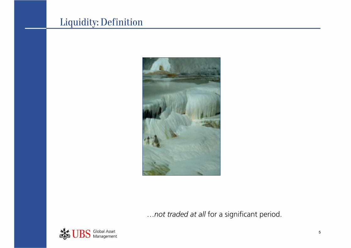
Liquidity: Definition

…not traded at all for a significant period.

6

Literature

Irrelevant literature (for asset mgt.) – trading based (90% of all literature)

— Amihud/Mendelson (1986/1, 1986/2)

— Longstaff (1995, 1999)

Relevant literature – discount based

— Silber (1991) examines restricted stocks (SEC 144) and finds a 34% average discount for a 2-year illiquidity.

— Chaffe (1993) thinks a fair discount for illiquidity equals the value of a put option. The discounts turn out to be very large in some instances.

— Smith/Smith/Williams (2000) think large illiquidity discounts are not justified economically. They claim that studies providing large discounts are flawed.

7

Literature: Judgement

Literature

— Often operates with biased data

— Concentrates on particular selected aspects

— Provides stand-alone investigations

— Is trading based (in 90% of all instances)

— Makes unrealistic assumptions

Probably, most studies overestimate illiquidity compensation .

We have hands-on experience with illiquidity compensation: UBS EIP stocks

— 3-year lock in

— 13% discount (pay 100, get 115)

— UBS saves about a 9% in pension fund contribution— Hence, 4% net discount

— Further, UBS is not forced to issue EIP stocks

8

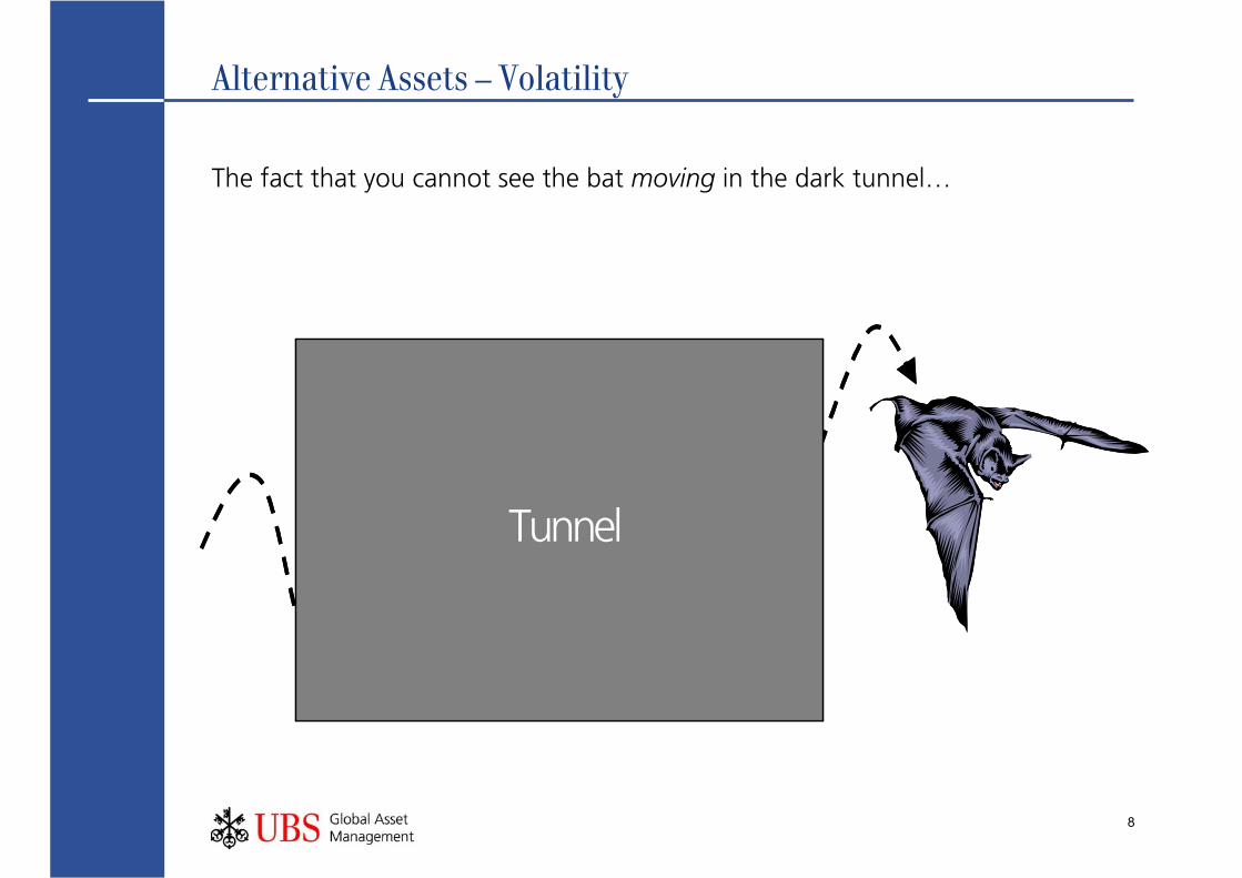
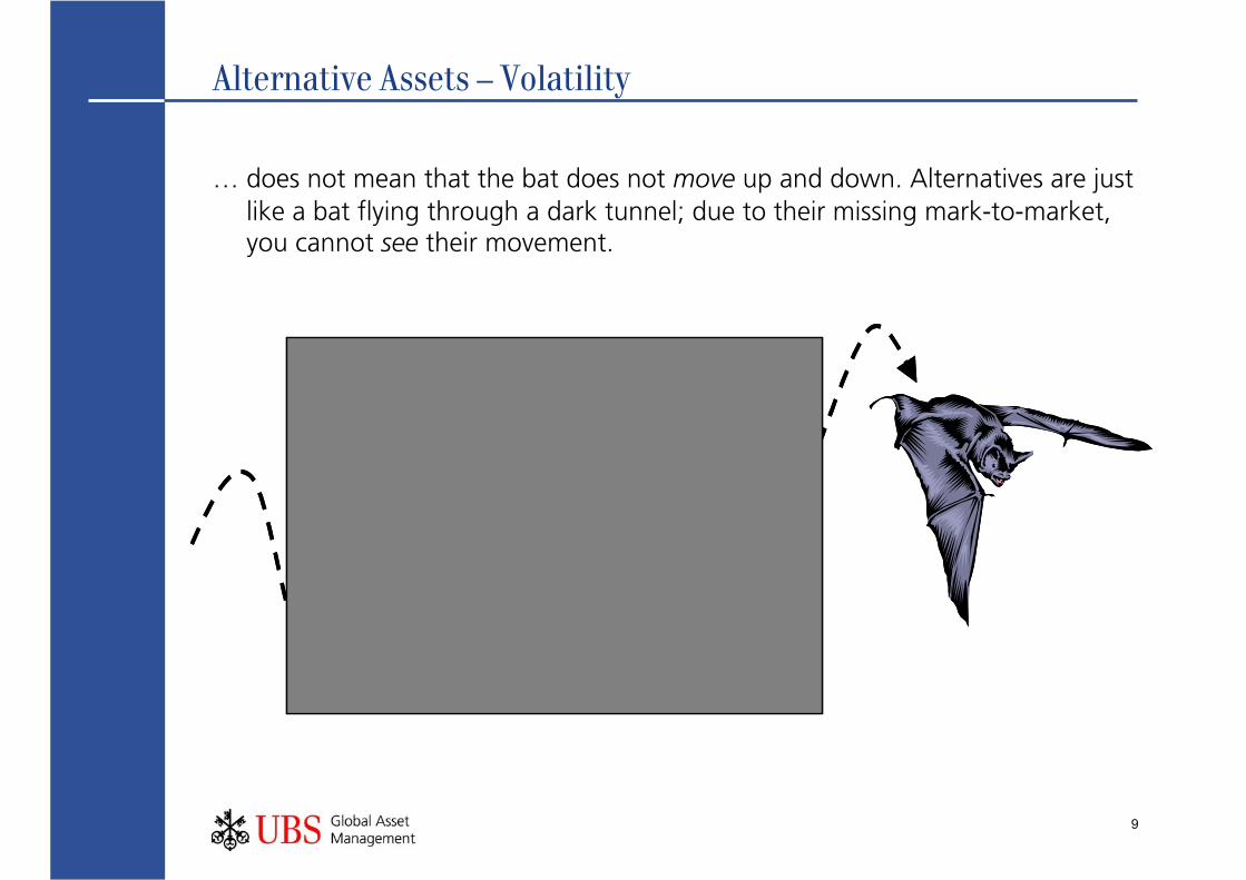
Alternative Assets – Volatility

The fact that you cannot see the bat moving in the dark tunnel…

TunnelTunnel

9

Alternative Assets – Volatility

… does not mean that the bat does not move up and down. Alternatives are just like a bat flying through a dark tunnel; due to their missing mark-to-market, you cannot see their movement.

10

5

10

15

20

25

30

1985 '87 '89 '91 '93 '95 '97 1999

0

5

10

15

20

25

30

35

40

45

50

S&P 500 (lhs)Venture Capital (rhs)

End Year

An

nu

al P

erce

nt

Ret

urn

An

nu

al Percent R

eturn

Alternative Assets – CorrelationInternal Rates of Return for 5-Year Holding Periods

Sources: Venture Economics, Standard & Poor’s

11

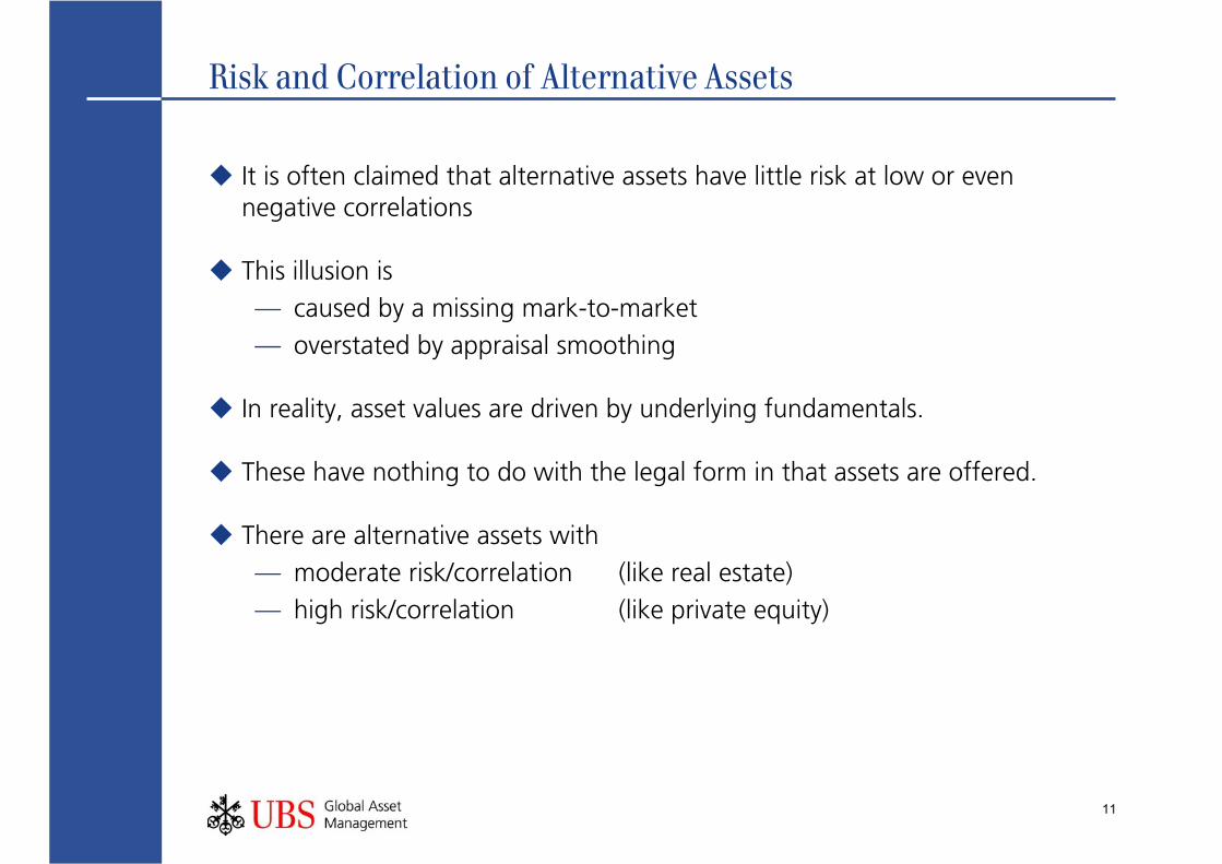
Risk and Correlation of Alternative Assets

It is often claimed that alternative assets have little risk at low or even negative correlations

This illusion is

— caused by a missing mark-to-market

— overstated by appraisal smoothing

In reality, asset values are driven by underlying fundamentals.

These have nothing to do with the legal form in that assets are offered.

There are alternative assets with

— moderate risk/correlation (like real estate)

— high risk/correlation (like private equity)

12

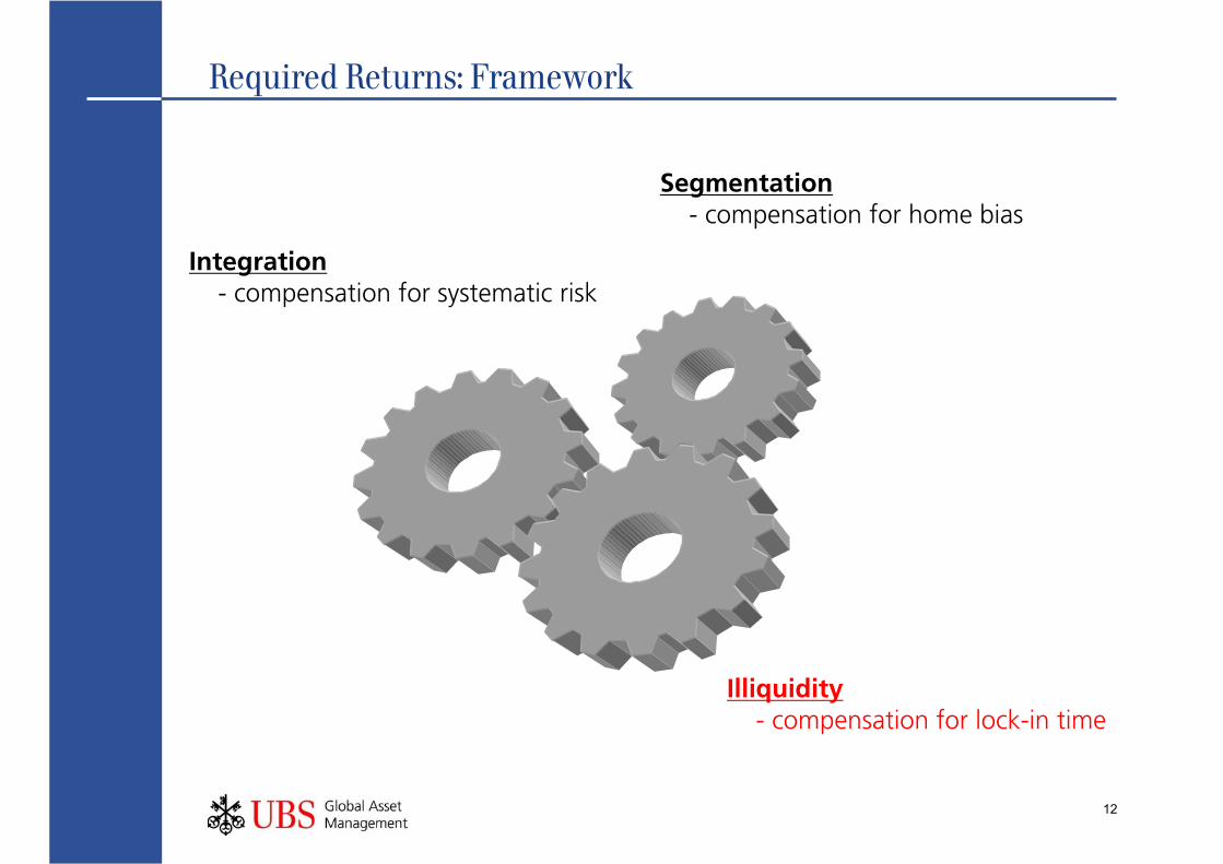
Required Returns: Framework

Integration- compensation for systematic risk

Segmentation- compensation for home bias

Illiquidity- compensation for lock-in time

13

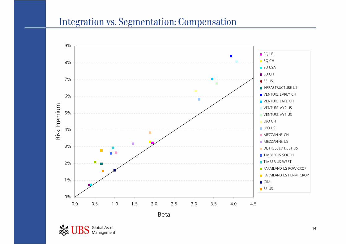
Integration vs. Segmentation

Integration means a world of no market imperfection.

The risk premia are based on a CAPM-like, single factor.

Greatest challenge in practice: defining “the market”.

Segmentation depicts a world without free capital flows between markets.

In a segmented world, the marginal investor is a local investor.

In a segmented world, an asset is compensated according to its total rather than its systematic risk.

In reality, a market is neither fully integrated nor absolutely segmented.

Its risk premium is estimated based on a weighted mean between integration and segmentation.

14

Integration vs. Segmentation: Compensation

0%

1%

2%

3%

4%

5%

6%

7%

8%

9%

0.0 0.5 1.0 1.5 2.0 2.5 3.0 3.5 4.0 4.5

Beta

Ris

k Pr

emiu

mEQ US

EQ CH

BD USA

BD CH

RE US

INFRASTRUCTURE US

VENTURE EARLY CH

VENTURE LATE CH

VENTURE VY2 US

VENTURE VY7 US

LBO CH

LBO US

MEZZANINE CH

MEZZANINE US

DISTRESSED DEBT US

TIMBER US SOUTH

TIMBER US WEST

FARMLAND US ROW CROP

FARMLAND US PERM. CROP

GIM

RE US

15

Illiquidity Compensation: Approaches

Jaffe’s put option approach

Our Sharpe ratio approach

Our put option approach

16

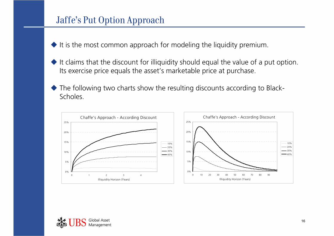
Jaffe’s Put Option Approach

It is the most common approach for modeling the liquidity premium.

It claims that the discount for illiquidity should equal the value of a put option. Its exercise price equals the asset’s marketable price at purchase.

The following two charts show the resulting discounts according to Black-Scholes.

Chaffe's Approach - According Discount

0%

5%

10%

15%

20%

25%

0 1 2 3 4

Illiquidity Horizon (Years)

10%

20%

30%

40%

Chaffe's Approach - According Discount

0%

5%

10%

15%

20%

25%

0 10 20 30 40 50 60 70 80 90

Illiquidity Horizon (Years)

10%

20%

30%

40%

17

Jaffe’s Approach seems too generous

The discount increases with a rising illiquidity horizon, turns at some point and approaches zero asymptotically.

In the short run, this means free shortfall insurance combined with unlimited upward potential. It litterally implies no real risk-return trade-off.

For longer horizons, the implied illiquidity premium decreases with an increasing illiquidity horizon, whereas practical evidence implies the contrary.

Full shortfall insurance is fairly arbitrary from a statistical perspective, as there is no inherent relationship with both the asset’s risk and the length of the lock-in.

18

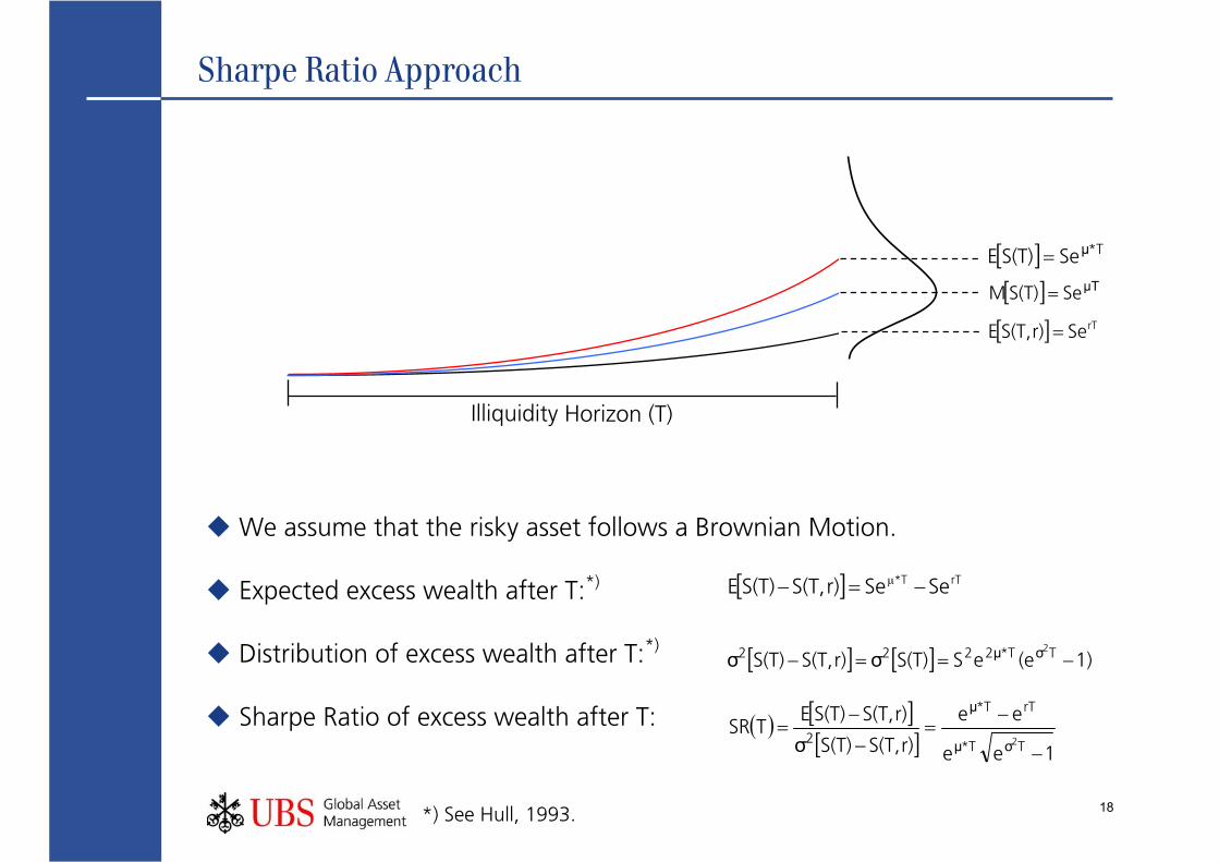
Sharpe Ratio Approach

We assume that the risky asset follows a Brownian Motion.

Expected excess wealth after T:*)

Distribution of excess wealth after T:*)

Sharpe Ratio of excess wealth after T:

Illiquidity Horizon (T)

[ ] T*μSeS(T)E =

[ ] μTSeS(T)M =

[ ] rTSer)S(T,E =

[ ] rTT* SeSer)S(T,S(T)E −=− μ

[ ] [ ] 1)(eeSS(T)σr)S(T,S(T)σ TσT*2μ222 2

−==−

( ) [ ][ ] 1ee

ee

r)S(T,S(T)σr)S(T,S(T)E

TSRTσT*μ

rTT*μ

2 2

−

−=

−

−=

*) See Hull, 1993.

19

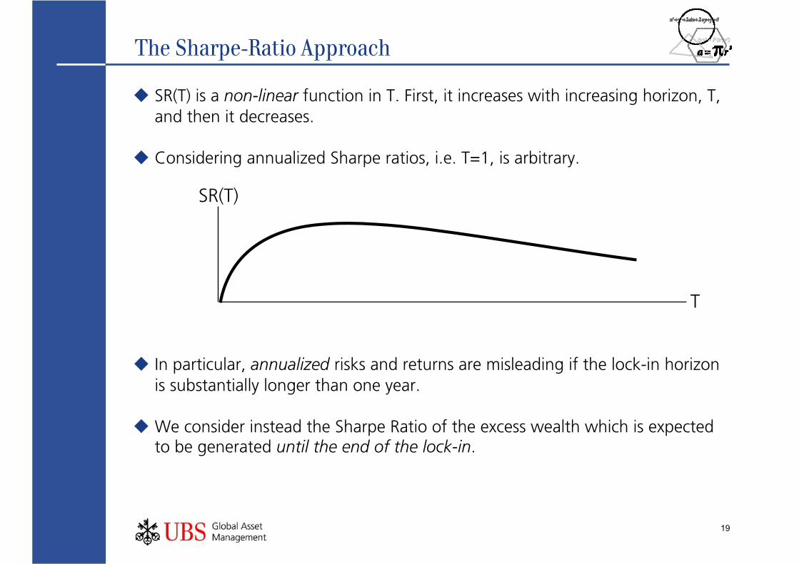
The Sharpe-Ratio Approach

SR(T) is a non-linear function in T. First, it increases with increasing horizon, T, and then it decreases.

Considering annualized Sharpe ratios, i.e. T=1, is arbitrary.

In particular, annualized risks and returns are misleading if the lock-in horizon is substantially longer than one year.

We consider instead the Sharpe Ratio of the excess wealth which is expected to be generated until the end of the lock-in.

T

SR(T)

20

Our Sharpe Ratio Approach - Example

Assume

μ=10% (continuous return of asset, fully reinvested)

σ=20% (risk of asset)

r=5% (riskless return, fully reinvested)

SR = (10-5) / 20 = 0.25 (excess return / distrib. of excess return)

After a time horizon, T, of 5 years for instance, we get

V=182% (expected value of asset)

Σ=60% (distribution of asset’s value)

W=128% (expected value of riskless asset)

SR(T) = (182-128) / 60 = 0.90 (excess value / distrib. of excess value)

SR(T) is the excess value divided by its distribution, rather than the annualized excess return divided by its distribution.

21

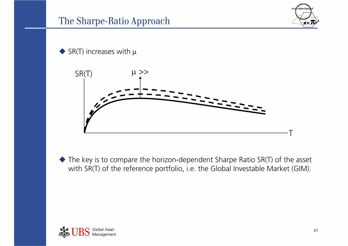
The Sharpe-Ratio Approach

SR(T) increases with μ

The key is to compare the horizon-dependent Sharpe Ratio SR(T) of the asset with SR(T) of the reference portfolio, i.e. the Global Investable Market (GIM).

T

SR(T) μ >>

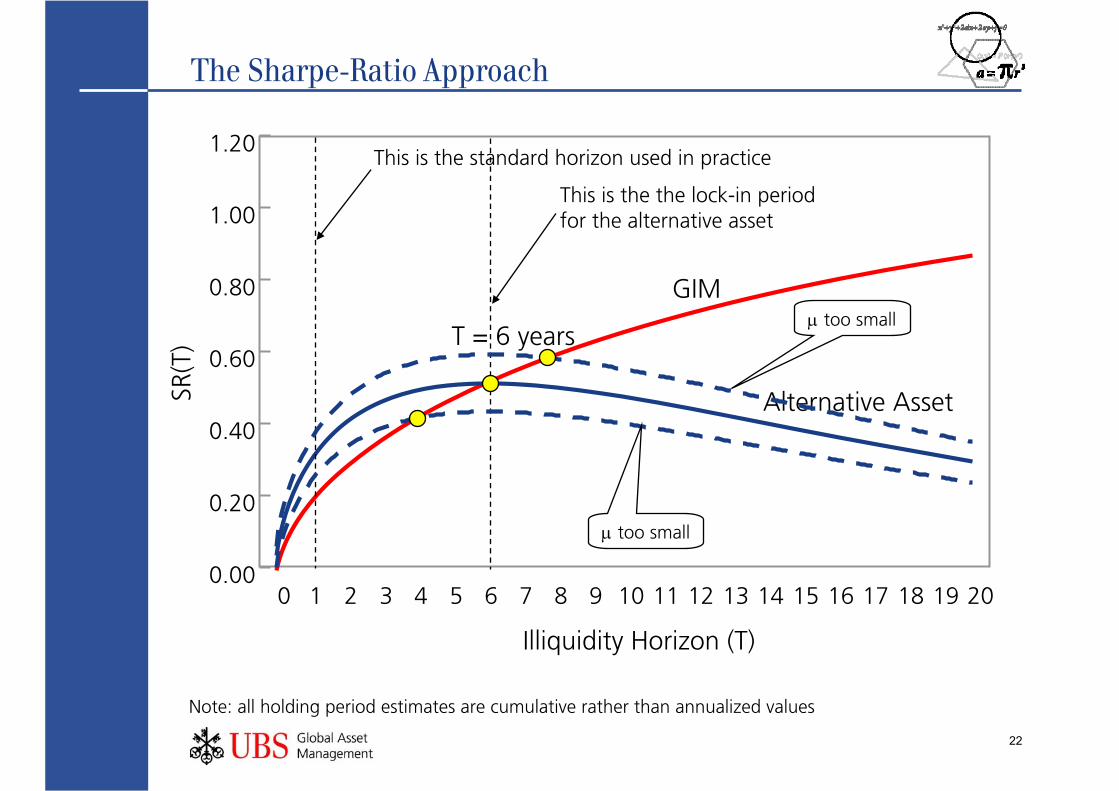
22

0 1 2 3 4 5 6 7 8 9 10 11 12 13 14 15 16 17 18 19 200.00

0.20

0.40

0.60

0.80

1.00

1.20

Illiquidity Horizon (T)

SR(T

)

The Sharpe-Ratio Approach

GIM

T = 6 years

Alternative Asset

Note: all holding period estimates are cumulative rather than annualized values

This is the standard horizon used in practice

This is the the lock-in periodfor the alternative asset

μ too small

μ too small

23

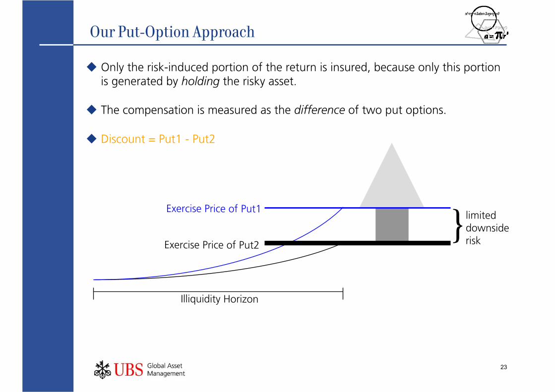
Our Put-Option Approach

Only the risk-induced portion of the return is insured, because only this portion is generated by holding the risky asset.

The compensation is measured as the difference of two put options.

Discount = Put1 - Put2

Illiquidity Horizon

Exercise Price of Put1

Exercise Price of Put2} limited

downsiderisk

24

Integration into our Existing Framework

Calculate illiquidity compensation with total risk of the alternative asset as an input: full integration.

Calculate illiquidity compensation with the systematic risk of the alternative asset as an input: full segmentation.

Define the weighting scheme for integration / segmentation of alternative assets.

Total premia (risk premia plus liquidity premia) is the weighted mean.

25

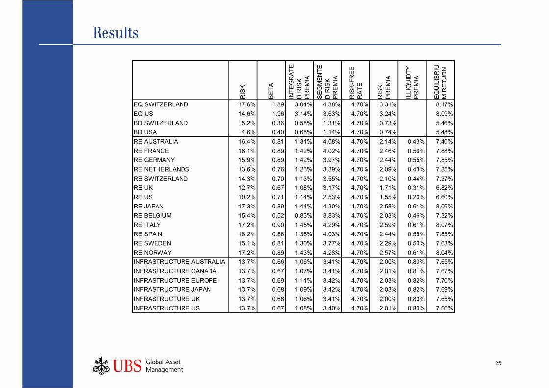
Results

RIS

K

BE

TA

INTE

GR

ATE

D R

ISK

P

RE

MIA

SE

GM

EN

TED

RIS

K

PR

EM

IA

RIS

K-F

RE

E

RA

TE

RIS

K

PR

EM

IA

ILLI

QU

IDTY

P

RE

MIA

EQ

UIL

IBR

IUM

RE

TUR

N

EQ SWITZERLAND 17.6% 1.89 3.04% 4.38% 4.70% 3.31% 8.17%EQ US 14.6% 1.96 3.14% 3.63% 4.70% 3.24% 8.09%BD SWITZERLAND 5.2% 0.36 0.58% 1.31% 4.70% 0.73% 5.46%BD USA 4.6% 0.40 0.65% 1.14% 4.70% 0.74% 5.48%RE AUSTRALIA 16.4% 0.81 1.31% 4.08% 4.70% 2.14% 0.43% 7.40%RE FRANCE 16.1% 0.89 1.42% 4.02% 4.70% 2.46% 0.56% 7.88%RE GERMANY 15.9% 0.89 1.42% 3.97% 4.70% 2.44% 0.55% 7.85%RE NETHERLANDS 13.6% 0.76 1.23% 3.39% 4.70% 2.09% 0.43% 7.35%RE SWITZERLAND 14.3% 0.70 1.13% 3.55% 4.70% 2.10% 0.44% 7.37%RE UK 12.7% 0.67 1.08% 3.17% 4.70% 1.71% 0.31% 6.82%RE US 10.2% 0.71 1.14% 2.53% 4.70% 1.55% 0.26% 6.60%RE JAPAN 17.3% 0.89 1.44% 4.30% 4.70% 2.58% 0.61% 8.06%RE BELGIUM 15.4% 0.52 0.83% 3.83% 4.70% 2.03% 0.46% 7.32%RE ITALY 17.2% 0.90 1.45% 4.29% 4.70% 2.59% 0.61% 8.07%RE SPAIN 16.2% 0.86 1.38% 4.03% 4.70% 2.44% 0.55% 7.85%RE SWEDEN 15.1% 0.81 1.30% 3.77% 4.70% 2.29% 0.50% 7.63%RE NORWAY 17.2% 0.89 1.43% 4.28% 4.70% 2.57% 0.61% 8.04%INFRASTRUCTURE AUSTRALIA 13.7% 0.66 1.06% 3.41% 4.70% 2.00% 0.80% 7.65%INFRASTRUCTURE CANADA 13.7% 0.67 1.07% 3.41% 4.70% 2.01% 0.81% 7.67%INFRASTRUCTURE EUROPE 13.7% 0.69 1.11% 3.42% 4.70% 2.03% 0.82% 7.70%INFRASTRUCTURE JAPAN 13.7% 0.68 1.09% 3.42% 4.70% 2.03% 0.82% 7.69%INFRASTRUCTURE UK 13.7% 0.66 1.06% 3.41% 4.70% 2.00% 0.80% 7.65%INFRASTRUCTURE US 13.7% 0.67 1.08% 3.40% 4.70% 2.01% 0.80% 7.66%

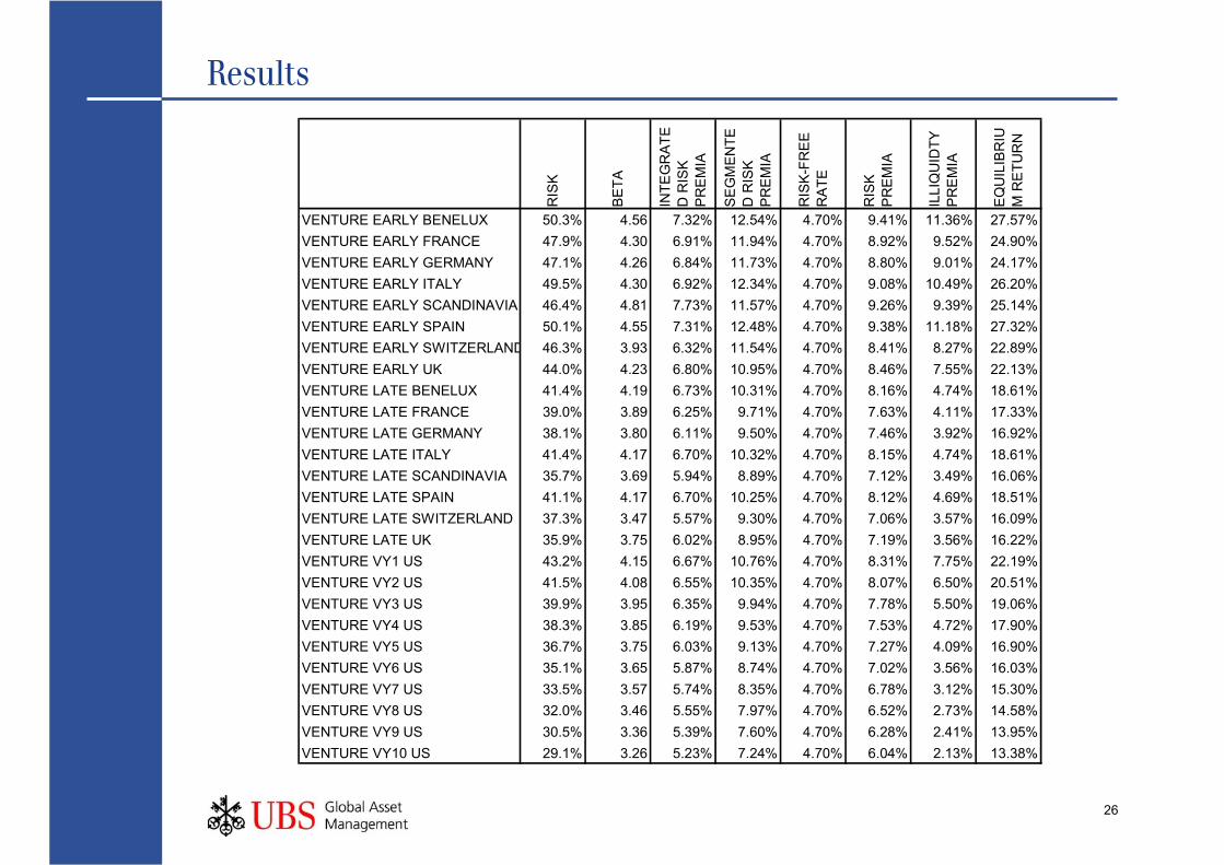
26

Results

RIS

K

BE

TA

INTE

GR

ATE

D R

ISK

P

RE

MIA

SE

GM

EN

TED

RIS

K

PR

EM

IA

RIS

K-F

RE

E

RA

TE

RIS

K

PR

EM

IA

ILLI

QU

IDTY

P

RE

MIA

EQ

UIL

IBR

IUM

RE

TUR

N

VENTURE EARLY BENELUX 50.3% 4.56 7.32% 12.54% 4.70% 9.41% 11.36% 27.57%VENTURE EARLY FRANCE 47.9% 4.30 6.91% 11.94% 4.70% 8.92% 9.52% 24.90%VENTURE EARLY GERMANY 47.1% 4.26 6.84% 11.73% 4.70% 8.80% 9.01% 24.17%VENTURE EARLY ITALY 49.5% 4.30 6.92% 12.34% 4.70% 9.08% 10.49% 26.20%VENTURE EARLY SCANDINAVIA 46.4% 4.81 7.73% 11.57% 4.70% 9.26% 9.39% 25.14%VENTURE EARLY SPAIN 50.1% 4.55 7.31% 12.48% 4.70% 9.38% 11.18% 27.32%VENTURE EARLY SWITZERLAND 46.3% 3.93 6.32% 11.54% 4.70% 8.41% 8.27% 22.89%VENTURE EARLY UK 44.0% 4.23 6.80% 10.95% 4.70% 8.46% 7.55% 22.13%VENTURE LATE BENELUX 41.4% 4.19 6.73% 10.31% 4.70% 8.16% 4.74% 18.61%VENTURE LATE FRANCE 39.0% 3.89 6.25% 9.71% 4.70% 7.63% 4.11% 17.33%VENTURE LATE GERMANY 38.1% 3.80 6.11% 9.50% 4.70% 7.46% 3.92% 16.92%VENTURE LATE ITALY 41.4% 4.17 6.70% 10.32% 4.70% 8.15% 4.74% 18.61%VENTURE LATE SCANDINAVIA 35.7% 3.69 5.94% 8.89% 4.70% 7.12% 3.49% 16.06%VENTURE LATE SPAIN 41.1% 4.17 6.70% 10.25% 4.70% 8.12% 4.69% 18.51%VENTURE LATE SWITZERLAND 37.3% 3.47 5.57% 9.30% 4.70% 7.06% 3.57% 16.09%VENTURE LATE UK 35.9% 3.75 6.02% 8.95% 4.70% 7.19% 3.56% 16.22%VENTURE VY1 US 43.2% 4.15 6.67% 10.76% 4.70% 8.31% 7.75% 22.19%VENTURE VY2 US 41.5% 4.08 6.55% 10.35% 4.70% 8.07% 6.50% 20.51%VENTURE VY3 US 39.9% 3.95 6.35% 9.94% 4.70% 7.78% 5.50% 19.06%VENTURE VY4 US 38.3% 3.85 6.19% 9.53% 4.70% 7.53% 4.72% 17.90%VENTURE VY5 US 36.7% 3.75 6.03% 9.13% 4.70% 7.27% 4.09% 16.90%VENTURE VY6 US 35.1% 3.65 5.87% 8.74% 4.70% 7.02% 3.56% 16.03%VENTURE VY7 US 33.5% 3.57 5.74% 8.35% 4.70% 6.78% 3.12% 15.30%VENTURE VY8 US 32.0% 3.46 5.55% 7.97% 4.70% 6.52% 2.73% 14.58%VENTURE VY9 US 30.5% 3.36 5.39% 7.60% 4.70% 6.28% 2.41% 13.95%VENTURE VY10 US 29.1% 3.26 5.23% 7.24% 4.70% 6.04% 2.13% 13.38%

27

Results

RIS

K

BE

TA

INTE

GR

ATE

D R

ISK

P

RE

MIA

SE

GM

EN

TED

RIS

K

PR

EM

IA

RIS

K-F

RE

E

RA

TE

RIS

K

PR

EM

IA

ILLI

QU

IDTY

P

RE

MIA

EQ

UIL

IBR

IUM

RE

TUR

N

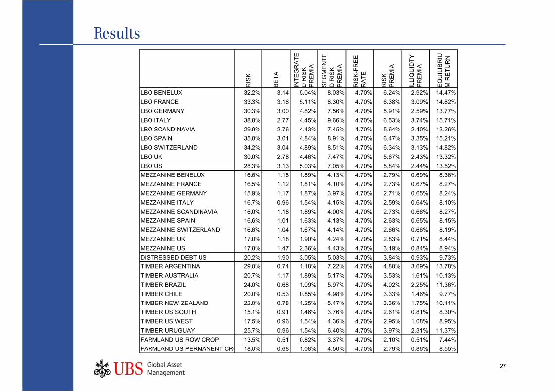
LBO BENELUX 32.2% 3.14 5.04% 8.03% 4.70% 6.24% 2.92% 14.47%LBO FRANCE 33.3% 3.18 5.11% 8.30% 4.70% 6.38% 3.09% 14.82%LBO GERMANY 30.3% 3.00 4.82% 7.56% 4.70% 5.91% 2.59% 13.77%LBO ITALY 38.8% 2.77 4.45% 9.66% 4.70% 6.53% 3.74% 15.71%LBO SCANDINAVIA 29.9% 2.76 4.43% 7.45% 4.70% 5.64% 2.40% 13.26%LBO SPAIN 35.8% 3.01 4.84% 8.91% 4.70% 6.47% 3.35% 15.21%LBO SWITZERLAND 34.2% 3.04 4.89% 8.51% 4.70% 6.34% 3.13% 14.82%LBO UK 30.0% 2.78 4.46% 7.47% 4.70% 5.67% 2.43% 13.32%LBO US 28.3% 3.13 5.03% 7.05% 4.70% 5.84% 2.44% 13.52%MEZZANINE BENELUX 16.6% 1.18 1.89% 4.13% 4.70% 2.79% 0.69% 8.36%MEZZANINE FRANCE 16.5% 1.12 1.81% 4.10% 4.70% 2.73% 0.67% 8.27%MEZZANINE GERMANY 15.9% 1.17 1.87% 3.97% 4.70% 2.71% 0.65% 8.24%MEZZANINE ITALY 16.7% 0.96 1.54% 4.15% 4.70% 2.59% 0.64% 8.10%MEZZANINE SCANDINAVIA 16.0% 1.18 1.89% 4.00% 4.70% 2.73% 0.66% 8.27%MEZZANINE SPAIN 16.6% 1.01 1.63% 4.13% 4.70% 2.63% 0.65% 8.15%MEZZANINE SWITZERLAND 16.6% 1.04 1.67% 4.14% 4.70% 2.66% 0.66% 8.19%MEZZANINE UK 17.0% 1.18 1.90% 4.24% 4.70% 2.83% 0.71% 8.44%MEZZANINE US 17.8% 1.47 2.36% 4.43% 4.70% 3.19% 0.84% 8.94%DISTRESSED DEBT US 20.2% 1.90 3.05% 5.03% 4.70% 3.84% 0.93% 9.73%TIMBER ARGENTINA 29.0% 0.74 1.18% 7.22% 4.70% 4.80% 3.69% 13.78%TIMBER AUSTRALIA 20.7% 1.17 1.89% 5.17% 4.70% 3.53% 1.61% 10.13%TIMBER BRAZIL 24.0% 0.68 1.09% 5.97% 4.70% 4.02% 2.25% 11.36%TIMBER CHILE 20.0% 0.53 0.85% 4.98% 4.70% 3.33% 1.46% 9.77%TIMBER NEW ZEALAND 22.0% 0.78 1.25% 5.47% 4.70% 3.36% 1.75% 10.11%TIMBER US SOUTH 15.1% 0.91 1.46% 3.76% 4.70% 2.61% 0.81% 8.30%TIMBER US WEST 17.5% 0.96 1.54% 4.36% 4.70% 2.95% 1.08% 8.95%TIMBER URUGUAY 25.7% 0.96 1.54% 6.40% 4.70% 3.97% 2.31% 11.37%FARMLAND US ROW CROP 13.5% 0.51 0.82% 3.37% 4.70% 2.10% 0.51% 7.44%FARMLAND US PERMANENT CRO 18.0% 0.68 1.08% 4.50% 4.70% 2.79% 0.86% 8.55%

28

Conclusions

Illiquidity premia are a compensation for locking in investments.

Investors who are able to wait should expect to be rewarded for assuming illiquidity.

Mathematical modeling is necessary to derive appropriate illiquidity premia.

Illiquidity premia are an integral part of an investment’s equilibrium return and are an essential factor in deriving asset allocation policy.

The illiquidity premium is not a free lunch – the higher expected return is compensation for the cost of reduced investment flexibility.

The premium for illiquidity is larger when:

— The length of the lock-in period is greater

(less flexibility)

— The riskiness of the investment is higher

(greater uncertainty)

29

Thank you very much for your attention.

Thank you very much for your attention

30

ReferencesAitchison, J., and J.A.C. Brown, 1966, The Lognormal Distribution. Cambridge University Press.

Amihud, Y., and H. Mendelson, 1986, Liquidity and Stock Returns. Financial Analyst’s Journal. May-June, 43-48.

Amihud, Y., and H. Mendelson, 1986, Asset Pricing and the Bid-Ask Spread. Journal of Financial Economics 17, 223-249.

Brinson, Gary P., Jeffry J. Diermeier, and Gary G. Schlarbaum, 1986. A Composite Portfolio Benchmark for Pension Plans. Financial Analysts Journal, March/April, 15-24.

Chaffe, David B.H., 1993, Option Pricing as a Proxy for Discount for Lack of Marketability in Private Company Valuations. Business Valuation Review. December 1993, 182-188.

Hodges, Charles W., Walton R.L. Taylor, and James A. Yoder, 1997. Stocks, Bonds, the Sharpe Ratio, and the Investment Horizon. Financial Analysts Journal, November/December, 74-80.

Hull, Jon C., 1993, Options, Futures, and other Derivatives, Second Edition. Prentice Hall, Englewood Cliffs, NJ.

Longstaff, Francis A., 1999, Optimal Portfolio Choice and the Valuation of Illiquid Securities. Working Paper.

Longstaff, Francis A., 1996, Placing No-Arbitrage Bounds on the Value of Nonmarketable and Thinly-Traded Securities. Advances in Futures and Options Research 8.

Longstaff, Francis A., 1995, How much Can Marketability Affect Security Values?, The Journal of Finance, Vol. L, No. 5.

Mercer Capital, 1998, Why Not Black-Scholes Rather than the Quantitative Marketability Discount Model? Internet-memo (www.bizval.com).

Perold, Andre F., and William F. Sharpe, 1988. Dynamic Strategies for Asset Allocation. Financial Analysts Journal. January-February, 16-27.

Silber, W.L., 1991. Discounts on Restricted Stock: The Impact of Illiquidity on Stock Prices, Financial Analysts Journal, July/August, 60-64.

Singer, Brian and Kevin Terhaar, 1997. Economic Foundations of Capital Market Returns. The Research Foundation of the Institute of Chartered Financial Analysis.

Smith, Janet Kiholm, Richard L. Smith, and Karyn Williams, 2000. The SEC’s “Fair Value” Standard for Mutual Fund Investment in Restricted Shares and Other Illiquid Securities, Working Paper.

Terhaar, Kevin, Renato Staub, and Brian Singer, (2003). The Appropriate Policy Allocation for Alternative Investments. Journal of Portfolio Mangement, Vol. 29, No. 3, 2003.

The New York Times, Thursday, May 10, 2001. A Lifeline, With Conditions, C1 and C7.

Wilmott, Paul, Sam Howison, and Jeff Dewynne, 1995, The Mathematics of Financial Derivatives. Cambridge University Press, Cambridge, UK.

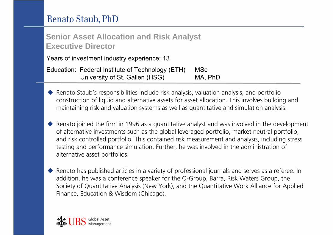
Renato Staub, PhD

Senior Asset Allocation and Risk AnalystExecutive Director

Renato Staub’s responsibilities include risk analysis, valuation analysis, and portfolio construction of liquid and alternative assets for asset allocation. This involves building and maintaining risk and valuation systems as well as quantitative and simulation analysis.

Renato joined the firm in 1996 as a quantitative analyst and was involved in the development of alternative investments such as the global leveraged portfolio, market neutral portfolio, and risk controlled portfolio. This contained risk measurement and analysis, including stress testing and performance simulation. Further, he was involved in the administration of alternative asset portfolios.

Renato has published articles in a variety of professional journals and serves as a referee. Inaddition, he was a conference speaker for the Q-Group, Barra, Risk Waters Group, the Society of Quantitative Analysis (New York), and the Quantitative Work Alliance for Applied Finance, Education & Wisdom (Chicago).

Years of investment industry experience: 13

Education: Federal Institute of Technology (ETH) MScUniversity of St. Gallen (HSG) MA, PhD

32

Publications

[1] Akers, Kurt, and Renato Staub. “Regional Investment Allocations in a Global Timber Market”. Journal of Alternative Investments, Vol. 5, No. 4, 2003.

[2] Calverley, John P., Alan A. Meder, Brian D. Singer, and Renato Staub. “Capital Market Expectations”. Managing Investement Portfolios, CFA Institure, 3rd series, 2007.

[3] Meder, Aaron, and Renato Staub. “Linking Pension Liabilities to Assets”. Society of Actuaries, 2007.

[4] Brian Singer, Renato Staub, and Kevin Terhaar. “Appropriate Policy Allocation for Alternative Investments.” AMIR Conference Proceedings, 2001.

[5] Staub, Renato, and Jerrey Diermeier. “Illiquidity, Segmentation and Returns”. Journal of Investment Management, Vol. 1, No. 1, 2003.

[6] Staub, Renato. “Capital Market Assumptions”. UBS Global Asset Management, Working Paper, 2005.

[7] Staub, Renato. “Multilayer Modeling of a Covariance Matrix.” Journal of Portfolio Management, Vol. 31, No. 3, 2006.

[8] Staub, Renato. “Asset Allocation vs. Security Selection – Baseball with Pitchers only?” Journal of Investing, Vol. 15, No. 3, 2006.

[9] Staub, Renato. “Unlocking the Cage”. Journal of Wealth Management, Vol. 8, No. 5, 2006.

[10] Staub, Renato. “Deploying Alpha Potential”. UBS Global Asset Management, Working Paper, 2006.

[11] Staub, Renato. “Are you about to Handcuff your Information Ratio?”Journal of Asset Management, Vol. 7, No. 5, 2007.

[12] Staub, Renato. “Deploying Alpha: A Strategy to Capture and Leverage the Best Investment Ideas”. A Guide to 130/30 Strategies, Institutional Investor, Summer 2008.

33

Publications

[13] Staub, Renato. “Signal Translation and Portfolio Construction”. UBS Global Asset Management, Working Paper, 2008.

[14] Terhaar Kevin, Renato Staub, and Brian Singer. “Appropriate Policy Allocation for Alternative Investments.”Journal of Portfolio Management, Vol. 29, No. 3, 2003.

[15] Staub, Renato. “Integration of Alternative Investments into the Market Covariance Matrix.” Working Paper, UBS Global Asset Management, 2001.

[16] Staub, Renato. “The Correlation between U.S. Equity and U.S. Bonds.” UBS Global Asset Management, Working Paper, March 2002.

[17] Staub, Renato. “Quarterly Focus: Capital Market Assumptions.” UBS Global Asset Management, Quarterly Investment Strategy, March 31, 2004, p. 4-7.