modeling land surface processes and heavy rainfall in

Modeling Land Surface Processes and Heavy Rainfall in UrbanEnvironments: Sensitivity to Urban Surface Representations

DAN LI, ELIE BOU-ZEID, AND MARY LYNN BAECK

Department of Civil and Environmental Engineering, Princeton University, Princeton, New Jersey

STEPHEN JESSUP

Department of Civil and Environmental Engineering, Princeton University, Princeton, New Jersey,

and Department of Earth and Atmospheric Sciences, Cornell University, Ithaca, New York

JAMES A. SMITH

Department of Civil and Environmental Engineering, Princeton University, Princeton, New Jersey

(Manuscript received 25 October 2012, in final form 8 January 2013)

ABSTRACT

High-resolution simulations with the Weather Research and Forecasting Model (WRF) are used in

conjunction with observational analyses to investigate land surface processes and heavy rainfall over the

Baltimore–Washington metropolitan area. Analyses focus on a 6-day period, 21–26 July 2008, which in-

cludes a major convective rain event (23–24 July), a prestorm period (21–22 July), and a dry-down period

(25–26 July). The performance of WRF in capturing land–atmosphere interactions, the bulk structure of the

atmospheric boundary layer, and the rainfall pattern in urban environments is explored. Results indicate that

WRF captures the incoming radiative fluxes and surfacemeteorological conditions.Mean profiles of potential

temperature and humidity in the atmosphere are also relatively well reproduced, both preceding and fol-

lowing the heavy rainfall period. However, wind features in the lower atmosphere, including low-level jets,

are not accurately reproduced byWRF. The biases in the wind fields play a central role in determining errors

in WRF-simulated rainfall fields. The study also investigates the sensitivity of WRF simulations to different

urban surface representations. It is found that urban surface representations have a significant impact on the

surface energy balance and the rainfall distribution. As the impervious fraction increases, the sensible heat

flux and the ground heat flux increase, while the latent heat flux decreases. The impact of urban surface

representations on precipitation is as significant as that of microphysical parameterizations. The fact that

changing urban surface representations can significantly alter the rainfall field suggests that urbanization plays

an important role in modifying the regional precipitation pattern.

1. Introduction

Precipitation is the primary driver of land surface

hydrological processes and the main component of the

terrestrial water budget (Brutsaert 2005). It also affects

the surface energy budget and land–atmosphere in-

teractions by modifying soil moisture (Betts et al. 1996).

High-resolution modeling of land surface hydrological

processes enabled by the ever-increasing computing

power requires detailed rainfall estimates as inputs

(Wood et al. 2011). However, physically based rain-

fall modeling remains a significant challenge, particu-

larly because of the strong and complex interactions

between synoptic forcing, microphysical processes, land–

atmosphere exchanges, and the evolution of the atmo-

spheric boundary layer (Pielke 2001; Shephard 2005;

Trier et al. 2011; Yeung et al. 2011).

The impact of land–atmosphere exchanges and at-

mospheric boundary layer processes on warm season

rainfall is the subject of active research (Trier et al. 2004,

2008, 2011), including a number of studies with a specific

focus on urban environments (Shephard 2005; Ntelekos

et al. 2007, 2008; Miao et al. 2011; Niyogi et al. 2011;

Corresponding author address:Dan Li, Department of Civil and

Environmental Engineering, Princeton University, 59 Olden St.,

Princeton, NJ 08544.

E-mail: [email protected]

1098 JOURNAL OF HYDROMETEOROLOGY VOLUME 14

DOI: 10.1175/JHM-D-12-0154.1

� 2013 American Meteorological Society

Yeung et al. 2011). In this study, theWeather Research

and Forecasting Model (WRF) is used to investigate

the interactions between land–atmosphere exchanges,

boundary layer processes, and heavy rainfall in the

Baltimore–Washington metropolitan region, where

heavy rainfall is often observed to be associated with

organized thunderstorm systems and induces heavy

flooding (Ntelekos et al. 2007, 2008; Zhang et al.

2009).

WRF is a community model and has multiple pa-

rameterization schemes for each of its five physical

packages: cumulus clouds, microphysics, radiation, plan-

etary boundary layer (PBL), and the surface (Skamarock

and Klemp 2008). Studies have demonstrated that some

of the physics schemes can significantly affect rainfall

modeling. For example, Jankov et al. (2005) analyzed the

sensitivity of warm-season mesoscale convective system

rainfall to different physical parameterizations and con-

cluded that the microphysics and the PBL schemes have

relatively larger impacts than the cumulus schemes. Trier

et al. (2004, 2008, 2011) investigated the impact of land

surface processes, including surface energy partitioning

and changes in soil conditions, on convection initiation

and warm-season precipitation. In this study, we pri-

marily explore the sensitivity of heavy rainfall in WRF

to different urban surface representations by developing

a better understanding of the linkages between land–

atmosphere exchanges, boundary layer processes, and

heavy rainfall. We also examine the sensitivity of model

simulations of rainfall to microphysical parameteriza-

tions and use the sensitivity to microphysical parame-

terizations as a reference to compare with the sensitivity

to urban surface representations.

The urban surface representation is an important el-

ement to examine because many previous studies have

demonstrated the impact of urbanization on the surface

energy balance and rainfall climatology [see Shephard

(2005) for a review and Smith et al. (2012) for analyses in

the Baltimore study region]. Three main mechanisms

that are responsible for urban modification of pre-

cipitation are urban heat island effects (e.g., Bornstein

and Lin 2000; Dixon and Mote 2003; Lin et al. 2011),

urban canopy effects (e.g., Loose and Bornstein 1977;

Miao et al. 2011; Zhang et al. 2011), and urban aerosol

effects (e.g., Rosenfeld 2000; Jin and Shepherd 2008;

Ntelekos et al. 2009; Jin et al. 2010). Many studies have

also demonstrated the significant role of urbanization

in modifying storm properties at various urban loca-

tions such as New York (Loose and Bornstein 1977),

theBaltimore–Washingtonmetropolitan area (Ntelekos

et al. 2007), Atlanta (Bornstein and Lin 2000; Shem and

Shepherd 2009; Wright et al. 2012), Houston (Shepherd

et al. 2010), and a range of cities in the southern United

States (Ashley et al. 2012). Urbanization is shown to

affect the initiation (e.g., Shepherd et al. 2010), bifur-

cation (e.g., Bornstein and Lin 2000), and development

(e.g., Loose and Bornstein 1977) of storms. Most of

these studies have relied on numerical tools such as the

WRF model, which can be used with different urban

surface representations (Shem and Shepherd 2009; Lee

et al. 2011; Miao et al. 2011; Yeung et al. 2011; Zhang

et al. 2011). However, there has been no systematic in-

vestigation of the impact of these diverse urban surface

representations, especially on heavy rainfall model-

ing. In this study, two aspects of the urban surface

representations are investigated: 1) the method for

calculating the surface fluxes in urban areas and 2) the

land-cover dataset. Traditionally, urban areas have been

treated similarly to other land-use categories, but with

urban-specific (i.e., impervious surface) parameters. In

WRF, the Noah Land Surface Model (Noah LSM) can

represent urban terrain using this traditional approach.

Nevertheless, over the past decade, there have been

many efforts to develop surface modules specifically

for urban areas (see, e.g.,Wang et al. 2011, 2013). These

modules are commonly referred to as urban canopy

models (UCMs), and several have been coupled to the

Noah LSM in WRF (see Chen et al. 2011 for a review).

In our study, the single-layer UCM in WRF is used and

further improved. The improved UCM is referred to as

the newUCM. Two land-cover datasets are employed in

the study: the National Land Cover Data (NLCD) 2006

and the default U.S. Geological Survey (USGS) land-

cover dataset that was compiled around 1993 but is still

widely used in many WRF studies [some of the studies

that have usedUSGS, at least partially, includeNtelekos

et al. (2007); Jiang et al. (2008); Ntelekos et al. (2008);

Zhang et al. (2009); Yeung et al. (2011); Talbot et al.

(2012)].

In this study, simulations with different urban flux

calculation methods (no UCM or the traditional ap-

proach, default UCM, and new UCM) and the two

land-cover datasets (NLCD2006 and USGS) are inter-

compared in order to evaluate the impact of urban sur-

face representations on land–atmosphere exchanges

and heavy rainfall. In particular, we are focused on the

linkages between surface states, atmospheric boundary

layer processes, and rainfall within the context of urban

environments. The objectives of this study are 1) to as-

sess the performance of WRF in modeling land surface

and atmospheric boundary layer processes during a pe-

riod that includes a major rain event and 2) to test the

sensitivity of WRF, and its simulation skill, to different

urban surface representations. The paper is organized as

follows. In section 2, we introduce the basics of WRF

and the observational datasets and describe the selected

AUGUST 2013 L I E T AL . 1099

case briefly. In section 3, we present the main results and

comparisons between the simulations and the measure-

ments. A summary and conclusions are presented in

section 4.

2. Methodology and data

a. Study area and WRF setup

The WRF simulations in this work are performed

over the Baltimore–Washington metropolitan area us-

ing three nested domains with horizontal grid spacings

of 9, 3, and 1 km. As shown in Fig. 1, the largest domain

(d01) covers most of the northeastern United States.

The second domain (d02) includes Philadelphia, Penn-

sylvania; Washington, D.C.; and most of Maryland. The

third domain (d03) covers the Baltimore, Maryland,

metropolitan area and a portion of the Washington,

D.C., metropolitan area. The three domains have 100,

106, and 106 horizontal grid cells, respectively, in the

x (east–west) and y (north–south) directions. All do-

mains are centered at the Cub Hill meteorological tower

(39.4138N, 76.5228W) and have 109 vertical levels. The

vertical levels are stretched and the number of vertical

levels is significantly increased compared to some pre-

vious studies, particularly in the lower atmosphere, in

order to resolve the variability within the atmospheric

boundary layer (Talbot et al. 2012).

WRF is a nonhydrostatic model and solves the con-

servation equations of mass, momentum, and energy on

terrain-following coordinates. In this study, WRF ver-

sion 3.3 is used. Table 1 lists the five simulations that

have different combinations of physics parameterization

schemes. Four cases are used to illustrate the impact

of different urban surface representations: case 1 (the

reference simulation) uses the default UCM and case

3 uses the new UCM, both of which are based on the

NLCD2006 dataset. Case 4 uses the default UCM with

the USGS land-cover dataset. Case 5 does not use a

UCM and uses the NLCD2006 dataset. For each grid

cell, WRF only considers the dominant land-use cate-

gory and treats the grid cell as if it is completely com-

posed of that land use. If the dominant land-use category

is not ‘‘urban,’’ the Noah LSM is called to compute the

surface fluxes. For an urban grid cell, the calculation of

surface fluxes depends on whether aUCM is used or not.

When aUCM is not used, the grid cell is treated as 100%

impervious (with urban properties) by the Noah LSM

(i.e., the traditional approach). When a UCM is used,

the grid cell is treated as a combination of impervious and

vegetated surfaces (assumed to be grassland). The Noah

LSM is called first to handle the surface–subsurface

processes for the vegetated surface, and then the UCM

is called to calculate the fluxes from the impervious

surface.

Some land-cover datasets, such as the NLCD2006, can

provide multiple urban types (e.g., low-density resi-

dential, high-density residential, and commercial). Any

grid cell whose dominant land-use category is one of

these urban types will be considered as an urban grid.

The grid cell is still treated as if it is solely composed of

that dominant urban land cover. For example, a grid cell

that includes 25% of open water surfaces, 25% high-

residential urban and 50% commercial urban will be

considered as if it is composed of 100% commercial

urban. The currentWRF-UCM framework is capable of

distinguishing three urban categories: low-density resi-

dential, high-density residential, and commercial. But

when a UCM is not used, the three urban categories are

not distinguished. The NLCD 2006 (with 30-m spatial

resolution) has four urban categories, which can be re-

classified into the three urban categories required by the

UCM (see, e.g., Jiang et al. 2008; Zhang et al. 2011).

However, the USGS land-cover dataset has only one

urban category, which is treated as high-density resi-

dential by the UCM.

Asmentioned earlier, when aUCM is used, any urban

grid cell (i.e., the dominant land-use category is one of

the urban types) is treated as a combination of imper-

vious and vegetation surfaces. The partition of the grid

cell into impervious fraction and vegetation fraction

differs for the three urban categories. The default im-

pervious fractions that are used in the default UCM are

50% for low-density residential urban, 90% for high-

density residential urban, and 95% for commercial ur-

ban, with the remainder being the vegetation fraction.

Not only is the partition of the grid cell into impervious

and vegetation fractions different for the three urban

categories, the urban canyon configurations and surface

properties are also different. For instance, a commercial

urban grid cell will have higher buildings than grid cells

of the other two urban types. The new UCM that we

implemented into WRF still only considers the domi-

nant urban category in each urban cell, but it calculates

the impervious fraction directly from the land-cover

dataset instead of using the default values.

In summary, when aUCM is used with theNLCD2006

dataset, WRF has three urban categories, with each

urban category having different properties and a differ-

ent impervious surface fraction (the default UCM will

use the default values for the impervious surface frac-

tions and the new UCM will calculate the impervious

surface fractions from the land-cover dataset). When

a UCM is used with the USGS land-cover dataset, WRF

only has a single urban category with an impervious

surface fraction of 90% and properties of ‘‘high-density


urban.’’ As a result, although the USGS land-cover da-

taset is out of date and the total number of urban grids is

less than in the NLCD2006, it can have a larger imper-

vious surface fraction in some of the urban grids than

the NLCD2006.

To determine whether WRF-simulated rainfall fields

are sensitive to the urban surface representations, a ref-

erence is needed. In this study, the difference between

WRF-simulated rainfall structures using the two mi-

crophysics schemes serves as a reference to compare

FIG. 1. The land-cover map based on the NLCD 2006 dataset, the WRF domains, and the observational

sites over the study area.


with the sensitivity to urban surface representations.

The two microphysics schemes chosen to test in this

study are the WRF Single-Moment 6-Class (WSM6)

scheme (Hong and Lim 2006) and the WRF Double-

Moment 6-Class (WDM6) scheme (Lim and Hong

2010). The six prognostic water substance variables in

both of the two schemes are the mixing ratios of water

vapor, cloud water, cloud ice, snow, rain, and graupel

(Hong and Lim 2006). The WDM6 scheme has ad-

ditional prognostic variables including the number

concentrations of cloud water and rain, as well as the

cloud condensation nuclei, so that the aerosol effect

on clouds and precipitation can be examined (Lim

and Hong 2010). Lim and Hong (2010) reported sig-

nificant differences in the hydrometeor distributions

and the rainfall pattern between the two schemes in

simulating an idealized thunderstorm. Later, Hong

et al. (2010) evaluated the two microphysics schemes

by studying two real cases: a squall line over the U.S.

Great Plains and a summer monsoon rainfall event

over East Asia. They concluded that the reflectivity

fields and the rainfall fields for both cases are signif-

icantly sensitive to the microphysics schemes. As

such, if the sensitivity of rainfall to urban surface

representations is comparable to the sensitivity to the

microphysics schemes, then it can be concluded that

rainfall is also significantly sensitive to the urban

surface representations.

Other physical parameterization schemes that were

selected and not changed include 1) the RRTM scheme

for longwave radiation, 2) the Dudhia scheme for short-

wave radiation, 3) the Yonsei University (YSU) PBL

scheme for vertical diffusion and the 2D Smagorinsky

scheme for horizontal diffusion, and 4) the Noah LSM.

Cumulus parameterization was not used for any of

these domains since even the largest grid size is less

than 10 km. In this study, one-way nesting is used. The

initial and boundary conditions are taken from the North

American Regional Reanalysis (NARR). The simula-

tions all started at 0000 UTC 21 July 2008 and ended

at 0000UTC on 26 July 2008, with an output frequency of

1 h. The time steps for the three domains are 25 s, 25/3 s

and 25/9 s, respectively.

b. Observations

In this study, a variety of observational datasets are

used to assess the performance of WRF, including:

1) Meteorological variables measured at the Cub Hill

tower;

2) The 2-m air temperature and specific humidity mea-

sured by the Automated Surface Observing Systems

(ASOS) at Baltimore/Washington International Air-

port (BWI), at the Maryland Science Center (DMH)

in downtown Baltimore, and at Annapolis, Maryland

(NAK);

3) Sounding profiles measured at theAberdeen Proving

Ground (APG);

4) Vertical profiles of temperature and humidity in the

lower atmosphere measured at Dulles International

Airport (IAD) andBWI through commercial aircraft

observations from the Aircraft Communications Ad-

dressing and Reporting System (ACARS);

5) Velocity–azimuth display (VAD) wind profiles from

theWeather Surveillance Radar-1988Doppler (WSR-

88D) radars at Richmond, Virginia (KAKQ); Sterling,

Virginia (KLWX); and State College, Pennsylvania

(KCCX);

6) Hydro–Next Generation Weather Radar (Hydro-

NEXRAD) rainfall estimates from the WSR-88D

at KLWX (Krajewski et al. 2011; Smith et al. 2012).

All of the observation sites are shown on Fig. 1. Note

that IAD is only 6 km southeast of KLWX; thus, the two

markers are not individually distinguishable on Fig. 1.

Measurements of the four components of surface ra-

diation, as well as the ground heat flux (G) are available

at the CubHill tower. Air temperature, specific humidity,

wind speed, and wind direction at the top of the Cub Hill

tower (41.2m above the ground level) are also measured

by the CS500 temperature and relative humidity probe

and the R.M. Young Wind Sentry Anemometer (both

Campbell Scientific, Inc., products) at hourly intervals.

The sounding profiles at APG were measured once per

day during this period,whichwas at 1200UTC (0700LST).

The ACARS dataset has multiple measurements per

day, but the frequency of measurements depends on the

TABLE 1. Basic information of the WRF simulations.

Microphysics schemes Urban canopy model Land-cover datasets Urban categories

Impervious fraction

of an urban grid cell (%)

1 WSM6 Yes NLCD2006 3 95, 90, 50

2 WDM6 Yes NLCD2006 3 95, 90, 50

3 WSM6 Yes (new) NLCD2006 3 To be calculated

4 WSM6 Yes USGS 1 90

5 WSM6 No NLCD2006 3 100


number of flights with installed meteorological in-

struments. To facilitate the comparison of WRF model

outputs to the ACARS data, the ACARS data are in-

terpolated at hourly intervals. The VAD wind profiles

from the KAKQ, KLWX, and KCCX radar measure-

ments are interpolated to hourly intervals and 250-m

spatial vertical intervals for comparison with WRF

model fields.

The rainfall estimates are taken from a long-term,

high-resolution radar rainfall dataset (Smith et al. 2012),

which is largely based on reflectivity observations from

the WSR-88D radar in Sterling, Virginia (KLWX). The

reflectivity observations are converted to rainfall rate

through the default National Weather Service (NWS)

‘‘Z–R relationship’’:

R5 0:017Z0:714 , (1)

whereZ is the radar reflectivity factor (mm6m23) and R

is rainfall rate (mmh21). The resulting rainfall field is

then bias corrected using rain gauge observations (Smith

et al. 2012). The final dataset covers a large part of the

Baltimore metropolitan area (roughly comparable to

d03 in the WRF simulations, as shown in Fig. 1) and has

a temporal resolution of 15min and a spatial resolution

of 1 km.

c. Selected case

The case study period extends from 21 to 26 July 2008.

Three periods are distinguished: a prestorm period

(from 0000 UTC 21 July to 0000 UTC 22 July), a storm

period with heavy rainfall (from 0000 UTC 22 July

to 1200 UTC 24 July), and a poststorm period (from

1200UTC 24 July to 0000UTC 26 July). Fig. 2 shows the

synoptic conditions (i.e., temperature, geopotential height,

and wind field at 850hPa) at four times during the storm

period. A low pressure system moves over the Baltimore–

Washington metropolitan area from northwest to north-

east. As indicated by a temperature gradient and wind shift

at 0000 UTC 24 July (Fig. 2c), a cold front is present

right across the Baltimore–Washington metropolitan

area. Ahead of the cold front, the southerly flow trans-

ports moisture into this region (see Fig. 2b). In the fol-

lowing analyses, we will investigate the performance of

WRF in capturing these key synoptic features, particu-

larly the frontal boundary and the southerly flow that

includes low-level jet (LLJ) features (see Zhang et al.

2006 for related analyses). Although understanding the

impact of urban surface representation on heavy rainfall

simulation is a central theme of this study, we are also

interested in the effect of urban surface representations

on land–atmosphere interactions and the atmospheric

boundary layer processes under both rainy and nonrainy

conditions. In particular, we are focused on the linkages

between surface states and fluxes, atmospheric bound-

ary layer processes, and rainfall. As such, we start by

examining surface fluxes and boundary layer profiles

and subsequently discuss the rainfall modeling.

3. Results and discussions

a. Energy balance and meteorological conditionsnear the surface

In this section, observations of surface radiation,

ground heat flux, and mean meteorological variables at

the Cub Hill tower are compared to WRF simulation

results. The urban representations in the WRF–Noah–

UCM framework will be the primary focus since the Cub

Hill tower is located downwind of Baltimore City and is

surrounded by low-intensity residential surfaces (Fig. 1).

As can be seen from Fig. 3, the incoming shortwave

radiation matches the measurements rather well, even

during the heavy rainfall event (i.e., on 23 and 24 July;

see Fig. 11). WRF also captures the general variations in

the incoming longwave radiation, but the discrepancies

can be as large as 50Wm22. It is interesting to note that

these large discrepancies occur on a clear day (25 July)

in the dry-down period. This is probably due to the fact

that WRF does not reproduce the correct water vapor

profiles in the atmosphere on that day, as will be shown

later. The sensitivities of these incoming radiation com-

ponents to urban surface representations are not sub-

stantial. Small variations are observed among simulations

with the four urban surface representations, most likely

because of their different impacts on land–atmosphere

interactions and, hence, on the atmospheric states.

WRF systematically underestimates the net radiation

at CubHill, especially at noon when net radiation peaks.

This is primarily caused by the large surface albedo

value currently used for the grid cell where the Cub Hill

tower is located. The albedo calculated from the mea-

surements at Cub Hill is approximately 0.1–0.12. How-

ever, for any of the four urban surface representations,

the albedo value used in WRF is larger than 0.12. For

example, when aUCM is not used, any urban grid has an

albedo value equal to 0.15. When a UCM is used, the

albedo values for both impervious surface and vegetated

surface are larger than 0.12: the albedos of the three

urban components (i.e., roof, wall, and ground) are 0.2

(although the net urban albedo including canyon radi-

ative trapping effects can be lower) and the albedo of

grassland in WRF ranges from 0.18 to 0.23. Conse-

quently, any of the urban surface representations in

WRF examined in this study inevitably yields a larger

average surface albedo than the one measured at Cub


Hill, which leads to lower net radiation, especially dur-

ing the midday when the incoming solar radiation is

large. This underlines the importance of characterizing

the surface–soil properties accurately, though this re-

mains a considerable challenge for the highly hetero-

geneous and diverse urban surfaces.

The surface energy partitioning is particularly sensi-

tive to urban surface representations, as can be seen

from the comparisons of ground heat flux (G), sensible

heat flux (H), and latent heat flux (LE). Note that no

anthropogenic sensible heat flux is included in our sim-

ulations. As the urban fraction increases from 50% for

the UCM simulation (case 1 in Table 1) to 74% for the

UCM (new) simulation (case 3), to 90% for the UCM

(USGS) simulation (case 4), and to 100% for the no-

UCM simulation (case 5), the daytime ground heat flux

and sensible heat flux increase, while the latent heat flux

decreases as expected. This illustrates the fact that the

impervious/vegetated fraction is a key input parameter

for capturing urban surface energy balance. It might

appear surprising that the simulation using the out-of-

date USGS land-cover dataset produces higher sensible

heat fluxes in an urban area than the other two simula-

tions using the more recent NLCD2006 land-cover

FIG. 2. The synoptic weather patterns at 850 hPa for (a) 1200 UTC 23 Jul, (b) 1800 UTC 23 Jul, (c) 0000 UTC 24 Jul, and (d) 0600 UTC

24 Jul. The shaded color indicates air temperature (8C), the contours denote geopotential height (m), and the arrows denote wind

fields (m s21). The data are taken fromNARR. The black squares indicate the Baltimore–Washingtonmetropolitan area (identical to d03

in Fig. 1).


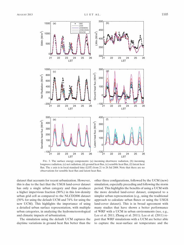
dataset that accounts for recent urbanization. However,

this is due to the fact that the USGS land-cover dataset

has only a single urban category and thus produces

a higher impervious fraction (90%) in this low-density

urban grid cell as compared to the NLCD2006 dataset

(50% for using the default UCM and 74% for using the

new UCM). This highlights the importance of using

a detailed urban surface representation, with multiple

urban categories, in analyzing the hydrometeorological

and climatic impacts of urbanization.

The simulation using the default UCM captures the

daytime variations in ground heat flux better than the

other three configurations, followed by the UCM (new)

simulation, especially preceding and following the storm

period. This highlights the benefits of using a UCMwith

the more detailed land-cover dataset, compared to a

simpler urban representation (e.g., using the traditional

approach to calculate urban fluxes or using the USGS

land-cover dataset). This is in broad agreement with

many studies that have shown a better performance

of WRF with a UCM in urban environments (see, e.g.,

Lee et al. 2011; Zhang et al. 2011). Lee et al. (2011) re-

port that WRF simulations with a UCM are better able

to capture the near-surface air temperature and the

FIG. 3. The surface energy components: (a) incoming shortwave radiation, (b) incoming

longwave radiation, (c) net radiation, (d) ground heat flux, (e) sensible heat flux, (f) latent heat

flux. The x axis is in local standard time (LST) from 21 to 26 Jul 2008. Note that there are no

observations for sensible heat flux and latent heat flux.


atmospheric boundary layer height in urban areas.

Zhang et al. (2011) found that a UCM is needed in order

to correctly reproduce the land surface temperature

patterns or the urban heat island effects. However, we

also cautiously note that the measured ground heat flux

is a point measurement while the simulated ground heat

flux is an average value for the grid cell. As such, the

comparison between the new and default UCM based

only on the ground heat flux remains inconclusive. We

are currently conducting additional analyses using more

representative experimental datasets to assess the per-

formance of the new UCM scheme comprehensively.

The surface meteorological conditions are also ex-

amined by comparing WRF simulations to the obser-

vations at the CubHill tower site. As shown in Fig. 4, it is

clear that the discrepancies between the WRF results

and observations are generally larger during the heavy

rainfall period (from 22 July to 24 July). For example,

the wind speeds produced by WRF are substantially

larger than the measurements. The peak in specific hu-

midity occurred during the late evening of 22 July in

WRF simulations but in the middle of the day on 23 July

in the observations. This time lag in the peak values of

specific humidity between WRF simulations and the

observations is related to discrepancies in the wind field.

As shown in Fig. 4d, there is a phase error in the wind

direction comparison between theWRF simulations and

the observations. The southerly winds (from 908 to 2708)occurred earlier inWRF (midday on 22 July) than in the

observation (midnight on 22 July to early morning on 23

July). The southerly and southeasterly winds are the

main agents for transporting moist air. As a result, the

fact that the southerly winds occurred much earlier in

WRF simulations causes the peak value in the specific

humidity to appear earlier in the WRF simulations than

in the observations. For air temperature,WRF performs

poorly during rainfall periods. During these periods, the

range of air temperatures from WRF is limited com-

pared to the observations, that is, WRF temperature is

much colder in the daytime (by up to 8K) and hotter in

the nighttime (by up to 3K). While the air temperature

measurements may have relatively larger uncertainties

under heavy rainfall conditions, this discrepancy is more

likely to be related to the fact that WRF does not cap-

ture rainfall fields correctly, as will be shown later. For

example, in the late afternoon on 23 July, WRF started

to generate rainfall, which was absent in the observa-

tions, and hence, the air temperature in WRF was al-

most 5K lower than the observations.

Comparisons of 2-m air temperature and specific hu-

midity measured by ASOS at BWI, NAK, and DMH

(locations shown in Fig. 1) showed similarities in the

FIG. 4. (a) Specific humidity, (b) air temperature, (c) wind speed, and (d) wind direction

measured and simulated at the Cub Hill tower (41.2m above the ground level). The x axis is in

LST from 21 to 26 Jul 2008.


magnitudes and timing patterns of errors (not shown

here).

b. Vertical atmospheric profiles

In this section, vertical profiles of potential tempera-

ture, specific humidity, wind speed, and wind direction

from WRF simulations at 1200 UTC (0700 LST) are

compared to radiosonde measurements at the APG

(in d03) site throughout the rainfall event (from 21 to 24

July). As shown in Fig. 5, it is clear that the vertical

profiles of potential temperature, specific humidity, and

winds are not highly sensitive to the urban surface rep-

resentations. The vertical profiles on 21 and 24 July

agree well with the measurements (to a lesser extent for

specific humidity) since they are less affected by the

heavy rainfall event, implying good model skill of WRF

under nonrainy conditions. On 22 July, the agreement

between the measured and simulated profiles is still

good for potential temperature and specific humidity

(note that the agreement is even improved for specific

humidity in the upper atmosphere as compared to 21

and 24 July), but the errors are large for wind speed and

direction. In particular, the jetlike structure at around

700 hPa is missed by all WRF simulations. On 23 July

(about 12 h before the heavy rainfall event), all profiles

from WRF deviate significantly from the measured

ones, especially in the lower atmosphere and especially

for winds. The lower part of the atmosphere is drier and

colder in WRF simulations. The local maximum in wind

speed profile at about 550 hPa is not well reproduced by

WRF. Unlike the jetlike structure observed on 22 July,

the one formed on 23 July has a much stronger southerly

component that brings moisture into the Baltimore re-

gion. In addition, the observed winds in the atmospheric

FIG. 5. Vertical profiles of potential temperature, specific humidity, wind speed and wind direction at the APG site during the heavy

rainfall period: (a) 21 Jul, (b) 22 Jul, (c) 23 Jul, (d) 24 Jul. Profiles are all at the time of the sounding: 1200 UTC (0700 LST).


boundary layer (below 850 hPa) on 23 July are easterly

and transport moisture from the Atlantic Ocean, while

the winds from WRF simulations are southerly or south-

westerly. As a result, the discrepancies in the wind fields

(both wind speed and wind direction) may result in

significant biases in the moisture fields and thus in the

simulated rainfall fields.

Fig. 6 compares the potential temperature and water

vapormixing ratio profiles in the lower atmosphere from

the reference WRF simulation (case 1) to the ACARS

measurements at IAD (d02). Good agreement is seen

for potential temperature (Fig. 6a,b), but WRF pro-

duces a moister atmospheric boundary layer compared

to the ACARS measurements (Fig. 6c,d). Fig. 7 shows

FIG. 6. Evolution of (a),(b) potential temperature and (c),(d) water vapor mixing ratio in the lower atmosphere (up to 4 km above the

ground level) at IAD: (a),(c) aircraft measurements and (b),(d) results with the reference WRF simulation (case 1: WSM6 1 UCM).

FIG. 7. Composite profiles of (left) potential temperature and (right) water vapor mixing ratio in the lower atmosphere (up to 4 km

above the ground level) at IAD: (a),(d) prestorm (0000 UTC 21 Jul to 0000 UTC 22 Jul); (b),(e) in-storm (0000 UTC 22 Jul to 1200 UTC

24 Jul); and (c),(f) after-storm conditions (1200 UTC 24 Jul to 0000 UTC 26 Jul).


the composite profiles of potential temperature and

water vapormixing ratio for the three periods: prestorm,

storm, and after storm. It is clear that the composite

potential temperature profiles from the WRF simula-

tionsmatch theACARSmeasurements better above the

atmospheric boundary layer than in the atmospheric

boundary layer. The bias is about 1–2K in the atmo-

spheric boundary layer during the prestorm period. The

largest bias occurs at the surface (about 2.5K) and is

caused by the errors in the initial conditions that are

taken from NARR. Above the atmospheric boundary,

the agreement is very good, except during the storm

period when the bias is about 1K. While the composite

temperature profiles from the WRF simulation are in

relatively good agreement with the ACARS measure-

ments, the composite water vapor mixing ratio profiles

show larger discrepancies. Before and during the storm,

the lower atmosphere in the WRF simulations is con-

sistently 1–2 g kg21 moister than the observations. This

is consistent with the simulated overestimation of rain at

IAD (e.g., compared to the radar observation, as will be

shown in Fig. 14). After the storm, the composite water

vapor mixing ratio profiles from the WRF simulations

correspond to the measured ones, implying that the

biases in the water vapor profiles are primarily associ-

ated with the initial conditions (provided by NARR) as

well as the development of storm conditions.

Different urban surface representations examined in

this study do not alter the results significantly, except

close to the surface where land–atmosphere exchanges

play a significant role. Differences between simulations

with different surface parameterizations are an order of

magnitude smaller than differences between theseWRF

runs and observations. Theseminor differences between

simulations with different urban surface representations

are largely seen in the atmospheric boundary layer and

are connected to the different surface fluxes and rainfall

fields generated by the different representations. Similar

comparisons (cf. Fig. 6 and Fig. 7) were also conducted

at BWI (d03), where only measurements of potential

temperature are available. As at IAD, the simulated

potential temperature profiles fromWRFalsomatch the

ACARS measurements at BWI fairly well (not shown

here): the bias is larger in the atmospheric boundary

layer than above the atmospheric boundary layer, and

the largest bias occurs at the surface because of the er-

rors in the initial conditions. The differences between

WRF-simulated boundary layer profiles with different

urban surface representations are also minor.

The velocity–azimuth display (VAD) wind profiles

derived from Doppler velocity measurements at three

locations, KLWX, KAKQ, and KCCX, are compared to

the WRF-simulated results (the reference simulation,

case 1) from d01. Other WRF simulations with different

physical parameterizations were also examined and

similar features were observed (not shown). KLWX

(KAKQ) are located southeast (south) of the Baltimore–

Washington metropolitan area (see Fig. 1) and thus are

selected to capture the southerly jet flow features in the

wind profiles (Figs. 8a,b and Fig. 9). KCCX is located

northwest of the Baltimore–Washington metropolitan

area and is suitable for identifying errors associated

with development of the storm system (Figs. 8c,d and

Fig. 10).

A notable feature in the VAD data at KLWX (Figs.

8a,b) is a strong southerly jet ranging from about 500 to

4000m above the ground that starting on 23 July. The

magnitude of the jet is significantly underestimated by

the WRF simulation. The low-level jet feature observed

in the wind profiles deserves investigation since many

studies have demonstrated the role of LLJs in trans-

porting warm, moist air in the lower atmosphere and

their close relation with heavy rainfall (Zhang and

Fritsch 1986; Stensrud 1996; Higgins et al. 1997; Zhang

et al. 2006). According to Zhang et al. (2006), a low-level

jet can be broadly defined as a region below 1500m with

wind speeds larger than 12m s21, positive shear below,

and negative shear above. In other words, a local max-

imum wind speed below 1500m that is stronger than

12m s21 can be viewed as an indicator of low-level jets.

Fig. 9 shows the maximum wind below 1500m (above

ground level) and its direction at KLWX and KAKQ

from the VAD data and the WRF simulation. The

horizontal dashed lines in Figs. 9a and 9c show the

threshold value of 12ms21 above which an LLJ is iden-

tified. The correlation coefficient, root-mean-square er-

ror (RMSE), andmean bias between theWRF-simulated

and radar-observed values are shown in Table 2. Note

that when calculating these metrics for wind direction,

the WRF-simulated or radar-observed values some-

times need to be adjusted (i.e., adding 3608). In general,

the WRF simulation captures the variations in the max-

imum wind speed below 1500m with correlation co-

efficients of 0.65 at the two locations. The RMSEs are

2.8 and 2.9m s21 for KLWX and KAKQ, respectively.

The WRF simulation also captures the general varia-

tions in the wind direction of the maximum wind speed

at KLWX, with the RMSE and the mean bias of 39.58and 2.88, respectively. From Figs. 9a and 9b, it is clear

that a low-level jet is present in VAD measurements on

23 July at KLWX (themaximumwind speed is above the

horizontal dashed line). Its direction is captured in the

model simulations, but its strength is underestimated.

This is consistent with the comparison in Figs. 8a and 8b.

The low-level jet has a southwesterly component (wind

direction ranging from 1808 to 2708) and thus transports


warmer and moister air from the south to the Baltimore

metropolitan area.

The RMSE and the mean bias between the simulated

and measured wind direction of the maximum wind

speed are roughly twice as large at KAKQ (66.58 and26.18, respectively). As can be seen fromFigs. 9c and 9d,

at KAKQ, two low-level jets are formed, one around

0300 UTC 23 July and the other around 0000 UTC

24 July. The first low-level jet is more significant than the

second one, but it is not well reproduced by the WRF

simulation with an underestimation of its magnitude and

duration. More importantly, the direction associated with

this low-level jet is significantly biased by the WRF

simulation leading up to the storm period. The observed

wind direction veers steadily from about 0000 UTC

22 July to about 1200 UTC 23 July, while the WRF re-

mains roughly constant around 3008. The easterly com-

ponent (wind direction ranging from 0 to 1808) of the

low-level jet is not captured by the WRF simulation,

which corresponds with the comparison of radiosonde

profiles at APG (Fig. 5c). Note both APG and KAKQ

are located along the Chesapeake Bay or the coast. As

such, misrepresentation of the easterly low-level jet at

these two sites in WRF simulations implies incorrect

FIG. 8. Horizontal wind speed and direction at (a),(b) KLWX and (c),(d) KCCX in the lower atmosphere from the (a),(c) VAD wind

profiles and (b),(d) reference WRF simulation (case 1: WSM6 1 UCM). The colors indicate the wind speed magnitude (m s21) and the

arrows are the wind direction in the horizontal plane: x axis is the west–east direction while y axis is the north–south direction. The heights

are above sea level and are at intervals of 250m.


moisture transport from the Atlantic Ocean, which fur-

ther results in incorrect rainfall amounts and distribution.

Comparisons of the wind profiles from the model

simulation to the VAD data at KCCX (Figs. 8c,d) show

that WRF captures the broad features of variation in

wind direction. From the composite wind speed and

wind direction shown in Fig. 10, it can be seen that be-

fore the storm period, the wind is primarily from the

FIG. 9. Comparison of the maximum wind (a),(c) speed and (b),(d) direction below 1500m (above ground level) at (a),(b) KLWX and

(c),(d) KAKQ from VAD data and the reference WRF simulation (case 1: WSM61UCM). The horizontal dashed lines in (a),(c) show

the threshold value of 12m s21.

FIG. 10. Composite profiles of wind (a)–(c) speed and (d)–(f) direction at (a),(d) KCCX prestorm (0000 UTC 21 Jul to 0000 UTC 22 Jul);

(b),(e) in-storm (0000 UTC 22 Jul to 1200 UTC 24 Jul); and (c),(f) after-storm conditions (1200 UTC 24 Jul to 0000 UTC 26 Jul).


northwest, while during and after the storm, southerly

flows are observed. However, WRF systematically over-

estimates the wind speed, in particular before the storm

and during the storm (Figs. 10b,c). Because KCCX is

located to the northwest of Baltimore City, the errone-

ously large northwesterly winds before the storm period

in the model simulation are linked to erroneous rapid

motion of the frontal zone toward the Baltimore metro-

politan area. As will be seen later, the excessively rapid

frontal circulation and movement toward the southeast

causes the rainfall event to occur about 4h ahead of the

observations in the Baltimore metropolitan area.

c. Rainfall

In this section, we analyze the biases inWRF-simulated

precipitation and link them to the biases in atmo-

spheric dynamics analyzed in the previous section. The

rainfall rates simulated by WRF (domain 3), observed

by the high-resolution radar dataset, and provided by

the coarse-resolution NARR dataset are averaged and

compared over their overlap region. As mentioned be-

fore, the high-resolution radar rainfall dataset covers

a large part of the Baltimore metropolitan area, with

a temporal resolution of 15min and a spatial resolution

of 1 km. The NARR dataset covers the whole North

American continent, with a temporal resolution of 3 h

and a spatial resolution of 32 km. WRF fields from d03

have a temporal resolution of 1 h and a spatial resolution

of 1 km. For comparison with WRF, the radar rainfall

estimates are averaged into hourly intervals. As can be

seen from Fig. 11, the radar observations and theNARR

dataset indicates that the rainfall event in d03 started

around 0000 UTC 24 July. Note the peak rainfall in the

NARR dataset is significantly reduced as compared to

the radar observations due to its coarser temporal res-

olution. It is clear that the WRF simulations do not

capture the correct timing of the heavy rainfall event.

The rain event simulated by WRF occurred about 4 h

earlier than the radar observations. As mentioned ear-

lier, the time lags between WRF simulations and the

radar observations are primarily linked to the faster

development of the front, which is further illustrated in

Fig. 12.

Fig. 12 compares the 2-m specific humidity fields and

surface wind fields from the NARR dataset to those

from the reference WRF simulation (case 1: WSM6 1UCM) in domain 1 at four times, from 1800UTC 23 July

to 0300 UTC 24 July. As mentioned earlier, the frontal

boundary passes the Baltimore–Washington area at

0000 UTC 24 July in the NARR data, as shown by the

bold white dotted line in Fig. 12e. Nonetheless, theWRF

model fields show that the frontal boundary passed the

Baltimore–Washington corridor at 2100 UTC 23 July

(Fig. 12d). This is in agreement with the higher (com-

pared to observations) wind speed simulated at KCCX,

a location that is behind the front (see Fig. 10). As a re-

sult, WRF generates rainfall in the Baltimore metro-

politan area approximately 4 h earlier than in the

NARR and radar rainfall fields. This feature is similar to

the results of Miao et al. (2011) who show that the

modeled convergence line in their summer rainfall case

TABLE 2. Comparison between WRF-simulated and radar-

observed LLJs.

Variables Correlation RMSE Mean bias

KLWX Wind speed 0.65 2.8m s21 0.2m s21

Wind direction 0.66 39.58 2.88KAKQ Wind speed 0.65 2.9m s21 20.7m s21

Wind direction 0.75 66.58 26.18

FIG. 11. Time series of rainfall rate averaged over the Baltimore metropolitan area (d03) from

1200 UTC 23 Jul to 1200 UTC 24 Jul.


FIG. 12. The 2-m specific humidity (colors) and 10-m winds (arrows) in d01 at: (top row) 1800 and (second row)

2100UTC on 23 Jul; and (third row) 0000 and (bottom row) 0300UTC on 24 Jul fromNARRand the referenceWRF

simulation (case 1: WSM61 UCM). The black square surrounding the Baltimore metropolitan area is d03 in WRF

simulations. The bold white dotted lines roughly indicate the frontal boundary locations.


(1 August 2006, Beijing) moves more rapidly than the

observed one. Zhang et al. (2009) also observed that the

cold front simulated by WRF in their study moves too

fast compared with observations. In addition, they also

reported that this bias is not alleviated by changing the

boundary conditions (i.e., the forcing data).

In addition, the strength of the moisture gradient is

significantly different in the WRF simulation than in

NARR at the time when the frontal boundary passes the

Baltimore area. The cold front generated by the WRF

simulation is significantly drier than that in the NARR

data. The Chesapeake Bay region also has a lower

moisture content, which is consistent with our previous

finding that WRF does not capture the easterly flow

component that transports moisture from the Atlantic

Ocean (as mentioned earlier for comparisons at APG

and KAKQ; see Figs. 5c and 9). The lack of an easterly

flow along the coast in WRF simulations may also in-

directly contribute to the more rapidly moving frontal

boundary.

Figure 11 also illustrates the sensitivity of heavy

rainfall in WRF to different urban representations and

microphysics schemes. The large sensitivity to urban

representations is of particular interest. Fig. 13 further

illustrates the impact of urban representations on the

spatial distribution of total rainfall occurring during 23

and 24 July at a high spatial resolution (1 km). The dif-

ferences in total rainfall between three cases that use

three different urban surface representations (cases 3, 4,

and 5 in Table 1) and the control case (case 1 in Table 1)

are depicted in Figs. 13b–d. Figure 13a also shows

the urban land-use categories in domain 3 from the

NLCD2006 date set. As can be seen in Figs. 13b–d,

changes in urban surface representations (including

FIG. 13. The sensitivities of total rainfall from 23 to 24 Jul (1200–1200 UTC) in d03 to the urban surface repre-

sentations in WRF. (a) Land-cover map in d03 and total rainfall difference (%) between: (b) case 3 (new UCM,

NLCD2006) and case 1; (c) case 4 (defaultUCM,USGS) and case 1; and (d) case 5 (noUCM,NLCD2006) and case 1.

The reference case 1 uses the default UCM with NLCD2006 dataset. The black dots indicate Baltimore City.


changes in the urban flux calculation methods and

changes in the land-cover datasets) can result in local

differences in total rainfall of more than 150%. The

main difference is that the impervious surface fraction

and the vegetated surface fraction differ as a result of

land-use dataset and UCM selection. For example, a

large part of suburban areas around Baltimore and

Washington are classified as low-intensity urban land

and, thus, a 50% impervious surface fraction is assigned

for each grid in the default UCM. In the new UCM, the

fraction of impervious surface is calculated directly from

NLCD2006, and it tends to exceed 50% around the two

cities. The USGS dataset–based run will treat all urban

areas as high density with 90% impervious fraction.

When no UCM is used, all of the urban areas will be

treated exclusively as impervious surfaces. As the im-

pervious surface fraction increases, more available en-

ergy is converted into sensible heat flux, which leads to

changes in local convection regimes. As the impervious

surface fraction increases, more rainfall is generated

along the Baltimore–Washington corridor in response

to the increases in the sensible heat fluxes, while a belt

with reduced rain is produced to the northwest of the

urban areas (Fig. 13).

Figure 14 shows the total rainfall from 23 to 24 July

(1200–1200 UTC) derived from the KLWX radar and

produced by different WRF simulations over a large

domain in order to illustrate the sensitivities of large-

scale rainfall patterns to microphysics and urban sur-

face representations. From the radar measurement, it is

clear that most of the rain is concentrated northeast of

the Baltimore metropolitan region (downwind of the

urban region; see Smith et al. 2012). Observational

studies that have focused on the impact of urbanization

on precipitation have shown that warm seasonal rain-

fall consistently shows a local maximum downwind of

major cities [see Shephard (2005) for a review and Smith

et al. (2012) for analyses in the Baltimore region].

However,WRF does not generate themaximum rainfall

at the correct location for this event. Based on the pre-

vious analyses, this is caused by the biases in the WRF-

simulated wind fields, which further leads to biases in

the moisture transport. The maximum rainfall in WRF

simulations occur more inland as compared to the radar

FIG. 14. The total rainfall from 23 to 24 Jul (1200–1200UTC) (a)measured by the KLWX radar and (b)–(f) produced byWRF simulations

with different microphysics and urban surface representations as indicated in the lower right corner of each panel.


observation, which is in agreement with the weaker

easterly flow along the Chesapeake Bay or the coast that

was observed in section 3b. The faster-moving fron-

tal boundary toward the southeast also contributes to

changes in the maximum rainfall location in WRF sim-

ulations. In addition, WRF simulations produce the two

parallel line structures in the rainfall fields, but generate

too much rainfall in each line. This overestimation of

rainfall by WRF is also in agreement with many pre-

vious studies (see, e.g., Yeung et al. 2011) and is also

caused by incorrect moisture transport. Changes in mi-

crophysics schemes alter the spatial structure of the

rainfall field, but more sophisticated microphysics pa-

rameterizations (WDM6) do not generate better results

as compared to radar observations.

It is interesting to observe from Fig. 14 that the large-

scale rainfall fields are clearly as sensitive to the urban

surface representations as to the microphysics schemes.

The fact that large-scale rainfall fields are affected

by urban surface representations suggests a potentially

significant role of urbanization in modifying regional

precipitation patterns. More importantly, it also sug-

gests that studies using numerical tools such as WRF to

investigate the impact of urbanization on precipitation

need to be more careful in selecting urban surface rep-

resentations. In addition, the significant sensitivity of

rainfall structure to urban surface representations ob-

served in our study demonstrates a strong need for ac-

curate characterizations of urban surfaces in numerical

weather prediction models.

4. Conclusions

In this study, we examine the role of land surface

processes in modulating heavy rainfall in the Baltimore–

Washington metropolitan region and the role of heavy

rainfall in controlling land surface processes and the

structure of the atmospheric boundary layer. Analyses

are based on comparisons of high-resolution WRF model

fields with a broad range of observations. The perfor-

mance of WRF and sensitivities to urban surface pa-

rameterizations andmicrophysics schemes are examined.

The main conclusions are as follows:

1) The urban surface representation is a key determi-

nant of the surface energy balance in urban environ-

ment. The UCM with the high-resolution NLCD2006

land-cover dataset captures the surface energy par-

titioning reasonably well at the Cub Hill tower site

(a low-density residential area). The UCM with the

default USGS land-cover dataset case and the no-

UCM case, which have higher impervious fractions,

yield larger sensible and ground heat fluxes and

smaller latent heat fluxes compared to the control

simulation. As the urban surface representation more

accurately reflects the vegetated/impervious frac-

tions, the calculation of land–atmosphere exchanges

becomes more accurate, yet it remains inconclusive

whether adding grid-scale complexity via the new

UCM yields further improvement.

2) The surface microclimate conditions are generally

well reproduced byWRF. During the rainfall period,

however, WRF generates large biases in air temper-

ature, specific humidity, and the wind field. These

biases are closely associated with the discrepancies in

the WRF-modeled rainfall field such as the over-

estimation of the inland rainfall and the incorrect

timing of the rainfall event.

3) Large biases are observed in the WRF-simulated

wind field in the lower atmosphere:WRF simulations

do not fully capture the jetlike structures that are

main agents for moisture transport. WRF simula-

tions also produce stronger northwesterly winds that

move the frontal boundary faster than in the obser-

vations. The agreement between WRF-simulated

and measured vertical profiles is good for potential

temperature and specific humidity preceding and

following the heavy rainfall period, but less satisfac-

tory during the storm when the simulated atmo-

spheric boundary layer is considerably moister than

the observed one.

4) WRF simulations reproduce the inland linear pat-

terns of rainfall but generate too much precipitation

along these lines and not enough precipitation else-

where, particularly farther downwind of the urban

areas (along the Chesapeake Bay). In addition,WRF

does not capture the correct timing for the passage

of the frontal system, which results in a time lag

between the simulated and observed rainfall fields.

5) Both urban surface representations andmicrophysics

schemes in WRF affect heavy rainfall modeling sig-

nificantly. In particular, the sensitivity of spatial

rainfall structures and the spatially averaged time

series of rainfall rate to urban surface representation

are comparable to the sensitivity to the microphysics

scheme examined in our study, demonstrating that

inclusion of urban physics is important for WRF and

other numerical weather prediction models to cap-

ture heavy rainfall.

The significant role of urban surface representations

in modulating urban-atmosphere exchanges, atmo-

spheric boundary layer structures, and rainfall distri-

bution has many implications. First, it demonstrates the

importance of developing an urban modeling system

that captures the key finescale processes that occur in


urban environments and coupling it to the large-scale

numerical weather and climate models (Chen et al.

2011). Second, it suggests that choice of urban repre-

sentation in theWRFmodel, like the choice of any other

physical parameterization, plays a significant role in

rainfall modeling. Studies that rely on numerical tools

such as WRF to assess the impact of urbanization on

rainfall need to give careful consideration to the choice

of urban surface representation.

The current study does have some limitations that are

important to appreciate. First of all, the conclusions are

drawn based on analyses of a single heavy-rainfall event.

More precipitation events of different types and under

different forcing conditions should be investigated to

overcome the limitation of a case study. Second, some

analyses such as the validation of surface radiative and

turbulent fluxes are based on limited measurements.

More experimental datasets will be used in future work

to assess the performance of different urban surface

representations. In addition, some of the biases ob-

served in this study are not isolated from the un-

certainties in the initial and boundary conditions, which

were provided by the NARR dataset. Future work in-

volves using other forcing datasets in addition to NARR

to help identify the biases that are generated by WRF

itself. This paper also identifies several limitations in the

WRF modeling system that improvements to the urban

parameterization may not address, such as the biases in

the WRF wind fields that cause a faster development of

the front. Further efforts are also needed to address

these limitations in order to improve the predictability

of WRF at large and to use WRF for other environ-

mental and hydrological applications.

Acknowledgments. This work is supported by the NSF

under Grant CBET-1058027 and by the Mid-Infrared

Technology forHealth and the Environment (MIRTHE)

NSF Engineering Research Center at Princeton Uni-

versity under Grant EEC-0540832. The simulations

were performed on the supercomputing clusters of the

National Center for Atmospheric Research and of

Princeton University. We are grateful to Drs. JohnHom

and Nicanor Saliendra from the Forest Service of the

U.S. Department of Agriculture for providing us with

themeanmeteorological observations from theCubHill

tower. We also thank Yinzhen Jin and Long Yang for

their help in processing the VAD data and Ting Sun for

processing the figures.

REFERENCES

Ashley, W. S., M. L. Bentley, and J. A. Stallins, 2012: Urban-

induced thunderstorm modification in the southeast United

States. Climatic Change, 113, 481–498.

Betts, A. K., J. H. Ball, A. C. M. Beljaars, M. J. Miller, and P. A.

Viterbo, 1996: The land surface-atmosphere interaction: A

review based on observational and global modeling perspec-

tives. J. Geophys. Res., 101, 7209–7225.Bornstein, R., and Q. L. Lin, 2000: Urban heat islands and sum-

mertime convective thunderstorms in Atlanta: Three case

studies. Atmos. Environ., 34, 507–516.Brutsaert, W., 2005: Hydrology: An introduction. Cambridge Uni-

versity Press, 605 pp.

Chen, F., and Coauthors, 2011: The integrated WRF/urban mod-

elling system: Development, evaluation, and applications

to urban environmental problems. Int. J. Climatol., 31, 273–

288.

Dixon, P. G., and T. L.Mote, 2003: Patterns and causes ofAtlanta’s

urban heat island-initiated precipitation. J. Appl. Meteor., 42,

1273–1284.

Higgins, R.W., Y. Yao, E. S. Yarosh, J. E. Janowiak, andK. C.Mo,

1997: Influence of the Great Plains low-level jet on summer-

time precipitation and moisture transport over the central

United States. J. Climate, 10, 481–507.

Hong, S. Y., and J. J. Lim, 2006: The WRF Single-Moment 6-Class

Microphysics Scheme (WSM6). J. Korean Meteor. Soc., 42,

129–151.

——, K. S. Lim, Y. H. Lee, J. C. Ha, H. W. Kim, S. J. Ham, and

J. Dudhia, 2010: Evaluation of the WRF Double-Moment

6-Class Microphysics Scheme for Precipitating Convection.

Adv. Meteor., 2010, 707253, doi:10.1155/2010/707253.Jankov, I., W. A. Gallus, M. Segal, B. Shaw, and S. E. Koch, 2005:

The impact of different WRF model physical parameteriza-

tions and their interactions on warm season MCS rainfall.

Wea. Forecasting, 20, 1048–1060.Jiang, X. Y., C. Wiedinmyer, F. Chen, Z. L. Yang, and J. C. F. Lo,

2008: Predicted impacts of climate and land use change on

surface ozone in the Houston, Texas, area. J. Geophys. Res.,

113, D20312, doi:10.1029/2008JD009820.

Jin, M. L., and J.M. Shepherd, 2008: Aerosol relationships to warm

season clouds and rainfall at monthly scales over east China:

Urban land versus ocean. J. Geophys. Res., 113, D24S90,

doi:10.1029/2008JD010276.

——, ——, and W. Z. Zheng, 2010: Urban surface temperature

reduction via the urban aerosol direct effect: A remote sensing

andWRFmodel sensitivity study.Adv. Meteor., 2010, 681587,

doi:10.1155/2010/681587.

Krajewski, W. F., and Coauthors, 2011: Towards better utilization

of NEXRAD data in hydrology: An overview of Hydro-

NEXRAD. J. Hydroinformatics, 13, 255–266.

Lee, S. H., and Coauthors, 2011: Evaluation of urban surface pa-

rameterizations in the WRF model using measurements dur-

ing the Texas Air Quality Study 2006 field campaign. Atmos.

Chem. Phys., 11, 2127–2143.

Lim, K. S. S., and S. Y. Hong, 2010: Development of an effective

double-moment cloud microphysics scheme with prognostic

cloud condensation nuclei (CCN) for weather and climate

models. Mon. Wea. Rev., 138, 1587–1612.Lin, C. Y., W. C. Chen, P. L. Chang, and Y. F. Sheng, 2011: Impact

of the urban heat island effect on precipitation over a complex

geographic environment in northern Taiwan. J. Appl. Meteor.

Climatol., 50, 339–353.

Loose, T., and R. D. Bornstein, 1977: Observations of mesoscale

effects on frontal movement through an urban area. Mon.

Wea. Rev., 105, 563–571.Miao, S. G., F. Chen,Q. C. Li, and S. Y. Fan, 2011: Impacts of urban

processes and urbanization on summer precipitation: A case


study of heavy rainfall in Beijing on 1 August 2006. J. Appl.

Meteor. Climatol., 50, 806–825.

Niyogi, D., and Coauthors, 2011: Urban modification of thunder-

storms: An observational storm climatology and model case

study for the Indianapolis urban region. J. Appl. Meteor. Cli-

matol., 50, 1129–1144.

Ntelekos, A. A., J. A. Smith, and W. F. Krajewski, 2007: Cli-

matological analyses of thunderstorms and flash floods

in the Baltimore metropolitan region. J. Hydrometeor., 8,

88–101.

——, ——, M. L. Baeck, W. F. Krajewski, A. J. Miller, and

R. Goska, 2008: Extreme hydrometeorological events and the

urban environment: Dissecting the 7 July 2004 thunderstorm

over the Baltimore MD metropolitan region. Water Resour.

Res., 44, W08446, doi:10.1029/2007WR006346.

——,——, L. Donner, J. D. Fast, W. I. Gustafson, E. G. Chapman,

and W. F. Krajewski, 2009: The effects of aerosols on intense

convective precipitation in the northeastern United States.

Quart. J. Roy. Meteor. Soc., 135, 1367–1391.Pielke, R. A., 2001: Influence of the spatial distribution of vege-

tation and soils on the prediction of cumulus convective

rainfall. Rev. Geophys., 39, 151–177.

Rosenfeld, D., 2000: Suppression of rain and snow by urban and

industrial air pollution. Science, 287, 1793–1796.

Shem, W., and M. Shepherd, 2009: On the impact of urbanization

on summertime thunderstorms in Atlanta: Two numerical

model case studies. Atmos. Res., 92, 172–189.

Shephard, J. M., 2005: A review of current investigations of urban-

induced rainfall and recommendations for the future. Earth

Interact., 9. [Available online at http://EarthInteractions.org.]

Shepherd, J. M., M. Carter, M. Manyin, D. Messen, and S. Burian,

2010: The impact of urbanization on current and future coastal

precipitation: a case study for Houston. Environ. Plann., 37B,

284–304.

Skamarock, W. C., and J. B. Klemp, 2008: A time-split non-

hydrostatic atmospheric model for weather research and

forecasting applications. J. Comput. Phys., 227, 3465–3485.Smith, J. A., M. L. Baeck, G. Villarini, C. Welty, A. J. Miller, and

W. F. Krajewski, 2012: Analyses of a long-term, high-resolution

radar rainfall data set for the Baltimore metropolitan region.

Water Resour. Res., 48, W04504, doi:10.1029/2011WR010641.

Stensrud, D. J., 1996: Importance of low-level jets to climate: A

review. J. Climate, 9, 1698–1711.

Talbot, C., E. Bou-Zeid, and J. Smith, 2012: Nested mesoscale

large-eddy simulations with WRF: Performance in real test

cases. J. Hydrometeor., 13, 1421–1441.

Trier, S. B., F. Chen, and K. W. Manning, 2004: A study of con-

vection initiation in a mesoscale model using high-resolution

land surface initial conditions.Mon.Wea. Rev., 132, 2954–2976.

——,——,——,M. A. LeMone, and C. A. Davis, 2008: Sensitivity

of the PBL and precipitation in 12-day simulations of warm-

season convection using different land surface models and soil

wetness conditions. Mon. Wea. Rev., 136, 2321–2343.

——,M.A. LeMone, F. Chen, andK.W.Manning, 2011: Effects of

surface heat and moisture exchange on ARW-WRF warm-

season precipitation forecasts over the central United States.

Wea. Forecasting, 26, 3–25.

Wang, Z. H., E. Bou-Zeid, S. K. Au, and J. A. Smith, 2011: Ana-

lyzing the sensitivity of WRF’s single-layer urban canopy

model to parameter uncertainty using advanced Monte Carlo

simulation. J. Appl. Meteor. Climatol., 50, 1795–1814.——, ——, and J. A. Smith, 2013: A coupled energy transport and

hydrological model for urban canopies evaluated using

a wireless sensor network. Quart. J. Roy. Meteor. Soc.,

doi:10.1002/qj.2032, in press.

Wood, E. F., and Coauthors, 2011: Hyperresolution global land

surface modeling: Meeting a grand challenge for monitoring

Earth’s terrestrial water. Water Resour. Res., 47, W05301,

doi:10.1029/2010WR010090.

Wright, D. B., J. A. Smith, G. Villarini, and M. L. Baeck, 2012:

Hydroclimatology of flash flooding in Atlanta. Water Resour.

Res., 48, W04524, doi:10.1029/2011WR011371.

Yeung, J. K., J. A. Smith, G. Villarini, A. A. Ntelekos,M. L. Baeck,

and W. F. Krajewski, 2011: Analyses of the warm season

rainfall climatology of the northeastern US using regional

climatemodel simulations and radar rainfall fields.Adv.Water

Resour., 34, 184–204.

Zhang, D. L., and J. M. Fritsch, 1986: Numerical simulation of the

meso-b scale structure and evolution of the 1977 Johnstown

Flood. Part I: Model description and verification. J. Atmos.

Sci., 43, 1913–1943.

——, S. L. Zhang, and S. J. Weaver, 2006: Low-level jets over the

Mid-Atlantic states: Warm-season climatology and a case

study. J. Appl. Meteor. Climatol., 45, 194–209.

——, Y. X. Shou, R. R. Dickerson, and F. Chen, 2011: Impact of

upstream urbanization on the urban heat island effects along

the Washington–Baltimore corridor. J. Appl. Meteor. Clima-

tol., 50, 2012–2029.

Zhang, Y., J. A. Smith, A. A. Ntelekos, M. L. Baeck, W. F.

Krajewski, and F. Moshary, 2009: Structure and evolution

of precipitation along a cold front in the northeastern United

States. J. Hydrometeor., 10, 1243–1256.


modeling land surface processes and heavy rainfall in

Documents