Aalto UniversitySchool of ScienceDegree programme in Engineering Physics and Mathematics

Modeling space elasticity of demand tosupport retail replenishment planning

Bachelor’s thesisJune 11, 2018

Tommi Vainio

The document can be stored and made available to the public on the openinternet pages of Aalto University.All other rights are reserved.

aalto universityschool of science

abstract of thebachelor’s thesis

Author: Tommi Vainio

Title: Modeling space elasticity of demand to support retail replenishmentplanning

Date: 11.6.2018 Language: English Number of pages: 4+28

Degree programme: Engineering Physics and Mathematics

Major: Mathematics and System Sciences

Supervisor: Prof. Fabricio Oliveira

Advisor: M.Sc. (Econ.) Ville Sillanpää

The demand of a product is affected by the shelf space allocated for it. Thisdependency is called space elasticity and the magnitude of it depends onmultiple product and store-specific attributes. The objective of this thesisis to review the literature related to this relationship between shelf spaceand demand, and develop guidelines with which the space elasticity can beaccurately estimated for a large group of products in multiple stores. Also,ways to utilize the space elasticity information to support retail replenishmentplanning are studied and similar guidelines for optimizing shelf space arepresented.

An important finding regarding the estimation of space elasticity isthat the effect of shelf space is minor compared to other variations in demand.Another significant conclusion is that the products’ position in the shelf, as wellas the store at which the product is sold, affects the space elasticity estimates.Therefore, these two factors need to be controlled when estimating the spaceelasticity values.

Regarding the operational applications of space elasticity information,this thesis concludes that multiple models to optimize shelf space allocationexists, proposing significant profit increases compared to traditional allocationmethods. These models however contain components and assumptions thatcomplicate their application to practical use in large retail chains. Therefore, asimplified model, where profit related to shelf space allocation is maximizedwith restrictions assuring the rationality of the result, is proposed for furtherinvestigation. Using shelf space information to optimize other operations, suchas promotion planning is also proposed to be the subject of future studies.

Keywords: space elasticity, shelf space allocation, decision support

aalto-yliopistoperustieteiden korkeakoulu

kandidaatintyöntiivistelmä

Tekijä: Tommi Vainio

Työn nimi: Kysynnän tilajouston mallintaminen vähittäiskaupantäydennykseen liittyvän päätöksenteon tukena

Päivämäärä: 11.6.2018 Kieli: Englanti Sivumäärä: 4+28

Koulutusohjelma: Teknillinen fysiikka ja matematiikka

Pääaine: Matematiikka ja systeemitieteet

Vastuuopettaja: Prof. Fabricio Oliveira

Työn ohjaaja: KTM Ville Sillanpää

Tuotteen kysyntään vähittäiskaupassa vaikuttaa sen saama hyllytilan määrä.Tätä riippuvuutta kutsutaan kysynnän tilajoustoksi ja sen voimakkuus riippuuuseista tuote- ja myymäläkohtaisista ominaisuuksista. Työn tarkoituksena olikirjallisuuskatsauksen avulla tutkia hyllytilan ja kysynnän välistä yhteyttä sekäkehittää perussääntöjä kysynnän tilajouston luotettavaan arvioimiseen suurellemäärälle tuotteita monissa eri myymälöissä. Tavoitteena oli myös löytää tapojahyödyntää kysynnän tilajoustoa vähittäiskauppojen täydennyksen suunnit-telussa ja tarjota samankaltaiset perussäännöt hyllytilan jakamisen optimointiin.

Tärkeä tulos kysynnän tilajouston estimointiin liittyen oli, että hyllyti-lan vaikutus kysyntään on pieni suhteessa muihin kysyntään vaikuttaviintekijöihin. Tutkimuksessa selvisi myös, että tuotteen sijainti hyllyssä, kutenmyös myymälä, jossa tuotetta myydään, vaikuttavat kysynnän tilajoustollesaataviin arvoihin. Näin ollen nämä tekijät tulee ottaa huomioon tilajoustoaarvioitaessa.

Kysynnän tilajoustotiedon operationaalisen hyödyntämisen suhteen tut-kimuksessa selvisi, että on olemassa useita hyllytilan jakamista optimoiviamalleja, jotka lupaavat merkittäviä lisäyksiä myymälöiden tuottoihin normaalei-hin hyllytilajakoihin verrattuna. Näissä malleissa on kuitenkin ominaisuuksia jaoletuksia, jotka vaikeuttavat niiden hyödyntämistä suurten vähittäiskauppaket-jujen tilanhallinnan jatkuvassa optimoinnissa. Tästä syystä työssä ehdotetaanlisätutkimusten kohteeksi yksinkertaistettua mallia, jossa optimoidaanvain hyllytilajakoon liittyvää tuottoa, ratkaisun järkevyyden varmistavienrajoitusehtojen vallitessa. Työssä ehdotetaan jatkotutkimuksen kohteeksimyös tilajouston hyödyntämistä muissa sovelluksissa, kuten kampanjoidensuunnittelussa.

Avainsanat: kysynnän tilajousto, hyllytilan jako, päätöksenteko

Contents1 Introduction 1

2 Estimating space elasticity 22.1 Depencency between shelf space and demand . . . . . . . . . . 22.2 Significance of store-specific estimation . . . . . . . . . . . . . 72.3 Effect of the position of product . . . . . . . . . . . . . . . . . 112.4 Summary . . . . . . . . . . . . . . . . . . . . . . . . . . . . . 13

3 Using space elasticity information 153.1 Existing optimization models . . . . . . . . . . . . . . . . . . 153.2 Summary . . . . . . . . . . . . . . . . . . . . . . . . . . . . . 21

4 Conclusions 23

A Spatial models 28

1 Introduction

In retailing, the demand of a product is affected by a large number of factors.One of these is the shelf space allocated for the product. If the shelf space ofthe product is increased, consumers are more likely to notice the good andthe product is bought more often. Naturally, it is usually not possible toincrease the shelf space of every product. Therefore, defining the productsand the situations in which the space increases would be beneficial need to bedefined. The demand of different products reacts differently to altering theirshelf space, meaning that products have different space elasticities. This canbe due to multiple factors, such as the category to which the product belongs,location and size of the store it is sold at and numerous other factors. Havingknowledge of how the demand of a product, or product category, will reactto variations in shelf space is useful in making decisions about different storeoperations, such as space allocation, replenishment and promotion planning.

Most retailers acknowledge the space elasticity phenomenon on a general leveland have developed rules of thumb to allocate shelf space, for example so thatthe most popular products, or products having the highest profit margins,get more shelf space. There is however a potential to draw more significantbenefits by determining accurate space elasticity estimates for each productand optimizing different store operations based on this information. How-ever, the problem is that forecasting the effect of shelf space on the demand ofthe product is difficult. The relationship is not similar for every product cat-egory and intuitive dependencies between product attributes and the spaceelasticity are hard to find. The different factors affecting the space elastic-ity of a product have been a subject of investigation in a number of studieswhere different relations between different factors and space elasticities havebeen found. The findings are in some sense consistent, but often ambiguous,which leads to the conclusion that the different factors and relations maynot yet be completely clear. Knowing the space elasticity of a product isin itself useless, if the knowledge is not used to support decision making instore operations. Therefore, multiple studies have been conducted focusingalso on practical use-cases for the space elasticity information. These studiesfocus mainly on different models to optimize shelf space allocation in orderto maximize profit or sales.

This thesis reviews the studied dependencies between different product at-tributes and product’s space elasticity, and aims to find a generally goodway to estimate space elasticities for a large group of SKU’s belonging todifferent categories in different stores. After this, the purpose is to review

2

some of the developed operational applications exploiting the space elastic-ity information. Finally, based on those findings, we determine guidelines forestimation and usage of this information in large retail chains.

2 Estimating space elasticity

2.1 Depencency between shelf space and demand

Curhan [1972] defines the shelf space elasticity as a ratio of the percentagechange in sales to percentage sales in shelf space with a formula

E =(Ct1 − Ct0)/Ct0(St1 − St0)/St0

, (1)

where C is unit sales and S is the shelf space. t0 represent the time period ob-served before the change in the shelf space and t1 is the time period observedafter the change in the shelf space. To study the space elasticity, Curhanconstructed an experiment where he aimed to detect the space elasticity ofdifferent products by altering the shelf space of a sample set of products andmeasuring the unit sales 5 to 12 weeks before or after the change. After this,the author explained the measured elasticities with different variables usinglinear regression. The experiment was conducted with a regional supermar-ket chain. Four of the chain’s stores acted as a test stores where the differentproducts shelf space was altered and 24 other stores of the chain in the samearea were used as control stores. Curhan chose this approach in order to re-move the seasonal, promotional and other variations from sales. In practice,it was done by multiplying the sales of the test product with the ratio of thebase period unit sales to test period unit sales of the control product. Thiswas done with formula

Ut1 = Uobserved t1(Ucontrol t0/Ucontrol t1), (2)

where U is the unit sales. The unit sales data in the study was obtained fromthe warehouse withdrawal records, which can cause some additional variationin the results.

Curhan explained the observed space elasticities with the following linearregression model.

3

Ei = a+ b1x1 + b2x2 + b3x3 ... b11x11 + e, (3)

where Ei is the space elasticity coefficient for product i, xj are the predictors,a and bj are constants and e is the error term. The constants bj representeddifferent product attributes such as package size, retail price, rate of sales,extent of unplanned purchasing and availability of substitutes.

The average observed space elasticity across all of the products in Curhan’sexperiment was 0.212. However, the regression analysis resulted in a low R2

of 0.012 and high standard error meaning that the predictors were not ableto explain the observed space elasticities with the defined linear regressionmodel. In additional tests, Curhan examined the predictors one at a time bydividing the products into two subsets based on the distribution of the valuesof the currently examined predictor. The author then calculated the meanelasticity values and variations for both subset to see whether they differsignificantly. Significant differences against an alpha level of 0.25 was foundfor predictors x3 (brand type, indicating whether the brand was private ornational brand) and x10 (extend of unplanned purchasing). Also, a significantdifference was found so that the space elasticity coefficient would be higher forspace increases that for decreases. However, as pointed out by Eisend [2014],these findings were tested against a very high alpha level of 0.25, meaningthat none of the differences can be conclusively considered significant. In theconclusions of the study, Curhan states that "important payoffs are unlikelyfrom investigations of space elasticity". [Curhan, 1972]

One reason that might have distorted the analysis and contributed to theinconclusiveness of the findings is that Curhan did not choose any storeattributes as predictors in the regression model. It has been proposed in laterstudies that the different attributes of stores might also have an effect on thespace elasticity of products. Curhan noted the importance of cleaning thesales data, since the effects of shelf space might otherwise be left unnoticedbecause the sales have variation caused by many other factors. The approachof using control stores however might be prone to inaccuracies, since it is notcertain that different stores follow same seasonal patterns and other variationsources. Due to this inconsistency between the stores, multiplying the saleswith the control stores ratio may not have cleaned the sales data well enough,and it might even have a negative effect to the results.

A similar type of experiment was also conducted by Cox in 1964, where theymanipulated the shelf space of four different products during the time of 6weeks. The experiment was conducted in four stores of a regional supermar-

4

ket chain and in two stores of a local supermarket chain in Austin, Texas.The products studied were baking soda, hominy, Tang and powdered coffeecream. The shelf space independent variation in sales was controlled usingLatin square design with which the variation between stores and time peri-ods could be handled. They also made sure that the price and the shelf levelwere kept constant during the experiment and that there were not any otherpromotional activities for the products. The idea of the Latin square testwas to divide the total variation of the sales into variations between stores,time periods, shelf space adjustments and residuals with the formula

∑(y−y)2 =

∑(ys−y)2+

∑(yt−y)2+

∑(ya−y)2+

∑(y−ys−yt−ya+2y)2,

(4)

where y is a vector of the actual sales, y is the mean of all of the sales,ys, is a vector of the means of the sales in each store, yt is a vector of themeans of the sales of each time period and the ya is a vector of the meansof the sales corresponding to each shelf space adjustment. The summationsare done along the components of the vectors. Cox [1964] then used thecorrected sales to determine the effects of the shelf space changes to sales.Cox used regression analysis to determine the significance of the results. Theonly product for which the shelf space elasticity was found significant washominy, and all of the others were interpreted as non-responsive regardingthe relationship between the shelf space and sales.

The relevance of Cox’s study can be questioned due to it being from the1960’s. The consumer behavior and retail store characteristics have changedso drastically that also the relationship between the shelf space and unitsales have most likely also changed. However, Cox had an interesting wayof handling other variations with the Latin square design, but as the incon-clusive findings indicate, it may not have served its purpose optimally and isprobably not the most efficient approach.

Desmet and Renaudin [1998] estimated space elasticities per product cate-gory using data from a French variety store chain. They had sales, space andmargin data for each category for a year. The data was gathered from over200 stores, but Desmet and Renaudin excluded stores that did not have botha non-food and food departments, leaving a total of 126 stores. They usedthe store classification system of the retail chain to divide the stores intothree categories (plus, standard and essential) to take differences in storescustomer profiles into account. They measured demand as monthly turnoverwhile shelf space was measured with linear meters allocated for each product

5

category. The position of the product in the shelf, or in the stores, was nottaken into account, so all of the shelf space was considered as equally valu-able. They chose a proportional model, in which share of sales are comparedwith share of space, to eliminate the possible effects that the store size mayhave on the space elasticities. They also justified the proportional model asbeing closer to retailers’ view, since all of the stores space must be allocatedbetween different product categories. The model for explaining the share ofsales of product category c in store s of type g with the space allocated forthe same product category in the same store was defined as

SSALESc = exp(α0c)× SSPACEβcgc × exp(125∑i=1

δicsi +11∑j=1

γjcmj), (5)

where SSALESc is the percent of the total turnover covered by the productcategory c, SSPACEc is the percentage of the total shelf space allocated forproduct category c in linear meters, βcg is the space elasticity of the productcategory c for the store group g, δic is a dummy variable for the store s i andthe product category c, and γic is a dummy variable for the month m i andfor the product category c. [Desmet and Renaudin, 1998]

Desmet and Renauding had data of 43 different product categories but de-cided to exclude highly seasonal categories and the categories that were soldonly in small number of stores, leaving 24 categories to be considered in theanalysis. The parameters of the model were estimated using ordinary leastsquares method (OLS). As a general result, Desmet and Renauding obtainedan average space elasticity of 0.2138. They also found out that the spaceelasticities of different categories vary, which is in consonance with the otherstudies related to space elasticities. Their results also indicated that for mostproduct categories, space elasticities are significantly non-zero and that theelasticities are higher for impulse buying products. For two of the store cat-egories, standard and plus, they found rather similar space elasticities foreach product category, while for the category essential, they obtained a verydifferent profile. As the essential stores were the smallest, having less dataand therefore the data being more unreliable, they were not able to confirmtheir hypothesis of the store characteristics affecting the space elasticities.

The study of Desmet and Renaudin can be considered relevant, since theywere able to find significantly non-zero space elasticities and define the co-efficients for different categories. One difference, and possible reason fortheir success, in comparison with previous studies, were that they accountedfor multiple variables regarding the store characteristics in their study, even

6

though they were not able to confirm their significance. Also, the propor-tional model that they used eliminated the effects that store size may have,leaving them less variance to explain, therefore making the estimates moreaccurate. One interesting fact is that they did not correct or clean the salesdata from seasonal, promotional or other variation, but simply left the cat-egories they assumed to suffer more from these external variations out fromthe analysis. This may have biased the findings and, as the space elasticitiesare relevant also for seasonal product categories, this limits the possibilitiesto generalize the findings and methods of the study. Also, it is likely thatthe categories included in the study are also, to a small extent, affected byexternal factors such as seasonality. This may have caused errors in theestimations.

Eisend [2014] took a meta analytic approach to evaluate previous studies re-garding the space elasticity and to find out how much the study and methodcharacteristics affects the obtained space elasticity information. One of thepurposes was to determine whether the method selection affects the spaceelasticity estimates. The idea of the study was to take the estimated spaceelasticities from multiple studies and explain them with different characteris-tics of the study and the data used in it. The purpose of this was to determinethe influencing factors in the space elasticity estimation and obtain general-ized estimates for the space elasticity. Curhan was able to find data from 31studies presenting 1268 estimates for space elasticity in 57 different stores.To explain the space elasticities with these characteristics, the author useda three level hierarchical linear model (HLM).

Curhan obtained a mean space elasticity of 0.17. The variables found tobe significant were product category, whether the shelf space is increased ordecreased, whether the study is published or unpublished and whether theprice variables were included in the study. The product category was foundto affect the space elasticities so that the more impulse buying the productwas, the higher space elasticity it had, which is in line with the literature.One interesting finding was that the space increase results in higher spaceelasticity estimates than decrease. If this is really the case, it can createinteresting options for retailers to take advantage of the space elasticity. Theeffect of the manuscript status was explained by publication bias, which statesthat the studies with more significant findings get published more probablyand thus the general results in published papers might have a bias. In thiscase the bias was found to be so that published studies resulted in higherspace elasticities. However, it needs to be noted that from the 31 studiesincluded in the meta-analysis, only 4 was unpublished. Therefore, because ofthe sample size, the finding cannot be considered conclusive. The significance

7

of including the price variables was explained in the study with a hypothesisthat the space variations are sometimes linked with price reductions, meaningthat the stores tend to allocate more, and better, shelf space to products inpromotion, which increases the space elasticity estimates if the price data isnot considered. This is something that should be considered when estimatingspace elasticities.

One of the most interesting non-significant variables in Eisend [2014] wasthe store size, which has been found significant in other studies. The studyalso found that whether the space elasticities were estimated on a brand orcategory level was not significant in the model. However, they found thatthese two variables had an interaction effect. While the aggregate level didnot have significant effect in small or medium sized stores, in large stores thebrand level resulted in significantly lower estimates than the category level.The study conjectures that in larger stores where the assortment sizes arelarger, there are more different brands in the same category so the changesin the brand level assortment are not noticed that clearly and, therefore theydo not affect the customer behavior so drastically.

Eisend [2014] offered a good overall look to the literature considering this sub-ject and examined multiple possible variables that could affect the space elas-ticity. Interesting finding was that the estimation methods did not seem tohave as radical effect as previously have been thought. This would mean thatthe parameters considered and the correctness and relativeness of the salesdata are far more important than the estimation methods itself, indicatingthat the space elasticity is in fact a significant and measurable phenomenonand could thus be estimated reliably and used in operational planning ofretail chains.

2.2 Significance of store-specific estimation

Van Dijk et al. conducted a study in 2004 where they had a hypothesis thatthe relationship between the unit sales and shelf space of the product areaffected by unobservable actions performed by the retailer. They stated thatspace elasticity is therefore endogenous and cannot be estimated accuratelywith OLS based estimates that assume exogeneity. Van Dijk et al. assumethat the error term in OLS estimated models is correlated with shelf space,since retailers are assumed to perform also other marketing activities whenthey increase the products shelf space. Thus, the models might erroneouslyattribute changes in sales to changes in shelf spaces. This would result insystematically too high space elasticity estimates. Hypothesis of the study is

8

that managers make these unobserved decisions based on store profiles andthus attempt to model the correlation between space elasticity and the errorterm with different store profiles. However, they note that the space elasticityestimates obtained in studies that have used experimental approach, such asCurhan [1972], may not have the bias because of the experiment setups. Intheir study, Van Dijk et al. examine different methods of estimating spaceelasticities, of which one is the regular OLS estimated regression model. Bydoing so, they aim to prove that the space elasticities estimated with OLSare biased. The reference model for regular OLS estimates is

ln(SALESj) = αjlK + βjln(SHELFj) + εj, εj ∼ N(0, σ2εj× Ik) (6)

where K is the number of stores, SALESj is a vector with length K repre-senting the average sales of the shampoo brand j in store k ∈ [0, K], k ∈ N0.SHELFj is a vector with length K representing the shelf space of brand j instore k ∈ [0, K], k ∈ N0, αj is the models intercept for each brand j. lK is avector of ones with length K, βj is the space elasticity coefficient for brandj and εj is the error term.

In the study Van Dijk et al. considered price, promotion and sales data fromfive different brands in shampoo category over 107 weeks during years 1995-1997, gathered from 44 stores from a large retailer in Netherlands. Theyalso had three shelf space measurements for each brand in each store, sothat the effects of the shelf space variations could be measured. These shelfspace measurement points positions at weeks 45, 69 and 107 and they usedthe average sales of preceding and succeeding 6 weeks of each data pointto represent the sales corresponding to each shelf space measure. Since theperiods include promotions and other irrelevant variation regarding the spaceelasticity estimates, they corrected the sales by estimating a regression modelwith promotion related regressors for each brand of shampoo and then usedthe store-week specific baseline sales forecasts obtained by the model as thesales variable. They estimated the models with purely cross-sectional data(only the first data point) as well as with data including time-variation (firstand second data points). The third data point was used only for validation.For cross sectional data, they used three different methods in order to capturethe endogeneity. The first approach was to use a model with control variables.In this approach, the authors added control variables to equation (6) withwhich they try to explain the correlation of the shelf space and the errorterm. They call this model OLS with control variables (OLSC) and it isdefined as follows

9

ln(SALESj) = αjlK + βjln(SHELFj) + πj1P1j + πj2P2jεj, (7)

where P1j and P2j are vectors with length K consisting of the store profilevariables, πj1 and πj2 are parameters associated with the P vectors. Otherparameters are same as in the equation (6).

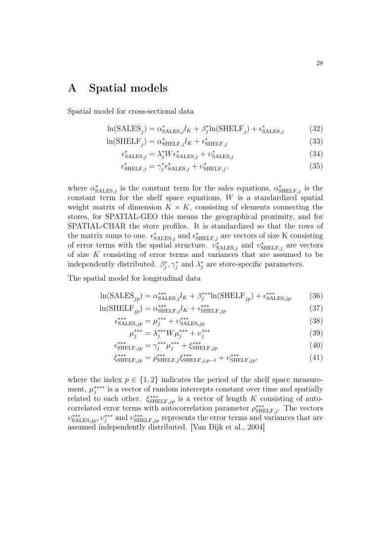
The second approach was to use two different spatial models, which accountsthe endogeneity of space elasticity with spatial structure based on store pro-files (SPATIAL-CHAR model) or based on geographical distance betweenthe stores (SPATIAL-GEO model). The spatial models are presented inAppendix A.

In the case of longitudinal time variation, Van Dijk et al. presents threedifferent approaches. Fixed effect (FE) model and, similar to the cross-sectional data, two different spatial models that are presented in appendixA. (SPATTEMP-GEO and SPATTEMP-CHAR) The fixed effect model addsa store-specific parameter to OLS model with which the endogeneity is at-tempted to be captured. The model is defined as

ln(SALESjp) = µj + βjln(SHELFjp) + τjp + εjp, (8)

where µj a vector representing the store intercepts τjp is a vector of lengthK consisting of the period effects for brand j in period p ∈ {1, 2}.

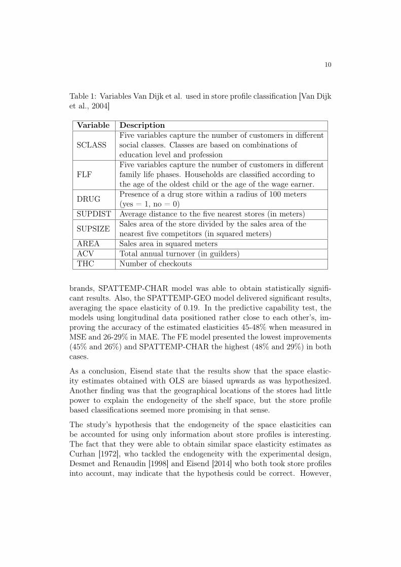
The store profiles used in all spatial models are based on eight variables, asillustrated in Table 1. With the models and data described above, Van Dijket al. estimated and validated the space elasticities for the 5 different brandsof shampoo. As a result for the purely cross-sectional data, they found outthat the elasticities obtained with the basic OLS model were systematicallyhigher (average 0.85) than the ones estimated with other models, for ex-ample SPATIAL-CHAR, giving estimates averaging with space elasticity of0.21, which matches the average of the experiment conducted by Curhan[1972]. The OLSC model positioned between the spatial and OLS mod-els. However, none of the estimates obtained with the SPATIAL-CHAR orSPATIAL-GEO model were statistically significant. When the predictive ca-pabilities of the cross-sectional data were tested with the third shelf spacemeasure point, the SPATIAL-CHAR model was found to be the best, ob-taining 44% more accurate estimates than OLS model, when the accuracymeasured with MSE (Mean Squared Error), and 27% better when measuredwith MAE (Mean Absolute Error). In the case of longitudinal data, similarresults were obtained. Both the FE and SPATTEMP-CHAR models yieldedaverage space elasticities of 0.22. However, in this case for 3 out of five

10

Table 1: Variables Van Dijk et al. used in store profile classification [Van Dijket al., 2004]

Variable Description

SCLASSFive variables capture the number of customers in differentsocial classes. Classes are based on combinations ofeducation level and profession

FLFFive variables capture the number of customers in differentfamily life phases. Households are classified according tothe age of the oldest child or the age of the wage earner.

DRUG Presence of a drug store within a radius of 100 meters(yes = 1, no = 0)

SUPDIST Average distance to the five nearest stores (in meters)

SUPSIZE Sales area of the store divided by the sales area of thenearest five competitors (in squared meters)

AREA Sales area in squared metersACV Total annual turnover (in guilders)THC Number of checkouts

brands, SPATTEMP-CHAR model was able to obtain statistically signifi-cant results. Also, the SPATTEMP-GEO model delivered significant results,averaging the space elasticity of 0.19. In the predictive capability test, themodels using longitudinal data positioned rather close to each other’s, im-proving the accuracy of the estimated elasticities 45-48% when measured inMSE and 26-29% in MAE. The FE model presented the lowest improvements(45% and 26%) and SPATTEMP-CHAR the highest (48% and 29%) in bothcases.

As a conclusion, Eisend state that the results show that the space elastic-ity estimates obtained with OLS are biased upwards as was hypothesized.Another finding was that the geographical locations of the stores had littlepower to explain the endogeneity of the shelf space, but the store profilebased classifications seemed more promising in that sense.

The study’s hypothesis that the endogeneity of the space elasticities canbe accounted for using only information about store profiles is interesting.The fact that they were able to obtain similar space elasticity estimates asCurhan [1972], who tackled the endogeneity with the experimental design,Desmet and Renaudin [1998] and Eisend [2014] who both took store profilesinto account, may indicate that the hypothesis could be correct. However,

11

the spatial models they used were complex, and the results obtained werenot conclusive in every case. A better approach could be to recognize thesources of variations unrelated to shelf space more specifically and controlthose with more case-specific variables than store profiles. These variablescould be related to price, promotion or season and using them in a regressionmodel could result in more accurate estimates with less complicated mod-els. The scope of the study was rather limited, focusing only on differentshampoo brands, so any generalized findings or conclusions cannot be drawnconclusively, but it can be noted that there most likely are many other fac-tors contributing to demand of a product that should be controlled whenestimating the effect of shelf space.

2.3 Effect of the position of product

Dreze et al. [1994] conducted a study discussing also the effect the position ofthe product has on products’ demand. To study the effects of shelf space andposition of a product, they estimated a log-log model to explain the logarithmof unit sales with variables related to space and location elasticities andcontrol variables. For the location effect, they decided to model the positionof the product in the shelf considering two axes. They modeled the salesdependency to horizontal movement as quadratic and to vertical movementas cubic in order to be able to model the different shelf shapes accurately(i.e the refrigerator wells). The model for the effect of position was thus thefollowing

Position = a4Xijk + a5X2ijk + a6Yijk + a7Y

2ijk + a8Y

3ijk, (9)

where Xijk represents the products distance from the left edge of the shelfmeasured from center of the products facings and Yijk represents the productsdistance from the foot of the shelf measured similarly as the X coordinate.i is a brand, j a store and k a week index. For the space elasticity effect,they used a Gompertz growth model because it follows the similar S-shapethey assumed the space elasticity effect to follow. The model they used forthe space elasticity effect was

Space = a9e−kA, (10)

where A is the shelf space allocated for the product and k is the shelf spaceelasticity coefficient. In order to eliminate the effect of variations in salescaused by other than location and space, they added control variables to themodel. They had dummy variables for each brand and store and a price

12

coefficient to incorporate variation those factors cause on sales. The controlportion of the model was

Control = a0 + a11iBi + a2jSj + a3log(Pijk), (11)

where Bi is a dummy for brand i, j is a dummy for store j, and k is a indexfor week. The complete model to explain the logarithm of sales was of form

log(Uijk) = Control + Position + Space, (12)

where the Uijk is the unit sales of product i if it is allocated j facings of spacein shelf k.

They estimated the model with data from 8 product categories obtained from60 stores for time period of 32 weeks in the middle of which the planograms (avisual presentation of products in the shelf according to which the productsare arranged to the shelves) were changed. All promotional sales were re-moved from the dataset. The R2 of the model ranged from 0.53 to 0.86. Theimportance of independent variables remained consistent across categoriesand the order based on the proportion of variance explained was brand andstore, price and position, and shelf space as the least significant variable. Asfor the position effect, they found that it was statistically significant in everycategory, and best vertical positions were at eye-level. Horizontally, the bestpositions varied across categories and the best positions were either on mid-dle of the shelf or near the edges. They estimated an average increase of 39%in sales if the product was moved from the worst possible vertical positionto the best, and average increase of 15% when moving the product similarlyin horizontal direction. The estimated average was 59% when moving fromworst to best in both directions. For shelf space, they found significant re-lations with sales for all except one category. However, the study found outthat in many categories, most of the products had so much shelf space thatthey end up to the upper flat part of the S-curve, meaning that increasingor decreasing the shelf space would not affect the sales significantly.

The findings in this study are significant since they offer data about the effectsof the products’ position on the shelf. As it may be intuitive, the positionof the product has notable effects on sales, and according to the study, evenmore than the plain shelf space itself. The vertically best position being oneye-level sounds realistic and rather intuitive and, therefore, builds confidencein the credibility of the results. Also, the horizontal results sound believableand the difference in the best position could be explained for example withpositions of the shelfs in the store, or some other factors. Based on the resultsof this study, it seems important to account for the position of the product

13

when estimating the effects of shelf space allocation. Dreze et al. estimatedpercentages to demonstrate the benefits of good positioning of products andthe increases in demand seemed very high. However, it must be noted that,as they were estimated for a case where the product is moved from the worstposition to the best, the presented increases can be considered only as upperbounds for the benefit. Because of this, no further conclusions can be drawnfrom them. Furthermore, since this was a single study with a very limitedscope, more research on this subject is needed before the findings can be seenas conclusive.

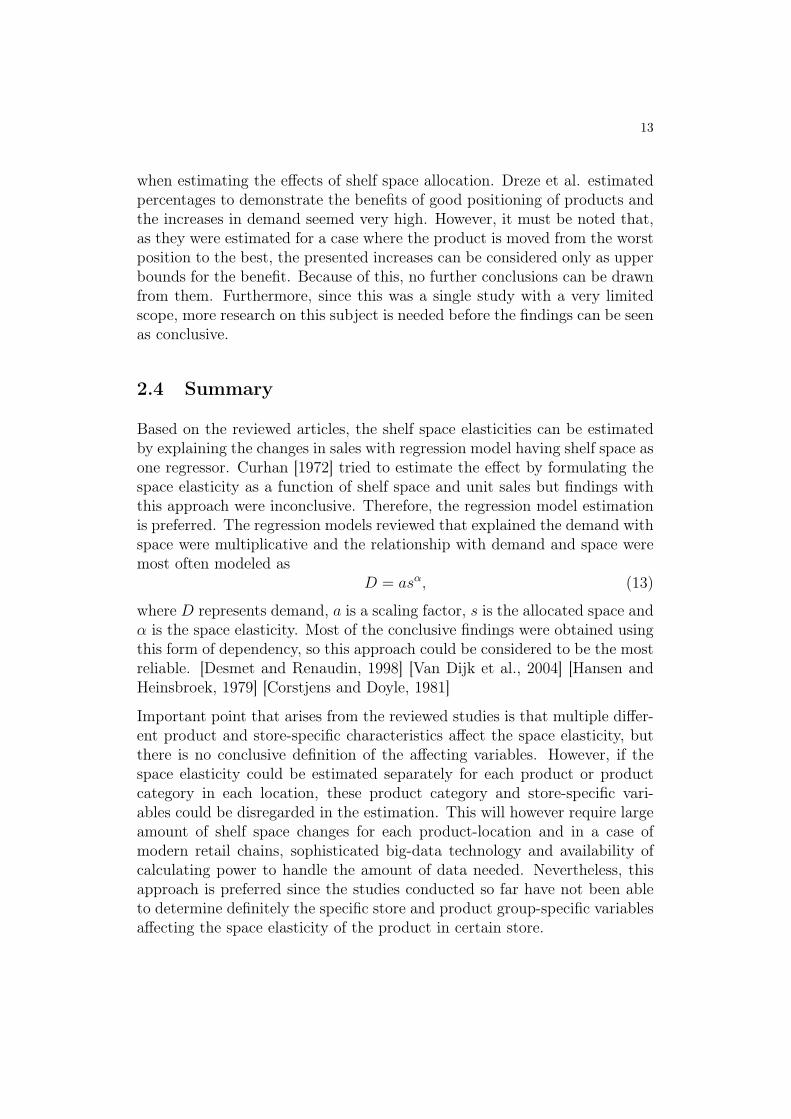
2.4 Summary

Based on the reviewed articles, the shelf space elasticities can be estimatedby explaining the changes in sales with regression model having shelf space asone regressor. Curhan [1972] tried to estimate the effect by formulating thespace elasticity as a function of shelf space and unit sales but findings withthis approach were inconclusive. Therefore, the regression model estimationis preferred. The regression models reviewed that explained the demand withspace were multiplicative and the relationship with demand and space weremost often modeled as

D = asα, (13)

where D represents demand, a is a scaling factor, s is the allocated space andα is the space elasticity. Most of the conclusive findings were obtained usingthis form of dependency, so this approach could be considered to be the mostreliable. [Desmet and Renaudin, 1998] [Van Dijk et al., 2004] [Hansen andHeinsbroek, 1979] [Corstjens and Doyle, 1981]

Important point that arises from the reviewed studies is that multiple differ-ent product and store-specific characteristics affect the space elasticity, butthere is no conclusive definition of the affecting variables. However, if thespace elasticity could be estimated separately for each product or productcategory in each location, these product category and store-specific vari-ables could be disregarded in the estimation. This will however require largeamount of shelf space changes for each product-location and in a case ofmodern retail chains, sophisticated big-data technology and availability ofcalculating power to handle the amount of data needed. Nevertheless, thisapproach is preferred since the studies conducted so far have not been ableto determine definitely the specific store and product group-specific variablesaffecting the space elasticity of the product in certain store.

14

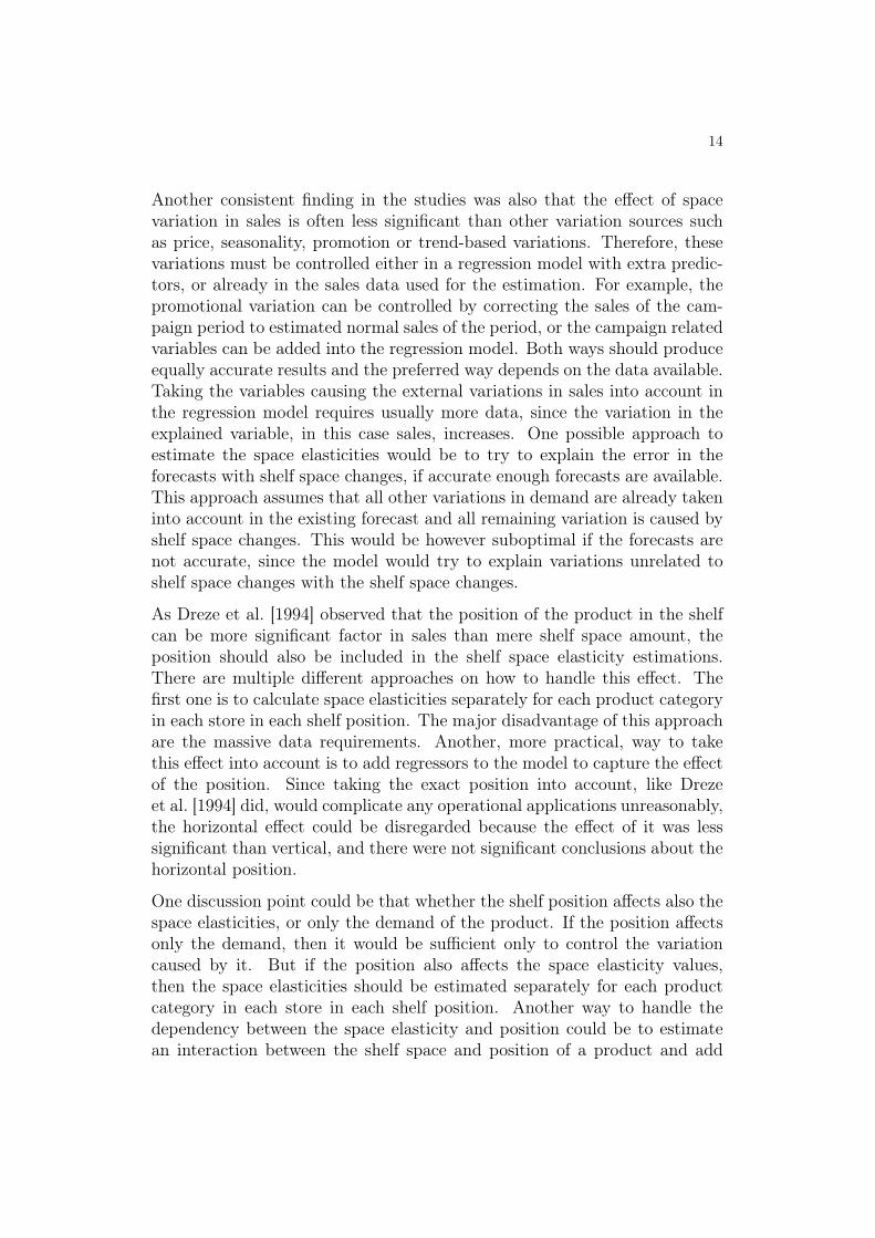
Another consistent finding in the studies was also that the effect of spacevariation in sales is often less significant than other variation sources suchas price, seasonality, promotion or trend-based variations. Therefore, thesevariations must be controlled either in a regression model with extra predic-tors, or already in the sales data used for the estimation. For example, thepromotional variation can be controlled by correcting the sales of the cam-paign period to estimated normal sales of the period, or the campaign relatedvariables can be added into the regression model. Both ways should produceequally accurate results and the preferred way depends on the data available.Taking the variables causing the external variations in sales into account inthe regression model requires usually more data, since the variation in theexplained variable, in this case sales, increases. One possible approach toestimate the space elasticities would be to try to explain the error in theforecasts with shelf space changes, if accurate enough forecasts are available.This approach assumes that all other variations in demand are already takeninto account in the existing forecast and all remaining variation is caused byshelf space changes. This would be however suboptimal if the forecasts arenot accurate, since the model would try to explain variations unrelated toshelf space changes with the shelf space changes.

As Dreze et al. [1994] observed that the position of the product in the shelfcan be more significant factor in sales than mere shelf space amount, theposition should also be included in the shelf space elasticity estimations.There are multiple different approaches on how to handle this effect. Thefirst one is to calculate space elasticities separately for each product categoryin each store in each shelf position. The major disadvantage of this approachare the massive data requirements. Another, more practical, way to takethis effect into account is to add regressors to the model to capture the effectof the position. Since taking the exact position into account, like Drezeet al. [1994] did, would complicate any operational applications unreasonably,the horizontal effect could be disregarded because the effect of it was lesssignificant than vertical, and there were not significant conclusions about thehorizontal position.

One discussion point could be that whether the shelf position affects also thespace elasticities, or only the demand of the product. If the position affectsonly the demand, then it would be sufficient only to control the variationcaused by it. But if the position also affects the space elasticity values,then the space elasticities should be estimated separately for each productcategory in each store in each shelf position. Another way to handle thedependency between the space elasticity and position could be to estimatean interaction between the shelf space and position of a product and add

15

that to the model.

3 Using space elasticity information

3.1 Existing optimization models

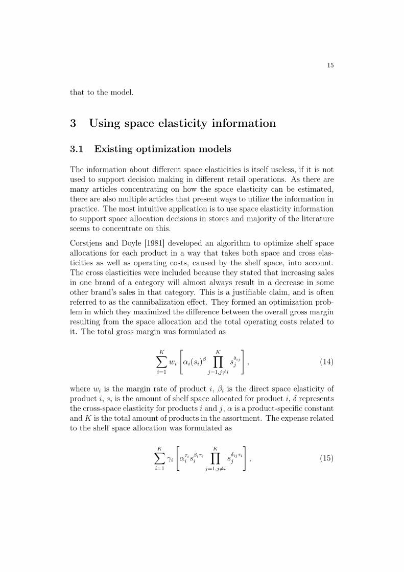
The information about different space elasticities is itself useless, if it is notused to support decision making in different retail operations. As there aremany articles concentrating on how the space elasticity can be estimated,there are also multiple articles that present ways to utilize the information inpractice. The most intuitive application is to use space elasticity informationto support space allocation decisions in stores and majority of the literatureseems to concentrate on this.

Corstjens and Doyle [1981] developed an algorithm to optimize shelf spaceallocations for each product in a way that takes both space and cross elas-ticities as well as operating costs, caused by the shelf space, into account.The cross elasticities were included because they stated that increasing salesin one brand of a category will almost always result in a decrease in someother brand’s sales in that category. This is a justifiable claim, and is oftenreferred to as the cannibalization effect. They formed an optimization prob-lem in which they maximized the difference between the overall gross marginresulting from the space allocation and the total operating costs related toit. The total gross margin was formulated as

K∑i=1

wi

[αi(si)

β

K∏j=1,j 6=i

sδijj

], (14)

where wi is the margin rate of product i, βi is the direct space elasticity ofproduct i, si is the amount of shelf space allocated for product i, δ representsthe cross-space elasticity for products i and j, α is a product-specific constantandK is the total amount of products in the assortment. The expense relatedto the shelf space allocation was formulated as

K∑i=1

γi

[ατii s

βiτii

K∏j=1,j 6=i

sδijτij

], (15)

16

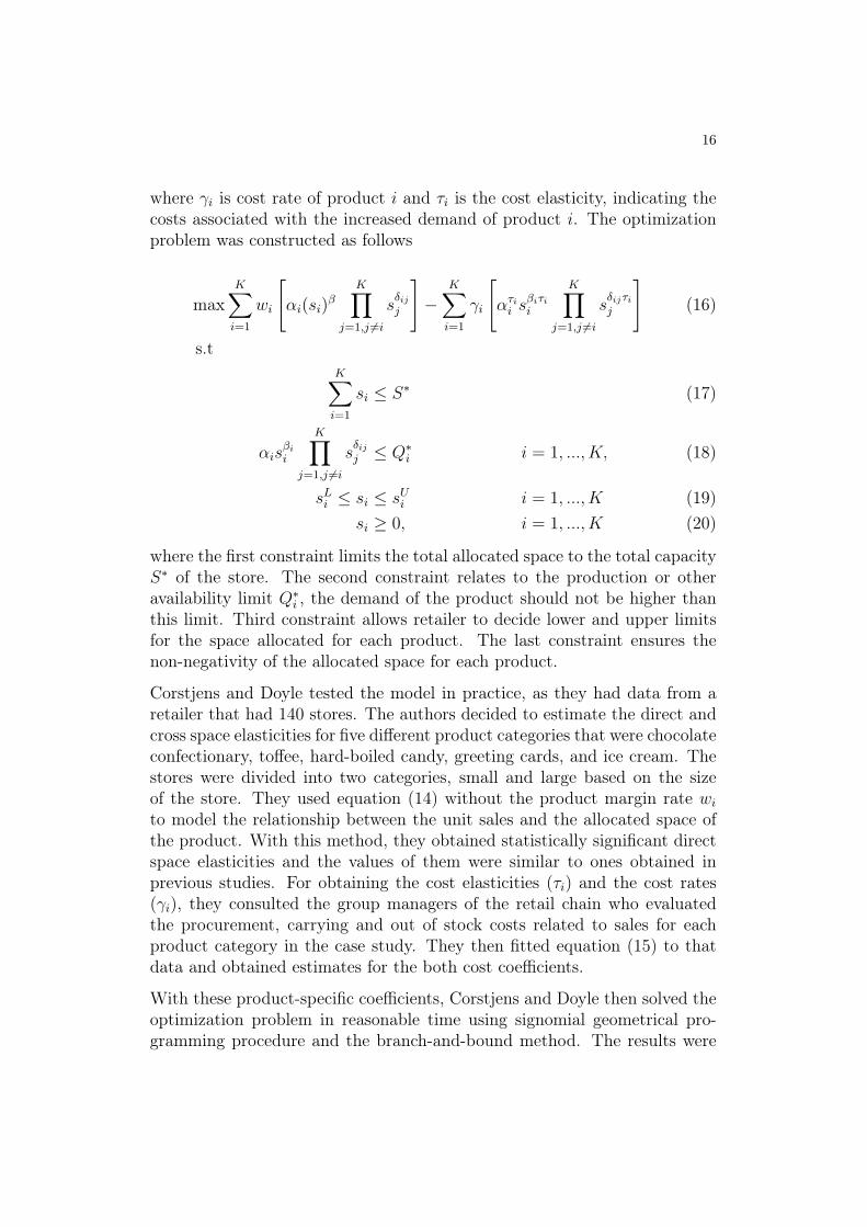
where γi is cost rate of product i and τi is the cost elasticity, indicating thecosts associated with the increased demand of product i. The optimizationproblem was constructed as follows

maxK∑i=1

wi

[αi(si)

β

K∏j=1,j 6=i

sδijj

]−

K∑i=1

γi

[ατii s

βiτii

K∏j=1,j 6=i

sδijτij

](16)

s.tK∑i=1

si ≤ S∗ (17)

αisβii

K∏j=1,j 6=i

sδijj ≤ Q∗i i = 1, ..., K, (18)

sLi ≤ si ≤ sUi i = 1, ..., K (19)si ≥ 0, i = 1, ..., K (20)

where the first constraint limits the total allocated space to the total capacityS∗ of the store. The second constraint relates to the production or otheravailability limit Q∗i , the demand of the product should not be higher thanthis limit. Third constraint allows retailer to decide lower and upper limitsfor the space allocated for each product. The last constraint ensures thenon-negativity of the allocated space for each product.

Corstjens and Doyle tested the model in practice, as they had data from aretailer that had 140 stores. The authors decided to estimate the direct andcross space elasticities for five different product categories that were chocolateconfectionary, toffee, hard-boiled candy, greeting cards, and ice cream. Thestores were divided into two categories, small and large based on the sizeof the store. They used equation (14) without the product margin rate wito model the relationship between the unit sales and the allocated space ofthe product. With this method, they obtained statistically significant directspace elasticities and the values of them were similar to ones obtained inprevious studies. For obtaining the cost elasticities (τi) and the cost rates(γi), they consulted the group managers of the retail chain who evaluatedthe procurement, carrying and out of stock costs related to sales for eachproduct category in the case study. They then fitted equation (15) to thatdata and obtained estimates for the both cost coefficients.

With these product-specific coefficients, Corstjens and Doyle then solved theoptimization problem in reasonable time using signomial geometrical pro-gramming procedure and the branch-and-bound method. The results were

17

reasonable in a practical sense and differed significantly from the existing al-locations, which indicates that significant increases in profit can be achievedby optimizing the allocation. They also state that the profit increases weresubstantial when the allocation patterns were adapted in stores. In order tostudy the effect of the cross elasticities, the authors also estimated the di-rect space elasticities without the cross-effect terms and evaluated the modelwith the new direct space elasticities. They found that the allocation re-sult differed significantly from the previous result and the proposed profitincreases were smaller. Therefore, they concluded that the cross elasticitieshad a significant effect in the model.

Hansen and Heinsbroek [1979] proposed a similar model to use space elastic-ity information, but without the effects of cross elasticities. They modeledthe profit of product i with a formula

πi = miAirαii − ciri, (21)

where mi represents the gross margin of a product i, ri is the space allocatedfor product i, Ai is a scale factor, αi denotes the space elasticity and ci is theunit cost of space. They formulated an optimization problem

maxn∑i=1

πi − f(N,L) (22)

s.tn∑i=1

ri ≤ R (23)

ri ≥ rmi yi, i = 1, 2, ..., n (24)ri ≤ Ryi, i = 1, 2, ..., n (25)yi ∈ {0, 1}, i = 1, 2, ..., n (26)rili∈ N+, i = 1, 2, ..., n (27)

where f(N,L) is a function of a replenishment frequency N (times per week)and the lead time L (days), when L = 0, there is backroom stock for theproduct and the shelf can be replenished from the backroom, when L > 0,backroom stock is not available and it will take L days for the new stock toget to the store. Term li represents the length of one facing of product i, yiis a boolean variable and is 1 when the product is part of the assortment and0, otherwise; rmi is the minimum amount of space to be allocated for prod-uct i, if it is a part of assortment and R is a total shelf space of the store.

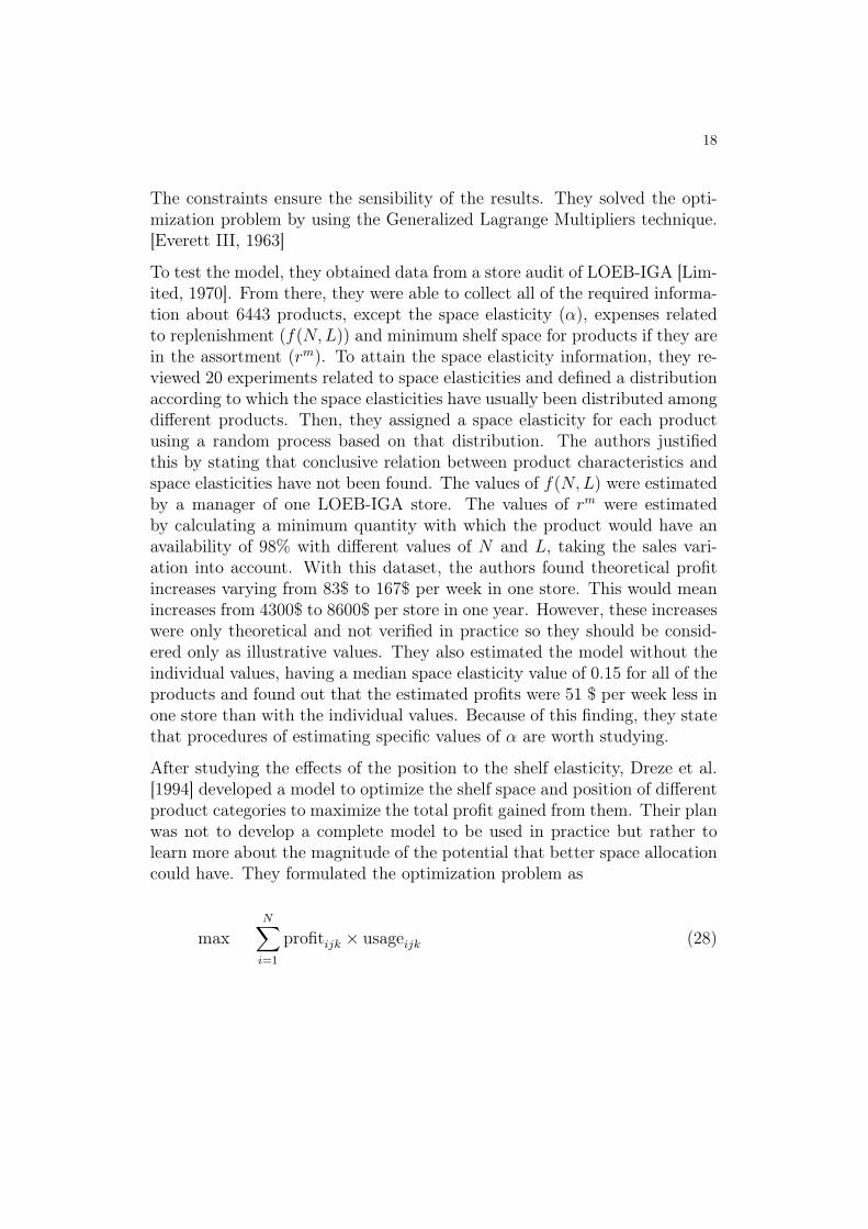
18

The constraints ensure the sensibility of the results. They solved the opti-mization problem by using the Generalized Lagrange Multipliers technique.[Everett III, 1963]

To test the model, they obtained data from a store audit of LOEB-IGA [Lim-ited, 1970]. From there, they were able to collect all of the required informa-tion about 6443 products, except the space elasticity (α), expenses relatedto replenishment (f(N,L)) and minimum shelf space for products if they arein the assortment (rm). To attain the space elasticity information, they re-viewed 20 experiments related to space elasticities and defined a distributionaccording to which the space elasticities have usually been distributed amongdifferent products. Then, they assigned a space elasticity for each productusing a random process based on that distribution. The authors justifiedthis by stating that conclusive relation between product characteristics andspace elasticities have not been found. The values of f(N,L) were estimatedby a manager of one LOEB-IGA store. The values of rm were estimatedby calculating a minimum quantity with which the product would have anavailability of 98% with different values of N and L, taking the sales vari-ation into account. With this dataset, the authors found theoretical profitincreases varying from 83$ to 167$ per week in one store. This would meanincreases from 4300$ to 8600$ per store in one year. However, these increaseswere only theoretical and not verified in practice so they should be consid-ered only as illustrative values. They also estimated the model without theindividual values, having a median space elasticity value of 0.15 for all of theproducts and found out that the estimated profits were 51 $ per week less inone store than with the individual values. Because of this finding, they statethat procedures of estimating specific values of α are worth studying.

After studying the effects of the position to the shelf elasticity, Dreze et al.[1994] developed a model to optimize the shelf space and position of differentproduct categories to maximize the total profit gained from them. Their planwas not to develop a complete model to be used in practice but rather tolearn more about the magnitude of the potential that better space allocationcould have. They formulated the optimization problem as

maxN∑i=1

profitijk × usageijk (28)

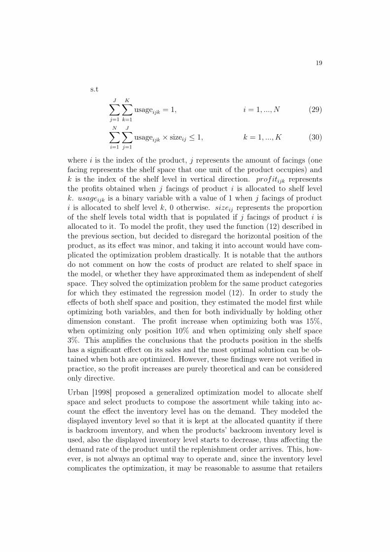
19

s.tJ∑j=1

K∑k=1

usageijk = 1, i = 1, ..., N (29)

N∑i=1

J∑j=1

usageijk × sizeij ≤ 1, k = 1, ..., K (30)

where i is the index of the product, j represents the amount of facings (onefacing represents the shelf space that one unit of the product occupies) andk is the index of the shelf level in vertical direction. profitijk representsthe profits obtained when j facings of product i is allocated to shelf levelk. usageijk is a binary variable with a value of 1 when j facings of producti is allocated to shelf level k, 0 otherwise. sizeij represents the proportionof the shelf levels total width that is populated if j facings of product i isallocated to it. To model the profit, they used the function (12) described inthe previous section, but decided to disregard the horizontal position of theproduct, as its effect was minor, and taking it into account would have com-plicated the optimization problem drastically. It is notable that the authorsdo not comment on how the costs of product are related to shelf space inthe model, or whether they have approximated them as independent of shelfspace. They solved the optimization problem for the same product categoriesfor which they estimated the regression model (12). In order to study theeffects of both shelf space and position, they estimated the model first whileoptimizing both variables, and then for both individually by holding otherdimension constant. The profit increase when optimizing both was 15%,when optimizing only position 10% and when optimizing only shelf space3%. This amplifies the conclusions that the products position in the shelfshas a significant effect on its sales and the most optimal solution can be ob-tained when both are optimized. However, these findings were not verified inpractice, so the profit increases are purely theoretical and can be consideredonly directive.

Urban [1998] proposed a generalized optimization model to allocate shelfspace and select products to compose the assortment while taking into ac-count the effect the inventory level has on the demand. They modeled thedisplayed inventory level so that it is kept at the allocated quantity if thereis backroom inventory, and when the products’ backroom inventory level isused, also the displayed inventory level starts to decrease, thus affecting thedemand rate of the product until the replenishment order arrives. This, how-ever, is not always an optimal way to operate and, since the inventory levelcomplicates the optimization, it may be reasonable to assume that retailers

20

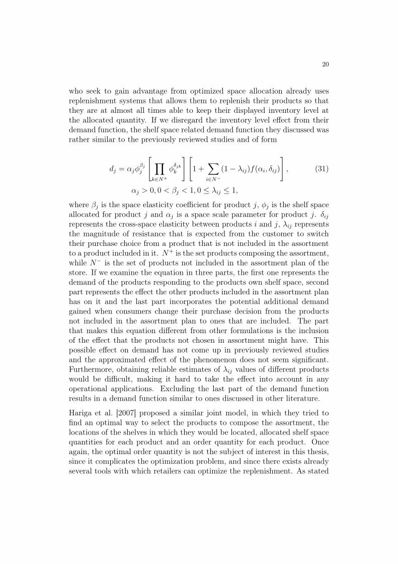
who seek to gain advantage from optimized space allocation already usesreplenishment systems that allows them to replenish their products so thatthey are at almost all times able to keep their displayed inventory level atthe allocated quantity. If we disregard the inventory level effect from theirdemand function, the shelf space related demand function they discussed wasrather similar to the previously reviewed studies and of form

dj = αjφβjj

[ ∏k∈N+

φδjkk

][1 +

∑i∈N−

(1− λij)f(αi, δij)

], (31)

αj > 0, 0 < βj < 1, 0 ≤ λij ≤ 1,

where βj is the space elasticity coefficient for product j, φj is the shelf spaceallocated for product j and αj is a space scale parameter for product j. δijrepresents the cross-space elasticity between products i and j, λij representsthe magnitude of resistance that is expected from the customer to switchtheir purchase choice from a product that is not included in the assortmentto a product included in it. N+ is the set products composing the assortment,while N− is the set of products not included in the assortment plan of thestore. If we examine the equation in three parts, the first one represents thedemand of the products responding to the products own shelf space, secondpart represents the effect the other products included in the assortment planhas on it and the last part incorporates the potential additional demandgained when consumers change their purchase decision from the productsnot included in the assortment plan to ones that are included. The partthat makes this equation different from other formulations is the inclusionof the effect that the products not chosen in assortment might have. Thispossible effect on demand has not come up in previously reviewed studiesand the approximated effect of the phenomenon does not seem significant.Furthermore, obtaining reliable estimates of λij values of different productswould be difficult, making it hard to take the effect into account in anyoperational applications. Excluding the last part of the demand functionresults in a demand function similar to ones discussed in other literature.

Hariga et al. [2007] proposed a similar joint model, in which they tried tofind an optimal way to select the products to compose the assortment, thelocations of the shelves in which they would be located, allocated shelf spacequantities for each product and an order quantity for each product. Onceagain, the optimal order quantity is not the subject of interest in this thesis,since it complicates the optimization problem, and since there exists alreadyseveral tools with which retailers can optimize the replenishment. As stated

21

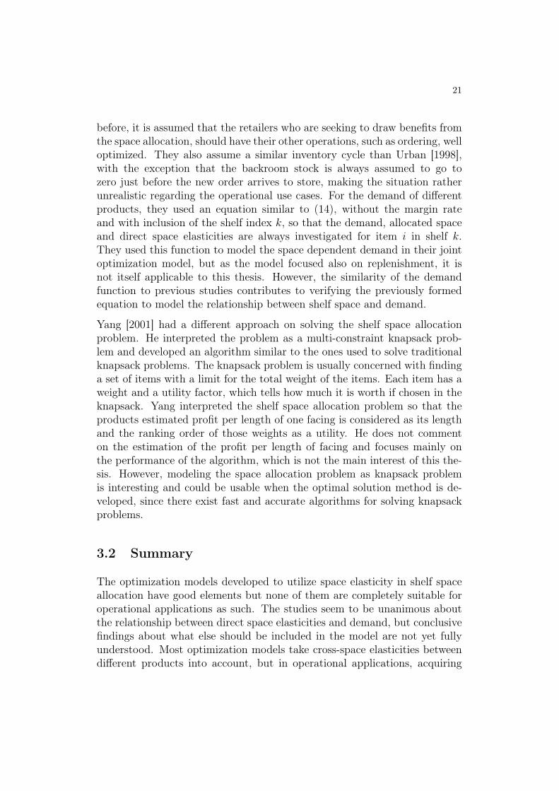
before, it is assumed that the retailers who are seeking to draw benefits fromthe space allocation, should have their other operations, such as ordering, welloptimized. They also assume a similar inventory cycle than Urban [1998],with the exception that the backroom stock is always assumed to go tozero just before the new order arrives to store, making the situation ratherunrealistic regarding the operational use cases. For the demand of differentproducts, they used an equation similar to (14), without the margin rateand with inclusion of the shelf index k, so that the demand, allocated spaceand direct space elasticities are always investigated for item i in shelf k.They used this function to model the space dependent demand in their jointoptimization model, but as the model focused also on replenishment, it isnot itself applicable to this thesis. However, the similarity of the demandfunction to previous studies contributes to verifying the previously formedequation to model the relationship between shelf space and demand.

Yang [2001] had a different approach on solving the shelf space allocationproblem. He interpreted the problem as a multi-constraint knapsack prob-lem and developed an algorithm similar to the ones used to solve traditionalknapsack problems. The knapsack problem is usually concerned with findinga set of items with a limit for the total weight of the items. Each item has aweight and a utility factor, which tells how much it is worth if chosen in theknapsack. Yang interpreted the shelf space allocation problem so that theproducts estimated profit per length of one facing is considered as its lengthand the ranking order of those weights as a utility. He does not commenton the estimation of the profit per length of facing and focuses mainly onthe performance of the algorithm, which is not the main interest of this the-sis. However, modeling the space allocation problem as knapsack problemis interesting and could be usable when the optimal solution method is de-veloped, since there exist fast and accurate algorithms for solving knapsackproblems.

3.2 Summary

The optimization models developed to utilize space elasticity in shelf spaceallocation have good elements but none of them are completely suitable foroperational applications as such. The studies seem to be unanimous aboutthe relationship between direct space elasticities and demand, but conclusivefindings about what else should be included in the model are not yet fullyunderstood. Most optimization models take cross-space elasticities betweendifferent products into account, but in operational applications, acquiring

22

reliable information about the relationship between products is both difficultand time consuming. The cannibalization effect is much stronger when theshelf space effect is studied for each product individually, since consumerscan easily substitute one brand with another from the same category, but ifthey are estimated only for each product category, the effect of cross spaceelasticities depreciate. The effect of cross elasticities can thus be minimizedby evaluating the space elasticities only for each product category, and opti-mizing the space allocation on product category level. This approach shouldjustify the exclusion of the effect of cross elasticities, thus making it easierto obtain the data needed in continuous operational application.

As discussed in the previous section, the position of the product in the shelfplays an important role in the relationship between shelf space allocation anddemand. This effect, therefore, needs to be taken into account for the opti-mization model to deliver actually beneficial results. The remaining questionis how to take the effect of space into account in the optimization models.One approach could be to divide the shelf in different blocks and value theshelf space in them differently. The optimization model could then allo-cate the shelf space separately for each block, similarly to approach of Drezeet al. [1994] in equation (28). However, this will complicate the optimiza-tion model, since the amount allocated to each block needs to be handledseparately. Another approach is to include the position to the problem asanother decision variable. Since taking the exact position into account wouldresult in a really complex set of possible solutions, the space measure shouldbe simplified somehow, for example by dividing the shelf into blocks.

Many of the papers also used profit functions that included shelf space re-lated costs for each product in the assortment. The assumption that theshelving and other shelf space related costs are different for each product isvalid and could result for example from different sales packages. Regardingthe operational applications, the information required to estimate the dif-ferent costs reliably for each product is hard, since it can rarely be derivedfrom data. Obtaining the data would therefore require interviewing the storemanagers, and the estimates could still be inaccurate. In operational appli-cations, it would be desirable to be able to draw all necessary informationfrom available data, so taking these different costs into account would com-plicate the application substantially. However, when the space allocation isoptimized on a product category level, the different space allocation relatedcosts of products could be equalized, so that the costs between product cat-egories could be estimated as constant. However, this should be validated infuture studies. If the costs could be estimated as constant for all categories,the space related costs could be disregarded from the optimization problem

23

and the function to be maximized could be the demand related profit of allproduct categories.

Regardless of being the most intuitive option, optimizing the shelf spaceallocation is not the only way to use shelf space elasticity information inoperational applications. Together with information about price elasticities,space elasticity could be utilized in promotion planning. For example, a de-mand of a product or product category that has a high space elasticity andlow price elasticity benefits more from promotions that focuses on the place-ment of the products rather than large discounts. This way the retailer wouldobtain a higher return from the promotions, as they would be able to holdup a higher profit margin. Similarly, by using higher discount percent withless shelf space for products/product categories that have high price elastic-ity maximizes the demand of the product while saving more and better shelfspace to products that benefit more from it. However, determining the ex-act methods on how to operationalize this information reliably in promotionplanning requires more information about the subject and should thereforebe a subject of further studies. Another possible approach for retailers onexploiting the space elasticity would be to use it in discussions with the man-ufacturers and importers. Manufacturers often negotiate deals with retailersto ensure sufficient amount of shelf space for their products, by selling theirproducts with smaller margins if the retailers agree to allocate more shelfspace to it. However, if retailers have accurate information about how theproducts demand depends on its shelf space, they are able to price their shelfspace more effectively. Similarly, operationalizing this strategy requires moreresearch on the subject.

4 Conclusions

This thesis conducted a literature review about the studies discussing theestimation and usage of space elasticity information. Based on the review,we constructed guidelines to generalize and operationalize the estimation andutilization of the space elasticity information.

It can be concluded from the reviewed articles that a significant relation-ship between shelf space and demand exists and the magnitude of it variesacross product categories and stores. The space elasticity coefficient averagessomewhere below 0.2, according to most recent studies. The value of spaceelasticity of a product is affected by multiple variables related to its cate-gory and store it is sold in, but the studies have not been able to determine

24

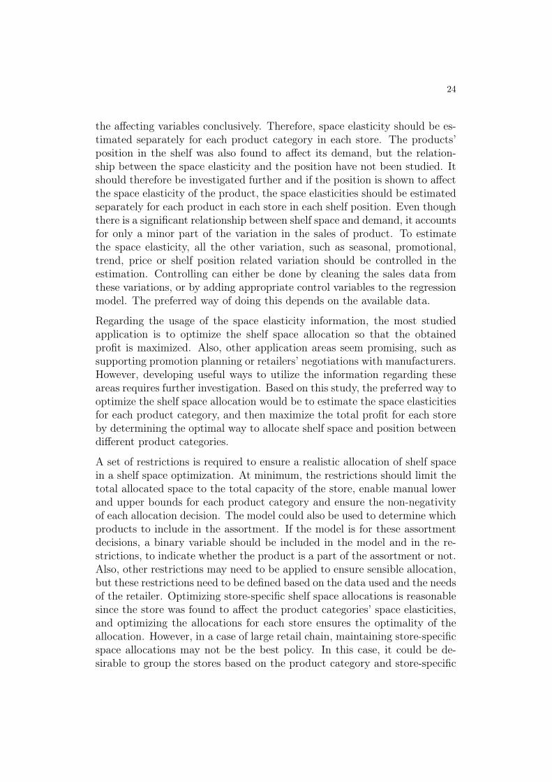
the affecting variables conclusively. Therefore, space elasticity should be es-timated separately for each product category in each store. The products’position in the shelf was also found to affect its demand, but the relation-ship between the space elasticity and the position have not been studied. Itshould therefore be investigated further and if the position is shown to affectthe space elasticity of the product, the space elasticities should be estimatedseparately for each product in each store in each shelf position. Even thoughthere is a significant relationship between shelf space and demand, it accountsfor only a minor part of the variation in the sales of product. To estimatethe space elasticity, all the other variation, such as seasonal, promotional,trend, price or shelf position related variation should be controlled in theestimation. Controlling can either be done by cleaning the sales data fromthese variations, or by adding appropriate control variables to the regressionmodel. The preferred way of doing this depends on the available data.

Regarding the usage of the space elasticity information, the most studiedapplication is to optimize the shelf space allocation so that the obtainedprofit is maximized. Also, other application areas seem promising, such assupporting promotion planning or retailers’ negotiations with manufacturers.However, developing useful ways to utilize the information regarding theseareas requires further investigation. Based on this study, the preferred way tooptimize the shelf space allocation would be to estimate the space elasticitiesfor each product category, and then maximize the total profit for each storeby determining the optimal way to allocate shelf space and position betweendifferent product categories.

A set of restrictions is required to ensure a realistic allocation of shelf spacein a shelf space optimization. At minimum, the restrictions should limit thetotal allocated space to the total capacity of the store, enable manual lowerand upper bounds for each product category and ensure the non-negativityof each allocation decision. The model could also be used to determine whichproducts to include in the assortment. If the model is for these assortmentdecisions, a binary variable should be included in the model and in the re-strictions, to indicate whether the product is a part of the assortment or not.Also, other restrictions may need to be applied to ensure sensible allocation,but these restrictions need to be defined based on the data used and the needsof the retailer. Optimizing store-specific shelf space allocations is reasonablesince the store was found to affect the product categories’ space elasticities,and optimizing the allocations for each store ensures the optimality of theallocation. However, in a case of large retail chain, maintaining store-specificspace allocations may not be the best policy. In this case, it could be de-sirable to group the stores based on the product category and store-specific

25

space elasticities and use the average of each category’s space elasticity as arepresentative of each product category in a store group. Then, the alloca-tions could be calculated for each store group, so that only a few differentspace allocations should be maintained at the same retail chain.

26

ReferencesMarcel Corstjens and Peter Doyle. A model for optimizing retail space allo-cations. Management Science, 27(7):822–833, 1981.

Keith Cox. The responsiveness of food sales to shelf space changes in super-markets. Journal of marketing Research, pages 63–67, 1964.

Ronald C Curhan. The relationship between shelf space and unit sales insupermarkets. Journal of Marketing Research, pages 406–412, 1972.

Pierre Desmet and Valérie Renaudin. Estimation of product category salesresponsiveness to allocated shelf space. International Journal of Researchin Marketing, 15(5):443–457, 1998.

Xavier Dreze, Stephen J Hoch, and Mary E Purk. Shelf management andspace elasticity. Journal of Retailing, 70(4):301–326, 1994.

Martin Eisend. Shelf space elasticity: A meta-analysis. Journal of Retailing,90(2):168–181, 2014.

Hugh Everett III. Generalized lagrange multiplier method for solving prob-lems of optimum allocation of resources. Operations research, 11(3):399–417, 1963.

Pierre Hansen and Hans Heinsbroek. Product selection and space allocationin supermarkets. European journal of operational research, 3(6):474–484,1979.

Moncer A Hariga, Abdulrahman Al-Ahmari, and Abdel-Rahman A Mo-hamed. A joint optimisation model for inventory replenishment, productassortment, shelf space and display area allocation decisions. EuropeanJournal of Operational Research, 181(1):239–251, 2007.

M. Loeb Limited. Supermarket Methods Presents the LOEB-IGA Study:A Profile of Product Performance : a Study of Gross Profits by the Ed-itors. LOEB-IGA, 1970. URL https://books.google.fi/books?id=KScAtAEACAAJ.

Timothy L Urban. An inventory-theoretic approach to product assortmentand shelf-space allocation. Journal of Retailing, 74(1):15–35, 1998.

Albert Van Dijk, Harald J Van Heerde, Peter SH Leeflang, and Dick R Wit-tink. Similarity-based spatial methods to estimate shelf space elasticities.Quantitative Marketing and Economics, 2(3):257–277, 2004.

27

Ming-Hsien Yang. An efficient algorithm to allocate shelf space. Europeanjournal of operational research, 131(1):107–118, 2001.

28

A Spatial models

Spatial model for cross-sectional data

ln(SALESj) = α∗SALES,jlK + β∗j ln(SHELFj) + ε∗SALES,j (32)

ln(SHELFj) = α∗SHELF,jlK + ε∗SHELF,j (33)

ε∗SALES,j = λ∗jWε∗SALES,j + υ∗SALES,j (34)ε∗SHELF,j = γ∗j ε

∗SALES,j + υ∗SHELF,j, (35)

where α∗SALES,j is the constant term for the sales equations, α∗SHELF,j is theconstant term for the shelf space equations, W is a standardized spatialweight matrix of dimension K × K, consisting of elements connecting thestores, for SPATIAL-GEO this means the geographical proximity, and forSPATIAL-CHAR the store profiles. It is standardized so that the rows ofthe matrix sums to one. ε∗SALES,j and ε∗SHELF,j are vectors of size K consistingof error terms with the spatial structure. υ∗SALES,j and υ∗SHELF,j are vectorsof size K consisting of error terms and variances that are assumed to beindependently distributed. β∗j , γ∗j and λ∗j are store-specific parameters.

The spatial model for longitudinal data

ln(SALESjp) = α∗∗∗SALES,jlK + β∗∗∗j ln(SHELFjp) + ε∗∗∗SALES,jp (36)

ln(SHELFjp) = α∗∗∗SHELF,jlK + ε∗∗∗SHELF,jp (37)

ε∗∗∗SALES,jp = µ∗∗∗j + υ∗∗∗SALES,jp (38)µ∗∗∗j = λ∗∗∗j Wµ∗∗∗j + υ∗∗∗j (39)

ε∗∗∗SHELF,jp = γ∗∗∗j µ∗∗∗j + ξ∗∗∗SHELF,jp (40)ξ∗∗∗SHELF,jp = ρ∗∗∗SHELF,jξ

∗∗∗SHELF,j,p−1 + υ∗∗∗SHELF,jp, (41)

where the index p ∈ {1, 2} indicates the period of the shelf space measure-ment, µ∗∗∗∗j is a vector of random intercepts constant over time and spatiallyrelated to each other. ξ∗∗∗SHELF,jp is a vector of length K consisting of auto-correlated error terms with autocorrelation parameter ρ∗∗∗SHELF,j. The vectorsυ∗∗∗SALES,jp, υ

∗∗∗j and υ∗∗∗SHELF,jp represents the error terms and variances that are

assumed independently distributed. [Van Dijk et al., 2004]