Modeling Stress Strain Relationships and Predicting

Failure Probabilities For Graphite Core Components

Reactor Concepts RD&D Dr. Stephen Duffy

Cleveland State University

Brian Robinson, Federal POC Robert Bratton, Technical POC

Project No. 09-838

CLOSE OUT REPORT

Project Title: 09-347: Modeling Stress Strain Relationships and Predicting Failure Probabilities For Graphite Core Components

Covering Period: October 1, 2009 through September 30, 2012

Date of Report: September 9, 2013

Recipient: Cleveland State University

Address: Civil & Environmental Engineering Department 2121 Euclid Avenue, SH 114 Cleveland, Ohio 44115-2214

Contract Number: 00088589 Project Number: 09-347

Principal Investigator: Stephen F Duffy 216-687-3874 (office), 330-388-0511 (cell) s.duffy@csuohio.edu

Collaborators: no other collaborators

1

I. Introduction

Despite current events associated with the light water reactors in Fukishima, Japan, energy producers continue to look at nuclear power as a viable alternative for power generation. There are several new designs that transcend the older light water reactors that failed to perform safely in Japan. Among the designs for the next generation power plant is the very high temperature reactors (VHTR), molten salt reactors, and super critical water cooled reactors. In addition to generating electricity the VHTR will be able to produce hydrogen without consuming fossil fuels or emitting greenhouse gasses which is a distinct benefit. Emerging technologies often depend on new materials or the innovative use of existing material, and graphite is a key material in the design of several of the next generation nuclear power plants.

Currently there are two designs for the VHTR. The first design utilizes a prismatic core reactor. The second design is known as a pebble bed reactor. In the prismatic core reactor the nuclear fuel is contained in fuel rods. Hexagonal graphite blocks that hold the fuel rods are used to moderate the nuclear reaction. The cooling gas runs in channels inside the hexagonal prismatic blocks. The reactor is comprised of an array of blocks that accommodate fuel rods, control rods, and cooling channels.

Alternatively, in pebble bed reactors the fissile material, the moderator, and a fission product barrier are contained in softball sized pebbles. The pebbles are continuously cycled through reactor channels and are removed from the bottom of the reactor. The pebbles are then tested to determine how much nuclear fuel remains. If sufficient fuel remains the pebble is returned to the reactor. Process cooling gas flows around the pebbles as they are cycled through the reactor.

Prismatic core reactors are designed to reach higher service temperatures than the pebble bed reactor. The initial designs for the prismatic core reactors call for an outlet temperature ranging from 850 C to 1000 C. At these temperatures water can be “cracked” into hydrogen and oxygen in the presence of a catalyst. Thus a virtuous (i.e., clean) process is established that produces electricity, hydrogen feed stocks for the chemical industry, and pure oxygen.

The core components of the VHTR cannot be fabricated from of metals due to radiation levels and operating temperatures. Graphite has long been utilized as a moderator material. Several countries including the United States, France, the United Kingdom, Germany, South Africa, Japan, and China support evolving technologies for nuclear graphite material systems that focus on several aspects of the behavior of graphite in reactor cores. These technologies are key to the VHTR program.

I.1 Constitutive Models

Accurate stress states are a necessity in designing reactor components. The effort here assumes the stress-strain response for nuclear grade graphite can be characterized using an inelastic constitutive model that accounts for different behavior in tension and compression, as well as accounts for material anisotropy. Graphite has a relatively small elastic range. Moreover, the stress-strain relationship for graphite is for the most part nonlinear. An objective

2

of this project is the development of a comprehensive constitutive model that will predict both elastic and inelastic cyclic phenomenological behavior. An appropriate elasticity model is integrated with the proposed inelastic constitutive model when cyclic loading is discussed. In the presence of time dependent phenomenon such as creep, one needs a viscoplastic constitutive model. The time independent inelastic model presented here can be extended to include rate dependent effects. This is left for future work.

As was just mentioned one of the fundamental behaviors that must be accounted for in graphite materials is the different behaviors in tension and compression. Graphite is not the only material that behaves differently in tension and compression under mechanical loads. Concrete also exhibits different properties in tension and compression, and inelastic constitutive models exists for concrete, e.g., the phenomenological model developed by William and Warnke (1974), Ottosen (1977) and Hsieh et al. (1979). An effort was made to extend the William and Warnke (1974) model for graphite to include material anisotropy. That effort was unsuccessful. An alternative constitutive model proposed by Green and Mkrtichian (1977) was adopted in this effort. Aspects of this model are thoroughly presented and the model is successfully extended to include anisotropy in a unified inelastic model.

Issues such as neutron radiation damage in graphite which initially causes an increase in the modulus of elasticity and then deteriorates with time are one of the many topics under current study that was not be addressed in this project. In the future plans call for modeling this phenomenon by incorporating damage state variables. Current constitutive models for graphite are empirically based account for radiation damage serves as a starting point for this issue.

I.2 Probabilistic Failure Analyses

The nuclear moderator and major structural components for VHTRs are constructed from graphite. During operations the graphite components are subjected to complex stress states arising from structural loads, thermal gradients, neutron irradiation damage, and seismic events, any and/or all of which can lead to failure. As discussed by Burchell, et al (2007) failure theories that predict reliability of graphite components for a given stress state are important.

Graphite is often described as a brittle or quasi-brittle material. Tabeddor (1979) and Vijayakumar, et al (1987, 1990) emphasize the anisotropic effect the elongated grain graphite structure has on the stress-strain relationship for graphite. These authors also discuss the aspect that the material behaves differently in tension and in compression. These two properties, i.e., material anisotropy and different behavior in tension and compression, make formulating a failure model challenging.

Classical brittle material failure criteria can include phenomenological failure criteria, as well as fracture mechanics based models. The approach taken in linear elastic fracture mechanics involves estimating the amount of energy needed to grow a pre-existing crack. The earliest fracture mechanics approach for unstable crack growth was proposed by Griffiths (1921). Li (2001) points out that the strain energy release rate approach has proven to be quite useful for metal alloys. However, linear elastic fracture mechanics is difficult to apply to anisotropic materials with a microstructure that makes it difficult to identify a “critical” flaw. An alternative

3

approach can be found in the numerous phenomenological failure criteria identified in the engineering literature.

Popular phenomenological failure criteria for brittle materials tend to build on the one parameter Tresca model (1864), and the two parameters Mohr-Coulomb failure criterion (1776) that has been utilized for cohesive-frictional solids. Included with these fundamental model is the von Mises criterion (1913) (a one-parameter model) and the two parameter Drucker-Prager failure criterion (1952) for pressure-dependent solids. In the past these models have been used to capture failure due to ductile yielding. Paul (1968) developed a generalized pyramidal criterion model which he proposed for use with brittle material. In Paul’s work, an assumption that the yield criteria surface is piecewise linear is utilized which is similar to Tresca’s model. The Willam and Warnke (1974) model is a three-parameter model that captures different behavior in tension and compression exhibited by concrete. Willam and Warnke’s model is composed of piecewise continuous functions that maintain smooth transitions across the boundaries of the functions. The proposed work here will focus extensively on models similar to Willam and Warnke’s efforts.

With regards to phenomenological models that account for anisotropic behavior the classic Tsai and Wu (1971) failure criterion is a seminal effort. Presented in the context of invariant based stress tensors for fiber-reinforced composites, the Tsai-Wu criterion is widely used in engineering for different types of anisotropic materials. In addition Boehler and Sawczuk (1977), Boehler (1987), as well as Boehler and Kirillov (1994) developed yield criterion utilizing the framework of anisotropic invariant theory. Yield functions can easily serve as the framework for failure models. Subsequent work by Nova and Zaninetti (1990) developed an anisotropic failure criterion for materials with failure behavior different in tension and compression. Theocaris (1991) proposed an elliptic paraboloid failure criterion that accounts for different behavior in tension and compression. An invariant formulation of a failure criterion for transversely isotropic solids was proposed by Cazacu et al. (1998, 1999). Cazacu’s criterion reduces to the Mises-Schleicher criterion (1926), which captured different behavior in tension and compression for isotropic conditions. Green and Mkrtichian (1977) also proposed functional forms account for different behavior in tension and compression. Their work will be focused on later in this effort

In addition to anisotropy and different behavior in tension and compression, failure of components fabricated from graphite is also governed by the scatter in strength. When material strength varies, it is desirable to be able to predict the probability of failure for a component given a stress state. Weibull (1951) first introduced a method for quantifying variability in failure strength and the size effect in brittle material. His approach was based on the weakest link theory. The work by Batdorf and Crose (1974) represented the first attempt at extending fracture mechanics to reliability analysis in a consistent and rational manner. Work by Gyekenyesi (1986), Cooper, et al. (1986, 1988) and Lamon (1990) are representative of the reliability design philosophy used in analyzing structural components fabricated from monolithic ceramic. Duffy et al. (1990a, 1990b, 1991, 1993, 1994) presented an array of failure models to predict reliability of ceramic components that have isotropic, transversely isotropic, or orthotropic material symmetry. For the most part these models were based on developing an appropriate integrity basis for each type of anisotropy.

4

The work in this project assumed the existence of a threshold function, which also served as a inelastic potential function. Since the inelastic potential function is scalar valued, tensorial invariant theory was used to construct appropriate functions. Threshold functions are extended to account for graphites that exhibit transversely isotropic behavior. Specifically an inelastic constitutive model with isotropic threshold functions proposed by Green and Mkrtichian (1977) were initially adopted for this work. Both the isotropic and anisotropic inelastic models are derived based on associated threshold functions. The same functional forms for the inelastic threshold functions were utilized to formulate failure functions. The parameters associated with the failure function are treated as random variables. The result is a probabilistic based failure model that accounts for the unique phenomenological behavior of graphite, i.e., different behavior in tension ad compression as well as anisotropic failure.

I.3 Stress Based Functions and Integrity Bases

A function associated with a phenomenological failure criterion based on multi-axial stress for isotropic materials will have the basic form

ijff (1)

This function is dependent on the Cauchy stress tensor, ij , which is a second order tensor, and parameters associated with material strength. Given a change in reference coordinates, e.g., a rotation of coordinate axes, the components of the stress tensor change. We wish to formulate a scalar valued failure function so that it is not affected when components of the stress tensors change from a simple orthogonal transformation of coordinate axes. A convenient way of formulating a failure function to accomplish this is utilizing the invariants of stress. The development below follows the method outlined by Duffy (1987) and serves as a brief discussion on the invariants that comprise an integrity basis.

Assume f is a scalar valued function dependent upon several second order tensors, i.e.,

CBAff ,, (2)

where A, B and C are the matrices representing second order tensor quantities. One way of constructing an invariant formulation for this function is to express f as a polynomial in all possible traces of the A, B and C, i.e.,

)(Atr , )( 2Atr , )( 3Atr , … (3)

)(ABtr , )(ACtr , )(BCtr , )( 2BAtr … (4)

)(ABCtr , )( 2BCAtr , )( 3BCAtr , … (5)

)( 2CABtr , )( 3CABtr , … (6)

5

)( 2ABCtr , , … (7)

)( 22 CBAtr , , … (8)

where using index notation

iiAAtr )( (9)

jiij BAABtr )( (10)

kijkij CBAABCtr )( (11)

These are all scalar invariants of the second order tensors represented by the matrices A, B and C. Construction of a polynomial in terms of all possible traces of the three second order tensors is analogous to expanding the function in terms of an infinite Fourier series.

However a polynomial with an infinite number of terms is clearly intractable. On the other hand if it is possible to express a number of the above traces in terms of any of the remaining traces, then the former can be eliminated. Systematically culling the list of all possible traces to an irreducible set leaves a finite number of scalar quantities (invariants) that form what is known as an integrity basis. This set is conceptually similar to the set of unit vectors that span Cartesian three spaces.

The approach to systematically eliminate members from the infinite list can best be illustrated with a simple example. Consider

)(Aff (12)

By the Cayley-Hamilton theorem, the second order tensor A will satisfy its own characteristic polynomial, i.e.,

0][322

13 IkAkAkA (13)

where

)(1 Atrk (14)

2

)())(( 22

2

AtrAtrk

(15)

)( 3ABCtr

)( 23 CBAtr

6

6

)()2()()()3())(( 323

3

AtrAtrAtrAtrk

(16)

tensornull]0[ (17)

and

tensoridentityI ][ (18)

Multiplying the characteristic polynomial equation by A gives

032

23

14 AkAkAkA (19)

Taking the trace of this last expression yields

)()()()( 32

23

14 AtrkAtrkAtrkAtr (20)

and this shows that since k1, k2 and k3 are functions of tr(A), tr(A2), and tr(A3), then

AtrAtrAtrAtr ,, 234 g (21)

is only a function of these three invariants as well. Indeed repeated applications of the preceding argument would demonstrate that tr(A5), tr(A6), … , can be written in terms of a linear combination of the first three traces of A. Therefore, by induction

32 ,,)( AtrAtrAtrAtr p g (22)

for any

3p (23)

Furthermore, any scalar function that is dependent on A can be formulated as a linear combination of these three traces. That is if

Aff (24)

then the following polynomial form is possible

)()()()()()( 32

23

1 AtrkAtrkAtrkf (25)

and the expression for f is form invariant. The invariants tr(A3), tr(A2), tr(A) constitute the integrity basis for the function f. In general the results hold for the dependence on any number of tensors. If the second order tensor represented by A is the Cauchy stress tensor, then this infers

7

the first three invariants of the Cauchy stress tensor span the functional space for scalar functions dependent onij.

I.4 Invariants of the Cauchy and Deviatoric Stress Tensors

If one accepts the premise from the previous section for a single second order tensor, and if this tensor is the Cauchy stress tensor ij, then

321 ,,)( IIIff ij (26)

where

iiI 1 (27)

kjjkiiI

2

2 2

1 (28)

and

33 32

6

1iikjjkiikijkijI

(29)

are the first three invariants of the Cauchy stress. Since the invariants are functions of principle stresses

3211 I (30)

3132212 I (31)

and

3213 I (32)

then

321

321

,,

,,

f

IIIff ij

(33)

Furthermore, the stress tensor ij can be decomposed into a hydrostatic stress component and a deviatoric component in the following manner. Take

8

ijkkijijS

3

1 (34)

If we look for the eigenvalues for the second order deviatoric stress tensor (Sij) using the following determinant

0 ijij SS (35)

then the resultant characteristic polynomial is

0322

13 JSJSJS (36)

The coefficients J1, J2 and J3 are the invariants of Sij and are defined as

01 iiSJ (37)

22

1

2

3

1

2

1

II

SSJ jiij

(38)

and

3213

1

3

3

1

27

2

3

1

IIII

SSSJ kijkij

(39)

These deviatoric invariants will be utilized as needed in the discussions that follow.

9

Figure 1 Decomposition of stress in the Haigh-Westergaard (principal) stress space

In the Haigh-Westergaard stress space a given stress state (1, 2, 3) can be graphically decomposed into hydrostatic and deviatoric components. This decomposition is depicted graphically in Figure 1. Line d in Figure 1 represents the hydrostatic axis where 1 = 2 = 3 such that the line makes equal angles to the coordinate axes. We define the planes normal to the hydrostatic stress line as deviatoric planes. As a special case the deviatoric plane passing through the origin is called the plane, or the principal deviatoric plane. Point P (1, 2 , 3) in this stress space represents an arbitrary state of stress. The vector NP represents the deviatoric component of the arbitrary stress state, and the vector ON represents the hydrostatic component. The unit vector e in the direction of the hydrostatic stress line d is

]111[3

1e (40)

The length of ON, which is identified as , is

1

321

3

1

1

1

1

3

1][

I

eOP

(41)

The length of NP, which is identified as a radial distance ( r) in a deviatoric plane, is

N

1

2

3

O

d

),,( 321 P

rComponentDevatoric

ComponentcHydrostati

10

][

]111[3

][

321

1321

SSS

I

NOPOr

(42)

From this we obtain

2

23

22

21

2

2J

SSS

rr

(43)

such that

22Jr (44)

One more relationship between invariants is presented. An angle, identified in the literature as Lode’s angle, can be defined on the deviatoric plane. This angle is formed from the projection of the 1 – axis onto a deviatoric plane and the radius vector in the deviatoric plane, r . The magnitude of the angle is computed from the expression

)600()(

)(

2

33cos

3

1 0023

2

31

J

J (45)

As the reader will see this relationship has been used to develop failure criterion. It is also used here to plot failure data.

We now have several graphical schemes to present functions that are defined by various failure criterion. They are

a principle stress plane (e.g., the 1 - 2 plane); the use of a deviatoric plane presented in the Haigh-Westergaard stress space; or meridians along failure surfaces presented in the Haigh-Westergaard stress space that are

projected onto a plane defined by the coordinate axes ( r ).

Each presentation method will be utilized in turn to highlight aspects of the failure criterion discussed herein.

11

II. Inelastic Constitutive Model

An incremental modeling approach is presented here as a first step in capturing multi-axial non-linear constitutive behavior for graphite. This approach ignores the effects from exposure to radiation, which can be modeled through the use of continuum damage mechanics. The incremental non-linear inelastic constitutive model also ignores rate effects and assumes that any time dependent phenomenon exhibited by nuclear graphite used in high temperature service conditions can be captured using other modeling techniques. The reader is directed to the viscoplastic models of Bodner and Partom (1975), Chaboche (1977) and Robinson (1978) for rate dependent modeling techniques.

There are three fundamental components necessary for an incremental inelastic constitutive law based on the work hardening concepts. First is a threshold function. An isotropic threshold function is presented below and an anisotropic extension of the isotropic function follows. The second component is a hardening rule - also known as an evolutionary law. A hardening rule provides a mathematical description of how a threshold function evolves (i.e., how a material “hardens”) as inelastic deformations accumulate. The third component is a flow rule. Chen and Han (1995) as well as Mendelsohn (1968) outlined how a flow rule relates incremental strain and the state of stress with predefined inelastic state variables. Their approach with modifications is followed here. Two types of flow rules dominate inelastic modeling. The first is referred to as an associated flow rule. With an associated flow rule the threshold function serves as a potential function. Inelastic constitutive models for ductile metals historically have been modeled using associated flow rules. The second type is known as a non-associated flow rule. Constitutive relationships for soils that follow a Drucker-Prager threshold function typically utilize a non-associated flow rule. With nuclear graphite an associated flow rule is adopted.

For The Green and Mkrtichian (1977) threshold function the dependence of the scalar valued function with a dependence stipulated by

iij aff , (46)

where vector ai is a direction vector associated with a principle stress direction. Rivlin and Smith (1969) as well as Spencer (1971) show that the integrity basis of this function is

(47)

(48)

(49)

(50)

and

(51)

12

Index notation is utilized here and the repeated subscripts indicate summation over the range of one to three. Green and Mkrtichian (1977) omitted invariant I3 from their threshold function since this invariant is cubic in stress. From a historical perspective ignoring invariants cubic in stress has had precedence in the derivation of constitutive models. In addition, those invariants linear in stress enter the functional dependence as squared terms or as products with another invariant linear in stress. The direction of the eigenvector ai appears through the second order tensor, aiaj.

The underlying concept is that the response of the material depends on the stress state and whether the principal stresses are tensile or compressive. Principal stresses identified here as σ1, σ2, and σ3 follow the standard convention that they are ordered numerically based on their algebraic value, i.e.,

σ1 ≥ σ2 ≥ σ3 (52)

The principle stress space is divided into four regions. Following Green and Mkrtichian (1977) the regions and associated threshold functions are listed below. In the first Region where all of the principle stresses are tensile, i.e.,

Region #1 σ1 ≥ σ2 ≥ σ3 ≥ 0 f = f1(σij ) (53)

a direction vector is unnecessary. A second Region was identified where

Region #2 σ1 ≥ σ2 ≥ 0 ≥ σ3 f = f2(σij , aiaj ) (54)

In Region #2 Green and Mkrtichian (1977) associated the direction vector ai with the compressive principle stress σ3. Thus for this Region

ai = (0, 0, 1) (55)

This assumes that the principle stress orientations align with the current Cartesian coordinate system, i.e., σ1 is in the direction of x1, σ2 is in the direction of x2, and σ3 is in the direction of x3. A third Region was identified where

Region #3 σ1 ≥ 0 ≥ σ2 ≥ σ3 f = f3(σij , aiaj ) (56)

In Region #3 Green and Mkrtichian (1977) associated the direction vector ai with the tensile principle stress σ1. Thus

ai = (1, 0, 0) (57)

Finally, in the fourth Region all principle stresses are compressive, i.e.,

Region #4 0 ≥ σ1 ≥ σ2 ≥ σ3 f = f4(σij ) (58)

and a direction vector is once again unnecessary

13

Moreover, Green and Mkrtichian (1977) specifically defined the threshold function for Region #1 as

(59)

The threshold function for Region #2 was defined as

(60)

The threshold function for Region #3 was defined as

(61)

and the threshold function for Region #4 was defined as

(62)

Note that all terms are quadratic in stress even though I1 and I4 are linear in stress. The material constants A1, A2, A3, A4, B1, B2, B3, B4, C2, C3, D2, and D3 are characterized with simple mechanical tests. The parameter K is an inelastic state variable. For a virgin material, the value of the state variable is equal to one. The constants just mentioned will be characterized by initial threshold stresses obtained from the mechanical tests on virgin materials. In the section discussing the inelastic constitutive model the value of K will change according to an evolutionary law specified below based on the accumulation of inelastic work under load.

This set of piecewise continuous threshold functions must satisfy two conditions along the boundaries where they meet. The first condition is that the threshold functions must be equal along mutual boundaries. The second condition is that the tangents, the directional derivatives of the threshold functions, must be single valued along a mutual boundary. The second condition dominates the development of the relationships between the twelve constants. In the following section where an associated flow rule is presented the conditions on the tangents will guarantee that increments in the inelastic strain will be equal at mutual boundaries of the piecewise threshold function. It is noted at this point that Region #1and Region #4 do not share a boundary except at the origin of principle stress space where all regions meet.

II.1 Threshold Function - Isotropic Formulation

The following relationships between the functional constants have been derived during the course of this work

(63)

(64)

14

(65)

(66)

(67)

0 (68)

and

(69)

There are three independent constants in the expressions above. The independent constants are A1, B1, and D2. The relationships above can be found in Green and Mkrtichian (1977). The next step is characterizing these constants in terms of threshold stresses associated with simple mechanical tests. The threshold functions are rewritten in terms of these three independent constants as follows:

(70)

(71)

(72)

and

(73)

Three material tests need to be performed to define the three independent constants. The three tests are uniaxial tension, uniaxial compression, and biaxial compression. These test are assumed to be performed on a virgin material. For a virgin material the state variable K is equal to one.

For a uniaxial tensile test where the stress applied is equal to the tensile threshold stress

0 0

0 0 00 0 0

(75)

The invariants of this stress state are

(76)

and

15

(77)

Setting equation (70) equal to zero with K equal to one and using the invariants above yields

1 0 (78)

Rearranging yields

(79)

The next test utilized in identifying the unknown constants is a uniaxial compression test where the applied stress is equal to the compressive threshold stress. Hence,

0 0

0 0 00 0 0

(80)

The first two invariants of this stress state are

(81)

and

(82)

Setting equation (73) equal to zero with K equal to one yields

1 0 (83)

Rearranging yields

(84)

The last test is an equal biaxial compression test where

0 0

0 00 0 0

(85)

The first two invariants of this stress state are

2 (86)

and

16

2 (87)

Setting equation (76) equal to zero with K equal to one yields

2 2 1 0 (88)

Rearranging yields

(89)

Equations (79), (84), and (89) are three equations in three unknowns. Solution of these three independent equations results in

(90)

(91)

and

(92)

With these constant defined in terms of mechanical test parameters a map of the threshold surface can be constructed. Graphically it is convenient to plot the function in principle stress space. In a principle stress space the six components of the stress tensor can be represented by the stress vector ( 1, 2, 3). Figure 2 depicts a threshold surface projected onto the 1 - 2 stress plane. For this figure the three threshold stresses discussed above were arbitrarily set at t = 1.0 MPa, c = 5.0 MPa, and bc = 5.5 MPa. These threshold stresses are depicted in Figure 2. Stress states within the surface represent elastic states of stress. Different behavior in tension and compression are easily accommodated with this modeling approach.

17

Figure 2 Isotropic virgin threshold surface

Figure 3 depicts a series of nested surfaces associated with different values of the state variable K. The inside surface has a K-value of one. The middle surface has a K-value of two. The outside surface has a K-value of three. As the inelastic state variable increases, values for the threshold stresses t, c, and bc increase accordingly. The values of the threshold stress will change according to the evolutionary laws outlined below. This nesting of surfaces will be revisited in that section of this work.

18

Figure 3 Nested Isotropic Threshold Surfaces

II.2 Threshold Function - Anisotropic Formulation

Burchell (2007) and others have indicated over the year, certain types of graphite exhibit anisotropic behavior. The focus in this section is to extend the isotropic constitutive model to incorporate anisotropy, specifically transverse isotropy. To include transversely isotropy behavior the threshold function must be constructed to include a dependence on a preferred material direction. The material direction is designated through a second direction vector, di. The dependence of the threshold function is extended such that

, , (93)

The definition of the unit vector ai is the same as in the previous section. Rivlin and Smith (1969) as well as Spencer (1971) show that for a scalar valued function with dependence stipulated by equation (93) the integrity basis is

(94)

(95)

(96)

19

(97)

(98)

(99)

(100)

(101)

and

(102)

The invariant I3 is omitted again from this threshold function since this invariant is cubic in stress. Once again those invariants linear in stress enter the functional dependence as squared terms or as products with another invariant linear in stress. Therefore the anisotropic threshold function has the following dependence

, , , , , , , , , (103)

The direction and the sense of the eigenvector, ai and its reflection are important. The preferred material direction and its reflection are immaterial and the dependence of di appears through the second order tensor.

The underlying concept is that the response of the material depends on the stress state, a preferred material direction and whether the principal stresses are tensile or compressive. Principle stresses identified here as σ1, σ2, and σ3 follow the standard convention that they are ordered numerically based on their algebraic value, i.e.,

(104)

The principle stress space is divided into four regions. The regions and associated threshold functions are listed below. In the first region where all of the principle stresses are tensile, i.e.,

Region#1 0 , (105)

a direction vector for the principle stress direction is unnecessary. A second region is identified where

Region#2 0 , , (106)

In Region #2 the direction vector ai is associated with the compressive principle stress σ3. Thus for this region

20

0, 0, 1 (107)

A third region is identified where

Region#3 0 , , (108)

In Region #3 the direction vector ai is associated with the tensile principle stress direction σ1. Thus for this region

1, 0, 0 (109)

Finally, in the fourth Region all principle stresses are compressive, i.e.,

Region#40 , (110)

and a direction vector for the principle stress direction is unnecessary.

Borrowing from the original form of the Green-Mkrtichian (1977) model, the threshold function for Region #1 is defined as

(111)

The threshold function for Region #2 is defined as

(112)

The threshold function for Region #3 is defined as

(113)

and the threshold function for Region #4 is defined as

(114)

These forms for the threshold functions were chosen because they simplify to the threshold functions developed by Green and Mkrtichian (1977) in the absence of anisotropy. Note that all terms are quadratic in stress. The material constants A1, A2, A3, A4, B1, B2, B3, B4, C2, C3, D2, D3, E1, E2, E3, E4, F1, F2, F3, F4, G2, G3, H2 and H3 are characterized with simple mechanical tests. The parameter K is an inelastic state variable associated with isotropic hardening. For a virgin material, the value of the state variable is equal to one. The constants just mentioned will be characterized by initial threshold stresses obtained from the mechanical tests on virgin materials. In the section discussing the inelastic constitutive model the value of K will change according to a specified evolutionary law (see below).

21

This set of piecewise continuous threshold functions must satisfy two conditions along the boundaries where they meet. The first condition is that the threshold functions must be equal along mutual boundaries. The second condition is that the tangents, the directional derivatives of the threshold functions must be single valued along a mutual boundary. The second condition dominates the development of the relationships between the twenty-four constants. In the following section where an associated flow rule is presented the conditions on the tangents will guarantee that threshold function. It is noted at this point that Region #1 and Region #4 do not share a boundary except at the origin of principle stress space where all regions meet.

The tangents for these functions are calculated by taking the derivatives with respect to the Cauchy stress, σij. For all four threshold functions the partial derivatives are calculated as follows using the chain rule

(115)

For equation (111)

(116)

(117)

(118)

(119)

(120)

2 (121)

(122)

and

(123)

Thus equation (115) takes the form

2 (124)

22

In a similar fashion for the threshold function f2

(125)

(126)

(127)

(128)

(129)

(130)

(131)

(132)

(133)

(134)

(135)

and

(136)

Equation (115) takes the form

2

(137)

for the threshold function f2. For the threshold function f3

(137)

23

(138)

(139)

(140)

(141)

(142)

(143)

and

(144)

Equation (115) takes the form

2

(145)

for the threshold function f2. For the threshold function f4

(146)

(147)

(148)

and

(149)

Thus equation (115) takes the form

2 (150)

24

for threshold function f4.

Summarizing

2 (151)

2

(152)

2

(153)

and

2 (154)

Equations (151) through (154) represent four second order tensor equation in terms of twenty-four unknowns. In what follows, a sufficient number of scalar expression embedded in these tensor equation will be extracted in order to define the twenty-four scalar unknowns. It is noted prior to the development that several constants are not independent

II.3 Hardening Rule

Consider a graphite test specimen that is uniaxially loaded and then unloaded under tension. Tensile stress-strain data obtained from Bratton (2009) for H-451 graphite is depicted in Figure 4. In this figure I represents the permanent strain that remains after unloading, E represents elastic, or recoverable strain, and σ∗ is the maximum total stress applied over the load cycle. From the figure the total strain is

(155)

Casting this expression into an incremental form leads to

(156)

The key is quantifying the incremental inelastic strain, dI . The model that quantifies this mathematically is known as the flow rule.

25

Figure 4 Uniaxial Tension Test Data from Bratton (2009)

A loading rule must be established before inelastic strains can be quantified. The loading rule determines whether or not inelastic strains occur along a load path. The boundary of the threshold function defines regions of elastic states of stress. Stress states outside of the surface of the threshold function are mathematically inaccessible. States of stress within the threshold surface are elastic states of stress. The inaccessible states of stress can be subsequently embedded within the surface by evolving the threshold function. This evolution process incorporates stress states along the functional boundary first and then eventually migrates the functional boundary sufficiently so that stress states beyond the boundary are assimilated. The threshold-potential function therefore must be dependent on stress as well as on a number of inelastic state variables that are grouped and defined by the vector Hα, i.e.,

, 1, 2, 3, … , (157)

How a material hardens influences the number of state variables that comprise the vector Hα. Isotropic hardening and kinematic hardening are the two classic evolutionary schemes. Isotropic hardening requires one state variable, kinematic hardening requires a second order tensor of state variables with six distinct components. Both types of hardening schemes are captured in the stress-strain curves presented in Figure 5 and Figure 6. Uniaxial stress is increased beyond the initial threshold stress and the stress-strain curve becomes progressively nonlinear. Unloading and subsequent reloading of the material produces a larger threshold stress than found in the virgin material. The difference between the initial threshold stress and subsequent threshold

26

stress values stresses indicates the material is hardening. This behavior can be modeled by the surface of the threshold potential function expanding equally in all direction. An equally expansive threshold potential function in all directions is indicative of isotropic hardening.

One can unload in a uniaxial fashion from tension and reload into the compressive region of the stress space as shown in Figure 6. A material may respond with a lower magnitude of the threshold stress in compression than in tension. This is the so-called Bauschinger effect that is associated with kinematic hardening. Kinematic hardening will not be addressed here although the model framework could accommodate this type of hardening. The reader should be mindful that for graphite the virgin threshold stress in compression is larger than the virgin threshold stress in tension. For this reason this effort focuses on isotropic modeling in order to track the different behavior of graphite in tension and compression. Details on specific aspects of the evolutionary law for isotropic hardening appear in a later section.

Figure 5 Notion of Hardening

27

Figure 6 Kinematic Hardening and Bauschinger Effects

Figure 7 Possible directions for the stress increment dσij

28

II.4 Loading Rule

In Figure 7 an initial stress state (σ∗ ) is depicted that lies on the threshold surface and several possible increments in stress, denoted as dσij are shown. In general a stress increment can be directed to the inside of the threshold-potential function (1dσij ), tangent to the threshold-potential function (2dσij ), or in an outward direction to the threshold-potential function (3dσij ). A load path that lies completely inside or traverses along the surface of the threshold function will accrue elastic strains. Inelastic strains occur when the stress increment is an outward normal vector (3dσij ) to the threshold surface. The stress state σ∗on the surface of a threshold function such that

∗ , 0 (158)

A change in the stress state that does not change the inelastic state variable H1 corresponds to

unloading into the elastic stress Region. As unloading takes place the value of the scalar threshold function is less than zero for elastic states of stress i.e.,

∗ , 0 (159)

Correspondingly the differential change in the threshold function is negative, i.e.,

0 (160)

With

(161)

and the fact that the inelastic state does not change, i.e.,

≡ 0 (162)

then

∗ (163)

0

The inner product on the right hand side of equation (163) can be interpreted graphically from the general schematic in Figure 7. If the incremental load vector is directed inwards the angle between the incremental load vector and the gradient to the threshold surface is greater than 90◦, and this corresponds to unloading.

However, if

29

0 (164)

and the inelastic state changes from H1 to H2 , which is indicated in Figure 8, then the new threshold surface can be characterized as

∗ , ∗ , (165)

and inelastic strains accrue, i.e.,

0 (166)

Figure 8 Inelastic Loading

The interpretation of the inner product of the gradient to the threshold function and the increment in the stress vector mathematically leads to

∗ 0 (167)

for a change in inelastic state. Here the angle between the incremental load vector and the gradient to the threshold function is less than 90◦.

If an increment in stress is imposed such that inelastic strains accrue, and the inelastic state of the material changes, then subsequent stress states must still lie on the surface of an evolved threshold-potential function as shown in Figure 8. This requirement is known as the consistency condition, i.e., the current state of stress must consistently lie on the surface of the function for inelastic strains to occur. The consistency condition can be described mathematically in a simple manner by realizing that taking the differential of

30

0 (168)

leads to

0

0

0

df

fd

(169)

Thus equation (161) can be set equal to zero, i.e.,

(170)

0

and this last expression is the mathematical description of the consistency condition. The consistency condition is introduced here as a part of the discussion of a loading rule for convenience. It is used later to quantify the amount of inelastic strain given an increment in the stress state.

Figure 9 Inelastic Loading

Figure 9 shows a loading path that starts at an elastic state of stress identified as σija . The

material is then loaded to a level of stress identified as σijb which lies on the threshold surface,

and then an incremental load dσij is applied. The increment in stress gives rise to an increment in inelastic strain and changes the inelastic state of the material. This change of inelastic state impacts the stress-strain curve since the material hardens. The presence of inelastic strains can be detected through the nonlinear behavior of the stress-strain curve or by unloading the

31

material and noting the permanent strains. The incremental stress dσij shown in this figure evolves the threshold function. After dσij is applied the material is then unloaded to the original stress state σa . Since the stress states along the path from σa to σb are all within the threshold surface, the material responds in an elastic manner along this segment of the load path. The inelastic behavior of the material along this multiaxial stress cycle, i.e., from σa to σb, to (σb + dσij) and finally back to σa is best described ij mathematically by

(171)

or

(172)

Equations (171) and (172) define the loading rule in general terms. The inelastic history of the material is tracked by the changes in the state variables Hα that subsequently impose changes to the threshold function. The increment of elastic strain due to an increment in stress and the evolutions in the inelastic state variable for an isotropic material with different behavior in tension and compression are mathematically described and quantified in the next section.

II.5 Incremental Evolutionary Law

It has been implied throughout that incremental changes in inelastic strain are accompanied by changes in the inelastic state variable. Mathematically the link between inelastic strain and the change in the state variable can be simply expressed as

(173)

or after inverting equation (173)

(174)

where

(175)

32

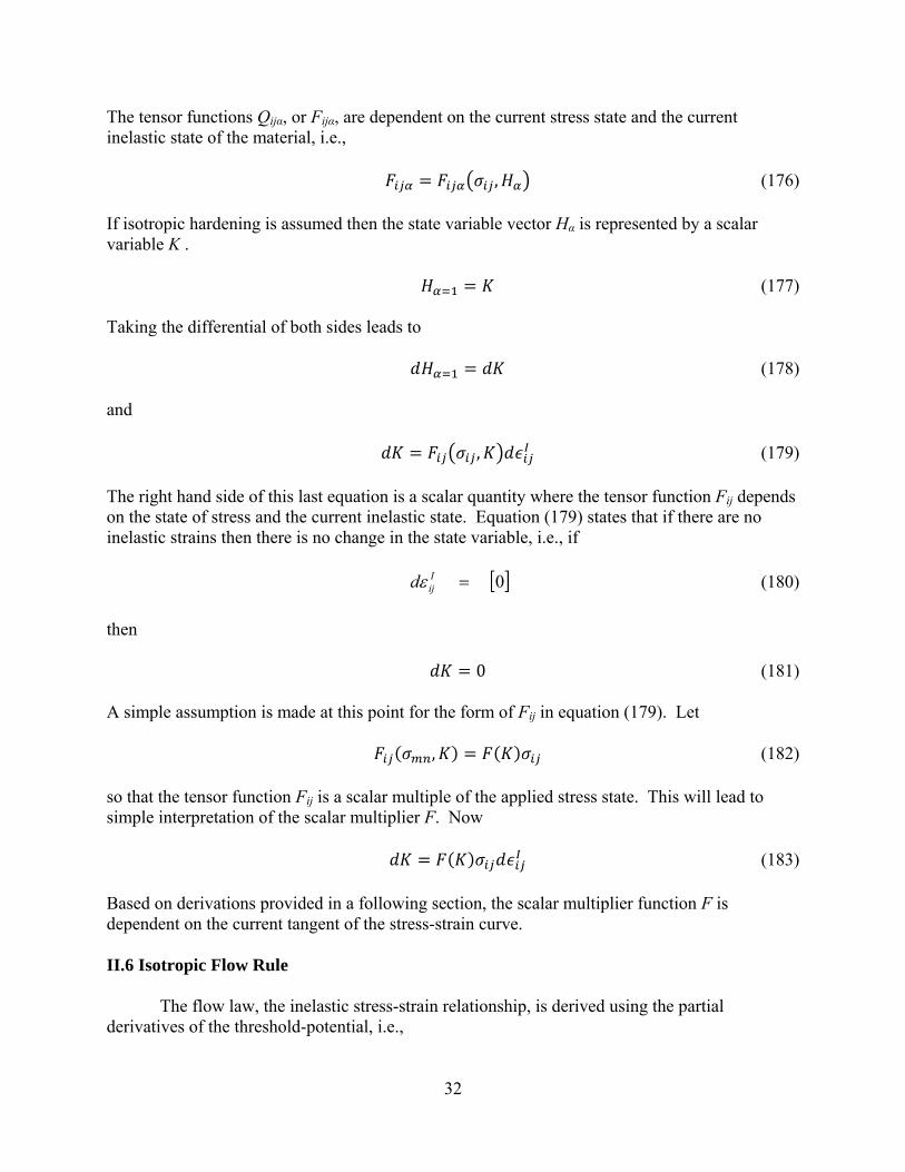
The tensor functions Qijα, or Fijα, are dependent on the current stress state and the current inelastic state of the material, i.e.,

, (176)

If isotropic hardening is assumed then the state variable vector Hα is represented by a scalar variable K .

(177)

Taking the differential of both sides leads to

(178)

and

, (179)

The right hand side of this last equation is a scalar quantity where the tensor function Fij depends on the state of stress and the current inelastic state. Equation (179) states that if there are no inelastic strains then there is no change in the state variable, i.e., if

0Iijd (180)

then

0 (181)

A simple assumption is made at this point for the form of Fij in equation (179). Let

, (182)

so that the tensor function Fij is a scalar multiple of the applied stress state. This will lead to simple interpretation of the scalar multiplier F. Now

(183)

Based on derivations provided in a following section, the scalar multiplier function F is dependent on the current tangent of the stress-strain curve.

II.6 Isotropic Flow Rule

The flow law, the inelastic stress-strain relationship, is derived using the partial derivatives of the threshold-potential, i.e.,

33

ij

iij

ij

Iij

Kafd

fdd

,, (184)

Recall that ai is a vector associated with the direction of the principle stresses. Equation (184) represents a flow rule that embodies the concept of normality, and by using the threshold function in this equation an associated flow rule is explicitly adopted. The gradient defines the direction of the increment of the inelastic strain vector and dλ defines the length.

Making use of the isotropic threshold function from Section II.1, recall that there are four functional forms of f and there are four partial derivatives of the function. Explicit formulations of these partial derivatives are given in equations (70), (71), (72), and (73). So the derivatives in equation (184) have been defined earlier. However, the scalar multiplier dλ needs defined and this is accomplished by developing an evolutionary law for the inelastic state variable. The evolutionary law is combined with the consistency condition to produce a mathematical expression

dKK

fd

fdf ij

ij

(185)

Note that the differential change in the unit vector, dai, is zero. Substituting equation (183) into equation (184) and solving for dλ yields

(186)

Substitution of equation (186) into equation (184) yields

(187)

Now define

(188)

then

(189)

where

34

(190)

What remains are the details associated with the substitution of the partial derivatives of the threshold potential function and the particular form for G.

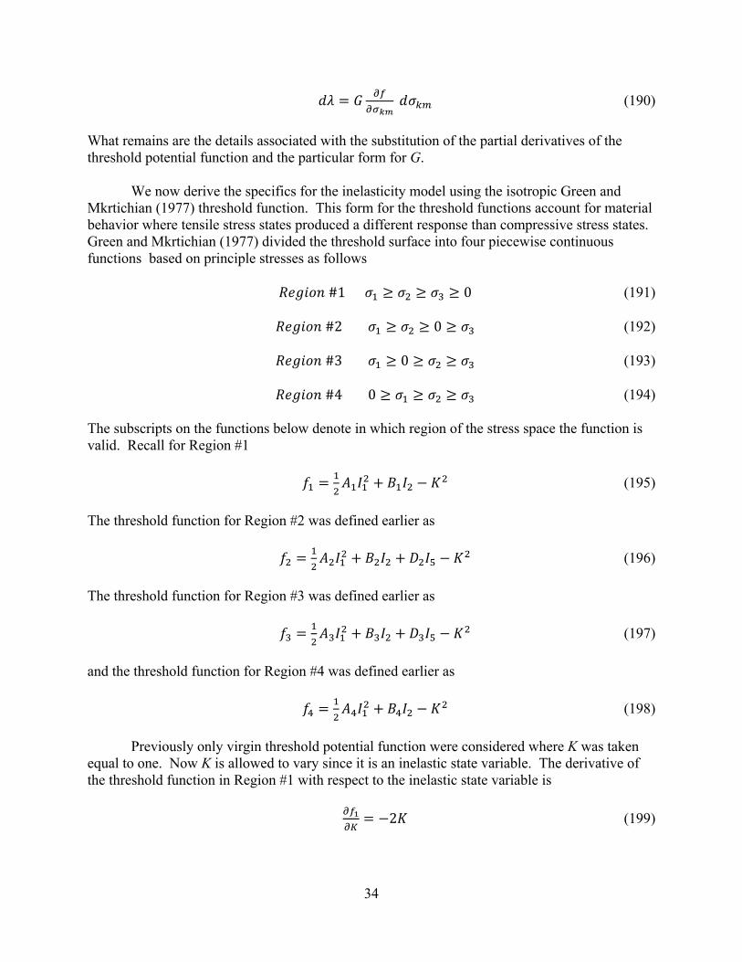
We now derive the specifics for the inelasticity model using the isotropic Green and Mkrtichian (1977) threshold function. This form for the threshold functions account for material behavior where tensile stress states produced a different response than compressive stress states. Green and Mkrtichian (1977) divided the threshold surface into four piecewise continuous functions based on principle stresses as follows

#1 0 (191)

#2 0 (192)

#3 0 (193)

#40 (194)

The subscripts on the functions below denote in which region of the stress space the function is valid. Recall for Region #1

(195)

The threshold function for Region #2 was defined earlier as

(196)

The threshold function for Region #3 was defined earlier as

(197)

and the threshold function for Region #4 was defined earlier as

(198)

Previously only virgin threshold potential function were considered where K was taken equal to one. Now K is allowed to vary since it is an inelastic state variable. The derivative of the threshold function in Region #1 with respect to the inelastic state variable is

2 (199)

35

Since isotropic hardening was assumed then similar derivatives with respect to K for Region #2, Region #3, and Region #4 are obtained, i.e.,

2 (200)

2 (201)

and

2 (202)

respectively.

Substituting the partial derivative of the isotropic formulation of f1 with respect to ij, (182), and (199) into equation (188) yields the following for Region #1

2 2 (203)

Substituting the partial derivative of the isotropic formulation of f2 with respect to ij, (182), and (200) into equation (188) yields the following for Region #2

2 2 2 (204)

Substituting the partial derivative of the isotropic formulation of f3 with respect to ij, (182), and (201) into equation (188) yields the following for Region #3

2 2 2 (205)

Substituting the partial derivative of the isotropic formulation of f4 with respect to ij, (182), and (202) into equation (188) yields the following for Region #4

2 2 (206)

The partial derivative of the isotropic formulation of the threshold function f1 with respect to ij and equation (203) are now substituted into (189) which yields

1 1 111 1 1 1 22

1 1 1 2

2

2 2ij ijI

ij

A I Bd A I dI B dI

KF A I B I

(207)

Substituting the partial derivative of the isotropic formulation of the threshold function f2 with respect to ij and equation (204) into equation (189) yields

36

2 1 2 222 1 1 2 2 2 52

1 1 1 2 2 5

2

2 2 2

ij ij m i jm j n niIij

A I B D a a a ad A I dI B dI D dI

KF A I B I D I

(208)

Substituting The partial derivative of the isotropic formulation of the threshold function f3 with respect to ij and equation (205) into equation (189) yields

3 1 3 333 1 1 3 2 3 52

3 1 3 2 3 5

2

2 2 2

ij ij m i jm j n niIij

A I B D a a a ad A I dI B dI D dI

KF A I B I D I

(209)

Substituting The partial derivative of the isotropic formulation of the threshold function f4 with respect to ij and equation (206) into equation (189) yields

4 1 444 1 1 4 22

4 1 4 2

2

2 2ij ijI

ij

A I Bd A I dI B dI

KF A I B I

(210)

Equations (207) through (210) comprise the inelastic flow law for each Region of the stress space.

II.7 The Scalar Function F(K) for Isotropy

For Region #1substituting the incremental strain tensor defined in equation (207) into the evolutionary law given by equation (183) leads to

2 (211)

Substituting equation (208) into equation (183) for Region #2 yields

2 (212)

Substituting equation (209) into equation (183) for Region #3 yields

2 (213)

Substituting equation (210) into equation (183) for Region #4 yields

2 (214)

Even though the assumption is made that the material hardens isotropically and only one state variable is required, there are four incremental evolutionary equations governing the behavior of the inelastic state variable K .

Now consider uniaxial tensile stress state where

37

0 0

0 0 00 0 0

(215)

The invariants for this stress state are

(216)

and

(217)

The strain increment for this inelastic stress state is

1 1 111 2

111 1 1 2

1

2 2I

klklt

f fd d

K F A I B I

(218)

Where the scalar function F is denoted as tF for this uniaxial load application. Solving this expression for tF yields

1 1

211 111 1 1 2

1

2 2kl

tkl

df fF

dK A I B I

(219)

Since σ11 is the only non-zero component of the stress tensor, then

1 1 11

211 11 111 1 1 2

1

2 2t

f f dF

dK A I B I

(220)

Substitution of the invariants I1 and I2 from above leads to

1 1 11

11

2

2t

A B dF

K d

(221)

In this expression the total derivative of σ11 with respect to d11 can be interpreted as the current tangent of the uniaxial stress-strain curve. This is not exact since the current slope is a derivative with respect to the total strain, but as the discussion below points out the approximation generates little error.

This slope of the current stress (σij) - total strain (ij) tot curve can be approximated using

the method developed by Ramberg–Osgood model where

38

0

1

2

n

tot

t

n

t

n

E E

CE

CE

(222)

Then the slope of the stress-strain curve can be calculated by taking the differential of both sides of equation (222), i.e.,

2

12

12

1

1

1

ntot

n

n

d d C dE

d nC dE

nC dE

(223)

Thus

1

2

1

1tot n

d

d E n C

(224)

Typically the reciprocal of Young’s modulus is small when compared to the rest of the denominator except for low values of stress where there is little inelastic strain and the response of the material is elastic. Thus for higher values of stress that are beyond the initial threshold values, the increment in strain is predominantly inelastic, and the increment in inelastic strain is given by

12

nId n C d (225)

Note that beyond the uniaxial threshold stress value any change in the total strain is due primarily to changes in the inelastic strain and

tot I

d d

d d

(226)

Figure 10 shows the above approximations and how closely the approximations match the data.

39

Figure 10 Computed Compressive Stress-Strain Curve for H-451 Graphite with Data

Next consider uniaxial compression stress where

0 0

0 0 00 0 0

(227)

The invariants for this stress state are

(228)

and

(229)

Denoting the scalar function F as cF then

4 4 411 2

114 1 4 2

1

2 2I

kmkmc

f fd d

K F A I B I

(230)

Solving for F

40

4 4

211 114 1 4 2

1

2 2km

ckm

df fF

dK A I B I

(231)

Since σ11 is the only non-zero component of the stress tensor, then

4 4 11

211 11 114 1 4 2

1

2 2c

f f dF

dK A I B I

(232)

which simplifies to

4 4 11

11

2

2c

A B dF

K d

(233)

This last equation is different than the corresponding equation for tension again accounting for different properties between tension and compression.

41

234

235

236

42

237

238

239

43

240

241

44

II.8 Anisotropic Formulation

Once again the flow law is derived from the threshold potential function by way of the derivative following of the threshold function

(242)

where dλ is the scalar quantity that defines the length of the gradient vector. For anisotropy Equation (242) represents a flow rule that embodies the concept of normality, and by using the threshold function in this equation an associated flow rule is explicitly adopted. The gradient defines the normal to the threshold surface and this normal defines the direction of the increment of the inelastic strain vector.

, , , (243)

Recall the ai is a vector associated with the direction of the principle stresses and the di vector is associated with the preferred material direction for transverse isotropy.

The gradients to the threshold surface are given in equations (151), (152), (153), and (154). These functions account for the different material behavior in tension and compression as well as the directional properties of certain types of graphite. The threshold surface is once again divided into four piecewise continuous functions based on principle stresses as follows.

Region#1 σ1 ≥ σ2 ≥ σ3 ≥ 0 (244)

Region#2 σ1 ≥ σ2 ≥ 0 ≥ σ3 (245)

Region#3 σ1 ≥ 0 ≥ σ2 ≥ σ3 (246)

Region#4 0 ≥ σ1 ≥ σ2 ≥ σ3 (247)

The subscript on the function denotes which region of the stress space the function is valid. Thus for Region #1

(248)

The threshold function defined for Region #2 is

(249)

The threshold function defined for Region #3 is

(250)

45

and the threshold function defined for Region #4 is

(251)

The inelastic state variable K is allowed to vary. Thus the derivative of the threshold function in Region #1 with respect to the inelastic state variable is

2 (252)

Since isotropic hardening was assumed then similar derivatives with respect to K for Region #2, Region #3 and Region #4 are obtained, i.e.,

2 (253)

2 (254)

and

2 (255)

respectively

Substituting equations (124), (182), and (252) into equation (188) yields the following for Region #1

2 2 2 2 (256)

Substituting equations (125), (182), and (253), and into equation (188) yields the following for Region #2

2 2 2 2 2 2 (257)

Substituting equations (126), (182), and (254) into equation (188) yields the following for Region #3

2 2 2 2 2 2 (258)

Substituting equations (127), (182), and (255) into equation (188) yields the following for Region #4

2 2 2 2 (259)

The expressions for the scalar function F has yet to be determined.

46

Now we concentrate on the components of the incremental strain relationship from equation (189). Equations (124) and (256) are substituted into (189) such that

1 1 1 6 1 1 1 111 1 1 6 12

1 1 1 2 1 1 6 1 7

1 2 1 1 6 1 7

2

2 2 2 2

ij ij i j p j ip j q qiIij

A I E I B E I d d F d d d dd A I E I dI

KF A I B I E I I F I

B dI E I dI F dI

(260)

Substituting equations (125) and (257) into equation (189) yields

22 1 2 62

2 1 2 2 2 5 2 1 6 2 7 2 9

2 2 2 1 2

2 2 1 2 6 1

2 2 2 5 2 1 6 2 7 2 9

1

2 2 2 2 2 2

2

Iij ij

ij m i jm j n ni i j k j ik j n ni

p q q i jp i q q r rj

d A I E IKF A I B I D I E I I F I H I

B D a a a a E I d d F d d d d

H a a d d a a d d A I E I dI

B dI D dI E I dI F dI H dI

(261)

Substituting equations (126) and (258) into equation (189) yields

33 1 3 62

3 1 3 2 3 5 3 1 6 3 7 3 9

3 3 3 1 3

3 3 1 3 6 1

3 2 3 5 3 1 6 3 7 3 9

1

2 2 2 2 2 2

2

Iij ij

ij m i jm j n ni i j k j ik j n ni

p q q i jp i q q r rj

d A I E IKF A I B I D I E I I F I H I

B D a a a a E I d d F d d d d

H a a d d a a d d A I E I dI

B dI D dI E I dI F dI H dI

(262)

Substituting equations (127) and (259) into equation (189) yields

4 1 4 6 4 4 1 444 1 4 6 12

4 1 4 2 4 1 6 4 7

4 2 4 1 6 4 7

2

2 2 2 2

ij ij i j p j ip j q qiIij

A I E I B E I d d F d d d dd A I E I dI

KF A I B I E I I F I

B dI E I dI F dI

(263)

Equations (260) through (263) comprise the inelastic flow law for each Region of the stress space.

II.9 The Scalar Function F(K) for Anisotropy

Modeling inelastic stress-strain behavior by substituting the incremental strain equation (260) into the evolutionary law equation (183) for Region #1 leads to the following expression

47

2 (264)

Substituting equation (261) into the evolutionary law equation (183) for Region #2 yields

2 (265)

Substituting equation (262) into the evolutionary law equation (183) for Region #3 yields

2 (266)

Substituting equation (263) into the evolutionary law equation (183) for Region #4 yields

2 (267)

As was the case for isotropic graphite, for anisotropic graphite there are four separate incremental formulations for the isotropic state variable K.

Next consider a uniaxial tensile stress where

0 0

0 0 00 0 0

(268)

The invariants for this stress state are

(269)

(270)

(271)

and

(272)

The inelastic strain increment for this state of stress is

1 1 111 2

111 1 1 2 1 1 6 1 7

1

2 2 2 2I

klkl

f fd d

K F A I B I E I I F I

(273)

Solving for F yields

1 1

211 111 1 1 2 1 1 6 1 7

1

2 2 2 2klI

kl

df fF

dK A I B I E I I F I

(274)

48

Since σ11 is the only non-zero component of the stress tensor, then

1 1 11

211 11 111 1 1 2 1 1 6 1 7

1

2 2 2 2 I

f f dF

dK A I B I E I I F I

(275)

Simplifying

111 1 1 1 1 1 1 1

11

12 2 2

2 I

dF A B E d d Fd d

K d

(276)

Note that the term dσkl is the slope of the stress strain curve beyond yielding for the associated direction vector di. The derivative of stress with respect to inelastic strain is approximated using by the Ramberg-Osgood uniaxial stress-strain law.

49

278

277

50

280

279

51

282

281

52

284

283

53

III. Reliability Model

The purpose of this segment of the project was establishing a single form invariant probabilistic based failure model for components fabricated from graphite. The probabilistic failure model must reflect the material behavior of graphite. Through the application of invariant theory and the Cayley-Hamilton theorem as outlined in Spencer (1984), an integrity basis with a finite number of stress invariants will be formulated that reflects the material behavior of graphite. The integrity basis, when posed properly, spans the functional space for the failure model. A model based on a linear combination of stress invariants will capture the material behavior in a mathematically convenient manner. This effort begins by proposing a deterministic failure criterion that reflects relevant material behavior. When the model parameters are treated as random variables, a deterministic model can be transformed into a probabilistic failure model. Monte Carlo simulation with importance sampling will be used to compute component failure probabilities. The three classical models will be compared with the experiment results obtained from Burchell (2007).

III.1 Graphite Failure Data

In the following section several common failure criterion models will be introduced and the constants for the models are characterized using biaxial failure data generated by Burchell (2007). For the simpler models Burchell’s (2007) data has more information than is necessary. For some models all the constants cannot be approximated because there is not enough appropriate data for that particular model. These issues are identified for each failure model. Burchell’s specimens were fabricated from grade H-451 graphite. There were nine load cases presented, including two uniaxial tensile load paths along two different material directions (data suggests that the material is anisotropic), one uniaxial compression load path, and six biaxial stress load paths. The test data is summarized in Table 1. The mean values of the normal stress components for each load path from Burchell’s (2007) data are presented in Table 2. In addition, corresponding invariants are calculated and presented in Table 2 along with Lode’s angle. All the load paths are identified in Figure 11.

54

Table 1 Grade H-451 Graphite: Load Paths and Corresponding Failure Data

Data Set Ratio

Failure Stresses (MPa）

# B-1 1 : 0

10.97 0

9.90 0

9.08 0

9.22 0

12.19 0

11.51 0

# B-2 0 : 1

0 15.87

0 12.83

0 18.06

0 20.29

0 14.32

0 14.22

# B-3 0 : - 1

0 -47.55

0 -50.63

0 -59.72

0 -56.22

0 -48.19

0 -51.54

# B-4 1 : - 1

9.01 -8.94

7.68 -7.68

14.34 -14.16

8.93 -8.78

13.23 -13.14

9.21 -9.11

Data Set Ratio

Failure Stresses (MPa）

# B-5 2 : 1

7.81 3.57

8.54 3.89

11.2 5.6

13.00 6.42

11.54 5.76

12.12 6.03

# B-6 1 : 2

6.36 12.67

6.42 12.86

6.74 13.42

7.69 15.36

6.46 12.95

7.17 14.36

# B-7 1 : - 2

7.98 -15.99

5.50 -10.96

6.69 -13.37

10.49 -21.01

9.18 -18.30

11.31 -22.61

Data Set Ratio

Failure Stresses (MPa）

# B-8 1 : 1.5

6.69 10.03

6.51 9.78

8.07 12.11

9.13 13.74

6.11 9.19

9.24 13.91

9.93 14.93

8.93 13.41

7.20 10.79

# B-9 1 : - 5

6.35 -31.61

8.69 -43.44

7.40 -36.86

7.09 -35.30

5.94 -29.50

6.83 -32.83

8.06 -40.21

7.75 -38.58

55

Figure 11 Burchell’s (2007) Load Paths Plotted in a 1 – 2 Stress Space

Table 2 Invariants of the Average Failure Strengths for All 9 Load Paths

Data Set (1)ave (MPa) (2)ave (MPa) (MPa) r (MPa)

# B-1 10.48 0 6.05 8.56 0.00o

# B-2 0 15.93 9.20 13.01 0.00 o

# B-3 0 -52.93 -30.56 43.22 60.00 o

# B-4 10.4 -10.3 0.06 14.64 29.84 o

# B-5 10.7 5.21 9.19 7.57 29.13 o

# B-6 6.81 13.6 11.78 9.62 30.05o

# B-7 8.53 -17.04 -4.91 18.41 40.88 o

# B-8 7.98 11.99 11.53 8.63 40.82 o

# B-9 7.26 -36.04 -16.62 32.79 50.99 o

)(2 MPa

)(1 MPa

#B-3

#B-9

#B-7

#B-4

#B-5

#B-8 #B-6

#B-1

#B-2

56

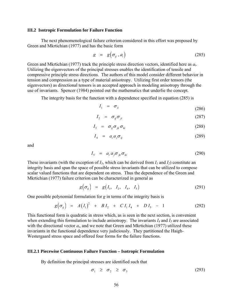
III.2 Isotropic Formulation for Failure Function

The next phenomenological failure criterion considered in this effort was proposed by Green and Mkrtichian (1977) and has the basic form

,ij ig g a (285)

Green and Mkrtichian (1977) track the principle stress direction vectors, identified here as ai. Utilizing the eigenvectors of the principal stresses enables the identification of tensile and compressive principle stress directions. The authors of this model consider different behavior in tension and compression as a type of material anisotropy. Utilizing first order tensors (the eigenvectors) as directional tensors is an accepted approach in modeling anisotropy through the use of invariants. Spencer (1984) pointed out the mathematics that underlie the concept.

The integrity basis for the function with a dependence specified in equation (285) is

(286)

jiijI 2 (287)

kijkijI 3 (288)

ijji aaI 4 (289)

and

kijkji aaI 5 (290)

These invariants (with the exception of I3, which can be derived from I1 and I2) constitute an integrity basis and span the space of possible stress invariants that can be utilized to compose scalar valued functions that are dependent on stress. Thus the dependence of the Green and Mkrtichian (1977) failure criterion can be characterized in general as

1 2 4 5, , ,ijg g I I I I (291)

One possible polynomial formulation for g in terms of the integrity basis is

2

1 2 1 4 5 1ijg A I B I C I I D I (292)

This functional form is quadratic in stress which, as is seen in the next section, is convenient when extending this formulation to include anisotropy. The invariants I4 and I5 are associated with the directional vector ai, and we note that Green and Mkrtichian (1977) utilized these invariants in the functional dependence very judiciously. They partitioned the Haigh-Westergaard stress space and offered four forms for the failure functions.

III.2.1 Piecewise Continuous Failure Function – Isotropic Formulation

By definition the principal stresses are identified such that

321 (293)

iiI 1

57

The four functions proposed by Green and Mkrtichian (1977) span the stress space which is partitioned as follows:

Region #1: 0321 – all principal stresses are tensile

Region #2: 321 0 – one principal stress is compressive, the others

are tensile

Region #3: 321 0 – one principal stress is tensile, the others are

compressive

Region #4: 3210 – all principal stresses are compressive.

Thus the Green and Mkrtichian (1977) criterion has a specific formulation for the case of all tensile principle stresses, and a different formulation for all compressive principle stresses (see derivation below). For these two formulations there is no need to track principle stress orientations and thus for Regions #1 and #4 the Green and Mkrtichian (1977) failure criterion did not include the terms associated with I4 and I5, both of which contain information regarding the directional tensor. A third and fourth formulation exists for Regions #3 and #4 where two principle stresses are tensile and when two principle stresses are compressive, respectively and the failure behavior depends on the direction of the principal tensile and compressive stresses. For these regions of the stress space for the Green and Mkrtichian (1977) failure criterion includes the invariants I4 and I5.

The functional values of the four formulations g1, g2, g3 and g4 must match along their common boundaries. In addition, the tangents associated with the failure surfaces along the common boundaries must be single valued. This will provide a smooth transition from one region to the next. To insure this, the gradients to the failure surfaces along each boundary are equated. The specifics of equating the formulations and equating the gradients at common boundaries are presented below. Relationships are developed for the constants associated with each term of the failure function for the four different regions.

Region #1: 0321 Green and Mkrtichian (1977) assumed the failure

function for this Region of the stress space is

21 1 1 1 2

11

2g A I B I

(294)

From equation (294) it is evident that there will be a group of constants for each region of the stress space. Hence the subscripts for the constants associated with each invariant as well as the failure function will run from one to four. Also note the absence of invariants I4 and I5. The corresponding gradient to the failure surface is

1 1 1 1 2

1 2ij ij ij

g g I g I

I I

(295)

where

11 1

1

gA I

I

(296)

58

11

2

gB

I

(297)

ijij

I

1 (298)

and

ijij

I

22 (299)

Here ij is the Kronecker delta tensor. Substitution of equations (296) through (299) into (295) leads to the following tensor expression

11 1 12ij ij

ij

gA I B

(300)

or in a matrix format

(301)

The matrix formulation allows easy identification of relationships between the various constants.

Region #2: 321 0 The failure function for Region #2 is

22 2 1 2 2 2 1 4 2 5

1

2g A I B I C I I D I

(302)

Note the subscripts on the constants and the failure function. The gradient to the surface is

52 2 1 2 2 2 4 2

1 2 4 5ij ij ij ij ij

Ig g I g I g I g

I I I I

(303)

Here

22 1 2 4

1

gA I C I

I

(304)

22

2

gB

I

(305)

22 1

4

gC I

I

(306)

22

5

gD

I

(307)

1

3

2

1

1

321

321

321

1

200

020

002

00

00

00

BAf

ij

59

jiij

aaI

4 (308)

and

kikjjkikij

aaaaI

5 (309)

The principle stress direction of interest in this region of the stress space is the one associated with the third principal stress. Assuming the Cartesian coordinate system is aligned with the principal stress directions then the eigenvector associated with the third principal stress is

)1,0,0(ia (310)

Thus for equation (307) and (308)

100

000

000

100

1

0

0

jikjik aaaaaa

(311)

Given the principle stress direction the fourth and fifth invariants are

34 I (312)

and

235 I (313)

for this region of the stress space. Substitution of equations (304) through (308) into (303) yields the following tensor expression for the normal to the failure surface

2

2 1 2 2 3 1

2

2 ( )

( )

ij ij ij i iij

k i jk j k ki

gA I B C I a a

D a a a a

(314)

The matrix form of equation (314) is

1 2 3 1

21 2 3 2 2 2

1 2 3 3

3

3 2 2

1 2 3 3

0 0 2 0 0

0 0 0 2 0

0 0 0 0 2

0 0 0 0 0

0 0 0 0 0

0 0 2 0 0 2

ij

gA B

C D

(315)

60

Region #3: 321 0 The failure function for this region of the stress

space is

23 3 1 3 2 3 1 4 3 5

1

2g A I B I C I I D I

(316)

The normal to the surface is

3 3 3 3 3 51 2 4

1 2 4 5ij ij ij ij ij

g g g g g II I I

I I I I

(317)

Here

33 1 3 4

1

gA I C I

I

(318)

33

2

gB

I

(319)

33 1

4

gC I

I

(320)

and

33

5

gD

I

(321)

The principle stress direction of interest for this stress state is the one associated with the first principal stress, i.e.,

)0,0,1(ia (322)

Now

000

000

001

001

0

0

1

jikjik aaaaaa

(323)

The fourth and fifth invariants for this Region of the stress space are

14 I (324)

and

215 I (325)

Substitution of the quantities specified above into (317) yields the following tensor expression

61

33 1 3 3 1 1

3

2 ( )

( )

ij ij ij i jij

k i jk j k ki

gA I B C I a a

D a a a a

(326)

The matrix form of this equation is as follows

1 2 3 1

31 2 3 3 2 3

1 2 3 3

1 2 3 1

1 3 3

1

0 0 2 0 0

0 0 0 2 0

0 0 0 0 2

2 0 0 2 0 0

0 0 0 0 0

0 0 0 0 0

ij

gA B

C D

(327)

Region #4: ( 3210 ) The failure function for this region of the

stress space is

24 4 1 4 2

11

2g A I B I

(328)

The corresponding normal to the failure surface is

4 4 1 4 2

1 2ij ij ij

g g I g I

I I

(329)

Here

44 1

1

gA I

I

(330)

and

44

2

gB

I

(331)

Substitution of the equations above into (329) yields the following tensor expression

44 1 42ij ij

ij

gA I B

(332)

The matrix format of this expression is

1 2 3 1

41 2 3 4 2 4

1 2 3 3

0 0 2 0 0

0 0 0 2 0

0 0 0 0 2ij

gA B

(333)

With the failure functions and the gradients to those functions defined for each region, attention is now turned to defining the constants. Consider the region of the Haigh-Westergaard stress space where with andThe stress state in a matrix format is

62

000

00

00

2

1

ij (334)

and this stress state lies along the boundary shared by Region #1 and Region #2. At this boundary we impose

1 2g g (335)

and

1 2

ij ij

g g

(336)

For this stress state the invariants I1 and I2 are

211 I (337)

and

22

212 I (338)

for both g1 and g2. The invariants I4 and I5 for g2 are

034 I (339)

and

0235 I (340)

Substitution of equations (337) through (340) into equation (336) yields the following matrix expression

22

21

22

1

2

21

21

21

12

1

1

21

21

21

000

000

000

00

000

000

000

020

002

00

00

00

000

020

002

00

00

00

DC

BA

BA

(341)

The following three expressions can be extracted from equation (341)

2122111121 2)(2)( BABA (342)

2222112121 2)(2)( BABA (343)

221221121 )()()( CAA (344)

63

The constant D2 does not appear due to its multiplication with the null matrix. However, C2 does appear in the third expression but in the first two immediately above. Focusing on equation (342) and equation (343) which represents two equations in two unknowns then

21 BB (345)

and

21 AA (346)

Substitution of equation (346) into equation (344) yields

02 C (347)

and at this point D2 is indeterminate

Now consider the Region of the Haigh-Westergaard stress space where and The stress state in a matrix format is

3

1

00

000

00

ij

(348)

and this stress state lies at the boundary shared by Region #2 and Region #4. At this boundary we impose

2 3g g (349)

and

32

ij ij

gg

(350)

Under these conditions the invariants I1 and I2 are

311 I (351)

and

23

212 I (352)

Substitution of equation (351) and (352) into equation (350) yields

64

3

1

3

1

1

31

3

3

1

3

31

31

31

2

3

2

31

3

3

2

3

1

2

31

31

31

000

000

002

00

00

002

200

000

002

00

00

00

200

000

000

200

00

00

200

000

002

00

00

00

DC

BA

DC

BA

(353)

The following three expressions can be extracted from equation (353)

3133131331

2321231

222)(

2)(

DCBA

CBA

(354)

3133123231 )()( CACA (355)

and

3133331

2323123231

2)(

222)(

CBA

DCBA

(356)

Earlier it was determined that C2 = 0, so from equation (355) we obtain

331

332 )(

CAA

(357)

From equation (354) and equation (355) we obtain

331

3132 2

)(DCBB

(358)

In addition, from equation (356) and equation (355) we obtain

331

312 2

)(DCD

(359)

Consider the Region of the Haigh-Westergaard stress space where and The stress sate in a matrix format is

65

3

2

00

00

000

ij

(360)

and this stress state lies along the boundary shared by Region #3 and Region #4. At this boundary we impose

3 4g g (361)

and

3 4

ij ij

g g

(362)

Under these conditions the invariants I1 and I2 are

321 I (363)

and

23

222 I (364)

Substitution of equations (367) and (368) into equation (366) yields

4

3

24

32

32

32

33

32

3

3

23

32

32

32

200

020

000

00

00

00

000

000

000

000

000

00

200

020

000

00

00

00

BA

DC

BA

(365)

The following three expressions can be extracted from equation (365)

432332332 )()( ACA (366)

4243232332 2)(2)( BABA (367)

and

4343233332 2)(2)( BABA (368)

From equation (366) we discern that

433 ACA (369)

From equation (367) and equation (368) we obtain

66

432332 2222 BB (370)

or that

43 BB (371)

Substitution of equations (369) and (370) into equation (367) leads to

43 AA (372)

and

03 C (373)

Substitution of equation (373) into equations (355), (356) and (357) yields

32 AA (374)

332 DBB (375)

and

32 DD (376)

So the relationships between the functional constants are as follows

4321 AAAA (377)

242321 DBDBBB (378)

032 CC (379)

and

032 DD (380)

These relationships insure that the four functional forms for the failure function are smooth and continuous along the boundaries of the four regions.

III.2.2 Definition of Failure Function Constants – Isotropic Failure

Next we utilize specific load paths in order to define the constants defined above in terms of stress values obtained at failure. Consider the following stress state at failure under a uniaxial tensile load

000

00

000

Tij (381) 1x

2x

3x

T

T

67

This stress state lies on the boundary of Region #1. The invariants for this stress state are

TI 1 (382)

and

22 TI (383)

The failure function takes the form

2 2

1 1 1

11

20

T Tg A B

(384)

from which the following relationship is obtained

211

1

2

1

T

BA

(385)

Next a uniaxial compressive stress state is considered where

C00

000

000

ij (386)

The principle stress direction for this stress state is

)1,0,0(ia (387)

thus

100

000

000

ji aa (388)

The invariants are as follows

CI 1 (389)

22 CI (390)

CI 4 (391)

1x

2x

3x

C

C

68

and

25 CI (392)

Thus

2 2 2

2 2 2 2

11

20

C C Cg A B D

(393)

which leads to

2222

1

2

1

C

DBA

(394)

Next consider an equal biaxial compressive stress state where

BC

BC

-00

0-0

000

ij (395)

This stress state lies within Region #4 and the invariants are as follows

BCI 21 (396)

and

22 2 BCI (397)

The failure function for this particular stress state is

2 2

4 4 4

12 2 1

20

BC BCg A B

(398)

which leads to

244

2

1

BC

BA

(399)

Solving equations (385), (394) and (399) using equations (377) through (380) leads to

1x

2x

3x

BC

BC

BCBC

69

224321

21

CBC

AAAA

(400)

22221

1

2

11

CBCT

BB

(401)

2243

2

12

BCC

BB

(402)

and

2232

11

TC

DD

(403)

In order to visualize the isotropic version of the Green and Mkrtichian (1977) failure criterion relative to Burchell’s (2007) failure data, values were computed for the strength constants immediately above, i.e., T = 15.93 MPa for tension, C = 52.93 MPa for compression and BC = 61.40 MPa for the biaxial compression. The values for T and C and were obtained directly from Burchell’s (2007) data. The value for BC was determined by a best fit approximation of the failure curve to the data in Figure 12. Various projections of the isotropic Green and Mkrtichian (1977) failure criterion are presented in the next several figures along with the Burchell (2007) data. The first is a projection onto the 1 – 2 stress space which is depicted in Figure 12. As can be seen in this figure the isotropic Green and Mkrtichian (1977) model captures the different behavior in tension and compression exhibited by the Burchell (2007) data along the 2 axis. However, the Green and Mkrtichian (1977) failure criterion does not capture material anisotropy which is clearly exhibited by the Burchell (2007) failure data along the tensile segments of the 1 axis relative to the 2 axis.

70

Figure 12 The Green-Mkrtichian (1977) failure criterion projected onto the 1 -2 principle stress plane (T= 15.93 MPa, C = 52.93 MPa, BC = 61.40 MPa)

The isotropic Green and Mkrtichian (1977) failure criterion is projected onto the deviatoric planes in Figures 13 and 14. Note that a cross section through the failure function perpendicular to the hydrostatic axis transitions from a pyramidal shape (Figure 14) to a circular shape (Figure 13) with an increasing value of the stress invariant I1. This suggests that the apex of the failure function presented in a full Haigh-Westergaard stress space is blunt, i.e., quite rounded for the this particular criterion.

71

Figure 13 The Green-Mkrtichian criterion projected onto a deviatoric plane MPa20.9

parallel to the -plane with T = 15.93 MPa, C = 52.93 MPa, BC = 61.40 MPa

Figure 14 The Green-Mkrtichian criterion projected onto a deviatoric plane MPa2.30

parallel to the -plane with T = 15.93 MPa, C = 52.93MPa, BC = 61.40 MPa

The meridian lines of the isotropic Green-Mkrtichian (1977) failure surface corresponding to o0 and o60 are depicted on Figure 15. Obviously the meridian lines are not linear. The o0 meridian line goes through point defined by 9.02 MPa and r = 13.01

72

MPa. The o60 meridian line goes through the point defined by = 30.56 MPa and r = 43.22 MPa.

Figure 2.7.4 The Green-Mkrtichian criterion projected onto the meridian plane for a material strength parameter of T = 15.93 MPa, C = -52.93 MPa, BC = -61.40 MPa

Figure 15 Different meridian curves of the isotropic Green-Mkrtichian (1977) criterion (T = 15.93 MPa, C = 52.93 MPa, BC = 61.40 MPa)

As the value of the I1 stress invariant associated with the hydrostatic stress increases in the negative direction, failure surfaces perpendicular to the hydrostatic stress line become circular again. The model suggests that as hydrostatic compression stress increases the difference between tensile strength and compressive strength diminishes and approach each other asymptotically. This is a material behavior that should be verified experimentally in a manner similar to Bridgman’s (1953) bend bar experiments conducted in hyperbaric chambers on cast metal alloys. Balzer (1998) provides an excellent overview of Bridgman’s experimental efforts, as well as others and their accomplishments in the field of high pressure testing.

)(MPa

)(MParo30

o60

o0)0,13.50,9.70(),,( o

BC MPaMPar

)60,33.43,56.30(),,( oC MPaMPar

)0,01.13,02.9(),,( oT MPaMPar

73

Figure 16 Different deviatoric planes from the isotropic Green-Mkrtichian (1977) failure criterion with nine average strength values from Burchell’s (2007) failure data.

(T = 15.93 MPa, C = 52.93 MPa, BC = 61.40 MPa, see Table 2).

III.2 Anisotropic Formulation

As discussed in earlier sections the Burchell (2007) multiaxial failure data strongly suggests that the graphite tested was anisotropic. Thus there is a need to extend the isotropic failure model discussed in the previous section so that anisotropic failure behavior is captured. This can be done again by utilizing stress based invariants where the material anisotropy is captured through the use of a direction vector associated with primary material directions. The concept is identical to the extension of the isotropic inelastic constitutive model presented earlier in this report. The extension of a phenomenological failure criterion will be made for a transversely isotropic material. Other material symmetries, e.g., an orthotropic material symmetry, can be included as well. Duffy and Manderscheid (1990b) as well as others have suggested an appropriate integrity basis for the orthotropic material symmetry. Transversely isotropic materials have the same properties in one plane and different properties in a direction normal to this plane. Orthotropic materials have different properties in three mutually perpendicular directions.

The preferred material direction is designated through a second direction vector, di. The dependence of the failure function is extended such that

0,, jijiij aaddg (404)

The definition of the unit vector ai is the same as in earlier sections. Rivlin and Smith (1969) as well as Spencer (1971) show that for a scalar valued function with dependence stipulated by equation (404) the integrity basis is

)(1 MPa

)(2 MPa plane03

74

(405)

(406)

(407)

(408)

(409)

(410)

(411)

(412)

and

(413)

The invariant I3 is omitted again since this invariant is cubic in stress. As before those invariants linear in stress enter the functional dependence as squared terms or as products with another invariant linear in stress. Therefore the anisotropic failure function has the following dependence

9817

6154122

1

98765421

211

,,,,,,,,,

HIIGIFI

IEIDIICIBIIA

IIIIIIIIgaaddg jijiij

(414)

The form of the failure function was constructed as a polynomial in the invariants listed above. The constants in this formulation (A, B, C, D, E, F, G, and H) are characterized by adopting simple strength tests. The proposed failure function was incorporated into a reliability model through the use of Monte Carlo simulation and importance sampling techniques. This feature is discussed in a subsequent section.

Similar to the approach adopted for anisotropic constitutive models, the underlying concept is that the response of the material depends on the stress state, a preferred material direction and whether the principal stresses are tensile or compressive. The principle stress space is divided again into four regions. The regions and associated failure functions are listed below. In the first region where all of the principle stresses are tensile, i.e.,

Region #1: 0321

7161121

2111 2

11 IFIIEIBIAg (415)

In Region #1 a direction vector associated with the principle stresses is unnecessary since all principle stresses are tensile.

75

Region #2: 321 0

92812

7261252412222

122 211

IHIIG

IFIIEIDIICIBIAg

(416)

In Region #2 the direction vector ai is associated with the compressive principle stress σ3. Thus for this region

0, 0, 1 (417)

Region #3: 321 0

The failure function for this region of the stress space is

93813

7361353413232

133 211

IHIIG

IFIIEIDIICIBIAg

(418)

In Region #3 the direction vector ai is associated with the tensile principle stress direction σ1. For this region

1, 0, 0 (419)

Region #4: 3210

The failure function for this region of the stress space is

74614242

144 211 IFIIEIBIAg (420)

and since all principle stresses are compressive a direction vector associated with the principle stress direction is unnecessary.

Following derivations outlined earlier the coefficients for the four failure functions (i.e., g1. g2. g3. and g4) are defined by the following expressions

224321

12

BCTC

AAAA

(421)

222

343321

2

111

BCTCTT

DBDBBB

(422)

76

2232

11

TCTT

DD

(423)

22224321

1111

MBCYCBCTC

EEEE

(424)

222222

343321

111111

MBCYCYTBCTCTT

HFHFFF

(425)

222232

1111

YCYTTCTT

HH

(426)

where the strength parameters identified above are defined as

YT – tensile strength in the preferred material direction

YC – compressive strength in the preferred material direction

TT – tensile strength in the plane of isotropy

TC – compressive strength in the plane of isotropy

BC – equal biaxial compressive strength in the plane of isotropy

MBC – equal biaxial compressive strength with only one stress component in the plane of isotropy

The anisotropic Green and Mkrtichian (1977) failure criterion is projection onto the 1 – 2 stress space in Figure 17. The strength parameters were for the most part once again extracted from Burchell’s (2007) data. Values for the strength parameters listed above are given in the figure caption. Note the agreement with the data along the two tensile axes, as well as along the failure curve for each load path. Average strength values for each load path are depicted as open red circles in the figure.

77

Figure 17 Anisotropic Green-Mkrtichian (1977) failure criterion with Burchell’s (2007) failure data projected onto the 11 - 22 principle stress plane (TT = 10.48 MPa, TC = 35MPa,

BC = 40 MPaYC = 15.93 MPa, YC = 52.93 MPa, MBC = 61.40 MPa)

III.3 Monte Carlo Methods Using Importance Sampling

In general the probability of failure of a structural component can be expressed as

f

f YP f y dy

(427)

Here Y is a random strength variable, fY is a probability density function associated with t he random strength variable and δf is the failure domain that satisfies the expression

0g y (428)

where g(y) is the functional representation of the failure criterion. Although the integral seems straight forward, closed form solutions are unavailable except for simple failure criterion. As an alternative, conventional Monte Carlo simulation is commonly used to numerically evaluate the probability of failure when a closed form solution is difficult to formulate.

0,48.10, 21 MPa MPa93.15,0, 21

0,35, 21 MPa

)(11 MPa

MPaMPa 4.61,4.61

, 21

MPa93.52,0, 21

)(22 MPa

78

Monte Carlo simulation is relatively easy to implement. An indicator function I is defined such that

1 0

0 0

g yI

g y

(429)

This indicator function can be included in the integral above if the integration range is expanded to include the entire design variable space. Thus

s f

fP I f y dy

(430)

where earlier δs was defined as the safe domain of the design variable space. The integral on the right side of this expression defines the expectation of the indicator function, i.e.,

s f

E I I f y dy

(431)

Recall from statistics that the definition of the mean (μ) of a random variable (say X) is the expectation of the variable. Thus

x x f x dx

(432)

Also recall that the mean associated with a random variable can be estimated from a sample taken from the population that is being characterized by the distribution function f(x). The estimated value of the mean is given by the simple expression

1

1 N

x jj

xN

(433)

Where xj is the jth observation in a random sample taken from the population. In a similar fashion the probability of failure (Pf) represents the mean (or expected value) of the indicator function. Thus equation (430) can be expressed as

1

1lim

N

f jN j

P IN

(434)

Here it is implied that a random sample of successes (I = 1) or failures (I = 0) has been generated. Thus Ij is the jth evaluation of the limit state function where the random observations have been generated from the cumulative distribution function FX.

As noted above Monte Carlo simulation is computationally simple. To increase the accuracy of this numerical integration method the number of samples is simply increased. However, the method does not converge to correct answers in the low probability of failure regime. As engineers we wish to design components with very low probabilities of failure. Thus conventional Monte Carlo simulation is modified using importance sampling to achieve this goal. With importance sampling the design space is sampled only within the near vicinity of the most

79

probable point (MPP – see Figure 18). The name for the technique is derived from the notion that more sampling should take place in the most "important" region of the design variable space. The important region of the design variable space corresponds to the MPP. Thus the method requires a general knowledge of the location of the MPP. However, determining the exact location of the MPP is not necessary – just the general vicinity of the MPP. We note this method alleviates a potential non-conservative numerical error associated with the fast probability integration method. The limit state function in this work is by no means a linear function in terms of the design random variables and when using fast probability integration (FPI) techniques the limit state function is approximated by a hyper-plane at the MPP. As Wetherhold and Ucci (1994) point out that a planar approximation can yield non-conservative results depending on the curvature of the limit state function at the MPP. Since importance sampling does not depend on this curvature, it effectively avoids this potential non-conservative numerical error.

For a low probability of failure the main contribution to Pf will come from regions near the MPP. This region (see Figure 18) will also correspond to the tail of the joint probability distribution function of the design strength random variables. Harbitz (1986) has shown that restricting the sampling domain in the design variable space to the tail of the joint probability distribution function produces a remarkable increase in efficiency in comparison to conventional Monte Carlo techniques.

Figure 18 The principle of the importance sampling

In order to develop the details of importance sampling, express equation (430) in the following manner

s f

Yf Y

Y

f yP I k y dy

k y

(435)

Here Y is a vector of random strength parameters. The function Yk

serves as the probability

density function for an alternative indicator function defined as

80

ˆ Y

Y

f yI I

k y

yk

(436)

Equation (435) can be expressed as a Riemann sum, i.e.,

1

1

1lim

1 ˆlim

NY

f jN

j Y

N

jN

j

f yP I

N k y

IN

(437)

Thus a random number is generated and realizations for each of the random strength variables (Y)j are computed using the inverse of YK

, which is the cumulative distribution function corresponding

to Yk

in the equation above. Both functions have yet to be defined. These realizations are then

used to determine values of Yk

, Yf , and the limit state function g(y) (which yields a value of the

indicator function I).

Harbitz (1986) demonstrated that the number of simulations necessary to achieve the same order of accuracy for the conventional Monte Carlo methods is reduced by a factor of

1/{1 - *)2)} (438)

where Γα is the chi-square distribution with degrees of freedom, and * is less than or equal to the actual the reliability index for a given problem. The degrees of freedom correspond to the number of design variables included in the limit state function. In essence, Harbitz (1986) reasoned that random design variables are being sampled from a truncated distribution function. This corresponds to sampling from the actual probability distribution function, however the sampling domain is restricted to regions outside a sphere defined in the design variable space (see Figure 18). The center of the sphere is located at the origin of the transformed design variable space, and the radius of the sphere is equal to *. Proof of Harbitz (1986) argument follows from the interpretation of this geometrical concept.

In practice Yk

should be selected such that sampling of the random variable takes place in a

small region surrounding the MPP. The importance sampling concept is illustrated in Figure 18 which depicts a two-dimensional transformed design space. The rational is easily extended to an n-dimensional random variable space. As noted above the key is sampling around the MPP. One readily applied procedure is to select Yk

such that the mean ( Y

) of this probability density

function lies near the MPP. The FPI method is utilized to obtain approximate Z* ( β) values to establish a general location of the MPP. Keep in mind that for two random variables

1 22 2* *

1 2z z (439)

Three or more random variables would be a simple extension of this geometric concept. Here zα is the vector of standard normal variables which are related to the design variables in the following manner

81

Y

Yyz

(440)

Here y are realizations of the random strength variable Y, and values correspond to graphite strength parameters outlined in previous sections of the report.

With an approximate z* value the mean associated with the probability density function Yk

is given by the following expression

*

Yk f x f xz

(441)

The parameters xf and xf are the mean and standard deviation associated with the actual

probability distribution function that characterizes the random strength variable, i.e., fX. The strength random variables are assumed characterized by a two parameter Weibull distribution. The standard deviation of the probability density function Yk

is chosen in such a way that the sampling

region is restricted to the near vicinity of the MPP. Here an approach suggested by Melchers (1989) is adopted where

1 3 Y

Y

k

k f xf x

(442)

Although this procedure does not limit the type of distribution for Yk

a normal distribution is

assumed here for simplicity, i.e.,

2

1 1exp

22Y

YY

Y Y

k

kk

k k y

y

(443)

This is a standard normal probability density function.

Since most structural design analyses will involve more than one random design variable, an n-dimensional normal probability density must be utilized. The sampling function is constructed assuming independent random variables, i.e.,

1

n

Yk y k y

(446)

For the isotropic formulation for the Green Mkrtichian (1977) failure function n is three. For the anisotropic formulation n is six.

The concept of importance sampling is first applied to the isotropic form of the Green and Mkrtichian (1977) limit state function. The tensile strength design variable (YT), compressive strength design variable (YC) and the biaxial compressive strength design variable (YBC) are characterized by the two-parameter Weibull distributions. Here kYT takes the following form

82

2

1 1exp

22YT

T

YY TT

T

Y T

yk y

(447)

Similarly kYc take the following form

2

1 1exp

22C

C

CC

C YY C

YY

yk y

(448)

and

2

1 1exp

22BC

BC

BC BC

BC YY BC

Y Y

yk y

(449)

Thus the composite sampling function is given by the expression for the isotropic Green and Mkrtichian (1977) limit state function

, ,T C BCj T C BC Y T Y C Y BCj j j

k Y Y Y k y k y k y (450)

The joint probability density function for random strength has the following form

, ,T C BCj T C BC Y T Y C Y bcj j j

f Y Y Y f y f y f y (451)

In both functions it is assumed that YT ,YC and YBC are independent random variables.

Thus importance sampling for the Green and Mkrtichian (1977) limit state function begins with approximate values for the transformed variables ZYT, ZYC and ZYBC. These approximate values are obtained using the FPI technique. With these values of the transformed variables then μYT, μYC and μYBC are obtained using equation (444). This requires knowledge of the mean and the standard deviation of the strength distribution. Assuming that each strength parameter is characterized by a two parameter Weibull distribution, and with knowledge of the Weibull distribution parameters and m for each strength parameter, then the expression

mxf

11 (452)

can be used to compute the mean for each random strength variable ( is the gamma function) and

22 1

12

1mmxf (453)

is used to calculate the standard deviation for the strength random variables YT ,YC and YBC. This tacitly assumes that the random variables are characterized by a two parameter Weibull distribution. Thus δYT, δYC and δYBC are computed using equation (445). With μ and δ defined for all three strength random variables, the probability density functions kYT , kYc and kYBC can be formulated. In addition, the cumulative distribution functions KYT, K YC and KYBC are defined. Next, a random number associated with each random variable (YT ,YC and YBC) is generated. These random numbers

83

generate realizations of each random by utilizing the inverses of KYT, K YC and KYBC. With realizations of the random variables, call them (yT)j,(yC)j and (yBC)j, specific functional values for kYT , kYc and kYBC can be generated. Now a functional value for kj(yT, yC , yBC ) can be generated using equation (450). In a similar fashion a functional value for fj(yT, yC,, yBC) can be generated using equation (451). Finally, the limit state function is computed using equations (294), (302), (316) as well as (328) and this allows the computation of the indicator function using equation (436). The quantities kj(yT, yC , yBC ), fj(yT, yC,, yBC) and I are inserted into equation (437) and the summation is performed for a sufficient number of iterations (i.e., large enough N) such that the method converges to Pf.

Projections of reliability surfaces are presented in Figure 19 for the isotropic formulation of the Green and Mkrtichian (1977) limit state function outlined in a previous section. Monte Carlo simulations with importance sampling technique were utilized to generate the surfaces. The Weibull parameters (m and σθ) for each design variable are

mT = 6.58 mC = 12.29 mBC = 13.99 T = 17.05 MPa C = 54.39 MPa BC = 63.29 MPa

for isotropy. Three reliability surfaces are depicted correspond to probabilities of failure of Pf = 5%, Pf = 50% , and Pf = 95%.

Figure 19 Burchell’s (2007) failure data with probability of failure curves obtained using Monte Carlo simulation modified with importance sampling techniques for the isotropic version of the

Green Mkrtichian (1977) failure criterion.

84

Figure 20 depicts the reliability surfaces for the anisotropic version of that same limit state function. Monte Carlo simulations with importance sampling technique were utilized to generate the surfaces. For anisotropy the Weibull distribution parameters for tensile strength in the preferred material direction are

mYT = 6.58 YT = 17.05 MPa

The Weibull distribution parameters for compressive strength in the preferred material direction

mYC = 12.29 YC = 54.39 MPa

The Weibull distribution parameters for tensile strength in the plane of isotropy

mTT = 10.12 TT = 11.01 MPa

The Weibull distribution parameters for compressive strength in the plane of isotropy

mTC = 10.33 TC = 35.90 MPa

The Weibull distribution parameters for equal biaxial compressive strength in the plane of isotropy

mBC = 11.85 BC = 45.95 MPa

The Weibull distribution parameters for equal biaxial compressive strength with only one stress component in the plane of isotropy

mMBC = 13.99 MBC = 63.29 MPa

Three reliability surfaces are depicted correspond to probabilities of failure of Pf = 5% , Pf = 50% , and Pf = 95%.

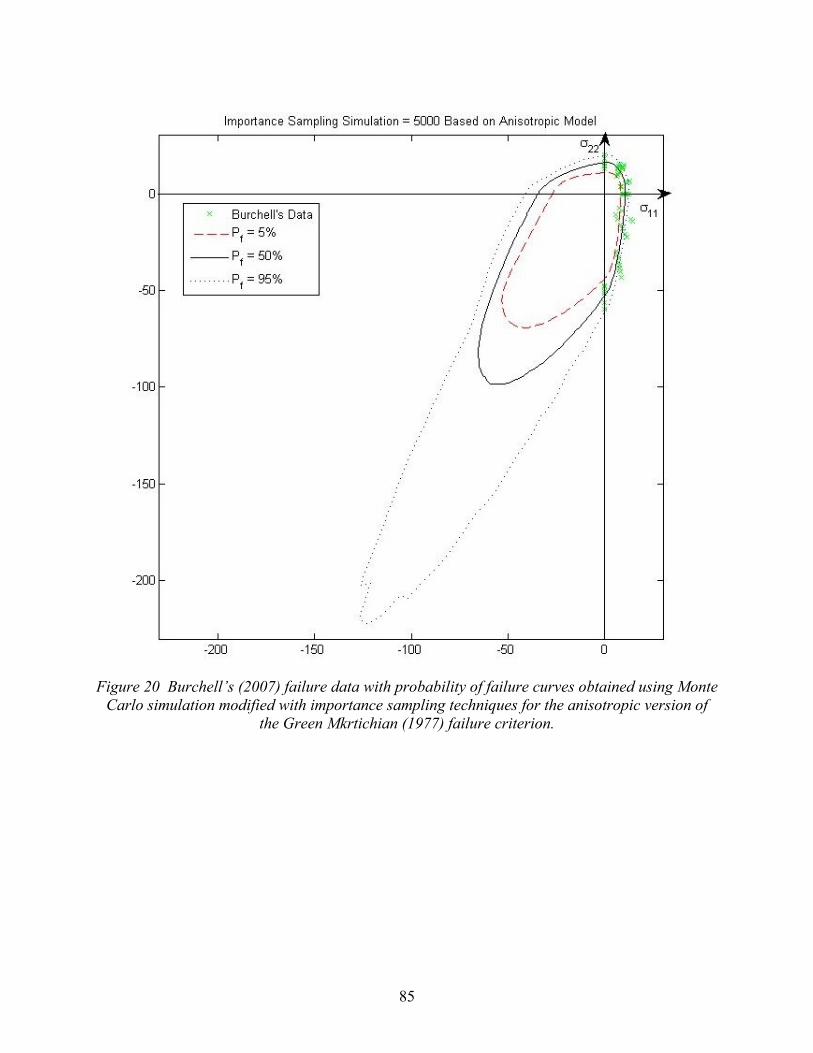
85

Figure 20 Burchell’s (2007) failure data with probability of failure curves obtained using Monte Carlo simulation modified with importance sampling techniques for the anisotropic version of

the Green Mkrtichian (1977) failure criterion.

86

IV. Codes and Standards

Measurements of material strength at failure are taken for various reasons, e.g., to conduct a comparison of the relative quality of two materials, or to establish limit loads for a given application. Relative to nuclear power generation design codes and fitness for service protocols have recognized the need to characterize the tensile strength of graphite as a random variable using an extreme value probability density functions. Characterizing the associated distribution parameters requires more data than is typically required to simply define an average value for tensile strength. The needs of experimentalists who develop test methods and nuclear design engineers who formulate design codes should dovetail on the issue of data requirements. The two parameter Weibull distribution (an extreme value distribution) has been universally adopted to characterize the random variable representing the tensile strength of nuclear graphite. Since one of the primary objectives of this project was to develop probabilistic failure models, there was motivation to develop ASTM Standard Practice D 7486 (Duffy, Baker and James, 2013). This standard outlines a procedure for estimating Weibull distribution parameters from failure data - information needed to estimate load limits for a specified level of reactor probability of failure.

Graphite failure data from bend tests or tensile tests are used to determine the Weibull modulus (m) and a Weibull characteristic strength (σθ), both of which are specific distribution parameters for the Weibull distribution. These test specimens are primarily subjected to uniaxial stress states and ASTM Standard Practice D 7486 (Duffy, Baker and James, 2013) is restricted to using only data from tensile and flexural test specimens. Hence test specimens are failed in accordance with either ASTM Standard C 565, ASTM Standard C 651, or ASTM Standard C 781. The load at which each specimen fails is recorded and the computed failure stresses are used to estimate the distribution parameters using maximum likelihood techniques. Furthermore, the standard assumes failure takes place from one unknown flaw population such that censored data techniques are not required.

The procedures appearing in ASTM Standard Practice D 7486 (Duffy, Baker and James, 2013) point to a quality assurance program for the design of components fabricated from graphite material. This quality assurance program was developed by Parikh (2011) under support from this project. One can easily generate point estimates from failure data using the maximum likelihood estimators that appear in the standard. The quality of the estimated parameters relative to the true distribution parameters depends fundamentally on the number of samples taken to failure. More information regarding the population, i.e., more failure data, always improves the quality of the point estimates of the distribution parameters. The question becomes how much data is sufficient given the application. Confidence intervals and hypothesis testing can be utilized to answer this question and at the same time assess the goodness of the estimated distribution parameters. The quality assurance program outlined in Parikh (2011) speaks directly to this issue of how good are the estimates and is currently being implemented into the ASME Boiler and Pressure Vessel Code (Section III, Division 5, Subsection HH, Subpart A Graphite Materials).

Parikh’s (2011) effort focused on a particular type of confidence bound known as likelihood confidence rings. Hypothesis testing and the relationship it maintains with parameter estimation were outlined. A test statistic was adopted that allows one to map out an acceptance region in the m - parameter distribution space. The theoretical support for the equations used

87

to generate the likelihood rings were presented. Inferential statistics allowed Parikh (1911) to generate confidence bounds on the true distribution parameters utilizing available test data. These bounds are dependent on the number of samples used to calculate point estimates. The use of inferential statistics enables the calculation of likelihood confidence rings. The concept of how the true distribution parameters lie within a likelihood ring with a specified confidence was presented in Parikh (2011). The material acceptance criterion depends on establishing an acceptable probability of failure of the component under design as well as an acceptable level of confidence associated with estimated distribution parameter. The concepts of the likelihood confidence rings and the component probability of failure curves were combined graphically providing a visual of the utility and simplicity of the method.

88

V. References

ASTM Standard C 565, “Test Methods for Tension Testing of Carbon and Graphite Mechanical Materials.”

ASTM Standard C 651, “Test Method for Flexural Strength of Manufactured Carbon and Graphite Articles Using Four-Point Loading at Room Temperature.”

ASTM Standard C 781, “Practice for Testing Graphite and Boronated Graphite Materials for High-Temperature Gas-Cooled Nuclear Reactor Components

Balzer, M.A., “Mechanical Behavior of Metals Under Triaxial Stress: Apparatus and Experiments,” Masters Thesis, University of Illinois Champaign-Urbana, 1998.

Barnett, R. L., Hermann, P.C., Wingfield, J.R., and Connors, C.L., “Fracture of Brittle Materials Under Transient Mechanical and Thermal Loading,” Report AFFDL-TR-66-220, March 1967.

Batdorf, S.B. and Crose, J.G., “A statistical Theory for the Fracture of Brittle Structure Subjected to Nonuniform Polyaxial Stress,” ASME Journal of Applied Mechanics, Vol. 41, No. 2, pp. 459-464, 1974.

Bodner, S.R. and Partom, Y., “Constitutive Equations Elastic-Viscoplastic Strain-Hardening Materials,” ASME Journal of Applied Mechanics, Vol. 42, 1975.

Boehler, J. P. and Sawczuk, A., “On Yielding of Oriented Solids,” Acta Mechanica, Vol. 27, pp. 185-204, 1977.

Boehler, J. P., Kirillov, A.A., and Onat, E.T., “On the Polynomial Invariants of the Elasticity Tensor,” Journal of Elasticity, Vol 34, pp. 97-110, 1994.

Boehler, J. P., “Yielding and Failure of Transversely Isotropic Solids, Applications of Tensor Functions in Solid Mechanics,” CISM Courses and Lectures No 292, Springer-Verlag, Berlin, pp. 3-140, 1987.

Bratton, R., private communication, 2011.

Bridgman, P.W., “The Effect of Pressure on the Tensile Properties of Several Metals and Other Materials,” Journal of Applied Physics, Vol. 24, No. 5, pp.560-570, 1953.

Burchell, T., Yahr, T. and Battiste , R., “Modeling the Multiaxial Strength of H-451 Nuclear Grade Graphite,” Carbon , Vol. 45, No. 13, pp. 2570-2583, 2007.

Cazacu, O., Cristescu, N.D., Shao, J.F., and Henry, J.P., “A New Anisotropic Failure Criterion for Transversely Isotropic Solids,” Mechanics Cohesive-Frictional Material, Vol. 3, pp. 89-103, 1998.

Cazacu, O., and Cristescu, N.D., “A Paraboloid Failure Surface For Transversely Isotropic Materials,” Mechanics of Materials, Vol. 31, No. 6, pp. 381-393, 1999.

Chaboche, J.L., “Viscoplastic Constitutive Equations for the Description of Cyclic and Anisotropic Behavior of Metals,” Bulletin De L'Academie, Ploloniase Des Science, Serie Des Science Et Techniques, Vol. 25, No. 1, pp. 33-41, 1977.

Chen, W.F., Plasticity in Reinforced Concrete, McGraw-Hill, Inc., pp. 190-250, 1982.

Chen, W.F. and Han, D.J., Plasticity for Structural Engineers, Gau Lih Book Co. Ltd., Taipei, Taiwan, 1995.

89

Chow, C.L. and Yang, F., “On One-Parameter Description of Damage State for Brittle Material,” Engineering Fracture Mechanics, Vol. 40, No. 2, pp.335-343, 1991.

Cooper, N.R., Margetson, J., and Humble, S., “Probability Of Failure Calculations And Confidence Brand Estimates For An Annular Brittle Disc Fracture Under Centrifugal Loading,” Journal of Strain Analysis for Engineering Design, Vol. 21, No. 3, 121-126, 1986.

Cooper, N. R., “Probabilistic Failure Prediction of Rocket Motor Components,” Ph.D. Dissertation, Royal Military College of Science, 1988.

Coulomb, C. A., “Essai sur une application des regles des maximis et minimis a quelquels problemesde statique relatifs, a la architecture,” Memoires de Mathematique et de Physique, presentes a l’Academie Royales Des Sciences, Vol. 7, pp. 343–387, 1776.

Drucker, D.C., and Prager, W., “Soil Mechanics And Plastic Analysis For Limit Design,” Quarterly of Applied Mathematics, Vol. 10, No. 2, pp. 157–165, 1952.

Duffy, S.F., “A Viscoplastic Constitutive Theory for Transversely Isotropic Metal Alloys,” Ph.D. Dissertation, University of Akron, 1987.

Duffy, S.F., Gyekenyesi, J.P., “Time Dependent Reliability Model Incorporating Continuum Damage Mechanics for High-Temperature Ceramics,” NASA Technical Memorandum 102046, 1989.

Duffy, S.F., and Arnold, S.M., “Noninteractive Macroscopic Reliability Model for Whisker-Reinforced Ceramic Composites,” Journal of Composite Materials, Vol. 24, No. 3, pp.235-344, 1990a.

Duffy, S.F., and Manderscheid, J.M., "Noninteractive Macroscopic Reliability Model for Ceramic Matrix Composites with Orthotropic Material Symmetry," Journal of Engineering for Gas Turbines and Power, Vol. 112, No. 4, pp. 507 511, 1990b.

Duffy, S.F., Chulya, A. and Gyekenyesi, J.P., “Structural Design Methodologies for Ceramic-Based Material Systems,” NASA Technical Memorandum 103097, 1991.

Duffy, S.F., Wetherhold, R.C. and Jain, L.K., "Extension of a Noninteractive Reliability Mod for Ceramic Matrix Composites," Journal of Engineering for Gas Turbines and Power, Vol. 115, No. 1, pp. 205 207, 1993.

Duffy, S.F., and Palko, J.L., “Analysis of Whisker Toughened CMC Structural Components Using an Interactive Reliability Model,” AIAA Journal, Vol. 32, No. 5, pp. 1043-1048, 1994.

Duffy, S.F., Baker, E.H., and James, C., "Standard Practice for Reporting Uniaxial Strength Data And Estimating Weibull Distribution Parameters For Graphite," ASTM Standard D 7846 (Passed ASTM society ballot Fall 2012).

Eason, E.D., Hall, G.N., Marsden, B.J., and Heys, G.B., “Development of a Young's Modulus Model for Gilsocarbon Graphites Irradiated in Inert Environments,” Journal of Nuclear Materials, Vol. 381, pp. 145-151, 2008.

Green, A.E. and Mkrtichian, J.Z., “Elastic Solids with Different Moduli in Tension and Compression,” Journal of Elasticity, Vol. 7, No. 4, pp. 369-386, 1977.

Greenstreet, W.L., Smith, J.E., Yahr, G.T., and Valachovic, R.S., “The Mechanical Behavior of Artificial Graphites as Portrayed by Uniaxial Tests,” Carbon, Vol. 8, No. 5, pp.649-663, 1970.

90

Griffiths, A. A., “The Theory Of Rupture And Flow In Solids,” Philosophical Transactions of the Royal Society A: Mathematical, Physical and Engineering Sciences, Vol. 221, pp. 163-198, 1921.

Gyekenyesi, J.P., “SCARE- A Post-Processor Program to MSC/NASTRAN for the Reliability Analysis of Ceramic Components,” ASME Journal of Engineering for Gas Turbines and Power, Vol. 108, No. 3, 540-546, 1986.

Harbitz, A. “An Efficient Sampling Method for Probability of Failure Calculations,” Structural Safety, Vol. 3, pp. 108-115, 1986.

Hsieh, S.S., Ting, E.C., Chen, W.F., “An Elastic-Fracture Model for Concrete,” Proceedings 3rd Engineering Mechanics Division Specialists Conference, Austin, TX, pp. 437–441, 1979.

Janosik, L.A., “A Viscoplastic Theory for Monolithic Ceramics,” Masters Thesis, Cleveland State University, 1970.

Jones, R.M. and Nelson, A.R., “Material Models for Nonlinear Deformation of Graphite,” AIAA Journal, Vol. 14, No. 6, pp. 709-717, 1976.

Lamon, J., “Reliability Analysis of Ceramics Using the CERAM Computer Program,” ASME Paper No. 90-GT-98, IGTI, 1990.

Lehknitskii, S.G., Theory of Elasticity of an Anisotropic Elastic Body, translated by P. Fern, Holden-Day Inc., San Francisco, 1963.

Li, Q.M., “Strain energy Density Failure Criterion,” International Journal of Solids and Structures, Vol. 38, No. 38, pp. 6997–7013, 2001.

Lubliner, J., Plasticity Theory, Macmillan, New York, 1990.

Mlecher, R.E., “Importance Sampling in Structural Systems, “ Structural Safety, Vol. 6, pp. 3-10, 1989

Mendelson, A., Plasticity: Theory and Application, Macmillan, New York, 1968.

Moore, S.E., “An Anisotropic Elastic-Plastic Stress Analysis of a Thick-Walled Graphite Cylinder,” Masters Thesis, The University of Tennessee. 1969.

Nova, R., and Zaninetti, A., “An Investigation Into the Tensile Behavior of a Schistose Rock,” International Journal of Rock Mechanics, Mining Sciences and Geomechanics, Vol. 27, No. 4, pp. 231-242, 1990.

Ottosen, N.S., “A Failure Criterion for Concrete,” ASCE Journal of Engineering Mechanics, Vol. 103, No. EM4, pp. 527–535, 1977.

Palko, Joseph L., “An Interactive reliability Model for Whisker- Toughened Ceramics,” Masters Thesis, June, 1992.

Parikh, A., "Quality Control Using Inferential Statistics in Weibull Analyses for Components Fabricated from Monolithic Ceramics," Masters Thesis, Cleveland State University, 2011.

Paul, B., “Generalized Pyramidal Fracture and Yield Criteria,” International Journal of Solids and Structure, Vol. 4, pp.175-196, 1968.

Rivlin, R.S. and Smith, G.F., “Orthogonal Integrity Basis for N Symmetric Matrices,” in Contributions to Mechanics, ed. D. Abir, Pergamon Press, Oxford, pp. 121-141, 1969.

91

Robinson, D.N., “A Unified Creep-Plasticity Model for Structural Metals at High Temperature,” ORNL Technical Memorandum 5986, 1978.

Saito, S., “Role of Nuclear Energy to a Future Society of Shortage of Energy Resources and Global Warming,” Journal of Nuclear Materials, Vol. 398, pp. 1-9, 2010.

Schleicher, F., “Der Spannungszustand an der Fließgrenze (Plastizitätsbedingung),” Zeitschrift für Angewandte Mathematik und Mechanik, Vol. 6, pp. 199- 216, 1926.

Seldin, E.J., “Stress-Strain Properties of Polycrystalline Graphites in Tension and Compression at Room Temperature,” Carbon, Vol. 4, No. 2, pp.177-191, 1966.

Southworth, F.H., MacDonald, P.E., Baxter, A.M., Bayless, P.D., Bolin, J.M., Gougar, H.D., LaBar, M., Moore, R.L., Ougang, A.M., Richards, M.B., Sant, R.L., Sterbentz, J.W., and Terry, W.K., “Next Generation Nuclear Power (NGNP) Project - Preliminary Assessment of Two Possible Designs,” 14th Pacific Basin Nuclear Conference, March 21-25, 2004, Honolulu, Hawaii, 2004.

Spencer, A.J.M., “Theory of Invariants,” in Continuum Physics, 1, ed. A.C. Eringen, Academic Press, London, pp. 259-353, 1971.

Spencer, A.J.M., “Continuum Theory of the Mechanics of Fibre-Reinforced Composites,” Spring-Verlag, pp.1-32, 1984.

Tabaddor, F., “A Survey of Constitutive Educations of Bimodulus Elastic Materials,” in Mechanics of Bimodulus Materials, ed: C.W. Bert, Proceedings of the American Society of Mechanical Engineering Winter Annual meeting, AMD33, 2–5 (1979).

Tresca, H., “Mémoire sur l'écoulement des corps solides soumis à de fortes pressions,” Comptes Rendus, Academie de Science, Vol. 59, p. 754, 1864.

Tsai, S.W. and Wu, E.M., “A General Theory of Strength of Anisotropic Materials,” Journal of Composite Materials, Vol. 5, pp. 58-80, 1971.

Theocaris, P.S., “The Elliptic Paraboloid Failure Criterion for Cellular Solids and Brittle Foams,” Acta Mechanica, Vol. 89, pp. 93-121, 1991.

Wetherhold, R.C. and Ucci, A.M., “Probability Techniques for Reliability Analyses of Composite Materials,” NASA CR-195294, National Aeronautics and Space Administration, National Technical Information Service, 1994.

US DOE Nuclear Energy Research Advisory Committee and the Generation IV International Forum, “A Technology Roadmap for Generation IV Nuclear Energy Systems,” GIF-002-00, December, 2002.

Vijavakumar, K. and Ashoka, J.G., “A Bilinear Constitutive Model for Isotropic Bimodulus Materials,” ASME Journal of Engineering Materials and Technology, Vol. 112, pp. 372-379, 1990.

Vijayakumar, K., and Rao, K.P., “Stress-Strain Relations for Composites with Different Stiffness in Tension and Compression,” Computational Mechanics, Vol. 2, pp. 167-175, 1987.

Von Mises, R., “Mechanik der festen Korper im plastisch deformablen Zustand,” Göttinger Nachrichten, pp. 582–592, 1913 .

92

Weibull, W., “A Statistical Distribution Function of Wide Applicability,” Journal of Applied Mechanics, Vol. 18, No. 3, pp. 293-297, 1951.

Weng, T-L, “Biaxial Fractures Strength and Mechanical Properties of Graphite-Base Refractory Composites,” ATAA Journal, Vol. 7, No. 5, pp. 850-858, 1969.

Willam, K.J. and Warnke, E.P., “Constitutive Models for the Triaxial Behavior of Concrete,” in: Proceedings of the International Association for Bridge and Structural Engineer Seminar on Structures Subjected to Triaxial Stresses (Bergamo, Italy), Vol. 19, pp. 1-31, 1974.