title pagemodified inherent strain method for predicting

Title Page

Modified Inherent Strain Method for Predicting Residual Deformation in Metal Additive

Manufacturing

by

Xuan Liang

B.S., Tsinghua University, 2011

M.S., Tsinghua University, 2015

Submitted to the Graduate Faculty of the

Swanson School of Engineering in partial fulfillment

of the requirements for the degree of

Doctor of Philosophy

University of Pittsburgh

2020

ii

Committee Page

UNIVERSITY OF PITTSBURGH

SWANSON SCHOOL OF ENGINEERING

This dissertation was presented

by

Xuan Liang

It was defended on

June 18, 2020

and approved by

Wei Xiong, Ph.D., Assistant Professor, Department of Mechanical Engineering and Materials

Science

Xiayun Zhao, Ph.D., Assistant Professor, Department of Mechanical Engineering and Materials

Science

Kevin P. Chen, Ph.D., Paul E. Lego Chair Professor, Department of Electrical and Computer

Engineering

Dissertation Director: Albert C. To, Ph.D., William Kepler Whiteford Professor, Department of

Mechanical Engineering and Materials Science

iii

Copyright © by Xuan Liang

2020

iv

Abstract

Modified Inherent Strain Method for Predicting Residual Deformation in Metal Additive

Manufacturing

Xuan Liang, Ph.D.

University of Pittsburgh, 2020

Additive manufacturing (AM) of metal components has seen rapid development in the past

decade, since arbitrarily complex geometries can be manufactured by this technology. Due to

intensive heat input in the laser-assisted AM process, large thermal strain is induced and hence

results in significant residual stress and deformation in the metal components. To achieve efficient

simulation for metal printing process, the inherent strain method (ISM) is ideal for this purpose,

but has not been well developed for metal AM parts yet.

In this dissertation, a modified inherent strain method (MISM) is proposed to estimate the

inherent strains from detailed process simulation. The obtained inherent strains are employed in a

layer-by-layer static equilibrium analysis to simulate residual distortion of the AM part efficiently.

To validate the proposed method, single-walled builds deposited by directed energy deposition

(DED) process are studied first. The MISM is demonstrated to be accurate by comparing with full-

scale detailed process simulation and experimental results.

Meanwhile, the MISM is adapted to powder bed fusion (PBF) process to enable efficient

yet accurate prediction for residual stress and deformation of large components. The proposed

method allows for calculation of inherent strains accurately based on a small-scale simulation of a

small representative volume. The extracted mean inherent strains are applied to a part-scale model

layer-by-layer to simulate accumulation of residual deformation. Accuracy of the proposed method

v

for large components is validated by comparison with experimental results, while excellent

computational efficiency is also shown.

As further applications, the MISM is extended to deal with efficient simulation for residual

deformation of thin-walled lattice support structures with different volume densities. To achieve

this goal, asymptotic homogenization is employed to obtain the homogenized inherent strains and

elastic modulus given the specific laser scanning strategy and process parameters for fabricating

those thin-walled lattice support structures. Accuracy of the homogenization-based layer-by-layer

simulation have been validated by experiments. Moreover, the enhanced layer lumping method

(ELLM) is developed to further accelerate the layer-by-layer simulation to the largest extent for

metal builds produced by PBF. By using tuned material property models, good accuracy can be

ensured while directly lumping the equivalent layers in the layer-wise simulation.

vi

Table of Contents

Preface ....................................................................................................................................... xviii

1.0 Introduction ............................................................................................................................. 1

1.1 Metal Additive Manufacturing (AM) ........................................................................... 1

1.2 Thermomechanical Simulation for Metal AM............................................................. 3

1.3 Inherent Strain Method (ISM) ...................................................................................... 5

1.4 Research Objectives ....................................................................................................... 6

1.4.1 Establishment of the MISM for DED Process ...................................................6

1.4.2 MISM Adapted to PBF Process ..........................................................................6

1.4.3 Homogenization-Based MISM for Thin-walled Lattice Structures ................7

1.4.4 Enhanced Layer Lumping Lethod (ELLM) for Simulation Accelerating ......7

2.0 Modified Inherent Strain Method (MISM) for DED Process ............................................. 9

2.1 Governing Equations of Thermomechanical Simulation ........................................... 9

2.1.1 Thermal Analysis ...............................................................................................10

2.1.2 Mechanical Analysis ..........................................................................................11

2.1.3 Element Activation Method ..............................................................................13

2.1.4 Experimental Setup for Validation of Process Modeling ...............................14

2.2 Inherent Strain Theory ................................................................................................ 15

2.2.1 Original Theory ..................................................................................................15

2.2.2 Modified Theory for AM ...................................................................................18

2.2.3 Assignment of the Modified Inherent Strain ...................................................22

2.3 Validation of the MISM ............................................................................................... 23

vii

2.3.1 Single Wall Deposition Model ...........................................................................24

2.3.2 Rectangular Contour Wall Deposition Model .................................................31

2.4 Mean Inherent Strain Vector Approach .................................................................... 38

2.5 Practical ISM based on Small-Scale Detailed Simulation ........................................ 41

2.5.1 Description of Proposed Method ......................................................................41

2.5.2 Results and Discussion .......................................................................................44

2.6 Conclusions ................................................................................................................... 46

3.0 MISM for PBF Components ................................................................................................ 49

3.1 Current Simulation Methods for PBF Components ................................................. 49

3.2 MISM Adapted for PBF Process................................................................................. 51

3.3 Calculation and Application of Inherent Strain ........................................................ 54

3.3.1 Calculation of Inherent Strain ..........................................................................54

3.3.2 Applying Inherent Strain to Part-Scale Model ...............................................61

3.4 Experimental Validation .............................................................................................. 68

3.4.1 Double Cantilever Beam ....................................................................................68

3.4.2 Canonical Part ....................................................................................................76

3.5 Conclusions and Discussions ....................................................................................... 82

4.0 Inherent Strain Homogenization for Lattice Support Structures .................................... 84

4.1 Introduction of Support Structures for PBF Process ............................................... 84

4.2 Calculation of Inherent Strains for Support Structures ........................................... 85

4.3 Asymptotic Homogenization for Lattice Structures ................................................. 91

4.4 Homogenized Material Properties .............................................................................. 97

4.4.1 RVE-Based Homogenization .............................................................................97

viii

4.4.2 Effective Mechanical Properties .....................................................................101

4.5 Experimental Validation ............................................................................................ 105

4.5.1 Simple Lattice Structured Beams ...................................................................105

4.5.2 Application to a Complex PBF Bracket .........................................................116

4.6 Conclusions and Discussions ..................................................................................... 122

5.0 Enhanced Layer Lumping Method (ELLM) for Accelerating Simulation ................... 124

5.1 Current State of Simulation for PBF ........................................................................ 124

5.2 Enhanced Layer Lumping Method (ELLM) ........................................................... 126

5.2.1 Layer Activation Thickness (LAT) Effect .....................................................126

5.2.2 Meso-Scale Modeling of Residual Stress Evolution ......................................133

5.3 Validation Examples for ELLM................................................................................ 141

5.3.1 2-Layer ELLM .................................................................................................144

5.3.2 3-Layer ELLM .................................................................................................146

5.3.3 4-Layer ELLM .................................................................................................148

5.3.4 Discussions ........................................................................................................151

5.4 Conclusions ................................................................................................................. 154

6.0 Conclusions .......................................................................................................................... 156

6.1 Main Contributions .................................................................................................... 156

6.2 Future Works .............................................................................................................. 159

Bibliography .............................................................................................................................. 162

ix

List of Tables

Table 2.1 Geometrical Parameters of the LENS Depositions ................................................. 24

Table 2.2 Maximum Vertical Residual Distortion of the Part after LENS Deposition of a

Straight Line and Computational Times by Detailed Process Simulation and Conventional

ISM ........................................................................................................................................... 27

Table 2.3 Maximum Vertical Residual Distortion of the Part with Line Depositions and

Computational Times by Detailed Process Simulation and MISM.................................... 30

Table 2.4 Geometrical Parameters of the LENS Rectangular Contour Depositions ........... 33

Table 2.5 Maximum Vertical Residual Distortion of the Part with Rectangular Contour

Deposition and Computational Times by the Detailed Process Simulation and the MISM

................................................................................................................................................... 34

Table 2.6 Vertical Residual Distortion (Unit: mm) of the Substrate with a LENS Deposited

5-Layer Rectangular Contour in Three Different Ways ..................................................... 38

Table 2.7 Maximum Vertical Residual Distortion of the Substrate with LENS Deposited 3-

and 5-Layer Straight Wall Structure and Computational Times by Detailed Process

Simulation and Layered ISM ................................................................................................. 40

Table 2.8 Maximum Vertical Deformation of the Rectangular Contour Deposition Model

Using Full-Scale Process Simulation and the MISM based on Small-Scale Process

Simulation ................................................................................................................................ 44

Table 2.9 Comparison of Detailed Process Simulation and the MISM in Terms of

Computational Efforts Required for the 5-Layer and 10-Layer Rectangular Contour

Deposition Model .................................................................................................................... 46

x

Table 3.1 Default DMLS Process Parameters of the Core-Skin Mode for Ti64 and Inconel

718............................................................................................................................................. 55

Table 3.2 Comparison of the Residual Total Deformation in the Simulated and Experimental

Results ...................................................................................................................................... 71

Table 3.3 Computational Time of the Layer-by-Layer Simulation for the Double Cantilever

Beam Having Different Number of Equivalent Layers ....................................................... 72

Table 4.1 Volume Densities of the Thin-Walled Lattice Support Structures with Changing

Space Size ................................................................................................................................. 98

Table 4.2 Homogenized CTEs for the Thin-Walled Lattice Support Structures of Different

Volume Densities ................................................................................................................... 100

Table 4.3 Yield Strength of the Thin-Walled Lattice Support Structures of Different Volume

Densities ................................................................................................................................. 105

Table 5.1 Computational Time of Five Simulation Cases for Short Cantilever Beam....... 129

Table 5.2 MPMs for IN718 Used in the ELLM Implementation ......................................... 141

Table 5.3 Computational Time of the Five Simulation Cases for Large Cantilever Beam 151

Table 5.4 Maximum Displacement before (BSR) and after Support Removal (ASR) for the

Large Cantilever Beam......................................................................................................... 152

xi

List of Figures

Figure 1.1 Typical Schematic Diagram of PBF Drocess Using Laser Heat Source [4] .......... 2

Figure 1.2 Successful Repair Case Studies Using the (a) Optomec LENS System: (b) Inconel

718 Compressor Seal [18] ......................................................................................................... 3

Figure 2.1 The Optomec LENS 450 Metal Printer .................................................................. 14

Figure 2.2 Experimental Setup: (a) the Fixture and Substrate (b) the 3D Laser Scanning

Device ....................................................................................................................................... 15

Figure 2.3 Original Definition of Inherent Strain for Welding Mechanics ........................... 16

Figure 2.4 Schematic Illustration of Mechanical Strain Induced at a Material Point during a

Simple Welding Process ......................................................................................................... 19

Figure 2.5 Two States for the First Layer of a 2-Layer Deposition: (a) Depositing Starts from

Right Side; (b) Mechanical Boundary for the Concerned Material Points (Red Circle) Is

Considered as Stable after the First Layer Is Deposited; (c) The Entire Part Reaches the

Final Steady State ................................................................................................................... 20

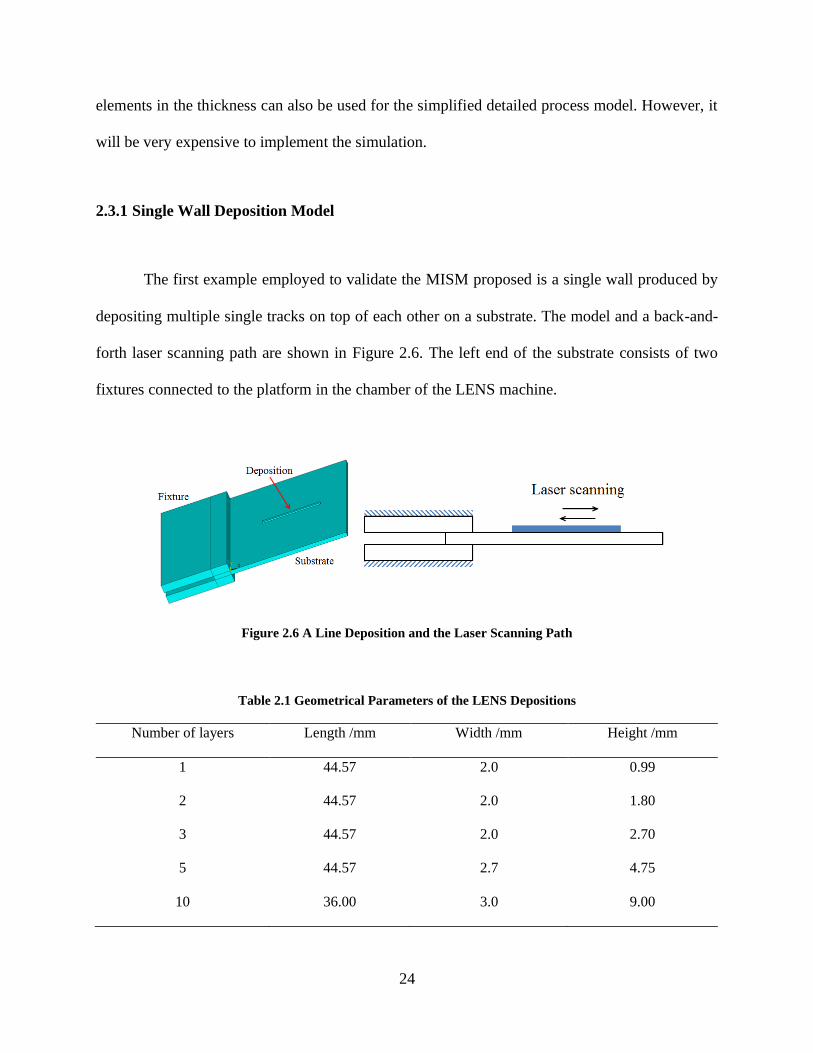
Figure 2.6 A Line Deposition and the Laser Scanning Path ................................................... 24

Figure 2.7 Vertical Residual Distortion (Unit: m) of a 1-Layer Line Deposition by Detailed

Process Simulation .................................................................................................................. 26

Figure 2.8 The Extracted Elemental Inherent Strains of the Lower Layer in a 2-Layer Line

Deposition ................................................................................................................................ 28

Figure 2.9 Vertical Residual Distortion (Unit: m) of the 1-Layer Line Deposition by the

MISM ....................................................................................................................................... 29

xii

Figure 2.10 Vertical Residual Distortion (Unit: m) of the 5-Layer Line Deposition by (a) the

Detailed Process Simulation and (b) the MISM ................................................................... 31

Figure 2.11 Laser Scanning Path of the Rectangular Contour Deposition ........................... 32

Figure 2.12 Illustration of the Geometry of the Rectangular Contour Deposition ............... 33

Figure 2.13 Vertical Residual Distortion (Unit: m) of the Part with the 2-Layer Contour

Deposition (a) by the Detail Process Simulation and (b) by the MISM ............................. 35

Figure 2.14 Vertical Residual Distortion (Unit: m) of the Part with the 5-Layer Contour

Deposition (a) by Detailed Process Simulation and (b) by the MISM ............................... 35

Figure 2.15 The Experimental Setup and the 5-Layer Contour Deposition by LENS ......... 36

Figure 2.16 Vertical Residual Distortion (Unit: mm) of the Substrate with LENS Deposition

of 5-Layer Rectangular Contour by (a) MISM (b) Detailed Process Simulation (c)

Experimental Measurement ................................................................................................... 37

Figure 2.17 Typical Features of the Small-Scale Model: (a) Geometry and Mesh Model and

(b) Stabilized Temperature Contour in a Deposition Layer ............................................... 42

Figure 2.18 Predicted Distribution of Vertical Residual Deformation (Unit: m) of the 10-

Layer Rectangular Contour Deposition by (a) Full-Scale Process Simulation (b) Mean

Inherent Strain Vector Method ............................................................................................. 45

Figure 3.1 Small-Scale Model: (a) a 2-Layer Representative Volume on the Bottom-Fixed

Substrate and the Laser Scanning Strategy, and (b) Illustration of the Intermediate and

Steady State of a Ti64 Material Point (Black Dot)............................................................... 57

Figure 3.2 2-Layer Example for Illustration of the Layer-by-Layer Method of Assigning

Inherent Strain ........................................................................................................................ 63

Figure 3.3 Workflow of the MISM-Based Simulation for Metal AM Process ...................... 67

xiii

Figure 3.4 Double Cantilever Beam: (a) Geometry Profile; (b) Ti64 Deposition before and

after Cutting off the Support Structures (Similar Phenomenon Also Observed in the Case

of Inconel 718); (c) Finite Element Mesh of the Beam and the Substrate with the Bottom

Surface Clamped ..................................................................................................................... 69

Figure 3.5 Maximum Total Deformation of Point 1 and 2 after Stress Relaxation of the

Double Cantilever Beam Containing Varying Number of Equivalent Layers, through the

Experiment and ISM .............................................................................................................. 73

Figure 3.6 The Differences between the Predicted and Experimental Results in Point 1 and

2 Changing with the Number of Lumped Physical Layers in One Equivalent Layer ...... 76

Figure 3.7 A Complex Canonical Part Utilized to Validate the Proposed Method: Geometry

Profile and Meshed Model Including the Substrate Using All Tetrahedral Elements ..... 77

Figure 3.8 Two Sample Lines in the Meshed Model and the Printed Component by DMLS

in Ti64 ...................................................................................................................................... 78

Figure 3.9 Residual Displacements Perpendicular to the Outer Surface on (a) Sample Line 1

and (b) Sample Line 2 Obtained by the Modified Method, the Original Method and

Experimental Measurement ................................................................................................... 79

Figure 4.1 Thin-Walled Lattice Support Structures for Overhang Features in the Inconel

718 Component........................................................................................................................ 85

Figure 4.2 Thin-Walled Support Structure: (a) the Representative Volume for Small-Scale

Modeling and (b) the Laser Scanning Strategy and Space Size (in mm) ........................... 87

Figure 4.3 Distribution of the Normal Inherent Strains in a Single Wall of the Lattice

Support Structures.................................................................................................................. 88

xiv

Figure 4.4 Thin-Walled Support Structures in the DMLS Process: (a) Inconel 718 Lattice

Depositions; (b) the CAD Model of a Thin-Walled Lattice Block; (c) the Representative

Unit Cell (Red Dashed Square) .............................................................................................. 91

Figure 4.5 The RVE Model and Directional Inherent Strains for Thin-Walled Lattice

Support Structures.................................................................................................................. 99

Figure 4.6 Tensile Specimens of Thin-Walled Lattice Structures Fabricated (a) Horizontally

and (b) Vertically by DMLS................................................................................................. 102

Figure 4.7 Experiment Setup of the Standard Tensile Tests ................................................ 102

Figure 4.8 Experimental Loading Force-Displacement Curves for Horizontal (HOR) and

Vertical Specimens (VER) of Different Volume Densities by the Tensile Tests ............. 103

Figure 4.9 Homogenized and Experimentally Measured Elastic Modulus of the Thin-Walled

Lattice Support Structures................................................................................................... 104

Figure 4.10 Four Beam Samples by DMLS: (a) As-Built Lattice Support Structures on a

Solid Base; (b) Varying Space Sizes for Different Volume Densities ............................... 106

Figure 4.11 Lattice Structure Beams after Stress Release: (a) the Cutting-off Interface and

(b) Vertical Deformation ...................................................................................................... 107

Figure 4.12 The Full-Scale Model of the Lattice Structure Block with 1.0 mm Space Size108

Figure 4.13 The Half-Size Model under Symmetrical Constraint Condition: (a) Detailed

Thin-Walled Lattice Structures; (b) Homogenized Solid Model ...................................... 110

Figure 4.14 Vertical Residual Deformation (Unit: mm) for Volume Density of 0.19 through

(a) Half-Size Detailed Modeling, (b) Half-Size Homogenization-Based Modeling and (c)

Experimental Measurement ................................................................................................. 111

xv

Figure 4.15 The Vertical Residual Deformation for Different Volume Densities Obtained by

(a)~(c) the Half-Size Homogenization-Based Modeling and (d)~(f) the Experimental

Measurement ......................................................................................................................... 112

Figure 4.16 Vertical Residual Deformation along the Top Center Line of the Beam with

Different Volume Densities .................................................................................................. 114

Figure 4.17 Area Integral Values for Residual Deformation Curves for Overall Error

Evaluation .............................................................................................................................. 116

Figure 4.18 Geometrical Dimensions of a Complex Bracket with Thin-Walled Support

Structures............................................................................................................................... 117

Figure 4.19 Tetrahedron Element Mesh for the Complex Component with Homogenized

Support Structures................................................................................................................ 118

Figure 4.20 L-BPF Component with Thin-Walled Support Structures before and after

Cutting Process...................................................................................................................... 119

Figure 4.21 Residual Deformation Comparison of the Bracket with Support Structures after

Cutting Process through (a) Simulation (Vertical Displacement) and (b) Experimental

Measurement (Surface Normal Deformation) ................................................................... 120

Figure 5.1 The Short Cantilever Beam as The Benchmark Case: (a) Geometrical Profile; (b)

Finite Element Mesh and Boundary Condition for the Half Model ................................ 127

Figure 5.2 The PBF Short Cantilever Beam Samples (a) before and (b) after Support

Removal by W-EDM............................................................................................................. 128

Figure 5.3 Vertical Residual Deformation along Center Line of the Top Surface of the Short

Cantilever Beam Obtained by Five Simulation Cases and Experiment .......................... 130

xvi

Figure 5.4 Residual Deformation of the 2 mm Tall Cantilever Beam Obtained by the (a) 5L5S

Case and (b) Experiment ...................................................................................................... 132

Figure 5.5 The Meso-Scale 10-Layer Block Model with Fixed Bottom Surface ................. 133

Figure 5.6 Directional Residual Stress Distribution in the Core Area of the 4th Layer in the

(a) Activation and (b) Following-Activation Step .............................................................. 134

Figure 5.7 Stress Relaxation Effect on the 4th Layer due to Addition of the Upper Layer in

the Meso-Scale Modeling ...................................................................................................... 135

Figure 5.8 Positions of the Concerned Points in the 4th Layer for Stress Evolution

Observation ........................................................................................................................... 136

Figure 5.9 Directional Stress Evolution History of Three Sample Points in the 4th Layer 136

Figure 5.10 Directional (a) Elastic and (b) Plastic Strain Evolution History of Three Material

Points in the Meso-Scale Model ........................................................................................... 137

Figure 5.11 Typical Directional Strain Evolution History for a Material Point in Bulk

Volume of the Meso-Scale Model ........................................................................................ 138

Figure 5.12 Residual Stress Evolution and Equivalent Material Models due to 2-Layer and

3-Layer Lumping .................................................................................................................. 140

Figure 5.13 Geometrical Profile and Finite Element Mesh of the Large Cantilever Beam 142

Figure 5.14 Residual Deformation in the (a) Longitudinal and (b) Vertical Build Direction

before (BSR) and after Support Removal (ASR) Simulated Using 32 Load Steps

(Benchmark No-Lumping Case) .......................................................................................... 143

Figure 5.15 Vertical Deformation along Center Line of the Top Surface of the Cantilever

Beam after Support Removal Obtained by the No-Lumping Simulation and Experiment

................................................................................................................................................. 144

xvii

Figure 5.16 Division of the Equivalent Layers in the Cantilever Beam Ready for Assignment

of Two MPMs ........................................................................................................................ 145

Figure 5.17 The (a) Longitudinal and (b) Vertical Residual Deformation before (BSR) and

after Support Removal (ASR) Using 2-Layer ELLM Involving One Tuned MPM ....... 145

Figure 5.18 Vertical Residual Deformation after Support Removal (ASR) Using 2-Layer

LLM without Tuned MPM .................................................................................................. 146


after Support Removal (ASR) Using 3-Layer ELLM with Two Tuned MPMs .............. 147


after Support Removal (ASR) Using 4-Layer ELLM with Three Tuned MPMs ........... 148

Figure 5.21 Two-Section Division (TSD) of the Cantilever Beam for the 4-Layer ELLM Case

................................................................................................................................................. 150


after Support Removal (ASR) Using 4-Layer ELLM in Combination with Two-Section

Division (TSD) ....................................................................................................................... 150

Figure 5.23 Comparison of the Vertical Deformation (ASR) along the Top Surface Center

Line of the Cantilever Beam Obtained in No-Lumping and Different ELLM Cases ... 153

xviii

Preface

Five years ago, when I first arrived at the University of Pittsburgh, I never expected the

experience of pursuing my doctoral degree would be so unforgettable. I feel very lucky to reach

the end of my study successfully. I would like to thank many people who give generous support

to me in the completion of this dissertation.

First, I would like to give my sincere gratitude to my advisor, Prof. Albert C. To for his

insightful guidance and full support for the completion of my dissertation. I got a lot of benefit

from the discussions with Prof. To in the past years. Moreover, He encouraged me to attend many

academic conferences to practice my presenting and communicating skills. These experiences are

extremely unforgettable in my life.

Second, I would like to say sincere thanks to my committee members, Prof. Wei Xiong,

Prof. Xiayun Zhao, and Prof. Kevin P. Chen, for their serving on my committee regardless of a

tight time schedule. They gave a lot of insightful comments on my research work. Their valuable

suggestions have greatly improved the quality of my dissertation.

Third, I also would like to thank my colleagues in the computational mechanics group for

their kind collaboration and patient help. I would like to give my gratitude to many past and current

members: Dr. Pu Zhang, Dr. Qingcheng Yang, Lin Cheng, Qian Chen, Wen Dong, Hao Deng,

Shawn Hinnebusch, Dr. Hai T. Tran, and among others, for generous sharing of their expertise. I

also want to thank Ran Zou and Shuo Li in Prof. Kevin P. Chen’s group for their nice collaboration.

Moreover, I would like to thank Brandon Blasko and Andrew Holmes in the Swanson Center for

Product Innovation of University of Pittsburgh for their help in the experiments.

xix

In particular, I would like to give acknowledgement to funding support from Army SBIR,

and technical support from commercial companies including ANSYS, Materials Science

Corporation (MSC) and Oberg Industry, etc. Specifically, I would like to thank my collaborators,

Jason Oskin and John Lemon from Oberg Inc., for their help in some of the experiments involved

in this dissertation.

At last, I want to owe my deepest and sincere gratitude to my wife and my parents. Without

their endless support and encouragement, it would not be possible for me to stick to the end and

complete my dissertation. Your love and support give me the largest power and help me move

forward with courage in my life.

1

1.0 Introduction

The primary goal of this dissertation is to propose an efficient simulation method that can

predict residual stress and deformation of large metal components fabricated by the AM process.

The main focus of the simulation method lies in the thermal and mechanical analysis involving

elastic and elastoplastic mechanics. As a further application, efficient simulation of thin-walled

metal lattice structures is also studied in order to show the excellent performance and large

potential of the proposed method in real practice. The motivation, background and research

objective are presented in this chapter.

1.1 Metal Additive Manufacturing (AM)

Restricted by its subtractive nature, it is difficult to employ machining techniques to

produce metal parts with complex geometries, especially those with internal features. However,

the demand for complex-shaped parts has increased rapidly since metal parts consisted of

microscopic structures (e.g. cellular structures) have been shown to have excellent mechanical

performance under certain conditions [1, 2]. Therefore, additive manufacturing (AM) has received

much interest lately and is considered an important technique for fabricating complex-shaped

workpieces [3, 4]. In modern AM processes, the CAD model of a part is sliced into many thin

layers, where each layer is “printed” successively in a bottom-up manner [5-10]. In this way, any

complex geometry can be produced by AM. For example, AM has been employed to print complex

structures [2, 11] designed by topology optimization [11-16].

2

On the one hand, powder bed fusion (PBF) process is currently the most popular AM

process for manufacturing complex metal components. For example, selective laser melting

(SLM), direct metal laser sintering (DMLS) and electron beam melting (EBM) are powder bed

based. A metal part is sliced into planar layers and then built from bottom up in a powder bed.

Thin layers of metal powder are spread over a clamped build plate by a moving roller or spreader

as shown in Figure 1.1. Each thin layer is fused by laser or electric beam via a micro-welding

process [17] in a pass-by-pass manner following the prescribed scan paths and patterns. Metal

powder fusion only occurs in those areas where a raster motion of the laser or electric beam heat

source involves. Rapid melting and solidification of metal powders occurs in the scan tracks,

forming the final metal components.

Figure 1.1 Typical Schematic Diagram of PBF Drocess Using Laser Heat Source [4]

On the other hand, directed energy deposition (DED) is the other category of metal AM

processes. It is more suitable for making repairs, adding features to an existing component, or even

3

making parts with different materials during the same build. A representative DED process is the

LENS (Laser Engineered Net Shaping) [18-20], which is based on feeding powder into the melt

pool created by a high energy laser beam. Figure 1.1 illustrates an example stemming from the use

of LENS that will be employed in this dissertation.

(a) (b)

Figure 1.2 Successful Repair Case Studies Using the (a) Optomec LENS System: (b) Inconel 718 Compressor

Seal [18]

1.2 Thermomechanical Simulation for Metal AM

At the macroscopic scale, different metal AM processes that employ a high-energy heating

source are generally based on similar physical processes involving melting and solidification of

metal. Hence in a typical metal AM process, large temperature gradient and high cooling rate

occurs due to intensive heat input and large local energy density, which consequently lead to large

thermal strains and residual stress or distortion in an AM metal part [21-23].

4

Unless post stress relief is performed, removal of substrate or support structures after

printing would result in further deformation of the AM part and residual stress and strain would

redistribute [24]. In order to predict the residual distortion and stress introduced into the part by an

AM process, since the physical process of AM has some commonalities with the metal welding

phenomenon, some simulation methods focused on the metal welding problem have been extended

for metal AM processes [25-29]. Numerical approaches employing the finite element analysis

(FEA) have been implemented [29-33]. Based on the simulations, optimization of laser scanning

strategies, build-up directions, or design of support structures could be further investigated [34].

Part-scale AM process simulation to compute residual stress and distortion is very time-

consuming since it is a long time-scale problem involving transient heat transfer, non-linear

mechanical deformation, and addition of large amount of materials [27-29]. Depending on the

material under consideration, either a fully coupled or decoupled thermomechanical analysis can

be employed. For example, in a decoupled analysis, the thermal analysis is first performed to

acquire the temperature distribution at each time step, followed by assigning the obtained thermal

load as temperature field at the corresponding step in the mechanical analysis [35, 36]. Obviously,

the entire process simulation becomes increasingly time-consuming as large amount of materials

are being deposited, and as a result, the size of the modeled part or the number of depositing layers

is severely limited. The required simulation time ranges from several hours to days, or even weeks.

In order to enable practical AM process simulation, the simulation time must be reduced radically.

5

1.3 Inherent Strain Method (ISM)

Decades ago, the inherent strain method (ISM) [37-41] was developed and established to

enable fast estimation of residual distortion/stress in metal welding. Both simulation and

experimental results validate the accuracy and efficiency of the ISM for predicting residual

distortion/stress of simple metal welding. Another computationally efficient method inspired by

the inherent strain theory is the method of applied plastic strain [42, 43]. It utilizes 2D elastoplastic

simulation to calculate the plastic strain and then apply it as an equivalent mechanical load to the

3D model to evaluate residual distortion/stress. Both the inherent strain and applied plastic strain

method are capable of significantly reducing the computational cost of the thermomechanical

simulation [43, 44]. However, the physical process of AM is much more complicated compared

with simple metal welding. Attempts to directly apply the inherent strain or the applied plastic

strain method to the AM process have failed to obtain accurate residual distortion or stress of builds

with multiple deposition layers. In recent years, some other approaches based on the inherent strain

theory have been developed, and the computed inherent strain is imposed onto a macro-scale

model to obtain mechanical deformation [45-47]. This method is easy to implement and

computationally fast, but it is a challenge to achieve good accuracy in predicting residual distortion

at part scale [48].

6

1.4 Research Objectives

1.4.1 Establishment of the MISM for DED Process

Detailed thermomechanical simulation of powder-fed LENS process is numerically

implemented and validated first as the basic knowledge for AM process. Then the MISM is

proposed to estimate the inherent strains accurately from detailed AM process simulation for fast

residual distortion simulation of single-walled structures produced by the representative DED

process in LENS. These singled-walled structures considered here are composed of laser scan lines

deposited on top of each other but not on their sides, except at the connections where two walls

join with each other. Obviously, the purpose of considering only these geometrically simple

structures is to simplify the problem and model formulation for fast residual distortion prediction.

A challenge of doing the same for complex-topological structures is expected to build on top of

the model proposed in this dissertation. As a natural extension, the concept of mean inherent strain

vector will be proposed which will be extracted from the two-layer and three-layer line deposition

models. Numerical examples will demonstrate the mean inherent strain can be applied to simple

wall depositions containing more layers to accurately predict residual deformation much faster. A

small-scale simulation model is further proposed to extract the mean inherent strain for applying

to different single-walled DED parts and predicting residual deformation efficiently.

1.4.2 MISM Adapted to PBF Process

The MISM will be adapted to the PBF DMLS process and employed to predict the residual

distortion of the large and complex metal components efficiently. The MISM will be adapted

7

carefully to the specific physical phenomena in the DMLS process. The detailed procedure of

extracting the inherent strain based on small-scale thermomechanical simulation will be

demonstrated. Also, the way that the mean inherent strain vector is obtained and assigned to

different large-scale builds will be explained. Numerical examples will be provided to validate the

proposed method by comparing its prediction with experimental measurement of DMLS double

cantilever beam and the complex canonical component. Computational efficiency of the proposed

method will also be shown.

1.4.3 Homogenization-Based MISM for Thin-walled Lattice Structures

The effective inherent strains for thin-walled lattice support structures will be figured out

based on asymptotic homogenization given the specific process parameter and laser scanning

strategy. Meanwhile, the effective mechanical property like elastic modulus of the lattice support

structured of different volume densities will also be obtained. The homogenized inherent strains

and mechanical properties will be fully employed to enable efficient analysis in the layer-by-layer

simulation for large components with support structures. This novel idea will adapt the proposed

MISM to more scenarios such as other types of lattice support structures involved in the PBF

fabricating process.

1.4.4 Enhanced Layer Lumping Lethod (ELLM) for Simulation Accelerating

The enhanced layer lumping method (ELLM) is developed in order to accelerate the layer-

wise simulation to the largest extent, while ensuring good simulation prediction at the same time

for the large metal components produced by PBF. The residual stress/strain evolution history due

8

to layer-wise material addition in the meso-scale modeling. Considering the observed evolution

feature, tuned material property models (MPMs) are proposed to control the stress level when

many equivalent layers are activated and deformed simultaneously in the layer-by-layer

simulation. The simulation results obtained through the ELLM with tuned MPMs are validated by

comparison to experimental results. The computational times for different ELLM cases are also

shown, which indicates the greatly accelerated simulation by the proposed method.

9

2.0 Modified Inherent Strain Method (MISM) for DED Process

2.1 Governing Equations of Thermomechanical Simulation

Since the inherent strains have to be extracted based on the history of mechanical strain, a

detailed thermomechanical simulation for the metal AM has been fully developed, and the key

governing equations are briefly reviewed below. In order to ensure accuracy of the extracted

inherent strains, the detailed process model has to satisfy a few characteristics. For example, it

should be able to capture the exact peak temperature of any concerned material point in the AM

process, since it will influence the mechanical strains of the intermediate state. Therefore, a

reasonable heat source model should be employed to capture the shape of the melt pool.

Meanwhile, sufficient number of load steps should be used to simulate the detailed laser scanning

path. Otherwise, the temperature distribution, especially the far-field temperature, obtained by the

thermal analysis may not match the experimental measurement. Moreover, the effects of the

evolving mechanical boundaries on the inherent strains extracted cannot be fully considered

without enough simulation steps. The number of load steps should be determined based on element

size and physical parameters of the heat source such as the laser penetration depth. New elements

in each thin layer are activated in each load step to simulate the material depositing process. Some

elements are possibly not activated if coarse load steps are employed in the detailed process

simulation. To avoid this problem, the number of load steps is first estimated roughly by dividing

the deposition layer length by the radius of the laser beam. Then denser load steps have to be

employed to ensure that all the elements in a layer will be activated step by step. This is general

10

rule for considering the least number of load steps are needed to ensure good accuracy for the

detailed process model.

2.1.1 Thermal Analysis

Assume a Lagrangian frame Ω and a material point located by 𝒓(𝒓 ∈ Ω) as the reference.

Given thermal energy balance at time 𝑡, the governing equation can be formulated as follows [36]:

𝜌𝐶𝑝𝑑𝑇(𝒓,𝑡)

𝑑𝑡= −∇ ∙ 𝒒(𝒓, 𝑡) + 𝑄(𝒓, 𝑡), 𝒓 ∈ Ω (2.1)

where 𝜌 denotes the material density; 𝐶𝑝 denotes the specific heat capacity; T denotes the

temperature field; 𝒒 denotes the thermal flux vector and 𝑄 denotes the internal heat source.

Expression of the thermal flux vector 𝒒 can be written as:

𝒒 = −𝑘∇𝑇 (2.2)

where k is the thermal conductivity coefficient and ∇𝑇 indicates the temperature change. Material

properties such as thermal conductivity coefficient and specific heat capacity are usually

temperature dependent.

The internal heat source 𝑄 exerts a significant influence on the thermal modeling of the

AM process, since the heat input is the fundamental cause of the residual distortion and stress.

Different mathematical models have been proposed in the literature [49-52] to construct equations

of the heat source. The difference between those models is generally different number of degrees

of freedom. Among the heat source models, the double ellipsoidal model [53] has been widely

used [33, 35, 54-56], which may be the most sophisticated model proposed so far. The pattern of

the heat generation rate is assumed to be Gaussian. However, those equations are generally

proposed under a specific condition and should be modified to match the actual size of the melt

11

pool. Acceptable ways for comparing parameter fitting of the heat source model in order to match

the geometry in the micrograph can be found in the references [55, 56].

For the thermal analysis, the initial condition regarding the temperature is assigned as

follows:

𝑇(𝒓, 0) = 𝑇0(𝒓, 0), 𝒓 ∈ Ω (2.3)

Equations corresponding to different types of thermal boundary conditions in the AM

process are generally classified into three categories:

𝑇 = �̅�, 𝒓 ∈ Γ𝐷𝑇 (2.4)

−𝑘∇𝑇 ∙ 𝒏 = 𝑞,̅ 𝒓 ∈ Γ𝑁𝑇 (2.5)

−𝑘∇𝑇 ∙ 𝒏 = ℎ(𝑇 − 𝑇𝑎), 𝒓 ∈ Γ𝑅𝑇 (2.6)

Equation (2.4) gives the Dirichlet boundary condition on the boundary Γ𝐷𝑇 where the

temperature field is prescribed as �̅�. Equation (2.5) gives the Neumann boundary condition on the

boundary Γ𝑁𝑇, whereas the heat flux is defined with the normal vector 𝒏 to Γ𝑁

𝑇; Equation (2.6) shows

the Robin boundary condition where the surface heat convection with the convection coefficient h

between the ambient temperature Ta and the surface temperature T is applied on Γ𝑅𝑇. There is no

overlap among Γ𝐷𝑇, Γ𝑁

𝑇and Γ𝑅𝑇 and Γ𝐷

𝑇 ∪ Γ𝑁𝑇 ∪ Γ𝑅

𝑇 = 𝜕Ω𝑇.

2.1.2 Mechanical Analysis

Quasi-static mechanical analysis is generally implemented to calculate the mechanical

response such as the residual distortion and stress for AM builds. The temperature history obtained

by the abovementioned thermal analysis is applied to the model as an external load and boundary

12

constraint. The governing equation corresponding to the quasi-static mechanical analysis can be

written as follows:

∇ ∙ 𝝈 + 𝒃 = 𝟎, 𝒓 ∈ Ω (2.7)

where 𝝈 denotes the stress tensor and 𝒃 represents the body force vector of the model. As for the

boundary conditions, the Dirichlet and Neumann boundary conditions will be considered, as

formulated in Eqs. (2.8) and (2.9) in the following:

𝒖 = �̅�, 𝒓 ∈ Γ𝐷𝑀 (2.8)

𝝈 ∙ 𝒏 = �̅�, 𝒓 ∈ Γ𝑁𝑀 (2.9)

where u denotes the displacement vector and is prescribed �̅� on the mechanical boundary Γ𝐷𝑀. In

Eq. (2.9), dot product of the stress tensor 𝝈 and normal vector 𝒏 is the surface traction vector,

which is prescribed �̅� on the mechanical boundary Γ𝑁𝑀.

In this dissertation, the temperature dependent elastic-plastic material model is utilized in

order to be better consistent with practical mechanical behavior of metal materials in the AM

process. The constitutive equation of the material model can be written as follows:

𝜎𝑖𝑗 = 𝐶𝑖𝑗𝑘𝑙(𝐸𝑘𝑙 − 𝐸𝑘𝑙𝑝 − 𝐸𝑘𝑙

𝑡ℎ) (2.10)

where 𝐶𝑖𝑗𝑘𝑙 denotes the fourth-order tensor of elasticity; 𝐸𝑘𝑙, 𝐸𝑘𝑙𝑝

, and 𝐸𝑘𝑙𝑡ℎ represent the total,

plastic and thermal strain, respectively. The associate J2 plasticity model with temperature-

dependent mechanical properties is used in the analysis. The details of the process model can be

found in Ref. [55].

13

2.1.3 Element Activation Method

In an AM process, materials are deposited in a layer-by-layer manner. The elements in each

of the deposited layers do not have any contribution to the FEA until the heat source arrives. As

the heat source moves sufficiently close, the elements surrounding the laser spot will be deposited.

When the deposition ends, all the elements involved in the deposition are activated and contribute

to the thermal and mechanical analysis. For this purpose, the birth and death element activation

method [35, 55, 57] is utilized in this dissertation. Advantages of the birth and death element

technique include the following two aspects. On the one hand, no ill-conditioning problem will be

introduced to the matrix of structural global stiffness and mass. On the other hand, only the degrees

of freedom of active elements are involved, which contributes to a relatively small algebraic

system to solve.

Nevertheless, the element birth and death technique has the following disadvantages. First,

it is not easy to implement the method into the commercial FEA software through user-defined

subroutines. Second, renumbering of the equations and re-initialization of the solver are performed

every time new elements are activated, which will negate savings of the computational cost.

In addition, an element activation criterion is required to determine whether an element

needs to be activated in the simulation. A feasible activation criterion combined with the double

ellipsoid heat source model is employed in this dissertation. The inactive elements are activated

where the heat power is higher than 5% of the maximum value at the ellipsoid center [55].

14

2.1.4 Experimental Setup for Validation of Process Modeling

The LENS 450 metal AM system (Optomec, Albuquerque, NM) used to perform the

experiment is shown in Figure 2.1, and the material being printed is a titanium alloy called Ti-6Al-

4V (Ti64).

Figure 2.1 The Optomec LENS 450 Metal Printer

A fixture that mounts onto the build platform is designed to hold a small substrate for

deposition, which acts as a cantilever that allows residual deformation to be measured (see Figure

2.2(a)). The LENS system allows the input of the exact build path and process parameters such as

the laser power, scanning velocity, and powder feed rate. After printing is completed, 3D laser

scanning device shown in Figure 2.2(b) is utilized to measure the residual distortion of the part in

the vertical direction. Before measuring the residual distortion, a calibration test against the laser

scanning device should be performed first. Difference between two scanned configurations of an

identical part is taken as the system error of the measurement. It suggests that the measurement

error of the 3D laser scanning device is ±0.075 mm.

15

(a) (b)

Figure 2.2 Experimental Setup: (a) the Fixture and Substrate (b) the 3D Laser Scanning Device

Before the fixture and substrate are mounted onto the build platform in the chamber of the

LENS machine, the bottom surface of the undeformed substrate is scanned as a reference. After a

metal part has been deposited onto the substrate, bottom surface of the deformed substrate is

scanned for a second time to compare with the reference. Accuracy of the detailed LENS process

model of Ti64 has been validated [55], in which specific material parameters, heat source, and

boundary conditions can be found. Hence only a few details about the detailed process model are

provided below, and interested reader is referred to Ref. [55] for further details.

2.2 Inherent Strain Theory

2.2.1 Original Theory

The original theory of inherent strain is briefly reviewed here based on literature on

welding mechanics [39, 58]. In the micro-welding process, the material along the weld path will

16

first be heated, melted, and then solidified in a short time span, which would result in large

temperature gradient and complex deformation path. As a result, thermal strain, mechanical strain

(both elastic and plastic), and strain due to phase change will be generated and re-equilibrated

throughout the welded part. Since the strain caused by phase change is relatively small compared

with the other two kinds of strains, it is usually ignored when computing the inherent strain [35,

36]. (However, if necessary, the inherent strain formulation involving phase change can be

accessed as well [49, 54].) After welding is completed, the welded part cools to the ambient

temperature.

Figure 2.3 Original Definition of Inherent Strain for Welding Mechanics

Now consider two material points A and B in close proximity with each other within a

micro- solid as shown in Figure 2.3. The distance between the two points is assumed to be 𝑑𝑠0 and

𝑑𝑠 at the standard and stressed state before and after the welding process, respectively. Then after

the residual stress is relieved via relaxation by removing the infinitesimal element containing the

two points (see Figure 2.3(c)), the distance between the two points becomes 𝑑𝑠∗. By definition,

the inherent strain in the element is defined as the residual strain in the stress-relieved state with

reference to the undeformed state in Figure 2.3(a) before the welding process takes place:

17

𝜀∗ = (𝑑𝑠∗ − 𝑑𝑠0) 𝑑𝑠0⁄ (2.11)

After the welding process, the metal part is cooled down to the ambient temperature and

thermal strain in the part vanishes. Since the reference temperature employed here is always the

ambient temperature of the entire system, thermal strain is not concerned and only mechanical

strain is involved. Equation (2.1) can be rearranged as follows:

𝜀∗ = (𝑑𝑠 − 𝑑𝑠0) 𝑑𝑠0⁄ − (𝑑𝑠 − 𝑑𝑠∗) 𝑑𝑠0⁄ (2.12)

Given that 𝑑𝑠 approximates 𝑑𝑠0 under assumption of infinitesimal deformation, Eq. (2.12)

can be further written as:

𝜀∗ = (𝑑𝑠 − 𝑑𝑠0) 𝑑𝑠0⁄⏟ 𝜀

− (𝑑𝑠 − 𝑑𝑠∗) 𝑑𝑠⁄⏟ 𝜀𝑒

(2.13)

where the first term on the right-hand side is the total mechanical strain 𝜀 after the welding is

finished, while the second term is the mechanical elastic strain 𝜀𝑒, which is directly proportional

to the stress released.

Practical application of the original inherent strain theory to welding problems makes a key

assumption that the elastic strain is insignificant compared to the plastic strain. Hence it follows

from Eq. (2.13) that all the elastic strains vanish and the inherent strain 𝜀∗ becomes equal to the

plastic strain 𝜀𝑝 generated from the welding process [39-41]:

𝜀∗ = 𝜀𝑝 (2.14)

From this assumption, components of the inherent strain caused by welding can be

determined relatively easily through a relatively small-scale welding process simulation of a

straight line via FEA, or measured directly from welding experiment. This conventional method

applies the inherent strains as the initial strains in the weld regions (i.e., heat affected zone (HAZ)

along the welding path [40, 44]) of an elastic finite element model, in order to compute its

18

distortion through a single static analysis. This approach has been shown to be accurate for solving

simple welding problems consisted of isolated weld lines [39-41].

For AM problems, the assumption that the elastic inherent strain is insignificant is

somewhat invalid and inaccurate for modeling residual stress and distortion in AM parts, because

the physical process of AM is quite different from simple metal welding. On the theoretical side,

the key assumption that the elastic strain generated by the welding process vanishes is generally

not valid for AM parts. During the AM process, new depositions will become mechanically

constrained, since new mechanical boundaries continue to emerge with deposition of new tracks

and layers. After multiple layers of materials are printed, the mechanical constraints for the

previously deposited layers reach a steady state. The elastic strain in the AM process will go into

distortion of the remaining AM build. Thus, the inherent strain must contain terms related to elastic

strains, in addition to the plastic strain given in Eq. (2.14) in the original theory.

2.2.2 Modified Theory for AM

In order to overcome these issues, a modified inherent strain theory [59] is proposed to

estimate the inherent strains from detailed process simulation of an AM part. The physical basis

of the proposed modified inherent strain theory is discussed here. Figure 2.4 schematically

illustrates the stress-strain history induced at a material point (black dot), where the heat source

passes through and creates a HAZ during an AM process. The starting point of the illustration is

when the material point of interest is experiencing the highest temperature due to the heating. For

convenience of discussion, assume the material point is both stress free and strain free (Figure

2.4A). A large temperature gradient will appear in front of the heat source center [24-26]. As the

heat source moves away to the left (Figure 2.4B), the material point of interest cools down and

19

solidifies rapidly and experiences a significant amount of shrinkage (compressive strain) but very

small compressive stress. The reason is because the yield stress at elevated temperature is very

small, and thus the material point of interest yields easily and rapidly, resulting in a large

compressive plastic strain. As the heat source moves further away, cooling at the point of interest

slows down while the material ahead has just solidified and is undergoing large shrinkage, which

induces non-linear tensile stress and strain onto the material point of interest. The tensile stress

would reach a maximum point (Figure 2.4C). If this were a simple welding problem, the inherent

strain can be obtained by relaxing the solid to a stress-free state, and then use the resulting

compressive strain as the inherent strain [37, 39]. Different from the simple welding problem, the

elastic strain in each deposited layer in an AM process is significantly affected by the evolving

mechanical boundaries as additional materials are being deposited. The effect due to the evolving

mechanical boundaries on the elastic inherent strain must be accounted for.

Figure 2.4 Schematic Illustration of Mechanical Strain Induced at a Material Point during a Simple Welding

Process

20

To simplify the formulation of the modified inherent strain model, consider a simple two-

line-layer deposition case in Figure 2.5, where one line is deposited on top of a cantilever beam,

followed by deposition of another line on top of the first line. For the purpose of computing the

inherent strain induced at a material point in the bottom layer, two distinct mechanical states, an

intermediate state and a steady state, are defined as follows. The intermediate state is defined as

the state when the heat source just passes by and the local (compressive) mechanical strain reaches

the largest amplitude (cf. Figure 2.5(b)), whereas the steady state is when the temperature of the

whole system cools to the ambient temperature (see Figure 2.5(c)). The modified inherent strain

is defined as the difference between the total mechanical strain at the intermediate state and the

elastic strain at steady state.

Figure 2.5 Two States for the First Layer of a 2-Layer Deposition: (a) Depositing Starts from Right Side; (b)

Mechanical Boundary for the Concerned Material Points (Red Circle) Is Considered as Stable after the First

Layer Is Deposited; (c) The Entire Part Reaches the Final Steady State

The inherent strain can be expressed mathematically as:

𝜀𝐼𝑛 = 𝜀𝑡1𝑃𝑙𝑎𝑠𝑡𝑖𝑐 + 𝜀𝑡1

𝐸𝑙𝑎𝑠𝑡𝑖𝑐 − 𝜀𝑡2𝐸𝑙𝑎𝑠𝑡𝑖𝑐 (2.15)

which can also be rearranged as:

21

𝜀𝐼𝑛 = 𝜀𝑡1𝑇𝑜𝑡𝑎𝑙 − 𝜀𝑡2

𝐸𝑙𝑎𝑠𝑡𝑖𝑐 (2.16)

where 𝑡1 and 𝑡2 denote the time corresponding to the intermediate and steady state for the point of

interest, respectively. 𝜀𝑡1𝑃𝑙𝑎𝑠𝑡𝑖𝑐, 𝜀𝑡1

𝐸𝑙𝑎𝑠𝑡𝑖𝑐and 𝜀𝑡1𝑇𝑜𝑡𝑎𝑙 represent the plastic, elastic, and total mechanical

strain at the intermediate state, respectively, while 𝜀𝑡2𝐸𝑙𝑎𝑠𝑡𝑖𝑐 represents the elastic strain at the steady

state.

Why are these two specific mechanical states chosen? The compressive mechanical strain

of a material point at the intermediate state is the direct result of rapid solidification of the melt

pool and thus contributes significantly to the inherent strain. The mechanical strain generated up

to that state is highly localized and has not spread to its neighboring material yet. What follows is

that the material point of interest continues to cool at a much slower rate, and the negative change

in thermal strain gradually converts into positive change in elastic strain (i.e. tensile strain), which

represents another key contribution to the inherent strain. Note that this change is non-isotropic

since it depends on the mechanical boundaries surrounding the point of interest. This is the reason

why the elastic strain at steady state is selected for computing the inherent strain.

In the proposed model, only the normal strains are extracted. Indeed, shearing deformation

also has some influence on the final residual distortions. However, since the layer thickness is

usually much smaller compared with the other two dimensions, the shear stress to the previously

deposited lower layers induced by a newly generated upper layer is very limited. As a result, the

shearing deformations caused by the thermal shrinkage of the upper layers are neglected in this

dissertation. The results in this dissertation demonstrate that it is acceptable to ignore the shear

strains. It will be demonstrated that the model presented above is valid not only for two-line

deposition, but for multiple-line deposition on top of each other in the LENS process. Validation

22

of the model will be achieved by comparing with results obtained from detailed process simulation

and deformation experiment.

2.2.3 Assignment of the Modified Inherent Strain

After the modified inherent strains of the elements involved have been obtained through

Eq. (2.16), it is necessary to propose a way to load the strains into the static equilibrium model. In

the original ISM, residual deformation of the welded components was estimated by a linear elastic

model using the inherent strains as the initial strains. However, it has been demonstrated that the

original method of applying inherent strains in a pure elastic analysis cannot obtain a good

accuracy when directly applied to the additive manufacturing process. In this dissertation, the

modified inherent strains will be employed in a nonlinear elastic-plastic model in the fast method.

Since the inherent strains cannot be applied directly as an external load to a finite element model

in commercial FEA codes, one feasible way is to apply the inherent strains 𝜀𝐼𝑛 as thermal strains

𝜀𝑇ℎ through the following equations [44]:

𝜀𝑖𝑇ℎ = 𝜀𝑖

𝐼𝑛, 𝑖 = 𝑥, 𝑦, 𝑧 (2.17)

𝜀𝑗𝑇ℎ = 𝛼𝑗∆𝑇, 𝑗 = 𝑥, 𝑦, 𝑧 (2.18)

where 𝛼𝑗 denotes the equivalent coefficient of thermal expansion (CTE) and 𝜀𝑖𝑇ℎ represents the

equivalent thermal strain in the jth direction in the Cartesian coordinate system. ∆𝑇 is the

temperature change and is taken as unity in this dissertation.

As the modified inherent strains of some elements are compressive and negative, the values

assigned for the corresponding CTEs are also negative. Although this may seem unphysical, the

resulting deformation obtained from this method is valid. After the CTEs of all the elements in

23

the HAZ are assigned, a unit temperature change is applied to the HAZ as an external load. This

is followed by performing a static equilibrium analysis to compute the residual distortion. Since

the numerical static analysis is performed just once, the proposed method can save most of the

computational time compared with the detailed process simulation.

2.3 Validation of the MISM

In this section, two examples will be employed to validate the MISM proposed based on

Eq. (2.16). All the process modeling, computational, and post-processing tasks were coded using

the APDL environment in the commercial ANSYS simulation software. The classical mechanical

package in ANSYS r17.2 was called to read the input files and conduct the thermal and mechanical

analysis. The element type used was the solid brick element containing 8 nodes named solid185.

Each node has three degrees of freedom corresponding to the displacements (UX, UY, UZ). This

element type has good bending behavior even when the mesh is coarse and is one of the most

commonly used element types. Results with excellent accuracy can typically be obtained using

this element type.

In the following two examples, there is one element in the thickness dimension of a single

layer, and the thickness of the element is close to the laser penetration depth. The number of

elements in the entire deposition thickness equals the number of physical layers. This element size

in the thermomechanical simulation was shown to have good accuracy compared to the

experiments where the thermal history and residual deformation were measured. Based on past

literature and the own experience, it is a common practice to employ only one element in the layer

thickness in many references [27, 28, 35, 36, 55]. It is clear that finer mesh with two or more

24

elements in the thickness can also be used for the simplified detailed process model. However, it

will be very expensive to implement the simulation.

2.3.1 Single Wall Deposition Model

The first example employed to validate the MISM proposed is a single wall produced by

depositing multiple single tracks on top of each other on a substrate. The model and a back-and-

forth laser scanning path are shown in Figure 2.6. The left end of the substrate consists of two

fixtures connected to the platform in the chamber of the LENS machine.

Figure 2.6 A Line Deposition and the Laser Scanning Path

Table 2.1 Geometrical Parameters of the LENS Depositions

Number of layers Length /mm Width /mm Height /mm

1 44.57 2.0 0.99

2 44.57 2.0 1.80

3 44.57 2.0 2.70

5 44.57 2.7 4.75

10 36.00 3.0 9.00

25

Geometrical parameters including the length, width and height of the line depositions are

shown in Table 2.1. The size of the substrate is 102×102×3.22 mm3. Both the deposition and

substrate are made of Ti64. For the deposition, the process parameters employed are as follows:

Laser power of 300W, scan velocity of 2.0 mm/s, and powder feed rate of 8 rotations per minute

(RPM). The input heat source model employs the double ellipsoid model in which the absorption

efficiency is taken to be 45% [35, 55]. The laser scanning starts from a designate point close to the

free end of the substrate and moves toward the clamped end. When printing the next layer, the

laser beam scans in the opposite direction, i.e., from the clamped side to the free end. The laser

scanning strategy repeats itself every two layers. Material property of Ti64 is temperature

dependent and detailed information can be found in Refs. [30, 55]. The total processing time is

1,600 seconds with the entire heating and cooling process included. Without specific instructions,

residual distortion in all the figures is in unit of meter.

It could take a few hours to finish running the detailed process simulation. Usually the

maximum residual distortion and stress are of the most concern. As shown in Figure 2.7, the

displacement profile of the one-layer line deposition in the vertical direction is obtained by the

detailed process simulation. The maximum distortion occurs at the free end of the substrate and

the value is 0.326 mm. In addition, many elements in the deposition are at yield state and their von

Mises stress is ~765 MPa, which agrees with the yield criterion with respect to the mechanical

plastic property of Ti64 at room temperature.

26

Figure 2.7 Vertical Residual Distortion (Unit: m) of a 1-Layer Line Deposition by Detailed Process Simulation

Before extracting the inherent strains, it is necessary to show how the HAZ should be

estimated from the detailed process simulation. The plastically deformed areas indicate the

existence of the inherent strains. Besides the metal depositions, an extension has to be considered

since the plastic deformations are also found in the local areas of the substrate. A thin layer beneath

the metal deposition is deformed due to the high temperature caused by the intensive heat input

when the first layer of the metal part is built. To determine the reasonable HAZ, the simplest way

is to investigate the distribution of the residual plastic deformations after the entire deposition is

finished in the detailed simulation. All the plastic deformed elements are selected according to the

range of their coordinates. Then the inherent strains of those selected elements are calculated based

on the simulation results.

In order to illustrate that the conventional theory of inherent strain is not valid for AM, the

inherent strain is computed based on Eq. (2.14) and then is utilized to compute residual distortion.

Only the final state at room temperature is concerned according to the definition of conventional

inherent strain model. Both single-layer and multi-layer depositions were investigated. Computed

results of the vertical residual distortion are listed in Table 2.2 and compared with those obtained

27

by detailed process simulation. The computational times of the two different methods are also

shown to demonstrate the advantage of the ISM as a fast prediction tool. The large errors shown

in the table suggest that the conventional inherent strain theory is not accurate for estimating the

residual distortion of an AM process. Therefore, the modified theory is proposed in this

dissertation.

Table 2.2 Maximum Vertical Residual Distortion of the Part after LENS Deposition of a Straight Line and

Computational Times by Detailed Process Simulation and Conventional ISM

Number

of layers

Detailed process simulation Conventional ISM

Distortion

error (%) Distortion

(mm)

Computational time

(min)

Distortion

(mm)

Computational

time (min)

1

2

3

5

10

0.326

0.502

0.584

0.937

0.663

21.6

33.0

43.7

57.6

114.4

0.170

0.299

0.412

0.672

0.478

1.2

1.8

2.2

3.2

4.2

47.9

40.4

29.8

28.3

27.9

In order to illustrate how to evaluate the inherent strains using the modified theory based

on the detailed process simulation, the two-layer line deposition case is taken as an example, and

the inherent strains of the elements in the lower layer are concerned. The critical step here is to

determine the reasonable time steps corresponding to the intermediate and steady states. Since the

length of the line deposition is relatively small, an easy way to determine the intermediate state

(when the compressive plastic strain reaches the maximum) to be the time step for the concerned

layer when the deposition of the next upper layer is just completed. This time step is thus employed

28

as the intermediate state for the elements in the concerned layer to extract the total mechanical

strains. After the entire printing process is complete, the deposition reaches the steady state and

then the elastic strains of the elements in the lower layer are extracted. Using Eq. (2.16), the

modified inherent strains in three dimensions can be calculated. The averaged inherent strain

values against the normalized deposition length are plotted in Figure 2.8. The longitudinal

direction represents the major laser scanning path, while the transverse direction is perpendicular

to the in-plane scanning direction. The vertical direction indicates the build direction. Using the

same method, the inherent strains of the elements in all the deposition layers can be obtained from

post-processing of the detailed process simulation results. Figure 2.8 shows a general distribution

pattern of the inherent strains in the AM metal parts, but the magnitudes of the inherent strains in

different layers may be a little different due to the variation of the laser scanning paths.

Figure 2.8 The Extracted Elemental Inherent Strains of the Lower Layer in a 2-Layer Line Deposition

After the inherent strains are obtained using the modified theory, residual distortion can be

computed through a single static equilibrium analysis within a few minutes on a desktop computer.

Note the conceptual formulation of the MISM is illustrated using the two-pass deposition (see

29

Figure 2.5) because it is more straightforward to explain the intermediate state for a typical material

point in the metal depositions. However, it does not mean the proposed method is not applicable

to the single-track experiment. The same concept of finding the rapid solidification state still needs

to be applied to the one-layer case to extract the inherent strains. For the one-layer line deposition,

the distribution pattern of the vertical residual distortion of the part, as shown in Figure 2.9, is

almost identical to that shown in Figure 2.7, and the maximum vertical distortion is 348.0 mm.

Excellent agreement can be observed between the results computed by the detailed process

simulation and the MISM.

Figure 2.9 Vertical Residual Distortion (Unit: m) of the 1-Layer Line Deposition by the MISM

Moreover, vertical residual distortions resulting from line depositions for different layers

obtained by detailed process simulation and the MISM are compared in Table 2.3. Note that the

errors in the vertical displacement computed by the modified theory are 5~15 times smaller than

the corresponding ones obtained by the original theory when compared to the detailed process

simulation results. Since there is no obvious trend in the errors for different number of layers

(Table 2.3), the assumption that the mechanical boundary condition reaches steady state after one

layer has been deposited seems to be valid. This makes extracting the inherent strains from detailed

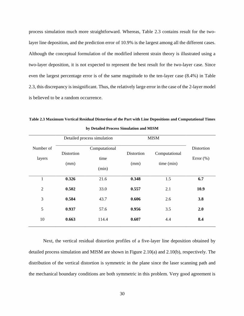
30

process simulation much more straightforward. Whereas, Table 2.3 contains result for the two-

layer line deposition, and the prediction error of 10.9% is the largest among all the different cases.

Although the conceptual formulation of the modified inherent strain theory is illustrated using a

two-layer deposition, it is not expected to represent the best result for the two-layer case. Since

even the largest percentage error is of the same magnitude to the ten-layer case (8.4%) in Table

2.3, this discrepancy is insignificant. Thus, the relatively large error in the case of the 2-layer model

is believed to be a random occurrence.

Table 2.3 Maximum Vertical Residual Distortion of the Part with Line Depositions and Computational Times

by Detailed Process Simulation and MISM

Number of

layers

Detailed process simulation MISM

Distortion

Error (%) Distortion

(mm)

Computational

time

(min)

Distortion

(mm)

Computational

time (min)

1

2

3

5

10

0.326

0.502

0.584

0.937

0.663

21.6

33.0

43.7

57.6

114.4

0.348

0.557

0.606

0.956

0.607

1.5

2.1

2.6

3.5

4.4

6.7

10.9

3.8

2.0

8.4

Next, the vertical residual distortion profiles of a five-layer line deposition obtained by

detailed process simulation and MISM are shown in Figure 2.10(a) and 2.10(b), respectively. The

distribution of the vertical distortion is symmetric in the plane since the laser scanning path and

the mechanical boundary conditions are both symmetric in this problem. Very good agreement is

31

observed by comparing the two figures. Both the accuracy and efficiency of the proposed method

are further validated.

(a) (b)

Figure 2.10 Vertical Residual Distortion (Unit: m) of the 5-Layer Line Deposition by (a) the Detailed Process

Simulation and (b) the MISM

In terms of computational efficiency, the computational times of the detailed process

simulation and the MISM are also shown in Table 2.3. Generally, a ~20x speedup can be achieved

using the MISM as compared with detailed process simulation. Especially for the depositions

containing more layers, the computational efficiency becomes higher (see 10-layer case in Table

2.3). Clearly, with more development, the proposed method has great potential in fast prediction

of residual deformation in an AM part.

2.3.2 Rectangular Contour Wall Deposition Model

In order to further demonstrate accuracy of the proposed method, the rectangular contour

wall deposition shown in Figure 2.11 is investigated here. In the printing process, the laser

scanning path is counterclockwise as illustrated by arrows in the figure. Each side of the model

can be considered as an independent single-walled deposition, since the intersection of any two

32

neighboring sides is relatively small. Since an intermediate state containing a stable mechanical

boundary is critical in the proposed theory, the intermediate state of the elements in the layer of

interest is defined as the moment when the overlaid layer on the same side has just been deposited.

Figure 2.11 Laser Scanning Path of the Rectangular Contour Deposition

First, detailed process simulation is conducted for the rectangular contour wall with

different number of layers. In particular, for the five-layer rectangular contour wall, dimension of

the substrate is set to 101.6×101.6×3.18 mm3 in order to be consistent with the experimental setup.

For other cases, the size of the substrate is the same as in the first example. Geometrical parameters

such as the length (L), width (W), thickness (T) and height (H) of the rectangular contour

depositions are shown in Figure 2.12 and also listed in Table 2.4 below. The process parameters

employed are as follows: Laser power 300W, scan velocity 2.0 mm/s, and powder feed rate of 6

RPM. In addition, to ensure numerical convergence of the detailed process simulation for the five-

layer contour, the substrate is meshed using two layers of elements in the thickness direction, while

three layers of elements are employed for the other cases. To ensure the choice does not create an

unfair comparison, the influence of the element mesh to the numerical simulations has been

33

investigated through a series of process simulations. For the five-layer contour deposition case,

two cases were investigated where the substrate was meshed into one and two elements in the

dimension of thickness, respectively. It is found that the influence by the element mesh of the

substrate to the entire residual distortions is negligible, which indicates that the substrate mesh is

not a concern to the validation of the proposed method.

Figure 2.12 Illustration of the Geometry of the Rectangular Contour Deposition

Table 2.4 Geometrical Parameters of the LENS Rectangular Contour Depositions

Number of layers Length /mm Width /mm Thickness /mm Height /mm

1 41.86 22.37 2.52 0.90

2 41.86 22.37 2.20 1.90

4 31.80 19.80 2.10 4.10

5 41.86 22.37 2.72 4.43

Through detailed process simulation and MISM, the maximum residual distortion in the

vertical direction for the rectangular contours with different number of layers is listed in Table 2.5.

34

The difference between the results obtained by the two different methods is very small, which

indicates good accuracy for the proposed method. Although the substrate deformation results are

much more consistent for layers 2 through 5 cases, no obvious trend is found in the substrate

deformation results for the different number of deposition layers. Regarding a larger error in the

one-layer case, a reasonable explanation is that it may not be so robust to identify the intermediate

state of a long single layer deposition using exactly the same way established based on the multi-

layer LENS process. Since the difference was acceptable when the same way of identifying the

intermediate state was applied in all the cases, the one-layer contour case was still included to

demonstrate the efficiency of the proposed method. In addition, the computational times of the

detailed process simulation and the MISM are shown in Table 2.5. The computational efficiency

has a significant improvement (e.g. nearly 80x speedup for the 5-layer case) due to benefit of the

proposed method.

Table 2.5 Maximum Vertical Residual Distortion of the Part with Rectangular Contour Deposition and

Computational Times by the Detailed Process Simulation and the MISM

Number

of layers

Detailed process simulation MISM

Distortion

Error (%)

Distortion

(mm)

Computational time

(min)

Distortion

(mm)

Computational time

(min)

1

2

4

5

0.499

0.776

0.950

1.157

134.0

153.6

398.1

439.2

0.432

0.798

0.973

1.131

2.4

3.2

4.2

4.8

13.4

2.8

2.4

2.2

35

Meanwhile, the respective vertical displacement profiles of the rectangular contour wall

with two layers and five layers obtained from the two different methods are shown in Figures. 2.13

and 2.14.

(a) (b)

Figure 2.13 Vertical Residual Distortion (Unit: m) of the Part with the 2-Layer Contour Deposition (a) by the

Detail Process Simulation and (b) by the MISM

(a) (b)

Figure 2.14 Vertical Residual Distortion (Unit: m) of the Part with the 5-Layer Contour Deposition (a) by

Detailed Process Simulation and (b) by the MISM

As can be seen, the maximum residual distortion occurs at the free end of the substrate in

the vertical direction. Clearly, the distribution of the vertical displacement field obtained in two

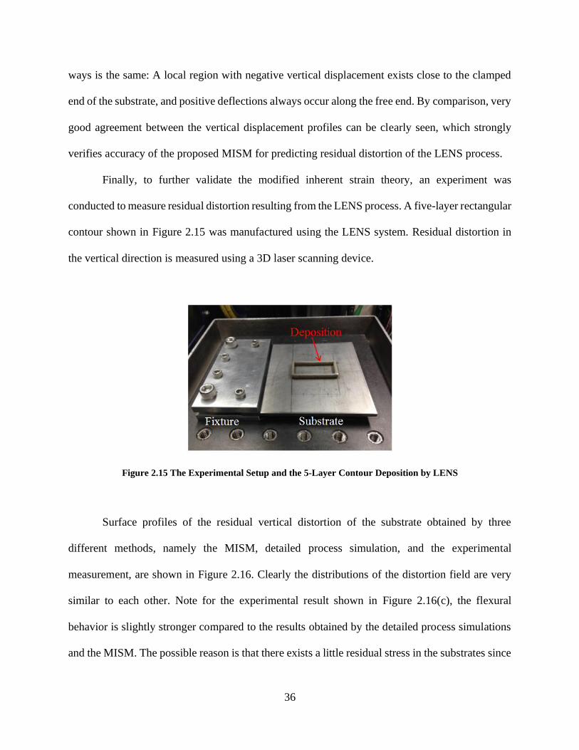
36

ways is the same: A local region with negative vertical displacement exists close to the clamped

end of the substrate, and positive deflections always occur along the free end. By comparison, very

good agreement between the vertical displacement profiles can be clearly seen, which strongly

verifies accuracy of the proposed MISM for predicting residual distortion of the LENS process.

Finally, to further validate the modified inherent strain theory, an experiment was

conducted to measure residual distortion resulting from the LENS process. A five-layer rectangular

contour shown in Figure 2.15 was manufactured using the LENS system. Residual distortion in

the vertical direction is measured using a 3D laser scanning device.

Figure 2.15 The Experimental Setup and the 5-Layer Contour Deposition by LENS

Surface profiles of the residual vertical distortion of the substrate obtained by three

different methods, namely the MISM, detailed process simulation, and the experimental

measurement, are shown in Figure 2.16. Clearly the distributions of the distortion field are very

similar to each other. Note for the experimental result shown in Figure 2.16(c), the flexural

behavior is slightly stronger compared to the results obtained by the detailed process simulations

and the MISM. The possible reason is that there exists a little residual stress in the substrates since

37

some machining treatment was done in the manufacturing process. The LENS process may

contribute to releasing the residual stress in the substrate, generate some bending and affect the

distribution of the distortions. This explanation is acceptable since similar observations had been

obtained in other experiments using the same substrates.

Figure 2.16 Vertical Residual Distortion (Unit: mm) of the Substrate with LENS Deposition of 5-Layer

Rectangular Contour by (a) MISM (b) Detailed Process Simulation (c) Experimental Measurement

In addition, both the minimum and maximum vertical residual distortions of the substrate

are listed in Table 2.6. A concern is that the minimum distortion magnitudes are roughly 50 percent

different from the experiment and two possible reasons are provided. First, the resolution of the

laser scanning device is ±0.075mm, which may induce some error to the deformation

measurement. As seen in the table, the magnitudes of the minimum distortion obtained by the

detailed process simulation and the MISM are very small and close to the measurement precision.

The experimental measurement of the residual distortion may have some uncertainty caused by

system errors, leading to slightly larger magnitudes (see Table 2.6). Second, the large error also

has to do with the inaccurate boundary condition of the clamp since the minimum distortion

location is close to the clamp. In the experiment, the fixtures were clamped by only several bolts

as seen in Figure 2.15. However, all the nodes of the fixtures were fixed strictly as the mechanical

38

boundary conditions in the simulations. As a result, a relatively smaller distortion is seen in the

simulation results, but generally, the maximum residual distortions are in excellent agreement with

each other. From these results, the effectiveness and accuracy of the MISM are both proved.

Table 2.6 Vertical Residual Distortion (Unit: mm) of the Substrate with a LENS Deposited 5-Layer

Rectangular Contour in Three Different Ways

Minimum Maximum

Relative error of the

maximum distortion (%)

MISM

Detailed process simulation

Experimental measurement

-0.121

-0.107

-0.217

1.131

1.157

1.281

11.7

9.7

---

In this section, all the deposition lines were simulated and the inherent strains for the entire

part were extracted and applied back to the LENS build. Compared to the thermomechanical

simulation results, many features of the residual deformation can still be seen when this full-scale

inherent strain approach is employed. This full-scale inherent strain approach is simply used to

verify the accuracy of the modified model proposed in Eq. (2.16).

2.4 Mean Inherent Strain Vector Approach

For single-walled structures containing many layers, in order to achieve satisfactory results,

typical inherent strains extracted from two successive line deposition layers can ensure prediction

accuracy. It is unreasonable to only simulate a one-layer line deposition model for extracting

typical inherent strains because the re-melting process is not considered in this one-layer process

39

model. On the other hand, in the LENS processing of the single-walled model, the deposited

materials have enough time to cool down since the laser scanning speed is low (2 mm/s) and the

length of the deposition line is large. Moreover, the large substrate is also made of the same Ti64

material with the deposition. Thus, it is not necessary to simulate more than two deposition lines

to extract the inherent strains, since it can be assumed that most of the deposition lines experience

the same melting and re-melting process.

To verify the above statement is correct, a representative volume of the full-scale two-layer

and three-layer line deposition model is employed in the detailed process simulation to extract the

inherent strains, respectively. As depicted in Figure 2.8, the inherent strains are averaged over

entire length of the deposition line. Hence a mean strain vector of (-0.0070, -0.002, 0.008) is

obtained for the two-layer model, while (-0.0073, -0.003, 0.007) is obtained for the three-layer

case. The inherent strain vector is converted to orthogonal CTEs and uniformly assigned to the

multi-layer models as thermal material properties. In the solution, the elements of the multi-layer

models are activated layer-by-layer and unit temperature is applied as the external load. The results

for the three-layer and five-layer wall structures obtained by the layered ISM and detailed process

simulation are shown in Table 2.7. The errors are a little larger than the results obtained from full-

scale detailed simulation of the entire build shown in Table 2.3. A possible reason is that the mean

inherent strains, which are accurate only in the middle region of a large part, are applied uniformly

to all the elements including those close to the surface. Despite the difference, very good

agreement is shown between the results obtained from the two different methods. the results

demonstrate that only two deposition layers are needed in the representative volume model to

ensure accuracy. However, if still higher accuracy is desired, three or more deposition layers may

be employed to extract the inherent strains.

40

Table 2.7 Maximum Vertical Residual Distortion of the Substrate with LENS Deposited 3- and 5-Layer

Straight Wall Structure and Computational Times by Detailed Process Simulation and Layered ISM

Number of

layers

Detailed process simulation

Simulation based on mean inherent strain

Extracted from 2-layer

model

Extracted from 3-layer

model

Distortion

(mm)

Computational

time (min)

Distortion

(mm)

Computational

time (min)

Distortion

(mm)

Computational

time (min)

3

5

0.584

0.937

43.7

57.6

0.534

1.024

2.1

2.5

0.553

1.063

2.8

3.2

To verify that the proposed method is an efficient approach with low computational effort,

comparison between the proposed method and detailed process simulation has been provided in

terms of the computational effort required. Table 2.8 shows computational times for the straight

five-layer single-walled deposition case in the full-scale detailed process simulation and the

MISM, respectively. Note that the proposed method allows the computational time to be reduced

by ~20 times. Clearly, this comparison demonstrates the good computational efficiency of the

proposed method.

41

2.5 Practical ISM based on Small-Scale Detailed Simulation

2.5.1 Description of Proposed Method

Inspired by the assumption that nearly all the elements in a deposition line experience

similar physical process, the entire length of a long deposition line does not need to be considered

in the representative volume model. Therefore, for the LENS process concerned in this

dissertation, how to determine a reasonable small-scale model has been investigated to extract the

mean inherent strains for different single-walled structures. This section introduces details of the

small-scale model with particular emphasis on the following three aspects:

(1) Determination of the small-scale model

The geometry of the small-scale model for the LENS process should be a two-layer line

deposition model. It is also reasonable to use a three-layer deposition model if the computational

cost can be afforded. However, the benefit of utilizing a three-layer deposition as the small-scale

model is little, as the mean inherent strains extracted from the two-layer and three-layer single-

walled model are very close to each other.

The size of the two-layer small-scale model depends on the specific DED process

parameters including laser power, scanning speed and powder feed rate. For the process parameters

employed for LENS processing of Ti64 in this dissertation (laser power 300W, scanning speed 2.0

mm/s and powder feed rate 6~8 rpm), the size of the small-scale two-layer model can be defined

as 20×2.0×1.8 mm3 as shown in Figure 2.17(a). Note the length for the small-scale process model

should be selected to ensure that the temperature along the scan line in the simulation reaches

steady state. (The inherent strains will then be extracted from the steady state region as steady

state behavior is dominant in most structures of interest.) The heat source should move far away

42

from the starting end to ensure that the temperature contour maintains a stable shape with a comet-

like tail over the layer (see Figure 2.17(b), for example). The mesh dimension of the two-layer

small-scale model is shown in Figure 2.17(a). As a common practice [27, 28, 35], one element

through the thickness is employed to model one single layer. For the element mesh along the laser

scanning direction, given the laser beam diameter (~0.6 mm) of the LENS machine, the layer is

meshed with 40×3 elements in the length and width dimension (see Figure 2.17(a)). Employing

the element birth and death method, 50 load steps are used to simulate the deposition process of

one single layer.

(a) (b)

Figure 2.17 Typical Features of the Small-Scale Model: (a) Geometry and Mesh Model and (b) Stabilized

Temperature Contour in a Deposition Layer

(2) Evaluation of mean inherent strain

After the small-scale simulation is finished, the elastic and plastic strain history of any

material point in the deposition can be recorded conveniently using APDL commands. Material

points in the centerline of bottom layer in the small-scale model are selected as the sampling points

to compute the mean inherent strain. The elastic and plastic strains in the intermediate and steady

43

states of the selected sampling points are obtained from the small-scale simulation results. Then

the inherent strains at each sampling point can be computed based on the modified inherent strain

definition given in Eq. (2.16). For the strain component parallel to the laser scanning direction, the

inherent strains are summed up and averaged over the entire layer dimension to obtain the mean

inherent strain component. Similarly, the same procedure is carried out for the remaining two

inherent strain components perpendicular to the laser scanning path and in the build direction. In

this manner, the three normal components of the mean inherent strain vector can be evaluated. In

this section, the mean inherent strain vector based on the small-scale model is determined to be (-

0.0069, -0.002, 0.008) and will be applied to the rectangular contour deposition model to verify its

accuracy.

(3) Application to a different single-walled structure

These normal inherent strains are averaged into an inherent strain vector as discussed

above. To implement this conveniently in commercial FEA software, the mean inherent strain

vector is treated as orthotropic CTEs for the large model. The rectangular contour wall deposition

model is considered as a different part to illustrate the application of the mean inherent strain

extracted from the small-scale detailed simulation model. Note that the in-layer components of the

mean inherent strain vector correspond to the directions parallel and perpendicular to the laser

scanning direction. However, since the laser scanning changes direction on different sides of the

rectangular contour deposition model and forms a closed contour path, a reasonable way is to apply

the averaged magnitude for the in-layer components of the mean inherent strain vector to the layers

containing different laser scanning paths. Therefore, the mean inherent strain vector for each layer

of the rectangular contour becomes (-0.0045, -0.0045, 0.008) after averaging and is then applied

uniformly to each layer of the rectangular contour wall model. The layers in the large model are

44

activated layer-by-layer, and a unit temperature increase is applied to the newly activated layer to

introduce the inherent strains as initial strains. Generally, the mean inherent strain obtained through

the small-scale simulation can be applied to different single-walled structures and predict residual

deformation efficiently.

2.5.2 Results and Discussion

The predicted maximum vertical deformation of the 5-layer and 10-layer rectangular

deposition model using the new mean inherent strain vector is shown in Table 2.8 together with

results obtained from full-scale detailed process simulation.

Table 2.8 Maximum Vertical Deformation of the Rectangular Contour Deposition Model Using Full-Scale

Process Simulation and the MISM based on Small-Scale Process Simulation

Cases

Maximum vertical deformation (mm)

Full-scale process

simulation

MISM Error (%)

5-layer 1.157 1.181 2.1

10-layer 1.622 1.780 9.7

In addition, the vertical residual deformation profile of the ten-layer rectangular contour

deposition model is shown in Figure 2.18. Clearly, compared with those full-scale simulation

results, good agreement can be observed, and the MISM based on the small-scale simulation is

successfully validated when applied to a different model. Nonetheless, a possible explanation for

the relatively large error in the ten-layer case is that, during deposition of large parts, the workpiece

45

experiences different thermal energy transfer. As a result, the re-melting zone changes during the

deposition process, and it is normally larger with increasing distance from the substrate. This

phenomenon could affect the extracted inherent strains, and it may be inappropriate to use the

same mean inherent strain vector for all the layers in a large AM build.

(a) (b)

Figure 2.18 Predicted Distribution of Vertical Residual Deformation (Unit: m) of the 10-Layer Rectangular

Contour Deposition by (a) Full-Scale Process Simulation (b) Mean Inherent Strain Vector Method

Regarding efficiency of the proposed method, the computational times of the two new

cases of the five-layer and ten-layer rectangular contour deposition models are shown in Table 2.9.

The time needed for the small-scale simulation model (33.8 mins) has been added to the total

computational time for the modified inherent stain method since it also takes time to evaluate the

mean inherent strain vector. As shown in the table, even with the small-scale simulation time

included, the MISM is still much more efficient (10~15x speedup) than the full-scale detailed

thermomechanical simulation. And if only the time it takes to execute the MISM is considered,

the improvement of the computational efficiency can be nearly 80 times.

46

Table 2.9 Comparison of Detailed Process Simulation and the MISM in Terms of Computational Efforts

Required for the 5-Layer and 10-Layer Rectangular Contour Deposition Model

Cases

Computational time (min)

Full-scale detailed

process simulation

MISM

Including small-scale

simulation

Excluding small-

scale simulation

5-layer 439.2 38.4 4.6

10-layer 610.2 42.2 8.4

Additionally, the same mesh is used when the obtained inherent strains are applied back to

the deposition models in this chapter. The benefit of doing this is that the inherent strains can be

applied in a convenient element-by-element manner. If the mesh size of the detailed simulation

model is different from that used for the estimation of the residual distortions, the calculated

inherent strains could be mapped to the model as a function of the location of the elements. For

the model used for the detailed process simulation, the locations of those elements in the HAZ can

be normalized to a standard range as seen in Figure 2.8. Then for the model with a different mesh

used for the prediction of the residual distortions, as for any element in the HAZ, according to its

normalized location, the amount of the inherent strains to be assigned to the element can be

calculated by interpolation using the normalized curves.

2.6 Conclusions

In this chapter, the MISM is proposed for fast prediction of residual distortion of single-

walled structures produced by a representative DED process in LENS. Specifically, a modified

47

model is proposed to estimate the inherent strains from detailed process simulation, which are then

applied to the part model to perform a layer-by-layer static analysis to simulate residual distortion.

To validate the proposed model, the inherent strains obtained from full-scale detailed simulation

of the entire structure under consideration are applied back to the structure to predict residual

distortion by static equilibrium analysis. The structures employed to validate the model include a

single wall and rectangular contour wall by the LENS process. The accuracy and efficiency of the

proposed method has been demonstrated by both numerical examples and experiments.

As a first step to make the proposed method practical, the mean inherent strain concept is

then proposed and extracted based on full-scale two-layer and three-layer line deposition models.

Numerical examples have demonstrated that the mean inherent strain can be applied to single-

walled structures having more layers to accurately predict the residual deformation much faster.

To make the method truly practical, a small-scale detailed simulation model is proposed to extract

the mean inherent strains, which are then applied to different single-walled structures for fast

residual deformation prediction. Simulation results show that the MISM is quite efficient, while

the residual distortion of AM parts can be accurately computed within a short time.

The assumption that most of the deposition lines experiences the same melting and re-

melting process in the AM process may not be true in some cases. When the scan speed is high

and the part is large, the workpiece may experience different thermal energy transfer due to the

boundary effects of the substrate and the previous deposition layers with high temperature. In other

words, the sampling positions of the small-scale model from the large part may also have some

effects on the extracted inherent strains. To tackle this problem, further research is needed to

investigate the temperature gradient in the deposition by performing many more detailed process

simulations and experiments.

48

The modified inherent strain model is proposed based on single line depositions on top of

each other, and hence validity of the model has been demonstrated only on single-walled structures

in this dissertation. The proposed model will need to be extended in order to treat more complex

geometries consisting of scan lines not only on top of each other but also next to each other. For

a large AM build, clearly it is impossible to simulate all the lines and layers before extracting the

overall inherent strains. In addition, usually complex geometries may be deposited using complex

laser scanning patterns in the AM process including DED and PBF. The influence on the inherent

strains by the process parameters such as the laser scanning path needs to be considered further.

Thus, the detailed depositing path needs be modeled in the simulation of a local region of the large

part. This also means that simulating only a straight deposition line is not sufficient for computing

the inherent strains accurately for complex geometries. Rather, a small section may be used as the

representative volume to obtain the inherent strains necessary to simulate deformation of a large

complex part efficiently. Further research is needed to investigate this approach and the associated

accuracy and efficiency.

49

3.0 MISM for PBF Components

3.1 Current Simulation Methods for PBF Components

The powder bed fusion (PBF) process is currently the most popular AM process for

manufacturing complex metal parts in the industry. For example, techniques such as direct metal

laser sintering (DMLS) [32, 60, 61], selective laser melting (SLM) [62-64] and electron beam

melting (EBM) [65-68] are all powder bed based. In general, a metal component is built out of a

powder bed via repeated micro-welding process. At the macroscopic scale, different AM systems

involving a high energy beam are generally based on similar physical process like melting and

solidification of metal materials. Typically, large temperature gradient and high cooling rate will

occur due to intensive heat source and large local energy density [55], which consequently leads

to large thermal strain and hence significant residual stress or deformation in the metal

components. These are both undesirable as large residual deformation makes it difficult to post-

process parts to achieve the desired dimensional accuracy, and residual stress can cause cracking

during the build. Therefore, it is of critical importance to predict residual stress and deformation

in the process such that the quality of the printed components can be guaranteed.

In the past, residual deformation and stress were predicted through fully coupled

thermomechanical simulations [28, 69, 70] based on heat source models [49, 53, 71], which is very

time-consuming. Moreover, for the complex metal parts, it is very difficult to compute the residual

deformation through these detailed process simulations, since a part may contain thousands of thin

layers containing numerous scan tracks. Limited by computational power, it is very difficult to

predict residual deformation of large-scale AM parts by detailed thermomechanical simulation

50

directly. Even with a coarse layer-by-layer analysis pattern [72, 73], it still takes many hours to

obtain the final residual deformation of the AM builds. To achieve a faster prediction, some

alternatives were developed based on welding mechanics such as the inherent strain theory [37,

39, 40]. This method was first established to calculate the residual deformation in metal welding

problems. However, conventional ISM was proved to be inaccurate when applied to predict

residual deformation in complex AM process. Similarly, the applied plastic strain method [42, 43]

was proposed to simulate residual deformation of an LENS deposited part. However, it was found

that the accuracy of this method is not adequate when applied to large AM builds. In the past years,

Keller et al [45] and Alvarez et al [74] proposed some possible values of inherent strain used to

efficiently predict the residual deformation of the AM components. Nonetheless, the detailed

theory and method of determining inherent strain in the AM builds were not presented. Recently,

an empirical methodology was proposed to determine the inherent strain values in the SLM-printed

components [75]. Through iteratively optimizing the difference between the predicted residual

distortions and the experimental results of double cantilever beams, reasonable inherent strain

values can be determined to ensure good prediction accuracy compared with the experiments. This

empirical method is expensive since many metal samples need to be manufactured and large

computational work is required in the numerical optimization process. In addition, the present

authors proposed the modified inherent strain theory [76] to compute accurate inherent strain in

single-walled structures consisting of single line depositions by the LENS process. However, the

validity of the modified theory has not been demonstrated when applied to the DMLS process

employing more complex scanning strategies such as the rotational laser scanning paths in

different deposition layers. Moreover, it has not been fully revealed how to predict the residual

51

distortion accurately and efficiently for a large and geometrically complex DMLS component

containing many thin layers based on the modified inherent strain model.

3.2 MISM Adapted for PBF Process

In a typical AM process, new layers are formed out of the metal powder bed all the time

during the multi-track laser fusion process, which will cover those lower layers and act as a

mechanical constraint for them. The layer-by-layer shrinkage of the upper layers will also

contribute downward to the evolution of the elastic deformation and stress in the lower depositions.

Consequently, the assumption in the early method that only the plastic strain in the final

equilibrium state of the weld matters as the inherent strain will be invalid when applied to the

layered AM process. The inelastic strains are highly dependent on the boundary conditions

including mechanical and thermal boundary, plate dimensions, and fixtures like the large substrate

as the constraint in the DMLS process, etc. The inherent strains in the metal part have to be

determined case by case since many factors, even like the input laser power can influence the time-

dependent accumulation of inelastic strains. This makes the application of this method expensive

in time. Nonetheless, physically in the AM builds, many layers are subjected to same kind of

thermal expansion and shrinkage caused by the moving thermal loading, and similar mechanical

restraints like the constraint by the already deposited cooled layers. As a result, the accumulation

of their inelastic/inherent strains will be very similar. Therefore, it is believed that only a small

representative volume needs to be fully simulated to look into the accumulation of the inelastic

strains in the thermal and mechanical equilibrium process of AM. Then the typical inherent strains

52

can be extracted and applied to the layers in the large part. In this way, significant gain in time can

be obtained.

In order to obtain accurate inherent strain values, the amount of thermal strain that is

converted into mechanical strain responsible for residual deformation (so-called inherent strain)

needs to be captured. In the proposed theory, the inherent strain in the layer-by-layer AM process

is a processing-history-dependent quantity, rather than being only dependent on the final cooled

state as in the original theory. Besides the generated plastic deformation as a definite source in the

proposed inherent strain model, new strain terms are added to account for the evolving elastic

deformation due to the layer-by-layer shrinkage in the cooling process, which represents

conversion of some of the thermal strain coupled with the influence of the inter-layer constraint.

Therefore, the modified inherent strain theory is proposed specifically to adapt to the AM process,

and two major sources for the inherent strain are considered.

(1) Contribution from plastic deformation. Large compressive plastic strain is generated

once the powder is sintered by the laser beam and rapid solidification of material occurs. The

plastic strain incurred during rapid solidification is considered to be a direct conversion of the

thermal strain. Given a material point already deposited, in the following cooling-reheating-

cooling process, the plastic strain changes due to the temperature increase and decrease. However,

compared with the evolution history of the elastic strain, the change of the plastic strain is not so

significant. For convenience of discussion, the instant when the compressive plastic strain reaches

its maximum due to the rapid solidification phenomenon is defined as the “intermediate state”.

Based on the above assumption, contribution of the plastic deformation to the inherent strain of

the AM process is written as:

𝜺𝑝∗ = 𝜺𝑝

𝐼 (3.1)

53

(2) Contribution from thermal shrinking coupled with inter-layer effect. In the original

method, the induced inherent strain in the welded part is assumed to be equal to the residual plastic

strain, given that the thermal strain quickly vanishes after the heating-cooling cycle and thus has

no effect on the change of mechanical strain. In order to adapt the original ISM to model the metal

AM process, the influence of thermal shrinkage is further considered coupled with the evolving

mechanical constraint and inter-layer effect due to the deposition of new layers on the residual

deformation and stress. For a material point under consideration, its intermediate state is

considered the beginning of the accumulation of the elastic deformation. After the intermediate

state, the elastic deformation at any material point will be changed by thermal shrinkage of the

surrounding solid and the layer-by-layer overlaid solid materials until the entire part reaches the

end of the cooling process, which is defined as the “steady state”. This change of elastic strain

during the cooling process represents the conversion of thermal strain into mechanical strain that

needs to be accounted for in the modified model for AM. Since no heat transfer simulation is

performed in the original ISM, this change in elastic strain is thus added to the plastic strain, which

becomes the modified model for AM. In fact, the property of the additional source in the modified

inherent strain model is still not elastic. The contribution to the inherent strains in the AM process

can be written as:

𝜺𝑡ℎ∗ = 𝜺𝑒

𝐼 − 𝜺𝑒𝑆 (3.2)

where 𝜺𝑒𝐼 and 𝜺𝑒

𝑆 denote the elastic strain at the intermediate and steady state of the specific AM

process, respectively. The intermediate state is the same with the one defined in Eq. (2.15).

Finally, the modified inherent strain model proposed can be written as:

𝜺∗ = 𝜺𝑝∗ + 𝜺𝑡ℎ

∗ (3.3)

As the modified theory indicates, the residual deformation is inherently induced by the heat

input and influenced by the inter-layer effects of the evolving mechanical boundaries as new layers

54

are deposited onto the previous ones. The inherent strain is employed to quantitatively capture the

deformation considering the thermal history and the inter-layer mechanical constraint in the AM

process. In practice, the inherent strain model will be utilized to extract the typical inherent strain

values from a small-scale detailed process simulation for a given AM process. And then the

obtained strain values will be applied to the entire metal part to predict the residual distortion. This

method is proved to be valid when the process has a build pattern that repeats itself periodically,

as will be demonstrated for the DMLS process next.

3.3 Calculation and Application of Inherent Strain

3.3.1 Calculation of Inherent Strain

The small-scale detailed process simulation of the DMLS processing of Ti64 and Inconel

718 is presented below based on FEA. Since the detailed process model for DMLS in this chapter

is adapted from that of the LENS process discussed in Ref. [55], only the pertinent details specific

to the DMLS process are given and only a brief description of other details is provided hereby. In

the detailed simulation, temperature-dependent material properties such as the coefficient of

thermal expansion (CTE), Young’s modulus, and yield strength [30, 55] are employed. The DMLS

system has different scanning modes using different process parameters. The core-skin mode will

be simulated as it is the dominant mode for printing the core volume of a metal component. The

process parameters of this print mode for Ti64 and Inconel 718 are listed in Table 3.1.

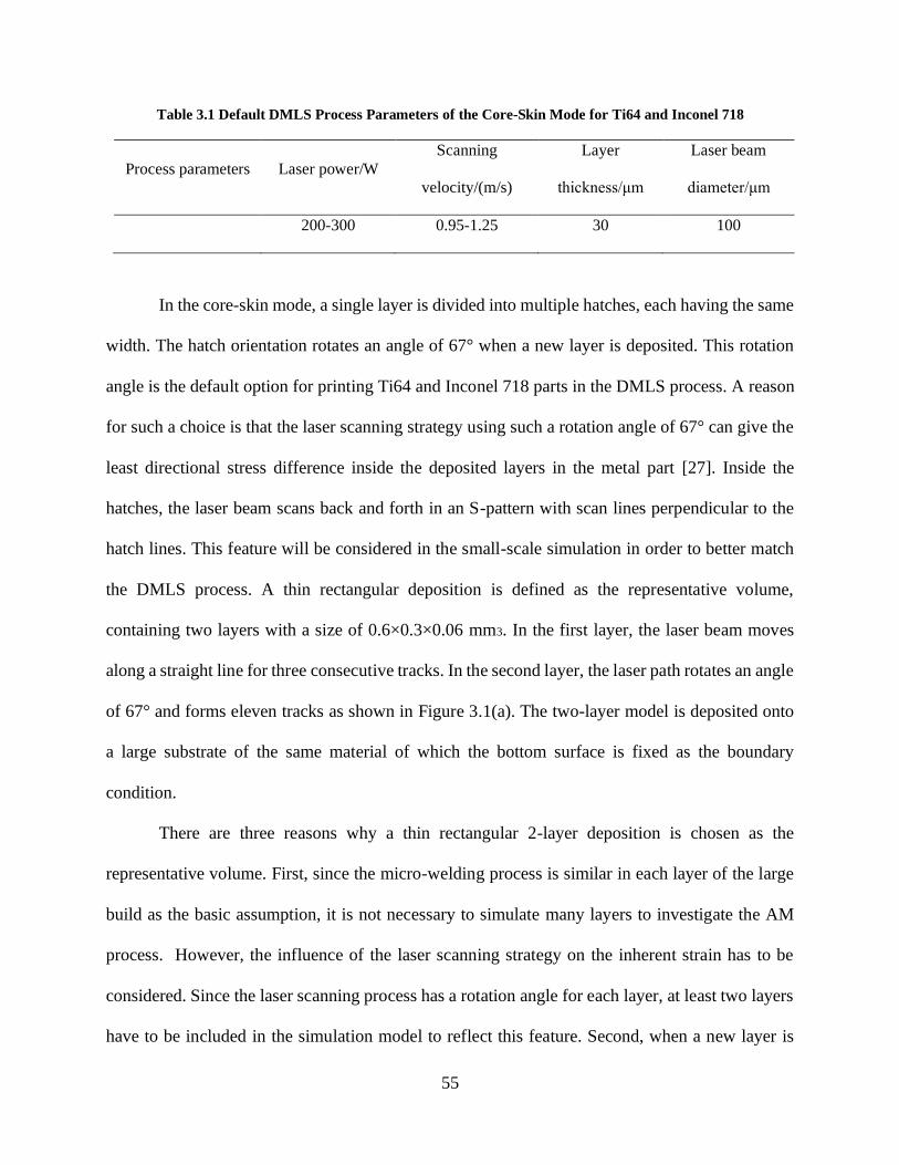
55

Table 3.1 Default DMLS Process Parameters of the Core-Skin Mode for Ti64 and Inconel 718

Process parameters Laser power/W

Scanning

velocity/(m/s)

Layer

thickness/μm

Laser beam

diameter/μm

200-300 0.95-1.25 30 100

In the core-skin mode, a single layer is divided into multiple hatches, each having the same

width. The hatch orientation rotates an angle of 67° when a new layer is deposited. This rotation

angle is the default option for printing Ti64 and Inconel 718 parts in the DMLS process. A reason

for such a choice is that the laser scanning strategy using such a rotation angle of 67° can give the

least directional stress difference inside the deposited layers in the metal part [27]. Inside the

hatches, the laser beam scans back and forth in an S-pattern with scan lines perpendicular to the

hatch lines. This feature will be considered in the small-scale simulation in order to better match

the DMLS process. A thin rectangular deposition is defined as the representative volume,

containing two layers with a size of 0.6×0.3×0.06 mm3. In the first layer, the laser beam moves

along a straight line for three consecutive tracks. In the second layer, the laser path rotates an angle

of 67° and forms eleven tracks as shown in Figure 3.1(a). The two-layer model is deposited onto

a large substrate of the same material of which the bottom surface is fixed as the boundary

condition.

There are three reasons why a thin rectangular 2-layer deposition is chosen as the

representative volume. First, since the micro-welding process is similar in each layer of the large

build as the basic assumption, it is not necessary to simulate many layers to investigate the AM

process. However, the influence of the laser scanning strategy on the inherent strain has to be

considered. Since the laser scanning process has a rotation angle for each layer, at least two layers

have to be included in the simulation model to reflect this feature. Second, when a new layer is

56

deposited, the re-melting process of the previous deposition has important influence on the

redistribution of the elastic and plastic strain in the deposited layers. Meanwhile, the inter-layer

effect between two adjacent layers will also affect the mechanical strain in the deposition. A 2-

layer deposition model is able to consider all these important factors mentioned above. Third, the

detailed thermomechanical simulation is computationally expensive because very fine mesh and

small time steps have to be employed to ensure the accuracy of the numerical analysis. In order to

reduce the computational cost, simulating many layers in the representative volume should be

avoided. Thus, the thin rectangular 2-layer model as the representative volume is chosen for the

small-scale simulation. More thin layers can be created below the concerned layers to represent

the already deposited ones. Since the temperature drops very quickly in the already deposited

layers, it is acceptable to use room temperature as the initial thermal boundary condition for those

layers. The large substrate then provides the appropriate thermal and mechanical boundary

conditions for the entire model. However, in this way the small-scale model will give similar

inherent strain results compared with the only 2-layer model according to the simulation trials.

This phenomenon is reasonable because the already deposited layers work like the substrate

constraint. As a result, the influence is negligible when only large substrate without already

deposited layers is used as the constraint for the representative volume model. Compared with the

manner of extracting the inherent strain values for LENS based on a 2-layer small-scale simulation

in Ref. [76], a lot more deposition lines are modeled around a concerned line in the lower layer

out of the 2-layer model. The reason is that the DMLS process has higher and more localized laser

intensity and usually its physical deposition layers are much thinner than those in LENS. The

neighboring deposition lines including the adjacent upper layer will affect the mechanical strain

57

evolution of any concerned material point in one deposition line of the lower layer. As a result, the

inherent strain for the lower layer will also be influenced greatly.

(a) (b)

Figure 3.1 Small-Scale Model: (a) a 2-Layer Representative Volume on the Bottom-Fixed Substrate and the

Laser Scanning Strategy, and (b) Illustration of the Intermediate and Steady State of a Ti64 Material Point

(Black Dot)

The actual process parameters for Ti64 in the micro-mechanical model are as follows: laser

power of 280 W, laser beam diameter of around 100 μm, scanning speed of 0.95 m/s and layer

thickness of 30 μm. As for Inconel 718, the laser power is 285 W and scanning speed is 1.0 m/s.

The other parameters are the same with Ti64, for example, the laser energy absorption efficiency

of 50% is used for both materials. The double-ellipsoidal heat source model [53] is employed in

the small-scale process simulation. Detailed mathematical description of this heat source model

can be found in Refs. [53, 55]. Its major feature is that the respective lengths of the longitudinal

(𝑎), transverse (𝑏) and through-the-depth (𝑐) semi-axes of the ellipsoidal laser beam can be

different. Values of the semi-axes of the heat source model are determined based on the practical

process parameters in Table 3.1. For both materials, the values of 𝑎 and 𝑏 are equal to the radius

58

(50 μm) of the laser beam. The value of the depth 𝑐 is determined as 90 μm through experiments,

which equals the thickness of three thin layers in the DMLS process.

The involved laser scanning pattern in this chapter is a typical scanning strategy in the

DMLS process. In addition, besides the core-skin scanning mode, there are other scanning modes

such as the island scanning used by other AM systems. However, even though the scanning

patterns are different for different layers, the proposed method can still be employed. When more

complicated scanning patterns are concerned, a small representative volume which contains only

a few layers corresponding to the typical scanning patterns for different layers needs to be found.

As long as the representative volume is established and the small-scale process simulation can be

implemented, the MISM can be employed, for both the extraction of the inherent strain values and

the prediction of the residual deformation. Nonetheless, the sacrifice is that the computational cost

will be expensive since more layers have to be considered to reflect the different laser scanning

patterns for different layers.

Based on the small-scale simulation of the two-layer Ti64 model, one typical material point

(black dot in Figure 3.1(b)) is chosen and the longitudinal elastic and plastic strain in the direction

of the horizontal laser scanning path (see first layer in Figure 3.1(a)) are plotted in Figure 3.1(b).

The drastic jumps of the curves indicate the heating and re-heating when the laser beam passes the

point (left temperature map in Figure 3.1(b)). And the nearly flat sections indicate the steady

cooling process (right temperature map in Figure 3.1(b)). The intermediate and steady states of

any material point in the DMLS process will be identified based on the strain history in Figure

3.1(b). This figure shows the typical and necessary nodal strain terms in FEA to calculate the

averaged elemental inherent strains as defined in Eqs. (3.1~3.3). For the lower one of the two

layers, it experiences complete melting, re-melting, and relaxation process. Thus, the lower layer

59

can be used as a representative layer to represent the inherent strain of any layer in a large

component. If a material point in the lower layer is concerned, the elastic and plastic strain history

can be tracked directly based on the small-scale simulation. Note from Figure 3.1(b) that large

compressive elastic and plastic strain are generated at the very beginning of the strain history. This

phenomenon indicates the rapid solidification process, that is, the intermediate state. Then the

elastic and plastic strain will develop into tensile strain very rapidly and reach steady state

following the intermediate state, indicating that the rapid solidification finishes in an extremely

short time. This feature is the most common characteristics of the mechanical strain evolution for

different metal AM processes including DMLS and SLM using a high energy beam source.

As shown in Figure 3.1(b), the compressive elastic and plastic strain reach their maximum

at the same time, which is defined as the intermediate state (annotated in Figure 3.1(b)). Then

tensile strain starts to accumulate due to the instant solidification. For the first term in the modified

inherent strain model, the plastic strain at the intermediate state is extracted from the small-scale

simulation results. Then the difference of the elastic strain at the intermediate and steady state is

calculated as the second term in the modified model. The inherent strain equals the sum of the two

terms. In this way, the inherent strain of any material point in the first layer can be calculated.

Regarding numerical implementation based on FEA, some simplifications have to be adopted.

Constitutively, the strain and stress terms are second-order tensors in continuum mechanics theory.

For the isotropic material, symmetry in the stress/strain and elasticity tensors will be utilized to

simplify the independent components. Finally, only six independent components in the

strain/stress tensor are needed for the isotropic material model in three-dimensional problems. By

rearranging the indices of the components, the tensors can be reduced into lower-order forms like

vector and matrix. As for the strain vector, it contains six components including three normal strain

60

components (𝜀𝑥𝑥, 𝜀𝑦𝑦, 𝜀𝑧𝑧) and three shearing strain components (𝜀𝑥𝑦, 𝜀𝑦𝑧, 𝜀𝑥𝑧). The detailed

process simulation shows the shearing strains are of much smaller magnitude compared with the

normal strain components [76]. The physical reason is that the normal expansion and shrinkage in

the in-plane dimension of the thin layer are the major cause of the residual deformation and stress

instead of the shearing effect. Therefore, the three shearing strain components are neglected for

simplicity and the inherent strain vector will only consist of three normal strain components.

Many details of the procedure of extracting the three normal inherent strain components

have been fully covered in Ref. [76]. Even for the DMLS process, when the modified inherent

strain model is applied, the obtained inherent strain distribution curves share some similar features

as reported in Ref. [76]. The components of the inherent strain in three directions distribute

continuously and nonuniformly over the entire lower layer. The inherent strains are almost stable

and flat in the middle section of the first layer, while the values have a drastic transition to nearly

zero when the curves get close to the two ends of the layer. This characteristic indicates the

influence by the difference of the thermal and mechanical boundaries on the inherent strains. The

local material at two ends of any layer has quite different cooling boundary conditions and weaker

mechanical constraint compared with the materials in the middle bulk volume of a large build.

The most significant feature is that the inherent strain has two compressive in-plane

components and one tensile component in the build direction. The positive sign of the strain

component in the build direction may reflect the Poisson effect in the mechanical deformation.

Due to the small thickness compared with the other two dimensions of a single layer, temperature

gradient in the in-plane directions is very different from that in the layer-thickness dimension

(build direction). As a result, the in-plane strains have dominant Poisson effect on the strain in the

build direction. Moreover, the mechanical constraint for a layer in the build direction is weaker

61

than the in-plane directions. The thin layer is easier to shrink normally in the build direction. Due

to coupled effect by the in-plane strains and the mechanical constraint, the positive normal strain

component is obtained for the inherent strain in the build direction. The above analysis explains

why for the upper layer in the fine scale model, it is found that the normal stress is quite small (not

exactly zero) compared with the lower layer while the normal strain in the build direction is non-

zero in the inherent strain vector.

3.3.2 Applying Inherent Strain to Part-Scale Model

In the metal DMLS process, if the same process scanning path is applied, the micro-

welding phenomenon in each layer of the large deposition will be quite similar. The elastic and

plastic strain history of each layer is quite similar and as a result, the extracted inherent strain

values for the elements in each layer will be close. Thus, the same inherent strain can be applied

to each layer of the large build for simplification. Nonetheless, for a large and complex deposition

containing thousands of thin physical layers, the thermal cycle in the build direction can have some

influence on the inherent strain of the deposition layers in different heights. It is reasonable that if

varying inherent strain values are applied to the layers with respect to the build direction, the

accuracy of the MISM can be improved. However, expensive computational cost is required to

figure out the reasonable trend of the inherent strain against the increasing height of the deposition

layers.

As a preliminary trial, the average inherent strain values when the laser scanning is at

steady state will be applied uniformly to each deposition layer, since the processing is dominated

by steady-state scanning. Following the above discussion, a mean inherent strain vector

(𝜀𝑥𝑥∗ , 𝜀𝑦𝑦

∗ , 𝜀𝑧𝑧∗ ) is obtained from the small-scale simulation and will be employed to predict the

62

residual deformation of a large DMLS part. In addition, based on the thermomechanical

simulation, it is found that the rotational laser scan pattern has a redistribution effect and makes

the inelastic strains homogenous especially in the in-plane dimensions. Therefore, it is reasonable

to assume that the same value for the in-plane components of the inherent strain vector can be used

in this dissertation, i.e. 𝜀𝑥𝑥∗ = 𝜀𝑦𝑦

∗ . Since the inherent strain is calculated based on the small

representative volume out of a large part, it is reasonable to apply the inherent strain vector in a

layer-by-layer manner, as shown in Figure 3.2, in the static FEA with elastoplastic constitutive

model. However, a couple of top/final layers will not have the same kind of thermal loading since

they will not experience multiple remelting occurrences like the lower layers. The inherent strains

in the final layers will be a little different from those lower layers. In this chapter, this effect is

ignored because the several final layers are only a very small section of the large metal part.

Regarding the first several layers, though they are exposed to the constraint of the large substrate

directly, it has been shown in the earlier work [76] that it is reasonable to assume the first few

layers have the same inherent strains with most layers in the bulk volume of the large part. Other

factors that may challenge the applicability of the mean inherent strain vector uniformly loaded in

the build direction, such as the part geometry containing changing width or local overhang

features, are not considered in this chapter.

63

Figure 3.2 2-Layer Example for Illustration of the Layer-by-Layer Method of Assigning Inherent Strain

In order to adapt to the layer-by-layer loading of the inherent strain, the metal part will be

meshed into slices in FEA to ensure the part model has a flat top surface in any height in the build

direction, just like the way in the practical DMLS process. The inherent strain obtained from the

small-scale model can be used to predict the residual deformation of any complex part if the same

process parameters are applied, without the need to perform the small-scale detailed process

simulations again. Note the same process parameters mainly suggest that the laser power, scanning

strategy and the scanning speed are same. Otherwise, the small-scale simulation based on the

representative volume should be performed again to obtain accurate strain history for extraction

of the inherent strain.

Usually a large metal component may contain thousands of physical layers deposited by

the DMLS process. It is impractical, if not impossible, to simulate all the layers even by the ISM.

Therefore, many thin physical layers are lumped into one equivalent numerical layer (or named

super layer [77]) in the static analysis. When the equivalent layer is employed to replace many thin

physical layers, the mean inherent strain vector is applied as the orthotropic CTEs of the layer.

And a unit temperature increase is applied to the equivalent layers in a layer-by-layer manner as

64

the load, in order to simulate the effect of the bottom-to-top manner of the AM process (see Figure

3.2). With the body force of the metal depositions neglected, the governing equation for the layer-

wise mechanical analysis of the large-scale components can be written as follows:

𝛁 ∙ 𝝈𝑖 = 0 (3.4)

where 𝝈𝑖 denotes the stress tensor of the metal component when the ith layer is printed onto those

already deposited layers. If one layer is simulated by a load step in the FEA, Eq. (3.4) indicates

the governing equation for the ith load step. Element birth and death technique is employed to

simulate the bottom-up material depositing process. All the layers are killed/deactivated in the very

beginning. Then each layer is activated step-by-step in the vertical build direction. Those already

deposited layers have an active status and behaves like mechanical constraint to the upper activated

layers.

The elastic stress tensor in Eq. (3.4) is calculated based on the elastic constitutive law as

follows:

𝝈𝑖 = 𝑫: 𝜺𝑒𝑖 (3.5)

where 𝜺𝑒 denotes the elastic strain and 𝑫 denotes the constitutive elastic tensor. Related to the

definition of 𝝈𝑖 after Eq. (3.4), the explicit definition of 𝜺𝑒𝑖 is the elastic strain field of the metal

component when the ith layer is printed onto those already deposited layers.

Regarding how to load the inherent strains to induce inelastic strains, thermal expansion

strains are considered as a suitable form. Since there are three normal strain components in the

inherent strain vector (ISV), the inherent strains are defined as orthotropic coefficients of thermal

expansion (CTEs) in the material property parameters. In order to cause the thermal deformation,

simply a unit temperature increase can be treated as the thermal load. When thermal strain exists

in the mechanical analysis, the total strain in the large-scale component is computed as follows:

65

𝜺𝑡𝑜𝑡𝑖 = 𝜺𝑒

𝑖 + 𝜺𝑝𝑖 +𝜶∗∆𝑇𝑖 (3.6)

where 𝜺 and 𝜺𝑝 denote the total and plastic strain, respectively. Elastoplastic material constitutive

model is used and the 𝐽2 plasticity model is adopted to describe the plastic behavior of the material.

𝜶∗ represents the equivalent CTEs which are equal to the ISV. ∆𝑇 denotes the unit temperature

increase applied to each deposited layer to induce the thermal strain. It just suggests a direct way

of loading inherent strains in the layer-by-layer simulation. In addition, the total strain 𝜺 is

formulated as follows:

𝜺𝑖 =1

2[𝛁𝒖𝑖 + (𝛁𝒖𝑖)

𝑇] (3.7)

where 𝒖𝑖 denotes the displacement field when the ith layer is added to the already activated layers

of the model. In particular, in the layer-wise simulation, the displacement field is updated in each

load step while taking the displacement solution of the previous step as the initial conditions.

In addition to Eq. (3.4), boundary conditions should be set up according to the practical

manufacturing scenarios. For the PBF process, usually the metal powders are deposited on a fixed

large and thick build plate in practice. Therefore, in the simulation, the boundary condition is to

clamp the bottom surface of the build plate. However, according to the knowledge, the large and

thick build plate forms a strong constraint to the bottom of the metal builds. Therefore, in order to

save computational cost, the build plate can be neglected and the boundary condition becomes to

fix the bottom surface of the metal components, accordingly. This boundary condition is adopted

in this chapter.

The solution process can be easily implemented in any commercial FEA software like

ANSYS Mechanical package. Using the element birth and death method, the equivalent layers will

be deactivated at first and then activated layer-by-layer (see Figure 3.2). The shrinking deformation

and stress relaxation effects of the activated layers are considered as the initial condition for the

66

following layer to be activated. Therefore, the accumulated shrinkage and stress relaxation effects

in the thin physical layers are modeled equivalently by the shrinkage and stress relaxation of the

equivalent layers. The numerical and experimental results have validated the accuracy of this

equivalent procedure. The influence on prediction accuracy by the number of the equivalent layers

will be investigated in the following section. Since only static mechanical analysis is required for

the application of the inherent strain for an equivalent layer, the solution can be completed within

a short time.

In summary for the proposed MISM when applied to the DED and PBF process, the general

workflow for predicting residual stress and deformation of the AM metal components is shown in

Figure 3.3. The critical input information mainly includes those process parameters such as laser

power, laser absorption coefficient, scanning velocity and layer thickness. Through the workflow,

residual stress and deformation are the final output of the MISM-based sequential analysis.

67

Figure 3.3 Workflow of the MISM-Based Simulation for Metal AM Process

68

3.4 Experimental Validation

3.4.1 Double Cantilever Beam

The double cantilever beam is a common benchmark employed to validate the numerical

simulation of the AM process. The geometry model is shown in Figure 3.4(a). The length, width,

and height of the double cantilever beam are 76.2 (3 inch), 12.7 and 18.35 mm, respectively.

Support structures including two ramp blocks are added to the space beneath the beam since the

large overhang cantilever beams cannot be printed by the DMLS process directly. The two

cantilever beams were created after printing by cutting between the support structures and the

beams on top. A convincing justification of this experiment design can be referred to the AM

benchmark testing series (AM BENCH) [78].

The cutting caused the beams to bend upward from releasing the residual stress induced by

the AM process, see Figure 3.4(b) for the Ti64 case. The total displacements of the Ti64 and

Inconel 718 double cantilever beams were measured experimentally. The finite element mesh of

the double cantilever beam and the substrate is shown in Figure 3.4(c). There are 110,694 elements

in the entire model. Regarding the mechanical constraint in this case, the bottom surface of the

substrate is clamped in all directions.

69

(a) (b)

(c)

Figure 3.4 Double Cantilever Beam: (a) Geometry Profile; (b) Ti64 Deposition before and after Cutting off

the Support Structures (Similar Phenomenon Also Observed in the Case of Inconel 718); (c) Finite Element

Mesh of the Beam and the Substrate with the Bottom Surface Clamped

To show the accuracy of the modified method, first the inherent strain is extracted

according to the definition in the original theory, that is, the plastic strain in the cooled steady state

is taken as the inherent strain. The mean inherent strain vector is (-0.004, -0.004, 0.005) for Ti64,

while (-0.006, -0.006, 0.004) for Inconel 718, where the components of the vector are parallel to

scan direction in-plane, transverse to scan direction in-plane, and along the build direction. These

inherent strain vectors are applied to a model with 60 equivalent numerical layers to compute the

residual deformation of the beams, while the large substrate is fixed at the bottom surface all the

time. After the layer-by-layer simulation finishes, material property having very small Young’s

70

modulus will be assigned to the support structures, in order to release the residual stress inside the

supports and simulate the cutting-off post processing.

For further comparison with experimental results, the total residual deformation of the

beams is also obtained based on the modified inherent strain model proposed in this chapter. The

mean inherent strain vector for Ti64 is (-0.012, -0.012, 0.01). The Young’s modulus and yield

strength for Ti64 used in the model are 104 GPa and 768 MPa, respectively. A different mean

inherent strain vector of (-0.014, -0.014, 0.01) is employed in the Inconel 718 case, and the

Young’s modulus and yield strength are 205 GPa and 1000 MPa, respectively.

In all the cases, the total deformations of two center points (#1 and #2, see Figure 3.4(b))

in the two ends of the double cantilever beam are compared and shown in Table 3.2. It is expected

the total deformation at the two ends of the double cantilever beam is different. The reason is that

the support structures at the right end were removed first and most of the residual stresses,

including those from the left side, were released, which resulted in smaller bending deformation

at the left end after the remaining support structures were removed. In summary, the comparison

shows the inaccuracy of the original inherent strain model, while demonstrating good accuracy (<

10% error) of the modified model for predicting the residual deformation of the DMLS

components.

71

Table 3.2 Comparison of the Residual Total Deformation in the Simulated and Experimental Results

Ti64 Inconel 718

Original

method

Modified

method

Experime

nt

Original

method

Modified

method

Experime

nt

Point #1

Deformation

(mm)

0.64 0.87 0.94 0.41 0.54 0.58

Error (%) 31.9 7.4 --- 29.3 6.9 ---

Point #2

Deformation

(mm)

0.29 0.38 0.36 0.26 0.33 0.32

Error (%) 19.4 5.6 --- 18.8 3.1 ---

Nonetheless, the obtained mean inherent strain vector for Ti64 leads to obvious

underestimation of the total residual deformation of the double cantilever beam. More accurate

prediction for the Inconel 718 component is observed compared with the Ti64 case in this example.

One important reason is the influence of the phase transformational strain on the inherent strain

values of the Ti64-based DMLS process. Therefore, it is necessary to include the phase

transformational strain in the small-scale process simulation so that more accurate inherent strain

values can be extracted. This important work has been considered as the future work in order to

get deeper understanding of the inherent strain theory. Other reasons such as the material parameter

uncertainty in the complex laser-assisted depositing process can also cause some errors since the

practical temperature-dependent thermal and mechanical property, which is hard to measure, will

influence the real values of the inherent strain in the metal component.

In addition, the influence of employing different number of equivalent layers on the

prediction accuracy of the modified method is also concerned. For brevity, only the Ti64 double

72

cantilever beam is taken as the example. Referring to the identical element mesh for the 60-layer

model above, more simulations are performed to simulate different models with 40, 30, 20, 15, 10,

6, and 3 layers. As an extreme case, the entire model only employs one layer to apply the mean

inherent strain vector. Respectively, the computational times of the 9 cases above are listed in

Table 3.3 using 8 Intel Xeon E5-1660 cores in a desktop computer. It can be seen that the

computational time does not increase proportionally to the increasing number of equivalent layers

employed in FEA. The reason is that the layer-by-layer simulation is a highly nonlinear process

due to the elastoplastic material property. Correspondingly, simulation time increases nonlinearly

when more equivalent layers are employed. Nonetheless, compared with the detailed process

simulation given the complex laser scanning paths, the layer-by-layer simulation based on the

MISM is still computationally much more efficient.

Table 3.3 Computational Time of the Layer-by-Layer Simulation for the Double Cantilever Beam Having

Different Number of Equivalent Layers

Number of equivalent layers

1 3 6 10 15 20 30 40 60

Computational

time (hour)

0.25 0.39 0.61 0.86 0.98 1.22 1.62 1.85 2.3

The computed maximum total deformation values at the two ends of the double cantilever

beam are plotted against the total number of the equivalent layers as shown in Figure 3.5. The

continuous curves are obtained by piecewise cubic spline interpolation through the data points. It

shows that the maximum total deformation increases first, then decreases and tends to stabilize as

73

the total layer number increases. Explanation for some characteristics of the curves in Figure 3.5

is provided in the following.

Figure 3.5 Maximum Total Deformation of Point 1 and 2 after Stress Relaxation of the Double Cantilever

Beam Containing Varying Number of Equivalent Layers, through the Experiment and ISM

First, as the extreme case, the one-layer modeling case gives the least total deformation

compared with other test cases. In the simulation, when the entire model of the double cantilever

beam is treated as one layer and the unit temperature increase is applied to the entire model in just

one load step, the FEA result shows insignificant residual stress for the elements in the top section.

Accordingly, after the support structures are removed to release the residual stress, the two relaxed

beams will not bend up so much. This indicates that the one-layer modeling manner will lead to

underestimation of the residual distortion and stress. Therefore, it is incorrect to push the layer-by-

layer simulation method to the extreme case using only one equivalent layer.

Second, with more equivalent layers (i.e. less layer lumping), there is a steep increase in

the total deformation as shown in the beginning of the curve. The reason is that less layer lumping

74

helps to form large stress in the interface of the support structures and the two overhang beams

when the thick layer exactly connected to the support structures is activated. The following

activated layers will give a shrinkage relaxation effect to the already deposited layers and help to

mitigate the residual stress in that interface. When fewer layers are employed, the relaxation effect

on the stress in that specific interface is not so significant compared to those cases when more

equivalent layers are used. Thus, in the final equilibrium state, the residual stress is quite large and

after it is released, the cantilever beams will bounce up and form large distortion correspondingly

Third, as continuing discussion to the second point, more equivalent layers indicate that

the relaxation effect from the upper deposition layers on the stress in that interface will be more

significant. Consequently, the residual stress is mitigated to a larger extent. Therefore, a natural

trend for the predicted total deformation decreases with more equivalent layers, which is the third

feature of the curve in Figure 3.5. However, the stress state in the interface will finally reach a

stable equilibrium because the shrinkage of an upper layer too far from that interface has negligible

influence on far field stress distribution.

As the fourth characteristic, the predicted total deformation will tend to become stable

when enough many equivalent layers (e.g., 40 layers) are employed in the layer-by-layer modeling,

as shown in Figure 3.5. This phenomenon indicates that the thin physical layers in the large

component cannot be arbitrarily lumped into one super layer. There must be a certain range for the

number of lumped layers so as to ensure the prediction accuracy through the layer-by-layer

simulation. Therefore, referring to Figure 3.5, the differences between the predicted and

experimental results are shown in Figure 3.6 when varying numbers of physical layers are lumped

into an equivalent layer. Note that only the 6 cases with at least 10 equivalent layers are taken into

consideration as the reference data, because it is reasonable to see the predicted result improves

75

monotonically when more equivalent layers are employed. Note a larger error is shown in the first

case of Figure 3.6 when the number of the lumped physical layers equals 10 compared with the

second and third case (15 and 20 physical layers lumped, respectively). The explanation is that the

absolute error has been plotted with reference to the experimental measurement in Figure 3.6,

while the predicted results are smaller than the experimental results (see Table 3.2) and the error

turns negative due to the underestimation in the first case. Therefore, it does not mean the

prediction error gets larger when fewer physical layers are lumped into one equivalent layer if the

sign of the error is considered.

Figure 3.6 shows the difference between the predicted and experimentally measured

maximum total deformation of the double cantilever beam are less than 15% when the number of

lumped thin layers is not greater than 30 layers. This finding is very meaningful because it can

guide the determination of the smallest number of equivalent layers necessary to obtain acceptable

accuracy when the proposed method is applied to other metal parts through the layer-by-layer

simulation. In general, if better accuracy is needed, only the number of the equivalent layers needs

to be increase correspondingly. However, more equivalent layers will definitely lead to longer

computational time of the nonlinear layer-by-layer mechanical analysis. As a result, it is highly

necessary to find a compromise between model accuracy and the computational cost with

consideration of the requirement in practical applications.

76

Figure 3.6 The Differences between the Predicted and Experimental Results in Point 1 and 2 Changing with

the Number of Lumped Physical Layers in One Equivalent Layer

3.4.2 Canonical Part

Residual deformation of a DMLS-processed canonical component containing curved thin

walls shown in Figure 3.7 has been investigated. For the outer section of the component, the length

and width are 81.6 mm and the wall thickness is 2.91 mm. For the inner section of the component,

the length and width are 29.8 mm, and the thickness of the wall is 1.05 mm. The height of the

entire component is 64.35 mm, indicating around 2100 thin layers in the large part. It took around

20 hours to finish the DMLS printing of the component, as shown in Figure 3.8(b). This canonical

part is made of Ti64 and all the involved elastoplastic material properties are the same with the

first example.

77

Figure 3.7 A Complex Canonical Part Utilized to Validate the Proposed Method: Geometry Profile and

Meshed Model Including the Substrate Using All Tetrahedral Elements

Since the geometry of the canonical part is very complex, a fine mesh has to be used to

discretize the model for FEA. To simulate the constraint of the big plate, a substrate with a size of

200×200×10 mm3 is included in the analysis as shown in Figure 3.7. The meshed model of the

canonical part containing 346,420 tetrahedral elements is shown in Figure 3.7 and Figure 3.8(a).

For convenience of discussion, the X-axis is defined as the longitudinal direction and Y-axis is

defined as the transverse direction, while Z-axis denotes the build direction. The bottom surface

of the substrate is fixed in displacement as the mechanical boundary condition. In the solution

process, the inherent strain is applied to the canonical part with 60 equivalent layers employed,

each having 36 physical layers merged together. Despite the large number of elements, it took

around 2.5 hours to finish the entire analysis using the same desktop computer. Clearly, this would

be orders of magnitude more efficient than performing a detailed process simulation of the

component given the detailed and complex laser scanning strategy as shown in Figure 3.1(a).

78

(a) (b)

Figure 3.8 Two Sample Lines in the Meshed Model and the Printed Component by DMLS in Ti64

The simulation result via the layer-by-layer application of uniform inherent strain vector

shows that the maximum perpendicular deformation on the outer surface in the longitudinal and

transverse direction is 0.68 and 0.69 mm, respectively. Meanwhile, experimental measurement of

the residual deformation of the canonical part shows the maximum deformation in the longitudinal

and transverse direction is 0.63 and 0.66 mm, respectively. In both the simulation and experiment,

the maximum deformations are located at the necking position of the canonical part, which can be

clearly observed in Figure 3.8(b). In terms of the comparison between the simulated and

experimental results, the percentage error is 7.9% and 4.6% for the maximum longitudinal and

transverse deformation. Given that the ISM is 2~3 orders of magnitude lowered in degrees of

freedom than detailed process model, these results are considered to be very good. Moreover, the

distribution of the residual deformation shares the same features in the two cases. For example,

the shrinkage of the outer surface reaches an extreme value similarly nearby the necking position,

79

where the inner and outer sections of the canonical part begin to connect to each other. This

example provides a strong validation of the MISM.

(a)

(b)

Figure 3.9 Residual Displacements Perpendicular to the Outer Surface on (a) Sample Line 1 and (b) Sample

Line 2 Obtained by the Modified Method, the Original Method and Experimental Measurement

80

To compare the experimental measurement and prediction from the proposed method, the

directional displacements of the nodal points along two sampling paths (black dashed lines) shown

in Figures. 3.8(a,b) are extracted. The displacements perpendicular to the outer surface of the

concerned points are being studied. Then the values of the displacements are plotted against the

sample point height in the vertical direction. Figures. 3.9(a,b) show the general trends of the

perpendicular displacements of the nodal points on sample lines #1 and #2 of the canonical part

simulated by the proposed method and experimental measurement.

As mentioned above, the sharp valley of the curves corresponds to the necking position of

the canonical part. Clearly, good agreement of the curves for the experimental and predicted results

by the MISM can be observed in the two figures and accuracy of the proposed method is validated

by this example. One reason for the slight mismatch of curves is the slight detachment of the

canonical part from the substrate as shown in Figure 3.8(b). As a result, the experimental curves

seem to be shifted a little compared with the simulation result. Another reason is the measurement

error caused by the operation in the experiment. For example, the laser scanning cannot reach the

inside of the canonical part. Consequently, only the outer surface can be used as the reference to

align the scanned model with the CAD file, which may cause some errors when the deformation

of the model is analyzed.

Next, the influence on the accuracy of the proposed method regarding the large canonical

part by the number of equivalent layers is further investigated. The predictions of the maximum

perpendicular shrinking deformation along sample line 1 of the canonical part using different

number of equivalent layers are shown in Figure 3.9. Compared with the experimental result (red

dashed line), the predicted maximum displacement increases in the beginning with a small number

of equivalent layers employed. When the number of the employed equivalent layers becomes

81

larger, the predicted displacement decreases, and gradually becomes stable, indicating simulation

convergence is reached. The case using 80 equivalent layers gives an accuracy improvement to

0.66 mm compared to 0.68 mm in the case where 60 equivalent layers are employed. Therefore,

to obtain a reasonably accurate prediction (e.g. <10 % error) for large components, sufficiently

many equivalent layers such as 60 layers in this example have to be employed despite large

computational cost. In that case, the number of lumped physical layers is 35 for one equivalent

layer. In Sec. 3.4.1, it shows that the layer-by-layer simulation for the double cantilever beam will

give an accuracy of less than 15% error when the number of lumped physical layers is not larger

than 30. However, this comparison does not mean better accuracy of applying the proposed method

to the canonical part when the same number of lumped physical layers (e.g. 35 layers) is employed

for the double cantilever beam. The reason is that the performance of the proposed method cannot

be evaluated based on only the match of the globally largest deformation, while the overall

deforming patterns of the two large components in Sec. 3.4.1 and 3.4.2 are quite different (see

Figure 3.4(b) and 3.8(b)). In fact, many local differences can be seen between the predicted and

experimental measured residual deformation of the other sample points in sample line 1 and 2 (see

the red and black curves in Figs. 3.9(a,b)), apart from the point having the largest deformation.

Therefore, the conclusion cannot be drawn that better accuracy has been obtained by only

considering the error of the maximum residual deformation of the canonical part and the double

cantilever beam.

In addition, regarding the computational cost, nearly 3 hours are taken to finish the layer-

by-layer simulation when 80 equivalent layers are used to improve the prediction accuracy. Thus,

it is important to find a compromise between the accuracy and computational expense when any

large-scale component with complex geometry needs to be concerned. Nonetheless, compared to

82

the detailed process simulation, the MISM is still much more efficient since the detailed step-by-

step simulation considering detailed laser scanning paths can be extremely slow.

3.5 Conclusions and Discussions

In this chapter, a detailed account has been presented of extracting the inherent strain based

on a small-scale thermomechanical simulation of the representative volume for large DMLS Ti64

and Inconel 718 components. The extracted mean inherent strain vector is applied to a part-scale

model in a layer-by-layer manner in a series of static mechanical analyses in order to predict the

residual deformation. To validate the accuracy of the proposed method for complex metal

components, the double cantilever beam (Ti64 and Inconel 718) and the complex canonical part

(Ti64) after the DMLS process have been investigated. The predicted residual deformation,

especially the globally largest deformation in the large components, matches well (<10 % error)

with the results through the experiment measurement, when 60 equivalent layers are employed in

the layer-by-layer simulation using the MISM.

Moreover, the effects on the accuracy of the prediction by the number of equivalent layers

and the number of lumped physical layers are also investigated. The example shows strong

verification of accuracy of less than 15% error of the proposed method in predicting the residual

deformation of the large metal components when not greater than 30 thin physical layers are

lumped into an equivalent layer in the layer-by-layer simulation. Meanwhile, the computational

time of the numerical examples also shows the efficiency of the proposed method. In the future,

the MISM can be adapted in a straightforward manner to other AM process such as SLM and

EBM. In addition, the same value for the in-plane components does not mean the scan pattern will

83

not matter in the modified inherent strain approach. In addition, only the rotational laser scanning

strategy with a certain angle is investigated. However, if other scan patterns are employed such as

the parallel line scanning pattern with specific angle like 0 or 45 degree, the in-plane components

parallel and transverse to the laser scanning direction will have some difference in their values.

Based on the detailed process simulation results, the laser scanning path will influence the

redistribution of the residual strain in the previous layer as the new layer is deposited. As a result,

the inherent strain will also be different since it is related to the residual strain accumulation in the

AM process.

84

4.0 Inherent Strain Homogenization for Lattice Support Structures

4.1 Introduction of Support Structures for PBF Process

It is quite challenging to predict residual deformation through thermomechanical

simulation when considering realistic laser scanning paths and process parameters. Especially,

when lattice support structures such as the thin-walled hollow blocks (Figure 4.1) are used in the

DMLS process to assist in building components with overhanging structures [79-82], it becomes

more difficult to simulate the PBF process because lattice support structures have lots of fine

features which make mesh generation extremely difficult. This very issue makes conventional

transient thermomechanical simulation method [27, 55, 83] difficult to implement and

computationally intractable, since a moving localized heat source needs to follow exactly the

varying laser scanning patterns and process parameters in the solid and support regions in the build.

Moreover, the laser scanning strategy has also been found to have some influence on residual

stress/strain evolution and accumulation of the metal components produced by PBF [27, 84, 85].

Thus, it is significant to incorporate the effect of the practical specific laser scanning strategy in

PBF-fabricated lattice structures when simulating their residual deformation and stress.

85

Figure 4.1 Thin-Walled Lattice Support Structures for Overhang Features in the Inconel 718 Component

The current authors have recently published a modified inherent strain model for extracting

inherent strains from small-scale thermomechanical process simulation and applying the obtained

inherent strains to simulate residual deformation of LENS and PBF components [86, 87].

However, residual deformation of PBF-processed lattice support structures with large number of

lattice units have not been investigated by the ISM yet. In this chapter, an ISM based on

homogenization is proposed to efficiently and accurately simulate the residual deformation of

lattice support structures. Moreover, the homogenized inherent strains and prediction accuracy will

be studied for metal builds containing both solid and lattice supports.

4.2 Calculation of Inherent Strains for Support Structures

A specific setup of process parameters is employed to print the thin-walled lattice support

structures out of the Inconel 718 powder bed in the EOS M290 printer. The layer thickness in the

86

build direction is 40μm and other process parameters are prescribed as: laser power 100W, laser

scanning velocity 0.90m/s, laser beam diameter 100μm. In order to obtain the accurate inherent

strain values, a small-scale thermomechanical simulation is employed and a two-layer model will

be modeled as the representative volume [87]. Given the periodicity of the features in the thin-

walled lattice support structures (see Figure 4.1), only a small model containing four lines as shown

in Figure 4.2(a) is needed to be investigated in the small-scale process simulation. The parallel line

scanning strategy is simulated as the basic scanning pattern and only single-track laser beam is

employed for printing the support structures as shown in Figure 4.2(b) in the DMLS process. Due

to the single-track laser scanning pattern, the wall thickness of the support structures is constant

as 0.1 mm, which equals the laser beam diameter in fact. The space size between the center lines

of two adjacent parallel walls can be varied to control the volume density of the lattice support

structures to satisfy different printing demands. For example, the distance of 1.0mm is adopted to

give a volume density of 19% as shown in Figure 4.2. For this case, the size of the selected

representative area is 2.0×2.0mm2 including the substrate with a thickness of 0.1 mm in the build

direction. In the FEA, very fine mesh is adopted as shown in Figure 4.2(a) in order to apply the

small time steps and also to ensure the simulation convergence. The bottom surface of the substrate

is fixed as the boundary conditions in the mechanical analysis. If necessary, many helpful details

such as the thermal and mechanical governing equations as well as the boundary conditions for

conducting the small-scale process modelling can be found in the Refs. [76, 86].

87

(a) (b)

Figure 4.2 Thin-Walled Support Structure: (a) the Representative Volume for Small-Scale Modeling and (b)

the Laser Scanning Strategy and Space Size (in mm)

After the small-scale process modeling is finished, based on the modified inherent strain

theory, the inherent strains in the lattice support structures are extracted. Taking Line 1 in Figure

4.2(a) as the example, three normal strain components of the inherent strain vector for that wall

are plotted in Figure 4.3 below, while the shearing strain components are neglected. The strain

component directions are defined with reference to the coordinates as shown in Figure 4.2(a).

Significant difference can be found between the two components in the in-plane direction for the

single wall. The reason is the quite different thermal gradients and mechanical constraint

conditions parallel and transverse to the laser scanning path [76, 86]. As a result, the mechanical

strain accumulation and distribution will be quite different for the direction parallel and transverse

to the wall, leading to the significant difference between the two in-plane strain components in the

inherent strain vector. The strain component parallel to the wall span-wise direction shows a

dominant effect. Moreover, the fluctuations pointed by the arrows in Figure 4.3 correspond to the

cross of the two adjacent perpendicular walls. Due to the repeated and perpendicular laser scanning

88

at those corner areas, the residual strains are redistributed and become closer in the in-plane

directions. As a result, the difference between the two in-plane normal strain components in the

inherent strain vector for that single wall is narrowed slightly. The same inherent strain distribution

is found in the second wall parallel to the first wall. Regarding the remaining two perpendicular

walls, the curves for the two in-plane normal strain components will switch compared to those in

Figure 4.3. Other features like the fluctuations at the cross areas are similar to Figure 4.3.

Figure 4.3 Distribution of the Normal Inherent Strains in a Single Wall of the Lattice Support Structures

The average of the inherent strain values in the middle region (the curves between the

dashed lines in Figure 4.3) is taken as the mean directional inherent strain vector (DISV) and the

magnitude is (-0.010, -0.003, 0.009). This DISV will be defined as the orthotropic CTEs in the

DMLS process for the first two walls (deposition line #1 and #2 in Figure 4.2) in the thin-walled

support lattice structures. As for the remaining two perpendicular walls (deposition line #3 and #4

in Figure 4.2), according to the small-scale detailed simulation result, the inherent strain plot for

89

line 3 or 4 is essentially the same with those values for line 1. This is because the thermal history

of line 3 and 4 is almost the same with that of line 1 or 2. Moreover, the mechanical boundary

condition for line 3 and 4 is the same as line 1 and 2 in the small-scale detailed process simulation.

Note that the longitudinal direction is always in the length direction of a wall in the inherent strain

plot, although the inherent vectors of all four walls share the same global Cartesian coordinate

system in numerical simulation. Therefore, the first two components in the mean DISV are

switched to define their CTEs accordingly. On this basis, the asymptotic homogenization method

will be employed to evaluate the equivalent mechanical property and CTEs so that the thin-walled

support structures can be considered as solid continuum.

Moreover, a larger RVE model is studied in order to investigate how much the inherent

strain estimation changes. Assume “a larger RVE” contains more lines in the small-scale model

(selected representative volume). For example, a small-scale model where six lines are included is

taken into consideration. In contrast to Figure 4.2, there are three lines in each direction on the 2D

plane and four square hollow sections are formed. The gap size between two walls is identically

1.0 mm like that shown in Figure 4.2. New simulation results show that the extracted inherent

strain values are nearly the same to those values shown in Figure 4.3 as expected. The reason is

that the heat source diameter is assumed to be 0.1 mm, which is very small compared with the

length of each line in the small-scale model (line length is 2.0 mm in Figure 4.2, for example). In

addition, the laser scanning velocity is 0.9 m/s. Therefore, the temperature decreases very quickly

after heat source moves away. Given a concerned material point in the line, those materials far

away have limited influence to the point of interest. This finding can also be observed in Figure

4.3. See the three sections highlighted by A to C (green dashed line) in Figure 4.3. The inherent

strain values at positions A and C are almost identical to the values at Position B. Except cross

90

regions and depositions near the edge, the inherent strain values are nearly the same in the lines of

the small-scale model. As a conclusion, the inherent strain prediction does not change significantly

even when a larger representative volume is selected as a small-scale model. Therefore, it is not

necessary to use a larger representative model to extract inherent strain values.

In addition, only the small-scale model with wall gap size of 1.0 mm is studied in the

process simulation for extracting inherent strains in the walls. Theoretically, the size of the small-

scale model should vary when the distance between walls of the lattice varies. For example, the

small-scale model with wall gap size of 0.75 mm and 0.5 mm should be used for volume density

of 0.25 and 0.36, respectively. However, the thermal simulation result indicates a wall has no

influence on the remaining walls except the cross regions. The heat-induced high temperature

affected zone is very small compared with the gap size according to thermal history of the small-

scale model at a certain time step. Therefore, it can be assumed that the influence of a wall on the

remaining walls is limited when distance between walls of the lattice is large enough. As a result,

the extracted inherent strains from small-scale simulation for volume density of 0.19 can be applied

to other cases in this dissertation. Nonetheless, it is noted that the above finding may not hold for

a case where the wall gap size is close to or smaller than the wall thickness. For example, when

the gap size decreases to 0.15 mm for volume density of 0.89, the thermal history of a wall can

have some influence on the remaining three walls since they are very close to each other. In this

case, the above assumption will cause some change in the extracted inherent strain values. This

possible error is ignored in this dissertation for simplicity.

91

4.3 Asymptotic Homogenization for Lattice Structures

Generally, the lattice structured parts consist of many periodic features also called unit cells

or representative volume elements (RVEs). For example, for the thin-walled support structures

commonly used in the DMLS process, the obvious periodicity and the RVE is elucidated in Figure

4.4. Clearly, it will be very expensive to employ the FEA to mesh the full-scale thin-walled support

structures and perform a nonlinear analysis for the entire model containing a huge number of

elements. To balance the computational efficiency and accuracy, the RVE-based asymptotic

homogenization theory [88, 89] is employed to compute the equivalent thermal and mechanical

properties of the lattice support structures with different volume densities. As a benefit of the

homogenized properties, any geometrically complex lattice structures are able to be considered as

the regular solid continuum easier to be analyzed.

Figure 4.4 Thin-Walled Support Structures in the DMLS Process: (a) Inconel 718 Lattice Depositions; (b) the

CAD Model of a Thin-Walled Lattice Block; (c) the Representative Unit Cell (Red Dashed Square)

92

The asymptotic homogenization method [90] is briefly introduced first. To link the

macroscopic structural response with the microscopic mechanical behavior of the material, two

sets of coordinate system are established: 𝑿 = (𝑋1, 𝑋2, 𝑋3) is defined on the macroscopic domain

(Ω𝑚𝑎) of the macro-scale structure, while 𝒙 = (𝑥1, 𝑥2, 𝑥3) is defined on the microscopic domain

(Ω𝑚𝑖) based on the selected RVE. One dimensionless variable 𝜖(𝒙 = 𝑿 𝝐⁄ ) is also defined to

describe the characteristic dimension of the RVE. The displacement function can be described by

asymptotic expansion against 𝜖 as a function of the macroscopic parameter 𝑿 and the microscopic

variable 𝒙 as follows:

𝒖𝜖(𝑿, 𝒙) = 𝒖(𝑿, 𝒙) = 𝒖(0)(𝑿, 𝒙) + 𝜖𝒖(1)(𝑿, 𝒙) + 𝜖2𝒖(2)(𝑿, 𝒙) +⋯ (4.1)

Separation of the macro-scale and micro-scale length scales for homogenization is valid.

In fact, 𝒖(𝑿) can represent a macroscopic field quantity like displacement and strain field. Eq.

(4.1) shows a basic assumption that a field quantity like 𝒖(𝑿) can have asymptotic expansion form

based on 𝜖 in asymptotic homogenization [90, 91]. Specifically in this dissertation, displacement

field 𝒖(𝑿, 𝒙) stands for a field quantity like displacement field of macro-scale structure having a

relationship with both macro-scale features and micro-scale factors such as geometrical features

of lattice unit cells [91]. Potential changes in unit cells (RVEs) can lead to changes in macroscopic

field quantity such as the displacement field 𝒖(𝑿). Therefore, in order to take into account the unit

cell features, the displacement field can be parameterized in terms of 𝒙 and 𝑿 simultaneously. In

Eq. (4.1), the macroscopic variable 𝑿 belongs to the solid domain Ω𝜖 in the macro-scale structure

(Ω𝑚𝑎) if there is hollow feature in the entire macroscopic domain (Ω𝑚𝑎). This clarification is

necessary because for the thin-walled lattice structures addressed here, there is a lot of hollow

gapping space in the blocks. In this scenario, Ω𝑚𝑎 represents the entire block, while Ω𝜖 indicates

93

only the domain where there is metal material. If there is no void space in the macroscopic domain

(e.g, solid laminate composites), Ω𝑚𝑎 and Ω𝜖 will be the same.

The mechanical governing equation of the thermal elastic problem defined in the

macroscopic domain is written as:

∫ 𝐸𝑖𝑗𝑘𝑙 (𝜕𝑢𝑘

𝜖

𝜕𝑋𝑙− 𝛼𝑘𝑙Δ𝑇)

𝜕𝑣𝑖

𝜕𝑋𝑗𝑑Ω

Ω𝑚𝑎− ∫ 𝑔𝑖𝑣𝑖𝑑ΩΩ𝑚𝑎

− ∫ 𝑡𝑖𝑣𝑖𝑑𝑆Γ= 0, ∀𝑣 ∈ Ω𝑚𝑎 (4.2)

where 𝑢𝑘𝜖 stands for a component of displacement field quantity 𝒖𝜖(𝒙) in Eq. (4.1); 𝐸𝑖𝑗𝑘𝑙 is the

fourth-order elasticity tensor, 𝛼𝑘𝑙 is the thermal expansion coefficient tensor. Δ𝑇 is the temperature

change. 𝑣𝑖 denotes an arbitrary testing function for the displacement field, 𝑔𝑖 is the body force. Γ

is the boundary surface and 𝑡𝑖 is the surface force, accordingly.

An important assumption in this chapter is that neither body force term (𝑔𝑖) nor surface

force (𝑡𝑖, e.g., boundary traction force) is considered in the RVE model for simplicity. By

substituting Eq. (4.2) to Eq. (4.1), a series of perturbed equations will be obtained according to the

order of the characteristic variable 𝜖. One of those perturbed equations involve the 𝒖(0)(𝑿) and

𝒖(1)(𝑿, 𝒙) is shown as follows:

∫ 𝐸𝑖𝑗𝑘𝑙 (𝜕𝑢𝑘

0

𝜕𝑋𝑙+𝜕𝑢𝑘

1

𝜕𝑋𝑙− 𝛼𝑘𝑙Δ𝑇)Ω𝑚𝑖

𝜕𝑣𝑖

𝜕𝑋𝑗𝑑Ω = 0,∀𝑣 ∈ Ω𝑚𝑖 (4.3)

In Eq. (4.3), the temperature change Δ𝑇 is a known parameter as the thermal loading in the

problem. Among the two displacement terms, 𝒖0(𝑿) is assumed to be known. The implication of

𝒖0(𝑿) is the macroscopic displacement field, which can also be considered as an average

displacement field because the effect of perturbation from the unit cell features is averaged [91].

The macroscopic deformation pattern of a structure is easy to know even when it contains many

lattice structures because its average overall deformation can always be calculated. For example,

for linear elastic case (e.g., line uniaxial loading condition), 𝒖0(𝑿) implies the average linear

94

deformation of the macro-scale structure. In homogenization analysis, the average macroscopic

deformation pattern 𝒖0(𝑿) is assumed to be known [91], and this knowledge is used to apply a

displacement constraint such as unidirectional tensile deformation to RVE-based simulation.

𝒖(1)(𝑿, 𝒙) implies the perturbation term in the accurate overall displacement field given the feature

of unit cells in the macroscopic structure. It is not known and will be solved with the assumption

that the overall average deformation pattern 𝒖0(𝑿) is known. The unknown displacement function

𝒖1 can be decomposed and described as the sum of two sources respectively induced by the

characteristic mechanical and thermal loading as:

𝒖1 = 𝒖1𝑚 + 𝒖1𝑇 (4.4)

The two displacement decompositions in Eq. (4.4) will be further computed based on the

characteristic displacement solution of the RVE, as shown in the following two equations:

𝑢𝑖1𝑚 = −𝜉𝑖

𝑘𝑙(𝒙)𝜕𝑢𝑘

0(𝑿)

𝜕𝑋𝑙 (4.5)

𝑢𝑖1𝑇 = 𝜂𝑖(𝒙)𝑇(𝑿) (4.6)

The characteristic displacement 𝝃(𝒙) and 𝜼(𝒙) will be evaluated based on the RVE in the

FEA. 𝝃(𝒙) indicates the deformation response under a characteristic mechanical loading like unit

strain field, while 𝜼(𝒙) indicates the deformation response under a characteristic thermal loading

like a known temperature field 𝑇(𝑿). Mathematically the solutions to Eq. (4.5) and (4.6) represent

the characteristic displacements for the RVE:

∫ (𝐸𝑖𝑗𝑘𝑙 − 𝐸𝑖𝑗𝑚𝑛𝜕𝜉𝑚𝑘𝑙

𝜕𝑥𝑛)

Ω𝑚𝑖

𝜕𝑣𝑖

𝜕𝑥𝑗𝑑Ω = 0 (4.7)

∫ (𝐸𝑖𝑗𝑘𝑙𝛼𝑘𝑙 − 𝐸𝑖𝑗𝑚𝑛𝜕𝜂𝑚

𝜕𝑥𝑛)

Ω𝑚𝑖

𝜕𝑣𝑖

𝜕𝑥𝑗𝑑Ω = 0 (4.8)

where 𝐸𝑖𝑗𝑘𝑙 and 𝐸𝑖𝑗𝑚𝑛 denote the components of the fourth-order elasticity tensor. 𝛼𝑘𝑙 denotes the

CTE constants of the material. Definition of 𝑣𝑖 has been shown above after Eq. (4.2). In the

95

practical FEA, some specific mechanical and thermal loading conditions such as the unit normal

strain loading will be applied to the RVE in order to solve the characteristic displacements and

further solve the components in the homogenized constitutive tensors. For example, the specific

strain field such as the uniaxial tensile strain will be applied to the RVE in order to evaluate the

mechanical response like the deformation and stress distribution. After the characteristic

displacement functions are determined, the homogenized elastic modulus, thermal elastic tensor

and the CTE tensor of the RVE will be obtained in the following way:

𝐶𝑖𝑗𝑘𝑙𝐻 =

1

|Ω𝑚𝑖|∫ (𝐸𝑖𝑗𝑘𝑙 − 𝐸𝑖𝑗𝑚𝑛

𝜕𝜉𝑚𝑘𝑙

𝜕𝑋𝑛) 𝑑Ω

Ω𝑚𝑖 (4.9)

𝜆𝑖𝑗𝐻 =

1

|Ω𝑚𝑖|∫ (𝐸𝑖𝑗𝑘𝑙𝛼𝑘𝑙 − 𝐸𝑖𝑗𝑚𝑛

𝜕𝜂𝑚

𝜕𝑋𝑛) 𝑑Ω

Ω𝑚𝑖 (4.10)

𝛼𝑘𝑙𝐻 = (𝐶𝑖𝑗𝑘𝑙

𝐻 )−1𝜆𝑖𝑗𝐻 (4.11)

where 𝐶𝑖𝑗𝑘𝑙𝐻 denotes those components of the homogenized elasticity tensor. 𝜆𝑖𝑗

𝐻 and 𝛼𝑘𝑙𝐻 denote

respectively the components of the equivalent thermal load and homogenized CTE tensor based

on the RVE model. For those interested readers, more complete and detailed mathematic

knowledge of asymptotic homogenization method, including more detailed explanation for the

above variable symbol, can be found in Ref [90-92].

The important characteristics include the topological configuration and the relative volume

density for the lattice structures composed by any designate constituent material. According to

Ref. [93], there exists a scaling law mathematically between the mechanical properties and the

relative volume density of the lattice structures. Given the specific structural configuration, the

relative volume density of the lattice structures is defined as:

𝜌𝑣 =𝑉𝑚

𝑉𝑐 (4.12)

96

where 𝑉𝑐 and 𝑉𝑚 denote the geometrical volume of the cellular structures and the volume of the

contained constituent material.

For the fourth-order elasticity tensor in the elastic constitutive law, it will be written in a

reduced matrix form in FEA for the three-dimensional problems as follows

𝑪 = {𝐶𝑖𝑗}, 𝑖, 𝑗 = 1,2,… , 6 (4.13)

When the simplest anisotropic model such as the orthotropic constitutive model is

considered, some components in the elasticity matrix ( 𝐶𝑚𝑛,𝑚 = 1,2,3, 𝑛 = 4,5,6 , and 𝐶45, 𝐶46,

𝐶56 , see Eq. (4.13)) are eliminated to zero. Given the self-symmetry of the elastic tensor and also

the geometrical symmetry of the thin-walled lattice support structures in this chapter, the further

reduced form of the elastic matrix in Eq. (4.13) can be written as:

𝑪 =

[ 𝑐11𝑐12𝑐13

𝑐12𝑐11𝑐13

𝑐13𝑐13𝑐33

000

000

000

000

0 0 0

000

𝑐4400

0𝑐550

00𝑐66]

(4.14)

In order to obtain the unknown components in the equivalent elastic tensor for the lattice

structures, the standard mechanical analysis will be performed with periodic displacement

boundary conditions applied to the unit cell. The specific strain field such as the uniaxial tensile

strain will be applied to the unit cell in order to obtain the mechanical response including the

deformation and stress distribution [94, 95]. Through the unit cell-based simulation, the equivalent

properties of the lattice structures like the elastic modulus and CTEs could be determined in an

economic manner.

The numerical implementation of computing the homogenized thermal and mechanical

material property as shown in Eqs. (4.9-4.11) will be performed in the commercial software

ANSYS v17.2. More details of the solution procedures in the FEA in the commercial software can

97

be found in the Refs. [94-97]. Especially in Ref. [96], a simple demo code for numerical

implementation of asymptotic homogenization was provided in the appendix, even though the

demo code was written for a totally solid RVE. The general workflow of RVE-based asymptotic

homogenization to obtain equivalent mechanical and thermal properties is very similar for those

RVEs with different geometries. Through the homogenization, an equivalent CTE vector will be

obtained so that the RVE can be treated as a solid continuum element regardless of considering

the rotational laser scanning paths in each thin layer. The way of obtaining the homogenized

mechanical property and CTE vector for the thin-walled lattice support structures given different

volume densities will be introduced next.

4.4 Homogenized Material Properties

4.4.1 RVE-Based Homogenization

The wall thickness of the thin-walled lattice support structures is kept constant at 0.1 mm

as the relative density is varied by increasing the wall-to-wall distance as mentioned above. Table

4.1 gives the volume densities of the various lattice support structures related to the space size.

The height of the RVE model is 0.4 mm for all the four cases in Table 4.1, and hence represents

the height of ten physical thin layers. The number of lumped thin layers in the RVE is determined

for simplicity since in the trials no significant influence is shown in the homogenization results by

the height of the RVE model.

98

Table 4.1 Volume Densities of the Thin-Walled Lattice Support Structures with Changing Space Size

Sample number Space size /mm Wall thickness/mm Volume density

1 1.0 0.1 0.19

2 0.75 0.1 0.25

3 0.5 0.1 0.36

4 0.3 0.1 0.56

Take the first case in Table 4.1 as the example. According to those geometrical size

parameters, the RVE model is built as shown in Figure 4.5 and a reasonable mesh is adopted for

further analysis. Note the wall thickness of the RVE is 0.05 mm as elucidated in Figure 4.4(c). The

DISVs including 𝜺1∗ = (−0.010,−0.003,0.009) and 𝜺2

∗ = (−0.003,−0.010,0.009)are assigned

to the four walls with respect to their span-wise direction accordingly as shown in Figure 4.5. For

the four corners, the two in-plane components in the DISV are averaged and the simple inherent

strain vector 𝜺3∗ = (−0.0065,−0.0065, 0.009) is assigned to those cross regions instead of using

the calculated values in Figure 4.3. This choice is consistent with some previous works [75, 76,

86, 87], where the average of DISV was used for the solid material scanned by rotational laser

scanning strategy in the simulations to gain efficiency by layer lumping. The benefit is that the

homogenized inherent strains can converge to certain values for solid material when volume

density reaches its limit of 1.0. However, when volume density of lattice structures increases and

gap distance between two walls decreases, the four corners will be major areas occupied by

materials. Meanwhile, inter-wall effect becomes an issue because they are too close to each other.

This inter-wall effect is not considered in this dissertation for simplicity. Moreover, when gap

distance reaches the extreme limit of 0.1 mm, the thin-walled lattice structure would theoretically

become bulk solid because the four corners are connected to each other. In this situation, the RVE

99

model should employ a two-layer block deposited by rotational laser scanning strategy (rotation

angle 90).

For other volume densities, the three DISVs are also employed since the small-scale

process modeling for the four cases separately with different space sizes gives similar directional

inherent strain distribution as discussed. This phenomenon is reasonable since the walls in the

lattice support structures can always be considered as independent lines given the space between

despite the four different sizes. For each single wall, the small-scale process modeling shows very

similar thermal and mechanical evolution history and no significant mutual influence is found due

to the void in the model (see Figure 4.4 and 4.5) except the small cross regions in the four corners.

Figure 4.5 The RVE Model and Directional Inherent Strains for Thin-Walled Lattice Support Structures

The asymptotic homogenization is implemented via APDL in ANSYS Mechanical

package. The homogenized CTE vector, i.e., the inherent strain vector (𝜺𝐻∗ ), is shown in Table 4.2

corresponding to different volume densities. A decreasing trend is found for the in-plane

components of the homogenized inherent strain vector (HISV). Nonetheless, the results show very

minor difference between the HISVs for the first three cases. This finding is very helpful to

100

facilitate the application of the ISM to those scenarios involving lattice structures with low volume

density in order to accelerate the numerical simulations through assigning the same homogenized

inherent strain values uniformly in the lattice-filled regions.

In addition, the homogenized CTEs show an obvious dependency on the volume density

of the thin-walled lattice structures. However, when the in-plane isotropic CTEs like 𝜺3∗ are

assigned to all the elements of the RVE, the homogenization gives the identical homogenized

CTEs for all the cases without dependency on the volume density. One more special scenario is

that the ideally isotropic CTEs (i.e., 𝛼11 = 𝛼22 = 𝛼33) are employed, for the porous material

composed of purely solid and void like the hollow thin-walled lattice support structures in this

chapter, the general conclusion is that the effective CTEs are proved to be the same with those

values of the solid material for the lattice structures of different volume densities [98]. Therefore,

explanation for the dependency on volume densities shown in Table 4.2 is largely attributed to the

particular physical features of the DISVs including the magnitude difference of the in-plane strain

components and the dominant direction largely related to the laser-track scanning direction as well.

Table 4.2 Homogenized CTEs for the Thin-Walled Lattice Support Structures of Different Volume Densities

Sample number Volume density Homogenized CTEs (𝜺𝐻∗ )

1 0.19 (−0.0095,−0.0095, 0.009)

2 0.25 (−0.0094,−0.0094, 0.009)

3 0.36 (−0.0091,−0.0091, 0.009)

4 0.56 (−0.0085,−0.0085, 0.009)

101

4.4.2 Effective Mechanical Properties

The elastic modulus values of the thin-walled lattice support structures are also obtained

through the asymptotic homogenization. The solid tensile bars were fabricated by DMLS using

the specific process parameters like laser power of 100 W for the thin-walled lattice support

structures. Based on the experimental measurement, the isotropic elastic modulus (165 GPa) is

adopted as the basis material property parameter for the solid material of Inconel 718 in the

homogenization analysis later.

Meanwhile, some standard tensile bars made of the thin-walled lattice support structures

were manufactured by DMLS using Inconel 718 powder. Three different volume densities as 0.19,

0.25 and 0.36 were studied and the wall gap size is set as 1.0, 0.75 and 0.5 mm accordingly for

specimen fabrication. Moreover, the specimens were manufactured horizontally and vertically by

DMLS in order to figure out directional elastic modulus of the thin-walled structures. These

specimens are shown in Figure 4.6 as follows. The total length of these tensile specimens is 102

mm (4 inch) and the detailed shape was designed according to ASTM tensile test standard [99].

For the purpose of avoiding cracking in those thin walls especially walls nearby the edges when

the specimens are gripped in the tensile tests, more thin walls were inserted into two ends of the

specimens.

102

(a) (b)

Figure 4.6 Tensile Specimens of Thin-Walled Lattice Structures Fabricated (a) Horizontally and (b)

Vertically by DMLS

The tensile experiments were then performed to determine the effective properties

including the directional elastic modulus in order to validate the accuracy of the homogenization.

Standard tensile tests were performed on an MTS Landmark test system. Experimental setups of

the tensile tests are shown in Figure 4.7. The displacement-control loading rate was 0.5 mm/min

and a specific extensometer was used to monitor the deformation/strain history of the specimens

in the tensile tests.

Figure 4.7 Experiment Setup of the Standard Tensile Tests

103

Multiple specimens for each volume density were tested in the tensile test. The

experimental results were described by loading force-displacement curves in Figure 4.8.

According to these experimental results, directional mechanical properties including elastic

modulus and yield strength of the specimens can be computed. As observed in Figure 4.8, for each

single volume density, yield strength of the thin-walled lattice structures is different in the

horizontal and vertical build direction. Average of the two directional yield strength values is taken

into consideration for the Von Mises yield criterion employed in this dissertation.

Figure 4.8 Experimental Loading Force-Displacement Curves for Horizontal (HOR) and Vertical Specimens

(VER) of Different Volume Densities by the Tensile Tests

The comparison of the homogenized and experimental results is elucidated in Figure 4.9.

Good agreements are found in the comparison of the anisotropic elastic modulus obtained by two

different ways, which well validates the accuracy of the APDL-based asymptotic homogenization.

However, significant anisotropy of the elastic modulus in the in-plane (𝐸𝑥) and build direction (𝐸𝑧)

104

is found as elucidated in Figure 4.9 (red data points). The obtained experimental results can be

extended to other volume densities by the least squared error-based polynomial fitting and

extrapolation like Ref. [94] as shown by the blue curves in Figure 4.9. Both curves are ensured to

start from the origin point to satisfy the physical sense of the void with no materials, even though

the zero volume density is not practical for the thin-walled lattice support structures since it

indicates the space size would be as large as infinity.

Figure 4.9 Homogenized and Experimentally Measured Elastic Modulus of the Thin-Walled Lattice Support

Structures

For better elucidation, the anisotropic elastic modulus obtained by the asymptotic

homogenization and the tensile experiments are listed in Table 4.3. Since the homogenized

inherent strains are calculated based on the homogenized elastic modulus, the homogenization

results will be taken as the material property parameters in the part-scale layer-wise simulation.

Moreover, the effective yield strength of the thin-walled lattice support structures of different

105

volume densities were determined by the tensile tests as shown in Table 4.3. For solid tensile bars

with the volume density of 1.0, the measured yield strength is 612 MPa. Note the yield strength

for the volume density of 0.56 is determined based on similar polynomial fitting like those curves

in Figure 4.9 using the four measured data points including the solid case. These parameters will

be used in the layer-by-layer elastoplastic mechanical analysis.

Table 4.3 Yield Strength of the Thin-Walled Lattice Support Structures of Different Volume Densities

Volume density

Homogenized modulus

/GPa

Experimental modulus

/GPa Yield strength /MPa

𝐸𝑥 𝐸𝑧 𝐸𝑥 𝐸𝑧

0.19 12.1 23.3 13.1 22.8 45.2

0.25 16.0 30.7 17.5 29.6 60.5

0.36 24.5 44.8 26.5 42.2 101.7

0.56 42.7 71.3 47.9 66.2 210.9

4.5 Experimental Validation

4.5.1 Simple Lattice Structured Beams

The blocks composed by the thin-walled lattice support structures were printed by the

DMLS process using the Inconel 718 powder. The dimensional size of these blocks is

75.0×15.0×7.5 mm3. A 3mm-thick solid base was printed under the lattice support structures in

order to control the cutting-off position in the post processing as seen in Figure 4.10(a). The

106

samples of four different volume densities are shown in Figure 4.10(b) in contrast to a nickel coin

to elucidate their size.

(a) (b)

Figure 4.10 Four Beam Samples by DMLS: (a) As-Built Lattice Support Structures on a Solid Base; (b)

Varying Space Sizes for Different Volume Densities

The thin-walled lattice support structures were then cut off along the interface between the

lattice structures and the solid base (see Figure 4.10(a)) until 10 mm was left with reference to the

end. Due to release of the residual stress, the lattice-structured blocks bend up considerably like a

cantilever beam as shown in Figure 4.11. The deformation in the build direction shows an

obviously increasing trend with increase of the volume densities of the thin-walled lattice support

structures. Compared with the deflections in the build direction, the shrinkages in the other two

directions are relatively small, which are not of the concern in this dissertation.

107

(a) (b)

Figure 4.11 Lattice Structure Beams after Stress Release: (a) the Cutting-off Interface and (b) Vertical

Deformation

Meanwhile, the residual deformation of the lattice structure blocks will be computed by

the inherent strain-based simulation for validation. To give a thorough investigation, the full-scale

block with all the detailed lattice features is also simulated. However, only the case of the lowest

volume density 0.19 with 1.0mm space size is studied because the computational cost is not

affordable for the remaining cases with denser lattice structures. The full-scale thin-walled lattice

support structures containing 1125 (75 in length ×15 in width) hollow tubes on the solid base are

created and meshed finely in ANSYS as shown in Figure 4.12. The 10.5mm-high model is divided

into 30 equivalent layers, five layers of which are for the 3mm-thick solid base. The bottom surface

of the solid base is fixed as the mechanical boundary condition. The 8-node brick element is

adopted and the total number of the elements in the full-scale modeling is 550160. Consequently,

the computational cost is very expensive for this problem.

108

Figure 4.12 The Full-Scale Model of the Lattice Structure Block with 1.0 mm Space Size

For the solid base, it was deposited using the regular process parameters including laser

power 285W and rotational laser scanning strategy for solid volumes. As a result, different inherent

strain vector should be assigned to the elements in the solid base. According to the Ref. [86], the

mean inherent strain vector of 𝜺𝑠∗ = (−0.015, −0.015, 0.02) is adopted for the five layers in the

solid base of the full-scale model. For the thin-walled lattice support structures, three different

inherent strain vectors as mentioned (see Figure 4.5) are assigned to those thin walls and cross

regions, respectively. After the layer-by-layer modeling, the elements in the intersection of the

lattice support structure and the solid base are killed to simulate the stress release. Due to the huge

number of elements and many load steps in the nonlinear analysis, it took around 9.5 hours on the

lab computer (Intel Xeon CPU E5, 8-core, RAM 32.0 GB) to finish the full-scale simulation even

though the layer-wise ISM has been employed. It is expected that much longer time will be

consumed if the lattice structures of larger volume densities are simulated in full details. For the

lattice structures of larger volume densities, there are much more unit cells in the blocks. For

example, there are 2,000 (100 in length × 20 in width, wall gap size 0.75 mm) and 4,500 (150 in

109

length × 30 in width, wall gap size 0.5 mm) for volume density of 0.25 and 0.36, respectively.

Given the wall thickness is uniformly 0.1 mm, there would be tens of millions of elements in the

full-scale finite element models in these cases. For these cases, it will be very difficult to generate

the mesh and will take days/weeks to perform a layer-by-layer full-scale simulation in ANSYS.

This explains why full-scale modeling results are not provided for larger volume density cases

including 0.25, 0.36 and 0.56.

Meanwhile, the equivalent model employing the homogenized mechanical properties and

inherent strains is established. As a benefit, the homogenized model is represented by a simple

block of the same size compared with the full-scale modeling. The total element number in the

homogenized model is 109375. There are also 30 equivalent layers defined in the homogenized

model and different inherent strain vectors will be used for the five layers in the solid base and the

remaining layers in the lattice support structures. Element killing is also adopted to simulate the

stress release phenomenon after the layer-adding process is simulated. Moreover, the same

mechanical boundary condition is used in this simulation. It took nearly one hour to finish the

simulation based on the homogenized model on the same lab computer. The significantly reduced

computing time suggests the great advantage of employing the homogenized mechanical property

and inherent strains in the simulation for complex lattice structures.

In order to further accelerate the simulation, only half block needs to be considered given

the symmetry in the problem as depicted in Figure 4.13. The half-size model is adopted in the

simulation for the remaining cases for different volume densities. Moreover, a coarser element

mesh is used for half-size block model, while there are still five layers in the solid base. The total

element number decreases to 45000 for the half-size block representing the homogenized model.

Generally, it took nearly half an hour to finish the layer-by-layer depositing and stress release

110

simulation based on the half-size homogenized model. Especially for the case of volume density

0.19, the symmetry-constrained simulation results on the half-size model with those detailed thin-

walled lattice structure features is compared to the full-size detailed modeling as mentioned above.

Only insignificant difference is found between the residual deformations obtained through the two

ways. In addition, for the detailed half-size modeling, it took nearly four hours to finish the layer-

by-layer deposition adding-on and stress release simulation.

(a) (b)

Figure 4.13 The Half-Size Model under Symmetrical Constraint Condition: (a) Detailed Thin-Walled Lattice

Structures; (b) Homogenized Solid Model

In addition, the residual deformations of those printed solid-lattice bonded blocks were

measured by the Laser Faro Arm scanning device after the stress release in the experiment. Taking

the case of volume density 0.19 as the example, the normal residual deformations especially in the

build direction by the detailed half-scale modeling, the homogenization-based half-size modeling

and the experimental measurement are shown in Figure 4.14 for full comparison. The maximum

residual deformation in the build direction is 0.46, 0.45 and 0.43 mm in the Figs. 4.14(a)~(c),

respectively, giving a very close comparison. The simulation result based on the homogenized

inherent strains and material properties is proved to have good agreement with the half-scale

111

modeling and the experimentally measured residual deformation of the lattice structured cantilever

beam.

(a) (b)

(c)

Figure 4.14 Vertical Residual Deformation (Unit: mm) for Volume Density of 0.19 through (a) Half-Size

Detailed Modeling, (b) Half-Size Homogenization-Based Modeling and (c) Experimental Measurement

112

(a) (d)

(b) (e)

(c) (f)

Figure 4.15 The Vertical Residual Deformation for Different Volume Densities Obtained by (a)~(c) the Half-

Size Homogenization-Based Modeling and (d)~(f) the Experimental Measurement

113

Regarding the remaining cases for other three volume densities, since the layer-by-layer

simulation of the full-scale model like Figure 4.12 is not practical due to the inevitable overlong

computational time, only the half-size block modeling based on the homogenized material

properties and inherent strains is performed. The computational time for the remaining cases is

also nearly half an hour since the total number of the elements and load steps keep the same for all

the case. The computed residual deformations are compared to the experimental results as

elucidated in Figure 4.15. The maximum deflection on the center plane of the beam (see dashed

line in Figs. 4.15(d)~(f)) in the build direction is annotated by those black arrows. Good agreement

of both the distribution pattern and magnitude of the residual deformation by the simulation and

the experimental measurement can be found in all the three cases. Moreover, the vertical residual

deformation of the lattice structured cantilever beam shows an obviously increasing trend when

denser lattice structures are used as observed in Figure 4.11 by eyes.

In addition, the vertical deflections along the center line of the top surface of the cantilever

beam in all the above cases are illustrated in Figure 4.16. Due to the considerable space between

those thin walls especially for the cases with lower volume density like 0.19 (1.0mm space size)

and 0.25 (0.75mm space size), the experimental measurement is subjected to some errors and as a

result the curves show some fluctuations as seen in Figure 4.16. For larger volume densities, the

top surface of the lattice structured beam becomes smoother and flatter. Therefore, the

experimental curves turn smoother accordingly. Nonetheless, regardless of the fluctuations in the

curves, the simulation and experimental curves show a good match between, convincingly

validating the excellent accuracy of the homogenization-based material properties and inherent

strains for simulating the residual deformations of the thin-walled lattice support structures in the

PBF process. Moreover, excellent efficiency of the homogenized inherent strain-based simulation

114

has been verified by the largely reduced computational time from typically nearly four hours to

half an hour using the symmetrically constrained half-size modeling, leading to an eightfold

speedup for the case of volume density 0.19. For those thin-walled lattice support structures of

larger volume densities, the speedup will be more considerable since the simulation with all the

lattice features considered will consume much longer time while the half-size modeling utilizing

the homogenized inherent strains and material properties always consumes nearly half an hour

regardless of different volume densities. Therefore, it will be very promising to see wide

applications to the practical manufacturing scenarios regarding the PBF process.

Figure 4.16 Vertical Residual Deformation along the Top Center Line of the Beam with Different Volume

Densities

The simulation results are slightly higher than the experimental values on average for low

volume density case of 0.19 and 0.25 as shown in Figure 4.16. The likely reason is the large hollow

space induces some errors as discussed before, and leads to lower measurement values for low

115

volume density thin-walled samples. However, simulation results are lower than the experimental

values on average for the volume density case of 0.36 and 0.56. A few reasons may result in this

issue. One reason is that DISV extracted from low volume density case of 0.19 has been directly

used for homogenization simulation of all the involved volume density cases. No inter-wall effect

is considered for larger volume density cases where gap size between two walls becomes very

small. A larger DISV may exist for those cases due to inter-wall effect. Another reason is that the

wall thickness will have more uncertainty due to closer joint corners when gap size decreases in

higher volume density cases. This may result in stronger material property in practice than the

homogenized model. Consequently, the simulation results should be lower than the experimental

values of residual deformation.

In general, the magnitude of mismatch in the four cases is within 0.1 mm as seen in Figure

4.16. In order to give a more rigorous measure, the overall error between dashed and solid lines is

computed. Since 8 different curves are involved without analytical description equations in Figure

4.16, a convenient way is to adopt piecewise integration with reference to a shared lower bound

line. According to Figure 4.16, a horizontal line for residual deformation of -0.1 mm is selected as

referential lower bound for all the 8 curves. Certainly, a different referential lower bound can be

employed since it does not change absolute error integral between any two curves. The area

integral values of the 8 curves are computed and listed in Figure 4.17. The average error between

dashed and solid lines for low volume density cases like 0.19 and 0.25 is very small and an overall

larger prediction result is shown. In contrast, overall underestimation is shown between dashed

and solid lines for larger volume density case like 0.36 and 0.56, though the error magnitude is

still small (less than 10%). A likely reason is that inter-wall effect on extracted inherent strains

was not considered when homogenization was implemented for large volume density cases using

116

DISV extracted from the case of low density value of 0.19. Future work is needed to provide a

thorough study on inter-wall effect in thin-walled lattice structures. Regarding the mismatch

between experimental curves (dashed lines with different colors), the area integral values for low

volume density cases like 0.19 and 0.25 are very close overall. The same finding is also valid for

comparison between simulation prediction results for these two cases. However, for large volume

density cases like 0.36 and 0.56, obviously area integral values are closer between experimental

and simulation prediction results in either case. Meanwhile, significant discrepancy has been

proved when those two experimental results (see dashed lines for volume density case of 0.36 and

0.56) are compared from the view of error integrals as shown in Figure 4.17 below.

Figure 4.17 Area Integral Values for Residual Deformation Curves for Overall Error Evaluation

4.5.2 Application to a Complex PBF Bracket

In order to show scalability of the proposed method, a complex bracket with overhang

features is studied in this section. Thin-walled support structures are needed to support the

117

overhangs in PBF processing of the bracket. An image of the complex part together with the

support structures is shown in Figure 4.18. Some geometrical dimensions are also annotated in the

figure. The volume density of the thin-walled support structures is set as 0.36 which corresponds

to a wall gap size of 0.5 mm.

(a) (b)

Figure 4.18 Geometrical Dimensions of a Complex Bracket with Thin-Walled Support Structures

Similar to Section 4.5.1, the entire component is modeled through a layer-by-layer

simulation where different inherent strain values are employed for the bulk solid regions and

homogenized thin-walled support structures, respectively. As a preliminary study, for the

component with a height of 44 mm, the model is sliced into 25 layers and accordingly, a large

layer activation thickness of 1.76 mm is employed. In other words, nearly 44 thin layers are lumped

into an equivalent layer in the layered simulation. Though an overestimation of the residual

deformation is expected according to the previous work [87], the computational cost for modeling

118

such a complex geometry can be saved significantly. In addition, tetrahedron elements are adopted

to mesh the component as shown in Figure 4.19. Especially for the interface between the solid and

thin-walled support structures, element mesh is refined for better accuracy in the simulation for

layer-wise material addition and post cutting process. Moreover, a small substrate with a thickness

of 2.0 mm is attached to the bottom of the bracket and its bottom surface is fixed in displacement

as the boundary condition for the entire inherent strain model. This setup has been proved to be

helpful in avoiding stress overestimation at bottom surface of the bracket and having the simulation

converged smoothly when a tetrahedron element mesh is employed. In total, there are 67,618

elements in the model and the number of degrees of freedom is 310,920. Regarding the

computational time, it takes about 4.0 hours using 12 cores of an Intel work station (Xeon Gold

6136 CPU, 3.00 GHz) to finish the layer-wise printing and the post cutting process.

Figure 4.19 Tetrahedron Element Mesh for the Complex Component with Homogenized Support Structures

Meanwhile, the bracket was fabricated by PBF with the support structures added. The metal

build is shown in Figure 4.20 before and after the cutting process. Apparent vertical deformation

119

can be found by observing the gap along the solid-support interface. Similar to those cantilever

beams Section 4.5.1, the residual deformation of the PBF bracket was measured using the Faro

Arm laser scanning device. Post-processing for the obtained cloud data including the build

reconstruction and alignment to the CAD file is identical to the procedure presented in the previous

example.

(a) (b)

Figure 4.20 L-BPF Component with Thin-Walled Support Structures before and after Cutting Process

A comparison of the simulation and experimental results is shown in Figure 4.21. The

vertical deformation obtained by the inherent strain-based simulation is plotted in Figure 4.21(a).

Regarding the experimental measurement, only surficial normal deformation can be computed in

Geomagics software. As seen in Figure 4.21(b), the color of red/yellow indicates expansion

deformation along the surface normal, while color of blue indicates shrinkage of the surface. The

irregularly large negative or positive displacements denoted by dark blue and red color along the

edges and sharp corners are not real. This irregular issue has been explained in Section 4.5.1.

Especially in this example, it is very difficult to capture the sharp edges and corners of the bracket

120

precisely by the Faro Arm laser scanner. One reason is the metal surfaces for PBF solid materials

are very shiny and it results in multiple reflections of the detecting laser rays especially when the

sharp corners are scanned. As a result, the sharp edges and corners cannot be reconstructed with

high resolution based on the point clouds. Regardless of the plotting style, general pattern of the

residual deformation distribution is very similar in the figures. The maximum vertical deformation

occurs at right edge of the cylinder and the measured value is 0.40 mm. In contrast, the predicted

value through the simulation is 0.47 mm, indicating an overestimation of 17.5%.

(a) (b)

Figure 4.21 Residual Deformation Comparison of the Bracket with Support Structures after Cutting Process

through (a) Simulation (Vertical Displacement) and (b) Experimental Measurement (Surface Normal

Deformation)

As already discussed in Chapter 3.0 [86], the simulation prediction can be improved by

employing smaller layer activation thickness. In addition, the mesh quality can be further improved

by using a smaller layer thickness. However, smaller layer thickness will result in longer

computational time as a tradeoff. Nonetheless, this example is able to verify the scalability of the

121

proposed method when it is applied to more complex AM builds with support structures. As a

future work, automatic mesh generation based on voxel elements will be investigated in order to

further accelerate the layer-wise simulation while ensuring good accuracy. The potential for a wide

application to more PBF scenarios can be foreseen.

In this chapter, a critical degradation of model accuracy involves underestimation of

residual stress level in the homogenized model compared with full-scale model. The reason lies in

the fact that the homogenized model does not consider local features such as sharp corners in the

thin-walled support structures since the entire block has been considered as continuum without

holes. To some extent, the homogenized model imposes numerical average to the residual stress

between unit cells in the thin-walled lattice structures. However, in full-scale modeling, all the

sharp corners in the thin-walled lattice structures are considered and higher stress level due to

stress concentration issue has been found. As a result, the full-scale modeling results show higher

residual stress level in some local position, such as the interface between thin-walled lattice

structures and solid base. Nonetheless, the underestimation of local residual stress does not affect

the conclusion that the homogenized model can give an accurate prediction of residual deformation

after the stress relaxation simulation, which in turn verifies that the average stress level can be

simulated with accuracy in the homogenized model.

Another important discussion is provided following the above issue. The lattice support

was designed to be completely continuous in the validation experiment in order to make the

numerical simulation simpler without the need to simulate the gaps as shown in Figure 4.4.

However, if the gaps between each unit are adopted in the PBF process to print solid onto lattice

support structures, when cutting-off process is performed along the solid-support interface,

constraint of the lattice structures to the top solid part will be weaker due to missing material in

122

the gaps as compared to the case where full lattice support without such gaps. The top solid part

will be easier to deform and as a result, the predicted residual deformation could be larger. This

study on potential effect of support continuousness on the simulation results is beyond the scope

of this dissertation. It will be further investigated in the future work by printing solid cantilever

beam onto thin-walled support structures in validation experiments.

4.6 Conclusions and Discussions

The major obstacle to efficient prediction of the residual deformation of those AM builds

with lattice support structures in the PBF process lies in the complexity of the topological features

and physical printing manners of the lattice structures. In this chapter, the thin-walled lattice

support structures commonly employed in the DMLS process are investigated. The wall-wise

directional inherent strains are extracted based on the small-scale process modeling of a

representative volume taken from the macroscopic lattice support structures given the periodicity

according to the MISM. Then the asymptotic homogenization method is employed to compute the

effective mechanical properties like the elastic modulus and inherent strains of an RVE for the

thin-walled lattice support structures. The homogenized elastic modulus values for lattice support

structures with of different volume densities have been validated by tensile experimental results.

Significant anisotropy has been found in the directional elastic modulus in both the

homogenization and the tensile experiment.

Based on the homogenized inherent strains and mechanical properties, the block beams

composed by the thin-walled lattice support structures are able to be considered as solid continuum

models in the layer-by-layer simulation. The residual deformations via the homogenization-based

123

simulation especially in the build direction as the dominant deformation pattern are compared to

the experimental measurements. For all the studied lattice structured beams of different volume

densities, good agreement can be found in the comparison between the simulation and the

experiment. Therefore, the accuracy of the proposed simulation using the homogenized inherent

strains and elastic properties to compute the residual deformation of the thin-walled lattice support

structures in the PBF process has been well validated. Moreover, the proposed homogenization-

based simulation methodology shows great efficiency according to the reduced computational time

compared with the detailed modeling considering all the lattice structure features. This advantage

is very significant for enabling prudential applications of the proposed method to the prediction

for the residual deformation of those metal builds with lattice support structures in the PBF process.

The scalability of the proposed method is further shown by extensive application to a complex

component with support structures added. It is highly promising to have a wide application to more

scenarios containing complex components with lattice support structures based on the method.

When the lattice structures with other topological configurations are concerned, the most

important thing is to find the DISV specifically adapted to the structural topology and laser process

parameters adopted for those PBF-fabricated lattice structures, before the proposed

homogenization-based simulation method can be applied. Some manufacturing-related factors like

rotational laser scanning strategies are not studied in this chapter. However, more influential

factors will be investigated in the near future including the lattice structural topological

configurations, the different laser scanning strategies and scanning velocity for fabrication of those

lattice structures.

124

5.0 Enhanced Layer Lumping Method (ELLM) for Accelerating Simulation

5.1 Current State of Simulation for PBF

The PBF process has been the most popular metal additive manufacturing (AM)

technology [4, 100, 101] thus far. Metal components are deposited out of the powder bed by

repeated laser-assisted micro-welding process in a bottom-up manner. Due to the intensive heating

and rapid cooling phenomenon, significant residual stress and deformation can be observed in the

cooled metal components. Large residual stress is harmful to the PBF process because cracks and

delamination can be caused in the metal builds [102]. Moreover, large residual deformation can

result in failure of the build process since the layer-wise powder spreading process would be

stopped due to collision with the deformed depositions. Therefore, it is very meaningful to

investigate the residual stress and deformation of large metal components before practical

fabrication by PBF.

Thermomechanical simulation employing a moving point [27, 36, 55, 69, 84, 103] or line

heat source model [86, 104] has been a conventional manner to simulate the material depositing

process and residual stress and deformation in the final component. However, since the moving

heat source model has to follow the complex laser scanning paths, the detailed simulation would

be quite time-consuming. As a result, it is impractical to apply the detailed thermomechanical

simulation to large metal components. In order to make the part-scale simulation feasible, ISM

[37, 39, 40] has been considered so that the mechanical analysis can be performed in a lay-by-

layer manner without considering the moving heat source model [75, 105-107]. Especially, the

MISM (MISM) successfully adapted the ISM to the metal AM process including DED [76] and

125

PBF [86, 87]. Compared with conventional thermomechanical simulation, the computational cost

has been greatly reduced and part-scale simulation of residual deformation and stress became

feasible based on inherent strains in a layer-wise analysis frame [75, 87, 105].

However, usually a large component fabricated by PBF can contain thousands of thin

layers in the vertical build direction. Even though the detailed laser-assisted depositing paths are

not considered, it is impractical to simulate all the thin layers in the sequential inherent strain-

based mechanical analysis because the computational cost would be too expensive and thus is

impractical. Naturally, lumping many thin layers into an equivalent layer in the numerical

simulation becomes a practical choice. Many commercial codes [106, 108] such as Ansys Additive

[109, 110], Simufact [81, 86, 100] and Autodesk Netfabb [111-113] have adopted layer lumping

in their simulation for residual stress and deformation of metal depositions. However, there is very

little specific study on its accuracy. Especially related to the lumping effects, one recent work

[114] studied the classical lumping approach in the thermomechanical simulation through merging

physical metal welds. Their efficient simulations showed acceptable accuracy of temperature and

residual deformation prediction despite underestimation for the residual stress in the Inconel 625

builds produced by DED. However, no thorough layer lumping-related studies have been found

for the L-PBF process so far.

Moreover, even though equivalent layers are employed in the inherent strain-based

simulations, thickness of the equivalent layer has been shown to exert significant influence on the

prediction accuracy of residual stress and deformation [87]. Even though a reasonable thickness

of the equivalent layers is adopted by merging a couple of thin layers, the total number of effective

layers for a large metal component can still be quite large. Due to the expensive computational

cost, the inherent strain-based simulation is prohibited from application as a high-fidelity solver to

126

some design-oriented work, such as topology optimization of support structures that can actively

mitigate residual stress and deformation in large metal components fabricated by PBF [81].Thus

far, there has been no study on how to lump more layers reasonably in order to accelerate the layer-

by-layer simulation to the largest extent, while ensuring good prediction accuracy for residual

stress and deformation of the large components fabricated by PBF. This explains the motivation

of the enhanced layer lumping method (ELLM) proposed in this chapter.

5.2 Enhanced Layer Lumping Method (ELLM)

5.2.1 Layer Activation Thickness (LAT) Effect

While the inherent strains are loaded in a layer-wise manner as introduced in Chapter 3.0,

the layer activation thickness (LAT) is found to play an important role on prediction accuracy in

the layer-by-layer simulation. Though the inherent strains are extracted from the detailed

thermomechanical simulation taking the real layer thickness (RLT) into consideration [86, 87], if

the RLT is employed as the LAT, the numbers of elements and load steps in FEA for a large-scale

model would be too large to process in any commercial software such as ANSYS. For example,

the RLT for Inconel 718 (IN718) is 0.04 mm in the PBF process. A complex canonical part in the

previous work [86, 87] and also Chapter 3.0 has a height of 64.5 mm, indicating there are more

than 1,600 thin layers in the build direction. In that case, it is very difficult to generate the mesh

using an RLT of 0.04 mm in the FEA. Moreover, it is impractical to implement the highly nonlinear

analysis using more than 1,600 load steps because it would be too time-consuming. Nonetheless,

in this section using RLT is considered as the extreme case to study the LAT effect in the layer-

127

by-layer simulation. The goal is to find a reasonable minimum LAT that reduces computational

cost and meanwhile ensures simulation accuracy for residual stress and deformation. Based on the

found LAT, how to lump more layers to further accelerate the layer-wise simulation will be figured

out later.

Figure 5.1 The Short Cantilever Beam as The Benchmark Case: (a) Geometrical Profile; (b) Finite Element

Mesh and Boundary Condition for the Half Model

A 2 mm tall cantilever beam is adopted as the benchmark example containing 50 thin layers

to investigate the LAT effect. Geometrical profile of the short cantilever beam is shown in Figure

5.1. The length and width the cantilever beam is 30 mm and 6 mm, respectively. Thickness of the

teeth-like support structures is 1 mm and there are 12 bars beneath the reaching-out beam. The

height of those support structures is 1.2 mm (30 thin layers), indicating the height of the reaching-

out beam is 0.8 mm (20 thin layers). In addition, gap size between two adjacent support bars is 1

mm. Length of the solid base on the left of the cantilever beam is 6 mm. Regarding the finite

element mesh, the RLT of 0.04 mm is used to define the 8-node solid element thickness in the

vertical build direction. Given the symmetry conditions in this problem, only half of the beam (half

128

width = 3 mm) needs to be simulated. Consequently, there are 312,000 elements and 343,821

nodes in the half model.

(a) (b)

Figure 5.2 The PBF Short Cantilever Beam Samples (a) before and (b) after Support Removal by W-EDM

Two cantilever beam samples were deposited by PBF (EOS M290 printer) using the IN718

powder as shown in Figure 5.2(a). Alternating laser scanning strategy with a rotational angle of

67 was adopted. The laser power is 285 W and laser scanning velocity is 0.96 m/s. Under this

manufacturing condition, the corresponding ISV is (−0.015,−0.015,0.015) as already validated

in the previous work [87, 115]. This ISV is applied to the half model as the CTEs in the material

property parameters. For the elastoplastic material model, the elastic modulus and yield stress for

IN718 is 185 GPa and 750 MPa [115]. Moreover, the wire-based electric discharge machining (W-

EDM) was used to cut off the teeth-like support structures in the post-processing. Vertical bending

becomes the dominant residual deformation after the support removal as shown in Figure 5.2(b).

The residual deformation of the cantilever beam was measured using a 3D laser scanning device

in the experiment.

129

Regarding the ISV-based simulation, 50 load steps (50S) are employed to implement the

layer-wise simulation in the extreme case considering the 50 thin layers (50L). That is, the adopted

LAT is exactly the RLT of 0.04 mm. In addition to the extreme case, different LAT values such

as 0.2 and 0.4 mm are tested. Accordingly, there are 10 and 5 load steps in the two cases denoted

by 50L10S and 50L5S due to the identical 50-layer mesh, respectively. In other words, 5 or 10

thin layers are activated in a single load step in the above two cases. However, as mentioned above,

it is very expensive to employ RLT to generate a fine mesh for a large component containing

thousands of thin layers. Therefore, two more cases are investigated where the element thickness

is changed to 0.2 and 0.4 mm, respectively. In this way, the number of elements in the half model

is greatly reduced to 10,944 and 5,472 and for the 10L10S and 5L5S case, respectively. For all the

involved cases, it takes 24 additional load steps to simulate the support removal process through

killing those elements attached to the solid-support interface. All the involved simulations were

performed on a desktop computer equipped with two 8-core Intel Core i5 processors. The

computational time for each case is listed in Table 5.1 as follows.

Table 5.1 Computational Time of Five Simulation Cases for Short Cantilever Beam

Case #

Layered depositing

simulation/min

Support removal

simulation/min

Total time/min

50L50S 210 50 260

50L10S 20 40 60

50L5S 10 35 45

10L10S 3 3 6

5L5S 1 2 3

130

Finally, the vertical residual deformation results obtained by the five simulation cases are

compared with the experimental results. The vertical displacements along center line of the top

surface are extracted and plotted against the sampling positions in Figure 5.3.

Figure 5.3 Vertical Residual Deformation along Center Line of the Top Surface of the Short Cantilever Beam

Obtained by Five Simulation Cases and Experiment

In summary, the extreme case (50L50S) gives significant underestimation among all the

five cases. The likely reason is that the extracted ISV inherently averages the influence of the

layer-wise rotational laser scanning patterns. It is not reasonable to directly apply the ISV to a

single thin layer without consideration of the variance of layer-wise laser scanning paths. Another

reason is that the ISV is uniformly applied to each layer and all the materials in a layer are activated

simultaneously. This manner may overestimate the stress relaxation effect on the lower layers due

to thermal shrinkage of many upper layers. As a result, overall residual stress is underestimated

due to the stress relaxation effect [87]. When the residual stress is released through removal of the

supports, the residual deformation becomes underestimated, accordingly. Lumping thin layers can

131

help mitigate the over-relaxation effect on the lower depositions by those upper layers as in the

50L10S and 50L5S case. This explains why reduced prediction error is seen in these two cases

according to Figure 5.3.

Regarding the 10L10S and 5L5S case, 5 or 10 thin layers are merged into one equivalent

layer containing one element in the build direction. This manner numerically makes the materials

within those thin layers stiffer because the equivalent layer has much fewer degrees of freedom

due to reduced node numbers. Moreover, by using the equivalent layers, the number of upper

layers for any concerned layer becomes much smaller. As a result, the stress relaxation effect on

the lower layers is weakened, resulting in a little overestimation of the residual stress. When the

residual stress is released, vertical bending deformation becomes significantly larger compared

with the extreme case (50L50S). As shown in Figure 5.3, results of case 10L10S and 5L5S have a

better agreement with the experimental results. Especially, the 5L5S case using the LAT of 0.4

mm shows slight overestimation of the residual deformation. Comparison of the overall residual

deformation obtained by the 5L5S case and the experiment is shown in Figure 5.4. Good agreement

in the residual deformation distribution can be seen in the figure. Moreover, it is better to adopt

such a LAT in the layer-wise simulation because an overestimation in the residual stress and

deformation can provide a conservative evaluation for a large metal component. In fact, this

finding is consistent with the previous finding. A similar LAT from 0.4 to 0.6 mm was mentioned

in the previous work as a direct numerical study on feasible equivalent layer thickness [87] though

no systematic derivation like this section was involved in that work. Thus far, based on the

knowledge on the ISV-based layer-by-layer simulation, the LAT is defined in the range of 0.4 to

0.6 mm in the following sections. In other words, 10 to 15 thin layers of IN718 can be merged into

an equivalent layer to accelerate the layer-by-layer simulation as a reasonable criterion.

132

(a) (b)

Figure 5.4 Residual Deformation of the 2 mm Tall Cantilever Beam Obtained by the (a) 5L5S Case and (b)

Experiment

However, even though 10 to 15 thin layers are lumped into one equivalent layer, the layer-

wise simulation would still be computationally expensive for large components. It is infeasible to

adopt a larger LAT simply by lumping some equivalent layers, because the simulation error will

become very large according to the numerical trials. Therefore, next step is to investigate the

enhanced layer lumping method (ELLM) to lump as many equivalent layers as possible in a single

load step in order to further accelerate the layer-wise simulation.

Thus far, a basic point is that residual deformation, especially that after the residual stress

is released due to cutting-off of the support structures in the metal cantilever beam builds, is largely

determined by the residual stress level in the as-built depositions. However, if a couple of

equivalent layers are lumped into a super layer and are activated in one load step, multiple layers

in the deposition deform simultaneously. Generally, this reduces stress but accumulates shrinkage

deformation. The inherent stress relaxation effect cannot be observed in this situation. Residual

133

stress level in the lower layers tend to be higher than the benchmark case without lumping layers.

As a result, after the residual stress in the lower layers is relaxed, the residual deformation

especially in the vertical build direction becomes overestimated significantly.

5.2.2 Meso-Scale Modeling of Residual Stress Evolution

Since only lumping the equivalent layers could result in large computation error of the

residual stress and deformation, in this section, residual stress evolution in the layered deposition

process is studied in order to figure out what to do in combination with lumping layers to address

that issue. A meso-scale block model is established as shown in Figure 5.5. The size of the meso-

scale model is 10×10×5 mm3 and it contains 125 thin layers deposited by the PBF process. The

LAT for an equivalent mesh layer is set as 0.5 mm in order to reduce the total number of elements.

In the meso-scale simulation, the model is meshed into 10 equivalent layers. Accordingly, there

are 20×20×10 elements in the model.

Figure 5.5 The Meso-Scale 10-Layer Block Model with Fixed Bottom Surface

134

The same ISV and elasto-plastic material model for IN718 given in Section 5.2.1 are

employed. It takes 10 load steps to finish the sequential layer-wise simulation. As new layers are

laid onto the lower layers, the residual stress distribution in those lower layers evolves

correspondingly. Taking the 4th layer of the meso-scale model as the example, directional residual

stress in the 𝑥-axis direction (see Figure 5.5) of the center area far away from the boundary surface

in the activation step (4th load step) and the following activation step (5th load step) is shown in

Figure 5.6. It is found that due to shrinkage of the 5th layer, residual stress in most area of the

concerned 4th layer is relaxed significantly.

(a) (b)

Figure 5.6 Directional Residual Stress Distribution in the Core Area of the 4th Layer in the (a) Activation and

(b) Following-Activation Step

In order to better elucidate the stress relaxation effect due to the addition of the upper layer,

the directional residual stress along the center line of the 4th layer is plotted in Figure 5.7.

Meanwhile, the stress difference between the activation and following-activation step is also

shown in the figure (black dashed line). It can be seen that the stress relaxation effect is significant

given the residual stress magnitude. This stress relaxation phenomenon is an important feature of

135

the standard layer-by-layer simulation. Therefore, it should be taken into accounts numerically

when the ELLM is developed.

Figure 5.7 Stress Relaxation Effect on the 4th Layer due to Addition of the Upper Layer in the Meso-Scale

Modeling

As shown in Figure 5.7, the stress relaxation extent of different material points even in the

same layer is quite different. However, for most positions especially in the middle region, the stress

relaxation amount is nearly flat. In order to further investigate the stress relaxation phenomenon,

stress evolution histories of several special points in the 4th layer are extracted. The positions of

the concerned points are shown in Figure 5.8. Note Node #1 represents the positions attach to the

outer surface of the meso-scale model.

136

Figure 5.8 Positions of the Concerned Points in the 4th Layer for Stress Evolution Observation

Accordingly, directional stress evolution history curves of the three sample points are

shown in Figure 5.9. It is shown that the material points (mid-point and center point) far away

from the edges experience nearly linear stress reduction due to the stress relaxation effect caused

by the shrinkage of the upper deposition layers (Layer #5~10).

Figure 5.9 Directional Stress Evolution History of Three Sample Points in the 4th Layer

137

In addition, the elastic and plastic strain evolution history curves of the three sample points

are shown in Figure 5.10. It seems that except the sample point on the edge, the remaining two

material points experience nearly linear elastic stress relaxation since their plastic strain keep the

same in the deposition process. Moreover, the elastic strain tends to be flat with depositing of 9th

and 10th layer. It indicates that the shrinkage-related stress relaxation influence on the 4th layer

by those two layers already becomes weak.

(a) (b)

Figure 5.10 Directional (a) Elastic and (b) Plastic Strain Evolution History of Three Material Points in the

Meso-Scale Model

It is noted the stress and strain evolution history curves of the edge point show quite

different features as seen in Figure 5.10. According to the simulation experience, the edge effect

on the residual stress usually occurs in a limited region compared with the much larger bulk volume

area in the large-scale metal builds. Therefore, the behavior of edge point (Node #1) cannot

represent typical evolution feature for most of the material points in the deposition layers.

Moreover, compared with the center material point (Node #3) which is right in the middle of the

138

layer, mid-point (Node #2) is more typical to represent many points in the bulk volume of the

meso-scale model. Therefore, in the following it is focused on the stress/strain evolution history

of the mid-point to reveal more features of the layer-by-layer simulation. Elastic and plastic strain

evolution history of the mid-point are plotted in Figure 5.11, specifically. The plastic strain keeps

flat against the upper layer depositing sequence. Based on this phenomenon, it is assumed that the

material addition from some upper layers contributes linearly to the elastic stress reduction of the

lower layers. The reduction amount of elastic strain due to the layer-by-layer material addition

behavior is also annotated in the figure. It is worth clarifying that only 𝑥-directional stress/strain

evolution history is shown in this section. Two reasons can be counted for this. One the one hand,

due to symmetry of the meso-scale model, the 𝑦-directional stress/strain evolution history is quite

similar to those results demonstrated in Figure 5.9 and 5.10. On the other hand, it is found the

vertical/𝑧-directional stress/strain is relatively insignificant regarding the magnitude. Thus, the

stress/strain evolution feature in the vertical build direction is neglected in this dissertation.

Figure 5.11 Typical Directional Strain Evolution History for a Material Point in Bulk Volume of the Meso-

Scale Model

139

Based on the above findings, for any layer numbered by 𝑁 in a metal build, typical

directional stress evolution history of a material point inside the concerned layer can be illustrated

by the black curve in Figure 5.12 as follows. In particular, linear reduction for the stress in the end

of the evolution history is caused by the material addition of the 𝑁 + 1 and 𝑁 + 2 layer,

respectively. Therefore, a feasible idea is proposed that for the 2-layer lumping case, since 𝑁 and

𝑁 + 1 layer would be activated at the same load step, the stress evolution history should behave

like what the blue dashed line shows. In this way, it can ensure that the stress level in the lower

layer of the two lumped layers may reach the lower value compared with the case where only

single equivalent layer is activated. This suggests the specific constitutive material model tuning

for 2-layer ELLM. Moreover, for the 3-layer ELLM case, the 𝑁, 𝑁 + 1 and 𝑁 + 2 layers are

activated at the same time. The stress evolution history of the bottom layer (Layer 𝑁) should

behave as the red dashed line shows, while the middle (Layer 𝑁 + 1) and top layer (Layer 𝑁 + 2)

should behave as the blue dash and black solid line (without stress reduction) elucidate,

respectively. Specific material constitutive models, especially having different yield stress

criterion, should be employed for different layers in the 2-layer and 3-layer ELLM. This manner

can guarantee that different equivalent layers in the lumping super layer may reach different stress

level as they should in the benchmark layer-wise simulation though they are activated and

deformed at the same load step. In addition, the components of ISV in the in-plane directions

should also be adjusted by the corresponding amount given the strain reduction effect as shown in

Figure 5.11 and 5.12.

140

Figure 5.12 Residual Stress Evolution and Equivalent Material Models due to 2-Layer and 3-Layer Lumping

The critical issue is how to determine the different artificial material property models

(MPMs) used for different equivalent layers lumped in the ELLM. A preliminary idea is to

combine the stress relaxation effect into the inherent strain values and yield stress. Inherent strain

values of the lower layers in a lumped super layer should be reduced by the amount as shown in

Figure 5.11. To make the ELLM easy to implement, the first three strain reductions as shown in

Figure 5.11 are averaged, and as a result, uniform reduction amount of 0. 45 × 10−3 is adopted to

tune the inherent strain values for the MPMs. Moreover, uniform reduction amount of 112 MPa is

adopted based on Figure 5.9 to tune the yield stress values in the MPMs to control the residual

stress level in the ELLM. The elastic modulus can keep the same for all the lumped layers as

observed in Figure 5.12. Numerical examples including the 4-layer ELLM case are employed to

validate the ELLM in the following section. Therefore, at most three adjusted MPMs will be

involved later. All the four MPMs including the real one for IN718 are listed in Table 5.2 in order

to facilitate understanding for the material property adjustment in the ELLM implementation. Note

the inherent strain component in the vertical direction keeps constant (0.015) in order to make the

141

ELLM simplified for implementation. This manner is reasonable because it is found that influence

of the vertical inherent strain component is insignificant on the predicted results in the layer-wise

simulation.

Table 5.2 MPMs for IN718 Used in the ELLM Implementation

MPM # Elastic modulus (GPa) Yield strength (MPa) ISV

1 (Real) 185 750 (−0.015, −0.015, 0.015)

2 185 638 (−0.01455, −0.01455, 0.015)

3 185 526 (−0.01410, −0.01410, 0.015)

4 185 414 (−0.01365, −0.01365, 0.015)

5.3 Validation Examples for ELLM

A larger cantilever beam is selected as the validation example to investigate the ELLM.

Geometrical profile and finite element mesh of the cantilever beam is shown in Figure 5.13. The

length, width and height of the cantilever beam is 60, 15 and 16 mm, respectively. Thickness of

the teeth-like support structures is 2 mm and there are 12 bars beneath the reaching-out beam.

Height of the support structures is 11 mm, indicating the height of the reaching-out beam is 5 mm.

In addition, gap size between two adjacent support bars is 2 mm. Length of the base on the left of

the cantilever beam is 12 mm.

142

Figure 5.13 Geometrical Profile and Finite Element Mesh of the Large Cantilever Beam

Given the symmetry condition in the problem, only half of the entire deposition needs to

be simulated. In this half model, there are 41760 8-node Solid185 elements. The LAT is 0.5 mm,

resulting in 32 equivalent mesh layers in the layer-wise simulation. It suggests that there are 22

mesh layers in the teeth-like support structures within the height from 0 to 11 mm. There are 10

more layers in the remaining volume of the cantilever beam. Accordingly, it takes 32 load steps to

finish the layer-by-layer simulation.

The dominant shrinkage deformation occurs along the beam-support interface (see Figure

5.13) in the length direction of the cantilever beam as shown in Figure 5.14(a). Moreover, the

dominant residual deformation occurs at the end of the beam in the vertical build direction as

shown in Figure 5.14(b). The simulation results are referred to as the benchmark no-lumping case

in the following contents.

143

(a) (b)

Figure 5.14 Residual Deformation in the (a) Longitudinal and (b) Vertical Build Direction before (BSR) and

after Support Removal (ASR) Simulated Using 32 Load Steps (Benchmark No-Lumping Case)

In order to validate the simulation results, the large cantilever beam was fabricated by PBF

(EOS M290 printer) using the same process parameters involved in Section 5.2.1. After the

fabrication process, W-EDM was employed in cut off the support structures along the solid-

support interface. In addition, a 3D laser scanning device was used to measure the overall residual

deformation of the cantilever beam before and after the support structures were removed. For the

as-built cantilever beam, the maximum shrinkage occurs at the solid-support interface and is 0.80

mm through the experimental measurement. The error between the simulation result (0.76 mm)

and the experimental result is 5.0%. Moreover, the vertical residual deformation obtained by the

simulation and experiment along center line of the top surface of the cantilever beam was shown

in Figure 5.15. Good agreement can be found between the simulation and experimental result.

Therefore, good accuracy of the benchmark no-lumping case has been strongly validated.

144

Figure 5.15 Vertical Deformation along Center Line of the Top Surface of the Cantilever Beam after Support

Removal Obtained by the No-Lumping Simulation and Experiment

5.3.1 2-Layer ELLM

As discussed in Section 5.2.2, when 2-layer ELLM is involved, one tuned MPM (#2)

should be adopted besides the real MPM (#1) used for IN718 in the no-lumping case. After the

MPMs are set up, two adjacent mesh layers are lumped into a super layer and activated

simultaneously in one load step. As a result, the 32-step simulation is reduced to 16 load steps.

The second MPM for IN718 involves some adjusted material property parameters as shown in

Table 5.2.

MPM #2 is the artificial constitutive model used specifically to tune the inherent strains

and yield stress for the low layer in the 2-layer ELLM case. Accordingly, the entire model is

divided into two sections prepared to have two sets of material property parameters. The equivalent

layer-based division is shown in Figure 5.16.

145

Figure 5.16 Division of the Equivalent Layers in the Cantilever Beam Ready for Assignment of Two MPMs

(a) (b)

Figure 5.17 The (a) Longitudinal and (b) Vertical Residual Deformation before (BSR) and after Support

Removal (ASR) Using 2-Layer ELLM Involving One Tuned MPM

Certainly, it takes shorter time to finish the 16-step simulation than the 32-step no-lumping

case. The obtained residual deformation before and after removal of the teeth-like support

structures is shown in Figure 5.17. Compared to those results in the benchmark no-lumping case

146

(see Figure 5.14), the prediction error is quite small, indicating the good accuracy of the 2-layer

ELLM employing one tuned MPM.

As an interesting supplement, the computed residual deformation in vertical build direction

after support removal using 2-layer LLM without the tuned MPM is shown in Figure 5.18 as a

comparison. It is seen that the prediction error for the maximum vertical deformation becomes

larger compared to Figure 5.17(b) with reference to the benchmark results in Figure 5.14. This

phenomenon strongly verifies that the material property tuning is quite necessary for the ELLM in

order to improve the lumping-based simulation accuracy.

Figure 5.18 Vertical Residual Deformation after Support Removal (ASR) Using 2-Layer LLM without Tuned

MPM

5.3.2 3-Layer ELLM

As a further step, the 3-layer ELLM is studied in this example. Correspondingly, two more

tuned MPMs (#2 and #3) are needed in addition to the real MPM (#1) for IN718. Three adjacent

equivalent layers are lumped into a super layer in the 3-layer ELLM case. As a benefit, only 11

147

load steps are needed for the 32-layer model. The computational time can be further reduced

compared to the 2-layer ELLM case in Section 5.3.1. In addition to MPM #1 and #2 identical to

those parameters in Section 5.3.1, the third MPM (#3) uses the specific material property

parameters as seen in Table 5.2. Given the three MPM. Accordingly, the entire cantilever beam

model is divided into three sections for layer-wise assignment of material properties.

It takes much shorter time to finish the 11-step simulation than the 2-layer ELLM case and

the 32-step benchmark case. The obtained residual deformation before and after removal of the

support structures is shown in Figure 5.19. Compared to those results in the benchmark case (see

Figure 5.14), the prediction error is acceptable though it increases slightly due to the lumping effect

compared to the 2-layer ELLM case. Note the gray color near the arrow in Figure 5.19(a) suggests

shrinkage magnitude is beyond the maximum value of the legend color band.

(a) (b)


Removal (ASR) Using 3-Layer ELLM with Two Tuned MPMs

148

5.3.3 4-Layer ELLM

Another trial is to develop the 4-layer ELLM in order to accelerate the layer-wise

simulation to a further extent. Correspondingly, three additional tuned MPMs (#2~#4) are needed

in addition to the real MPM (#1) for IN718. Four adjacent equivalent layers are lumped into a

super layer in the 4-layer ELLM case. As a benefit, only 8 load steps are needed for the 32-layer

model. The computational time can be further reduced compared to the 2-layer and 3-layer ELLM

case in Section 5.3.1 and 5.3.2. Adjusted parameters of the involved fourth MPM (#4) in this

example are already given in Table 5.2. Since four MPMs are involved for the 4-layer ELLM case,

accordingly, the entire cantilever beam model is divided into four sections.

(a) (b)


Removal (ASR) Using 4-Layer ELLM with Three Tuned MPMs

It takes a lot shorter time to finish the 8-step simulation than the above two ELLM cases

and the 32-step benchmark case. The obtained residual deformation before and after removal of

the teeth-like structures is shown in Figure 5.20. Compared to those results in the benchmark case

149

(see Figure 5.14), the overall trend of the residual deformation before and after removal of support

structures matches well.

However, the prediction error increases more significantly due to the lumping effect. The

gray color area, which suggests residual deformation magnitude beyond the maximum value of

the legend color band, becomes obviously larger in Figure 5.20 compared with Figure 5.19. One

possible reason for the slightly increased prediction error is attributed to the geometry of the

cantilever beam. The sudden transitional change of cross sections in the build direction, like the

solid-support interface of the cantilever beam, is not considered in the meso-scale modeling.

However, due to layer lumping operation, four adjacent layers are deformed in the same load step

including the 21st to 24th equivalent layers containing the solid-support interface. Given weak

constraint of the teeth-like lower layers, the upper layers above the solid-support interface can

shrink more in the longitudinal direction as shown in Figure 5.20(a). Moreover, the vertical

deformation near the solid-support interface already increases a little before support removal.

Thus, after support removal, vertical residual deformation becomes even larger compared with the

benchmark 32-step simulation. In fact, this reason can also explain the slight increase of the

simulation error in the 3-layer ELLM case in Section 5.3.2.

Therefore, in order to address this issue, a reasonable correction is to divide the entire

cantilever beam into two sections in the build direction. The two-section division (TSD) is shown

in the Figure 5.21. The first section consists of 22 equivalent layers and the second section contains

10 equivalent layers. The first section is simulated layer-wisely first using 6 load steps because

only two remaining layers are activated in the 6th step. Starting from the 23rd layer, four MPMs

are sequentially assigned to the equivalent layers in the second section layer-wisely. Three more

150

load steps are needed to finish the simulation while the two top layers (Layer #31 and #32) are

activated in the last step.

Figure 5.21 Two-Section Division (TSD) of the Cantilever Beam for the 4-Layer ELLM Case

(a) (b)


Removal (ASR) Using 4-Layer ELLM in Combination with Two-Section Division (TSD)

Due to TSD, computational time increases slightly compared with the previous 8-step

simulation. However, the simulation accuracy is improved significantly as shown in Figure 5.22.

For example, the maximum vertical displacement of the picked point is 1.67 mm. Compared with

the benchmark case (1.70 mm, see Figure 5.14), the simulation error is reduced to 1.8%. In

151

summary, the results have validated the necessity of the TSD or multi-section division (MSD)

technique especially when some metal builds with transitional cross sections in the build direction

are considered using the ELLM in the layer-wise simulation.

5.3.4 Discussions

The computational time for all the involved cases is listed in Table 5.2 while the same

desktop computer was used as in Section 5.2. It is shown that the computational time has been

reduced significantly due to the ELLM. For example, if the 4-layer ELLM case with TSD is

compared to the no-lumping case, the computational time has been decreased by 70%.

Table 5.3 Computational Time of the Five Simulation Cases for Large Cantilever Beam

Case #

Layered depositing

simulation/min

Support removal

simulation/min

Total

time/min

Improvement

(%)

No-lumping (32 steps) 9 3 12 ---

2-layer ELLM (16 steps) 4 3 7 42

3-layer ELLM (11 steps) 3 2 5 58

4-layer ELLM (8 steps) 1.5 2 3.5 71

4-layer ELLM (TSD, 9 steps) 1.6 2 3.6 70

Moreover, thus far we have extended the study on layer-wise simulation acceleration far

enough to the 4-layer ELLM case. The maximum displacements before and after cutting as pointed

in the above figures are collected and listed in Table 4 for a detailed comparison between different

cases. In addition, besides the comparisons of the overall residual deformation involved in Section

152

5.3.1~5.3.3, vertical residual deformations along center line of the top surface of the cantilever

beam after support removal are plotted in Figure 5.23 in order to better demonstrate the

performance of different ELLM cases. Generally, the ELLM cases using tuned MPMs can lead to

improved accuracy of the layer-wise simulation. Though larger error is found when more layers

are lumped, for example, in the 4-layer ELLM case, good accuracy can be obtained when a specific

TSD technique is combined with ELLM.

Table 5.4 Maximum Displacement before (BSR) and after Support Removal (ASR) for the Large Cantilever

Beam

Case #

Displacement

(BSR)

Error (%)

Displacement

(ASR)

Error (%)

No-lumping (32 steps) 0.76 --- 1.70 ---

2-layer ELLM (16 steps) 0.70 8.6 1.70 0

3-layer ELLM (11 steps) 0.84 10.5 1.81 6.5

4-layer ELLM (8 steps) 0.95 25.0 2.01 18.2

4-layer ELLM (TSD, 9 steps) 0.72 5.3 1.67 1.8

153

Figure 5.23 Comparison of the Vertical Deformation (ASR) along the Top Surface Center Line of the

Cantilever Beam Obtained in No-Lumping and Different ELLM Cases

However, if a closer look is taken at the results (see Figure 5.20 and 5.22) obtained by the

4-layer ELLM cases in Section 5.3.3, it is found that the longitudinal shrinkage of the as-built

cantilever beam shows incorrect distribution pattern, especially for those points on the outer

surface nearby the solid-support interface. The shrinkage deformation does not look smooth

enough compared with the simulated results in the benchmark no-lumping case (see Figure

5.14(a)). This irregular shrinkage pattern is caused by too much lumping in the ELLM. When more

equivalent layers are merged into one super layer, they are activated and deformed simultaneously

in one load step, which is inconsistent with the physical bottom-up nature of the PBF process. As

a result, when more and more equivalent layers are lumped into one super layer, the ELLM can

lead to larger error in the predicted residual deformation of the large as-built metal components.

Therefore, the 4-layer ELLM case is suggested as the extreme case that is employed to accelerate

the simulation to the largest extent while good simulation accuracy can be ensured.

154

5.4 Conclusions

In this chapter, the ELLM is developed in order to accelerate the layer-by-layer simulation

as much as possible for predicting residual stress and deformation in those large components

fabricated by the PBF process. A couple of conclusions have been obtained as follows:

(1) The RLT of 0.04 mm would result in underestimation of residual stress and deformation

when adopted as the LAT for IN718 in the MISM-based layer-by-layer simulation. Instead, the

reasonable LAT of equivalent layers is found in the range of 0.4 to 0.6 mm for the layer-wise

simulation.

(2) A meso-scale model using the LAT of 0.5 mm is established to study residual stress

evolution in the layer depositing process. Based on the observation, tuned MPMs are proposed in

combination with the ELLM. Yield stress and inherent strains in the tuned MPMs are adjusted

layer-wisely to avoid overestimation of residual stress and deformation caused by the lumping

layer effect.

(3) The 2-layer, 3-layer and 4-layer ELLM have been validated based on the experimental

results for a large cantilever beam containing 32 equivalent layers with a LAT 0.5mm. While good

simulation accuracy is ensured, the computational time of the simulation can be reduced up to 70%

by the 4-layer ELLM case.

(4) An interesting finding is that, for metal components with changing cross sections in the

build direction, TSD or MSD of the component is necessary to be combined with the ELLM in

order to improve layer-wise simulation accuracy.

Thus far, lumping four equivalent layers together seems to be the most we can do using the

proposed method without a significant loss in accuracy. It is promising to incorporate the

accelerated layer-wise simulation with high fidelity into some structural design frames, such as

155

iterative topological optimization of support structures to mitigate residual stress and deformation

of large metal components [81]. Otherwise, it is impractical to utilize the MISM-based layer-wise

simulation as the solver in the optimization process because of too expensive computational time.

However, non-smooth longitudinal deformation pattern has been found in the LLM-based

simulation. This phenomenon cannot be avoided when more and more equivalent layers are

lumped and deformed simultaneously. In order to address this issue, layer-dependent ISV with

variation in the vertical build direction can be helpful instead of the uniform ISV in this chapter,

because this manner can tune the thermal expansion deformation difference between the adjacent

super layers.

156

6.0 Conclusions

6.1 Main Contributions

The research works in this dissertation are mainly focused on development of numerical

simulation methods for metal AM process including DED/LENS and PBF such as DMLS. Instead

of the time-consuming conventional thermomechanical simulation method, the ISM has been

considered for fast simulation. Since the original ISM is inaccurate when applied to the metal AM

process, a novel numerical method named MISM has been proposed for the first time. The goal is

to obtain efficient yet accurate prediction of residual stress and deformation in the final metal

components. The main contributions of this dissertation are summarized as follows:

(1) The MISM is proposed to give more accurate estimation of inherent strains

considering contribution of residual strain in the intermediate and final steady state of the

Ti64 depositions. The modified inherent strain values are extracted from the detailed

thermomechanical simulation of metal LENS process. The modified inherent strains are applied

to the part as CTEs equivalently. Only static elastoplastic analysis needs to be employed with a

unit temperature increase as the thermal load. In order to extend the MISM to larger parts

containing many deposition layers, the small-scale model consisting of two deposition lines is

established as the typical simulation for single-walled structures deposited by LENS process. The

predicted residual deformation of single-walled structures based on the MISM is compared with

both full-scale detailed thermomechanical simulation and the experimental results. Good

agreement has been found and thus the accuracy of the proposed MISM is strongly validated.

157

Moreover, excellent efficiency of the MISM has been verified given the computational time has

been reduced greatly when compared to detailed thermomechanical simulations.

(2) A feasible way is established in order to adapt the MISM to the PBF process

involving Ti64 and Inconel 718 material. Detailed definition of the intermediate state is modified

a little for any material point in the depositions given the difference between LENS and PBF

process such as the powder bed and large fixed substrate. Since it is impractical to implement full-

scale detailed thermomechanical simulation of a large PBF component, a small-scale 2-layer block

model is built as the representative volume to simulate typical thermal and mechanical features of

the PBF process. Moreover, the layer-wise rotational laser scanning strategy is also carefully

considered in the small-scale detailed simulation. Based on the adapted MISM, modified inherent

strains are extracted from the small-scale process modeling. Then the inherent strains are applied

to the large components as CTEs in a layer-by-layer manner. A cantilever beam and a complex

canonical part are investigated. The predicted residual deformation of those metal components is

compared with experimental results. Good accuracy of the proposed MISM is well validated. As

a result, the part-scale simulation for large PBF components becomes available for the first time.

In addition, the influence of the layer activation thickness in the layer-by-layer simulation is also

investigated. It is found that only a reasonable number of thin layers can be merged into an

equivalent layer in the layer-by-layer simulation in order to ensure the simulation accuracy.

(3) Application of the MISM to the thin-walled square lattice structures fabricated by

the PBF process is studied. The modified inherent strain values are obtained based on a small-

scale detailed simulation on a representative volume containing only four thin walls. Asymptotic

homogenization method is then employed to compute effective mechanical properties for the thin-

walled square lattice structures with different volume densities, including equivalent inherent

158

strains and elastic modulus. With the help of effective material properties especially the

homogenized inherent strains, simulation of the thin-walled square lattice structures can be

performed simply through adopting solid continuum models instead of considering many details

like the thin walls. Some blocks consisting of thin-walled square lattice structures are fabricated

by PBF and the residual deformation of these specimens are measured experimentally. By

comparison to the experimental results, good accuracy of the homogenized inherent strains and

elastic modulus has been validated. Moreover, as a benefit of the MISM in combination with the

asymptotic homogenization, computational time of the layer-by-layer simulation for the thin-

walled square lattice structures has been reduced greatly.

(4) In order to further accelerate the layer-by-layer simulation for any PBF

component, the ELLM is developed. First, instead of using RLT, a reasonable LAT is determined

in order to guarantee good accuracy of the MISM-based layer-by-layer simulation. Then using the

LAT, meso-scale modeling is employed to observe the residual stress/strain evolution features

changed with layered addition in the layer-wise simulation. Based on the meso-scale modeling,

tuned MPMs are proposed in order to control the residual stress level and avoid overestimation of

residual stress and deformation caused by only lumping layer effect. The proposed ELLM in

combination with tuned MPMs is compared with the benchmark no-lumping case. Good accuracy

of the 2-layer, 3-layer and 4-layer ELLM case has been validated through the comparison.

Moreover, computational time of the layer-wise simulation can be reduced significantly. For the

4-layer ELLM case, the consumed time can be decreased by 70% in comparison to the benchmark

no-lumping case.

159

6.2 Future Works

Though the MISM for metal AM process has been fully developed and the good accuracy

and computational efficiency have been fully shown in this dissertation, there are still a lot of

important topics that need to be carefully investigated. The potential future works based on the

research works in this dissertation are summarized as follows.

(1) Extensive research is needed to determine how to incorporate the influence of

different laser scanning strategies in the MISM for the PBF process. Both parallel and

rotational line laser scanning strategies have been commonly seen in the metal AM process.

However, different material properties like directional elastic modulus and yield stress can be

caused by the different laser scanning strategies. Moreover, the modified inherent strains are also

different for different laser scanning strategies according to my simulation experiences. The

material anisotropy should be considered in the MISM to better simulate the metal PBF process

when different laser scanning strategies are employed. In particular, for those rotational laser

scanning strategies, inherent strain homogenization can be employed in order to find a

homogenized inherent strain vector for a certain repeated laser scanning pattern. Numerical

implementation details need to be further studied.

(2) It is necessary to consider parallelization and employing GPU to further accelerate

the MISM-based simulation. Thus far, the MISM-based simulation has been performed in a

sequential layer-by-layer manner for large metal components given the bottom-up nature of the

AM process. However, this may result in a limitation for further accelerating the simulation, even

though the ELLM has been developed preliminarily in Chapter 5. By parallelization, the layered

mechanical analysis can be implemented in a series of computers first, and then assembled

simultaneously to reach the final steady state for any large component. It is highly promising to

160

accelerate the numerical simulation for metal AM process to the largest extent. If this future work

can be realized, the MISM-based simulation can be incorporated as a powerful solver into the

topology optimization framework for metal AM process in order to decrease the residual stress

and deformation level.

(3) Machine learning can be introduced into the MISM-based simulation. Machine

learning has demonstrated its powerful ability of finding the linkage of different data groups for

linear and nonlinear systems. On the one hand, it is promising to employ machine learning

techniques like neural networks to link the large number of specific process parameters such as

laser power, laser scanning velocity and material properties to the corresponding inherent strain

values for a certain metal material. On the other hand, the MISM-based nonlinear elastoplastic

simulation can provide large number of data points linking the undeformed geometry with the

deformed geometry after the metal AM process. The big datasets can be employed to train neural

networks in order to build the relationship between undeformed and deformed metal components.

Based on the trained neural networks, distortion compensation for the metal components can be

figured out. In this way, the residual deformation of large components can be reduced. As a result,

manufacturing precision and surface quality of the metal parts can be improved.

(4) Further study is needed to investigate how to extend the proposed MISM to AM

depositions consisting of multiple materials, e.g., metal and ceramics. The sensitivities of AM

process parameters should be investigated to show possible influence on extracted inherent strains

for different materials. A straightforward solution is to apply different modified inherent strains

for different regions in a metal component containing multiple materials. However, it is still

challenging to figure out how to establish reasonable small-scale simulations and obtain accurate

inherent strains corresponding to different regions and materials. In addition, for other materials

161

like ceramics, fusion and solidification phenomena in the depositing process can be quite different

from metal materials. Therefore, some necessary modifications should be made to the developed

thermomechanical model in this dissertation in order to better simulate the fusion and solidification

of other AM materials like ceramics in the future.

162

Bibliography

1. Zhang, P., et al., Efficient Design-Optimization of Variable-Density Hexagonal Cellular

Structure by Additive Manufacturing: Theory and Validation. Journal of Manufacturing

Science and Engineering, 2015. 137(2): p. 021004.

2. Cheng, L., et al., Efficient design optimization of variable-density cellular structures for

additive manufacturing: theory and experimental validation. Rapid Prototyping Journal,

2017. 23(4): p. 660-677.

3. Ding, J., et al., A computationally efficient finite element model of wire and arc additive

manufacture. The International Journal of Advanced Manufacturing Technology, 2014.

70(1-4): p. 227-236.

4. DebRoy, T., et al., Additive manufacturing of metallic components–process, structure and

properties. Progress in Materials Science, 2018. 92: p. 112-224.

5. Gibson, I., D.W. Rosen, and B. Stucker, Additive Manufacturing Technologies: Rapid

Prototyping to Direct Digital Manufacturing. 2009: Springer.

6. Kruth, J.P., M. Leu, and T. Nakagawa, Progress in additive manufacturing and rapid

prototyping. CIRP Annals-Manufacturing Technology, 1998. 47(2): p. 525-540.

7. Murr, L., et al., Next-generation biomedical implants using additive manufacturing of

complex, cellular and functional mesh arrays. Philosophical Transactions of the Royal

Society of London A: Mathematical, Physical and Engineering Sciences, 2010. 368(1917):

p. 1999-2032.

8. Hague, R., I. Campbell, and P. Dickens, Implications on design of rapid manufacturing.

Proceedings of the Institution of Mechanical Engineers, Part C: Journal of Mechanical

Engineering Science, 2003. 217(1): p. 25-30.

9. Hopkinson, N., R. Hague, and P. Dickens, Rapid manufacturing: an industrial revolution

for the digital age. 2006: John Wiley & Sons.

10. Santos, E.C., et al., Rapid manufacturing of metal components by laser forming.

International Journal of Machine Tools and Manufacture, 2006. 46(12): p. 1459-1468.

11. Zhang, P., J. Liu, and A.C. To, Role of anisotropic properties on topology optimization of

additive manufactured load bearing structures. Scripta Materialia, 2017. 135: p. 148-152.

12. Bendsoe, M.P. and O. Sigmund, Topology optimization: theory, methods, and applications.

2013: Springer Science & Business Media.

163

13. Sigmund, O. and K. Maute, Topology optimization approaches. Structural and

Multidisciplinary Optimization, 2013. 48(6): p. 1031-1055.

14. Wang, M.Y., X. Wang, and D. Guo, A level set method for structural topology

optimization. Computer Methods in Applied Mechanics and Engineering, 2003. 192(1–2):

p. 227-246.

15. Allaire, G., F. Jouve, and A.-M. Toader, Structural optimization using sensitivity analysis

and a level-set method. Journal of Computational Physics, 2004. 194(1): p. 363-393.

16. Liu, J., et al., Current and future trends in topology optimization for additive

manufacturing. Structural and Multidisciplinary Optimization, 2018. 57(6): p. 2457-2483.

17. Baufeld, B., O. Van der Biest, and R. Gault, Additive manufacturing of Ti–6Al–4V

components by shaped metal deposition: microstructure and mechanical properties.

Materials & Design, 2010. 31: p. S106-S111.

18. Mudge, R.P. and N.R. Wald, Laser engineered net shaping advances additive

manufacturing and repair. Welding Journal-New York-, 2007. 86(1): p. 44.

19. Palčič, I., et al., Potential of laser engineered net shaping (LENS) technology. Materials

and Manufacturing Processes, 2009. 24(7-8): p. 750-753.

20. Li, L., Repair of directionally solidified superalloy GTD-111 by laser-engineered net

shaping. Journal of materials science, 2006. 41(23): p. 7886-7893.

21. Koehler, H., et al., Influence of laser reconditioning on fatigue properties of crankshafts.

Physics Procedia, 2011. 12: p. 512-518.

22. Van Belle, L., G. Vansteenkiste, and J.C. Boyer, Investigation of residual stresses induced

during the selective laser melting process, in Key Engineering Materials. 2013, Trans Tech

Publ. p. 1828-1834.

23. Neugebauer, F., et al., Multi Scale FEM Simulation for Distortion Calculation in Additive

Manufacturing of Hardening Stainless Steel, in International Workshop on Thermal

Forming an Welding Distortion, IWOTE 14. 2014.

24. Radaj, D., Heat effects of welding: temperature field, residual stress, distortion. 2012:

Springer Science & Business Media.

25. Frazier, W.E., Metal additive manufacturing: a review. Journal of Materials Engineering

and Performance, 2014. 23(6): p. 1917-1928.

26. Schoinochoritis, B., D. Chantzis, and K. Salonitis, Simulation of metallic powder bed

additive manufacturing processes with the finite element method: A critical review.

Proceedings of the Institution of Mechanical Engineers, Part B: Journal of Engineering

Manufacture, 2017. 231(1): p. 96-117.

164

27. Cheng, B., S. Shrestha, and K. Chou, Stress and deformation evaluations of scanning

strategy effect in selective laser melting. Additive Manufacturing, 2016. 12: p. 240-251.

28. Mukherjee, T., W. Zhang, and T. DebRoy, An improved prediction of residual stresses and

distortion in additive manufacturing. Computational Materials Science, 2017. 126: p. 360-

372.

29. Vastola, G., et al., Controlling of residual stress in additive manufacturing of Ti6Al4V by

finite element modeling. Additive Manufacturing, 2016. 12: p. 231-239.

30. Heigel, J., P. Michaleris, and E. Reutzel, Thermo-mechanical model development and

validation of directed energy deposition additive manufacturing of Ti–6Al–4V. Additive

manufacturing, 2015. 5: p. 9-19.

31. Gouge, M.F., et al., Modeling forced convection in the thermal simulation of laser cladding

processes. The International Journal of Advanced Manufacturing Technology, 2015. 79(1-

4): p. 307-320.

32. Zhang, Y. and J. Zhang, Finite element simulation and experimental validation of

distortion and cracking failure phenomena in direct metal laser sintering fabricated

component. Additive Manufacturing, 2017. 16: p. 49-57.

33. Denlinger, E.R., J.C. Heigel, and P. Michaleris, Residual stress and distortion modeling of

electron beam direct manufacturing Ti-6Al-4V. Proceedings of the Institution of

Mechanical Engineers, Part B: Journal of Engineering Manufacture, 2015. 229(10): p.

1803-1813.

34. Moat, R., et al., Residual stresses in laser direct metal deposited Waspaloy. Materials

Science and Engineering: A, 2011. 528(6): p. 2288-2298.

35. Michaleris, P., Modeling metal deposition in heat transfer analyses of additive

manufacturing processes. Finite Elements in Analysis and Design, 2014. 86: p. 51-60.

36. Denlinger, E.R., J. Irwin, and P. Michaleris, Thermomechanical modeling of additive

manufacturing large parts. Journal of Manufacturing Science and Engineering, 2014.

136(6): p. 061007.

37. Ueda, Y., K. Fukuda, and M. Tanigawa, New measuring method of three dimensional

residual stresses based on theory of inherent strain (welding mechanics, strength &

design). Transactions of JWRI, 1979. 8(2): p. 249-256.

38. Hill, M.R. and D.V. Nelson, The inherent strain method for residual stress determination

and its application to a long welded joint. ASME-PUBLICATIONS-PVP, 1995. 318: p.

343-352.

39. Yuan, M. and Y. Ueda, Prediction of residual stresses in welded T-and I-joints using

inherent strains. Journal of engineering materials and technology, 1996. 118(2): p. 229-

234.

165

40. Deng, D., H. Murakawa, and W. Liang, Numerical simulation of welding distortion in large

structures. Computer methods in applied mechanics and engineering, 2007. 196(45): p.

4613-4627.

41. Murakawa, H., et al., Applications of inherent strain and interface element to simulation

of welding deformation in thin plate structures. Computational Materials Science, 2012.

51(1): p. 43-52.

42. Zhang, L., P. Michaleris, and P. Marugabandhu, Evaluation of applied plastic strain

methods for welding distortion prediction. Journal of Manufacturing Science and

Engineering, 2007. 129(6): p. 1000-1010.

43. Michaleris, P., et al., Evaluation of 2D, 3D and applied plastic strain methods for

predicting buckling welding distortion and residual stress. Science and Technology of

Welding & Joining, 2006. 11(6): p. 707-716.

44. Wang, Y.-X., et al., Inherent strain method and thermal elastic-plastic analysis of welding

deformation of a thin-wall beam. Journal of Mechanics, 2008. 24(04): p. 301-309.

45. Keller, N. and V. Ploshikhin. New method for fast predictions of residual stress and

distortion of AM parts. in Proceedings of Solid Freeform Fabrication (SFF) Conference.

2014.

46. Huang, G., et al., On The Creation of a New Finite Element Simulation Environment for

Additive Manufacturing, in NAFEMS Americas Conference, Session Reviews, Session

7/1D. 2016.

47. Keller, N., et al., Distortion Compensation in Laser Beam Melting Processes, in MSTAM

2014 - Proceedings of the 1st International Symposium Materials Science and Technology

of Additive Manufacturing. 2015.

48. Afazov, S., et al., Distortion Prediction and Compensation in Selective Laser Melting.

Additive Manufacturing, 2017. 17: p. 15-22.

49. Fallah, V., et al., Temporal development of melt-pool morphology and clad geometry in

laser powder deposition. Computational materials science, 2011. 50(7): p. 2124-2134.

50. Marimuthu, S., et al., Finite element modelling of substrate thermal distortion in direct

laser additive manufacture of an aero-engine component. Proceedings of the Institution of

Mechanical Engineers, Part C: Journal of Mechanical Engineering Science, 2013. 227(9):

p. 1987-1999.

51. Ye, R., et al., Numerical modeling of the thermal behavior during the LENS® process.

Materials Science and Engineering: A, 2006. 428(1): p. 47-53.

52. Wang, L., et al., Optimization of the LENS® process for steady molten pool size. Materials

Science and Engineering: A, 2008. 474(1): p. 148-156.

166

53. Goldak, J., A. Chakravarti, and M. Bibby, A new finite element model for welding heat

sources. Metallurgical transactions B, 1984. 15(2): p. 299-305.

54. Anca, A., et al., Computational modelling of shaped metal deposition. International journal

for numerical methods in engineering, 2011. 85(1): p. 84-106.

55. Yang, Q., et al., Finite element modeling and validation of thermomechanical behavior of

Ti-6Al-4V in directed energy deposition additive manufacturing. Additive Manufacturing,

2016. 12: p. 169-177.

56. Joshi, S., et al., Characterization of material properties and heat source parameters in

welding simulation of two overlapping beads on a substrate plate. Computational Materials

Science, 2013. 69: p. 559-565.

57. Chiumenti, M., et al., Finite element modeling of multi-pass welding and shaped metal

deposition processes. Computer methods in applied mechanics and engineering, 2010.

199(37): p. 2343-2359.

58. Ueda, Y., H. Murakawa, and N. Ma, Welding deformation and residual stress prevention.

2012: Elsevier.

59. Liang, X., et al. A Modified Inherent Strain Method for Fast Prediction of Residual

Deformation in Additive Manufacturing of Metal Parts. in Proceedings of Solid Freeform

Fabrication (SFF) Conference. 2017.

60. Niebling, F., A. Otto, and M. Geiger. Analyzing the DMLS-process by a macroscopic FE-

model. in Proc. of 13th Solid Freeform Fabrication Symposium. 2002.

61. Nandy, J., H. Sarangi, and S. Sahoo. Modeling of microstructure evolution in direct metal

laser sintering: A phase field approach. in IOP Conference Series: Materials Science and

Engineering. 2017. IOP Publishing.

62. Mercelis, P. and J.-P. Kruth, Residual stresses in selective laser sintering and selective

laser melting. Rapid Prototyping Journal, 2006. 12(5): p. 254-265.

63. Fu, C. and Y. Guo, Three-dimensional temperature gradient mechanism in selective laser

melting of Ti-6Al-4V. Journal of Manufacturing Science and Engineering, 2014. 136(6): p.

061004.

64. Li, Z., et al., A lightweight and support-free design method for selective laser melting. The

International Journal of Advanced Manufacturing Technology, 2017. 90(9-12): p. 2943-

2953.

65. Gong, X., T. Anderson, and K. Chou. Review on powder-based electron beam additive

manufacturing technology. in ASME/ISCIE international symposium on flexible

automation. 2012. American Society of Mechanical Engineers.

167

66. Sahoo, S. and K. Chou, Phase-field simulation of microstructure evolution of Ti–6Al–4V

in electron beam additive manufacturing process. Additive manufacturing, 2016. 9: p. 14-

24.

67. Yan, W., et al., Multiscale modeling of electron beam and substrate interaction: a new heat

source model. Computational Mechanics, 2015. 56(2): p. 265-276.

68. Yan, W., et al., Data-driven multi-scale multi-physics models to derive process–structure–

property relationships for additive manufacturing. Computational Mechanics, 2018. 61(5):

p. 521-541.

69. Denlinger, E.R., et al., Effect of inter-layer dwell time on distortion and residual stress in

additive manufacturing of titanium and nickel alloys. Journal of Materials Processing

Technology, 2015. 215: p. 123-131.

70. Hussein, A., et al., Finite element simulation of the temperature and stress fields in single

layers built without-support in selective laser melting. Materials & Design (1980-2015),

2013. 52: p. 638-647.

71. Lundbäck, A. and L.-E. Lindgren, Modelling of metal deposition. Finite Elements in

Analysis and Design, 2011. 47(10): p. 1169-1177.

72. Li, C., J. Liu, and Y. Guo. Efficient multiscale prediction of cantilever distortion by

selective laser melting. in Annual International Solid Freeform Fabrication Symposium.

2016.

73. Li, C., et al., A multiscale modeling approach for fast prediction of part distortion in

selective laser melting. Journal of Materials Processing Technology, 2016. 229: p. 703-

712.

74. Alvarez, P., et al., Computationally efficient distortion prediction in Powder Bed Fusion

Additive Manufacturing. International Journal of Engineering Research & Science, 2016.

2(10): p. 39-46.

75. Setien, I., et al., Empirical methodology to determine inherent strains in additive

manufacturing. Computers & Mathematics with Applications, 2018. 78(7): p. 2282-2295.

76. Liang, X., et al., A modified method for estimating inherent strains from detailed process

simulation for fast residual distortion prediction of single-walled structures fabricated by

directed energy deposition. Additive Manufacturing, 2018. 23: p. 471-486.

77. Peng, H., et al., Fast prediction of thermal distortion in metal powder bed fusion additive

manufacturing: Part 2, a quasi-static thermo-mechanical model. Additive Manufacturing,

2018. 22: p. 869-882.

78. Levine, L., et al., Outcomes and Conclusions from the 2018 AM-Bench Measurements,

Challenge Problems, Modeling Submissions, and Conference. Integrating Materials and

Manufacturing Innovation, 2020. 9(1): p. 1-15.

168

79. Hussein, A., et al., Advanced lattice support structures for metal additive manufacturing.

Journal of Materials Processing Technology, 2013. 213(7): p. 1019-1026.

80. Strano, G., et al., A new approach to the design and optimisation of support structures in

additive manufacturing. The International Journal of Advanced Manufacturing

Technology, 2013. 66(9-12): p. 1247-1254.

81. Cheng, L., et al., On utilizing topology optimization to design support structure to prevent

residual stress induced build failure in laser powder bed metal additive manufacturing.


82. Jiang, J., X. Xu, and J. Stringer, Support structures for additive manufacturing: a review.

Journal of Manufacturing and Materials Processing, 2018. 2(4): p. 64.

83. Denlinger, E.R., et al., Thermomechanical model development and in situ experimental

validation of the Laser Powder-Bed Fusion process. Additive Manufacturing, 2017. 16: p.

73-80.

84. Parry, L., I. Ashcroft, and R.D. Wildman, Understanding the effect of laser scan strategy

on residual stress in selective laser melting through thermo-mechanical simulation.


85. Ali, H., H. Ghadbeigi, and K. Mumtaz, Effect of scanning strategies on residual stress and

mechanical properties of Selective Laser Melted Ti6Al4V. Materials Science and

Engineering: A, 2018. 712: p. 175-187.

86. Chen, Q., et al., An inherent strain based multiscale modeling framework for simulating

part-scale residual deformation for direct metal laser sintering. Additive Manufacturing,

2019. 28: p. 406-418.

87. Liang, X., et al., Modified inherent strain method for efficient prediction of residual

deformation in direct metal laser sintered components. Computational Mechanics, 2019.

64(6): p. 1719-1733.

88. Hollister, S.J. and N. Kikuchi, A comparison of homogenization and standard mechanics

analyses for periodic porous composites. Computational Mechanics, 1992. 10(2): p. 73-

95.

89. Bendsøe, M.P. and N. Kikuchi, Generating optimal topologies in structural design using

a homogenization method. Computer methods in applied mechanics and engineering, 1988.

71(2): p. 197-224.

90. Bensoussan, A., J.-L. Lions, and G. Papanicolaou, Asymptotic analysis for periodic

structures. Vol. 374. 2011: American Mathematical Soc.

91. Cheng, L., J. Bai, and A.C. To, Functionally graded lattice structure topology optimization

for the design of additive manufactured components with stress constraints. Computer

Methods in Applied Mechanics and Engineering, 2019. 344: p. 334-359.

169

92. Terada, K., et al., A method of two-scale thermo-mechanical analysis for porous solids with

micro-scale heat transfer. Computational Mechanics, 2010. 46(2): p. 269-285.

93. Gibson, L.J. and M.F. Ashby, Cellular solids: structure and properties. 1999: Cambridge

university press.

94. Cheng, L., et al., Efficient Design Optimization of Variable-Density Cellular Structures for

Additive Manufacturing: Theory and Experimental Validation. Rapid Prototyping Journal,

2017. 23(4): p. 660-677.

95. Cheng, L., et al., Coupling lattice structure topology optimization with design-dependent

feature evolution for additive manufactured heat conduction design. Computer Methods in

Applied Mechanics and Engineering, 2018. 332: p. 408-439.

96. Zhang, Y., S. Shang, and S. Liu, A novel implementation algorithm of asymptotic

homogenization for predicting the effective coefficient of thermal expansion of periodic

composite materials. Acta Mechanica Sinica, 2017. 33(2): p. 368-381.

97. Cheng, G.-D., Y.-W. Cai, and L. Xu, Novel implementation of homogenization method to

predict effective properties of periodic materials. Acta Mechanica Sinica, 2013. 29(4): p.

550-556.

98. Deng, J., J. Yan, and G. Cheng, Multi-objective concurrent topology optimization of

thermoelastic structures composed of homogeneous porous material. Structural and

Multidisciplinary Optimization, 2013. 47(4): p. 583-597.

99. ASTM International, ASTM E8/E8M-16a Standard Test Methods for Tension Testing of

Metallic Materials. 2016, ASTM International: West Conshohocken, PA.

100. Han, Q., et al., Manufacturability of AlSi10Mg overhang structures fabricated by laser

powder bed fusion. Materials & Design, 2018. 160: p. 1080-1095.

101. Lefky, C.S., et al., Dissolvable Supports in Powder Bed Fusion-Printed Stainless Steel. 3D

Printing and Additive Manufacturing, 2017. 4(1): p. 3-11.

102. Tran, H.T., et al., A New Method for Predicting Cracking at the Interface between Solid

and Lattice Support During Laser Powder Bed Fusion Additive Manufacturing. Additive

Manufacturing, 2020. 32: p. 101050.

103. Denlinger, E.R., et al., Thermal modeling of Inconel 718 processed with powder bed fusion

and experimental validation using in situ measurements. Additive Manufacturing, 2016.

11: p. 7-15.

104. Irwin, J. and P. Michaleris, A line heat input model for additive manufacturing. Journal of

Manufacturing Science and Engineering, 2016. 138(11): p. 111004.

170

105. Siewert, M., et al., Validation of Mechanical Layer Equivalent Method for simulation of

residual stresses in additive manufactured components. Computers & Mathematics with

Applications, 2018. 78(7): p. 2407-2416.

106. Bugatti, M. and Q. Semeraro, Limitations of the Inherent Strain Method in Simulating

Powder Bed Fusion Processes. Additive Manufacturing, 2018. 23: p. 329-346.

107. Lu, Q., E. Beauchesne, and T. Liszka, Enhancements to the inherent strain method for

Additive Manufacturing analysis. International Journal for Multiscale Computational

Engineering, 2019. 17(1): p. 65-81.

108. Hajializadeh, F. and A. Ince, Short review on modeling approaches for metal additive

manufacturing process. Material Design & Processing Communications, 2020. 2(2): p.

e56.

109. Mayer, T., et al., Simulation and validation of residual deformations in additive

manufacturing of metal parts. Heliyon, 2020. 6(5): p. e03987.

110. Li, M., et al., Dimensional Deviation Management for Selective Laser Melted Ti6Al4V

Alloy Blade. Frontiers in Materials, 2020. 7(42): p. 1-10.

111. Li, J. and Q. Wang, An analytical computation of temperature field evolved in directed

energy deposition. Journal of Manufacturing Science and Engineering, 2018. 140(10).

112. Li, C., et al., Estimation of part-to-powder heat losses as surface convection in laser

powder bed fusion. Additive Manufacturing, 2019. 26: p. 258-269.

113. Soylemez, E., E. Koç, and M. Coşkun, Thermo-mechanical simulations of selective laser

melting for AlSi10Mg alloy to predict the part-scale deformations. Progress in Additive

Manufacturing, 2019. 4(4): p. 465-478.

114. Malmelöv, A., A. Lundbäck, and L.-E. Lindgren, History Reduction by Lumping for Time-

Efficient Simulation of Additive Manufacturing. Metals, 2020. 10(1): p. 58.

115. Liang, X., et al., Inherent strain homogenization for fast residual deformation simulation

of thin-walled lattice support structures built by laser powder bed fusion additive

manufacturing. Additive Manufacturing, 2020. 32: p. 101091.

title pagemodified inherent strain method for predicting

Documents