modeling the distribution of ground flora …oak.snr.missouri.edu/forestry/larsen/mhooten.pdf ·...

MODELING THE DISTRIBUTION OF GROUND FLORA ON LARGE

SPATIAL DOMAINS IN THE MISSOURI OZARKS

A Thesis

presented to

the Faculty of the Graduate School

University of Missouri-Columbia

In Partial Fulfillment

of the Requirements for the Degree

Master of Science

by

MEVIN B. HOOTEN

Dr. David R. Larsen, Thesis Supervisor

December 2001

The undersigned, appointed by the Dean of the Graduate School, have examined the

thesis entitled:

MODELING THE DISTRIBUTION OF GROUND FLORA ON LARGE SPATIAL

DOMAINS IN THE MISSOURI OZARKS

Presented by Mevin B. Hooten

a candidate for the degree of Master of Science, and hereby certify that in their opinion it

is worthy of acceptance.

ACKNOWLEDGEMENTS

Numerous people have been tremendously supportive of myself and this project over the

past two years. The first and most important of whom is my wife, Gina. When I told Gina

in 1999 that I wanted to move to Columbia, she said yes without hesitation. Later when I

told her that my contribution to the household income for the next few years would be a

graduate student stipend, she said, “No problem”. Towards the end, when many late nights

and weekends were spent at the office, I would come home and apologize for my absence, to

which she would reply, “It’s ok, I understand”. And that she did. In fact, she understood it

better than I did. She understands what it like to give everything for the person you love.

Without that understanding, I wouldn’t be where I am today, and I surely wouldn’t reach

my potential. Gina, I cannot thank you enough for your support, love, companionship, and

understanding. I can only hope that someday I’ll be able to learn what you know so well.

I also owe a great debt of graditude to my committee, David Larsen, Chris Wikle,

and Rose-Marie Muzika, for the unique roles that each played in seeing this project and

my Master’s degree through to completion. Individually, Dave was the one who not only

brought me to the University of Missouri but then brought what turned out to be a great

project to my attention, Chris generously spent many hours formulating models and writing

code for the purpose of helping me understand mathematics that were over my head, and

Rose-Marie not only taught me how to be a good ecologist, but also graciously applied her

superior editing skills to this document. Without any one of you, this project would have

been impossible. I thank you all for your time, effort, and interest.

I would like to thank the National Aeronautics and Space Administration for their

financial support, the Missouri Department of Conservation for their involvement in a great

landscape level project, the School of Natural Resources and Department of Forestry at the

University of Missouri for use of their resources.

I extend a special thanks to Jennifer Grabner, John Krystansky, and B.J. Gorlinsky

who provided data as well as many helpful comments and suggestions. I received other

i

valuable comments as well as inspiration from the following people in no particular order:

Hong He, Neal Sullivan, Josh Padgham, Mike Stambaugh, Ben Grossman, Gordon Shaw,

Noel Cressie, Tim Nigh, Rich Guyette, Bernard Lewis, Kevin Hosman and Bill Dijak.

Last but certainly not least, I would like to thank all of my family for their continuing

support and for helping me become the person I am today. I would like to especially thank

my siblings, parents and grandparents for enduring and understanding the missed visits and

abbreviated holidays over the past two years.

ii

MODELING THE DISTRIBUTION OF GROUND FLORA ON LARGESPATIAL DOMAINS IN THE MISSOURI OZARKS

MEVIN B. HOOTEN

David R. Larsen, Thesis Supervisor

ABSTRACT

Forests of Southeast Missouri are home to over 500 species of plants. Research has shown

that the occurrence of certain plants is correlated with several site-defining variables. The

Missouri Ozark Forest Ecosystem Project (MOFEP), designed to study long-term manage-

ment effects on forests, collects landscape level floristic data at many spatial scales. The

purpose of this project is to create a robust methodology for modeling natural processes

on a landscape. MOFEP ground flora data and spatial covariates were used as an exam-

ple to test the model. Analysis of the spatial structure for several understory plants has

shown that in addition to environmental effects, the distribution of species is influenced

by uncharacterized spatial random effects. A hierarchical Bayesian framework has allowed

the successful integration of these effects. Through implementation of this style of model,

two species in the genus Desmodium have been probabilistically mapped using information

gained from the model posterior distribution. Two different validation approaches have

been useful in evaluating the qualitative and quantitative characteristics of the predictions.

Although not specifically addressed in this project, some possible applications of this type of

iii

model include but are not limited to: spatio-temporal mapping of wildlife forage availability,

analysis of interspecies spatial interaction, landscape level identification of areas susceptible

to exotic invasion, and the analysis of spatial and temporal patterns of biodiversity.

iv

TABLE OF CONTENTS

ACKNOWLEDGEMENTS i

ABSTRACT iii

LIST OF FIGURES viii

LIST OF TABLES ix

1 INTRODUCTION 11.1 Background . . . . . . . . . . . . . . . . . . . . . . . . . . . . . . . . . . . . 1

1.1.1 Biogeography . . . . . . . . . . . . . . . . . . . . . . . . . . . . . . . 11.1.2 Landscape Ecology . . . . . . . . . . . . . . . . . . . . . . . . . . . . 21.1.3 Models and Science . . . . . . . . . . . . . . . . . . . . . . . . . . . 31.1.4 Vegetation Modeling . . . . . . . . . . . . . . . . . . . . . . . . . . . 41.1.5 Individualistic Modeling . . . . . . . . . . . . . . . . . . . . . . . . . 6

1.2 Purpose and Objectives . . . . . . . . . . . . . . . . . . . . . . . . . . . . . 71.3 Ecological Importance . . . . . . . . . . . . . . . . . . . . . . . . . . . . . . 81.4 Modeling Importance . . . . . . . . . . . . . . . . . . . . . . . . . . . . . . . 91.5 Study Area . . . . . . . . . . . . . . . . . . . . . . . . . . . . . . . . . . . . 12

2 MATERIAL AND METHODS 152.1 Field Data . . . . . . . . . . . . . . . . . . . . . . . . . . . . . . . . . . . . . 152.2 Covariate Data . . . . . . . . . . . . . . . . . . . . . . . . . . . . . . . . . . 18

2.2.1 Southwestness . . . . . . . . . . . . . . . . . . . . . . . . . . . . . . 252.2.2 Relative Elevation . . . . . . . . . . . . . . . . . . . . . . . . . . . . 262.2.3 Land Type Association . . . . . . . . . . . . . . . . . . . . . . . . . 262.2.4 Ecological Landtype . . . . . . . . . . . . . . . . . . . . . . . . . . . 28

2.3 Exploratory Analysis . . . . . . . . . . . . . . . . . . . . . . . . . . . . . . . 282.3.1 Plant/Environment Relations . . . . . . . . . . . . . . . . . . . . . . 282.3.2 Spatial Process . . . . . . . . . . . . . . . . . . . . . . . . . . . . . . 292.3.3 Simulation-Based Residual Analysis . . . . . . . . . . . . . . . . . . 31

2.4 The Basic Model . . . . . . . . . . . . . . . . . . . . . . . . . . . . . . . . . 332.4.1 MCMC and Gibbs Sampling . . . . . . . . . . . . . . . . . . . . . . 352.4.2 Hierarchical Linear Regression . . . . . . . . . . . . . . . . . . . . . 372.4.3 Bayesian Probit Implementation . . . . . . . . . . . . . . . . . . . . 38

2.5 The Spatial Model . . . . . . . . . . . . . . . . . . . . . . . . . . . . . . . . 412.6 Coding the Model . . . . . . . . . . . . . . . . . . . . . . . . . . . . . . . . 42

2.6.1 Formulation of the Spatial Component . . . . . . . . . . . . . . . . . 422.7 Validation Methods . . . . . . . . . . . . . . . . . . . . . . . . . . . . . . . . 43

3 RESULTS 473.1 Exploratory Results . . . . . . . . . . . . . . . . . . . . . . . . . . . . . . . 47

3.1.1 Field Data / Covariate Preliminary Analysis . . . . . . . . . . . . . 473.1.2 Simulation and Preliminary Spatial Analysis . . . . . . . . . . . . . 52

v

3.2 Modeling Results . . . . . . . . . . . . . . . . . . . . . . . . . . . . . . . . . 603.3 Validation . . . . . . . . . . . . . . . . . . . . . . . . . . . . . . . . . . . . . 72

4 DISCUSSION 774.1 Exploratory Analysis . . . . . . . . . . . . . . . . . . . . . . . . . . . . . . . 774.2 The Model . . . . . . . . . . . . . . . . . . . . . . . . . . . . . . . . . . . . 784.3 Validation . . . . . . . . . . . . . . . . . . . . . . . . . . . . . . . . . . . . . 81

5 CONCLUSIONS 84

LITERATURE CITED 87

vi

LIST OF FIGURES

1 The 9 MOFEP sites are nested in the Ozark Highlands near the Current River. 142 The conceptual MOFEP plot layout and covariate grid overlay (measure-

ments in meters) . . . . . . . . . . . . . . . . . . . . . . . . . . . . . . . . . 173 The prediction domain spanning MOFEP sites 1 and 2. Red and blue pixels

represent the subplot locations. . . . . . . . . . . . . . . . . . . . . . . . . . 224 SWness: 1 is the most Southwest aspect and -1 is the most Northeast. . . . 235 Relative Elevation: 0 is the lowest area in the prediction domain. . . . . . . 236 Land Type Association: 1 is LTA two and 0 is LTA four. . . . . . . . . . . . 247 Variable Depth Soil (ELT): 1 are variable depth areas. . . . . . . . . . . . . 248 Graphical illustration of the distributional information available at the pixel-

level provided by the posterior distribution. . . . . . . . . . . . . . . . . . . 409 Barplots showing percent of subplots where Desmodium glutinosum and

Desmodium nudiflorum are present out of the total number of subplots foreach category in the Land Type Association and Variable Depth covariates. 49

10 Boxplots of those subplots where Desmodium glutinosum and Desmodiumnudiflorum were present and absent in terms of the SWNESS variable. Avalue of 1 represents the most Southwest aspect, while a value -1 representsthe most Northeast aspect. Box widths are relative to the amount of datawithin the category and box notches represent a 95% confidence interval forthe median. . . . . . . . . . . . . . . . . . . . . . . . . . . . . . . . . . . . . 50

11 Boxplots of those subplots where Desmodium glutinosum and Desmodiumnudiflorum were present and absent in terms of the Relative Elevation vari-able. A value of 1 represents the highest elevation in the prediction domainwhile a value of 0 represents the lowest elevation. Box widths are relativeto the amount of data within the category and box notches represent a 95%confidence interval for the median. . . . . . . . . . . . . . . . . . . . . . . . 51

12 The empirical correlogram for Desmodium glutinosum and its exponentiallyfitted counterpart with parameter theta and RMSE being the root meansquared error of the fitted model. Distance is in grid cells (1 pixel = 10 meters) 54

13 The empirical correlogram for Desmodium nudiflorum and its exponentiallyfitted counterpart with parameter theta and RMSE being the root meansquared error of the fitted model. Distance is in grid cells (1 pixel = 10 meters) 55

14 The correlogram created using data informed from a known model with pa-rameter theta (real theta = 3) and the resulting empirical and exponentiallyfitted counterparts with parameter theta (fitted theta) and RMSE being theroot mean squared error of the empirical correlogram and fitted model. Dis-tance is in grid cells (1 pixel = 10 meters) . . . . . . . . . . . . . . . . . . . 56


vii



18 Resulting histograms of the β parameters from the posterior distribution forDesmodium glutinosum. . . . . . . . . . . . . . . . . . . . . . . . . . . . . . 62

19 Resulting histograms of the β parameters from the posterior distribution forDesmodium nudiflorum. . . . . . . . . . . . . . . . . . . . . . . . . . . . . . 63

20 Data locations and values for Desmodium glutinosum. . . . . . . . . . . . . 6421 The spatial effect without covariates for Desmodium glutinosum. . . . . . . 6422 Posterior mean prediction image showing the mean predicted process con-

sidering the covariates and residual spatial random effect for Desmodiumglutinosum. . . . . . . . . . . . . . . . . . . . . . . . . . . . . . . . . . . . . 65

23 Posterior mean for the η process showing the residual spatial random effectfor Desmodium glutinosum. . . . . . . . . . . . . . . . . . . . . . . . . . . . 66

24 One realization from the posterior distribution of D. glutinosum. . . . . . . 6725 Another realization from the posterior distribution of D. glutinosum. . . . . 6726 Data locations and values for Desmodium nudiflorum. . . . . . . . . . . . . 6827 The spatial effect without covariates for Desmodium nudiflorum. . . . . . . 6828 Posterior mean prediction image showing the mean predicted process con-

sidering the covariates and residual spatial random effect for Desmodiumnudiflorum. . . . . . . . . . . . . . . . . . . . . . . . . . . . . . . . . . . . . 69

29 Posterior mean for the η process showing the residual spatial random effectfor Desmodium nudiflorum. . . . . . . . . . . . . . . . . . . . . . . . . . . . 70

30 One realization from the posterior distribution of D. nudiflorum. . . . . . . 7131 Another realization from the posterior distribution D. nudiflorum. . . . . . 7132 Boxplots showing the differentiation for predicted probabilities by real occur-

rence for Desmodium glutinosum and Desmodium nudiflorum. Box widthsare relative to the amount of data within the category and box notches rep-resent a 95% confidence interval for the median. . . . . . . . . . . . . . . . . 75

33 Standard deviation map for the prediction mean of D. glutinosum. . . . . . 7634 Standard deviation map for the prediction mean of D. nudiflorum. . . . . . 76

viii

LIST OF TABLES

1 All covariates with previous and current descriptions. . . . . . . . . . . . . . 212 Land Type Association Covariate: Categories and Descriptions. . . . . . . . 273 χ2 results for model cross-validation. . . . . . . . . . . . . . . . . . . . . . . 74

ix

1 INTRODUCTION

1.1 Background

1.1.1 Biogeography

The spatial distribution of biological and ecological processes has been of popular interest

historically. Biologists, throughout the nineteenth and twentieth centuries have studied an

assortment of taxa as they vary geographically (Merriam 1890, 1898; Watt 1947). It was

this interest that spawned early biogeography.

Prior to the current age of landscape ecology as a science, climatic variables were con-

sidered potentially helpful indicators of certain biotic abundance (Hutchinson and Bischof

1983; Huntley et al. 1989). Clements’ theory of successional dynamics was influenced by

early biogeography and explained that certain vegetation related processes were determined

by regional macroclimatic patterns (Clements 1936). While Clements stressed temporal

importance, Gleason (1926) suggested that heterogeneous spatial patterns were also impor-

tant and emphasized a reductionistic approach to ecology. His ideas suggested that patterns

could be interpreted as individualistic responses to environmental gradients. One goal of

early biogeography was to provide a geographically based representation of the range for

a given species or community. Impetus for creating range maps was motivated by natural

history (or the simple empirically and often subjectively based description of an organism’s

life history).

The latter part of the twentieth century witnessed a shift from natural history based de-

scription to scientific description operating under a driving ambition to identify and explain

ecological dynamics. Gradient analysis developed under the assumption that the distri-

1

bution of species co-varied with environmental gradients (Curtis 1959; Whittaker 1956).

Abrupt changes in floristic pattern were believed to have been correlated with disconti-

nuities in the physical environment (Whittaker 1975), and scientific methodology rapidly

developed to allow quantitative analysis of such relationships (e.g., White 1979; Paine and

Levin 1981; Allen and Starr 1982; Mooney and Godron 1983; Pickett and White 1985).

The past decade has yielded much work concerned with the effects of spatial pattern on

ecological processes and this emphasis distinguishes landscape ecology from other ecological

disciplines (Turner 1989).

1.1.2 Landscape Ecology

The term “landscape ecology” was probably first referred to by Troll (1939), and describes

a science that emphasizes broad spatial scales and the ecological effects of ecosystem pat-

terning (Forman and Godron 1986; Turner 1989). Many disciplines have contributed to the

development of landscape ecology. Examples include but are not limited to: geography,

statistics, mathematics, biology, forestry, engineering, computer science, economics, remote

sensing, and geographic information systems.

Analysis of landscape level interactions between an organism and its environment re-

quires an explicit knowledge of large spatial domains. Until recently, the technological

sophistication to analyze processes on such domains has not existed. The advent of large

digital storage devices and computationally efficient processors has allowed for a boom in

landscape scale analysis and research. Just as technology advances, the understanding of

mathematical theory also advances allowing for more in-depth and meaningful interpre-

tation of empirical evidence. An ability to analyze large datasets on increasingly faster

2

machines is inevitable, therefore the understanding of ecological processes on large land-

scapes is expected to increase similarly.

1.1.3 Models and Science

Resource management problems and an understanding of ecological phenomena involve so

many interacting factors that a simple knowledge of ecosystem structure and function may

not be enough to make inference and educated decisions (Jackson et al. 2000). This com-

plexity of natural phenomena has always been a challenge for science because humans are

limited by the capacity of the brain, restricting thought to only a few of the many interacting

components of a complex system at one time (Kimmins et al. 1997). The resulting scientific

reductionism has provided simple, causal explanations for complex phenomena about which

we have limited knowledge and arguably contributes little to our understanding of those

phenomena (Kent and Coker 1992). Modeling has emerged from a need to understand such

complex processes and from a desire to predict or project what might happen where (in

space or time) gaps in the data exist.

Modeling in conjunction with the aforementioned computer technology has aided in

understanding the properties and behavior of complex systems (Jackson et al. 2000). Models

however, are not without their limitations. Upon initial development, most models offer

an inexact representation of the intended realization to be described. The main problem

in modeling natural systems is that one cannot construct a completely accurate model

(Hilborn and Mangel 1997). Therefore modeling science is faced with a representation

asymptote, where the accuracy of a given model can only approach and never attain a

perfect representation of a natural reality (Kimmins et al. 1997).

3

The goal of science is to describe and understand phenomena while following the tra-

ditional scientific method. By convention, this method can lead to a severe reductionistic

spiral due to the falsification approach to science. Hypotheses must be presented in such

increasing simplicity that they can be proved wrong. This approach to science may take

reductionism to the extent that inference based on synthesis and integration is excluded.

Ecology as a science is by nature more holistic, but requires a mechanism within which

to operate. Modeling can offer such a mechanism to provide integration of the results of

reductionist science, otherwise there is a potential failure to achieve the original objective of

explaining natural phenomena (Kimmins et al. 1997). It is important to note that all mod-

els operate under a reductionist null hypothesis of: The given model does not adequately

describe the process in question. Therefore the goal of modeling is to create a model that

will help reject the null hypothesis with a specified amount of confidence.

1.1.4 Vegetation Modeling

Operating within the scope of landscape ecology, spatial vegetation modeling has enjoyed

a similar interest and progress over the past two decades. The implementation of satellite

remote sensing and geographic information systems has allowed for vegetation modeling

and monitoring on previously inconceivable temporal and spatial scales. Currently several

national and even global vegetation modeling efforts are underway. The use of spectral

information for assessing plant distribution via remotely sensed data alone is responsible

for many great strides in ecology.

Several approaches have been taken to describe patterns of vegetation abundance on

a landscape (e.g., Woodward and Williams 1987; Turner 1989; Davis and Goetz 1990;

4

Brzeziecki et al. 1993; Brown 1994; Hollander et al. 1994; Franklin 1995, 1998; Cherrill et al.

1995; Humphries et al. 1996; Guisan et al. 1998; He and Mladenoff 1999b; Zimmermann

and Kienast 1999; Hoeting et al. 2000; Shifley et al. 2000). Some propose a modeling ap-

proach based on rigorous statistical methodology while others take a more ad hoc approach.

Some consider environmental, atmospheric/climate, and spatial variables as possible influ-

ences of plant distribution, although rarely all are considered due to availability of data or

experimental limitations.

Many approaches lack a meaningful predictive unit with which to make inferences. That

is, the prediction results are not intuitive because the associated units are not familiar or

easily interpreted. This is arguably the biggest problem with remotely sensed data where all

or most measurements are in the form of spectral reflectance values and can be quite difficult

to understand and interpret (Bridge and Johnson 2000). Vegetation indices clearly represent

spatial distributions of vegetation but lack an intuitive meaning in terms of how the numbers

relate to the ecological process. Recently complex remote sensing based modeling efforts

have allowed ecologists to provide meaningful scientific units to landscape processes (Waring

and Running 1998). Ecologically important terms such as net primary productivity and

leaf area index can now be applied to large spatial domains (Kimball et al. 1997). These

methods may become popular when studying plant communities and ecological divisions on

a landscape but lack meaning for an individualistic approach to plant ecology (Kent and

Coker 1992; Zimmermann and Kienast 1999).

5

1.1.5 Individualistic Modeling

It is not the aim of this section to re-ignite a debate on the holist/reductionist debate,

rather to recognize that species assemblages may vary continuously along ecological gradi-

ents (Goodall 1963; Austin 1990) and vegetation can change sharply where no underlying

change in the environment exists (Agnew et al. 1993; Collins et al. 1993). Continuous shifts

in species composition are linked to individual life history traits such as seed dispersal,

reproductive mechanisms or competitiveness, resulting in the appearance of dynamic com-

munity behavior. Although plant communities may occur, either statically or dynamically,

the problem then becomes the subjectivity in describing what a given community or as-

semblage consists of, or exactly what defines such an association (Palmer and White 1994).

The argument for using individualistic species models rather than community-based models

is supported by the absence of discrete community identification (Lenihan 1993).

Simulation of individual species behavior may be favored from a theoretical point of

view; however, it may be impossible to integrate such specific traits into a predictive model

(Zimmermann and Kienast 1999). It is important to note that the aim of the study should

be essential in the decision to elect either the individual or community approach. The

focus of modeling individual species is related to exploring their realized niche and thus,

is related to the emphasis on abstract environmental gradients (Austin and Smith 1989).

This essentially suggests that different species are going to react differently and individually

to environmental gradients. At the same time, they may react to known and unknown

biological influences (seed dispersal, competition, etc...) (Robertson 1987). It is likely that

such influences are explicitly indescribable for landscape modeling purposes.

6

Although interspecies relationships may exist, they are difficult to predict on a landscape

because the existence of another species would have to be used as a covariate in the model.

This approach may behave beautifully in theoretical statistical models with simulated data,

but would be extremely difficult if not impossible to implement in a realistic data collection

project.

1.2 Purpose and Objectives

The goal of this project is to combine information found within abiotic covariates and spatial

dependence which may act as a surrogate for various biotic covariates, in order to provide

individualistic spatial predictions for vegetation. This method combines important features

of two different approaches to ecological modeling making it a very complete and robust

alternative to conventional methods.

Zimmermann and Kienast (1999) describe a method and justification for mapping in-

dividual species patterns using known environmental covariates, while Royle et al. (2001)

describe methods useful in accounting for unknown ecological/biological processes through

spatial parameter estimation and modeling. This document explains a method that ac-

counts for spatial random effects as well as individual species/environment relationships in

an attempt to utilize all possible information needed to accurately describe real ecological

processes. Two specific objectives of this project are:

• Describe and test a method that allows prediction on large spatial domains and

quantifies uncertainty related to predictions.

• Utilize actual ecological data collected in the Missouri Ozarks.

7

The above objectives allow this project to be a robust alternative to conventional spatial

modeling/prediction methods and at the same time demonstrate its applicability and effec-

tiveness in providing realistic landscape level information based on actual data. Information

about the aforementioned modeling problem is presented in three main categories:

1.) Exploratory Analysis

2.) The Model

3.) Validation

Each of these three categories is described in the Methods, Results, and Discussion

chapters.

1.3 Ecological Importance

The Ozark Highlands provide a unique set of ecosystems of which many important ecological

components are still not well understood. The triad of relationships between vegetation,

edaphic characteristics, and nutrient cycling seem to be especially important but not well

understood.

Much of the Ozark Highlands consist of highly weathered, nutrient poor, ultisols and al-

fisols (Meinert et al. 1997). These edaphic factors provide an environment where leguminous

nitrogen-fixing plants appear to succeed in dominating a majority of available understory

growing space. Such relationships are partially documented but again not well understood

(Grabner et al. 1997; Grabner 2000). This project focuses on modeling the distributions of

two herbaceous plants in the genus Desmodium with hopes that in addition to providing a

8

solid example for this new modeling technique, it may provide a better understanding of

ecological processes in the Ozark Highlands.

This approach to landscape modeling may find application in several disciplines. Al-

though the focus in this work is on developing a method to help us better understand

realistic vegetation distributions on a landscape, other potential applications of this type of

model may include but certainly are not limited to:

• Spatio-temporal mapping of wildlife forage availability.

• Analysis of inter-species spatial interaction (competition).

• Landscape level identification of areas susceptible to exotic invasion.

• Analysis of spatial and temporal patterns of biodiversity.

Scale is irrelevant to the methods presented here, thus the same technique could be

implemented at the molecular and global levels.

1.4 Modeling Importance

Modeling efforts that focus on landscape processes have provided much insight into the

heterogeneity and complexity of ecological landscapes. Many vegetation modeling projects

offered a glimpse of state-of-the-art material and methods at the time they were presented.

While some methods of analysis seem timeless and will always be utilized for certain advan-

tages they maintain, it is important to remember that there is always room for innovation

in every field. This is especially true for a dynamic discipline such as ecology.

9

Advancements in computational processing speed, memory, and storage space are im-

portant for the growth and incorporation of new techniques into science in general. For a

technologically based discipline such as landscape ecology it is absolutely essential. Though

ecologists in the past decades have begun to embrace the physical and theoretical technol-

ogy that will help further their investigations, technology is still developing faster than the

incorporation of new technology into ecological science. To put it another way, historically

science has waited on technology, now because of the technological boom, it seems that

technology is waiting on science.

The bulk of vegetation modeling consists of various types of logistic and other linear

models utilizing covariate information (Le Duc et al. 1992; Franklin 1998; Guisan et al.

1998; Frescino et al. 2001). Many of these projects fail to provide realistic illustration of the

distibutional behavior exhibited by ecological processes and lack a valid spatial component

(Saura and Martinez-Millan 2000). A linear model stretched across a landscape represents a

series of spatially unrelated predictions arranged in such a way that the geographic location

of each is known. Usually the landscape covariates (which contain some spatial structure

themselves) will account for some portion of the true spatial process but rarely all of it

(Borcard et al. 1992). Often there is remaining spatial structure unrelated to the covariates

and this may indirectly influence where and why a plant is likely to grow (Borcard et al.

1992; Smith 1994).

It is generally accepted that nearly every natural process is subject to some measure of

stochasticity, however, aside from this unknown random effect and known covariates (en-

vironmental variables) there may be other influencing processes (Robertson 1987; Borcard

10

et al. 1992). For instance, competition, seed dispersal, and herbivory are likely contribut-

ing to the occurence of a given plant (Robertson 1987; Hughes and Fahey 1988; Riegel

et al. 1992; He and Mladenoff 1999a; Zimmermann and Kienast 1999). Such factors may

be partially describable through the use of a spatial random component.

Some studies have acknowledged the need to include spatial information into simple

models ( e.g. Legendre 1993; Smith 1994). These methods usually involve limited distance

or neighborhood based spatial parameters. This is an efficient method both computation-

ally and analytically, however by fixing the distance of spatial dependence it loses some

statistical rigor and ability to mimic the natural process. Other projects have offered more

rigorous spatial and covariate based models but are limited to small spatial domains due

to mathematical inefficiency (Besag 1972, 1974; Hogmander and Moller 1995; Huffer and

Wu 1998; Hoeting et al. 2000). Recent statistical methods have arisen (some shrouded in

controversy) that offer a new perspective from which to view science.

Bayesian modeling makes use of common statistical theorems in order to combine prior

and empirical knowledge about phenomena (Press 1989; Dennis 1996). Aside from this main

characteristic, Bayesian modeling provides other convenient features that make it possible

to include several different types of uncertainty (such as spatial and temporal uncertainty)

in a hierarchical and statistically rigorous model (Carlin and Louis 2000).

This flexibility is one of the reasons these types of models are creeping into studies where

the goals involve describing or predicting complex phenomena. Such models arguably have

the potential to provide more information and better accuracy when describing real natural

processes (Augustin et al. 1998). Some disciplines have been quick to adopt and integrate

11

these hierarchical and multiple stochastic process models (Wikle et al. 2001), while other

fields such as ecology have lagged behind in their use of such models (Clark et al. 2001). All

natural science fields where processes are complex stand to benefit from these new modeling

approaches (Hilborn and Mangel 1997).

1.5 Study Area

Southeastern Missouri is home to a topographically complex section of the country known

as the Ozark Highlands. Oklahoma and Arkansas share a portion of this ancient and envi-

ronmentally heterogeneous area. More than 530 plants have been documented in the Ozark

Highlands (Grabner et al. 1997; Grabner 2000). Ecological and site defining characteristics

supply variables that are correlated with plant diversity and individual species occurrence

and abundance (Grabner et al. 1997; Grabner 2000). Once identified and quantified at a

landscape level, these variables are useful for describing vegetation pattern.

A portion of the Current River Hills Subsection (an ecological subregion of the Ozark

Highlands) is home to an extensive long-term ecological project known as the Missouri Ozark

Forest Ecosystem Project (MOFEP). This project was designed to monitor and assess the

short and long-term effects of common management practices on Ozark ecosystems. In this

project, the Missouri Department of Conservation in conjunction with the University of

Missouri and the USDA Forest Service collect data at 9 sites ranging in size from 265–530

ha (Figure 1). These sites were selected because they had minimal edge, were greater than

240 ha, and were largely free from anthropogenic manipulation for at least the past 40

years (Brookshire et al. 1997). The floristic data were collected at 10,368 specific locations

throughout the 9 sites. This field dataset is one of the richest of its kind and provides a

12

solid foundation from which to base landscape level predictions.

13

Figure 1: The 9 MOFEP sites are nested in the Ozark Highlands near the CurrentRiver.

14

2 MATERIAL AND METHODS

2.1 Field Data

Vegetation of the forest on the nine MOFEP sites was monitored and inventoried during

1990–1995. These data represent a pre-treatment baseline from which to measure the effects

of forest management practices implemented in 1996 (Brookshire and Dey 2000).

The ground flora data gathered in 1995 were determined to be the most complete and

representative of the true species occurrences, and therefore served as the primary set of

field data used in this modeling project. Originally intended for use with analysis of variance

(randomized complete block design), these data were collected in a spatially non-random

scheme and comprise a total of 648 0.2 ha plots whereby each consists of four 0.02 ha

subplots that are in turn represented by four 1 m2 quadrats (Figure 2). All vegetation less

than one meter tall in each quadrat was identified and estimated on a percent coverage

basis (Grabner 1996). This inventory is comprised of trees, shrubs, vines, and herbaceous

plants, however this study focuses on two species of ground flora only.

Specifically for this modeling effort, the data were converted from dominance estimates

to species presence/absence and then aggregated over the subplot. This was necessary in

order to reduce unwanted change in spatial support related to a difference in measurement

scales between the field and covariate data. Aggregating over the subplot rather than the

plot also preserved some near-distance data locations that are useful in analyzing local

covariance structure. If present, such structure has the potential to play an important role

in this modeling project. A binary representation of the data was chosen in order to reduce

uncertainty related to the quantitative floristic measurement observed in the field. This

15

measurement error is accentuated because the original data are intended to be continuous

(ranging from zero to one in percent coverage based on ocular estimation), but after careful

inspection were described as more categorical than continuous. Representing the data as

a Bernoulli random variable alleviates some of this measurement error. It is important to

recognize that some measurement error will always remain in real datasets (this is sometimes

due to simple recording mistakes, plant identification problems, variability in sampling area,

...).

The binary nature of the subplot aggregation is intuitive and can be described as such:

A species which is present in at least one of the four quadrats is recorded as present for the

subplot (hence coded as 1), while a species absent from all quadrats in a subplot is recorded

as absent from the subplot (and hence coded as 0). The geographic location of the aggregate

then becomes the center of the subplot. It is assumed that the four quadrats represent the

grid cell in which the subplot center lies (or the cell that encompasses a majority of the

subplot area). The original dataset was consequently reduced to 2592 geographic locations

with binary information for every species in the MOFEP region. Rasterizing the point data

based on subplot centers can impose error, however this error is minimized when predicting

across large spatial domains.

Geographic plot locations were determined using differentially-corrected GPS (global

positioning system) methods. For the purposes of this project, a geometric algorithm was

created to convert plot-center locations to subplot-center locations using plot layout infor-

mation from Grabner (1996).

16

−30 −20 −10 0 10 20 30

−3

0−

20

−1

00

10

20

30

MOFEP plot with covariate grid overlay

west | east

sou

th |

no

rth

plotsubplotquadratcovariate

Figure 2: The conceptual MOFEP plot layout and covariate grid overlay (measure-ments in meters)

17

2.2 Covariate Data

As discussed earlier, several environmental descriptors have varying degrees of influence on

some plant species in the Ozark Highlands and when geographically quantified, are poten-

tially useful as covariates in a predictive model of plant occurrence. The type and magnitude

of influence is highly species dependent, therefore it was necessary to find diverse and rep-

resentative covariates of which a few (or many) may be related to the success of a given

plant. The covariate information in this project comes from a variety of sources and formats.

Covariates were chosen based on availability, resolution, as well as previous published and

unpublished analysis. The availability of certain potentially important covariates (such as

micro-climate, specific soil type, animal influences, forest canopy gaps, . . . ) is limited due

to the effort required in explicitly describing such information on a continuous landscape.

Many potentially important covariates are available but do not share the same resolution as

the proposed predictions. Such covariates would impose an unacceptable amount of error

and were therefore omitted from this study. Table 1 displays the full list of covariates used

in this project and their original formats as well as current descriptions.

Climatic covariate influences are partially absorbed by topographic variables upon which

localized climatic features may be dependent in the Ozark Highlands. Future models of this

type could incorporate climate-related variables, however inclusion in this project was not

feasible owing to a lack of availability and resolution.

A Digital Elevation Model (DEM) is a very important component of this project because

it provides several different types of information (slope, aspect, elevation, curvature, . . . )

that are potentially important as covariates in a statistical model. The original DEM’s used

18

in this project were created and provided by Krystansky and Nigh (2000) at the Missouri

Ecological Classification Project. All vector-based covariates were rastorized to a grid cell

size of 10 m2. The choice of this cell size was based on the following four reasons:

1. The bulk of grid-based covariates originated from a digital elevation model of the

same resolution.

2. This area represents the finest resolution possible without being overwhelmed by

measurement error.

3. The resolution is necessary to adequately describe Ozark landforms and subtle to-

pography.

4. It minimizes the difference in scales between field subplots and covariates.

All covariates are available for a rectangular region completely encompassing the MOFEP

sites (≈ 35, 000 ha ). This domain (> 3.5 million grid cells ) however, is impossible to oper-

ate on while considering covariance structure because the covariance matrix would consist

of over 12 trillion entries. In order to develop and test the model, a subset of the orig-

inal landscape covariates were used. The subset (or prediction domain) chosen is nested

within MOFEP sites one and two and is represented by two LTA’s, two parent material

types, areas of variable depth soil, all aspects, variable relief and elevations (Figure 3). The

prediction domain (≈ 328 ha) consists of a [256×128] grid resulting in 32,768 prediction lo-

cations. Of the 216 subplots that fall within the prediction domain, Desmodium glutinosum

is present on 67 and Desmodium nudiflorum is present on 159. All further covariate and

prediction images will be shown on this domain. These gridded covariates (Figures 4, 5, 6,

19

and 7) are expected to account for a majority of the variation in the distributions of the

two aforementioned species.

20

Table 1: All covariates with previous and current descriptions.

Covariate Format Type Interval/Categories

Origin OriginalFormat

SWnessa grid continuous [-1–1] DEM gridRel. Elev.b grid continuous [0–1] DEM gridLTAc grid categorical 3 GIS layer vectorELTd grid categorical 27 model grid

a Similar to Beers aspect transform (Beers et al. 1966)b Relative Elevation (continuous measure of slope position)c Land Type Associationd Ecological Land Type (specifically, the variable depth ELT is used)

21

Figure 3: The prediction domain spanning MOFEP sites 1 and 2. Red and blue pixelsrepresent the subplot locations.

22

−1

−0.8

−0.6

−0.4

−0.2

0

0.2

0.4

0.6

0.8

1SWNESS

20 40 60 80 100 120

50

100

150

200

250

Figure 4: SWness: 1 is the most Southwest aspect and -1 is the most Northeast.

0

0.1

0.2

0.3

0.4

0.5

0.6

0.7

0.8

0.9

1RELATIVE ELEVATION

20 40 60 80 100 120

50

100

150

200

250

Figure 5: Relative Elevation: 0 is the lowest area in the prediction domain.

23

0

0.1

0.2

0.3

0.4

0.5

0.6

0.7

0.8

0.9

1LAND TYPE ASSOCIATION

20 40 60 80 100 120

50

100

150

200

250

Figure 6: Land Type Association: 1 is LTA two and 0 is LTA four.

0

0.1

0.2

0.3

0.4

0.5

0.6

0.7

0.8

0.9

1VARIABLE DEPTH SOIL

20 40 60 80 100 120

50

100

150

200

250

Figure 7: Variable Depth Soil (ELT): 1 are variable depth areas.

24

2.2.1 Southwestness

The southwestness variable is derived from aspect which is in turn derived from a base

DEM (digital elevation model). The use of southwestness as a variable comes from the

problems associated with trying to use aspect (a circular variable) in a linear model. Most

ecologists would recognize that aspect is an important factor influencing plant abundance

(Hicks and Frank 1984; Olivero and Hix 1998), but a linear representation of this variable is

needed for use in conventional models. Beers et al. (1966) published a formula for a useful

transformation of aspect. A modification of Beers’ transform results in the formula used

for this project:

SW = cos((A+ 135)(π

180)) (2.1)

Where,

SW = New Variable (Southwestness)

A = Aspect (measured in azimuthal degrees clockwise from North)

(A+ 135) : This is circular so, 360 + 135 = 135 = 0 + 135

( π180) : Radians conversion

The results of such a transformation range from -1 to 1, where 1 represents the most

Southwest aspect and -1 represents the least Southwest aspect (most Northeast). This al-

lows the variable to be used as a linear descriptor of aspect, under the assumption that

Southwest/Northeast differentiation of aspect is the most important for plants while South-

east and Northwest are similar in their influence.

25

2.2.2 Relative Elevation

The proposed model determines relationships between variables at the same time it predicts

the desired outcome. This suggests that the model is never predicting outside the range of

data (geographically). Therefore, the raw elevation (units irrelevant) can be relativized to

range between zero and one for any given study area on which predictions are to be made.

Relative elevation is meant to continuously represent some measure of slope position.

Conventionally slope position describes the vertical portions of a hill and is represented as

a categorical variable. However it may be more meaningful to let this continuously range

between some minimum and maximum. For the purposes of this project, raw elevation

(via the DEM) was standardized to range between zero and one for the prediction domain

of interest. Consequently, a value of one represents the highest elevation in the prediction

domain, while a value of zero represents the lowest elevation in the prediction domain.

2.2.3 Land Type Association

Five landtype associations (LTA) make up the Current River Hills Subsection of Missouri.

LTA’s were determined based on various changes in landform, relief, geologic features, soils,

and vegetation composition. Vegetation structure and composition differences between

LTA’s are common. The three LTA’s used in this project are described in Table 2.

26

Table 2: Land Type Association Covariate: Cate-gories and Descriptions.

LTA-name LTA-Code Description Origin

Breaksa 2 Breaks LTA GIS LayerPlainsb 3 Plains LTA GIS LayerHillsc 4 Hills LTA GIS Layer

a Current River Oak Forest Breaksb Current-Eleven Point Pine-Oak Woodland Dissected

Plainc Current River Oak-Pine Woodland/Forest Hills

27

2.2.4 Ecological Landtype

Ecological Landtypes (ELT) are the product of an ecological classification system imple-

mented by the Missouri Ecological Classification Project (Nigh et al. 2000). The purpose

of the ECS project is to describe and map areas sharing similar ecological characteristics at

such a scale that it might be helpful in making management decisions (Nigh et al. 2000).

In the Current River Hills Subsection there are many different ELT categories. It has

been suggested that one such ELT may potentially be the most important as far as describing

vegetation pattern on a landscape (Grabner et al. 1997; Grabner 2000; Krystansky and

Nigh 2000). Commonly known as “variable depth”, this ELT represents areas of the Ozark

landscape in which dolomite outcrops form a tight mosaic of rock and soil where the depth

to dolomite is variable. The vegetative response to such an area is usually evident as an

increase in diversity (Grabner et al. 1997). Some analyses has suggested that the associated

diversity is at least partially due to the variety and patchwork of ecological niches available

(Grabner 2000).

A grid-based ELT model created by Krystansky and Nigh (2000), provided binary

information about the geographic locations of the variable depth ELT.

2.3 Exploratory Analysis

2.3.1 Plant/Environment Relations

Before creating the model, a preliminary analysis was performed to determine what if any

relationships exist between the field data and covariates.

Austin et al. (1990) and Beatty (1984) emphasize that the niche of a given species is

likely due to a combination of environmental factors at large and small scales. Analysis by

28

Grabner et al. (1997) and Grabner (2000) suggest that relationships between diversity and

environmental variables in the MOFEP region of the Ozarks (similar to the covariates in

this project) exist. Some environmentally based vegetation dependence may appear obvious

to managers and field technicians working in the area. Unfortunately this is not explicit and

quantifiable, therefore the goal of this project is to determine geographic areas of species

occurrence using rigorous statistical inference. Though correlations used by the model must

be rigorously defined, simple justification for modeling can be done on a diagnostic basis,

where mere suggestion may be sufficient evidence.

Relationships between categorical variables are difficult to show graphically. However,

because only implication is necessary, covariate influence can be examined in a very simple

manner. Boxplots are used to illustrate the relationships between categorical and continuous

variables (e.g. presence/absence vs. swness), while barplots are used to illustrate the

relationships between two categorical variables. The emphasis of this exploratory analysis

is focused only on determining if relationships are sufficient for modeling purposes, rather

than their precise magnitude. Therefore the results are somewhat subjective in the absence

of formal statistical testing.

2.3.2 Spatial Process

Spatial structure can be evaluated using covariance information gained from the geographic

location and value of the field data. This is commonly done and is evident in spatial

modeling projects, whereby variograms (or semi-variograms, covariograms, periodograms,

and correlograms) are used to display the difference in value over distance (Cressie 1993;

Royle et al. 2001). Kriging and geostatistical analysis are typically based on variogram

29

estimation of covariance structure (Cressie 1993). Correlograms display the correlation

rather than the covariance, but offer similar insight into a spatial process. Correlograms

are used to display spatial structure in this project because correlation is usually more

intuitive than covariance.

Although spatial structure may be evident when analyzing the raw vegetation occur-

rence over distance, it may be highly affected by complex relationships with environmental

variables. Resulting correlograms may appear wavy or contain several levels of spatial de-

pendence. This is likely due to the effect of some periodic covariate(s) such as topography

or climate. Therefore it is important to remove all variability related to known covariates

and analyze spatial structure remaining in the residuals (Wrigley 1977). Methods similar

to those of Cliff and Ord (1972, 1981) were adapted and the resulting correlograms allowed

an empirical parameterization of the spatial prior used in this model.

According to Cressie (1993), an estimate of the spatial covariance of a given process can

be found by:

C(h) ≡ 1|N(h)|

∑

N(h)

(Z(si)− Z)(Z(sj)− Z) (2.2)

Where:

Z =n∑

i=1

Z(si)n

Z(si) = value at location si

Z(sj) = value at location sj

N(h) = the collection of data locations separated by distance h

Covariograms can be created and fit using an exponential covariance model. In specific

30

case of this project, correlation is used to create correlograms rather than covariograms.

This model was chosen because of its simplicity and the degree to which it suits the data.

The exponential covariance model assuming a stationary and isotropic process can be writ-

ten:

C(h; θ) = e−||h||θ (2.3)

Where:

C(h; θ) = the fitted covariance at distance h

θ = the exponential model parameter

h = distance at which covariance is considered

Stationarity implies that the spatial dependence of a process does not vary by geographic lo-

cation, while isotropy implies that spatial dependence does not depend on direction (Cressie

1993).

2.3.3 Simulation-Based Residual Analysis

Determining the spatial structure in the residuals is a key component of the theoretical

validation for this project. Therefore, experiments were performed based on simulated field

data with known spatial random effects in order to determine the effect of spatial process

on the residuals.

These experiments involved fitting a generalized linear model with a probit link function

(Φ, Normal Continuous Density Function or CDF) to the available field and covariate

data. This model is similar to that proposed for prediction, excluding any formal random

component.

31

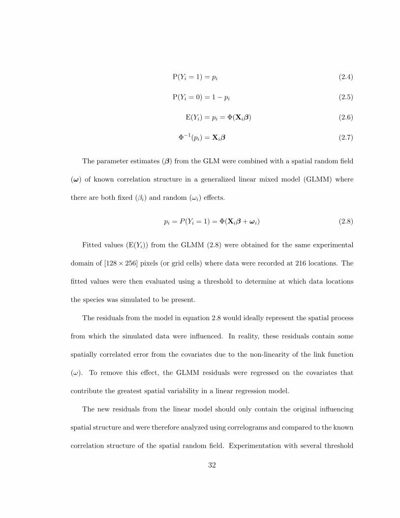
P(Yi = 1) = pi (2.4)

P(Yi = 0) = 1− pi (2.5)

E(Yi) = pi = Φ(Xiβ) (2.6)

Φ−1(pi) = Xiβ (2.7)

The parameter estimates (β) from the GLM were combined with a spatial random field

(ω) of known correlation structure in a generalized linear mixed model (GLMM) where

there are both fixed (βi) and random (ωi) effects.

pi = P (Yi = 1) = Φ(Xiβ + ωi) (2.8)

Fitted values (E(Yi)) from the GLMM (2.8) were obtained for the same experimental

domain of [128× 256] pixels (or grid cells) where data were recorded at 216 locations. The

fitted values were then evaluated using a threshold to determine at which data locations

the species was simulated to be present.

The residuals from the model in equation 2.8 would ideally represent the spatial process

from which the simulated data were influenced. In reality, these residuals contain some

spatially correlated error from the covariates due to the non-linearity of the link function

(ω). To remove this effect, the GLMM residuals were regressed on the covariates that

contribute the greatest spatial variability in a linear regression model.

The new residuals from the linear model should only contain the original influencing

spatial structure and were therefore analyzed using correlograms and compared to the known

correlation structure of the spatial random field. Experimentation with several threshold

32

values was conducted to assess the effects of threshold on simulated residual correlation

structure.

Performing the suggested analysis on simulated data with a known correlation structure

may provide an estimate of the variability in the correlation models for the actual data as

well as provide some insight as to whether or not this process of analyzing residual spatial

structure is appropriate.

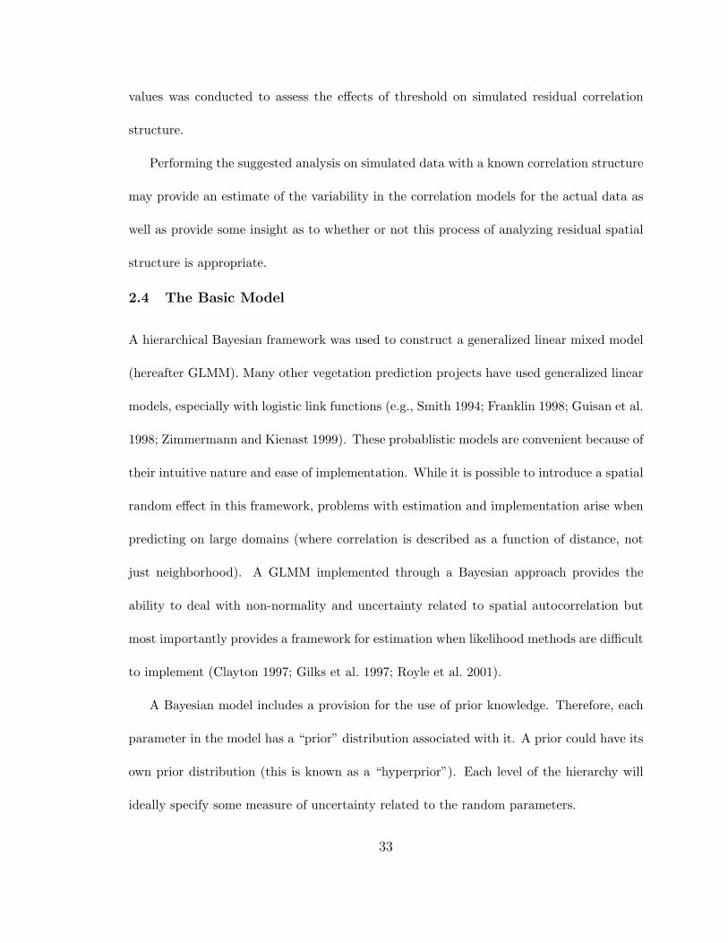
2.4 The Basic Model

A hierarchical Bayesian framework was used to construct a generalized linear mixed model

(hereafter GLMM). Many other vegetation prediction projects have used generalized linear

models, especially with logistic link functions (e.g., Smith 1994; Franklin 1998; Guisan et al.

1998; Zimmermann and Kienast 1999). These probablistic models are convenient because of

their intuitive nature and ease of implementation. While it is possible to introduce a spatial

random effect in this framework, problems with estimation and implementation arise when

predicting on large domains (where correlation is described as a function of distance, not

just neighborhood). A GLMM implemented through a Bayesian approach provides the

ability to deal with non-normality and uncertainty related to spatial autocorrelation but

most importantly provides a framework for estimation when likelihood methods are difficult

to implement (Clayton 1997; Gilks et al. 1997; Royle et al. 2001).

A Bayesian model includes a provision for the use of prior knowledge. Therefore, each

parameter in the model has a “prior” distribution associated with it. A prior could have its

own prior distribution (this is known as a “hyperprior”). Each level of the hierarchy will

ideally specify some measure of uncertainty related to the random parameters.

33

Bayes’ theorem (Equation 2.9) provides a way to combine the distributions from the

data model and the prior model while weighting each accordingly using rules of formal

conditional probability. This combination results in the posterior distribution, of which

there are conditional forms.

P (Bj |A) =P (A|Bj)P (Bj)k∑

i=1

P (A|Bi)P (Bi)

, (Bayes’ Theorem) (2.9)

The real benefit of Bayes’ theorem is that it allows the updating of specified prior beliefs

about a given phenomenon based on the collected scientific data. The resulting posterior

distribution will include information from both models. Mathematically the distributions

can be generalized as:

1.) Data: random variable z whose distribution depends on unknown parameter(s) θ:

z|θ ∼ [z|θ]

(where “ ∼ ” = “is distributed as”, and [z|θ] = “likelihood function”)

2.) Prior Information: (from past data, experts, science, . . . )

θ ∼ [θ]

3.) Posterior: updates the prior belief based on data:

[θ|z] =[z|θ][θ]∫[z|θ][θ]dθ =

[z|θ][θ][z]

A posterior distribution with only one variable can be written as above, however several

variables require the modeling of a joint distribution and become more complex. Many

34

times the posterior distribution of simple models can be worked out analytically. In cases

where the posterior is intractable (as with most complex problems in ecology), a Monte

Carlo method of sampling from the distribution must be used.

2.4.1 MCMC and Gibbs Sampling

Markov Chain Monte Carlo (MCMC) methods have made the implementation of complex

statistical modeling possible through iterative sampling methods (Gilks et al. 1997). MCMC

is not entirely a Bayesian concept, however it lends itself to Bayesian modeling because hier-

archical posterior distributions are usually analytically intractable (Hastings 1970; Clayton

1997; Huffer and Wu 1998).

Specifically, MCMC sampling approaches are used to estimate features of a posterior

distribution by:

1.) Formulating a Markov chain whose stationary distribution coincides with the poste-

rior distribution.

2.) Simulating from said posterior distribution.

Consider the joint distribution of several variables, say w1, . . . ,wk; namely, [w1, . . . ,wk].

Assume that [w1, . . . ,wk] is:

1.) Too complex to implement mathematical formulas to find the normalizing constant

or to find marginal distributions of selected variables.

2.) Too complex to simulate from directly.

35

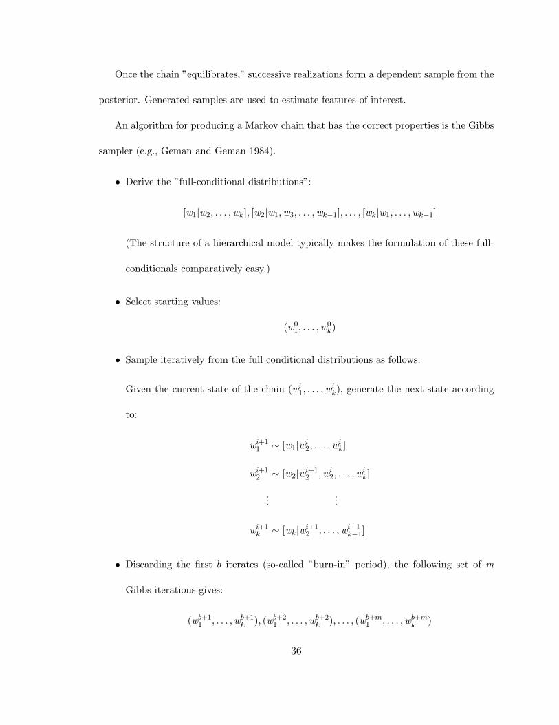
Once the chain ”equilibrates,” successive realizations form a dependent sample from the

posterior. Generated samples are used to estimate features of interest.

An algorithm for producing a Markov chain that has the correct properties is the Gibbs

sampler (e.g., Geman and Geman 1984).

• Derive the ”full-conditional distributions”:

[w1|w2, . . . ,wk], [w2|w1,w3, . . . ,wk−1], . . . , [wk|w1, . . . ,wk−1]

(The structure of a hierarchical model typically makes the formulation of these full-

conditionals comparatively easy.)

• Select starting values:

(w01, . . . ,w

0k)

• Sample iteratively from the full conditional distributions as follows:

Given the current state of the chain (wi1, . . . ,wik), generate the next state according

to:

wi+11 ∼ [w1|wi2, . . . ,wik]

wi+12 ∼ [w2|wi+1

2 ,wi2, . . . ,wik]

......

wi+1k ∼ [wk|wi+1

2 , . . . ,wi+1k−1]

• Discarding the first b iterates (so-called ”burn-in” period), the following set of m

Gibbs iterations gives:

(wb+11 , . . . ,wb+1

k ), (wb+21 , . . . ,wb+2

k ), . . . , (wb+m1 , . . . ,wb+mk )

36

• MCMC estimation approaches (known as ”output analysis,” Ripley (1987)) are ap-

plied to this sample to obtain estimates.

While theory implies that the Markov chain is guaranteed to converge to the appropriate

stationary distribution, implementation issues arise in practice. For example, choices have

to be made to choose starting values and the values of b and m. These issues are still the

focus of ongoing research (e.g., see Gilks et al. 1997).

2.4.2 Hierarchical Linear Regression

Perhaps the simplest way to conceptualize a regression-based model using a Bayesian frame-

work is as follows:

Consider the model:

y = Xβ + ε , where, ε ∼ N(0,Σε) (2.10)

β = Xβα+ η , where, η ∼ N(0,Ση) (2.11)

α = α0 + γ , where, γ ∼ N(0,Σγ) (2.12)

This can be written in distributional notation:

y|X,β,Σε ∼N(Xβ,Σε) likelihood (2.13)

β|Xβ,α,Ση∼N(Xβα,Ση) prior (2.14)

α|α0,Σγ ∼N(α0,Σγ) hyperprior (2.15)

Here it is assumed that Σε,Ση,Σα, and α0 are known parameters. In practice each of

these parameters would have an associated distribution, making them random as well. This

37

multi-tiered structure is what constitutes a hierarchical statistical model. The distribution

of interest excluding the known parameters can be written:

[β,α|y] (2.16)

By Bayes’ theorem:

[β,α|y] ∝ [y|β,α][β,α] ∝ [y|β,α][β|α][α] (2.17)

2.4.3 Bayesian Probit Implementation

Albert and Chib (1993) provide a way to implement a Gibbs sampler for a generalized linear

model using a latent process.

Let:

Yi ={

1 if Zi > 0, species is present at spatial location i0 if Zi ≤ 0, species is absent at spatial location i

(2.18)

Where the latent process Zi is

Zi|β ∼ N(X′iβ, 1)

X = matrix of covariates

β = vector of parameters

The use of the latent Z process allows samples to be generated from a continuous

distribution for the binary process. The model without a spatial term can be written as:

pi = P (Yi = 1) = Φ(X′iβ) (2.19)

Where:

Φ = the probit transform (Normal CDF)

38

The prior for the parameter β in equation (2.19) could be specified as:

β ∼ N(β0,Σβ)

Where:

β0 = the prior means for β

Σβ = the prior covariance matrix for β

Through the Bayesian framework, the posterior distribution provides distributions of β

rather than mean and variance available through frequentist estimation procedures (Fig-

ure 8).

39

Figure 8: Graphical illustration of the distributional information available at thepixel-level provided by the posterior distribution.

40

2.5 The Spatial Model

The latent term (Z) in equation (2.18) is the key to introducing a spatial component.

Consider the following:

Let:

Yi ={

1 if Zi > 0, species is present at spatial location i0 if Zi ≤ 0, species is absent at spatial location i

(2.20)

Where:

Zi ∼ N(X′iβ + ηi, 1) (2.21)

Yi are independent Bernoulli random variables with:

pi = P (Yi = 1) = Φ(X′iβ + ηi) (2.22)

Where:

η = Ψα (2.23)

and

Ψ = some known matrix of spectral basis functions (i.e., Fourier basis functions)

Let the priors be:

β ∼ N(β0,Σβ)

α ∼ N(α0, Dσ2α)

σ2α ∼ IG(qα, rα)

Where:

IG = Inverse Gamma Distribution

D = diag(d1, · · · , dn), the diagonal of a covariance matrix (i.e. the variances)

41

Specifying Inverse Gamma distributions for prior variance parameters is one way to

insure that these will be non-negative. This is critical because variances must be non-

negative.

The full conditionals for the α and β parameters from the posterior distribution can be

written:

β |· ∼ N [(X ′X + Σ−1β )−1((Z− η)′X + β′0Σ−1

β )′, (X ′X + Σ−1β )−1] (2.24)

α |· ∼ N [(Ψ′Ψ +1σ2α

D−1)−1((Z−Xβ)′Ψ +α′0D−1

σ2α

), (I +1σ2α

D−1)−1] (2.25)

Where:

“ |· ” = “given all other parameters”

2.6 Coding the Model

Mechanically, the process of iterative sampling from the posterior distribution is laborious,

therefore computational efficiency is critical in implementing such a model. A programming

language with spectral-transform capabilities and sparse matrix storage running on a dual-

processor computer with large memory was used to perform most of the intensive operations.

Efficient software, fast processors and disk space are not enough to implement the models

proposed here. Therefore, the need for a mathematically efficient algorithm is the key for

including a valid spatial component using large data sets over extensive prediction domains

([256× 128] or 32,768 prediction locations).

2.6.1 Formulation of the Spatial Component

In the model considered here, η (equation 2.23) represents a spatial parameter that may

be related to unknown spatially varying covariates. η is represented as an n × 1 vector of

42

the z-process at the prediction locations. A spectral transformation (Ψ) is the component

that allows for efficient operation of the algorithm in this case. Ψ is an [n × p] matrix of

orthogonal spectral basis functions with the prior, α, acting as spectral coefficients. The

fact that Ψ′Ψ = I (where I is the identity matrix) and D is diagonal allows for a very fast

operation on η by simplifying the full conditionals. This is the step that ultimately makes

it possible to predict on large domains.

The spectral basis functions could be found any of several different ways. In this case a

Fast Fourier Transform on the vector α is sufficient, however methods such as the Discrete

Cosine Transform and Wavelets have been proposed (e.g. Royle and Wikle 2001; Wikle

2001).

Exploratory analysis through simulation experiments showed that predictions may be

especially sensitive to the spatial prior. This emphasizes the need for an extensive prelimi-

nary spatial analysis (Section 2.3.3) as well as the provision for a partially empirical-based

prior to be formed.

2.7 Validation Methods

Validation is critical in a hierarchical modeling project because the complexity of a Bayesian

approach makes it more difficult to get statistical goodness-of-fit measures. Most sample-

space statistics such as p-values and R2 estimates of model fit do not make sense from

a Bayesian perspective. Therefore, innovative methods must be devised to evaluate the

effectiveness of a hierarchical model.

Neter et al. (1996) mention that there are three conventional ways to validate a regression

model.

43

1.) Collection of new data to check the model and its predictive ability.

2.) Comparison of results with theoretical expectations, earlier empirical results, and

simulation results.

3.) Use of holdout sample to check the model and its predictive ability.

Ideally, one would want to use a seperate but temporally similar data set for assessing

the predictive power of the model at locations where data were not originally present. This

would be especially helpful since this project is aimed at predicting continuously across a

spatial domain. Independent data sets are available for selected MOFEP regions, however

the prediction grid chosen for this project does not encompass such regions. It is not

feasible to collect another dataset because the presence of vegetation has been affected by

temporal variability and disturbance from management practices. Therefore, comparison

of predictions with independent data is not an option for model validation.

The comparison of results with theoretical expectations offers promising insight into

realistic natural processes and this will be discussed in chapter 4. The comparison of

results with earlier empirical results is not a validation option for reasons mentioned above.

While comparison with simulation results offered theoretical justification for implementing

a spatial component within the model, it is not a direct validation of the predictions.

The most promising method for model validation suggested by Neter et al. (1996) may

be number three above. By withholding a portion of the original data, the results could

be validated by the randomly withheld sample. In a dataset with only 216 observations,

it is difficult to get a sufficiently large sample to be effective in assessing model accuracy.

44

However, the dataset can be iteratively split into two sets, a model-building set and a

validation or prediction set (this method is known as cross-validation), for a series of model

runs. Upon each iteration the validation set is compared with the predictions gained from

modeling with the model-building set. The comparisons are reported in contingency tables

and also the independence in predicted probabilities given the true data was tested for

significance with a chi-squared test. Zar (1984) provides the following formulation of a χ2

test statistic:

χ2 =n(|f1,1f2,2 − f1,2f21| − n

2 )2

(C1)(C2)(R1)(R2)(2.26)

Where the following contigency table exists:

PredictedP A total

RealP f1,1 f1,2 R1

A f2,1 f2,2 R2

total C1 C2 n

The use of such a test assumes a null hypothesis of: The predicted occurrence of a

species is independent of the true occurrence of a species. The alternate hypothesis is: The

predicted occurrence of a species is associated with the true occurrence of a species. Chi-

squared tests are commonly used for assessing the accuracy of binary regression models. It

is important to note that such tests applied in similar situations are subject to threshold

values and although informative, may not provide adequate validation for models of this

type. Chi-squared tests in conjunction with the boxplots for predicted probabilities versus

real occurrence can be used to suggest that a given threshold is reasonable.

45

The primary benefit of using a rigorous statistical approach to modeling is the ability to

use a model-based validation. In this hierarchical framework each parameter is modeled on

a pixel by pixel basis resulting in a distribution for each grid cell (Figure 8). Just as a pixel

mean can be reported by averaging the posterior predictions for parameters of interest, a

measure of error about the mean (standard deviation or variance) can be reported as well.

It follows that these measures can be presented in the form of an image and would represent

the spatial distribution of prediction error on the domain. Such images provide a reasonable

means with which to evaluate model accuracy and add to the overall validation of the model

(Royle et al. 2001).

46

3 RESULTS

3.1 Exploratory Results

3.1.1 Field Data / Covariate Preliminary Analysis

The results of the field data/covariate analysis can be illustrated graphically. Barplots have

been used to show the effect of categorical covariates on species occurrence while boxplots

have been used to show the effect of continuous covariates.

The response of Desmodium glutinosum and Desmodium nudiflorum to the Land Type

Association covariate is evident in Figure 9. Desmodium glutinosum occurs in the Current

River Oak Forest Breaks (LTA 2) slightly more than the Current River Oak-Pine Wood-

land/Forest Hills (LTA 4) in the prediction domain. Conversely, Desmodium nudiflorum

seems to occur more in the hills than the breaks.

The barplots suggest that variable depth soil may be a stronger influence than Land

Type Association on where these species will grow. Although only 12 subplots fall within

variable depth soil areas, the percent of subplots where each species was present to the total

number of subplots in that category shows that both species are more common on variable

depth soils (Figure 9).

It is important to remember that just because the relationship is not perfectly evident

in these simple graphs does not mean there is not some more complex process involving

Ecological Land Type or Land Type Association that influences this species. For instance,

if the response of vegetation to ELT or LTA is altered by some unknown non-linear or

multi-modal process (such as herbivory or micro-climate) the relationships illustrated with

barplots may not accurately portray the true response.

47

The SWNESS covariate is likely the strongest known factor influencing species occur-

rence. The differentiation between presence and absence for both species across aspects is

evident in Figure 10. The subplots where Desmodium glutinosum and Desmodium nudiflo-

rum were present show much higher densities at the Northeast aspect than the Southwest.

Additionally, there are few occurrences at Southeast and Northwest aspects, suggesting that

this covariate is a reasonable transformation of aspect when modeling these species.

Relative elevation as a covariate shows some differentiation between those subplots where

Desmodium glutinosum was present and where it was absent. The plot in Figure 11 suggests

that slighly lower elevations positively influence the occurrence of this plant. Desmodium

nudiflorum, on the other hand, exhibits little differentiation between high and low elevations

and shows no separation in confidence intervals. Therefore, this covariate is expected to

account for minimal variability when modeling the environmental influences of Desmodium

nudiflorum but may be important for Desmodium glutinosum.

48

Desmodium nudiflorum Desmodium glutinosum

LTA 2LTA 4

Land Type Association

Species

ratio

of #

pre

sent

to to

tal i

n ca

tego

ry

020

4060

Desmodium nudiflorum Desmodium glutinosum

Variable DepthNot Variable Depth

Variable Depth Soil

Species

ratio

of #

pre

sent

to to

tal i

n ca

tego

ry

020

4060

80

Figure 9: Barplots showing percent of subplots where Desmodium glutinosum andDesmodium nudiflorum are present out of the total number of subplots for eachcategory in the Land Type Association and Variable Depth covariates.

49

present absent

−1.

0−

0.5

0.0

0.5

1.0

Desmodium glutinosum

SW

NE

SS

present absent

−1.

0−

0.5

0.0

0.5

1.0

Desmodium nudiflorum

SW

NE

SS

Figure 10: Boxplots of those subplots where Desmodium glutinosum and Desmodiumnudiflorum were present and absent in terms of the SWNESS variable. A value of 1represents the most Southwest aspect, while a value -1 represents the most Northeastaspect. Box widths are relative to the amount of data within the category and boxnotches represent a 95% confidence interval for the median.

50

present absent

0.2

0.4

0.6

0.8


Rel

ativ

e E

leva

tion

present absent

0.2

0.4

0.6

0.8


Rel

ativ

e E

leva

tion

Figure 11: Boxplots of those subplots where Desmodium glutinosum and Desmodiumnudiflorum were present and absent in terms of the Relative Elevation variable. Avalue of 1 represents the highest elevation in the prediction domain while a value of 0represents the lowest elevation. Box widths are relative to the amount of data withinthe category and box notches represent a 95% confidence interval for the median.

51

3.1.2 Simulation and Preliminary Spatial Analysis

The extensive exploratory data analysis described in Section 2.3.3 is helpful in providing

evidence that may suggest plant occurrence is influenced by some underlying spatial process.

Spatial structure is commonly illustrated using semi-variograms and variograms at noted

in Section 2.3.2. Correlograms standardize the semi-variance and thus are more suited for

comparison of spatial dependence. Spatial dependence can be observed in correlograms as

the rate of change of the correlation. It follows that little or no spatial structure exists

beyond the distance at which the correlation stabilizes (or when the correlation approaches

zero).

Underlying spatial structure influencing the distribution of Desmodium glutinosum and

Desmodium nudiflorum is obtained by the process described in Section 2.3.3, whereby spa-

tial correlation is derived from the residuals of which all covariate effects are removed. The

change in correlation over distance was used to fit an exponential model to the empirical

correlogram (Figures 12, 13).

The distance at which residual spatial structure subsides for Desmodium glutinosum is

less than that for Desmodium nudiflorum. The variability in the data around the fitted

exponential model can be thought of in terms of root mean squared error, and appears to

be similar for both species at approximately 0.08.

Presence/absence data that were influenced by known spatially correlated error were

simulated and the covariate effect was then removed by the same process that was used for

the actual data. Correlation in the residuals of the simulated data was compared with four

different levels of known correlation structure from which the data were informed. These

52

correlograms are depicted in Figures 14, 15, 16, and 17.

The estimated spatial structure is influenced by sampling variability, therefore the cor-

relation must be estimated through multiple simulations. 500 spatial random fields were

simulated at different levels of theta (θ =3, 5, 7, and 9) to get an estimate of the residual

structure. This series of parameterizations was chosen because it encompassed the sus-

pected parameter estimates for the two species of interest. Lower values of θ imply a more

localized spatial effect.

At each level of structure the exponential model fit the original structure of the ran-

dom field quite well with the root mean squared error consistently less than 0.02. The

correlograms in Figures 12–17 are plotted for distances from 0–100 pixels (0–1000 meters)

although the data extend beyond that range.

53

0 20 40 60 80 100

−0.2

0.0

0.2

0.4

0.6

0.8

1.0

Correlogram for Desmodium glutinosum

distance

corr

elat

ion

EmpiricalFitted

theta=5.3695

RMSE=0.08255

Figure 12: The empirical correlogram for Desmodium glutinosum and its exponen-tially fitted counterpart with parameter theta and RMSE being the root mean squarederror of the fitted model. Distance is in grid cells (1 pixel = 10 meters)

54

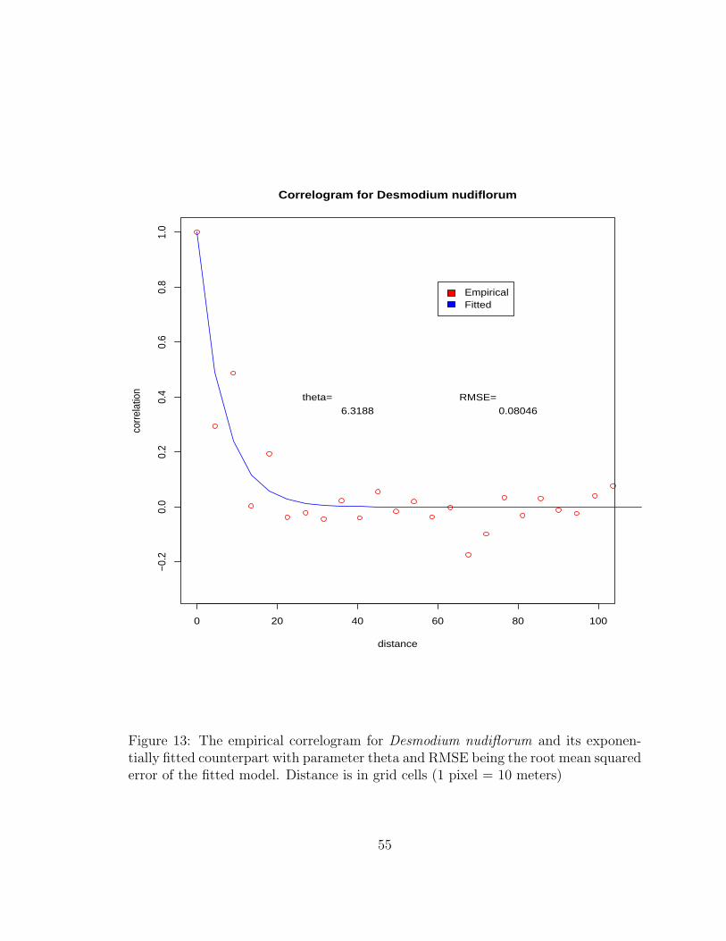
0 20 40 60 80 100

−0.2

0.0

0.2

0.4

0.6

0.8

1.0

Correlogram for Desmodium nudiflorum

distance

corr

elat

ion

EmpiricalFitted

theta=6.3188

RMSE=0.08046

Figure 13: The empirical correlogram for Desmodium nudiflorum and its exponen-tially fitted counterpart with parameter theta and RMSE being the root mean squarederror of the fitted model. Distance is in grid cells (1 pixel = 10 meters)

55

0 20 40 60 80 100

−0.2

0.0

0.2

0.4

0.6

0.8

1.0

Correlogram for Simulated Data

distance

corr

elat

ion

RealEmpiricalFitted

real theta=3

fitted theta=3.22

empirical RMSE=

0.02286fitted RMSE=

0.003519

Figure 14: The correlogram created using data informed from a known model withparameter theta (real theta = 3) and the resulting empirical and exponentially fittedcounterparts with parameter theta (fitted theta) and RMSE being the root meansquared error of the empirical correlogram and fitted model. Distance is in grid cells(1 pixel = 10 meters)

56

0 20 40 60 80 100

−0.2

0.0

0.2

0.4

0.6

0.8

1.0


distance

corr

elat

ion

RealEmpiricalFitted

real theta=5

fitted theta=5.772

empirical RMSE=

0.03425fitted RMSE=

0.01187


57

0 20 40 60 80 100

−0.2

0.0

0.2

0.4

0.6

0.8

1.0


distance

corr

elat

ion

RealEmpiricalFitted

real theta=7

fitted theta=7.364

empirical RMSE=

0.02543fitted RMSE=

0.005019


58

0 20 40 60 80 100

−0.2

0.0

0.2

0.4

0.6

0.8

1.0


distance

corr

elat

ion

RealEmpiricalFitted

real theta=9

fitted theta=9.227

empirical RMSE=

0.03022fitted RMSE=

0.002812


59

3.2 Modeling Results

An area within sites 1 and 2 (Figure 1) consisting of nearly 330 hectares (≈33,000 grid cells)

was chosen to test the model. Of the 2592 MOFEP subplots, 216 fall within the aforemen-

tioned area (see Figure 3) and these are utilized in this form of the model. Approximately

32% of the data locations contained Desmodium glutinosum while 74% of the sampled lo-

cations contained Desmodium nudiflorum. The data locations only make up 0.66% of the

prediction grid and are therefore very sparse within prediction domain.

By predicting at a discrete and contiguous number of locations (grid cells in this case)

over a continuous spatial domain, maps that display information about the posterior dis-

tribution can be created. Maps based on predicting the E(Yi) process, such as those shown

in this section, can be viewed as probabilistic maps of species occurrence, such that map

intensities can range from 0 to 1 (1 being 100% probability of species occurrence).

The Gibbs sampler was run for 10,000 iterations and a burn-in period of 2000 iter-

ations was used to insure model convergence. Resulting parameter distributions can be

summarized in the form of histograms. Figures 18 and 19 show the marginal posterior

distributions for the parameters, β, in equation 2.25 for both species. It can be inferred

that the covariates are indeed important factors influencing the occurrence of these species

because the distributions for β generally do not overlap zero. In the case of Land Type As-

sociation for Desmodium glutinosum, a slight overlap of zero is evident. This suggests that

the Land Type Association covariate accounts for less variability than the other covariates

when modeling this species.

If no known covariates exist, the process could be modeled solely as a spatial random

60

field over the prediction domain. This process would be influenced only by the relative

geographic location of the data points (Figures 20 and 26). By withholding covariates from

the proposed model, the posterior prediction for the η–process represents a sole spatial

random field for the data. The mean image for this field would be similar to the outcome

of disjunctive kriging (Cressie 1993) and is illustrated for both species in Figures 21 and 27.

The data locations are marked red and blue, while areas with no data are green. A value

of 1 displays where the species was present, while a value of -1 is where the species was

absent.

The Gibbs sampler also yields posterior means for other model parameters when fit with

covariates (X in equation 2.22), such as the spatial process (η in equation 2.23). Recall

that η corresponds to the residual spatial random effect that ultimately helps the model fit

the real process. This random field can be mapped and may provide valuable insight into

the latent process (Figures 23, 29).

Posterior prediction means were obtained from the Gibbs sampler for each unit in the

prediction domain (E(pi) in equation 2.6). These means are re-assembled into an image and

illustrate the expected value for the predicted distribution in each pixel (Figures 22, 28).

Additionally, image realizations can graphically portray the variablilty in pixel distributions

(Figures 24, 25, 30, 31).

61

−0.75 −0.7 −0.65 −0.6 −0.55 −0.50

10

20

30

40

50Southwestness

−3 −2.5 −2 −1.50

10

20

30

40Relative Elevation

−0.5 0 0.5 10

5

10

15

20

25

30

35Land Type Association

0 0.1 0.2 0.3 0.4 0.50

10

20

30

40

50Variable Depth Soil

Mean=−0.6 Mean=−2.13

Mean=0.19 Mean=0.25

Figure 18: Resulting histograms of the β parameters from the posterior distributionfor Desmodium glutinosum.

62

−1.2 −1 −0.8 −0.60

20

40

60

80

100Southwestness

1 1.2 1.4 1.6 1.8 20

10

20

30

40Relative Elevation

0.5 1 1.50

20

40

60

80

100Land Type Association

−2 −1.8 −1.6 −1.4 −1.2 −10

50

100

150

200

250Variable Depth Soil

Mean=−0.83 Mean=1.51

Mean=1.11 Mean=−1.54

Figure 19: Resulting histograms of the β parameters from the posterior distributionfor Desmodium nudiflorum.

63

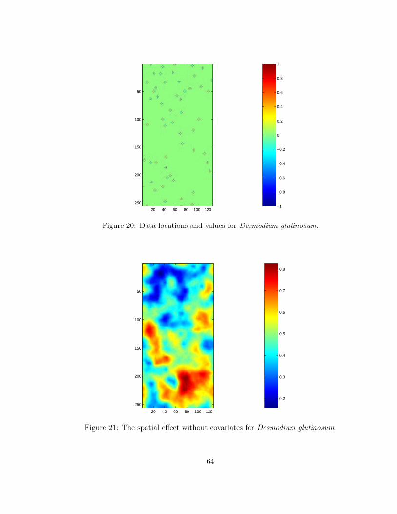
−1

−0.8

−0.6

−0.4

−0.2

0

0.2

0.4

0.6

0.8

1

20 40 60 80 100 120

50

100

150

200

250

Figure 20: Data locations and values for Desmodium glutinosum.

0.2

0.3

0.4

0.5

0.6

0.7

0.8

20 40 60 80 100 120

50

100

150

200

250

Figure 21: The spatial effect without covariates for Desmodium glutinosum.

64

0.1

0.2

0.3

0.4

0.5

0.6

0.7

0.8

20 40 60 80 100 120

50

100

150

200

250

Figure 22: Posterior mean prediction image showing the mean predicted process con-sidering the covariates and residual spatial random effect for Desmodium glutinosum.

65

0.2

0.3

0.4

0.5

0.6

0.7

0.8

20 40 60 80 100 120

50

100

150

200

250

Figure 23: Posterior mean for the η process showing the residual spatial randomeffect for Desmodium glutinosum.

66

0.1

0.2

0.3

0.4

0.5

0.6

0.7

0.8

0.9

20 40 60 80 100 120

50

100

150

200

250

Figure 24: One realization from the posterior distribution of D. glutinosum.

0.1

0.2

0.3

0.4

0.5

0.6

0.7

0.8

0.9

20 40 60 80 100 120

50

100

150

200

250

Figure 25: Another realization from the posterior distribution of D. glutinosum.

67

−1

−0.8

−0.6

−0.4

−0.2

0

0.2

0.4

0.6

0.8

1

20 40 60 80 100 120

50

100

150

200

250

Figure 26: Data locations and values for Desmodium nudiflorum.

0.2

0.3

0.4

0.5

0.6

0.7

0.8

0.9

20 40 60 80 100 120

50

100

150

200

250

Figure 27: The spatial effect without covariates for Desmodium nudiflorum.

68

0.3

0.4

0.5

0.6

0.7

0.8

0.9

20 40 60 80 100 120

50

100

150

200

250

Figure 28: Posterior mean prediction image showing the mean predicted process con-sidering the covariates and residual spatial random effect for Desmodium nudiflorum.

69

0.3

0.35

0.4

0.45

0.5

0.55

0.6

0.65

0.7

0.75

20 40 60 80 100 120

50

100

150

200

250

Figure 29: Posterior mean for the η process showing the residual spatial randomeffect for Desmodium nudiflorum.

70

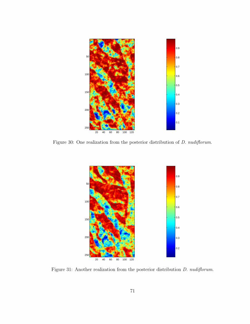
0.1

0.2

0.3

0.4

0.5

0.6

0.7

0.8

0.9

20 40 60 80 100 120

50

100

150

200

250

Figure 30: One realization from the posterior distribution of D. nudiflorum.

0.2

0.3

0.4

0.5

0.6

0.7

0.8

0.9

20 40 60 80 100 120

50

100

150

200

250

Figure 31: Another realization from the posterior distribution D. nudiflorum.

71

3.3 Validation

As mentioned in chapter 2, the validation of a hierarchical statistical model is more difficult

than for a simple linear regression model. Therefore, two primary methods were used for

assessing the model accuracy.

1.) Testing for independence between predicted occurrence and real occurrence using

cross-validation.

2.) Presenting maps of prediction error in the form of marginal posterior standard devi-

ations for pixel means.

A threshold value was used to create binary values from the mean probability images so

that when the probability is greater than the threshold the species is thought to be present

and when it is less than the threshold the species is thought to be absent.

Conventionally, a probability threshold of 0.5 is used, however this may not always

be the most reasonable threshold for these predictions because the data may not encom-

pass the threshold. Determining if the model is distinguishing between those subplots

where the species is present and those where it is absent is sufficient. Therefore chosing

a threshold between the two distributions of predictions is the most reasonable approach.

Boxplots showing the differentiation of predicted probabilities for Desmodium glutinosum

and Desmodium nudiflorum are shown in Figure 32. Such boxplots suggest that a 50%

threshold is a reasonable cutoff for the predicted probabilities in this case.

Approximately 50% of the original data were randomly withheld in an iterative fashion

and the model output was aggregated in order to test for independence as discussed in

72

section 2.7. The two-by-two contingency tables for both species are shown below. Results

from the chi-squared tests are summarized in Table 3.

D. glutinosum PredictedThreshold=0.5 P A total

RealP 18 15 33A 10 57 67

total 28 72 100D. nudiflorum PredictedThreshold=0.5 P A total

RealP 64 7 71A 16 13 13

total 80 20 100

The second part of the validation is based on maps of prediction error presented in

Figures 33 and 34. These maps, created using the marginal posterior standard deviations

for pixel means, offer a rigorous spatially based measure of model accuracy. The results

of such mapping efforts are similar for both species, and show that the prediction error is

greatest at locations farthest from the data.

73

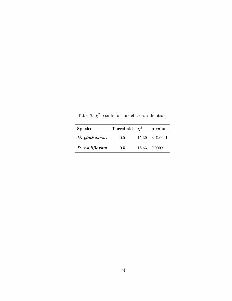
Table 3: χ2 results for model cross-validation.

Species Threshold χ2 p-value

D. glutinosum 0.5 15.30 < 0.0001

D. nudiflorum 0.5 13.63 0.0002

74

present absent

0.0

0.2

0.4

0.6

0.8


real occurrence

pred

icte

d pr

obab

ility

present absent

0.2

0.4

0.6

0.8


real occurrence

pred

icte

d pr

obab

ility

Figure 32: Boxplots showing the differentiation for predicted probabilities by realoccurrence for Desmodium glutinosum and Desmodium nudiflorum. Box widths arerelative to the amount of data within the category and box notches represent a 95%confidence interval for the median.

75

0.05

0.1

0.15

0.2

0.25

20 40 60 80 100 120

50

100

150

200

250

Figure 33: Standard deviation map for the prediction mean of D. glutinosum.

0.05

0.1

0.15

0.2

20 40 60 80 100 120

50

100

150

200

250

Figure 34: Standard deviation map for the prediction mean of D. nudiflorum.

76

4 DISCUSSION

4.1 Exploratory Analysis

The plots in Section 3.1 show that some relationships between the field data and covariates

exist. It was noted that not all relationships were apparent in the figures, but that the vari-

ables may be interacting in a complex manner. This was expected and may be accounted for

in the model because the parameters are allowed to vary randomly according to probability

distributions. It is also important to note that other more influential covariates could easily

be utilized by the model if they were explicitly known on the prediction domain. It is clear

that there are likely more important factors influencing the occurrence of the species.

Variables such as herbivory, seed disperal, micro-climate, inter-species and intra-species

competition were discussed in Section 1.1.5 as potentially influential factors. It is difficult

to gain explicit knowledge about such factors over large spatial domains. The only hope of

accounting for uncertainty these factors may contribute is through identifying and quantify-

ing a latent spatial random field that mimics the effect of one or more unknown covariates.

Once this random field can be parameterized and defined by a model it will aid a species

or habitat prediction model by accounting for otherwise inaccessible uncertainty.

Determining the appropriate underlying spatial random effect (as in Figures 12 and 13)

is an essential part of this project because it is the spatial component of the proposed model

that is unique to this project. A simple generalized linear model would be sufficient for this

project if the underlying spatial process contains no dependence.

The simulations performed and illustrated in Figures 14, 15, 16, and 17 are the key to

justifying why this process of analyzing spatial dependence is reasonable. By simulating

77

data (at the same locations as the actual data) with the covariates and a known spatial

random effect, the process described in Section 2.3.3 can be tested to insure that it is indeed

identifying the actual underlying spatial structure. Figures 14, 15, 16, and 17 show that the

residual correlation is quite similar to the correlation from which the data were informed,

therefore using the same methodology to evaluate the actual data is expected to provide an

approximation of the underlying spatial structure with a minimal amount of error.

The variability in the empirical correlation around the fitted correlogram for the actual

data is expected and likely due to some unknown random process. This variability is reduced

in the correlograms for the simulated data because of the controlled nature of the explicitly

informed data.

4.2 The Model

Results of the modeling were both expected and unexpected, but informative nonetheless.

A pattern of spatial arrangement in the raw data was evident and expected. As mentioned,

this is likely due to the effect of influential spatial processes in environmental covariates.

However if none of these covariates are explicitly known on the domain, a pure spatial

prediction could be gained from the geographic location and value of the data alone.

Patterning in the predicted images for the posterior mean of the raw spatial process

somewhat resembled that of the images for covariate-based predicted means. This similarity

occurs because the raw spatial process is trying to absorb any spatial correlation in the

unknown covariates. Differences between the two predictions illustrate the need for spatially

explicit covariates in the model.

In the event that covariates are known, a residual spatial process (as discussed in the

78

previous section) may help inform the model. In this case, the level of correlation in such a

process can be estimated a priori and used as a prior in the proposed hierarchical model.

In practice, this can also be used to inform the starting values for the Markov chain and

will help the model converge more rapidly. Informing priors from the data is an empirical

Bayesian view and not shared by all Bayesians, however it is practical because it usually

speeds model convergence.

The modeled residual spatial random field (η) given in Figures 23 and 29 can be thought

of as the “missing covariate(s)” and will ultimately improve the accuracy of the model.

Images given in Figures 23 and 29 illustrate that the η-process differs by species as suggested

in the exploratory analysis (Figures 12 and 13). From an analytical standpoint, it is clear

that the process is most evident in neighborhoods about the data. From an ecological

standpoint, these neighborhoods likely have an implicit biological meaning. The evaluation

and interpretation of a given species η-process could be extensive and is therefore beyond

the scope of this project. It is recognized however, that the residual process is probably a

synthesis of complex interactions, both biological and environmental.

The predicted mean images for each plant graphically depict relationships between the

vegetation and environment (Figures 22 and 28). Mathematically, the pixel intensities of

such maps are based on fully rigorous relationships and represent the best possible quality

predictions available. Ecologically, the predictions are based on a combination of envi-

ronmental factors and surrogates for biological factors, making them a very complete and

robust reflection of the species response on a continuous spatial domain. Theoretically, this

response might be interpreted as the spatial prediction of vegetation occurence or perhaps

79

suitable habitat. It is suggested that the interpretation be flexible so it may individually

suit a specific project.

Predicted maps of the mean posterior probabilities take the form of the covariates.

Therefore the predicted images (represented by a grid) could be utilized in a GIS for an

endless number of applications. Additionally, output from the proposed model could be used

as covariates in another model (such as a model predicting wildlife habitat, fire susceptibility,

forage, . . . ). Importantly, measures of uncertainty related to these covariates are would then

be available (such information has traditionally been unavailable).

Recall that with a Hierarchical Bayesian approach, model parameters are assumed to

follow some random distribution. Taking this into consideration, the most intuitive way

to visualize the posterior distribution may be a map of mean predictions. The quality

of the model output allows for a much deeper conceptualization of the predictions. If a

process is considered random, then at any given time at any given location, the response is

expected to follow some distribution. In reality, the response at a given time and location

is represented by a single value. In the scope of this project that value is the probability

of a certain species being present. This value is a realization of that random process. If

a realization is taken from each pixel distribution on a contiguous domain, the result is

a map of realizations (or a realization map of the process). Such a map, as presented in

Figures 24, 25, 30 and 31 can be thought of as a snapshot of a stochastic process. These

maps offer little in the way of utility for other predictive projects, but have much to offer

as foundations for theoretical projects investigating patch dynamics, realistic vegetation

patterning, or environmental simulation.

80

4.3 Validation

According to Levins (1966):

A mathematical model is neither an hypothesis nor a theory. Unlike scientific

hypotheses, a model is not verifiable directly by an experiment. For all models

are both true and false. . . . The validation of a model is not that it is “true”

but that it generates good testable hypotheses relevant to important problems.

A model may be discarded in favor of a more powerful one, but it usually is

simply outgrown when the live issues are not any longer those for which it

was designed. . . . The multiplicity of models is imposed by the contradictory

demands of a complex, heterogeneous nature and a mind that can only cope

with a few variables at a time . . . individual models, while they are essential for

understanding reality, should not be confused with that reality itself.

In the case of the model proposed here, the concern is not as focused on validation as it

is on methodology. Levins remarks are directed at those models that were designed with a

specific utility in mind. The purpose of this project is to provide methods that are robust

enough to be applied to a number of different applications. Of course a specific scenario

was chosen to test and present the proposed methods and as such the validation of this

model applied to the specific scenario has the purpose of illustrating certain advantages of

the technique.

The chi-squared tests provided a way to evaluate the ability of the model to distinguish

between those areas where a species should be present or absent. The tabular results of the

81

tests showed that the specified threshold of 0.5 is a reasonable classification criteria for these

data. However, as mentioned earlier, statistics that are dependent on such analyst-based

classifications are subjective but not entirely meaningless. They still provide a way to test

the differentiating power of the model. Chi-squared tests used here prove that the model is

distinguishing between presence and absence for both species. Resulting p-values allow the

rejection of a null hypothesis that predictions and actual data are independent.

It was mentioned earlier that one advantage of using a statistical model over a more

ad hoc approach, is the ability to provide a model-based estimate of prediction error. In

a spatial setting this information is especially valuable for it can provide an error estimate

at each prediction location. In the form of a map, this information can be compared

to the location of field data, covariate effects, residual spatial effects, and ultimately the

predictions. The practice of reporting error for spatially explicit data is becoming more

popular (e.g. Justice and Running 1998) and it is convenient that the approach presented

here automatically provides a way to incorporate such information.

It is common for maps of marginal posterior standard deviations to illustrate that the

model (usually hierarchical) is good at predicting near the locations of the actual data,

and gains some error as it is applied further from the data (Royle et al. 2001). The maps

presented in Figures 33 and 34 illustrate this expected patterning of prediction error. Over-

all, the standard deviations of the posterior mean predictions are quite small and suggest

that the model is doing a good job predicting occurrence for both species (especially near

the locations of the data). This accuracy is no doubt due to the hierarchical nature of

the model because it accounts for several levels of uncertainty including a spatial random

82

effect. Such maps have the potential to be quite useful in other hierarchical models where

it is appropriate to specify uncertainty related to prior information. Ultimately this chain

of utilizing the output from hierarchical models for the formulation of priors or data in new

models could prove to be useful in modeling more complex systems.

83

5 CONCLUSIONS

The purpose of this project was to develop and test a robust methodology for realistically

modeling natural processes at a landscape level. Specifically, this problem was considered

from a hierarchical Bayesian perspective. This approach has allowed the incorporation of a

critical spatial component into a generalized linear mixed model. Similar modeling method-

ologies have been proposed, however many are currently focused on small spatial domains

because of mathematical and computational limitations. The formulations presented here

are aimed at predicting natural processes on larger domains.

Advancements in GPS (global postitioning system) technologies have allowed for im-

proved field data collection methods and hence improvement of designed experiments. Sim-

ilarly, the progress in GIS (geographic information systems) technology has made spatially-

explicit environmental information available on large contiguous domains. The combination

of these features opens many doors for the development of new statistical procedures as well

as new ways to answer questions about complex associations between biological and envi-

ronmental systems.

The methodology presented in Chapter Two was tested using part of a landscape level

dataset collected in the Missouri Ozarks as part of the Missouri Ozark Forest Ecosystem

Project. Relationships between vegetation occurrence and known environmental features

were investigated in an exploratory analysis. Residual spatial random effects in the data

were observed and extensively analyzed via several methods. Simulations were conducted

to insure that the proposed methods of informing a spatial prior were indeed reasonable.

An approach for constructing generalized linear models was modified to include a spatial

84

parameter. The coding of this model was optimized using a spectral transformation that in-

variably simplified the formulation of the marginal posterior distributions. The integrations

required to analytically find the necessary joint distributions were intractible, therefore the

model was implemented using an iterative process known as Markov Chain Monte Carlo

that allowed samples to be drawn from the posterior distribution through a Gibbs sampler.

Parameter distributions, mean prediction images, maps of the residual spatial process,

and realizations were provided in order to show the range of information available through

this approach. Different methods for validating such models were presented and applied to

the modeling results for Desmodium glutinosum and Desmodium nudiflorum. Both valida-

tion methods suggested that this model is performing quite well overall and is especially

accurate at predicting near the original data.

As mentioned earlier, probabilistic results of the proposed model using the example

dataset could be viewed as the spatial prediction of a species on a continuous domain at the

time of data collection or as the realized niche of the given species. It was not the intent

of the project to determine which description is most appropriate but to provide the most

robust and informative predictions about the ecological process.

The information provided by the proposed model represents a recognized need by many

researchers in all natural resource fields. However, previous attempts to provide landscape-

level information about biological systems have met with resistance due to their lack of rigor,

extent, applicability, and theoretical implications. The problem of dealing appropriately

with spatially correlated data has become increasingly recognized as an important topic in

ecology during the past decade. A method for recognizing and utilizing spatial dependence

85

in ecological data has been presented here.

In conclusion, this document has provided a detailed description of a methodology for

spatially modeling natural processes on large spatial domains within a rigorous statistical

framework. This technique was implemented using local data and provided ecologically

interesting results that were validated with two different approaches which proved to verify

the accuracy of the proposed model.

Finally, a relevant quote from Box (1976) reads: “All models are wrong, some are use-

ful.” Given that a model is always wrong, it may become useful if the degree to which

it is wrong is known. Realizing that the modeling methodology presented in this project

could never perfectly represent a true ecological process, it is hoped that it may find ap-

plication in a variety of disciplines where the analyst will make use of the extraordinarily

rich qualitative and quantitative information it provides. The most promising applications

of this methodology range from the utilization of posterior prediction maps as covariates in

more complex models to inference about the dynamics of spatial community structure in

vegetation.

86

LITERATURE CITED

Agnew, A., J. Wilson, and M. Sykes. 1993. A vegetation switch as the cause of a forest/mireecotone in New Zealand. Journal of Vegetation Science, 4:273–278.

Albert, J. and S. Chib. 1993. Bayesian analysis of binary and polychotomous responsedata. Journal of the American Statistical Association, 88(422):669–679.

Allen, T. and T. Starr. 1982. Hierarchy. University of Chicago Press, Chicago, Illinois.

Augustin, N., M. Mugglestone, and S. Buckland. 1998. The role of simulation in modelingspatially correlated data. Environmetrics, 9:175–196.

Austin, M. Perspectives in Plant Competition, chapter Community theory and competitionin vegetation. Academic Press, New York, New York, USA, 1990.

Austin, M., A. Nichols, and C. Margueles. 1990. Measurement of the realized qualitativeniche: environmental niches of five eucalyptus species. Ecological Monographs, 60:161–177.

Austin, M. and T. Smith. 1989. A new model for the continuum concept. Vegetatio, 83:35–47.

Beatty, S. 1984. Influence of microtopography and canopy species on spatial patterns offorest understory plants. Ecology, 65(5):1406–1419.

Beers, T., P. Dress, and L. Wensel. 1966. Aspect transformation in site productivityresearch. Journal of Forestry, 64:691–692.

Besag, J. 1972. Nearest-neighbor systems and the auto-logistic model for binary data.Journal of the Royal Statistics Society, 36:75–83.

Besag, J. 1974. Spatial interaction and the statistical analysis of lattice systems. Journalof the Royal Statistics Society, 36:192–236.

Borcard, D., P. Legendre, and P. Drapeau. 1992. Partialling out the spatial component ofecological variation. Ecology, 73:1045–1055.

Box, G. 1976. Science and Statistics. Journal of the American Statistical Association, 71:791–799.

Bridge, S. and E. Johnson. 2000. Geomorphic principles of terrain organization and vege-tation gradients. Journal of Vegetation Science, 11:57–70.

Brookshire, B. and D. Dey. Establishment and data collection of vegetation-related studieson the Missouri Ozark Forest Ecosystem Project study sites. In Brookshire, B. and S.Shifley, editors, Missouri Ozark Forest Ecosystem Project: site history, soils, landforms,woody and herbaceous vegetation, down wood, and inventory methods for the landscape ex-periment, number GTR NC-208, pages 1–18, St. Paul, Minnesota, 2000. U.S. Departmentof Agriculture, Forest Service, North Central Forest Experiment Station.

87

Brookshire, B., R. Jensen, and D. Dey. The Missouri Ozark Forest Ecosystem Project: past,present, and future. In Brookshire, B. and S. Shifley, editors, Proceedings of the MissouriOzark Forest Ecosystem Project symposium: an experimental approach to landscape re-search, number GTR NC-193, pages 1–25, St. Paul, Minnesota, 1997. U.S. Departmentof Agriculture, Forest Service, North Central Forest Experiment Station.

Brown, D. 1994. Predicting vegetation types at treeline using topography and biophysicaldisturbance variables. Journal of Vegetation Science, 5:641–656.

Brzeziecki, B., F. Kienast, and O. Wildi. 1993. A simulated map of the potential naturalforest vegetation of Switzerland. Journal of Vegetation Science, 4:499–508.

Carlin, B. and T. Louis. 2000. Bayes and Empirical Bayes Methods for Data Analysis.Chapman & Hall, Boca Raton, Florida.

Cherrill, A., C. McClean, P. Watson, K. Tucker, S. Rushton, and R. Sanderson. 1995.Predicting the distributions of plant species at the regional scale: A hierarchical matrixmodel. Landscape Ecology, 10:197–207.

Clark, J., S. Carpenter, M. Barber, S. Collins, A. Dobson, J. Foley, D. Lodge, M. Pascual,R. Pielke Jr., W. Pizer, C. Pringle, W. Reid, K. Rose, O. Sala, W. Schlesinger, D. Wall,and D. Wear. 2001. Ecological Forecasts: An emerging imperative. Science, 293(5530):657–660.

Clayton, D. Markov Chain Monte Carlo in Practice, chapter 16, Generalized linear mixedmodels, pages 276–301. Chapman & Hall, New York, New York, 1997.

Clements, F. 1936. Nature and structure of the climax. Journal of Ecology, 24:252–284.

Cliff, A. and J. Ord. 1972. Testing for spatial autocorrelation among regression residuals.Geographical Analysis, 4:267–284.

Cliff, A. and J. Ord. 1981. Spatial Processes: models and applications. Pion, London,England.

Collins, S., S. Glenn, and D. Roberts. 1993. The hierarchical continuum concept. Journalof Vegetation Science, 4:149–156.

Cressie, N. 1993. Statistics for Spatial Data: Revised Edition. John Wiley and Sons, NewYork, New York, USA.

Curtis, J. 1959. The Vegetation of Wisconsin: An Ordination of Plant Communities.University of Wisconsin Press, Madison, Wisconsin.

Davis, F. and S. Goetz. 1990. Modeling vegetation pattern using digital terrain data.Ecology, 4:69–80.

Dennis, B. 1996. Discussion: should ecologists become Bayesians? Ecological Applications,6(4):1095–1103.

Forman, R. and M. Godron. 1986. Landscape Ecology. John Wiley and Sons, New York,New York, USA.

88

Franklin, J. 1995. Predictive vegetation mapping: geographic modeling of biospatial pat-terns in relation to environmental gradients. Progress in Physical Geography, 19:474–499.

Franklin, J. 1998. Predicting the distribution of shrub species in southern California fromclimate and terrain-derived variables. Journal of Vegetation Science, 19:733–748.

Frescino, T., T. Edwards Jr., and G. Moisen. 2001. Modeling spatially explicit foreststructural attributes using Generalized Additive Models. Journal of Vegetation Science,12:15–26.

Geman, S. and D. Geman. 1984. Stochastic relaxation, Gibbs distributions, and theBayesian restoration of images. IEEE Transactions on Pattern Analysis and MachineIntelligence, 6:721–741.

Gilks, W., S. Richardson, and D. Spiegelhalter, editors. 1997. Markov Chain Monte Carloin Practice. Chapman & Hall, New York, New York.

Gleason, H. 1926. The individualistic concept of plant association. Bulletin of the TorreyBotanical Club, 53:7–26.

Goodall, D. 1963. The continuum and the individualistic association. Vegetatio, 11:297–316.

Grabner, J. 1996. MOFEP botany: pre-treatment sampling and data management protocol.MDC unpublished report.

Grabner, J. Ground layer vegetation in the Missouri Ozark Forest Ecosystem Project:Pre-treatment species composition, richness, and diversity. In Brookshire, B. and S. Shi-fley, editors, Missouri Ozark Forest Ecosystem Project: Site history, Soils, Landforms,Woody and Herbaceous Vegetation, Down Wood, and Inventory Methods for the Land-scape Experiment, number GTR NC-208, pages 107–131, St. Paul, Minnesota, 2000. U.S.Department of Agriculture, Forest Service, North Central Forest Experiment Station.

Grabner, J., D. Larsen, and J. Kabrick. An analysis of MOFEP ground flora: pre-treatmentconditions. In Brookshire, B. and S. Shifley, editors, Proceedings of the Missouri OzarkForest Ecosystem Project symposium: an experimental approach to landscape research,number GTR NC-193, pages 169–197, St. Paul, Minnesota, 1997. U.S. Department ofAgriculture, Forest Service, North Central Forest Experiment Station.

Guisan, A., J. Theurillat, and F. Kienast. 1998. Predicting the potential distribution ofplant species of plant species in an alpine environment. Journal of Vegetation Science, 9:65–74.

Hastings, W. 1970. Monte Carlo sampling methods using Markov chains and their appli-cations. Biometrika, 57:97–109.

He, H. and D. Mladenoff. 1999a. The effects of seed dispersal on the simulation of long-termforest landscape change. Ecosystems, 2:308–319.

He, H. and D. Mladenoff. 1999b. An object-oriented forest landscape model and its repre-sentation of tree species. Ecological Modelling, 119:1–19.

Hicks, R. and P. Frank. 1984. Relationship of aspect to soil nutrients, species importanceand biomass in a forested watershed in West Virginia. Forest Ecology and Management,8:281–291.

89

Hilborn, R. and M. Mangel. 1997. The Ecological Detective. Princeton University Press,Princeton, New Jersey.

Hoeting, J., M. Leecaster, and D. Bowden. 2000. An improved model for spatially correlatedbinary responses. Journal of Agricultural, Biological, and Environmental Statistics, 5(1):102–114.

Hogmander, H. and J. Moller. 1995. Estimating distribution maps from atlas data usingmethods of statistical image analysis. Biometrics, 51:393–404.

Hollander, A., F. Davis, and D. Stoms. Mapping the Diversity of Nature, chapter 5, Hi-erarchical representations of species distributions using maps, images and sighting data,pages 71–88. Chapman and Hall, London, England, 1994.

Huffer, F. and H. Wu. 1998. Markov Chain Monte Carlo for autologistic regression modelswith application to the distribution of plant species. Biometrics, 54:509–524.

Hughes, J. and T. Fahey. 1988. Seed dispersal and colonization in a disturbed northernhardwood forest. Bulletin of the Torrey Botanical Club, 115:89–99.

Humphries, H., D. Coffin, and W. Laurenroth. 1996. An individual-based model of alpineplant distributions. Ecological Modelling, 84:99–126.

Huntley, B., P. Bartlein, and I. Prentice. 1989. Climatic control of the distribution andabundance of beech (Fagus L.) in Europe and North America. Journal of Biogeography,16:551–560.

Hutchinson, M. and R. Bischof. 1983. A new method for estimating the spatial distribu-tion of mean seasonal and annual rainfall applied to Hunter Valley, New South Wales.Australian Meteorological Magazine, 31:179–184.

Jackson, L., A. Trebitz, and K. Cottingham. 2000. An introduction to the practice ofecological modeling. BioScience, 50(8):694–706.

Justice, C. and S. Running. 1998. The Moderate Resolution Imaging Spectroradiome-ter (MODIS): land remote sensing for global change research. IEEE Transactions onGeoscience and Remote Sensing, 96(4).

Kent, M. and P. Coker. 1992. Vegetation Description and Analysis: A Practical Approach.CRC Press, Boca Raton, Florida, USA.

Kimball, J., M. White, and S. Running. 1997. BIOME-BGC simulations of stand hydrologicprocesses for BOREAS. Journal of Geophysical Research, 102(D24):29043–29051.

Kimmins, J., K. Scoullar, and D. Mailly. Forest Ecology, chapter 17, Models and their rolein ecology and resource management, pages 475–494. MacMillian Publishing Company,New York, New York, 1997.

Krystansky, J. and T. Nigh. 2000. Missouri Ecological Classification Project, ELT Model.

Le Duc, M., M. Hill, and T. Sparks. 1992. A method for predicting the probability ofspecies occurrence using data from systematic surveys. Watsonia, 19:97–105.

90

Legendre, P. 1993. Spatial autocorrelation: Trouble or new paradigm? Ecology, 74(6):1659–1673.

Lenihan, J. 1993. Ecological response surfaces for North American boreal tree species andtheir use in forest classification. Journal of Vegetation Science, 4:667–680.

Levins, R. 1966. The strategy of model building in population biology. American Scientist,54:421–431.

Meinert, D., T. Nigh, and J. Kabrick. Landforms, geology, and soils of the MOFEP studyarea. In Brookshire, B. and S. Shifely, editors, Proceedings of the Missouri Ozark ForestEcosystem Project symposium: an experimental approach to landscape research, volumeGTR, pages 169–197, St. Paul, Minnesota, 1997. U.S. Department of Agriculture, ForestService, North Central Forest Experiment Station.

Merriam, C. 1890. Results of a biological survey of the San Francisco mountain region anddesert of Little Colorado, Arizona. North American Fauna, 3:1–136.

Merriam, C. Life zones and crop zones of the United States. bulletin 10, USDA, Washington,DC. USA, 1898.

Mooney, H. and M. Godron, editors. 1983. Disturbance and Ecosystems. Springer-Verlag,New York, New York.

Neter, J., M. Kutner, C. Nachtsheim, and W. Wasserman. 1996. Applied Linear StatisticalModels. WCB/McGraw-Hill, Boston, Massachusetts, USA, fourth edition.

Nigh, T., C. Buck, J. Grabner, J. Kabrick, and D. Meinert. An Ecological ClassificationSystem for The Current River Hills Subsection. Ecological Classification Project, MissouriDepartment of Conservation, Columbia, Missouri, 2000.

Olivero, A. and D. Hix. 1998. Influence of aspect and stand age on ground flora of south-eastern Ohio forest ecosystems. Plant Ecology, 139:177–187.

Paine, R. and S. Levin. 1981. Intertidal landscapes: disturbance the dynamics of pattern.Ecological Monographs, 51:145–178.

Palmer, M. and P. White. 1994. On the existence of ecological communities. Journal ofVegetation Science, 5:279–282.

Pickett, S. and P. White, editors. 1985. The ecology of natural disturbance and patchdynamics. Academic Press, New York, New York.

Press, S. 1989. Bayesian Statistics: Principles, Models, and Applications. John Wiley &Sons, New York, New York.

Riegel, G., R. Miller, and W. Krueger. 1992. Competition for resources between understoryvegetation and overstory Pinus ponderosa in northeastern Oregon. Ecological Applica-tions, 2(1):71–85.

Ripley, B. 1987. Stochastic Simulation. John Wiley & Sons, New York, New York.

Robertson, G. 1987. Geostatistics in ecology: interpolating with known variance. Ecology,68:744–748.

91

Royle, J., W. Link, and J. Sauer. Predicting Species Occurences: Issues of Scale and Accu-racy, chapter Statistical mapping of count survey data. Island Press, Covello, California,USA, 2001.

Royle, J. and C. Wikle. 2001. Large-scale spatial modeling of count data: Application tothe North American Breeding Bird Survey. In Review.

Saura, S. and J. Martinez-Millan. 2000. Landscape patterns simulation with a modifiedrandom clusters method. Landscape Ecology, 15:661–678.

Shifley, S., F. Thompson III, D. Larsen, and W. Dijak. 2000. Modeling forest landscapechange in the Missouri Ozarks under alternative management practices. Computers andElectronics in Agriculture, 27:7–24.

Smith, P. 1994. Autocorrelation in logistic regression modeling of species’ distributions.Global Ecology and Biogeography Letters, 4:47–61.

Troll, C. 1939. Luftbildplan and okologische Bodenforschung. Zeitschmift der Gesellschaftfur Erdkunde, Berlin, Germany.

Turner, M. 1989. Landscape Ecology: The effect of pattern on process. Annual Review ofEcology and Systematics, 20:171–197.

Waring, R. and S. Running. 1998. Forest Ecosystems: Analysis at Multiple Scales. AcademicPress, San Diego, California, second edition.

Watt, A. 1947. Pattern and process in the plant community. Journal of Ecology, 35:1–22.

White, P. 1979. Pattern, process, and natural disturbance in vegetation. Botanical Review,45:229–299.

Whittaker, R. 1956. Vegetation of the Great Smoky Mountains. Ecological Monographs,26:1–80.

Whittaker, R. 1975. Communities and Ecosystems. Macmillian, New York, New York,USA.

Wikle, C. Spatial Cluster Modelling, chapter Modelling Breeding Bird Survey Data on LargeSpatial Domains: A Case Study. Chapman and Hall, 2001.

Wikle, C., R. Milliff, D. Nychka, and L. Berliner. 2001. Spatio-temporal hierarchicalBayesian modeling: Tropical ocean surface winds. Journal of the American StatisticalAssociation, 96:382–397.

Woodward, F. and B. Williams. 1987. Climate and plant distribution at global and localscales. Vegetatio, 69:189–197.

Wrigley, N. 1977. Probability surface mapping: A new approach to trend surface mapping.Transactions, Institute of British Geographers, 2:129–140.

Zar, J. 1984. Biostatistical Analysis. Prentice-Hall, Englewood Cliffs, New Jersey, 2ndedition.

Zimmermann, N. and F. Kienast. 1999. Predictive mapping of alpine grasslands in Switzer-land: species versus community approach. Journal of Vegetation Science, 10:469–482.

92

modeling the distribution of ground flora …oak.snr.missouri.edu/forestry/larsen/mhooten.pdf ·...

Documents