modeling the effects of congestion on fuel economy for

Portland State University Portland State University

PDXScholar PDXScholar

Civil and Environmental Engineering Faculty Publications and Presentations Civil and Environmental Engineering

1-2015

Modeling the Effects of Congestion on Fuel Modeling the Effects of Congestion on Fuel

Economy for Advanced Power Train Vehicles Economy for Advanced Power Train Vehicles

Alexander Y. Bigazzi Portland State University, [email protected]

Kelly J. Clifton Portland State University, [email protected]

Follow this and additional works at: https://pdxscholar.library.pdx.edu/cengin_fac

Part of the Civil and Environmental Engineering Commons

Let us know how access to this document benefits you.

Citation Details Citation Details Bigazzi, Alexander Y. and Clifton, Kelly J., "Modeling the Effects of Congestion on Fuel Economy for Advanced Power Train Vehicles" (2015). Civil and Environmental Engineering Faculty Publications and Presentations. 182. https://pdxscholar.library.pdx.edu/cengin_fac/182

This Post-Print is brought to you for free and open access. It has been accepted for inclusion in Civil and Environmental Engineering Faculty Publications and Presentations by an authorized administrator of PDXScholar. Please contact us if we can make this document more accessible: [email protected].

https://pdxscholar.library.pdx.edu/

https://pdxscholar.library.pdx.edu/cengin_fac

https://pdxscholar.library.pdx.edu/cengin_fac

https://pdxscholar.library.pdx.edu/cengin

https://pdxscholar.library.pdx.edu/cengin_fac?utm_source=pdxscholar.library.pdx.edu%2Fcengin_fac%2F182&utm_medium=PDF&utm_campaign=PDFCoverPages

http://network.bepress.com/hgg/discipline/251?utm_source=pdxscholar.library.pdx.edu%2Fcengin_fac%2F182&utm_medium=PDF&utm_campaign=PDFCoverPages

http://library.pdx.edu/services/pdxscholar-services/pdxscholar-feedback/?ref=https://pdxscholar.library.pdx.edu/cengin_fac/182

https://pdxscholar.library.pdx.edu/cengin_fac/182?utm_source=pdxscholar.library.pdx.edu%2Fcengin_fac%2F182&utm_medium=PDF&utm_campaign=PDFCoverPages

mailto:[email protected]

MODELING THE EFFECTS OF CONGESTION ON FUEL 1

ECONOMY FOR ADVANCED POWERTRAIN VEHICLES 2

3 Alexander Bigazzi 4 Department of Civil and Environmental Engineering 5 Portland State University 6 P.O. Box 751, Portland, OR 97207-0751 7 [email protected] 8 503-725-4282 9 10 Kelly Clifton 11 Department of Civil & Environmental Engineering 12 Portland State University 13 P.O. Box 751, Portland, OR 97207-0751 14 [email protected] 15 16 Brian Gregor 17 Transportation Planning Analysis Unit 18 Oregon Department of Transportation 19 555 13th Street NE, Suite 2, Salem, OR 97301-4178 20 [email protected] 21 22

23

24 Submitted to the 91st Annual Meeting of the Transportation Research Board, January 2012, 25 Washington, D.C. 26 27 28 Original Submission: July 2011 29 Revised: November 2011 30 31 32 7,377 words [5,377 + 2 table x250 + 6 figures x250] 33

34

Bigazzi, Clifton, and Gregor 2

ABSTRACT35

This paper describes research undertaken to establish plausible fuel-speed curves (FSC) for 36 hypothetical advanced powertrain vehicles. These FSC are needed to account for the effects of 37 congestion in long-term transportation scenario analysis considering fuel consumption and 38 emissions. We use the PERE fuel consumption model with real-world driving schedules and a 39 range of vehicle characteristics to estimate fuel economy (FE) in varying traffic conditions for 40 light-duty internal combustion engine (ICE) vehicles, hybrid gas-electric vehicles (HEV), fully 41 electric vehicles (EV), and fuel cell vehicles (FCV). FSC are fit to model results for each of 145 42 hypothetical vehicles. Analysis of the FSC shows that advanced powertrain vehicles are expected 43 to perform proportionally better in congestion than ICE vehicles (when compared to their 44 performance in free-flow conditions). HEV are less sensitive to average speed than ICE vehicles, 45 and tend to maintain their free-flow FE down to 20 mph. FE increases for EV and FCV from 46 free-flow conditions down to about 20-30 mph. Beyond powertrain type differences, relative FE 47 in congestion is expected to improve for vehicles with less weight, smaller engines, higher 48 hybrid thresholds, and lower accessory loads (such as air conditioning usage). Relative FE in 49 congestion also improves for vehicle characteristics that disproportionately reduce efficiency at 50 higher speeds, such as higher aerodynamic drag and rolling resistance. In order to implement 51 these FSC for scenario analysis, we propose a bounded approach based on a qualitative 52 characterization of the future vehicle fleet. The results presented in this paper will assist analysis 53 of the roles that vehicle technology and congestion mitigation can play in reducing fuel 54 consumption and emissions from roadway travel. 55

56

1 Introduction57

Traffic congestion has been steadily increasing in the U.S. for decades [1]. Increasing levels of 58 congestion lead to longer travel times, lower average speeds, and increased vehicle speed 59 variability. These affect engine/motor operating loads and operating duration, which in turn 60 affect fuel efficiency. At the same time, the U.S. vehicle fleet continues to evolve, with new 61 powertrain types such as Hybrid Electric Vehicles (HEV), Fuel Cell Vehicles (FCV), and fully 62 Electric Vehicles (EV) [2]. This paper addresses how these new vehicle technologies will 63 respond to congestion, in terms of fuel efficiency. The Oregon Department of Transportation 64 (ODOT) has developed a model to forecast transportation-related greenhouse gas emissions, 65 called the Greenhouse gas Statewide Transportation Emissions Planning model or GreenSTEP 66 [3]. GreenSTEP is a modeling tool that can be used to assess the impact of a range of policies 67 and other factors on transportation-related greenhouse gas emissions. It is designed to operate 68 within the context of the large uncertainties of long-term transportation planning. One of the 69 improvements needed in the model is the ability to account for the impact of future technological 70 changes on vehicle fuel efficiency in congestion. 71

Vehicle fuel efficiency can be expressed as Fuel Economy (FE), in travel distance per 72 unit volume of fuel – in the U.S. as miles per gallon (mpg). Fuel-Speed Curves (FSC) summarize 73


the relationship between vehicle fuel economy and congestion level (indicated by travel speed) 74 for average, aggregate conditions. Thus FSC can serve to estimate fuel consumption in 75 congestion for macroscopic traffic and transportation models. 76

In the GreenSTEP model, normalized FSC are used to adjust average fuel efficiencies for 77 varying levels of metropolitan congestion. While FSC for conventional, Internal Combustion 78 Engine (ICE) vehicles have been previously studied (and adopted in GreenSTEP), FSC for 79 advanced powertrain vehicles have received less attention. In order to enable incorporation of the 80 impacts of congestion on advanced vehicles in GreenSTEP, this research develops FSC for HEV, 81 FCV, and EV. Fuel economy at varying average travel speeds is estimated using an advanced-82 vehicle fuel consumption model with archetypal speed profiles. Then, representative FSC are 83 estimated for each vehicle type, based on a range of vehicle characteristics. The next section 84 describes relevant background information and literature, and is followed by a presentation of the 85 modeling methodology. Then, results for FSC calculation are show, followed by a section 86 discussing of the application of these FSC for transportation scenario analysis. 87

2 BackgroundandLiterature88

2.1 CongestionandFuelEconomy89 Traffic congestion affects vehicle fuel economy through lower average travel speed and 90

increased vehicle speed variability (accelerations and decelerations). These influence 91 engine/motor operating loads and operating duration, which in turn impact fuel consumption per 92 mile of travel [4]. FSC show these aggregate relationships as the expected average FE at a given 93 average travel speed, including typical acceleration and deceleration activity (often for specific 94 vehicle and roadway types). In this way the speed variable in FSC is a proxy for congestion 95 level, indicative of both average speed and speed variability for archetypal conditions. 96

FSC are the fuel equivalent of Emissions-Speed Curves (ESC), which are used to 97 estimate the aggregate impact of congestion on vehicle pollution emissions rates [5–7]. The ESC 98 approach has been shown to adequately represent congestion effects (related to both average 99 speed and speed variability) if the curves are based on representative, real-world driving patterns 100 [8], [9]. The EPA has created a set of realistic driving schedules (driving patterns) for inclusion 101 in their MOVES 2010 mobile-source emissions model [10], [11]. Existing research on FSC for 102 ICE vehicles indicates that increasing levels of congestion – with lower average speeds – 103 generally lead to increased fuel consumption rates [6]. At very high speeds, however, fuel 104 consumption rates increase as well, and there is an optimal average speed for fuel economy 105 which depends on the vehicle fleet – typically between 45 and 65 mph [12]. 106

2.2 FuelEconomyofAdvancedVehicles107 Given concerns about energy consumption and climate impacts of the U.S. vehicle fleet, 108

there has been considerable attention paid to the potential fuel economy of advanced powertrain 109 vehicles [2], [4], [13], [14]. Fuel economy estimates for advanced vehicles are challenging 110 because few, if any, dynamometer test data are available. Thus, vehicle fuel consumption 111


modeling is often undertaken to estimate or predict the performance of these vehicles. Various 112 studies have demonstrated or predicted substantial fuel consumption or greenhouse gas 113 emissions savings from the substitution of advanced powertrain vehicles for conventional 114 Internal Combustion Engine (ICE) vehicles in the fleet [2], [15–17]. 115

Fuel consumption modeling for advanced vehicles has focused on average overall fuel 116 economy. But speed-based or congestion-based FE estimates are needed to predict the effects of 117 varying congestion levels on the performance of these vehicles. Delorme, Karbowski, & Sharer 118 [18] modeled the speed-dependent fuel consumption rates of select medium and heavy-duty 119 vehicles, including several hybrid versions. They point out the importance of using realistic 120 driving patterns and the challenge of a lack of a standard set of vehicle technical specifications 121 for advanced vehicle modeling. Fontaras, Pistikopoulos, and Samaras [19] modeled two hybrid 122 passenger cars and found lower optimal speeds with respect to fuel consumption for the hybrid 123 cars than for conventional cars (and lower overall fuel consumption rates). While modeling such 124 as this suggests different FSC for advanced vehicles than for ICE vehicles, these studies do not 125 provide the array of FSC needed for scenario testing of a variety of potential advanced vehicles 126 in congestion. 127

Beyond the unique mechanical performance of advanced vehicles, some studies have 128 suggested that advanced vehicles are driven differently. An empirical study by the EPA in 129 Kansas City showed less aggressive driving for HEV than for ICE vehicles [11]. The report 130 acknowledges, however, that there are several other possible explanations besides driver 131 behavior change in response to HEV/ICE vehicle differences. Other possibilities include less 132 power available in the test hybrid vehicles and self-selection of fuel-conscious drivers for hybrid 133 ownership. Alessandrini & Orecchini [20] studied EV operating in Rome and also found less 134 aggressive driving – presumably owing to the limited power of the vehicles. 135

2.3 ModelingCongestioninGreenSTEP136 In order to motivate the study methodology, we here describe the role of FSC within 137

GreenSTEP. Average fleet fuel economy by vehicle type and model year is input to each model 138 run. GreenSTEP accounts for congestion effects by adjusting the fleet-average fuel economy (for 139 ICE vehicles only). For each metropolitan area, the Daily Vehicle Miles Traveled (DVMT) are 140 distributed by average speed (average speed ranges are 25-60 mph on freeways and 21-30 mph 141 on arterials). Then, normalized FSC are used to scale the average fleet fuel economy based on 142 the estimated speed distribution of DVMT. Details can be found in the GreenSTEP 143 documentation [3]. The next section describes the modeling methodology of this study, which 144 attempts to develop realistic FE adjustment curves at the GreenSTEP scope of modeling. 145

3 Methodology146

In order to estimate the impacts of congestion on advanced technology vehicles, this 147 research develops FSC for light-duty ICE vehicles, HEV, FCV, and EV. An overview of the 148 modeling procedure is illustrated in Figure 1. First, a large set of real-world driving schedules (a) 149


and a test set of 145 hypothetical vehicles with a variety of characteristics (b) are used as inputs 150 to the PERE model (c) to estimate fuel consumption rates by Vehicle Specific Power (VSP) bin 151 (e) for each vehicle. Next, the same set of driving schedules (a) and vehicle characteristics (b) are 152 used to calculate (d) VSP bin distributions of operating time for each driving schedule, for each 153 vehicle (f). The driving schedules represent a variety of congestion levels on freeway and arterial 154 facilities. Combining (e) and (f) generates estimates of average FE for each driving schedule, for 155 each vehicle (g). We fit these FE estimates to a curve as a function of the average speed for each 156 driving schedule, producing a FSC for each vehicle on each facility type (h). Finally, the freeway 157 and arterial FSC for each vehicle are normalized to the average speeds implied by EPA test 158 driving schedules (i). Section 5 describes a proposed method for implementation of these 159 normalized FSC in a long-range scenario analysis tool. We next describe components of the 160 modeling methodology in more detail. 161

162

Figure 1. Overview of Modeling Methodology to Generate Normalized FSC 163


3.1 FuelConsumptionModel164 Based on an investigation of potential fuel consumption models, the Physical Emissions 165

Rate Estimator (PERE) is selected as the most appropriate model for this research [4]. PERE is a 166 physical vehicle fuel consumption model developed by the EPA to supplement the MOVES 167 mobile-source emissions model for untested vehicles. PERE adopts a physical approach (similar 168 to the well-known Comprehensive Modal Emissions Model [21]) that is ideal for advanced 169 vehicle technologies without vehicle test data. It also utilizes parameters that are aligned with the 170 scope of vehicle-class modeling performed here. PERE models vehicles in less detail than 171 individual vehicle models such as ADVISOR [13] – which is a limitation in some contexts but 172 appropriate for macroscopic scenario analysis where vehicle characteristics are uncertain. 173

The primary vehicle input parameters for PERE (in general order of importance as 174 indicated in the PERE documentation) are: 175

1. Vehicle type 176 2. Engine indicated (thermal) efficiency 177 3. Vehicle model year 178 4. Road load power (method and coefficients) 179 5. Vehicle weight 180 6. Engine size (displacement) 181 7. Motor peak power (HEV/EV only) 182 8. Fuel cell power rating (FCV only) 183 9. Hybrid threshold (HEV only) 184 10. Powertrain type (ICE, HEV, EV, FCV) 185 11. Fuel type (gas or diesel for ICE – representing spark-ignition or compression-ignition 186

engines) 187 12. Transmission type (automatic or manual) 188

The details and model sensitivity for these parameters are discussed in the PERE 189 documentation [4]. In addition to the vehicle parameters, PERE modeling requires an input 190 driving schedule. The driving schedule is a time series of second-by-second vehicle speeds. 191 Vehicle acceleration is differentiated from the speeds, and VSP is calculated using a Road Load 192 Power method, described in the documentation. VSP is a proxy for engine loading, widely used 193 in vehicle emissions and fuel consumption modeling [22], [23]. 194

There are two primary caveats of the PERE modeling approach: 1) PERE only models 195 parallel-configuration HEV, not series-configuration, and 2) the application of PERE for EV has 196 not yet been validated. The first is not major concern, since not all possible advanced-vehicle 197 powertrain configurations can be included at this scale of analysis. The second is more of a 198 concern, but a reasonable limitation given the lack of available validation data at the time of 199 development. There are still few data available on the real-world fuel consumption performance 200 of EV, and PERE is considered the best available tool for this study. It lends confidence to the 201 modeling of EV in PERE that EV are modeled as modified HEV (with the ICE removed), and 202 the HEV model in PERE has been well validated [4]. 203


3.2 StrategyforImplementingPERE204 The PERE documentation describes a method for using PERE to derive advanced vehicle 205

fuel consumption rates for MOVES modeling [4]. By this method, the vehicles of interest are 206 modeled over a combination of transient driving schedules, and the average fuel consumption 207 rates binned by the 17 VSP bins used in MOVES [11]. With fuel rates tabulated by VSP bin for 208 each vehicle, total fuel consumption can be quickly computed from the VSP-distribution of 209 second-by-second vehicle activity. 210

Vehicle activity distribution by VSP can be computed from speed profiles – such as 211 embodied in driving schedules [24]. Using coastdown coefficients A, B, and C (also known as 212 Road Load Coefficients - RLC) from the dynamometer load equation, VSP is calculated as 213

214

A B C 1.1 ∗ grade (1) 215

216 from [4], where VSP is in kW/Mg, is speed in m/s, is acceleration in m/s2, is the 217 acceleration due to gravity in m/s2, and is vehicle mass in Mg. The three RLC correspond to 218 rolling, rotating, and aerodynamic resistive factors, respectively [4]. 219

The RLC, if not provided as a vehicle parameter, can be estimated from the vehicle mass 220 or the Track Road Load HorsePower (TRLHP) [4], [25]. This approach of using many driving 221 schedules to estimate fuel rates by VSP bin then distributing activity by VSP bin provides more 222 fuel consumption data in each VSP bin and more vehicle activity flexibility than simply using a 223 single driving schedule to model fuel rate at an average speed. 224

The adopted strategy for advanced vehicle modeling in this research mirrors the PERE-225 MOVES approach. The additional benefit of this approach is that vehicle activity distributions by 226 VSP bin can be adjusted based on projected changes in roadway operations, vehicle 227 performance, or driver behavior. In this way fuel-speed curves can be sensitive to changing 228 traffic operations and driving behaviors without repeating the engine/fuel modeling process. 229

3.3 DrivingSchedules230 The EPA has generated facility-specific driving schedules (included in the MOVES 231

model) for different levels of congestion based on real-world measurements. The MOVES 232 driving schedules are designed to reflect actual on-road vehicle activity (in contrast to the 233 standardized dynamometer test schedules), and so represent actual congestion effects [9], [10]. 234 The MOVES database includes 18 relevant Light-Duty (LD) driving schedules on freeways and 235 arterials with average speeds from 3 to 76 mph. Concatenating the relevant MOVES driving 236 schedules for modeling in PERE leads to a long (3.7 hour) composite driving schedule for binned 237 fuel rate estimates. As discussed above, it is possible that new engine/powertrain technologies 238 could influence driving patterns for certain speed-facility combinations. Given the uncertainty 239 that this is a real effect – and if it is real, what exactly the effect would be – we use the same 240 driving schedules for all vehicles modeled. 241


In addition to the MOVES driving schedules, we apply real-world vehicle speed data 242 collected on an urban freeway in Portland, Oregon. Vehicle speed data were gathered on OR-217 243 in the summer and fall of 2010 using second-by-second Global Positioning System (GPS) data in 244 a probe vehicle (passenger car). This freeway had average daily traffic of about 100,000 vehicles 245 in 2009 [26], with regular peak-period congestion in both directions. In total, 59 probe vehicle 246 runs of 6.4 miles each were collected before, during, and after the PM peak period. This 247 produced over ten hours of data, with average speeds on each run from 18 to 54 mph. Lastly, fuel 248 economy is also estimated for the set of EPA test driving schedules used for fuel economy 249 labeling [11]. 250

3.4 VehicleCharacteristics251 FSC are generated for the following light-duty vehicle types: conventional ICE (spark-252

ignition and compression-ignition), HEV, EV, and FCV. Vehicle parameter assumptions as 253 required by PERE are based on a variety of sources. Many representative characteristics are 254 included as defaults within the PERE model (transmission shift points, mechanical efficiency, 255 etc.). Other vehicle characteristics are based on the literature – vehicle projection studies and 256 similar research on future vehicle performance [2], [4], [11], [12], [14], [18], [27], [28]. Some 257 vehicle characteristics (such as RLC) are based on EPA inventory data and modeling guidance 258 for the U.S. vehicle fleet [27]. 259

Additionally, some vehicles’ characteristics are based on manufacturers’ specifications. 260 We include in the vehicle test matrix vehicles of known attributes (for the 2010 model year), 261 including: 262

HEV: Toyota Prius, Toyota Camry Hybrid, Toyota Highlander Hybrid, Honda Civic 263 Hybrid, Honda CR-Z Sport Hybrid, Honda Insight, Ford Escape Hybrid, and Ford 264 Fusion Hybrid 265

EV: Nissan Leaf, Tesla Roadster, Coda, and Mitsubishi MiEV 266

FCV: Toyota FCHV, Ford Focus, GM HydroGen3, and Honda FCX 267 Because of the intended use of FSC for long-range scenario analysis with uncertain fleets, 268

the vehicle generation strategy is not to constrain the modeling to existing or even prototype 269 vehicles. The selected vehicle attributes thus include not only the probable but also the possible 270 range of characteristics. In other words, we set the bounds wide enough to capture an uncertain 271 future fleet. Note that in some cases, that means widening the original range of attributes tested 272 in the PERE model (such as for hybrid thresholds). 273 The key parameters varied over vehicles for FSC shape sensitivity testing are: 274

1. Vehicle weight 275 2. Combustion engine size (displacement) 276 3. Engine indicated efficiency (the thermodynamic efficiency limit of the engine) 277 4. Electric motor peak power 278 5. Fuel cell power rating 279 6. Hybrid threshold (the power demand at which the engine or fuel cell is required in 280

addition to the motor in an HEV or FCV) 281


7. Transmission type (automatic or manual) 282 8. Fuel type (gasoline or diesel – also indicates spark-ignition or compression-ignition) 283 9. Power accessory load (such as air conditioning) 284 10. Road Load Coefficients (also used in VSP calculation) 285 11. Model year (which impacts engine and torque parameters through assumed trends) 286 Other parameters included in the PERE model are not varied due to low model sensitivity 287

[4] or no published information on expected changes to the value. Some combustion engine 288 characteristics are adjusted within PERE based on the vehicle model year (engine friction, 289 enrichment threshold, peak torque, and peak power). The RLC coefficients for VSP calculation 290 (see Equation 1) are based on EPA documentation [27] or estimated from the vehicle weight as 291 described in the PERE documentation [4]. For fuel types other than gasoline or diesel (such as 292 electricity), PERE converts consumed energy to gasoline equivalent units using an assumed 293 energy density for gasoline of 32.7 MJ/L. 294

The ranges of tested values of vehicle parameters are: 295

Model year: 2005 to 2040 296

Fuel type: gasoline, diesel 297

Transmission type: manual, automatic 298

Powertrain type: conventional ICE, hybrid, electric, fuel cell 299

Engine size: 1.0 to 4.5 liters 300

Vehicle curb weight: 2,000 to 5,000 lbs 301

Road load method: weight-based and RLC 302

Hybrid threshold: 1 to 6 kW 303

Motor peak power: 10 to 215 kW 304

Fuel cell power rating: 60 to 155 kW 305

Accessory load: 0.75 to 4 kW 306

Engine indicated efficiency: 0.4 to 0.6 gasoline, 0.45 to 0.6 diesel 307 308 The range of vehicle characteristics is tested over a set of 145 vehicles (not every 309

possible combination of characteristics is modeled). The vehicles represent a range from very 310 small neighborhood electric vehicles to large pickup trucks and Sports Utility Vehicles. Note that 311 these parameters are modeled over their range of values, not simply at the extremes. While the 312 ranges are wide compared to probable vehicle attributes, they also include the set of expected 313 vehicles. Space constraints prevent inclusion of the full table of modeled vehicle attributes. 314 However, vehicles of key interest are included below in Table 1. 315

3.5 Fuel‐SpeedCurveCalculation316 The fuel speed curves are calculated from the model output as follows. Let be the 317

PERE-modeled fuel consumption rate (in kg/second) in VSP bin , where ∈ and is the set 318 of 17 VSP bins. This is (e) in Figure 1. For EV and FCV, note that is presented in gasoline-319 equivalent units. Let be the amount of driving time (in seconds) spent in VSP bin for a given 320


driving schedule – (f) in Figure 1. Then the modeled fuel consumption (in kg) for that driving 321 schedule is calculated 322 323 ∑ ∙∈ . (2) 324 325 For a given fuel density of in kg/gallon and a driving schedule distance of in miles, the fuel 326

economy (in gasoline-equivalent miles per gallon – mpg) for that driving schedule is then 327 calculated 328 329

∙

. (3) 330

331 This is (g) in Figure 1. We use 0.744kg/L for gasoline and 0.811kg/L for diesel 332

from the PERE model, which converts to 2.82kg/gallon and 3.07kg/gallon , 333

respectively. The average speed for the driving schedule, , is simply ∙

∑ ∈. Note that the 334

driving schedule is indicative of both average speed and speed variability at varying levels of 335 congestion for typical conditions (see Section 2.1). 336

This fuel modeling approach creates discrete FE–speed data points, so a curve fit is 337 applied to establish a full FSC – (h) in Figure 1. We fit the FSC to an exponentiated 4th-order 338 polynomial functional form, following previous emissions modeling research [5], [7], [29]. The 339 functional form is 340

341

exp ∑ , (4) 342

343 where is the average travel speed in mph and are fitted parameters. The FSC are fit to this 344 functional form using an iteratively reweighted least squares method. Separate fits are made for 345 freeway and arterial driving schedules. Freeway driving schedules include MOVES and OR-217 346 sources. Arterial driving schedules are sourced from MOVES only. 347

Since average fuel economy is an input to the GreenSTEP model, the FSC are only used 348 to adjust fuel economy for varying congestion levels (see Section 2.3). Therefore, we need not 349 calculate absolute fuel economy, but simply how the fuel economy varies with average speed. To 350 do this, we scale the freeway FSC to the modeled FE at the average speed of the “highway” EPA 351 test driving schedule (HFET) – 48.2 mph [11]. For arterials we take a similar approach, using a 352 reference speed 24.4 mph. For FSC normalization to a reference speed , the normalized fuel 353

economy, , is calculated 354 355

exp ∑ . (5) 356

357


4 Results358

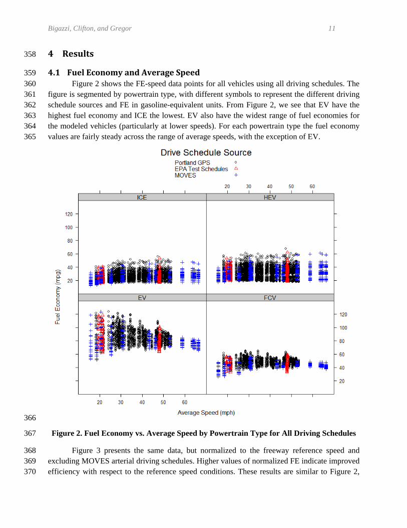
4.1 FuelEconomyandAverageSpeed359 Figure 2 shows the FE-speed data points for all vehicles using all driving schedules. The 360

figure is segmented by powertrain type, with different symbols to represent the different driving 361 schedule sources and FE in gasoline-equivalent units. From Figure 2, we see that EV have the 362 highest fuel economy and ICE the lowest. EV also have the widest range of fuel economies for 363 the modeled vehicles (particularly at lower speeds). For each powertrain type the fuel economy 364 values are fairly steady across the range of average speeds, with the exception of EV. 365

366

Figure 2. Fuel Economy vs. Average Speed by Powertrain Type for All Driving Schedules 367

Figure 3 presents the same data, but normalized to the freeway reference speed and 368 excluding MOVES arterial driving schedules. Higher values of normalized FE indicate improved 369 efficiency with respect to the reference speed conditions. These results are similar to Figure 2, 370


but with some of the inter-vehicle overall fuel economy differences removed – thus illuminating 371 the impacts of average speed. ICE vehicle FE is generally flat from free-flow speed down to 372 around 35 mph, at which point FE begins to decrease. For HEV the FE is nearly flat for all 373 except the lowest-speed MOVES driving schedule. EV fuel economy increases with decreasing 374 speed from free-flow conditions, down to around 20-30 mph. FCV fuel economy also increases 375 somewhat as speed decreases. 376

377

Figure 3. Fuel Economy (Normalized to Reference Speed) vs. Average Speed by Powertrain 378 Type for Freeways 379

4.2 Fuel‐SpeedCurves380 This section presents the fitted FSC from Equation 4. Two example fits for freeway FSC 381

are shown in Figure 4. Here, two fitted FSC are shown along with the base data (using the 382 MOVES and OR-217 driving schedules). The example low-congestion-efficiency ICE vehicle is 383 a heavy, high-powered gasoline-fueled passenger car. The fit has an approximate R-squared 384 value of 0.96 (calculated as Nagelkerke’s generalized R-squared). The example high-congestion-385


efficiency ICE vehicle is a diesel-fueled passenger truck with moderate power and weight. This 386 fit has a generalized R-squared value of 0.86. 387

388

Figure 4. Example Freeway FSC Fits 389

Figure 5 shows fitted freeway FSC for all modeled vehicles, segmented by powertrain 390 type (again in gasoline-equivalent mpg). There is a wide variety of FE values and FSC shapes, as 391 expected from Figure 2 (note the different vertical scales). Generally, ICE vehicles have varying 392 relationships with speed (positive or negative) for speeds above 30 mph, and decreasing FE at 393 lower speeds below 30 mph. HEV are less sensitive to congestion, with some vehicles’ FE not 394 decreasing until below 20 mph. Some HEV have about the same FE performance as ICE vehicles 395 – particularly those with low hybrid thresholds. EV and FCV both show increasing FE with 396 decreasing speed in Figure 5, down to a speed in the range of 20-40 mph. 397

10 20 30 40 50 60 70

0

10

20

30

40

AvgSpd

Mp

g

Low Congestion Efficiency ICEHigh Congestion Efficiency ICE


398

Figure 5. Modeled Individual Freeway FSC by Powertrain Type 399

4.3 SensitivityofFuelEconomyinCongestiontoVehicleCharacteristics400 Fuel economy can vary widely among vehicles for any one driving schedule, as 401

illustrated in Figure 2. This is due to variability in both fuel rates and VSP distributions of 402 operating time. In this section we examine how vehicle characteristics influence the Fuel-Speed 403 data points. Of particular interest is which vehicle characteristics impact the shape of the FSC – 404 i.e., which characteristics most affect relative vehicle performance in congestion. This is 405 different from which vehicle characteristics impact overall fuel economy, and sometimes shows 406 opposite effects. For example, vehicle parameters that mostly improve FE at higher speeds 407 (decreased drag coefficients, for example) will result in poorer relative FE in congestion. 408

Sensitivity analyses show that vehicle weight, engine displacement/fuel cell power, RLC, 409 hybrid threshold, and accessory load are the vehicle characteristics that have the most impact on 410 the fuel economy effects of congestion. Higher vehicle weight, engine size, and accessory load 411 all decrease relative performance in congestion for ICE vehicles, while higher RLC increase 412 relative performance. Compared to cars, passenger trucks and SUV’s tend to have more weight 413 and engine power (which both reduce performance in congestion), but also higher RLC (which 414

10 20 30 40 50 60 70

0

10

20

30

40

50

LD ICE, Freeway

Average Speed (mph)

MP

G

10 20 30 40 50 60 70

0

20

40

60

80

100

120

LD EV, Freeway

Average Speed (mph)

MP

G

10 20 30 40 50 60 70

0

20

40

60

80

LD HEV, Freeway

Average Speed (mph)

MP

G

10 20 30 40 50 60 70

0

20

40

60

80

LD FCV, Freeway

Average Speed (mph)

MP

G


improves relative performance in congestion by disproportionately decreasing efficiency at high 415 speeds). Higher motor peak power slightly increases relative congestion performance for EV, but 416 higher fuel cell power rating decreases relative congestion performance for FCV. 417

HEV performance in congestion increases with hybrid threshold (since more low-power 418 driving is powered by recovered energy). For HEV the motor and battery characteristics 419 combined with the driving patterns will determine the true hybrid threshold. Assuming HEV 420 improve over time to allow higher hybrid thresholds, the relative HEV performance in 421 congestion will improve as well. Unlike ICE vehicles, HEV can improve their relative FE in 422 congestion with larger engine sizes, because they can utilize the larger ICE nearer optimum 423 efficiency for high power loads but turn off the combustion engine during low-power driving 424 events in congestion. In this study, motor peak power was not a limiting factor in relative 425 efficiency for HEV. High accessory power loads notably degrade the relative efficiency in 426 congestion for fuel efficient vehicles, since a greater portion of total energy demand in 427 congestion is from the static accessory load. Since much of the expected accessory load is from 428 air conditioning usage, improvements over time such as advanced window glazings and cabin 429 ventilation [28] can increase the relative FE in congestion for advanced vehicles. 430

Power demands vary due to external vehicle forces only (mass and RLC inputs), while 431 fuel rates are influenced by all vehicle attributes. From Equation 1, the RLC and vehicle mass 432 have larger impacts at higher speeds (the impact of RLC “C” increases with the cube of speed). 433 The impact of acceleration, however, is independent of mass or RLC. Thus, the VSP distribution 434 of high-speed freeway driving schedules (with higher speeds and fewer accelerations) is more 435 impacted by vehicle characteristics (mass and RLC) than the VSP distribution of arterial driving 436 schedules (with more accelerations and lower speeds). More generally, the VSP distribution of 437 vehicle activity in uncongested driving conditions is more impacted by vehicle characteristics 438 than in congested driving conditions. The same holds for arterial versus freeway driving, with 439 freeway driving more impacted by vehicle characteristics. 440

As demonstrated in Figure 5, there is a range of potential FSC shapes for each vehicle 441 type, depending on the specific vehicle characteristics. Projecting this array of characteristics for 442 future vehicle fleets in scenario analysis is impractical. The next section describes a suggested 443 approach for incorporating these FSC into scenario analysis. 444

5 ApplyingFuel‐SpeedCurvesforScenarioAnalysis445

This section describes a recommended method for applying advanced-vehicle FSC for 446 scenario analysis, considering the range of plausible curve shapes shown in Section 4. The 447 recommended approach is to use minimum/maximum sensitivity normalized FSC as the bounds 448 of congestion effects. Interpolating between these extreme curves provides speed-based FE 449 adjustment factors to calculate congestion effects on overall fuel economy. 450

The interpolation distance between the bound FSC is based on a new model input, 451 “Congestion Efficiency”, which describes the projected performance of each vehicle type in 452 congestion, with respect to “extreme case” vehicles. Congestion Efficiency ranges from 0 for 453


poorest performance to 1 for maximum relative efficiency performance. Using Congestion 454 Efficiency and upper and lower bound normalized FSC with curve fit parameters , and 455

, , respectively, the interpolated normalized FSC curve is calculated 456

457

∙ exp ∑ , 1 exp ∑ , . (6) 458

459 The determination of in scenario analysis is based on the sensitivities described in Section 460 4.3. This approach avoids introducing numerous new vehicle parameters to the scenario analysis, 461 while still allowing some assumptions about the future vehicle fleet to inform the congestion 462 adjustment values. 463

We selected extreme-case vehicles for FSC bounds based on comparison of the FSC 464 shapes and vehicle attributes. Those vehicles selected are the modeled vehicles of each vehicle 465 type with the highest and lowest relative FE in heavy congestion as compared to FE at free-flow 466 speed (for each facility type). The vehicle characteristics and FSC fit parameters for the selected 467 vehicles are shown in Table 1. The corresponding upper-bound and lower-bound FSC are shown 468 in Figure 6. The selected bounding vehicles in Table 1 are not the most extreme combinations of 469 attributes possible. Rather, they are modeled mixes of vehicle attributes considered possible (if 470 not probable) based on the literature. 471


Table1.Extreme‐CaseVehicles:CharacteristicsandFSCFitParameters472 Freeways

ICE* HEV* EV** FCV** Congestion Efficiency Low High Low High Low High Low High

Passenger Car/Truck Car Truck Car Car Car Car Car Car Curb Weight (lbs) 5,000 2,500 2,504 2,000 3,800 2,000 3,000 2,000 Engine Displ. (L) 4.5 2.0 1.1 2.0 NA NA NA NA RLC: A 156.46 235.01 156.46 156.46 156.46 156.46 156.46 156.46 RLC: B 2.002 3.039 2.002 2.002 2.002 2.002 2.002 2.002 RLC: C 0.493 0.748 0.493 0.493 0.493 0.493 0.493 0.493 Motor Peak Power/

Fuel Cell Rating (kW) NA NA 68 10 80 100 140 40

Hybrid Threshold (kW) NA NA 2 4 NA NA NA NA Accessory Power (kW) 0.75 0.75 4 0.75 4 0.75 4 0.75 Total Peak Power (kW) 220 98 123 108 80 100 140 40

Specific Power (W/kg) 97 86 108 119 46 110 103 44 α0 1.514 2.331 1.892 3.122 2.911 4.236 1.984 3.048 α1 0.1112 0.0809 0.1321 0.0667 0.1132 0.0511 0.1324 0.0955 α2 -0.0029 -0.0025 -0.0041 -0.0025 -0.0034 -0.0019 -0.0037 -0.0032 α3 3.63E-5 2.94E-5 5.78E-5 3.44E-5 4.55E-5 2.41E-5 4.60E-5 4.27E-5 α4 -1.73E-7 -1.15E-7 -2.90E-7 -1.63E-7 -2.27E-7 -1.04E-7 -2.18E-7 -2.00E-7

Arterial ICE* HEV* EV** FCV**

Congestion Efficiency Low High Low High Low High Low High

Passenger Car/Truck Car Truck Car Car Car Car Car Car Curb Weight (lbs) 3,750 2,500 3,000 3,020 3,800 2,000 3,000 2,000 Engine Displ. (L) 4.5 2.0 1.8 1.3 NA NA NA NA RLC: A 156.46 235.01 156.46 154.69 156.46 156.46 156.46 156.46 RLC: B 2.002 3.039 2.002 1.977 2.002 2.002 2.002 2.002 RLC: C 0.493 0.748 0.493 0.487 0.493 0.493 0.493 0.493 Motor Peak Power/

Fuel Cell Rating (kW) NA NA 60 10 80 100 140 40

Hybrid Threshold (kW) NA NA 2 2 NA NA NA NA Accessory Power (kW) 4 0.75 4 0.75 4 0.75 4 0.75 Total Peak Power (kW) 220 98 148 76 80 100 140 40

Specific Power (W/kg) 129 86 109 55 46 110 103 44 α0 1.392 2.331 1.803 2.71 2.911 4.236 1.984 3.048 α1 0.1145 0.0809 0.1204 0.0765 0.1132 0.0511 0.1324 0.0955 α2 -0.0029 -0.0025 -0.0034 -0.0031 -0.0034 -0.0019 -0.0037 -0.0032 α3 3.45E-5 2.94E-5 4.36E-5 4.77E-5 4.55E-5 2.41E-5 4.60E-5 4.27E-5 α4 -1.55E-7 -1.15E-7 -2.06E-7 -2.42E-7 -2.27E-7 -1.04E-7 -2.18E-7 -2.00E-7

* Gasoline-fueled, automatic transmission, engine indicated efficiency of 0.4, model year 2010 ** EV and FCV are the same vehicles for arterials and freeways, model year 2010


473

474

Figure 6. Upper and Lower Bound Normalized FSC 475

20 30 40 50 60

0.6

0.8

1.0

1.2

1.4

LD ICE Freeway

Speed

Mpg

Fac

tor

High Congestion Eff iciencyLow Congestion Eff iciency

20 30 40 50 60

0.6

0.8

1.0

1.2

1.4

LD HEV Freeway

Speed

Mpg

Fac

tor


20 30 40 50 60

0.6

0.8

1.0

1.2

1.4

LD EV Freeway

Speed

Mpg

Fac

tor


20 30 40 50 60

0.6

0.8

1.0

1.2

1.4

LD FCV Freeway

Speed

Mpg

Fac

tor


10 15 20 25 30 35

0.6

0.8

1.0

1.2

1.4

LD ICE Arterial

Speed

Mpg

Fac

tor


10 15 20 25 30 35

0.6

0.8

1.0

1.2

1.4

LD HEV Arterial

Speed

Mpg

Fac

tor

High Congestion EfficiencyLow Congestion Efficiency

10 15 20 25 30 35

0.6

0.8

1.0

1.2

1.4

LD EV Arterial

Speed

Mpg

Fac

tor


10 15 20 25 30 35

0.6

0.8

1.0

1.2

1.4

LD FCV Arterial

Speed

Mpg

Fac

tor

High Congestion EfficiencyLow Congestion Efficiency


Table 2 lists the vehicle characteristics that are expected to impact the relative efficiency 476 in congestion ( ) for each vehicle powertrain type. This table is based on sensitivity analysis of 477 the modeled vehicle attributes and FSC. Qualitative projection of these attributes can be used to 478 set the new model input, Congestion Efficiency, between 0 and 1. The median Congestion 479 Efficiency value is 0.5, which puts the FE adjustment curve midway between the extreme curves 480 shown in Figure 6. If we expect, for example, average HEV to get lighter over time, we can set 481 the Congestion Efficiency to trend upward for future model years. Note again that is 482 increased both by attributes that improve FE in congestion and by attributes that 483 disproportionately decrease FE at higher speeds. 484

Table2.VehicleCharacterisitcsInfluencingRelativeCongestionEfficiency485 Powertrain type Low Relative Congestion Efficiency High Relative Congestion Efficiency

ICE heavier weight, larger engine, lower RLC, gasoline fuel, higher accessory loads,

earlier model year

lighter weight, smaller engine, higher RLC, diesel fuel, lower accessory loads,

later model year

HEV heavier weight, smaller ICE, lower RLC, lower hybrid threshold, gasoline fuel,

higher accessory loads, earlier model year

lighter weight, larger ICE, higher RLC, higher hybrid threshold, diesel fuel,

lower accessory loads, later model year

EV heavier weight, lower RLC, higher accessory loads

lighter weight, higher RLC, lower accessory loads

FCV heavier weight, higher fuel cell power rating, lower RLC, higher accessory loads

lighter weight, lower fuel cell power rating, higher RLC, lower accessory loads

486 As a final consideration, we examine the potential impacts of these FSC on overall FE. 487

Using a Congestion Efficiency of 0.5, at 25 mph the freeway ICE FE adjustment factor is 0.94 488 and all three advanced powertrain vehicle types have FE adjustments over 1 (i.e. efficiency 489 benefits). On arterials, the minimum adjustment factor at 20 mph (for ICE) is 0.92. Thus, the 490 potential adjustments to FE for typical congestion are small. With evolving vehicle fleets 491 containing more advanced vehicles, it is unlikely that the net effect of congestion on FE will be 492 substantially detrimental – and the net effect could be beneficial. 493

6 Conclusions494

This paper describes research undertaken to establish plausible fuel-speed curves (FSC) 495 for advanced vehicles, to be used in long-term transportation scenario analysis. We use the PERE 496 fuel consumption model with real-world driving schedules and a range of advanced vehicle 497 characteristics to estimate vehicle fuel economy in varying traffic conditions. The fuel-speed 498 data points are then used to generate normalized fuel economy versus average speed curves for 499 each of 145 modeled vehicles. 500

Analysis of the FSC shows that advanced powertrain vehicles are expected to perform 501 better in congestion than ICE vehicles (with respect to FE at free-flow speeds). Many ICE 502 vehicles do not lose fuel efficiency until traffic slows to about 30 mph. HEV are less sensitive to 503


average speed changes than ICE vehicles, and tend to maintain their fuel efficiency down to 20 504 mph, due to recaptured braking energy. Fuel efficiency increases for EV down to about 20-30 505 mph, below which it degrades. FCV have similar FE effects to EV, though with less sensitivity 506 to speed. 507

Besides powertrain type, congestion effects vary with other vehicle characteristics as 508 well. Relative fuel efficiency at lower speeds improves for vehicles with lighter weight, smaller 509 engines, higher hybrid thresholds, and lower accessory loads (such as air conditioning). Relative 510 performance in congestion can also improve with attributes that disproportionately decrease FE 511 at higher speeds, such as higher aerodynamic drag and rolling resistance factors. 512

Considering the normalized FSC sensitivity to multiple attributes, we propose a bounded 513 approach for applying the modeled FSC in scenario analysis. In the proposed method, FE 514 adjustments are an interpolation between extreme-case FSC, based on projection of relative 515 congestion efficiency. This allows adjustment for vehicle trends over time without requiring 516 specificity in the vehicle fleet characteristics. 517

In conclusion, the modeled FSC show that advanced powertrain vehicles can reduce or 518 reverse the fuel efficiency losses associated with typical roadway congestion. On the other hand, 519 advanced vehicles with certain characteristics (heavy and with high accessory power loads, for 520 example) can still have poor relative performance in congestion. The results of this research can 521 assist with broader analysis of the role these differences will play in total fuel consumption and 522 emissions from roadway travel. 523

References524

[1] D. Schrank, T. Lomax, and B. Eisele, “Urban Mobility Report 2011,” Texas Transportation 525 Institute, College Station, TX, Sep. 2011. 526

[2] S. E. Plotkin and M. K. Singh, “Multi-Path Transportation Futures Study: Vehicle 527 Characterization and Scenario Analyses,” Argonne National Laboratory (ANL), 2009. 528

[3] B. Gregor, “Greenhouse Gas Statewide Transportation Emissions Planning Model 529 (GreenSTEP Model) Documentation - Draft.” Oregon Department of Transportation, Nov-530 2010. 531

[4] E. Nam and R. Giannelli, “Fuel Consumption Modeling of Conventional and Advanced 532 Technology Vehicles in the Physical Emission Rate Estimator (PERE),” U.S. 533 Environmental Protection Agency, Draft EPA420-P-05-001, Feb. 2005. 534

[5] M. Barth and K. Boriboonsomsin, “Real-World Carbon Dioxide Impacts of Traffic 535 Congestion,” Transportation Research Record: Journal of the Transportation Research 536 Board, vol. 2058, pp. 163–171, 2008. 537

[6] M. Barth, G. Scora, and T. Younglove, “Estimating emissions and fuel consumption for 538 different levels of freeway congestion,” Transportation Research Record: Journal of the 539 Transportation Research Board, vol. 1664, pp. 47–57, 1999. 540

[7] A. Bigazzi and M. Figliozzi, “An Analysis of the Relative Efficiency of Freeway 541 Congestion Mitigation as an Emissions Reduction Strategy,” in 90th Annual Meeting of the 542 Transportation Research Board, Washington, D.C., 2011. 543


[8] T. Barlow and P. Boulter, “Emissions factors 2009: Report 2 - a review of the average-544 speed approach for estimating hot exhaust emissions,” UK Department for Transport, 545 Research report PPR355, Jun. 2009. 546

[9] R. Smit, A. L. Brown, and Y. C. Chan, “Do air pollution emissions and fuel consumption 547 models for roadways include the effects of congestion in the roadway traffic flow?,” 548 Environmental Modelling and Software, vol. 23, no. 10-11, pp. 1262–1270, 2008. 549

[10] U.S. Environmental Protection Agency, “Motor Vehicle Emission Simulator (MOVES) 550 2010 User’s Guide,” Washington, D.C., EPA-420-B-09-041, Dec. 2009. 551

[11] U.S. Environmental Protection Agency, “Final Technical Support Document: Fuel 552 Economy Labeling of Motor Vehicle Revisions to Improve Calculation of Fuel Economy 553 Estimates,” Washington, D.C., EPA420-R-06-017, Dec. 2006. 554

[12] S. C. Davis, S. W. Diegel, and R. G. Boundy, “Transportation Energy Data Book: Edition 555 29,” Oak Rige National Laboratory, Oak Ridge, TN, ORNL-6985, Jul. 2010. 556

[13] T. Markel et al., “ADVISOR: a systems analysis tool for advanced vehicle modeling,” 557 Journal of Power Sources, vol. 110, no. 2, pp. 255-266, Aug. 2002. 558

[14] M. Singh, A. Vyas, and E. Steiner, “VISION Model: Description of Model Used to 559 Estimate the Impact of Highway Vehicle Technologies and Fuels on Energy Use and 560 Carbon Emissions to 2050,” Argonne National Laboratory, ANL/ESD/04-1, Dec. 2003. 561

[15] M. Earleywine, J. Gonder, T. Markel, and M. Thornton, “Simulated fuel economy and 562 performance of advanced hybrid electric and plug-in hybrid electric vehicles using in-use 563 travel profiles,” in Vehicle Power and Propulsion Conference (VPPC), 2010 IEEE, 2010, 564 pp. 1-6. 565

[16] C. Samaras and K. Meisterling, “Life Cycle Assessment of Greenhouse Gas Emissions 566 from Plug-in Hybrid Vehicles: Implications for Policy,” Environmental Science & 567 Technology, vol. 42, no. 9, pp. 3170-3176, May 2008. 568

[17] C. Silva, M. Ross, and T. Farias, “Evaluation of energy consumption, emissions and cost of 569 plug-in hybrid vehicles,” Energy Conversion and Management, vol. 50, no. 7, pp. 1635-570 1643, Jul. 2009. 571

[18] A. Delorme, D. Karbowski, and P. Sharer, “Evaluation of fuel consumption potential of 572 medium and heavy duty vehicles through modeling and simulation.,” Argonne National 573 Laboratory (ANL), 2010. 574

[19] G. Fontaras, P. Pistikopoulos, and Z. Samaras, “Experimental evaluation of hybrid vehicle 575 fuel economy and pollutant emissions over real-world simulation driving cycles,” 576 Atmospheric Environment, vol. 42, no. 18, pp. 4023-4035, Jun. 2008. 577

[20] A. Alessandrini and F. Orecchini, “A driving cycle for electrically-driven vehicles in 578 Rome,” Proceedings of the Institution of Mechanical Engineers, Part D: Journal of 579 Automobile Engineering, vol. 217, no. 9, pp. 781-789, Jan. 2003. 580

[21] M. Barth et al., “Development of a Modal-Emissions Model,” Transportation Research 581 Board, Project 25-11, Apr. 2000. 582

[22] H. C. Frey, A. Unal, J. Chen, S. Li, and C. Xuan, “Methodology for Developing Modal 583 Emission Rates for EPA’s Multi-Scale Motor Vehicle & Equipment Emission System,” 584 U.S. Environmental Protection Agency, Ann Arbor, Michigan, EPA420-R-02-027, Aug. 585 2002. 586

[23] G. Song and L. Yu, “Estimation of Fuel Efficiency of Road Traffic by Characterization of 587 Vehicle-Specific Power and Speed Based on Floating Car Data,” Transportation Research 588


Record: Journal of the Transportation Research Board, vol. 2139, no. 1, pp. 11-20, Dec. 589 2009. 590

[24] E. Nam, “Proof of Concept Investigation for the Physical Emission Rate Estimator(PERE) 591 for MOVES,” U.S. Environmental Protection Agency, Ann Arbor, Michigan, EPA420-R-592 03-005, Feb. 2003. 593

[25] J. Koupal, L. Landman, E. Nam, J. Warila, E. Glover, and R. Giannelli, “MOVES2004 594 Energy and Emissions Inputs,” U.S. Environmental Protection Agency, Washington, D.C., 595 EPA420-P-05-003, Mar. 2005. 596

[26] Oregon Department of Transportation, “Traffic Volumes and Vehicle Classification,” 24-597 Aug-2010. [Online]. Available: 598 http://highway.odot.state.or.us/cf/highwayreports/traffic_parms.cfm. [Accessed: 03-Nov-599 2010]. 600

[27] U.S. Environmental Protection Agency, “MOVES2010 Highway Vehicle Population and 601 Activity Data,” Washington, D.C., EPA-420-R-10-026, Nov. 2010. 602

[28] R. Farrington and J. Rugh, “Impact of vehicle air-conditioning on fuel economy, tailpipe 603 emissions, and electric vehicle range,” in Earth Technologies Forum, WDC, 2000. 604

[29] S. Sugawara and D. Niemeier, “How much can vehicle emissions be reduced? Exploratory 605 analysis of an upper boundary using an emissions-optimized trip assignment,” 606 Transportation Research Record, vol. 1815, pp. 29-37, 2002. 607

608

modeling the effects of congestion on fuel economy for

Documents