modeling the radar return of powerlines using an
TRANSCRIPT

Rochester Institute of Technology Rochester Institute of Technology
RIT Scholar Works RIT Scholar Works
Theses
7-26-2016
Modeling the Radar Return of Powerlines Using an Incremental Modeling the Radar Return of Powerlines Using an Incremental
Length Diffraction Coefficient Approach Length Diffraction Coefficient Approach
Douglas Macdonald [email protected]
Follow this and additional works at: https://scholarworks.rit.edu/theses
Recommended Citation Recommended Citation Macdonald, Douglas, "Modeling the Radar Return of Powerlines Using an Incremental Length Diffraction Coefficient Approach" (2016). Thesis. Rochester Institute of Technology. Accessed from
This Dissertation is brought to you for free and open access by RIT Scholar Works. It has been accepted for inclusion in Theses by an authorized administrator of RIT Scholar Works. For more information, please contact [email protected].

Modeling the Radar Return of Powerlines Using an Incremental
Length Diffraction Coefficient Approach
by
Douglas Macdonald
B.S. Virginia Military Institute, 2005
M.S. Air Force Institute of Technology, 2010
A dissertation submitted in partial fulfillment of the
requirements for the degree of Doctor of Philosophy
in the Chester F. Carlson Center for Imaging Science
College of Science
Rochester Institute of Technology
July 26, 2016
Signature of the Author
Accepted byCoordinator, Ph.D. Degree Program Date
CHESTER F. CARLSON CENTER FOR IMAGING SCIENCE
COLLEGE OF SCIENCE
ROCHESTER INSTITUTE OF TECHNOLOGY
ROCHESTER, NEW YORK
CERTIFICATE OF APPROVAL
Ph.D. DEGREE DISSERTATION
The Ph.D. Degree Dissertation of Douglas Macdonaldhas been examined and approved by the
dissertation committee as satisfactory for thedissertation required for the
Ph.D. degree in Imaging Science
Dr. Michael Gartley, Dissertation Advisor
Dr. Raluca Felea, External Chair
Dr. John Kerekes
Dr. David Messinger
Date
2

Modeling the Radar Return of Powerlines Using an Incremental
Length Diffraction Coefficient Approach
by
Douglas Macdonald
Submitted to theChester F. Carlson Center for Imaging Science
in partial fulfillment of the requirementsfor the Doctor of Philosophy Degree
at the Rochester Institute of Technology
Abstract
A method for modeling the signal from cables and powerlines in Synthetic Aperture Radar(SAR) imagery is presented. Powerline detection using radar is an active area of research.Accurately identifing the location of powerlines in a scene can be used to aid pilots of lowflying aircraft in collision avoidance, or map the electrical infrastructure of an area. Thefocus of this research was on the forward modeling problem of generating the powerlineSAR signal from first principles. Previous work on simulating SAR imagery involved meth-ods that ranged from efficient but insufficiently accurate, depending on the application, tomore exact but computationally complex. A brief survey of the numerous ways to modelthe scattering of electromagnetic radiation is provided. A popular tool that uses the geo-metric optics approximation for modeling imagery for remote sensing applications acrossa wide range of modalities is the Digitial Imaging and Remote Sensing Image Generation(DIRSIG) tool. This research shows the way in which DIRSIG generates the SAR phasehistory is unique compared to other methods used. In particular, DIRSIG uses the geo-metric optics approximation for the scattering of electromagnetic radiation and builds thephase history in the time domain on a pulse-by-pulse basis. This enables an efficient gener-ation of the phase history of complex scenes. The drawback to this method is the inabilityto account for diffraction. Since the characteristic diameter of many communication cablesand powerlines is on the order of the wavelength of the incident radiation, diffraction isthe dominant mechanism by which the radiation gets scattered for these targets. Com-parison of DIRSIG imagery to field data shows good scene-wide qualitative agreement aswell as Rayleigh distributed noise in the amplitude data, as expected for coherent imagingwith speckle. A closer inspection of the Radar Cross Sections of canonical targets such astrihedrals and dihedrals, however, shows DIRSIG consistently underestimated the scat-tered return, especially away from specular observation angles. This underestimation was
3

4
particularly pronounced for the dihedral targets which have a low acceptance angle in ele-vation, probably caused by the lack of a physical optics capability in DIRSIG. Powerlineswere not apparent in the simulated data.
For modeling powerlines outside of DIRSIG using a standalone approach, an Incremen-tal Length Diffraction Coefficient (ILDC) method was used. Traditionally, this methodis used to model the scattered radiation from the edge of a wedge, for example the edgeson the wings of a stealth aircraft. The Physical Theory of Diffraction provides the 2Ddiffraction coefficient and the ILDC method performs an integral along the edge to extendthis solution to three dimensions. This research takes the ILDC approach but instead ofusing the wedge diffraction coefficient, the exact far-field diffraction coefficient for scat-tering from a finite length cylinder is used. Wavenumber-diameter products are limitedto less than or about 10 (k · a . 10). For typical powerline diameters, this translates toX-band frequencies and lower. The advantage of this method is it allows exact 2D solu-tions to be extended to powerline geometries where sag is present and it is shown to bemore accurate than a pure physical optics approach for frequencies lower than millimeterwave. The Radar Cross Sections produced by this method were accurate to within theexperimental uncertainty of measured RF anechoic chamber data for both X and C-bandfrequencies across an 80 arc for 5 different target types and diameters. For the X-banddata, the mean error was 6.0% for data with 9.5% measurement uncertainty. For the C-band data, the mean error was 11.8% for data with 14.3% measurement uncertainty. Thebest results were obtained for X-band data in the HH polarization channel within a 20
arc about normal incidence. For this configuration, a mean error of 3.0% for data with ameasurement uncertainty of 5.2% was obtained. The least accurate results were obtainedfor X-band data in the VV polarization channel within a 20 arc about normal incidence.For this configuration, a mean error of 8.9% for data with a measurement uncertainty of5.9% was obtained. This error likely arose from making the smooth cylinder assumption,which neglects the semi-open waveguide TE contribution from the grooves in the helicallywound powerline. For field data in an actual X-band circular SAR collection, a meanerror of 3.3% for data with a measurement uncertainty of 3.3% was obtained in the HHchannel. For the VV channel, a mean error of 9.9% was obtained for data with a mea-surement uncertainty of 3.4%. Future work for improving this method would likely entailadding a far-field semi-open waveguide contribution to the 2D diffraction coefficient forTE polarized radiation. Accounting for second order diffractions between closely spacedpowerlines would also lead to improved accuracy for simulated field data.

Acknowledgements
I would first like to express my sincere appreciation to my research advisor, Dr. MichaelGartley. The effort he put in to helping me setup the DIRSIG simulation was instrumentalin this research. His support, words of encouragement, and knowledge of 90’s culturehelped to pull me through the many obstacles I encountered. I would also like to givemy gratitude to Dr. John Kerekes for filling in as a backup advisor. The feedback heprovided was crucial to ensuring this work was well communicated and relevant. Dr.David Messinger also provided valuable insight as a member of the committee. The timehe took away from his duties as Department Head for the Center for Imaging Science tobe a member of my committee was much appreciated. Finally I would also like to thankDr. Raluca Felea, my external committee member, for making the commitment to be apart of my research as well.
This research would not have been possible without the help from Dr. Kamal Sarabandiand Dr. Leland Pierce. The powerline RCS measurements were critical for validating thiswork.
To all my fellow classmates, thank you for making this a wonderful experience. Fromthe classroom to Graduate Laboratory and to MacGregor’s, you all helped to make mystudies less painful. To my Rochester friends, thank you for being a part of my time here,giving me the most memorable experiences, and helping to show me all this place had tooffer. To my office mates, it has been an honor working with you. You all have helped tokeep me motivated and in high spirits. I look forward to working alongside you all in ourfuture endeavors.
Finally to my family. For every step of my journey, they have been by my side withunconditional love and support. They mean the world to me.
5

Contents
1 Introduction 15
2 Background 182.1 GRECOSAR . . . . . . . . . . . . . . . . . . . . . . . . . . . . . . . . . . . 212.2 SARAS . . . . . . . . . . . . . . . . . . . . . . . . . . . . . . . . . . . . . . 222.3 POV-Ray . . . . . . . . . . . . . . . . . . . . . . . . . . . . . . . . . . . . . 252.4 DIRSIG . . . . . . . . . . . . . . . . . . . . . . . . . . . . . . . . . . . . . . 262.5 FDTD . . . . . . . . . . . . . . . . . . . . . . . . . . . . . . . . . . . . . . . 282.6 Millimeter-wave Physical Optics Model . . . . . . . . . . . . . . . . . . . . . 302.7 Xpatch . . . . . . . . . . . . . . . . . . . . . . . . . . . . . . . . . . . . . . . 322.8 Summary . . . . . . . . . . . . . . . . . . . . . . . . . . . . . . . . . . . . . 33
3 Theory 343.1 Radar Cross Section Definition . . . . . . . . . . . . . . . . . . . . . . . . . 353.2 Modeling Electromagnetic Propagation . . . . . . . . . . . . . . . . . . . . . 36
3.2.1 Maxwell’s Equations . . . . . . . . . . . . . . . . . . . . . . . . . . . 393.2.2 Geometric Optics . . . . . . . . . . . . . . . . . . . . . . . . . . . . . 413.2.3 Geometric Theory of Diffraction . . . . . . . . . . . . . . . . . . . . 433.2.4 Scalar Diffraction Theory . . . . . . . . . . . . . . . . . . . . . . . . 453.2.5 Physical Optics . . . . . . . . . . . . . . . . . . . . . . . . . . . . . . 493.2.6 Modified Equivalent Current Approximation . . . . . . . . . . . . . 523.2.7 Physical Theory of Diffraction . . . . . . . . . . . . . . . . . . . . . 56
3.3 Power Line Modeling Using ILDC’s . . . . . . . . . . . . . . . . . . . . . . . 573.3.1 Physical model . . . . . . . . . . . . . . . . . . . . . . . . . . . . . . 583.3.2 2D Diffraction Coefficient . . . . . . . . . . . . . . . . . . . . . . . . 603.3.3 Incremental Length Diffraction Coefficient (ILDC) . . . . . . . . . . 623.3.4 SAR Phase History Simulation . . . . . . . . . . . . . . . . . . . . . 62
3.4 Summary . . . . . . . . . . . . . . . . . . . . . . . . . . . . . . . . . . . . . 64
6

CONTENTS 7
4 Methods 664.1 Baseline DIRSIG Assessment . . . . . . . . . . . . . . . . . . . . . . . . . . 674.2 Power Line Modeling . . . . . . . . . . . . . . . . . . . . . . . . . . . . . . . 75
4.2.1 Anechoic Chamber Measurements . . . . . . . . . . . . . . . . . . . 754.2.2 Gotcha Power Line RCS Comparison . . . . . . . . . . . . . . . . . . 80
5 Results 845.1 DIRSIG Results . . . . . . . . . . . . . . . . . . . . . . . . . . . . . . . . . . 855.2 Power Line Modeling Results . . . . . . . . . . . . . . . . . . . . . . . . . . 90
5.2.1 Anechoic Chamber Data . . . . . . . . . . . . . . . . . . . . . . . . . 905.2.2 AFRL Gotcha Data . . . . . . . . . . . . . . . . . . . . . . . . . . . 105
5.3 Summary . . . . . . . . . . . . . . . . . . . . . . . . . . . . . . . . . . . . . 111
6 Conclusion and Future Work 113
Appendices 125
A ILDC Module 126
B RCS Simulation Code 136
C Phase History Simulation Code 140

List of Figures
2.1 Image of two buildings with different material properties generated usingSARAS. Higher order wall-ground reflections are apparent for both build-ings [1]. . . . . . . . . . . . . . . . . . . . . . . . . . . . . . . . . . . . . . . 24
2.2 (Left) actual and (Right) simulated images of the Wynn Hotel. Specialfeatures in each image are labeled with corresponding letters [2]. . . . . . . 25
2.3 Simulated amplitude of field reflected from both a smooth and rough plateusing FDTD [3]. . . . . . . . . . . . . . . . . . . . . . . . . . . . . . . . . . 29
2.4 Geometric powerline model used by Sarabandi, K. [4]. . . . . . . . . . . . . 302.5 Simulated versus experimental RCS’s at 94 GHz for 4 different powerlines
in the VV channel. Bragg scattering peaks were accurately modeled by aPO approach at millimeter wavelengths [4]. . . . . . . . . . . . . . . . . . . 32
3.1 Fermat’s Principle for Edge Diffraction. . . . . . . . . . . . . . . . . . . . . 443.2 Geometry for Scalar Diffraction (Kirchoff) Integral. . . . . . . . . . . . . . . 463.3 Plot of a catenary. . . . . . . . . . . . . . . . . . . . . . . . . . . . . . . . . 593.4 Plot showing the normalized 2D RCS of a circular cylinder for various radii
at normal incidence. The noisy signature at the end was caused by machineprecision errors which arose when too many terms were used for the calcula-tion. Physical optics would be the preferable method in this high-frequencyregime. The ‖‖ and ⊥⊥ subscripts refer to incident and outgoing TM andTE modes, respectively. . . . . . . . . . . . . . . . . . . . . . . . . . . . . . 61
3.5 Depiction of the orientations of the polarization basis vectors from the air-craft’s frame of reference (H and V polarizations) and the powerline’s frameof reference (TE and TM polarizations). The definitions shown above wereused to convert the polarization amplitudes from one frame to another. . . 63
8

LIST OF FIGURES 9
4.1 Process imagery for Gotcha collection. (a) Total power image of AFRL dataproduced employing RITSAR using all 360 of azimuth for backprojectionprocessing. Canonical targets appears as point sources in the top-left por-tion of the image. (b) Image of view for which powerlines were apparent inthe upper-right portion of image. . . . . . . . . . . . . . . . . . . . . . . . . 68
4.2 Locations of canonical targets in the scene provided by AFRL/SNA [5]. . . 694.3 Plot showing the calibration offsets calculated using each of the canonical
targets. Although the targets were of different sizes and types and placedat different orientations, the calculated offsets were very similar. The rangeof the plot matches the range of the intensity scale for the raw image. Themean value indicated by the blue bar represented the actual offset used. . . 71
4.4 Flight paths used to collect the AFRL data for all 8 passes. . . . . . . . . . 734.5 Screen shot of Blender scene used for DIRSIG simulation. . . . . . . . . . . 744.6 Depiction of the anechoic chamber setup from the Michigan experiment [6]. 764.7 Image showing calibration sphere placed on top of mount [6]. . . . . . . . . 774.8 Image showing powerline placed on top of mount [6]. . . . . . . . . . . . . . 784.9 Images depicting the geometric cross-section of each object for which RCS
measurement were made: (a) 1.27 cm cylinder (b) 167.8 MCM Copper (c)556.5 MCM Aluminum (d) 954 MCM Aluminum & Steel and (e) 1431 MCMAluminum & Steel. All cables were ≈ 1 ft in length [6]. . . . . . . . . . . . 79
4.10 Image chip of isolated transmission lines. . . . . . . . . . . . . . . . . . . . . 804.11 Picture taken of a representative telephone pole configuration. The actual
telephone pole only had three transmission lines on top, configured similarlyto what is shown in the picture, as well as a thick bundle of communicationcables halfway up. Images of the actual telephone poles could not be obtained. 81
4.12 Physical model images. (a) Sketch of powerline in CAD software (b) 3Dpowerline plot (c) Side view of the top transmission line. . . . . . . . . . . . 82
5.1 Qualitative Image Comparisons: (top) AFRL Gotcha, (bottom) simulated. . 855.2 Intensity histograms for grassy field showing noise characteristics of data.
A good fit using a Rayleigh distribution was obtained for both the simu-lated DIRSIG data and the Gotcha field data. This is consistent with thenoise distribution expected for coherent imaging modalities. (left) DIRSIGsimulated, (right) Gotcha. . . . . . . . . . . . . . . . . . . . . . . . . . . . . 86
5.3 RCS plots for trihedral targets: (a) TR1 (b) TR2 (c) TR3 and (d) TR4.The target labels TR1-TR4 correspond to those in figure 4.2. The DIRSIGderived RCS’s consistently underestimate the observed return, likely due tothe absence of a physical optics capability. . . . . . . . . . . . . . . . . . . . 88

LIST OF FIGURES 10
5.4 RCS plots for trihedral and dihedral targets: (a) TR5 (b) TR6 (c) DR2and (d) DR6. The target labels TR5-DR6 correspond to those in figure4.2.The DIRSIG derived RCS’s consistently underestimate the observed re-turn, likely due to the absence of a physical optics capability. This effectis especially pronounced for the dihedral targets which have small accep-tance angle in elevation. Also absent in the simulated dihedral RCS’s aresidelobes, which require physical optics to be modeled. . . . . . . . . . . . . 89
5.5 View of finite cylinder at different aspects, as measured from plane normalto axial direction: (a) 0 (b) 20 (c) 40 (d) 80. Note the increasing viewof the endcap and decreasing view of the cylindrical portion. . . . . . . . . 92
5.6 Modeled X-band power line RCS compared to anechoic chamber measure-ments for 1.27 cm diameter (ka = 2.5) smooth cylinder: (top-pair) usingPhysical Optics and Physical Theory of Diffraction exclusively (bottom-pair) using exact smooth cylinder 2-D diffraction coefficient for cylindricalportion and PO/PTD for endcaps (left-pair) HH channel (right-pair) VVchannel. Error bars on the measured data are scaled by ± 1 standard de-viation. For the simulated data, error bounds depict the O (k · a)−1 errorassociated with using a stationary phase technique to evaluate the contourintegral along the edge adjoining the endcap and cylinder. . . . . . . . . . . 93
5.7 Modeled X-band power line RCS compared to anechoic chamber measure-ments for 167.8 MCM (ka = 2.4) copper power line: (top-pair) using Physi-cal Optics and Physical Theory of Diffraction exclusively (bottom-pair) us-ing exact smooth cylinder 2-D diffraction coefficient for cylindrical portionand PO/PTD for endcaps (left-pair) HH channel (right-pair) VV channel.Error bars on the measured data are scaled by ± 1 standard deviation.For the simulated data, error bounds depict the O (k · a)−1 error associatedwith using a stationary phase technique to evaluate the contour integralalong the edge adjoining the endcap and cylinder. . . . . . . . . . . . . . . . 94
5.8 Modeled X-band power line RCS compared to anechoic chamber measure-ments for 556.5 MCM (ka = 4.4) aluminum power line: (top-pair) usingPhysical Optics and Physical Theory of Diffraction exclusively (bottom-pair) using exact smooth cylinder 2-D diffraction coefficient for cylindricalportion and PO/PTD for endcaps (left-pair) HH channel (right-pair) VVchannel. Error bars on the measured data are scaled by ± 1 standard de-viation. For the simulated data, error bounds depict the O (k · a)−1 errorassociated with using a stationary phase technique to evaluate the contourintegral along the edge adjoining the endcap and cylinder. . . . . . . . . . . 95
LIST OF FIGURES 11
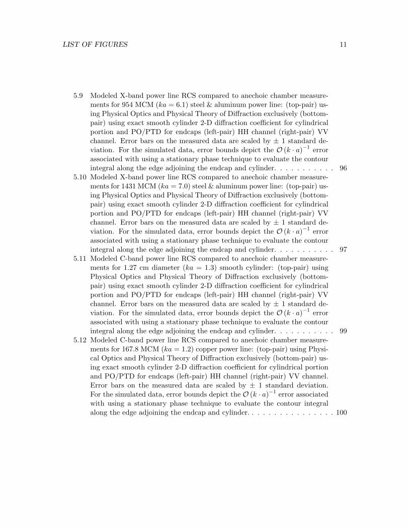
5.9 Modeled X-band power line RCS compared to anechoic chamber measure-ments for 954 MCM (ka = 6.1) steel & aluminum power line: (top-pair) us-ing Physical Optics and Physical Theory of Diffraction exclusively (bottom-pair) using exact smooth cylinder 2-D diffraction coefficient for cylindricalportion and PO/PTD for endcaps (left-pair) HH channel (right-pair) VVchannel. Error bars on the measured data are scaled by ± 1 standard de-viation. For the simulated data, error bounds depict the O (k · a)−1 errorassociated with using a stationary phase technique to evaluate the contourintegral along the edge adjoining the endcap and cylinder. . . . . . . . . . . 96
5.10 Modeled X-band power line RCS compared to anechoic chamber measure-ments for 1431 MCM (ka = 7.0) steel & aluminum power line: (top-pair) us-ing Physical Optics and Physical Theory of Diffraction exclusively (bottom-pair) using exact smooth cylinder 2-D diffraction coefficient for cylindricalportion and PO/PTD for endcaps (left-pair) HH channel (right-pair) VVchannel. Error bars on the measured data are scaled by ± 1 standard de-viation. For the simulated data, error bounds depict the O (k · a)−1 errorassociated with using a stationary phase technique to evaluate the contourintegral along the edge adjoining the endcap and cylinder. . . . . . . . . . . 97
5.11 Modeled C-band power line RCS compared to anechoic chamber measure-ments for 1.27 cm diameter (ka = 1.3) smooth cylinder: (top-pair) usingPhysical Optics and Physical Theory of Diffraction exclusively (bottom-pair) using exact smooth cylinder 2-D diffraction coefficient for cylindricalportion and PO/PTD for endcaps (left-pair) HH channel (right-pair) VVchannel. Error bars on the measured data are scaled by ± 1 standard de-viation. For the simulated data, error bounds depict the O (k · a)−1 errorassociated with using a stationary phase technique to evaluate the contourintegral along the edge adjoining the endcap and cylinder. . . . . . . . . . . 99
5.12 Modeled C-band power line RCS compared to anechoic chamber measure-ments for 167.8 MCM (ka = 1.2) copper power line: (top-pair) using Physi-cal Optics and Physical Theory of Diffraction exclusively (bottom-pair) us-ing exact smooth cylinder 2-D diffraction coefficient for cylindrical portionand PO/PTD for endcaps (left-pair) HH channel (right-pair) VV channel.Error bars on the measured data are scaled by ± 1 standard deviation.For the simulated data, error bounds depict the O (k · a)−1 error associatedwith using a stationary phase technique to evaluate the contour integralalong the edge adjoining the endcap and cylinder. . . . . . . . . . . . . . . . 100

LIST OF FIGURES 12
5.13 Modeled C-band power line RCS compared to anechoic chamber measure-ments for 556.5 MCM (ka = 2.2) aluminum power line: (top-pair) usingPhysical Optics and Physical Theory of Diffraction exclusively (bottom-pair) using exact smooth cylinder 2-D diffraction coefficient for cylindricalportion and PO/PTD for endcaps (left-pair) HH channel (right-pair) VVchannel. Error bars on the measured data are scaled by ± 1 standard de-viation. For the simulated data, error bounds depict the O (k · a)−1 errorassociated with using a stationary phase technique to evaluate the contourintegral along the edge adjoining the endcap and cylinder. . . . . . . . . . . 101
5.14 Modeled C-band power line RCS compared to anechoic chamber measure-ments for 954 MCM (ka = 3.0) steel & aluminum power line: (top-pair) us-ing Physical Optics and Physical Theory of Diffraction exclusively (bottom-pair) using exact smooth cylinder 2-D diffraction coefficient for cylindricalportion and PO/PTD for endcaps (left-pair) HH channel (right-pair) VVchannel. Error bars on the measured data are scaled by ± 1 standard de-viation. For the simulated data, error bounds depict the O (k · a)−1 errorassociated with using a stationary phase technique to evaluate the contourintegral along the edge adjoining the endcap and cylinder. . . . . . . . . . . 102
5.15 Modeled C-band power line RCS compared to anechoic chamber measure-ments for 1431 MCM (ka = 3.5) steel & aluminum power line: (top-pair) us-ing Physical Optics and Physical Theory of Diffraction exclusively (bottom-pair) using exact smooth cylinder 2-D diffraction coefficient for cylindricalportion and PO/PTD for endcaps (left-pair) HH channel (right-pair) VVchannel. Error bars on the measured data are scaled by ± 1 standard de-viation. For the simulated data, error bounds depict the O (k · a)−1 errorassociated with using a stationary phase technique to evaluate the contourintegral along the edge adjoining the endcap and cylinder. . . . . . . . . . . 103
5.16 Qualitative Image Comparisons: (left) AFRL Gotcha (right) simulated(top) platform at top-right (bottom) platform at bottom-left. . . . . . . . . 105
5.17 Quantitative RCS Comparisons: (left) HH channel (right) VV channel (top)platform at top-right (bottom) platform at bottom-left. . . . . . . . . . . . 107
5.18 Image chip of isolated transmission lines when the platform was at (a) top-right and (b) bottom-left of image. Four distinct signals are apparent inthe latter image even though only three transmission lines were observedon the telephone pole (plus the already accounted for single bundle of com-munication wires). This was observed for all 8 passes. . . . . . . . . . . . . 109
5.19 RCS Comparisons assuming no sag: (left) HH channel (right) VV channel(top) platform at top-right (bottom) platform at bottom-left. . . . . . . . . 110

List of Tables
4.1 AFRL platform parameters used for the DIRSIG simulation. . . . . . . . . 724.2 Material reflectivity parameters used for the DIRSIG simulation. . . . . . . 75
5.1 X-band results summary. . . . . . . . . . . . . . . . . . . . . . . . . . . . . 985.2 C-band results summary. . . . . . . . . . . . . . . . . . . . . . . . . . . . . 1045.3 AFRL Gotcha results summary. . . . . . . . . . . . . . . . . . . . . . . . . 108
13

List of Major Symbols
a Powerline diameter.
d 2D diffraction coefficient. For backscattering from an infinitely long, perfectly conduct-ing 1D object, This quantity is also equal to the Incremental Length DiffractionCoefficient.
D 3D diffraction coefficient.
Ei Incident field, oriented along the polarization direction.
Es Scattered field, oriented along the polarization direction.
k wavenumber.
k wavevector.
k · a wavenumber-diameter product.
Ψ Obliquity angle of incident/scattered radiation, measured from plane perpendicular tothe powerline’s axial direction.
β Obliquity angle of incident/scattered radiation, measured from the powerline’s axialdirection.
R Distance from receiver to target.
R Distance from receiver to target, oriented along propagation direction.
r Distance from a point on the powerline to a scene reference point.
σ Radar Cross Section.
14

Chapter 1
Introduction
Detecting powerlines is an important remote sensing application. The information gleanedfrom power line detection can be used to characterize an area’s power infrastructure. Itcan also be used in hazard avoidance applications for low flying aircraft. In both cases, apotential application can be found in humanitarian relief for natural disasters. Specifically,having the ability to remotely sense powerlines can give decision-makers a quick survey ofthe damage to a power grid over a wide area. It can also aid pilots of low flying search-and-rescue aircraft in mission planning. In the optical regime, powerlines do not oftenexhibit a strong return due to their smallness and the radiometry of the problem. Inthe radar regime, however, powerlines can be a very prominent feature in the processedimagery for certain viewing geometries. Since the diameter of a typical power line is oftenon the order of only a few wavelengths for radar, a significant portion of the return is dueto diffraction.
This research focused on modeling the radar return from power lines. There are nu-merous benefits that result from having an accurate model for powerline returns. Onebenefit is the ability to determine if a conceptual system will be able to perform pow-erline detection given the system’s operating parameters, such as carrier frequency andflight path. This benefit gives program managers the ability to predict if a given systemdesign can meet certain mission requirements with regards to powerline detection, avoid-ing significant hardware expense. Similarly, a second benefit would be to determine if anexisting system can perform the mission given its operating parameters. The enhancedcapability of a space-borne SAR system, for example, would illustrate this benefit. If themodel predicts powerline detection will be more effective on one pass than another, thisinformation can be used by mission planners to optimize the sensor’s tasking. Finally,a model of the powerline return for an existing system and operating parameters can beused to determine an a priori matched filter for post-processing on actual data. This is a
15

CHAPTER 1. INTRODUCTION 16
common application for forward modeled data.There has been much work recently on the development of software which simulates the
SAR signal for large urban scenes. An overview of the research in this area performed todate is provided in Chapter 2. In particular, an experimental capability has been addedto the Digital Imaging and Remote Sensing Image Generation (DIRISIG) tool for theradar imaging modality [7]. DIRSIG is a tool widely used in the Electro-optic/Infra-red(EO/IR) modalities which produces radiometrically accurate, physically based imagery[8]. DIRSIG is shown to simulate the SAR phase history for a given scene and operationalparameters and is unique to other software tools that have the same focus on modeling theSAR signal for complex scenes. There is also a plethora of tools available for modeling theRadar Cross Section of an object. One popular example is Xpatch [9], a tool used by theAir Force research labs which uses the Shooting and Bouncing of Rays (SBR) technique.Unfortunately, as will be explained later, SBR does not perform well for optically thinobjects such as powerlines at typical radar wavelengths. One effort made by Sarabandi, K.[4] resulted in a Method of Moments (MoM) approach for the specific purpose of modelingpowerline RCS’s. At millimeter-wave frequencies, evaluation of the source current integralwas simplified by making a physical optics approximation. However, this approximationbreaks down for wavenumber-diameter products . 1. All previous work considered, a gapis apparent for efficiently yet accurately modeling the radar return of powerlines in thisregime.
A brief overview of the methods used to model the scattering of Electromagnetic (EM)waves is provided in Chapter 3. This chapter begins by reviewing how a RCS is defined.The RCS of an object describes how efficiently it scatters radiation given its shape, materialproperties, the viewing angle, and the angle of incidence of the incoming radiation. Theremainder of Chapter 3 reviews the different ways to calculate how an object scattersEM radiation, with a concentration on how diffraction is modeled. As mentioned earlier,the dominant scattering mechanism by powerlines is due to diffraction. Diffraction is aphenomenon that describes how electromagnetic radiation scatters off obstructions. Thisphenomenon is most readily observed when the characteristic length of the scatteringobject is on the order of a few wavelengths. In the case of powerlines, typical diametersare on the order of a few to tens of centimeters. Since the wavelength of radiation in theradar regime is also typically on the order of a few centimeters, diffraction becomes thedominant scattering mechanism.
In order to provide an efficient, yet accurate, way of measuring powerlines, an Incre-mental Length Diffraction Coefficient (ILDC) approach was used in this research. TheILDC approach is traditionally used to model how edges scatter radiation in three di-mensions [10]. The approach has been adapted in this research for powerline modeling.The effort began with creating a physical model that accounted for both material and

CHAPTER 1. INTRODUCTION 17
geometric properties. The powerline was assumed to be a perfectly conducting smoothcylinder with sag described by a catenary. The two dimensional problem for scatteringinto the forward cone was then solved to yield a 2D diffraction coefficient. A 3D diffrac-tion coefficient was then derived using the ILDC approach developed by Mitzner. This 3Dcoefficient was then used to generate both powerline RCS’s that were later compared toexperimentally measured RCS’s. The 3D diffraction coefficient was also used to generatea SAR phase history. The scene resulting from this phase history was then compared toan actual circular SAR collection from the Air Force Research Labs (AFRL) [5].
The methods used to validate this ILDC approach are described in Chapter 4. First,a generic assessment of DIRSIG’s radar modality was performed. The scene used for theDIRSIG simulation roughly matched that of the AFRL field collection and included pow-erlines and canonical targets such as dihedrals and trihedrals. The parameters used for thesimulation closely matched what was provided in the AFRL auxiliary data. The assess-ment included not just an investigation of whether or not DIRSIG could model powerlines,but also how well it performed against the canonical targets. Additionally, DIRSIG’s abil-ity to simulate the noise present in a SAR image was assessed. Next, the ILDC approachfor generating 3D diffraction coefficients for powerlines was validated against data takenin an anechoic chamber by the University of Michigan [6]. Included in this discussionis a description of how the experiment was setup and calibrated. Finally, the simulatedpowerline phase history was compared to that observed in the field-measured AFRL data[5]. The method used to perform this comparison is also provided.
The results for each validation effort are provided in Chapter 5. For the DIRSIG assess-ment, good scene-wide qualitative agreement between the simulated and field extractedimagery was observed. The simulated imagery also exhibited Rayleigh distributed noise,as expected. Upon closer inspection, however, it was shown that DIRSIG was not capableof accurately modeling the RCS’s of the smaller canonical targets since it does not havea physical optics capability. Powerlines were also absent from the imagery due DIRSIG’suse of a geometric optics approximation which is inadequate for optically thin objects. Forthe experimentally measured RCS’s from the University of Michigan, overall agreementbetween the simulated and measured data was observed, with errors falling within the ex-perimental uncertainty. A few significant discrepancies were noted however, especially inthe VV channel. A discussion is provided on why the smooth cylinder approximation usedin this research would lead to errors in the VV channel. Similar results were obtained forthe AFRL data. Chapter 5 concludes with a discussion on sources of error and how theymay be mitigated in future work. Suggested follow-on efforts would include a correctionfor the 2D diffraction coefficient in the VV channel as well as additional field data withprecisely known ground truth that focuses on the powerline modeling problem.

Chapter 2
Background
The methods used to simulate SAR imagery are significantly different from those used tosimulate EO/IR imagery. For those most familiar with how a traditional optical systemworks, the most striking difference is the way in which an image is formed. In conventionaloptics, the spatial aperture collecting the signal is two dimensional. For SAR, the spatialaperture is the one-dimensional flight path of the platform. The temporal length of thereceived signal forms the second dimension. The time domain signal, before demodulation,is a measurement of the phase of the electric field. This is unlike conventional optics wherea detector element usually measures power, which is proportional to the time average ofthe electric field squared. Since SAR systems measure and record the phase of the electricfield, signal processing needs to be applied to form an interpretable image. This signalprocessing is usually done at the hardware level or in post-processing. This is in contrastto how an image is formed in optics, where the physics of light propagation does all ofthe signal processing. For example, in a single lens system, the phase of the electric fieldacross the aperture is mixed with the lens thickness function and is then matched filteredby the Fresnel convolution kernel. All of this signal processing is transparent to users oftraditional optical imaging systems.
The variability of signal processing methods that can be used to process SAR datapresents difficulties for methods attempting to simulate SAR imagery, using conventionalFourier optics. Measurements made by SAR systems are further up the imaging chainthan that of optical systems. For a SAR system, the measurement of the phase of theelectric field is made at the aperture level, whereas for traditional optics, measurementsare made after “Fresnel post-processing” and measuring the time average of the electricfield squared. As a result, the system transfer function of a SAR system is more complexand also much more customizable than that of a traditional optical system. Once anoptical system is built, the impulse response usually remains static. For SAR systems, the
18

CHAPTER 2. BACKGROUND 19
impulse response can change from one collection to another, based on a variety of factors.These include, but are not limited to, the length of the flight path, the characteristicsof the transmitted signal, and the different kinds of reconstruction algorithms that wereapplied to the recorded phase history. Additionally, since the reflectivity of a target canvary greatly across the length of the SAR aperture, applying a shift-invariant impulseresponse to a reflectivity map can lead to inaccurate results. For example, the impulseresponse of a perfect point reflector will be much different from the point spread function(PSF) for a point reflector which has a small acceptance angle. Along azimuth, the spatialfrequency region of support for the perfect reflector will be determined by the length of thefull synthetic aperture, whereas the target with the low acceptance angle will be smearedin azimuth, since only a fraction of the full aperture will have contained signal.
In addition to the differences in the image formation process, there are other moresubtle differences between conventional EO/IR and radar imaging modalities. Since SARinvolves coherent illumination of the target area, speckle is the dominant source of noise.Speckle is observed when the amplitude of the surface roughness is on the order, of orless than, a wavelength and the correlation length across the surface is much less than aresolution cell. When these conditions are met, the observed intensity of a single resolutioncell is determined by a sum of impulse responses with random phases [11].
Effects due to diffraction are also more pronounced in SAR since radar wavelengthsare longer than EO/IR wavelengths. Early SAR simulators modeled diffraction effects inSAR imagery in a statistical sense, similar to how speckle is modeled [3]. This workedfairly accurately at low resolution [3]. As the resolution of SAR systems has increasedin recent years, the need to use more accurate diffraction models has increased [3]. Thisis especially important in urban scenery where narrow streets can act as wave guides,rectangular structures can produce unattended diffractions, and strong scattering fromman-made surfaces that have edges or corners can dominate the return signal [3].
The methods for simulating SAR imagery or RCS’s presented in the following sec-tions each have their own specialty. As of yet, there is no general purpose radar simu-lator. One of the more widely used SAR simulators in the community is GRECOSAR[12, 13, 14, 15]. GRECOSAR uses high-frequency approximation techniques such asgeometric optics, physical optics, physical theory of diffraction, and incremental lengthdiffraction coefficients to generate the SAR signal. This is done on a pulse-by-pulse basis.GRECOSAR has been shown to produce radiometrically accurate results for naval ves-sels. Research on how well this tool models complex urban scenery is on-going but initialresults are promising [15]. Another well known SAR simulator is SARAS [16, 1]. This toolbuilds up the SAR signal in the frequency domain using a surface model that is discretizedinto rectangular facets. The scattering contribution from each facet is determined by thesurface properties of the material and the radiation diagram predicted by physical optics.

CHAPTER 2. BACKGROUND 20
Later versions of the tool could model multiple scattering by using geometric optics forall but the final bounce back to the receiver. Physical optics was then used to calculatethe scattered field on the final bounce.
GRECOSAR and SARAS are examples of code that have been specifically writtento simulate the SAR phase history for a given scene. Some examples of software toolstraditionally used for modeling in the optical regime that have been adapted for SARsimulation are POV-RAY [2] and DIRSIG [7, 8]. One of the effects commonly seen inurban imagery is displacement of a signal due to multiple bounce returns. This effectmanifests itself when a pulse bounces multiple times before finally coming back to thereceiver. Since the range of the pulse is determined by the time of flight, the signal isoften located farther downrange than the actual location of the last position the pulsewas scattered from. This can lead to reduced image interpretability. Ray-tracers suchas POV-RAY have been used to create efficiently images which replicate the effect ofmultiple bounces, but are otherwise radiometrically inaccurate. The intended use of thisprogram is to aid analysts in interpreting SAR imagery which contain large, complexstructures. Another tool adapted to simulating SAR imagery is DIRSIG. While DIRSIGis a mature and widely used tool for producing radiometrically accurate imagery in theEO/IR regime, its radar modality is still experimental at this stage. DIRSIG takes thegeometric optics approach to modeling the return signal and does not incorporate physicaloptics or any other high-frequency technique. The signal is built up on a pulse-by-pulsebasis by convolving the transmitted pulse with delta functions centered at the time of flightof each ray shot into the scene. The result is a tool which is efficient, models multiplescattering, and accounts for targets with dynamic, aspect-dependent reflectivities, but islimited by the geometric optics approximation.
For achieving a very high degree of accuracy, the computationally intensive FiniteDifference Time Delay (FDTD) [3] method has also been used. Due to the complexityof this approach and the stringent hardware requirements needed for implementation,simulations have been limited to simple objects commonly found in urban scenery. Whilethis method would be too complicated to use for modeling a complex scene given currenthardware capabilities, it has value in obtaining high fidelity results for simple, commonobjects.
Another accurate but computationally intense method found in the literature usesthe Method of Moments (MoM) [17]. More specifically, work done by Sarabandi, K. andMoonsoo, P. demonstrated how MoM could be used to model the source currents on thesurface of a powerline [4]. In the special case of millimeter-wave radiation, they simplifiedthe source current integral to a perturbation series that did not require the use of thecomputationally intensive MoM. The source currents in the millimeter-wave regime werecalculated using physical optics for the 0th-order term in the perturbation series. The
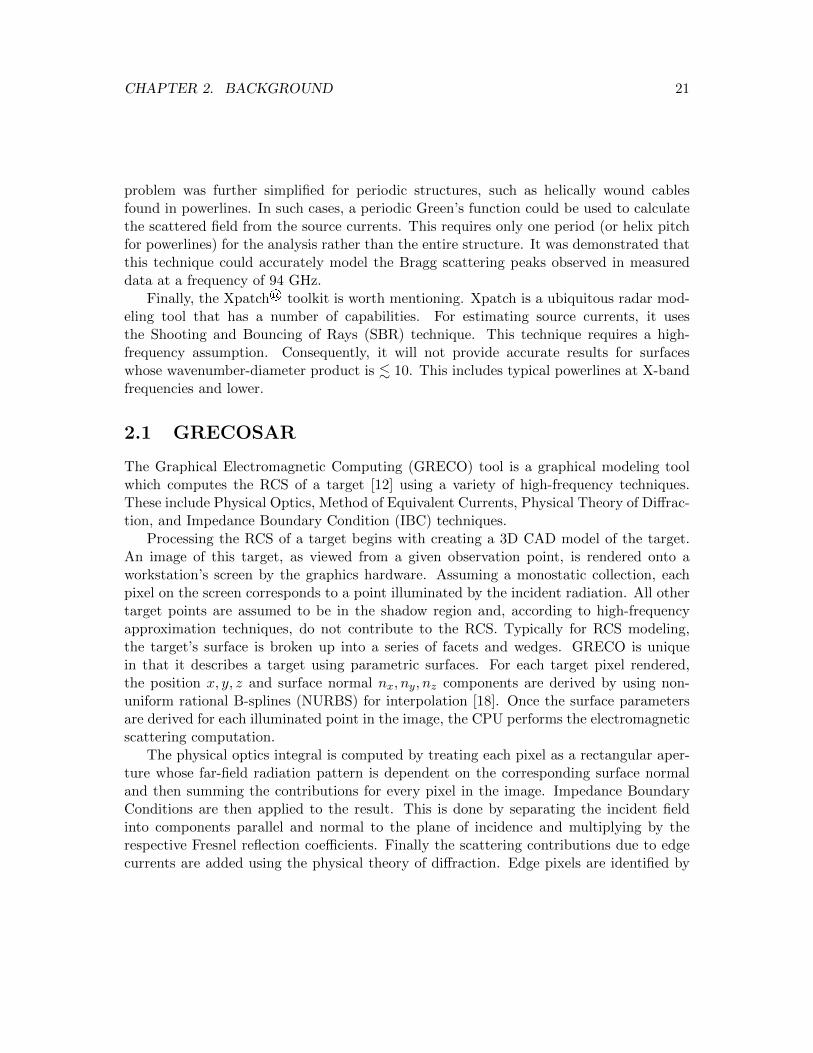
CHAPTER 2. BACKGROUND 21
problem was further simplified for periodic structures, such as helically wound cablesfound in powerlines. In such cases, a periodic Green’s function could be used to calculatethe scattered field from the source currents. This requires only one period (or helix pitchfor powerlines) for the analysis rather than the entire structure. It was demonstrated thatthis technique could accurately model the Bragg scattering peaks observed in measureddata at a frequency of 94 GHz.
Finally, the Xpatch® toolkit is worth mentioning. Xpatch is a ubiquitous radar mod-eling tool that has a number of capabilities. For estimating source currents, it usesthe Shooting and Bouncing of Rays (SBR) technique. This technique requires a high-frequency assumption. Consequently, it will not provide accurate results for surfaceswhose wavenumber-diameter product is . 10. This includes typical powerlines at X-bandfrequencies and lower.
2.1 GRECOSAR
The Graphical Electromagnetic Computing (GRECO) tool is a graphical modeling toolwhich computes the RCS of a target [12] using a variety of high-frequency techniques.These include Physical Optics, Method of Equivalent Currents, Physical Theory of Diffrac-tion, and Impedance Boundary Condition (IBC) techniques.
Processing the RCS of a target begins with creating a 3D CAD model of the target.An image of this target, as viewed from a given observation point, is rendered onto aworkstation’s screen by the graphics hardware. Assuming a monostatic collection, eachpixel on the screen corresponds to a point illuminated by the incident radiation. All othertarget points are assumed to be in the shadow region and, according to high-frequencyapproximation techniques, do not contribute to the RCS. Typically for RCS modeling,the target’s surface is broken up into a series of facets and wedges. GRECO is uniquein that it describes a target using parametric surfaces. For each target pixel rendered,the position x, y, z and surface normal nx, ny, nz components are derived by using non-uniform rational B-splines (NURBS) for interpolation [18]. Once the surface parametersare derived for each illuminated point in the image, the CPU performs the electromagneticscattering computation.
The physical optics integral is computed by treating each pixel as a rectangular aper-ture whose far-field radiation pattern is dependent on the corresponding surface normaland then summing the contributions for every pixel in the image. Impedance BoundaryConditions are then applied to the result. This is done by separating the incident fieldinto components parallel and normal to the plane of incidence and multiplying by therespective Fresnel reflection coefficients. Finally the scattering contributions due to edgecurrents are added using the physical theory of diffraction. Edge pixels are identified by

CHAPTER 2. BACKGROUND 22
discontinuities in the surface normal. For a given wedge angle, incidence angle, and po-larization, there is a corresponding diffraction coefficient. Diffraction coefficients act inmuch the same way as reflection coefficients as they relate the incident field amplitudeto the scattered field amplitude for a given geometry and polarization. A more detaileddiscussion of diffraction coefficients is provided in 3.2.7. The line integral along the edgesis then computed by summing the contributions from each edge pixel. Results shown in[12] demonstrated a high degree of accuracy when compared to numerical solutions. Usingonly physical optics, accurate RCS’s for non-stealth targets could be obtained.
GRECOSAR is a code that uses GRECO to compute the RCS of objects in a givenscene and simulates the SAR signal [13]. For each azimuth position, an image of thescene from the viewpoint of the platform is rendered. GRECO computes the frequencydependent RCS in the frequency domain. This response is applied to the time domainsignal by means of an inverse Fast Fourier Transform along the range dimension.
The GRECO code has been exhaustively validated for both canonical and complextargets [14]. GRECOSAR is relatively experimental but has been used in studies toevaluate SAR images of fisheries [13] and individual naval vessels [14]. In the literature[13, 14], much of the phenomenology observed in real world scenarios was captured bythe simulator [15]. Recently, GRECOSAR’s ability to model urban scenes has also beenevaluated. The study was mostly limited to an image of a box of gypsum on top ofa perfectly conducting plane. While examples of GRECOSAR’s ability to model morecomplex urban scenes has not been found in the literature, initial results for easily validatedsimple scenes were promising [15].
2.2 SARAS
The Synthetic Aperture Advanced Simulator (SARAS) is code that generates the rawSAR signal using a physical optics approach [16]. The form of the physical optics integralfor backscattering, discussed later, is given by [16]:
Es(R) =ik exp (−ikR)
4πRE0
(I− kk
)· F(n)
∫A
exp (2ik · ρ)dA (2.1)
where R is the distance from the barycenter of a facet on the scattering surface andthe platform, I is a 2x2 identity matrix, F is a function related to the Fresnel reflectioncoefficients, and the integral term is the re-irradiation diagram of the facet. For perfectlysmooth rectangular facets, this irradiation diagram results in a 2-D sinc function. Forrough surfaces, the irradiation diagram is broadened. If the dimensions of the facet aremuch less than the correlation length, this broadening can be ignored. Usually, however,

CHAPTER 2. BACKGROUND 23
this method results in strict sampling requirements. One way to avoid this is to createfacets whose characteristic length is much larger than the correlation length and to usean approximation for the re-irradiation diagram. Possible approximations include cos δ,
cos2 δ, and exp[−(δδ0
)]where δ is the angle between the line-of-sight and surface normal
and δ0 is given by the user. More accurate, numerical solutions can also be used for theirradiation diagram. For the F(n) term, the height of the facet vertices is approximated byassuming a normal distribution about the mean height. and a deviation from the nominalsurface normal is derived using these modified vertex positions. This results in speckle inthe observed image, as expected for coherent illumination of stochastic surfaces.
Once Es has been computed for each facet, a derived parameter referred to as thereflectivity map γ(x, y) is calculated for each facet location. The value of γ(x, y) is equalto the amplitude of the field scattered by a small area centered on (x, y), divided by thatarea and the incident field amplitude [1]. The quantity Es can be calculated based ona single bounce assumption [16] or account for multiple bounces [1]. As shown in theliterature [1], accurate results can be obtained by using geometric optics for all but thelast bounce, at which point physical optics (eq. 2.1) is used for the final propagation stepto compute the field scattered back to the receiver.
After calculating the reflectivity map γ(x, y), the raw signal is built up assuming atransmitted linear FM signal. Defining a temporal variable t′ = t− tn− 2R0
c where t is thefast time and tn is the slow time, the heterodyne signal is computed using the followingformula:
h
(x′ = vt,r
′ =ct′
2
)=
∫∫γ(x, y) · g(x′ − x, r′ − r;x, r) (2.2)
where
g(x′ − x, r′ − r;x, r) = w2
(x′ − xX
)rect
[r′ − rcτ/2
]exp (iφ) (2.3)
φ = −4π
λ∆R+
α
2
(t′ − 2r
c− 2∆R
c
)2
(2.4)
and w is the illumination footprint. Noting that equation 2.2 represents a convolution,efficient calculation of the raw signal can be performed via the Fast Fourier Transformand filter theorem:
H(ξ, η) = G(ξ, η)Γ(ξ, η) (2.5)
where the capital letters represent the Fourier transform of the respective lowercase termsin 2.2 and (ξ, η) represent the spatial frequencies of the azimuthal and range coordinates,(x, r), respectively.
SARAS has been used in a number of studies on modeling the signal from urbanstructures. One of the most frequently encountered canonical targets in urban scenes is

CHAPTER 2. BACKGROUND 24
the dihedral. Returns from dihedral structures, such as where a wall intersects with theground, appear bright in SAR imagery due to multiple bouncing of rays. For wall-groundintersections, the wall can be approximated as a smooth surface with a strong specularcomponent predicted by physical optics, whereas the ground can be approximated tofirst order as having a random surface height about some mean [19]. In work done byFranceschetti, these approximations were used to model the multiple bouncing of raysfrom urban structures [1]. The resulting SAR imagery, shown below, exhibited manyeffects one would expect from a dihedral return such as a bright return from the cornerand higher order returns farther along the range direction.
Figure 2.1: Image of two buildings with different material properties generated usingSARAS. Higher order wall-ground reflections are apparent for both buildings [1].
A comparison of the geometric optics/physical optics (GO-PO) predicted RCS’s fordihedrals was made to experimental data, as well as to a relatively more exact numericalmethod that used PO for more bounces and PTD for the edges [20]. Results indicatedthat the GO-PO method performed reasonably well for dihedral angles of around 90°.
CHAPTER 2. BACKGROUND 25
2.3 POV-Ray
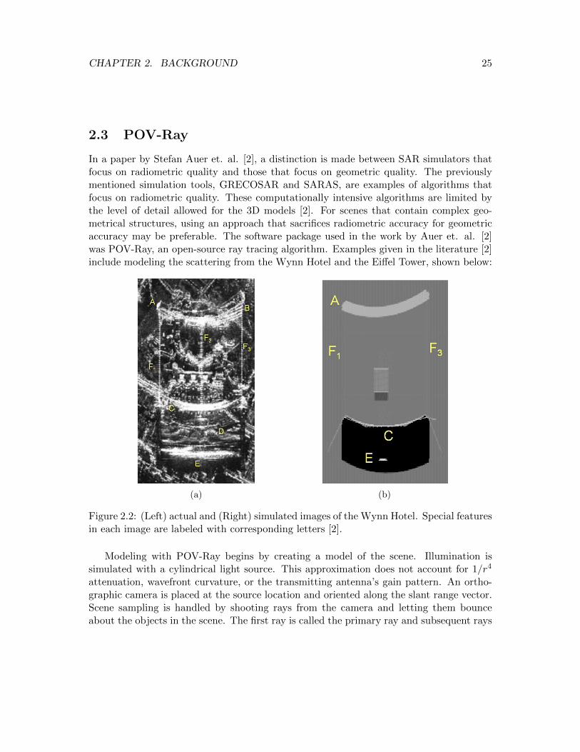
In a paper by Stefan Auer et. al. [2], a distinction is made between SAR simulators thatfocus on radiometric quality and those that focus on geometric quality. The previouslymentioned simulation tools, GRECOSAR and SARAS, are examples of algorithms thatfocus on radiometric quality. These computationally intensive algorithms are limited bythe level of detail allowed for the 3D models [2]. For scenes that contain complex geo-metrical structures, using an approach that sacrifices radiometric accuracy for geometricaccuracy may be preferable. The software package used in the work by Auer et. al. [2]was POV-Ray, an open-source ray tracing algorithm. Examples given in the literature [2]include modeling the scattering from the Wynn Hotel and the Eiffel Tower, shown below:
(a) (b)
Figure 2.2: (Left) actual and (Right) simulated images of the Wynn Hotel. Special featuresin each image are labeled with corresponding letters [2].
Modeling with POV-Ray begins by creating a model of the scene. Illumination issimulated with a cylindrical light source. This approximation does not account for 1/r4
attenuation, wavefront curvature, or the transmitting antenna’s gain pattern. An ortho-graphic camera is placed at the source location and oriented along the slant range vector.Scene sampling is handled by shooting rays from the camera and letting them bounceabout the objects in the scene. The first ray is called the primary ray and subsequent rays

CHAPTER 2. BACKGROUND 26
are called secondary rays. The contribution from each bounce is weighted by a reflectioncoefficient. For the sake of simplicity and to reduce computational complexity, the surfacereflectance was modeled as lambertian with a specular lobe. Next, the contributions fromeach ray are mapped to an azimuth and range coordinate. For each secondary ray, anadditional ray is created that is parallel to the primary ray but travels in the oppositedirection from the intersection point back towards the camera. The intersection of thisadditional ray with the camera is labeled the ray origin. The azimuth coordinate in theimage plane is calculated by taking the mean value of the azimuth coordinate for the ray’sorigin and the azimuth coordinate for the ray’s pixel location. Range is derived from thedepth value of the intersection point. The final output of the system is a reflectivity mapof the scene in azimuth and range coordinates. This output is obtained by superimposinga rectangular grid over the irregularly spaced returns from each ray and performing aninterpolation step.
Simulations were made on a skyscraper, the Wynn Hotel, and the Eiffel Tower. In manycases the brightness of the reflectivity map did not match well with the actual data. Thiswas especially the case along building edges where a significant diffracted return would beexpected, or at locations on the building’s surface that contained dihedrals/trihedrals notmodeled by the smoothed version in the ray tracing simulator. The main utility, however,was to be able to classify features in the reflectivity map by the number of bounces andthe macroscopic structures from which the signal was scattered. This improved imageinterpretability, as it identified why some features present in the SAR imagery, were absentfrom traditional overhead imagery taken by a camera.
2.4 DIRSIG
The Digital Imaging and Remote Sensing Image Generation (DIRSIG) tool is a physics-based ray-tracing algorithm used to model imagery across the electromagnetic spectrum forremote sensing applications [8]. Its ability to produce radiometrically accurate images forsingle-band, multi-spectral, and hyperspectral modalities is very well established. DIRSIGalso has a mature LIDAR modeling capability [8]. DIRSIG’s ability to model SAR imageryis still experimental at this stage. No work has been done that validates DIRSIG’s SARsimulation capability.
Being a ray-tracing algorithm, DIRSIG’s ability to model electromagnetic scatteringis limited to high-frequency approximation techniques. As will be shown in sections 3.2.3,3.2.6, and 3.2.7, ray-tracers, although treating light as a particle, can still model diffrac-tion using high-frequency techniques. Most imaging modalities traditionally modeled byDIRSIG at shorter wavelengths do not exhibit strong diffraction features and subsequently,no significant effort has been made to account for diffraction within DIRSIG. The addi-

CHAPTER 2. BACKGROUND 27
tion of these techniques adds another layer of computational complexity, especially whenimperfectly conducting surfaces or higher-order bounces are involved.
Modeling in DIRSIG starts with the creation of a scene. Scenes are usually built in theray tracing software Blender and a .ODB file is created. For each object ID in the scene,the material properties are specified in a .mat (material) file. The next step is to specify thepertinent system parameters and viewing geometry. For a traditional DIRSIG simulation,this can usually be done through a Graphical User Interface (GUI). To date, all of theseparameters have to be provided in xml tables as specified in the DIRSIG SAR ModalityHandbook [7]. DIRSIG then models the SAR return on a pulse-by-pulse basis. For a givenpulse, particles are shot into the scene from the transmitter using the LIDAR package. Insingle-pass mode, the receive computations are performed in the same pulse simulation asthe transmitted one. In two-pass mode, a hit map is created from the intersections, storedto file, and a separate simulation is run for the receive computations. Using two-pass modelessens numerical noise [7]. For each return, the transmitted waveform is convolved with adelta function delayed by the time-of-flight. The fast-time signal for a given pulse is thencreated by summing each of the returned waveforms. The amplitude of each return is alsoscaled by the Fresnel reflection coefficients. This is repeated for each pulse until the entiretime domain phase history for the user-defined collection is obtained.
There are a number of capabilities absent from DIRSIG normally found in a physicallybased SAR simulator. As mentioned earlier, DIRSIG uses the geometric optics approxi-mation and has no physical optics or edge diffraction modeling capability. Consequently,scattering is modeled using a Bi-directional Reflectance Distribution Function (BRDF),which is independent of target shape. This is adequate for rough-textured distributedtargets but not for smaller targets with smooth reflecting surfaces whose RCS is shape-dependent. An example would be the RCS for a small plate, which results in a 2D sincpattern that does not conform to a standard BRDF model. Options for the antennagain pattern are also limited to a few simple cases. Finally, transmitted waveforms arelimited to linear FM signals. Despite these limitations, and in some respects because ofthem, DIRSIG is still able to efficiently reproduce imagery in the radar modality withgood scene-wide qualitative agreement. This will be shown later in section 5.1. Addition-ally, with the way DIRSIG treats textured objects, Rayleigh distributed noise can also beobserved in the amplitude data, as expected. This will also be shown later in section 5.1.
The final output of DIRSIG is the complex phase history stored in an Envi .img file.This data can then be processed with user-defined code. It can also be processed usingRITSAR, a basic SAR image processing toolbox developed at RIT that is free and open-source and can be downloaded at www.github.com/dm6718/RITSAR.

CHAPTER 2. BACKGROUND 28
2.5 FDTD
Many of the approaches discussed thus far involve a high-frequency approximation for theincident field. In geometrical optics, this approximation is applied to the Luneberg-Klineseries. As shown in section 3.2.2, only the first term of this series is taken as a solutionto Maxwell’s equations in the high-frequency limit. This results in an eikonal equationwhich leads to the well known laws of reflection and refraction, as well as an additionalequation that accounts for amplitude loss with propagation and polarization effects. TheGeometrical Theory of Diffraction and Uniform Theory of Diffraction are extensions ofGeometrical Optics that describe how rays interact with edges, curved surfaces, and withthemselves, for example at a caustic. In physical optics, the high-frequency approximationleads to an assumption that non-uniform currents near an edge or shadow boundary canbe neglected. In both physical optics and the physical theory of diffraction, asymptoticforms of diffraction integrals are acquired by making a high-frequency approximation. Thispermits form solutions for diffraction coefficients without having to compute an integralfor each differential diffracting element.
All of the high frequency techniques above are only approximate solutions to Maxwell’sequations. All of these approximations become less accurate at low frequencies. Manyof them also do not take into account internal propagations [3] such as physical optics,which assume source currents are constrained to the surface. Obtaining an exact solutionto Maxwell’s equations can be practically impossible for arbitrary surfaces where theboundary conditions are difficult to implement in a natural coordinate system. In suchcases, where high-frequency techniques are insufficient, and exact closed form solutionscannot be obtained, numerical techniques are frequently used. The two most commontechniques are the Method of Moments [17] and Finite Different Time Delay (FDTD) [21].
The FDTD algorithm works by sampling a scene with a Yee lattice [21], creating asource, then modeling propagation by differencing the field in adjacent cells for a giventime step, as specified by the scalar rectilinear components of Maxwell’s curl equations.Boundary conditions are imposed by specifying the behavior of certain cells. For example,for a point on the surface of a conductor, the tangential E-field components are always0. The main drawback to this algorithm is the sampling requirements. In [3], the spatialsample spacing used was λ
10 . Even for manageable scene sizes, the temporal resolutionrequirements often result in thousands of time steps [3].
The utility of the FDTD algorithm for modeling urban scenes was investigated byDelliere et. al. [3]. The scene sizes were generally on the order of 10 m3 to 25 m3.Rather than model the signal from a complex scene, the paper focused on modeling howindividual canonical surfaces scatter light. This enabled simulations to be run in a rea-sonable time frame while still providing results that describe the backscattered signal of

CHAPTER 2. BACKGROUND 29
common objects in an urban scene. One of the canonical problems investigated was howperfectly conducting plates, with smooth or rough surfaces, scattered radiation. For thesmooth surface, the backscattered signal was dominated by diffraction peaks along theedges, whereas for rough surfaces, the signal was dominated by a speckle pattern whichappeared across the surface. The statistics of the speckle pattern followed a Rayleigh dis-tribution, as expected [3]. Below is a plot showing the field amplitude for both a smoothand rough plate:
Figure 2.3: Simulated amplitude of field reflected from both a smooth and rough plateusing FDTD [3].
The signal from a wall-ground interface was also investigated. The return showedmultiple peaks that correlated with the different orders of reflection that occur. Thelocation of the peaks from this last simulation matched well with what is predicted bygeometrical optics.

CHAPTER 2. BACKGROUND 30
2.6 Millimeter-wave Physical Optics Model
At Ka-band frequencies and higher, Bragg scattering features can be observed in a pow-erline’s RCS [22]. This is due to the fact that powerlines are normally comprised of anumber of cable strands which are tightly wound in a helical structure, which are peri-odic in nature. At certain aspect angles, adjacent rays reflected from this periodic surfaceconstructively interfere, leading to multiple orders of peaks in the RCS signature. Thelocations of these peaks are given by [4]:
θn = sin−1 nλ
2L(2.6)
Where n is an integer, θ is the aspect angle measured from a plane normal to the powerline’saxial direction, λ and 2L is the length of one period. The phenomenon that causes thesepeaks is the same as the one that gives rise to the Bragg diffraction pattern observedwhen x-rays are scattered from a periodic crystal lattice. Sarabandi, K. and Moonsoo,P. developed a way to compute the scattered field from powerlines using a method thataccounts for Bragg scattering [4]. This method uses an accurate powerline geometricalmodel, shown below:
Figure 2.4: Geometric powerline model used by Sarabandi, K. [4].

CHAPTER 2. BACKGROUND 31
The tangential component of the total magnetic field on the surface of the powerline in-duces source currents. These source currents can be computed from the incident magneticfield using an integral which can be evaluated numerically via the Method of Moments(MoM). The MoM is a technique which provides accurate results but is computationallyintensive at higher frequencies [4]. In order to efficiently evaluate the source current inte-gral without having to use MoM, a high-frequency approximation was made. This allowed
the source currents to be computed using a perturbation series instead of MoM. The 0th
order term in the series was the usual physical optics current given by J0 (r) = 2 (n×Hi).
Higher order terms were computed from this 0th order approximation using the pertur-bation series approach. The resulting nth order physical optics current was then used tocompute the scattered field using Green’s theorem. For periodic structures, a periodicGreen’s function was used and only one period of the powerline was needed for calculat-ing the scattered field. For non-periodic structures, such as powerlines with a significantamount of sag, the normal free space Green’s function was used and the entire lit portionof the powerline was needed for calculation instead of just one period.
This method was able to accurately simulate the RCS’s for a number of cables withvarious diameters and pitches within 20 about normal incidence for measurements takenat 94 GHz. The Bragg peaks in the simulated data lined up with those observed inthe measured data. Accuracy was degraded, beyond 20 about normal incidence, partlydue to surface irregularities not modeled in Figure 2.4. Additionally, the physical opticsapproach did not take into account the VV contribution from the grooves in the cable[23], resulting in increased error away from normal incidence for the VV channel. Beloware plots depicting how the simulated data compared to experimentally measured RCS’sfor a variety of powerlines:

CHAPTER 2. BACKGROUND 32
Figure 2.5: Simulated versus experimental RCS’s at 94 GHz for 4 different powerlines inthe VV channel. Bragg scattering peaks were accurately modeled by a PO approach atmillimeter wavelengths [4].
One of the primary drawbacks to using a physical optics approach is that the highfrequency approximation breaks down at X-band frequencies and lower for typical pow-erline diameters. Additionally, physical optics does not account for the VV contributionfrom the grooves observed in experiment [4, 6] and predicted by theory [23]. While theuse of MoM becomes more tractable for modeling powerline RCS’s at lower frequencies,it would still be difficult to implement this for a SAR application involving thousandsof pulses. For non-periodic powerline geometries with an appreciable amount of sag, theMoM approach would require calculations to be performed across the entire surface of thepowerline as opposed to just one period. This would include the non-lit regions for lowerfrequencies. Consequently, hardware requirements could be hard to fulfill for existingcommercial off-the-shelf desktops.
2.7 Xpatch
A well known RCS modeling toolkit used by the Air Force Research Labs (AFRL) and theDefense Advanced Research Projects Agency (DARPA) is Xpatch® [9]. Among Xpatch’sadvertised capabilities are modeling near-field and far-field scattering, rough surface scat-tering, and diffraction from an edge or point. According to the Xpatch website, diffraction

CHAPTER 2. BACKGROUND 33
is modeled using a Shooting and Bouncing of Rays (SBR) technique. As will be discussedlater in section 3.2.6, SBR is a high-frequency method which uses ray tracing to predictsource currents on a facet-by-facet basis. These source currents are then used to calculatethe contribution to the scattered field from the surface of a facet using physical optics(assuming far-field observation) and the contribution from an edge using PTD. In orderfor SBR to work, either the size of the facet has to be large enough or the bundle of rayshas to be dense enough for the incident field to be adequately sampled. This may not bepractical for optically thin wires or powerlines. Being a high-frequency technique, SBR isalso susceptible to errors in cases where the radius of curvature of the wire is too small.Generally, this is considered to be the case when the wavenumber-diameter product, k · a,is . 1 which is where this research is focused.
2.8 Summary
The techniques for simulating SAR imagery and RCS’s presented here each have uniquecapabilities. Examples of code that have been developed for the express purpose of beinga SAR simulator are GRECOSAR and SARAS. Software traditionally used for modelingimagery in the EO/IR regime such as DIRSIG and POV-RAY have also been adapted forefficient modeling in the radar modality. While computationally intensive, FDTD has alsobeen used to calculate the scattering from canonical targets for simple scenes, materials,and geometries. With respect to modeling powerlines, a physical optics based approachwas established for millimeter-wave radiation. Xpatch is another tool commonly usedfor radar modeling. This tool relies on SBR, a high-frequency approximation technique.Unfortunately, SBR breaks down for wavenumber-diameter products which are . 10.
Absent from many of the aforementioned methods are ways to incorporate the returnfrom thin cylindrical objects such as cables and power lines at X-band frequencies andlower. While GRECOSAR uses wedge ILDC’s to calculate the scattering from edges,there is no mention of a capability that models the diffracted return from thin cylindricalobjects. The original paper by Mitzner that derived the ILDC for wedges of various anglesalso contained the solution for thin cylindrical objects [10]. However, this does not appearto be incorporated into any current modeling tool. Work done by Sarabandi, K. andMoonsoo, P. did result in a numerical MoM based approach that could theoretically beapplied across all wavelength regimes, but would be practically difficult to implement forreal world powerline geometries given the current computational resources of commercialoff-the-shelf hardware.

Chapter 3
Theory
In this chapter, a discussion that focuses on the different ways to model electromagneticinteractions with matter are presented. At a top-level, an object’s RCS is often used todescribe how well the given object scatters power incident on its surface. The RCS is afunction of wavelength, angle of incidence, angle of observation, and the object’s materialand geometric properties. It can be derived from the radar range equation, which relatesthe power transmitted by an antenna to the power received at an antenna after the incidentradiation has scattered off an object. The RCS can also be expressed in terms of a ratio ofthe squared magnitude of the fields incident on the surface and scattered from the surface,as measured in the far-field. This latter definition enables the RCS to be computed fromfirst principles. This chapter begins with a formal definition of the RCS and then moves toa discussion of the different ways to model how objects scatter electromagnetic radiation.
Once traditional methods for modeling electromagnetic scattering have been reviewedand a common terminology established, the method used in this research to model power-line scattering is presented. This effort began with the creation of a physical model whichdefines the geometric and material properties of the powerline. Once these were estab-lished, the 2D problem of scattering into the forward cone (defined by Fermat’s principlefor Edge Diffraction, section 3.2.3) was solved. Work done by Mitzner [10] relates the 2Dsolution to the 3D scattering problem. It was shown that the 3D diffraction coefficientcan be expressed as a function of an Incremental Length Diffraction Coefficient (ILDC).For the special case of backscattering, this ILDC is equal to the 2D diffraction coefficient.Once the ILDC-based method for calculating the 3D diffraction coefficient was established,a number of follow-on activities were enabled. This included the simulation of powerlineRCS’s as well as the quad-polarization phase history for a SAR collection.
34

CHAPTER 3. THEORY 35
3.1 Radar Cross Section Definition
The radar range equation is commonly used to assess how well a given set of operatingparameters for a radar system can meet mission requirements. It relates the transmit-ted power to the received power through various loss and gain terms. The radar rangeequation, as defined in Ruck’s RCS Handbook, is given below [24]:
Pr =
(PtGtLt
)︸ ︷︷ ︸
Transmittingsystem
(1
4πr2tLmt
)︸ ︷︷ ︸Propagatingmedium
σ︸︷︷︸Target
(1
4πr2Lmr
)︸ ︷︷ ︸Propagatingmedium
(Grλ
20
4πLr
)︸ ︷︷ ︸Receivingsystem
(1
Lp
)︸ ︷︷ ︸
Polarizationeffects
(3.1)
where [24],
Pt = transmitter power in watts
Gt = Gain of the transmitting antenna in the direction of the target
Lt = numerical factor to account for the losses in the transmitting system
Lr = a similar factor for the receiving system
rt = range between the transmitting antenna and the target
σ = radar cross section
Lmt, Lmr = numerical factors which allow the propagating medium to have loss
r = range between the target and receiving antenna
Gr = gain of the receiving antenna in the direction of the target
λ0 = radar wavelength
Lp = numerical factor to account for polarization losses
When the transmitter and receiver are located on separate platforms, the collection ge-ometry is termed bi-static. When the transmitter and receiver are co-located (r = rt), thecollection is termed mono-static. Of particular interest for this research is the σ term inequation 3.1. This is the RCS of the target. The RCS is a commonly used metric thatdescribes how efficiently an object scatters radiation. Rearranging the range equation andsolving for σ yields the following expression [24]:
σ = 4πr2 4πPrLmrLpλ2
0Gr︸ ︷︷ ︸power densityscattered from
target
/PtGt
4πr2tLtLmt︸ ︷︷ ︸
power densityat target
(3.2)

CHAPTER 3. THEORY 36
The equation above is useful for measuring the RCS of a target in a lab. When calculatingthe RCS of a target from first principles, however, it is often more convenient to expressσ as a function of the incident and scattered fields rather than power. The power densityof electromagnetic radiation, W , is given by the following expression [25]:
W = Z0 (E ·E∗) /2 (3.3)
Where Z0 is the impedance of free space and E is the electric field vector (oriented alongthe polarization axis). Substituting this expression for the braced terms in equation 3.2,an alternate way of calculating σ is as follows:
σ = 4πr2 (Es ·Es∗)(Ei ·Ei∗)
= 4πr2 (Hs ·Hs∗)
(Hi ·Hi∗)(3.4)
where the i and s superscripts refer to incident and scattered fields, respectively. Atfirst glance, the equation above implies that the RCS is a function of distance. Thisis often undesirable since a more useful target metric would be one that is independentof the receiver distance and is solely dependent on target properties. One can achievesuch a metric by first noting the quantity (Es · Es∗) falls off as 1/r2 in the far-field [25].Consequently, the more widely used definition of the RCS, which does not depend onreceiver distance, is given as follows:
σ = 4π limr→∞
r2 (Es ·Es∗)(Ei ·Ei∗)
= 4π limr→∞
r2 (Hs ·Hs∗)
(Hi ·Hi∗)(3.5)
One way of interpreting this result is that σ can be thought of as “the area interceptingthe target that, when scattered isotropically, produces at the receiver a density that isequal to the density scattered by the actual target” [24]. Importantly, σ describes howefficiently a target scatters power but does not provide any insight into how a target affectsthe phase of the scattered field. Since SAR systems measure the phase of the scatteredfield, this will become important later on when methods for modeling how radiation isscattered from a power line are discussed.
3.2 Modeling Electromagnetic Propagation
There are a number of ways to model electromagnetic propagation. A recent paper byKravtsov, Y. and Zhu, N. provides a useful survey of the most common approaches usedin contemporary research [26]. Provided in this section is a more in-depth look at many ofthese approaches. First are Maxwell’s equations and some solutions that can be deriveddirectly from them. The case of perfectly conducting cylinders falls into this category. The

CHAPTER 3. THEORY 37
modeling of scattering from more complex objects using Maxwell’s equations, however, isoften too difficult to do analytically. The main issue with complex objects is the difficultyone has in applying boundary conditions to the scattering surface in a natural coordi-nate system. Numerical methods such as Finite Difference Time Delay (FDTD) [21] andMethod of Moments (MoM) [17] can be used for more complex surfaces. The drawback tothese methods is the spatial and temporal sampling requirements become onerous if thescene becomes too large or too complex [3]. Usually, approximations for the solutions toMaxwell’s equations need to be made. One such approximation is geometric optics (GO),the basis for essentially all ray tracing models. While GO does not fully take into accountthe wave nature of light, one can attach to each ray a ”payload” that keeps track of polar-ization, amplitude, and phase information as the ray travels through space and interactswith objects. In this way, one can account for some of the effects associated with the wavenature of light such as interference and polarization dependent reflection coefficients. GOworks well when the wavelength of light is much smaller than the characteristic length ofthe object. This approximation does not work well for describing how rays scatter off offeatures such as edges, tips, curved surfaces with small radii of curvature, and caustics.A solution is to use the Geometrical Theory of Diffraction (GTD) developed by Keller[27]. GTD essentially uses exact methods to determine ray amplitudes and what Kellerdescribes as Fermat’s Principle for Edge Diffraction to determine all the possible ray paths(and consequently, phases) for a given geometry.
In addition to geometric-based approaches for modeling electromagnetic propagation,there are also integral-based approaches. One such approach is physical optics (PO). Thefirst step in this approach is to estimate the surface currents on an object. Once the sur-face currents are known, a vector potential at the surface can be computed. This vectorpotential can then be used to calculate the observed scattered field at some observationpoint. This method is closely related to the Kirchhoff diffraction integral in scalar diffrac-tion theory. In both cases the Kirchhoff Approximation is used, which essentially assumesthe total field in the shadow region of a scattering object is zero whereas the total field inthe illuminated region is explicitly due to that of the incident field. This method is usuallymore accurate than GO since (1) it’s dependent on the frequency of radiation and (2) itpartially accounts for diffraction, the effect obstructions have on radiation, by filtering theangular spectrum of the incident radiation. PO does not, however, take into account per-turbations of the source field caused by the edges themselves. In this sense, the Kirkhoffapproach is not a complete method for modeling diffraction since it does not accuratelymodel the edge waves. PO works well when: the size of the object is sufficiently large suchthat the edge-diffracted waves are negligible when compared to the uniform componentwaves; the observation point is located in the far-field; and the surface of the object isconvex with a minimum radius of curvature much larger than a few wavelengths so that

CHAPTER 3. THEORY 38
the surface can be segmented into local tangent planes.In both GTD and PO, a singularity arises when computing the scattered field from
shadow boundaries for certain surfaces. Ufimtsev’s Physical Theory of Diffraction (PTD)[28] corrects this by subtracting the scattered field due to uniform currents (those predictedby PO) from the fields predicted by more exact solutions (GTD and the Sommerfieldsolution for scattering from a half plane), to obtain the scattered field solely due to non-uniform currents. The difference in the GTD and PO singularities is finite [25]. The mainlimitation with PTD is it only predicts the scattered field in what is termed the Kellercone [25], defined by Fermat’s Principle for edge diffraction [27]. For scattering directionsoutside the Keller cone, an extension of PTD developed by Mitzner which uses IncrementalLength Diffraction Coefficients (ILDC’s) can be used [25, 10].
The approximations to Maxwell’s equations described here are termed high frequencyapproximations. They are labeled as such since a high frequency approximation is madeto either neglect higher order terms in the Luneberg-Klein series solution to Maxwell’sequations (Geometric Optics) or to obtain analytic approximations for diffraction integralsusing a steepest descent or stationary phase method. While the wavelength of radaris much longer than that at optical regimes, these high frequency techniques still yieldaccurate results for many applications [25]. The main drawback to these techniques,however, is their inability to account for surface traveling (creeping) waves easily [25].While GTD makes allowance for these creeping waves, it does so only for simple shapes.Even with simple shapes, however, it is still possible for a creeping wave to make manyrevolutions around a closed surface, emitting radiation as it travels along. These higherorder emissions drastically increase the computational complexity. Efficiently modelingthe scattering due to creeping rays is an area of ongoing research [25].
While it may seem at first that the integral and geometric based approaches are exclu-sive to each other, much literature indicates otherwise. One example already covered isGTD, which uses exact solutions derived for canonical targets to determine the amplitudeof rays and Fermat’s Principle for Edge Diffraction to determine their phase. Anotherexample is the Modified Equivalent Current Approximation or MECA [29]. Presented inthe literature [30] is an extension of PO that is well suited for modeling the scattering ofdielectric materials using surface models that segment the object into triangular facets.Basically, GO (a ray tracer) is used to estimate the field incident on a facet by assumingeach intersection represented a plane wave having been incident on the surface. The Kir-choff Approximation is then used to derive the source currents. These in turn can then beused to derive a vector potential, at which point the Physical Optics integral can be usedto calculate the scattered field. For a triangular surface or facet, this integral has a closedform solution and the scattered field can be efficiently computed knowing only the anglesof incidence and observation, material properties (specifically the Fresnel reflection coeffi-

CHAPTER 3. THEORY 39
cients), and wavelength of radiation. A very similar approach is taken by the Shooting andBouncing of Rays (SBR) technique [31, 32]. In this method, rays incident on a surface cancome from both the source as well as from secondary reflections from other objects in thescene. Once the rays have propagated, the surface currents are approximated assumingplane wave incidence and a PO integral is evaluated to yield the final result.
3.2.1 Maxwell’s Equations
With very few exceptions, solutions to Maxwell’s equations represent the most accuratemodel for how electromagnetic radiation interacts with matter. The more accurate the-ory of Quantum Electro-Dynamics is usually more applicable to light-matter interactionproblems such as scattering from single atoms at resonant frequencies, the photo-electriceffect, and in the case of very strong fields, vacuum polarization resulting from electron-positron pair creation [33]. This research will investigate how light interacts with relativelymacroscopic objects whose work functions are much greater than the energy contained ina radar-wavelength photon. Consequently, the solutions to Maxwell’s equations will beconsidered the most accurate for the purposes of this research. Maxwell’s equations aregiven as follows:
∇ ·E =ρ
ε0(3.6)
∇ ·B = 0 (3.7)
∇×E = −∂B∂t
(3.8)
∇×B = µ0j +1
c2
∂E
∂t. (3.9)
While Maxwell himself did not derive the four equations above, he is credited with havingrecognized that they result in a wave equation:
∇2E− 1
c2
∂2E
∂t2=
1
ε0∇ρ+ µ0
∂j
∂t(3.10)
∇2B− 1
c2
∂2B
∂t2= µ0∇× j. (3.11)
In the absence of free charge and current (ρ = j = 0), equations 3.10 and 3.11 transforminto the vector Helmholtz equation:
∇2E + k20E = 0 (3.12)
∇2B + k20B = 0. (3.13)
CHAPTER 3. THEORY 40
with k20 = ω2/c2. The equations above can be solved by resolving the fields into their
vector components and solving the resultant scalar equations. Under certain constraints,the resulting scalar equations result in the scalar Helmholtz equation:[
∇2 + k20
]ψ(r) = 0 (3.14)
where an eiωt is suppressed and ψ(r) is a scalar field that can be related to the fields E, B,or as shown later a vector potential A, by a vector a such that E,B,A = aψ(r). One ofthe constraints required to go from the vector Helmholtz equation to the scalar Helmholtzequation is propagation through isotropic media, a condition automatically satisfied infree space. The other constraint is on the choice of the direction of a with respect to thecoordinate system used for the Laplacian operator ∇2. In rectangular coordinates, a canbe in any arbitrary direction [34]. In a spherical coordinate system, a must point in theradial direction [34]. For a cylindrical coordinate system, a must lie along the z-axis [34].In other words, analysis is restricted to TEz and TMz modes. This may seem restrictive atfirst glance. However, given that the TE and TM modes form an orthogonal basis and theincident and scattered fields in radar applications are usually linearly polarized, solutionscan be obtained by decomposition of the fields into the two basis vectors. When a cannotbe chosen to lie along one of the system’s coordinates, solutions to the scalar Helmholtzequation can still be used but specifying the boundary conditions becomes exceedinglydifficult. One example of scattering by a surface specified in prolate spheroidal coordinatesis given in [35]. In that paper, a was chosen to lie along one of the rectangular coordinates(TEx, for example). The incident field, originally specified in rectangular coordinates, hadto be decomposed into a sum of spheroidal wavefunctions so that the boundary conditionsin that coordinate system could then be specified and the solution for the scattered fieldobtained.
On the assumption the problem can be reduced to solving the scalar Helmholtz equa-tion, Green’s theorem can be used to transform the problem into an integral equation. Awell known example of this in the field of optics is shown later in section 3.2.4. Anotherapproach is to assume the solution is separable into three orthogonal coordinates ξ1, ξ2, ξ3:
ψ(ξ1, ξ2, ξ3) = ψ1(ξ1)ψ2(ξ2)ψ2(ξ2) (3.15)
For propagation through free-space, the solution is given as follows:
ψ(x, y, z) = ψ0e[i(kxx+kyy+kzz)] (3.16)
Another example is propagation through a rectangular waveguide. In this case, boundaryconditions need to be imposed, mainly that the field goes to 0 along the walls of therectangular prism. The result is a solution which has discrete wave numbers:
ψp,q(x, y, z) = ψ0e
[i(pk0x+qk0y+
√1−p2−q2z
)](3.17)

CHAPTER 3. THEORY 41
where p and q are integers.For infinitely long cylinders, the problem can be reduced to two dimensions by ex-
amining the solution at some point along the cylinder’s axis. In polar coordinates, thetwo-dimensional Helmholtz equation can be written as [36]:[
∇2 + k2]f =
1
r
∂
∂r
(r∂f
∂r
)+
1
r2
∂2f
∂θ2+ k2f = 0. (3.18)
Since we are working in cylindrical coordinates, f represents solutions for TEz or TMz
modes. After separation of variables with f = R(r)Θ(θ), and choosing −m2 to be theseparation constant for the θ coordinates, solutions to the polar two-dimensional Helmholtzequation are of the form [36]:
ψm(r, θ) =
∞∑m=0
[am cos(mθ) + bm sin(mθ)]Zm(kr) (3.19)
where Zm is any function that satisfies Bessel’s ODE [36]
r2 d2
dr2Zm(kr) + r
d
drZm(kr) + (k2r2 −m2)Zm(kr) = 0 (3.20)
Functions that satisfy the above ODE are Bessel functions of the first kind Jm(kr), Neu-mann functions Nm(kr), and Hankel functions Hm(kr) [36]. Any linear combination ofthese functions that satisfies the boundary conditions for a given problem may be used.The boundary conditions also specify the coefficients am and bm. This will become im-portant later in section 3.3.2 when the scattering of electromagnetic waves from cylindersis examined in detail.
3.2.2 Geometric Optics
One of the most common high frequency approximations to Maxwell’s Equations is that ofGeometrical Optics (GO). This approximation is also referred to as ray optics. Using thismethod, light propagation is modeled using bundles of rays that emanate from a source andinteract with objects. The direction of a ray is governed by Fermat’s principle. Applyingconservation of energy to a tube of rays yields amplitude information. Mathematically,GO is derived from the Luneberg-Kline series solution to the Helmholtz equation [34]:
E(R, ω) = e−ik0ψ(R)∞∑m=0
Em(R)
(iω)m(3.21)
Substituting this into the vector Helmholtz equation 3.12, applying the constraint ∇·E =0, and equating like terms yields the following sets of equations [34]:

CHAPTER 3. THEORY 42
1. Eikonal Equation
‖∇ψ‖2 = n2 (3.22)
2. Transport Equations
∂E0
∂s+
1
2
∇2ψ
n
E0 = 0 (3.23)
∂Em∂s
+1
2
∇2ψ
n
Em =
vp2∇2Em−1 (3.24)
m = 1, 2, 3 . . . (3.25)
3. Conditional Equations
s ·E0 = 0 (3.26)
s ·Em = vp∇ ·Em−1 (3.27)
m = 1, 2, 3 . . . (3.28)
where ψ is a surface which describes the wavefront, n is the index of refraction, s is theray distance, and s is normal to the wavefront ψ. The geometric optics approximation isrepresented by the 0th order term. This is called a high-frequency approximation sincehigher order terms in the Luneberg-Kline series, equation 3.21, are assumed to be negligi-ble. Equations 3.22 and 3.26 together are a representation of Fermat’s Principle, or morespecifically, Snell’s law and the law of reflection. Taking the first term of equation 3.21and substituting into the transport equation 3.23 yields the following result [34]:
E(s) = E′0(0)eiφ0(0)︸ ︷︷ ︸Field at reference
point (s=0)
√ρ1ρ2
(ρ1 + s)(ρ2 + s)︸ ︷︷ ︸Spatial attenuation
(divergence, spreading)factor
eiks︸︷︷︸Phasefactor
(3.29)
where ρ1 and ρ2 are the radii of curvature of the wavefront at some reference s = 0 and φ0
is the initial phase at the reference point. For a small spherical source located near s=0and choosing the location of the observation point to be far removed, the field amplitudeis proportional to 1/s. This conforms to the well known fact in radiometry that the powerfrom a point source is proportional to 1/s2. For scattering from an arbitrary surface and

CHAPTER 3. THEORY 43
incorporating Fresnel reflection coefficients, the resulting equation becomes [34]:
Er(s) = Ei(Qr)︸ ︷︷ ︸Field atreferencepoint (Qr)
· R︸︷︷︸Reflectioncoefficient
√ρr1ρ
r2
(ρr1 + s)(ρr2 + s)︸ ︷︷ ︸Spatial attenuation
(divergence, spreading)factor
eiks︸︷︷︸Phasefactor
(3.30)
where QR is a point on the surface of the scattering object and ρr is the radius of curvatureof the wavefront at the point Qr. For a spherical mirror, it can be shown that if the incidentfield is a plane wave, ρr = R/2 where R is the radius of curvature of the mirror [34]. Whens = −R/2 = f , where f is the focal length of the mirror, a singularity occurs in the spatialattenuation factor. This highlights a limitation of geometric optics for calculating the fieldat a caustic.
There are several limitations to using the geometric optics approach. For one, thespatial attenuation factor is independent of frequency. For some wavefronts, such as aGaussian, the spatial attenuation or divergence factor is strongly dependent on frequency.Using higher order terms in the Luneberg-Kline series will result in a more accurate so-lution. However, since it is usually difficult to work with these higher order terms, andthe resulting solutions still retain sharp discontinuities at shadow boundaries and do notaccount for diffraction, they are of limited use. Additionally, singularities occur at causticssuch as when s = −ρ. Nonetheless, geometric optics produce accurate results for manyapplications [34].
3.2.3 Geometric Theory of Diffraction
As shown, one of the main drawbacks to using GO is its inability to account for diffractedfields. The Geometrical Theory of Diffraction [27] extends GO by adding rays that diffractfrom an edge in addition to the normal rays that are reflected or transmitted from asurface. Much like how GO uses reflection and transmission coefficients to describe how theamplitude of a ray is attenuated by some surface interaction, GTD introduces diffractioncoefficients which describes how ray amplitudes are affected by an edge or by shadowboundaries. The direction rays travel is governed by Fermat’s principle for edge diffraction.This principle states that the path a ray travels from one point to another, with anintermediate point bound to the interacting surface, is that which has a stationary opticalpath. For scattering from surfaces, Fermat’s principle results in the law of reflection andSnell’s law. For diffraction, this results in a cone of rays rather than a single incident andscattered ray pair. This is because, unlike surfaces, edges are one-dimensional. This coneis sometimes termed the ”Keller cone.” Fermat’s principle for edge diffraction agrees well
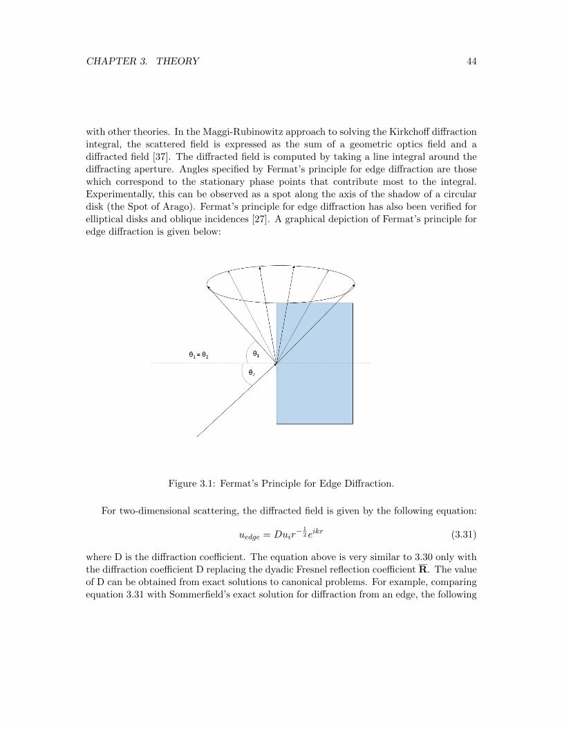
CHAPTER 3. THEORY 44
with other theories. In the Maggi-Rubinowitz approach to solving the Kirkchoff diffractionintegral, the scattered field is expressed as the sum of a geometric optics field and adiffracted field [37]. The diffracted field is computed by taking a line integral around thediffracting aperture. Angles specified by Fermat’s principle for edge diffraction are thosewhich correspond to the stationary phase points that contribute most to the integral.Experimentally, this can be observed as a spot along the axis of the shadow of a circulardisk (the Spot of Arago). Fermat’s principle for edge diffraction has also been verified forelliptical disks and oblique incidences [27]. A graphical depiction of Fermat’s principle foredge diffraction is given below:
Figure 3.1: Fermat’s Principle for Edge Diffraction.
For two-dimensional scattering, the diffracted field is given by the following equation:
uedge = Duir− 1
2 eikr (3.31)
where D is the diffraction coefficient. The equation above is very similar to 3.30 only withthe diffraction coefficient D replacing the dyadic Fresnel reflection coefficient R. The valueof D can be obtained from exact solutions to canonical problems. For example, comparingequation 3.31 with Sommerfield’s exact solution for diffraction from an edge, the following
CHAPTER 3. THEORY 45
expression for D is obtained:
D = − eiπ/4
2(2πk)12 sinβ
[sec
1
2(θ − α)± csc
1
2(θ + α)
](3.32)
where β is the angle between the incident ray and the edge and θ and α are the angles theincident and diffracted rays make with the surface normal, respectively. Note that whenλ → 0 (k → ∞), D goes to 0, as expected. Exact solutions can also be used to derivecorrection coefficients for fields at a caustic [27].
In addition to a straight edge, the diffraction coefficient for scattering from othercanonical surfaces can be derived in a similar manner. These include scattering from thetips of cones, pyramids, and from points on a curved surface tangential to the incidentrays. In the latter case, creeping rays result. This is because optical paths for tangentialrays which travel along a geodesic before heading in the scattered direction are stationary.In fact, a ray can make a number of revolutions around a surface resulting in higherorder creeping rays, although the amplitude decays exponentially with distance traveled[27]. Calculating the contribution from creeping rays can be difficult for canonical surfacesaddressed by GTD. For arbitrary surfaces, creeping ray calculations are an ongoing areaof research [25].
While GTD is more accurate than GO since it accounts for diffraction, there are still anumber of limitations. For one, GTD still relies on a high-frequency approximation. TheSommerfeld solution computes the scattered field by integrating the contributions from aspectrum of plane waves along the surface near the edge. In order to express Sommerfeld’ssolution in the form of equation 3.31, a steepest descent method assuming kr →∞ had tobe applied [37]. Additionally, the diffraction coefficients become singular along geometricshadow boundaries (such as when θ = α + π in equation 3.32). Although application ofthe residue theorem to the integral in Sommerfeld’s formulation leads to a finite result[37], the diffraction coefficients in GTD use the wide angle solution [25] which retainsthe singularities. This is addressed later by Ufimtsev’s Physical Theory of Diffraction(section 3.2.7) and also by the Uniform Theory of Diffraction [38]. Finally, GTD onlypredicts the amplitudes of rays that lie in the Keller cone. For finite surfaces, a spreadingof energy outside this cone can occur. Calculating the scattered field outside this conecan be accomplished using the closely related Incremental Length Diffraction Coefficients,discussed later in section 3.3.3.
3.2.4 Scalar Diffraction Theory
In addition to geometric or ray optics approaches to modeling electromagnetic scattering,there are also integral-based methods. Instead of starting with the Luneberg-Kline series,

CHAPTER 3. THEORY 46
these integral-based approaches start with the Helmholtz equation. Solutions to thisequation are obtained with the help of Green’s functions.
In this section, a brief review of scalar diffraction theory applied to a planar apertureis presented. This discussion will be useful later on when the closely related but moregeneral physical optics approach is discussed. As noted in section 3.2.1, there are certaincoordinate systems where the vector Helmholtz equation can be transformed into the scalarHelmholtz equation. The rectangular coordinate system is one of them. Fortunately, theproblem of a planar aperture can be treated naturally in this coordinate system. Below isa figure depicting an aperture located in the plane z = 0 and some of the variables thatwill be used in the remainder of this section:
Figure 3.2: Geometry for Scalar Diffraction (Kirchoff) Integral.
A common way of solving inhomogeneous linear differential equations in the form
Ly(x) = f(x) (3.33)
where L is a linear operator, is to first find a Green’s function which satisfies the equationLG(x, t) = δ(x− t) and has the same boundary behavior as the solution y(x) [36]. Using

CHAPTER 3. THEORY 47
the sifting property of the Dirac delta function, the solution is given by:
y(x) =
∫ b
aG(x, t)f(t)dt (3.34)
where a and b define the boundary [36]. This can easily be verified by applying L toboth sides and using the sifting property of the Dirac delta function. Equation 3.34 leadsto an important interpretation of the Green’s function G, mainly that it is the impulseresponse of the operator L. For example, let the source term in equation 3.33 be a deltafunction centered at x0: f(x) = δ(x − x0). Plugging this impulse into equation 3.34yields the solution y(x) = G(x, x0). The example just shown is one-dimensional, but theconcept can be extended to three dimensions also. While the scalar Helmholtz equation ishomogeneous (in other words, there is no source term from a mathematical standpoint),the Green’s function for the linear operator L = ∇2 + k2
0 can still be used to obtain asolution.
Let u(r) be the solution to the Helmholtz equation which satisfies the appropriateboundary conditions. For the present moment, let G(r, r′) be any scalar function. FromGreen’s theorem, the following condition holds [33]:∫
Ω
[u(r′)∇′2G(r′, r)−G(r′, r)∇′2u(r′)
]d3r =
∫Σ
[u(r′)∇′G(r′, r)−G(r′, r)∇′u(r′)
]· dS′ (3.35)
Now, let G(r, r′) be a Green’s function which satisfies the following equation [33]:[∇2 + k2
0
]G(r, r′) = −δ(r − r′). (3.36)
After some algebraic manipulations and noting that[∇2 + k2
0
]u(r) = 0, the left hand side
of equation 3.35 simplifies [33]:
u(r) =
∫Σ
[u(r′)∇′G(r′, r)−G(r′, r)∇′u(r′)
]· dS′. (3.37)
One function which satisfies 3.36 is given by [33]:
G0(r′, r) =exp(ik0|r − r′|)
4π|r − r′|. (3.38)
CHAPTER 3. THEORY 48
Equation 3.37 can be further simplified if G(r, r′) = 0 over the surface Σ in figure 3.2.This is also known as a Dirichlet boundary condition. Another way of expressing thisboundary condition is with the following equations [33]:
G(r′, r) = 0 when z′ = 0+ (3.39)
r′(∂G/∂r′ − ik0G
)= 0 when r′ →∞. (3.40)
When these two equations are satisfied, and assuming u(r′) also equals 0 when r′ → ∞,the integral in 3.37 reduces to the following [33]:
u(r) =
∫z′=0+
u(r′)∂
∂zG(r, r′)dS′. (3.41)
Here, we have used the fact that dS′ points in the z direction. Equation 3.38 satisfiesequation 3.39 but not 3.40. Using the method of images, an alternate Green’s functioncan be constructed that satisfies both 3.36 and the Dirichlet boundary condition. Thisalternate Green’s function is given by [33]:
G(r′, r) =exp(ik0|r − r′|)
4π|r − r′|− exp(ik0|r∗ − r′|)
4π|r∗ − r′|. (3.42)
Now, the second term in the integrand of equation 3.37 involving ∇′u(r′) is eliminated andthe solution simplifies even further to yield the Rayleigh-Sommerfeld diffraction integralof the first kind [33]:
u(r) = − 1
2π
∫z′=0+
u(r′)∂
∂z
[exp(ik0s)
s
]dS′. (3.43)
where s = r− r′ and s2 = (x− x′2) + (y − y′2) + z2. At this point, a few approximationsare normally made. The first is the Kirchoff approximation, which assumes the field inthe aperture region is exactly equal to the incident field, u(x, y, 0) = u0(x, y, 0) [33]. Usingthis approximation, the integral over the entire z′ = 0+ plane reduces to an integral overjust the aperture Σ. This approximation is valid when λ/a 1 where a is the size ofthe aperture [33]. It neglects, however, perturbations to u0 caused by the aperture itself.Another familiar result is the Fresnel diffraction integral, which can be obtained fromequation 3.43 by approximating s to second order. An even further simplification canbe made if the following criterion is met: k0r 1. If this condition is met, then theobservation point at r is said to be in the far-field. The far-field diffraction integral, alsoknown as the Fraunhoffer diffraction integral is given as follows [33]:
u(r) ≈ − ik0
2π
exp(ik0r)
r
∫aperture
u0(r′)exp(−ip · r′)dS′. (3.44)

CHAPTER 3. THEORY 49
Scalar diffraction theory cannot be applied to all scattering problems. As mentionedin section 3.2.1, there are few coordinate systems that support use of the scalar Helmholtzequation. For the planar aperture example given, it was straightforward to apply boundaryconditions to the Green’s function in rectangular coordinates. For arbitrarily shapedsurfaces, it is often more difficult to define the boundary conditions. Additionally, theKirchoff approximation neglects contributions from the edge of the aperture. These edgecontributions arise from what Ufimtsev terms non-uniform sources [39]. Neglecting thesecontributions can lead to large errors when the condition λ/a 1 is not met or when theobservation point is far from the geometrically illuminated region [25].
3.2.5 Physical Optics
In many applications, there is no easy way to describe the scattering surface in an or-thogonal coordinate system. Even when this is possible, there is no guarantee that thevector Helmholtz equation will result in at least one de-coupled scalar differential equationfor the coordinate system being used. For this, we will turn back to the wave equationand examine what simplifications and approximations can be made. For convenience, theelectromagnetic wave equations are restated below:
∇2E− 1
c2
∂2E
∂t2=
1
ε0∇ρ+ µ0
∂j
∂t(3.45)
∇2B− 1
c2
∂2B
∂t2= µ0∇× j. (3.46)
Previously, it was assumed there was no free charge or current. This assumption is mostlyvalid behind an opaque aperture, excluding points very close to the edges. Here, assumethat the radiation incident on the scattering object, which before was an aperture, pro-duces some surface current in the illuminated region but does not induce any current inthe shadowed region. Letting ρ → 0 and keeping the j term, equations 3.46 and 3.45become coupled in j. We can decouple these equations via a Lorentz gauge transforma-tion. Defining a vector potential A for the magnetic field, the following equations can bederived:
E = −∇φ− ∂A
∂tand B = ∇×A. (3.47)
After substitution of 3.47 into the wave equations 3.45 and 3.46 with ρ = 0, we have
∇2A− 1
c2
∂2A
∂t2= −µ0j. (3.48)
Now, the problem is simplified to merely finding solutions for equation 3.48, which isthe vector analog to the scalar inhomogeneous wave equation. Equation 3.48 is very
CHAPTER 3. THEORY 50
distinct from the scalar Helmholtz equation in the previous section, since now there isa source term, j, making the differential equation inhomogeneous. Before, the Green’sfunction was simply a mathematical tool used to obtain a solution to the homogeneousHelmholtz equation via Green’s theorem. Dirichlet Boundary conditions were imposed onthe Green’s function to simplify the problem and limit the assumptions made about theboundary conditions for u(r). The physical meaning of the resulting Green’s function (twopoint sources that were mirror images of each other) was abstract. Now with a sourceterm in equation 3.48, the forthcoming Green’s function has more physical significance. Itrepresents the contribution to the magnetic vector potential A due to a point of currentdensity j.
The objective at this point is to find an expression for the vector potential A. Usingthe technique introduced in 3.2.1, this vector equation can be solved by finding solutionsto its scalar equivalent, provided an appropriate coordinate system is used. Without lossof generality, a rectangular coordinate system will be assumed and analysis will proceed,using the scalar form of equation 3.48. For now, the only boundary condition to be appliedwill be the radiative boundary condition, mainly that the field goes to 0 as r→∞. Oncethis boundary condition has been imposed, we will return to the vector equations.
The scalar inhomogeneous wave equation is given by:[∇2 − 1
c2
∂2
∂t2
]ψ(r, t) = −f(r, t) (3.49)
Solutions for ψ(r, t) can be obtained by finding a Green’s function which satisfies thefollowing equation [33]:[
∇2 − 1
c2
∂2
∂t2
]G(r, t|r′, t′) = −δ(r− r′)δ(t− t′) (3.50)
It can be shown that the following function satisfies the equation above [33]:
G±(r, t|r′, t′) =1
4π|r− r′|δ(t− t′ ± |r− r′|/c) (3.51)
where the primed coordinates indicate the location of the source and the time the sourceexists, and the unprimed coordinates indicate the location of the observation point andthe time of observation. The Green’s functions G+ and G− represent advanced and re-tarded solutions, respectively. When using Green’s theorem to solve for ψ, the volume ofintegration is often evaluated in the limit V → ∞. This makes the advanced solution,representing an incoming wave from some external source, irrelevant. Using the retardedsolution and applying Green’s theorem, the following solution for ψ is obtained [33]:
ψ(r, t) =
∫V
[∫G(r, t|r′, t′)f(r′, t′)dt′
]d3r′ =
1
4π
∫V
f(r′, t− |r− r′|/c)|r− r′|
d3r′ (3.52)

CHAPTER 3. THEORY 51
where the sifting property of the Dirac delta has been used for the integral over time.Reverting to the vector representation of the problem, the following solution for A is asfollows [33]:
A(r, t) =µ0
4π
∫j(r′, t− |r− r′|/c)
|r− r′|d3r′. (3.53)
Now, an assumption will be made that the observation point is in the far field, r′ r.With this assumption, and knowing that A should go as 1/r in order to match the behaviorof the Green’s function, |r − r′| is approximated in the denominator as just r. For theargument of j, a binomial expansion of |r − r′| is performed. Taking terms up to secondorder, equation 3.53 can be simplified even further [33]:
A(r, t) =µ0
4πr
∫j(r′, t− r/c+ r · r′/c)d3r′ (3.54)
In most cases this work addresses time-harmonic fields. Taking the Fourier transform of3.54 with respect to time, letting k = (ω/c)r, and letting frequency be a parameter, thefollowing time harmonic potential can be derived [33]:
A(r|ω) =µ0
4π
eikr
r
∫j(r′|ω)e−ik·r
′d3r′ ≡ µ0
4π
eikr
rj(k|ω) (3.55)
where j(k|ω) is the three dimensional spatial Fourier transform of the function j(r|ω).For perfectly conducting objects, the j(r′|ω) term is only non-zero on the surface. Conse-quently, the volume integral becomes a surface integral and the final result on the right-hand side of 3.55 is the vector analog of the Fraunhofer diffraction integral.
The form of equation 3.55 given by Zangwill is especially useful when the scattering sur-face is illuminated by non-coherent illumination. It allows the vector potential A(r|ω) tobe computed through a Fourier decomposition of source terms. Essentially, the spectrumfor A(r|ω) can be built up from the monochromatic solutions on a frequency-by-frequencybasis. This is a widely used approach in optics [40]. Knowing that the solution for A(r, t)can be built up in the temporal frequency ω domain from the decomposed monochromaticsource terms, the parameter ω will be implicit for the remainder of this paper.
Thus far, the only approximation made to arrive at equation 3.55 is that the observationpoint is in the far-field. Now, two additional approximations will be made. The first is thetangent plane approximation. Assuming plane wave incidence on the surface and assumingthe surface can be locally approximated as planar (in other words, the radius of curvatureis large compared to the wavelength), then the surface current at the point r′ is given byµ0j(r
′, t) = 2n×Binc(r′, t) [33]. Additionally, the Kirchoff approximation will be made so
CHAPTER 3. THEORY 52
that there are no surface currents in the shadow region. Summarizing,
µ0j(r) =
2n×Binc(r) in illuminated region
0 in shadow region.(3.56)
When the incident wave is a plane wave, Binc = B0 exp(ik0 · r). Using this expression forB(r), collectively with equations 3.47, 3.55, and 3.56, the E field is given by:
E(r) ' iω
2π
exp[ikr]
rk×
k×∫S
(n′ ×B0) exp[i(k0 − k) · r′]dS′ (3.57)
The approximations used to arrive at this result, mainly the far-field, tangent plane, andshadow boundary approximations, are collectively termed the physical optics approxima-tion [24].
Another derivation of equation 3.57 often found in the literature is via the Chu-Strattonintegral. This is another integral form of Maxwell’s equations that does not use theLorentz gauge transformation or the vector potential A. Applying the physical opticsapproximation leads to the same results, however (5.10 in [25]).
The most obvious downside to using the physical optics integral is that it inaccuratelymodels currents near an edge or shadow boundary. For large structures, this usually isacceptable [24] since the contributions from non-uniform sources are greatly outweighed bythe uniform components. It can also be shown that the physical optics integral, equation3.57, does not produce any cross-polarization terms [25]. This is a result that conflictswith known experimental data [25]. Finally, the physical optics integral produces erroneousresults for observation points far removed from the specular direction [25].
3.2.6 Modified Equivalent Current Approximation
In the previous section, it was assumed that the scattering object was perfectly conducting.The Modified Equivalent Current Approximation (MECA) [29, 30] extends physical opticsby incorporating imperfectly conducting surfaces. The macroscopic forms of Maxwell’sequations for dielectric media are given by [34]:
∇×E = −M− µ∂H∂t
(3.58)
∇×H = j + ε∂E
∂t(3.59)
∇ ·E =ρ
ε(3.60)
∇ ·H = 0. (3.61)

CHAPTER 3. THEORY 53
The constants ε and µ are introduced to account for the material’s response to externalelectric and magnetic fields. The quantity H is an auxillary field related to the microscopicfield B by the following relation [33]:
H =1
µ0B−M =
1
µB (3.62)
The term magnetization is used to describe M. Physically, M represents a macroscopicmagnetic dipole density arising from a collection of point magnetic dipoles [33]. Thisdipole density can arise when an external magnetic field induces a preferred electron spinorientation or orbital state. Mathematically, M can also represent a virtual magneticcurrent that gives rise to a vector potential for E in much the same way that the currentdensity j gives rise the magnetic vector potential A. Consequently, M is often called themagnetic current density [34]. The term virtual is used to describe this current since thesecond of Maxwell’s equations, ∇ · B = 0, does not support the existence of magneticcharge.
Assuming no free electric charge, the wave equations for dielectric materials are [34]:
∇2E + k2E = ∇×M + µ∂j
∂t(3.63)
∇2H + k2H = −∇× j + ε∂M
∂t. (3.64)
Similar to what was done in the previous section, a vector potential for the field H willbe given by A. Additionally, a new vector potential will be introduced for the field E andwill be denoted by the quantity F. The fields can be derived from the vector potentialsusing the following equations [34]:
HA =1
µ∇×A EA = −∂A
∂t(3.65)
HF = −∂F∂t
EF =1
ε∇× F . (3.66)
Plugging these expressions into the dielectric wave equations results in the following in-homogeneous differential wave equations [34]:
∇2A + k2A = −µj (3.67)
∇2F + k2F = −εM. (3.68)
Using the same method presented in section 3.2.5, the following solutions for the potentials

CHAPTER 3. THEORY 54
A and M can be obtained from the source currents j and M [29]:
A(r) =µ
4π
eikr
r
∫j(r′)e−ik·r
′dS′ (3.69)
F(r) =ε
4π
eikr
r
∫M(r′)e−ik·r
′dS′. (3.70)
It is important to note that the equations above assume the source currents reside onthe surface. This assumption is valid if the material is thin and opaque such as for radar-absorbing paint. This is not the case in general for imperfectly conducting materials whichcan have bound currents throughout its volume.
E and H can now be calculated by using equations 3.65 and 3.66 which relate thefields to the potentials as well as equations 3.69 and 3.70 which relate the potentials to thesources. After some manipulation, the following equations provide the simplified relationbetween the fields and the vector potentials [34]:
E = EA + EF ' iω[−A + ηk× F
](3.71)
H = HA + HF ' iω[
1
ηk×A− F
]. (3.72)
The source terms in equations 3.69 and 3.70 can be approximated by using a physicaloptics approximation and incorporating Fresnel reflection coefficients [30]:
M = EincTE(1 +RTE)(eTE × n) + EincTM (1 +RTM )(k0 · n)eTE (3.73)
j =1
η
[EincTE(1−RTE)(k0 · n)eTE + EincTM (1−RTM )(n× eTE)
](3.74)
where eTE is a unit vector perpendicular to the plane containing k0 and the surface normal,n. For plane wave incidence, EincT () is the product of an amplitude term and a phase term
eik0·r′ that can be factored out of both the TE and TM terms. Using this knowledge, Mcan be re-written in the following form:
M = M0eik0·r′ (3.75)
where M0 is a vector which includes all the amplitude information. A similar processcan be applied to the current j. Concentrating on just M, the vector potential F can beexpressed in an alternate form to equation 3.70:
F(r) =ε
4π
eikr
rM0I(r) (3.76)

CHAPTER 3. THEORY 55
where,
I(r) =
∫ei(k0−k)·r′dS′. (3.77)
The term I is sometimes referred to as the re-irradiation diagram [16].This final expression is useful when a closed form for I can be obtained. This is true
when the surface is a triangular facet. Introducing new coordinates r′ = v01 +fv12 +gv13
where vmn is a vector which points from vertex m to vertex n, the integral I can now bere-written [30]:
I(r) = 2Ae−i(a+b/3)
1∫0
1−f∫0
ei(af+bg)dgdf (3.78)
where A is the area of the facet and:
a = kv12 · (r− k0) (3.79)
b = kv13 · (r− k0). (3.80)
The advantage of expressing the integral in this manner is that there are 5 possible closedform solutions to the integral I that correspond to 5 combinations of values for a and b[30]. Restricting a and be to be non-zero results in only two combinations [30]:
I(r) =
2A exp−ia+b
3
[a expib−b expia+b−a(a−b)ab
]a = b
2A exp−i2a
3
[ expia(1−ia)−aa2
]a 6= b
(3.81)
An important consequence of this result is it allows ray tracing software to be modifiedto efficiently calculate either the physical optics, or more generally, MECA solutions [29,30, 41]. This can be seen by first considering a single ray representing an incident planewave with some polarization. For a single intersection on the scattering surface withnormal n and Fresnel reflection coefficients specified by the material properties, all otherrequired parameters to compute the source currents, mainly k0, r, eTE, EincTE , and EincTM , areimmediately given. When the surface is broken up into triangular facets, these parameterscan be used to compute efficiently the vector potentials via 3.81 and, subsequently, thefields scattered in the direction r.
This approach is frequently found in the recent literature. It has been used as thebasis for a software tool that efficiently calculates the RCS’s of arbitrary objects [41]. Ithas also been used when assessing multiple scattering. Multiple scattering is handled byusing ray tracing software for all paths except the final one to the observer. Computationfor this final path is computed by using MECA for all intersections. This is referred toas the Shooting and Bouncing of Rays (SBR) technique and has been used to investigate
CHAPTER 3. THEORY 56
the RCS of cavities with a good degree of accuracy [31]. An implementation using theNVIDIA CUDA toolkit has also been implemented [32]. A software tool which uses MECAto simulate radar imagery [42] has also been developed by the companies ONERA andOKTAL. Information on the performance of this last tool is sparse in open literature butthe developers claim excellent agreement with real-world data [42].
Significantly, MECA similar limitations to those for the physical optics approximation.No allowance has been made here for edge currents. Consequently, there will be significanterrors in the scattered field away from specular observation angles just as with physicaloptics. Additionally, bound currents throughout the scatterer’s volume may exist forimperfectly conducting materials that would be unaccounted for in the surface integral.Unlike in physical optics, however, cross-polarization terms can be obtained from MECA.
3.2.7 Physical Theory of Diffraction
One of the main drawbacks with physical optics is the inaccurate results obtained forobservation points which are far from specular viewing angles [25]. For the case of scat-tering from a semi-infinite plane, the physical optics solution also contains singularities atthe geometric shadow boundaries. These singularities are similarly observed in the GTDdiffraction coefficients for geometric shadow transition regions [25]. Ufimtsev’s PhysicalTheory of Diffraction (PTD) seeks to correct this [28].
The most illustrative canonical problem in PTD is scattering from a semi-infinite halfplane or wedge. Ufimtsev hypothesized that the exact solutions given by Sommerfeldrepresent contributions from both uniform currents across the surface and non-uniformcurrents near an edge. The physical optics solution represents contributions from justthe uniform components. By subtracting the physical optics solution of scattering from asemi-infinite plane or wedge, from the exact solution, the only term remaining is that dueto non-uniform currents along the edge itself. Mathematically, this is expressed as [39]:
u(1) = u− u(0) (3.82)
where u(1) is the field due to edge (non-uniform) currents and is equal to the differencebetween u, the exact solution, and u(0), the field due to uniform currents predicted byphysical optics. While reference is made to non-uniform currents, no expression for themis ever provided in PTD. Expressions are only provided for the far-field scattered fieldsthat result from these currents. This is not relevant since it is the scattered field ratherthan the surface field that is of interest [25].
It turns out the singularities in the physical optics solution counterbalance those ob-served in the GTD diffraction coefficients which were derived from Sommerfeld’s solution.The result is diffraction coefficients that are non-singular, even along shadow boundaryregions, and agree well with experimental observation [25].

CHAPTER 3. THEORY 57
While the example given only addresses scattering from a semi-infinite plane or wedge,Ufimtsev also derived diffraction coefficients for other canonical shapes such as cones, disks,strips, ruled surfaces, and finite length cylinders [39]. In many cases, the semi-infinite half-plane problem was used as a starting point for deriving the diffraction coefficients for otherobjects. The approach is the same in all cases: mainly subtract the physical optics solutionfrom the exact solution to obtain the edge diffraction coefficients.
Ray tracing software and SBR is often used in conjunction with PTD (as well as GTD).Edges are identified as those lines which adjoin two adjacent facets whose difference infacet surface normals exceed some user defined threshold [12]. The facets adjoining theedge perform ray sampling for the edge. Directions for the outgoing rays are specifiedby Fermat’s Principle for Edge Diffraction and their amplitudes are given by the PTDdiffraction coefficients for the given wedge angle.
Thus far, no allowance has been made for imperfectly conducting material. Ufimt-sev provides a short discussion on how to approach calculating diffraction coefficients forimperfectly conducting surfaces [39] but these coefficients are not explicitly given. Addi-tionally, Ufimtsev’s theory only provides corrections for Keller’s GTD coefficients. Conse-quently, the PTD diffraction coefficients only describe the scattering of rays contained inthe Keller cone and provide no information on the rays scattered outside the Keller cone.For this, one can use the closely related Incremental Line Diffraction Coefficient (ILDC).
3.3 Power Line Modeling Using ILDC’s
Now that traditional methods for modeling electromagnetic scattering in the radar regimehave been reviewed, the approach formulated in the current research for modeling theradar return of powerlines will now be presented. This approach used a blend of using theexact solution to Maxwell’s equations for scattering from a perfectly conducting smoothcylinder and an extension of the Physical Theory of Diffraction that involves the use ofIncremental Length Diffraction Coefficients (ILDC’s). To begin, a physical model for thepowerline being modeled was created. This physical model described the shape as well asthe material properties of the powerline. These parameters were then used to calculatethe 2D solution for the scattered field. An ILDC approach was then used to extendthis solution to 3D, into the backscattering cone. Work done by Mitzner detailed howILDC’s can be used to extend 2D solutions to 3D [10]. In Mitzner’s report, a discussionwas provided on circular cylinder diffraction although an analytic form for the ILDC wasnever given [10]. Instead, this discussion on circular cylinder diffraction was used as astarting point to lead into edge diffraction. The most common application for ILDC’s isto compute how edges on a wedge scatter incident radiation. It was shown that the ILDCis equal to the 2D diffraction coefficient for the case of backscattering. In this research, a
CHAPTER 3. THEORY 58
2D ILDC was derived from the exact solution for scattering from an infinite length circularcylinder at oblique incidence. A 3D diffraction coefficient was then computed from thisILDC. The relationship between this 3D diffraction coefficient and the target RCS wasthen derived. This simulated RCS was later compared to experimental measurementsfor validation. The 3D diffraction coefficient was also used to simulate the SAR phasehistory for a powerline target. These results were compared to field data for a circularSAR collection. The sections below provide more details on the work entailed for eachstep.
3.3.1 Physical model
Before diffraction coefficients were calculated, a physical model needed to be establishedwhich took into account material and geometrical properties. To ensure efficiency wasachieved, the following assumptions were made:
1. The powerline insulation was transparent for the wavelengths being studied.
2. The material underneath the insulation was Perfectly Electrically Conducting(PEC).
3. The helically wound cables comprising the powerline were approximated as a singlesmooth cylinder for k · a . 1.
Since the powerline was not perfectly rigid, there was also be sag present in the geometry.Assuming a uniform mass density, the equation that described the shape of a suspendedcable was straightforward to derive. This was accomplished by finding the stationary valuefor the potential energy of the cable [43]. The potential energy V is given by:
V =
∫dm gy. (3.83)
where dm is a differential mass, y is the height of the differential mass, and g is gravitationalacceleration, assumed to be constant. Assuming a uniform mass density λ, a differentialelement of mass is related to a differential length of cable by dm = λds. plugging thisresult into 3.83 leads to the following sets of equations:
= gλ
∫yds (3.84)
= gλ
∫y√dx2 + dy2 (3.85)
= gλ
∫y√
1 + x2dy. (3.86)

CHAPTER 3. THEORY 59
Incidentally, this result matches the canonical problem of a minimum surface of revolutionin the calculus of variations. The infinitesimal variation of V, δV , is stationary when theintegrand satisfies the Euler-Lagrange equation [43]:
∂f
∂x− d
dy
(∂f
∂x
)= 0 (3.87)
Where f = y√
(1 + x2). Recognizing ∂f∂x = 0, and integrating with respect to y leads to
the following differential equation:
yx√1 + x2
= a (3.88)
dx
dy=
a√x2 − a2
(3.89)
The solution to this differential equation is that of a catenary, given by:
y = a coshx− ba
. (3.90)
where a and b are constants determined by the two endpoints. Below is a plot depictinga typical catenary curve:
Figure 3.3: Plot of a catenary.

CHAPTER 3. THEORY 60
3.3.2 2D Diffraction Coefficient
As shown earlier in section 3.2.1, the radial component of the solution to Maxwell’s equa-tions in cylindrical coordinates consists of Bessel functions. Imposing boundary condi-tions for a perfectly conducting cylinder and making the large argument approximationfor Bessel functions (the observation point is in the far-field), the particular solution atoblique incidence is given by [24]:
Es =
√2
πk0REi√
cos Ψ exp [i (k0z sin Ψ + k0R cos Ψ− π/4)]×∞∑
n=−∞(−1)nCn (3.91)
Where k0 is the carrier wavenumber, R is the distance from the cylinder to the observationpoint; Ψ is the obliquity angle; Cn is a quantity which depends upon polarization, cylindersize, and wavelength of radiation; and z is the distance along the cylinder from somereference point. The value z is assumed to be 0 for this research with no loss of generality.This is a 2D solution in that it only gives the field scattered into the forward cone Ψi =Ψs. Assuming a Perfectly Electrically Conducting (PEC) material, the constant Cn isdetermined by the wavelength of radiation and the diameter of the cylinder [24]:
CTMn = − Jn (k0a0 cos Ψ)
H(1)n (k0a0 cos Ψ)
(3.92)
CTEn = − J ′n (k0a0 cos Ψ)
H(1)′n (k0a0 cos Ψ)
(3.93)
CT ·n = CT ·−n (3.94)
Where Jn is an nth order Bessel function of the first kind, H(1)n is an nth order Hankel
function of the first kind, and the primes indicate derivatives. Assuming PEC material, thecross-polarization terms are 0. With equation 3.91, the 2D solution for the field scatteredinto the forward cone can be computed. The 2D RCS, also known as the scattering width,can be computed from this solution given the definition below [25]:
σ2D = limρ→∞
2πρ|Es|2
|Ei|2(3.95)
Below is a plot of σ2D versus the wave-number diameter product for both TE and TMradiation.

CHAPTER 3. THEORY 61
Figure 3.4: Plot showing the normalized 2D RCS of a circular cylinder for various radii atnormal incidence. The noisy signature at the end was caused by machine precision errorswhich arose when too many terms were used for the calculation. Physical optics would bethe preferable method in this high-frequency regime. The ‖‖ and ⊥⊥ subscripts refer toincident and outgoing TM and TE modes, respectively.
The Rayleigh regime is roughly characterized as the region where the TE scatteringcomponent functionally behaves like a small sphere and the TM component approachesinfinity with decreasing frequency [24]. As a side note, there is an asymptotic limit for theTM component, for as the frequency decreases past a certain point, the observation pointbecomes near-field [24] and equation 3.91 no longer holds. The resonance regime (alsocalled the Mie regime) is characterized by oscillation in the backscattering width of theTE component. The scattering width in the physical optics regime exhibits convergencebetween the two polarizations, with both scattering widths approaching the geometriccross-section for the case of backscattering at normal incidence.
An important quantity which can be derived from equation 3.91 is the dyadic 2Ddiffraction coefficient, d. This quantity relates the scattered field to the incident field as

CHAPTER 3. THEORY 62
follows [10]:
Es(R) = E01
cosβs√kR
eikRd · p. (3.96)
Combined with 3.91, the 2D diffraction coefficient for scattering from an infinite lengthcylinder at oblique incidence can be derived [10]:
d = 2
√2
πexp (−iπ/4)
∞∑n=0
(−1)n+1 Cn (3.97)
This quantity becomes important later when scattering in three dimensions is considered.
3.3.3 Incremental Length Diffraction Coefficient (ILDC)
Similar to the 2D diffraction coefficient in equation 3.91 which relates the field scatteredinto the forward cone to the incident field, a 3D diffraction coefficient can also be defined[10]:
D =1
2πexp [−i (2k · r + π/4)]kT sinc (X) d (3.98)
where T is the length of the cylinder, X is defined as kTπ sinβi, r is the distance from a
point on the powerline to a scene reference point, and βi is the obliquity angle for theincident field measured with respect to the axial direction of the cylinder. The quantity dis referred to as the Incremental Length Diffraction Coefficient and is in general a functionof the angle of incidence and the angle of observation. It was shown by Mitzner that theco-polarization ILDC for backscattering from PEC smooth cylinders is exactly equal tothe 2D diffraction coefficient for forward scattering [10]. Mitzner then goes on to showhow this can be computed using a physical optics based approach. For this research, d iscomputed using the exact solution given by equation 3.97 instead.
From the definition of the 3D RCS given by 3.4 as well as the definition of the 3Ddiffraction coefficient, equation 3.98, the following relationship between the two can bederived:
σ(θ) = λ2|npoints∑
i
Di(θ)|2 (3.99)
This equation is important later when this research is validated against experimentallymeasured powerline RCS’s.
3.3.4 SAR Phase History Simulation
Once the method for calculating the 3D diffraction coefficient was established, the SARphase history could be simulated. First, some conventions had to be established defining

CHAPTER 3. THEORY 63
the relationship between the polarization channels in the radar’s frame of reference andTE and TM components in the powerline’s frame of reference. The figure below depictshow these quantities were defined:
Figure 3.5: Depiction of the orientations of the polarization basis vectors from the aircraft’sframe of reference (H and V polarizations) and the powerline’s frame of reference (TE andTM polarizations). The definitions shown above were used to convert the polarizationamplitudes from one frame to another.
Simulation of the phase history was performed on a pulse-by-pulse basis usingRITSAR’s point simulator. The index for each pulse is denoted throughout with theindex j. The powerline itself was broken up into several small sections. The length ofeach section was chosen so there would be 2-3 sections within one resolution cell. Eachsection was then treated as a point and labeled with index i. Simulation of the phasehistory then proceeded using the following equation:
Sj(t) =
npoints∑i
Di,j exp(ik(t)Ri,j) (3.100)
where k(t) represents a linear FM wavenumber, Di,j is the 3D diffraction coefficient cal-culated for each powerline section, for each view using equation 3.98, and the dyad S

CHAPTER 3. THEORY 64
represents the quad-polarization phase-history. When calculating Di,j , the TE and TMcomponents were scaled by the projections of H an V onto these basis vectors for boththe incident and scattered paths. Additionally, it was assumed there was not enough sagin the powerline to induce a significant amount of cross-polarization signal, resulting ina diagonal S. The attenuation factor of 1/R2 was not included. This factor was approx-imated to be constant across the scene. Since this attenuation factor would have to becompensated for later when performing RCS comparisons, it was not deemed necessary toinclude it in equation 3.100.
3.4 Summary
Approaches for modeling electromagnetic scattering with a focus on radar wavelengthshave been presented. At a top level, the scattering problem can be described using theradar range equation, 3.1. The parameter of interest in this equation is the RCS whichprovides a measure of how efficiently a target scatters radiation in a given direction at agiven wavelength. The RCS also depends upon target material properties and shape but isindependent of observation distance, which makes this a useful metric. It can be calculatedusing equation 3.4, provided an expression which relates the scattered field amplitude tothe incident field amplitude is given. Common methods for deriving such an expressionwere also presented.
The most exact approach for calculating how electromagnetic radiation is scatteredfrom a target would be through application of Maxwell’s equations. This approach wasused to calculate the two-dimensional solution for scattering from a smooth cylinder. Thissolution was later used in calculating a 3D backscattering diffraction coefficient. In gen-eral, however, it is computationally inefficient to directly apply Maxwell’s equations whenmodeling the scattered signal from large, complex scenes. The oldest and most commonapproximation used is that of geometric optics. It can be shown that familiar princi-ples such as the laws of reflection, Snell’s law, and 1/r field attenuation can be derivedusing the first order approximation for the Luneberg-Kline series. Unfortunately, geomet-ric optics does not account for diffraction. The GTD can be used to extend geometricoptics by incorporating diffracted rays. This is done by creating rays that lie in whatis termed the “Keller cone” and are attenuated by a diffraction coefficient in much thesame way reflected rays are attenuated by a reflection coefficient. Although more accuratethan geometric optics, GTD is still limited to observation angles far from the geometricshadow boundary where singularities result and even then, only for rays contained in theKeller cone. Physical optics is a slightly more exact approach which originates from theintegral form of Maxwell’s equations. This form of Maxwell’s equations is also called theChu-Stratton integral. Using various assumptions collectively termed the physical optics

CHAPTER 3. THEORY 65
approximation, this integral can be simplified down to a form that is relatively easier toevaluate. As demonstrated in the literature, ray tracing approaches can be used as inputsto physical optics to estimate the sources for the scattered fields. In cases where the phys-ical optics integral can be evaluated analytically, diffraction coefficients can be derived.Much like the GTD diffraction coefficients, the physical optics diffraction coefficients resultin singularities near geometric shadow boundaries. Ufimtsev recognized that non-singulardiffraction coefficients can be obtained in this region by subtracting the physical opticssolution from the exact GTD solution (which in turn was derived from Sommerfeld’s exactsolution for scattering from a half-plane) to obtain the diffraction coefficient for just thenon-uniform edge currents. When this is done, the singularities near the shadow transi-tion regions offset each other in such a way as to yield a finite value for the diffractioncoefficient that matches well with experiment. Since PTD is an extension of GTD, it toois limited to the modeling of rays only contained in the Keller cone. For rays outside thiscone, Incremental Length Diffraction Coefficients (ILDC’s) can be used. These ILDC’sare closely related to the diffraction coefficients derived using PTD, GTD, and far-fieldapproximations to Maxwell’s equations.
In this research, the scattering of electromagnetic radiation was modeled using anILDC approach. First, a physical model was created which took into account geometricand material properties. Powerlines were approximated as smooth cylinders and their sagwas modeled using a catenary. Once the physical model was established, the 2D solutionfor scattering into the forward cone was calculated using Maxwell’s equations. From thissolution, an expression for the 2D diffraction coefficient was derived. It was shown thatthis value was equal to the backscattering ILDC for Mitzner’s 3D diffraction coefficient.An expression for the powerline RCS as a function of the 3D diffraction coefficient wasderived and used later on for validation. The 3D diffraction coefficient was also used tosimulate the powerline phase history for a SAR simulation.

Chapter 4
Methods
An assessment of DIRSIG’s ability to model both canonical targets as well as powerlineswas undertaken. This was performed using the AFRL Gotcha collection for the exper-imental data. The Gotcha dataset was particularly useful in that the scene containeda number of canonical targets that could be used for calibration. Being a circular SARcollection, it was also possible to process the data incrementally into smaller aperturesto extract multiple ‘frames’ that provided a 360 view of all objects in the scene, whichalso included powerlines. The assessment highlighted which objects in the AFRL scenecould be reasonably modeled using DIRSIG’s geometric optics-based approach and whichobjects required a more rigorous approach.
Validation of the ILDC approach was performed using a variety of datasets. The RCS’sof powerlines of various sizes and materials were measured in an anechoic chamber by theUniversity of Michigan. Both X and C band frequencies were used for the measurements.Since the diameter of the powerlines were on the order of a few centimeters, this placed thek · a value (k being the wavenumber and a being the diameter) squarely within the rangescoped by this research. Simulated data using Ufimtsev’s PO/PTD approach for finitecylinders were compared to simulated data generated, using an ILDC approach based onthe exact 2-D solution for backscattering from a finite cylinder.
In addition to the measurements taken in an anechoic chamber, powerline RCS’s werealso extracted from the AFRL Gotcha data. Unlike the powerlines in the anechoic mea-surements, these powerlines exhibited a significant amount of sag. This enabled the ILDCmethod to be evaluated for a geometry that would typically be found in field data.
66

CHAPTER 4. METHODS 67
4.1 Baseline DIRSIG Assessment
The primary source of data that was used for this research came from the AFRL Gotchacollection [5]. This data set consisted of the phase history and auxiliary information fora circular SAR collection of an urban scene using an X-band frequency and a bandwidthof 640 MHz. This scene included a parking lot, canonical calibration targets such astrihedrals and dihedrals, a grassy field, building, and powerlines. Images from this dataset were processed in 1 increments using 4 of aperture for each increment. The bulk ofthe modeled phase history for the Gotcha scene, minus power lines, was generated usingRIT’s DIRSIG. The approach taken for DIRSIG to model the SAR phase history is purelybased on geometric optics. The SAR functionality of DIRSIG is experimental at this stage.
DIRSIG’s ability to produce radiometrically accurate imagery is well validated in theoptical regime. To date, there have not been any attempts to validate the radar modal-ity. This research began with providing an initial assessment using data from the AirForce Research Labs (AFRL). This collection, labeled Gotcha, was particularly useful asit contained targets permitting calibration and it provided 360 of azimuth viewing an-gles, which enabled the extraction of parametric RCS’s. The goal was to demonstratewhere DIRSIG was deficient in modeling for the radar modality. It was hypothesized thatpowerlines would not be accurately modeled since their scattering cross section is muchlarger than their geometric one. The assessment included both a qualitative and quanti-tative comparison. The qualitative comparison involved visually inspecting the similaritybetween the simulated and experimental imagery. The quantitative comparison involvedextracting RCS’s for the canonical targets from the experimental imagery and comparingthem to the RCS’s extracted from the simulated DIRSIG data.
In order to simulate the phase history for the AFRL collection, a 3-D scene was builtin blender that roughly matched what was observed in the experimental data. The ex-perimental data contained canonical targets scattered throughout a field. Additionally,there were other features in the scene that contained objects commonly observed in urbanscenes such as buildings, a parking lot with cars, roads, and powerlines. Below are pro-cessed images of the AFRL SAR data using the backprojection algorithm for all 360ofazimuth:

CHAPTER 4. METHODS 68
(a)
(b)
Figure 4.1: Process imagery for Gotcha collection. (a) Total power image of AFRL dataproduced employing RITSAR using all 360 of azimuth for backprojection processing.Canonical targets appears as point sources in the top-left portion of the image. (b) Imageof view for which powerlines were apparent in the upper-right portion of image.

CHAPTER 4. METHODS 69
The canonical targets in the scene enabled some analysis to be performed on the data.Since the cross sections of the trihedrals and dihedrals have known theoretical values inall four polarization channels, they were used to calibrate the imagery. By isolating thesignature of the canonical targets for each viewing angle, RCS’s were derived from thedata. These RCS’s were then used for comparison to the RCS’s subsequently derived inDIRSIG simulations, enabling a quantitative comparison to be made. The figure belowshows the sizes and orientations of each of the canonical targets in the scene provided byAFRL/SNA:
Figure 4.2: Locations of canonical targets in the scene provided by AFRL/SNA [5].

CHAPTER 4. METHODS 70
Calibration of the imagery was performed using a backscatter correlation method [44].This method begins with the following signal model:
O = TSRᵀ +N (4.1)
Where O is 2x2 dyad containing the observed intensities in each of the four polarizationchannels, T and R are matrices that account for transmit and receive gains, respectively,N is the system noise and S is the desired calibrated scattering matrix for the scene wherethe value of each pixel is a measurement of the effective cross-section of all objects withinthe pixel. The first assumption made in the calibration process is that the transmitterand receiver gains remain constant throughout the collection. Next, it is assumed thatthe T and R matrices can be further broken down as follows [44]:
T = thh
(1 thvtvh 1
)(1 00 tvv
)≡ thhTΛT (4.2)
and similarly for R, where thh is a term which accounts for absolute gain, T accounts forpolarization impurity, and ΛT accounts for channel imbalance. Polarization impurity, ameasure of channel cross-talk (for example, if H and V are not perfectly orthogonal), wascomputed using the covariance matrix for a sub-image that contains scatters for which thefollowing assumptions can be made [44]:
1. The scatterers are reciprocal: shv = svh
2. There is no linear relationship between shh, svv, and svh (the correlation coefficientbetween channels 6= 1)
3. The system noise is uncorrelated with the scene scattering matrix
4. The noise covariance matrix = 0.
Natural scatters often have the qualities listed above to at least some degree. It wasassumed that a patch of grass in the Gotcha scene met the above criteria. Channelimbalance was then computed using the trihedral response knowing shh/svv = 1 andshv = svh = 0. Finally, absolute gain was computed using the known theoretical crosssection of the canonical targets. This information was then used to compute T and R inequation 4.2 and subsequently, to invert equation 4.1, yielding calibration factors for eachof the 4 polarization channels. On a decibel scale, these factors are actually offsets. Belowis a figure showing the calibration offset computed for each canonical target:

CHAPTER 4. METHODS 71
Figure 4.3: Plot showing the calibration offsets calculated using each of the canonicaltargets. Although the targets were of different sizes and types and placed at differentorientations, the calculated offsets were very similar. The range of the plot matches therange of the intensity scale for the raw image. The mean value indicated by the blue barrepresented the actual offset used.

CHAPTER 4. METHODS 72
Although the targets were of various shapes, sizes, and orientations, all yielded a verysimilar calibration factor.
In order to simulate the SAR phase history for this scene in DIRSIG, a number ofoperational parameters had to be extracted. Many were directly given in the MATLABstructure that accompanied the data. Many others, however, had to be inferred, basedon an assumption that the demodulated bandwidth of the de-chirped signal was approxi-mately equal to the transmitted pulse bandwidth. Below is a table summarizing the radarsystem parameters used in the DIRSIG simulation:
Table 4.1: AFRL platform parameters used for the DIRSIG simulation.
f0 9.6GHzchirprate 9.14× 10¹⁴ Hz/snsamples 424
A/D sampling rate 622 MHzbandwidth* 622 MHz
pulse duration* 681 nsrange resolution* 0.24 m
scene size* 100 m
*note: These are approximate values only. The bandwidth given is actually the intermediatefrequency bandwidth of the de-chirped signal, the pulse duration is actually the collection duration,and the range resolution is based on the intermediate frequency bandwidth. These are the valuesthat were used for the DIRSIG .platform file. Image quality was not adversely affected by usingthese assumptions for processing the phase history, indicating they are valid.
It was further assumed that the antenna gain pattern was a rectangular function inangular space with a half angle sufficient enough to ensure the entire scene was illuminated.More advanced gain patterns are not supported by DIRSIG. Also included in the MATLABstructure were the positions of the platform for each of the 8 passes recorded. Below is aplot of the flight path for each pass:
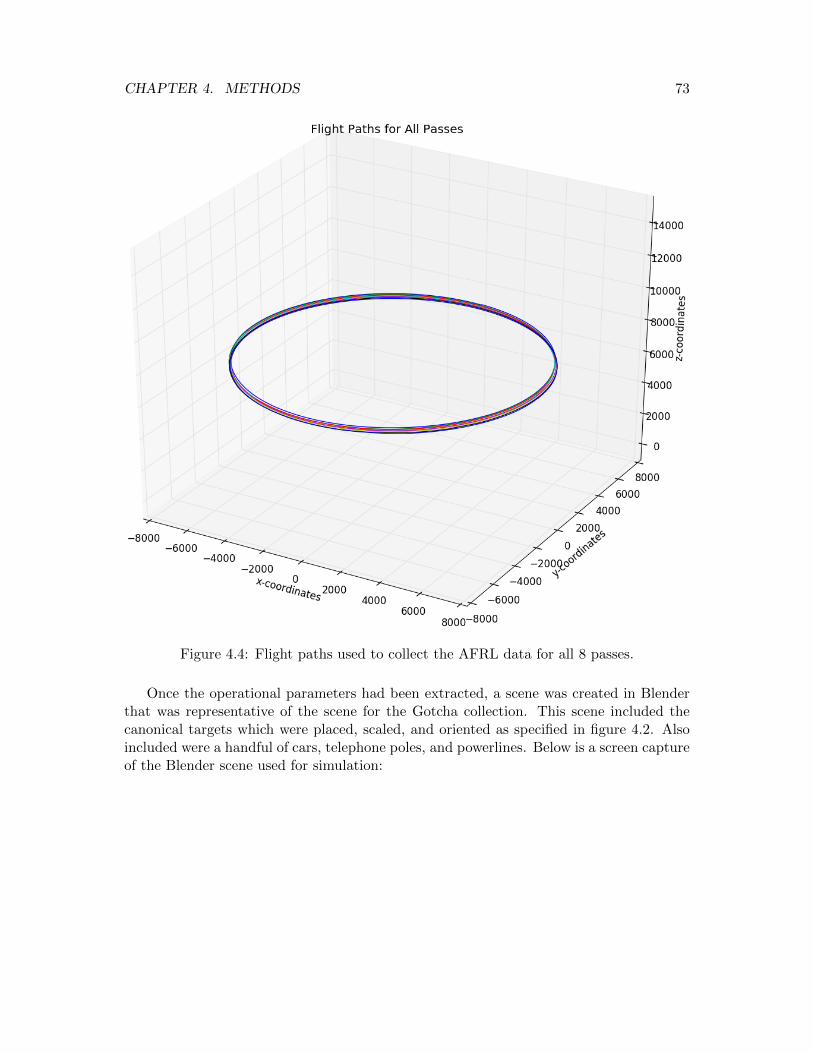
CHAPTER 4. METHODS 73
Figure 4.4: Flight paths used to collect the AFRL data for all 8 passes.
Once the operational parameters had been extracted, a scene was created in Blenderthat was representative of the scene for the Gotcha collection. This scene included thecanonical targets which were placed, scaled, and oriented as specified in figure 4.2. Alsoincluded were a handful of cars, telephone poles, and powerlines. Below is a screen captureof the Blender scene used for simulation:

CHAPTER 4. METHODS 74
Figure 4.5: Screen shot of Blender scene used for DIRSIG simulation.
The scene shown above is what was used for the qualitative assessment. Groundtruth for the reflectivity distributions was not obtained for any targets. Since the goalwas to perform a qualitative comparison between the simulated and field imagery for thescene-wide comparison, approximations for the reflectivity distributions were assumed tobe adequate for this purpose. For quantitative comparisons of the canonical targets areflectivity of one was assumed adequate. Since DIRSIG does not have a physical opticscapability, the reflectance distribution used was a simple specular lobe model. Realistically,the gain pattern for a perfectly conducting square surface would result in a 2D sinc patternwhose width would depend upon the dimensions of the surface. More specifically, thereflectivity model used in DIRSIG for all targets was described by the following equation:
BRDF (θi, θ0,∆φ) = d+ s ·MM(θn, n, k) · e−tan2θ
2σ2 . (4.3)
where s and d are the specular and diffuse reflectivity coefficients, respectively. For alltargets, σ was set to 0.1 radians. The reflectivities for each material contained in theDIRSIG scene are provided in the table below:

CHAPTER 4. METHODS 75
Table 4.2: Material reflectivity parameters used for the DIRSIG simulation.
material s d
grass 0.01 0.007asphalt 0.01 0.003
canonical targets 1.00 0.00vehicles 0.04 0.04
For the quantitative assessment, only the canonical targets were included in the scene.The resulting output was ‘calibrated’ using knowledge of the known input parameters suchas pulse power, pulse duration, and beam solid angle. The RCS’s of the canonical targetswere then extracted individually for subsequent comparison to the experimentally derivedRCS’s.
4.2 Power Line Modeling
In order to assess the viability of the method presented in this research, a number of datasources were used. The first source of data was graciously provided by the Universityof Michigan College of Engineering [6]. It included measurements of powerline RCS’s atdifferent frequencies for different cable diameters. These measurements were taken in acontrolled environment with well know truth data. The second source was the Gotchadata described in the previous section and provided by AFRL/SNA. The Gotcha dataenabled both a qualitative and quantitative comparison of field data. Powerline imagesextracted from the Gotcha data were used for qualitative comparison to the simulatedpowerline images. Powerline RCS’s extracted from the calibrated Gotcha data were alsoused for quantitative comparison to simulated RCS’s.
4.2.1 Anechoic Chamber Measurements
The accuracy of the ILDC approach presented in this research was first assessed usingdata collected in a controlled environment. This was accomplished by comparing thesimulated RCS’s of various types of powerlines to RCS measurements taken in an anechoicchamber. Below is a diagram depicting the overall setup for the experiment conducted bythe University of Michigan, College of Engineering [6]:

CHAPTER 4. METHODS 76
Figure 4.6: Depiction of the anechoic chamber setup from the Michigan experiment [6].
The scatterometer used to measure the backscattered return had a dynamic range of100 dB with quad-polarization capability. The antenna for this device consisted of a or-thomode transducer (OMT) and a dual polarized square horn with a cross-polarizationisolation of 20 dB [6]. Targets were placed on a styrofoam mount oriented by an azimuth-over-elevation positioner. Azimuth was controlled using a stepper motor that had a reso-lution of 1
10
and elevation was controlled using an analog positioner.
In order to calibrate the measured return to units of dBm2, a number of steps had tobe performed. First, 10 measurements of the Complex Amplitude (CA) of a calibrationsphere were taken over 10 viewing angles. Below is an image showing the sphere placedon a mount in the anechoic chamber:
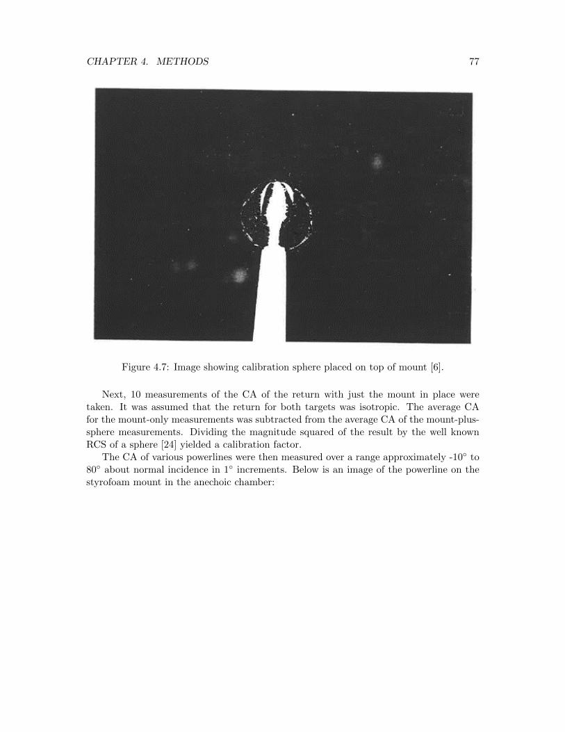
CHAPTER 4. METHODS 77
Figure 4.7: Image showing calibration sphere placed on top of mount [6].
Next, 10 measurements of the CA of the return with just the mount in place weretaken. It was assumed that the return for both targets was isotropic. The average CAfor the mount-only measurements was subtracted from the average CA of the mount-plus-sphere measurements. Dividing the magnitude squared of the result by the well knownRCS of a sphere [24] yielded a calibration factor.
The CA of various powerlines were then measured over a range approximately -10 to80 about normal incidence in 1 increments. Below is an image of the powerline on thestyrofoam mount in the anechoic chamber:

CHAPTER 4. METHODS 78
Figure 4.8: Image showing powerline placed on top of mount [6].
As with the calibration sphere, the average CA of just the mount was subtracted fromthe average CA of the mount plus powerline. The calibration factor computed using thecalibration sphere was then applied to the magnitude squared of the resultant data toyield measurements in units of dBm2. This was done for both X- and C-band frequencies.
The targets used in the experiment consisted of a variety of cables. In order to obtainfar-field measured data, the length of all cables was constrained to ≈ 1 ft. The geometriccross section of each target as viewed along the axial direction is shown below [6]:

CHAPTER 4. METHODS 79
(a)
(b) (c)
(d) (e)
Figure 4.9: Images depicting the geometric cross-section of each object for which RCSmeasurement were made: (a) 1.27 cm cylinder (b) 167.8 MCM Copper (c) 556.5 MCMAluminum (d) 954 MCM Aluminum & Steel and (e) 1431 MCM Aluminum & Steel. Allcables were ≈ 1 ft in length [6].

CHAPTER 4. METHODS 80
The powerline RCS’s measured as described above were used to validate the ILDCapproach presented in this research. The 3D diffraction coefficient of each of the targetsshown in figure 4.9 was simulated as described in section 3.3.3. These 3D diffractioncoefficients were then converted to RCS’s using equation 3.99. A comparison between thesimulated and measured RCS’s are presented in 5.2.1.
4.2.2 Gotcha Power Line RCS Comparison
In order to validate the method presented in this research against field data, the AFRLGotcha scene was used. A description of the Gotcha data set and how it was processedand calibrated is described in 4.1. Once the imagery was calibrated, the RCS’s of thepowerlines contained in the image were extracted. In order to extract the RCS of thepowerlines contained in the Gotcha image, a number of steps were performed. First, thetop 3 transmission lines were chipped from the full image for each frame. Below is animage of one of those chips:
Figure 4.10: Image chip of isolated transmission lines.

CHAPTER 4. METHODS 81
The bottom bundle of communication wires was not included. This bottom bundleof wires was closely spaced and since the method presented in this research does notsupport second order diffractions, a quantitative comparison with simulated data was notperformed. The RCS value for all pixels in the chipped image were summed to yield aneffective RCS of the entire chip. In order to compensate for the ground contribution, anearby patch of ground was also chipped from the image. The mean RCS of the groundchip was multiplied by the number of pixels in the power line chip, then subtracted fromthe power line chip. This yielded a measure of the effective RCS of just the top threetransmission lines in the image.
In order to simulate the RCS of the powerlines, a physical model was needed. Althoughexact ground truth of the power lines contained in the Gotcha scene could not be obtained,estimates based on visual inspection were used for developing the physical model. Belowis an image taken of a representative telephone pole:
Figure 4.11: Picture taken of a representative telephone pole configuration. The actualtelephone pole only had three transmission lines on top, configured similarly to what isshown in the picture, as well as a thick bundle of communication cables halfway up. Imagesof the actual telephone poles could not be obtained.

CHAPTER 4. METHODS 82
The configuration of transmission lines along the top of the pole are representative ofwhat was actually observed on-site. The transmission lines were approximately 2 cm indiameter and were modeled to have a 1.25 m drop over a 50 m run. Below the top threetransmission lines was a single bundle of approximately five communication cables. Thiscollection of cables was modeled for qualitative comparison purposes as a 50 cm diametercylinder with a 50 m run and 1 m drop. The 50 m run was measured directly from theGotcha images and the amount of sag was based on visual inspection and tweaked so thatscattering width of the main lobe in the simulated data matched that of the experimentaldata. Below are various plots depicting the physical model used:
(a)
(b) (c)
Figure 4.12: Physical model images. (a) Sketch of powerline in CAD software (b) 3Dpowerline plot (c) Side view of the top transmission line.

CHAPTER 4. METHODS 83
Once the physical model was built, the phase history for just the top three transmissionlines as well as the phase history for the transmission lines with communication cableswere simulated as described in section 3.3.4 using equation 3.100. The parameters listedin table 4.1 were used as input for the simulator. The phase history for a perfect pointreflector was also built and processed using the same parameters. The image of the perfectreflector was used for ‘algorithmic’ calibration to correct the gain induced by using thebackprojection algorithm as implemented in RITSAR. Once the impulse response of thepowerline images was corrected, each resolution cell provided a measure of the complex 3Ddiffraction coefficient. Applying equation 3.99 to each resolution cell and then summingall cells in the image yielded an effective RCS of the transmission lines, measured similarlyto the Gotcha data. These RCS’s were used for quantitative comparison. For qualitativecomparison, the phase history of the 3 transmission lines plus the bundle of communicationwires was simply added to the phase history of the DIRSIG Gotcha scene. Simulatedimagery was created using RITSAR to process the phase history.

Chapter 5
Results
In order to demonstrate the current capabilities and limitations of DIRSIG’s radar modal-ity, various comparisons were made. These comparisons provided a preliminary indicationof the current capabilities in this wavelength regime and highlighted where the geomet-ric optics approximation breaks down. Good scene-wide qualitative agreement with theGotcha field data was achieved. The amplitude noise distribution was also observed tobe Rayleigh distributed for both the simulated and field imagery, as expected. It wasalso demonstrated, however, that the geometric optics approximation was inadequate forsimulating the scattered return from the smaller canonical targets and the powerlines.
The ILDC method was designed to augment existing SAR modeling tools to accountfor the scattered return from powerlines. One of the ways in which this method wasevaluated was to compare predicted powerline RCS’s to those measured in an anechoicchamber. These measurements provided the opportunity to assess performance usingdata taken in a tightly controlled environment. A range of target types were used for theexperiment and measurements were taken using both X- and C-band frequencies. Giventhe constraints imposed by the physical dimensions of the chamber, the length of all targetswere kept to ≈ 1 ft in order to meet the far-field criterion for antennas df = 2L2
λ . Thisconstraint did not allow for the powerlines to sag by an appreciable amount. In orderto see how well the ILDC method worked for modeling powerlines as they would appearin a field-collected SAR image, comparisons were also made against the AFRL Gotchadata. As will be shown in the following sections, using the exact 2D ILDC for smoothcylinders provided an improvement over using a pure Physical Optics / Physical Theoryof Diffraction (PO/PTD) approach. The ILDC approach was also able to account for sagin the powerline for field collected data. A few discrepancies were noted, however. Adiscussion of possible causes for these discrepancies and how they may be accounted forin future work is discussed.
84

CHAPTER 5. RESULTS 85
5.1 DIRSIG Results
The SAR signal for the AFRL Gotcha scene was simulated as discussed in section 4.1. Theresultant phase history was processed into 357 “frames.” Each frame used 4 of azimuthfor processing with a starting azimuth ranging from 0 to 357 in 1 increments. Includedin the DIRSIG scene was the parking lot with cars, grassy field in the top portion ofthe image, canonical targets, and powerlines. Below is a comparison between a simulatedDIRSIG image and the corresponding actual Gotcha image:
(a) (b)
Figure 5.1: Qualitative Image Comparisons: (top) AFRL Gotcha, (bottom) simulated.
Both images appear to have good scene-wide qualitative agreement. Of note, however,is the absence of the powerline signature in the upper-right portion of the simulatedimage. The absence of a significant powerline signature was noted for all frames. This isa very strong validation of the statement that using a geometric optics approximation isinadequate for modeling powerlines in this wavelength regime.
Also of note is how well DIRSIG models speckle. The noise distribution for coherentimaging modalities follows a Rayleigh distribution [45]. In order to evaluate how wellboth the simulated and field data follow the theoretical noise distribution, a histogramfor a patch of grassy area was extracted. It was assumed that this grassy area could beadequately approximated as a flat field. The normalized histograms are shown below,along with a corresponding best fit Rayleigh distribution:

CHAPTER 5. RESULTS 86
(a) (b)
Figure 5.2: Intensity histograms for grassy field showing noise characteristics of data. Agood fit using a Rayleigh distribution was obtained for both the simulated DIRSIG dataand the Gotcha field data. This is consistent with the noise distribution expected forcoherent imaging modalities. (left) DIRSIG simulated, (right) Gotcha.
The fitting algorithm in SciPy’s stats.rayleigh module was used to generate the contin-uous curves shown above. The results in figure 5.2 show that amplitude noise for the fielddata is indeed Rayleigh distributed and that DIRSIG accurately models this phenomenon.As discussed in section 4.1, there was an absence of truth data for the reflectances of thedistributed targets in the scene, such as the grassy field. Since the purpose of the exercisewas to assess the level of qualitative agreement between the simulated and field imagery,approximations were used for the reflectance distribution functions. Consequently, thereis a mismatch between the mean and standard deviation for the observed and simulatedhistograms. Importantly, the results indicate that both histograms follow a Rayleigh dis-tribution.
The RCS’s for both the simulated and field measured canonical targets were extractedas described in section 4.1. The figures on pages 93-94 (figures 5.3 and 5.4) compare thetwo RCS’s to each other. The peak RCS for the canonical targets, depicted by the dottedgreen line in those figures, are given by the following equations:
σpeak =4πa4
3λ2(trihedral) (5.1)
σpeak =8π (w · h)2
λ2(dihedral). (5.2)
For the large 27 in. trihedral, DIRSIG came close to accurately modeling the return nearspecular incidence (0 phase angle in the RCS plots). Away from specular incidence,the simulated RCS diverges from the observed RCS for the 27 in. trihedral. For thesmaller trihedral targets, DIRSIG consistently underestimates the scattered return for all

CHAPTER 5. RESULTS 87
phase angles. This effect is especially pronounced for the dihedrals. The dihedral targetshave a low acceptance angle in elevation, and the side lobes in their field-measured RCSsignature indicate the need to use physical optics. For these targets, DIRSIG not onlyunderestimates the scattered return, but also fails to account for the side lobes since theRCS was modeled using geometric optics and a simple specular lobe reflectance model.A discussion of how physical optics has been implemented in other ray tracing softwareusing the shooting and bouncing of rays technique is provided in section 3.2.6. The focusof the current research, however, was on using an ILDC technique to model how powerlinesscatter radiation.

CHAPTER 5. RESULTS 88
(a) (b)
(c) (d)
Figure 5.3: RCS plots for trihedral targets: (a) TR1 (b) TR2 (c) TR3 and (d) TR4. Thetarget labels TR1-TR4 correspond to those in figure 4.2. The DIRSIG derived RCS’sconsistently underestimate the observed return, likely due to the absence of a physicaloptics capability.

CHAPTER 5. RESULTS 89
(a) (b)
(c) (d)
Figure 5.4: RCS plots for trihedral and dihedral targets: (a) TR5 (b) TR6 (c) DR2 and(d) DR6. The target labels TR5-DR6 correspond to those in figure 4.2.The DIRSIGderived RCS’s consistently underestimate the observed return, likely due to the absenceof a physical optics capability. This effect is especially pronounced for the dihedral targetswhich have small acceptance angle in elevation. Also absent in the simulated dihedralRCS’s are sidelobes, which require physical optics to be modeled.

CHAPTER 5. RESULTS 90
5.2 Power Line Modeling Results
The ILDC approach presented in this research was validated using two primary datasets.The first dataset was provided by the University of Michigan, College of Engineering [6].These data were collected as described in section 4.2.1 in a tightly controlled environ-ment. This allowed the ILDC method to be evaluated against measurements with limitedenvironmental contributions. Additionally, the configuration of target diameters and fre-quencies allowed an evaluation to be made with k · a products that ranged from 1.2 to 7,squarely within the range scoped for this research. Overall, error in the simulated RCSfell within the experimental uncertainty. The greatest discrepancy observed was for theX-band RCS of a 2.2 cm diameter cable (k ·a = 4.4) in the VV polarization channel. Thiswas likely caused by making the smooth cylinder approximation which does not accountfor the TE waveguide mode stimulated by V-polarization [6, 23].
In order ensure far-field measurements were being taken for the powerlines measured inthe anechoic chamber, their lengths were constrained to 1 ft. Consequently, an appreciableamount of sag was not present in the data. To see how sag affected the RCS signature,as well as to evaluate how well the ILDC method performed for a real-world scenario,powerline RCS’s extracted from the AFRL Gotcha field data were used. These RCS’swere obtained from the data using the process outlined in section 4.2.2. As with theanechoic data, significant error was observed in the VV channel. Additionally, 2nd orderdiffractions for the closely spaced transmission lines, which were not accounted for by themodel, may have also added to the error in the simulated data.
5.2.1 Anechoic Chamber Data
One approach for modeling finite length cylinders found in the literature combines PhyiscalOptics (PO) and the Physical Theory of Diffraction (PTD) [39]. For the cylindrical surfaceand the circular surfaces at each end, PO is used. For the edge adjoining the cylindricalsurface and endcaps, the PTD solution for a 90 wedge is used. When applying PO to afinite length cylinder and the endcaps, the following assumptions are made:
1. The observation point is in the far-field, df = 2L2
λ > 1, where L is the length of thecylinder and df is the observation distance.
2. The surface is locally flat k · a 1
3. No source currents are in the geometric shadow, including those which give rise tocreeping waves.
4. The target is Perfectly Electrically Conducting (PEC).

CHAPTER 5. RESULTS 91
Assumptions 2 and 3 in the list above are not valid for the data presented here. Addition-ally, the following assumptions and approximations are made when using PTD to modelthe edge contribution:
1. The surfaces adjoining the edge are locally flat k · a 1
2. Edge waves created by non-uniform source currents can be calculated accurately bysubtracting the PO solution for scattering from an infinite half-plane from Sommer-feld’s exact solution.
3. The contour integral along the edge can be efficiently evaluated by using a stationaryphase technique for only a handful of points.
Assumption 1 is once again invalid. When creeping waves are present, assumption 2 isalso invalid. Finally, the error associated with the approximation made in assumption 3is O (ka)−1 [39]. Alternatively, the ILDC method makes the following assumptions:
1. The observation point is in the far-field
2. Bragg scattering can be neglected
3. The semi-open waveguide signature for TE radiation incident on the grooves in thehelically wound cable can be neglected
4. The endcaps are not observed for real-world powerlines which will probably stretchbeyond the scene.
An advantage of using this method over a pure PO/PTD approach is that no restrictionis placed on k · a, although a practical one does exist if this product starts to approach100 when numerical machine precision is degraded, as shown in figure 3.4. Similarly,no assumptions are made about currents near a geometric shadow boundary or creepingwaves. The length of the powerlines for the anechoic measurements presented here wasconstrained in such a way to ensure a far-field measurement was made, ensuring assump-tion 1 was satisfied. For the AFRL Gotcha SAR imagery, the length of a segment ofpowerline contained within a resolution cell was also in the far-field. Assumption 2 wouldhave resulted in very distinct features that were not observed in the data. The literaturealso supports neglecting Bragg scattering for this k · a regime [4, 22]. Assumption 3 likelyresulted in error for data in the VV channel (with V polarization nominally aligned alongthe TE direction). Experiments in literature show that the VV signature away from nor-mal incidence can deviate from the smooth cylinder solution due to the TE waveguidesignature [6]. Finally, assumption 4 is arguably reasonable for field data where the ends ofthe powerlines likely extend past the scene boundaries. Since the length of the powerlines

CHAPTER 5. RESULTS 92
had to be constrained for the anechoic measurements to meet the far-field criterion, end-cap contribution dominated the signature away from normal incidence. Below are CADgenerated images of a finite length cylinder as viewed from different aspect angles:
(a) (b)
(c) (d)
Figure 5.5: View of finite cylinder at different aspects, as measured from plane normal toaxial direction: (a) 0 (b) 20 (c) 40 (d) 80. Note the increasing view of the endcap anddecreasing view of the cylindrical portion.
While the ILDC model does not account for endcaps, their contribution as predicted byPO/PTD was added to the ILDC signature so a reasonable comparison with the anechoicdata could be made.
The following pages show how the simulated RCS’s compared to the measured datafor a variety of targets at X-band frequencies:

CHAPTER 5. RESULTS 93
(a) (b)
(c) (d)
Figure 5.6: Modeled X-band power line RCS compared to anechoic chamber measurementsfor 1.27 cm diameter (ka = 2.5) smooth cylinder: (top-pair) using Physical Optics andPhysical Theory of Diffraction exclusively (bottom-pair) using exact smooth cylinder 2-D diffraction coefficient for cylindrical portion and PO/PTD for endcaps (left-pair) HHchannel (right-pair) VV channel. Error bars on the measured data are scaled by ± 1standard deviation. For the simulated data, error bounds depict the O (k · a)−1 errorassociated with using a stationary phase technique to evaluate the contour integral alongthe edge adjoining the endcap and cylinder.
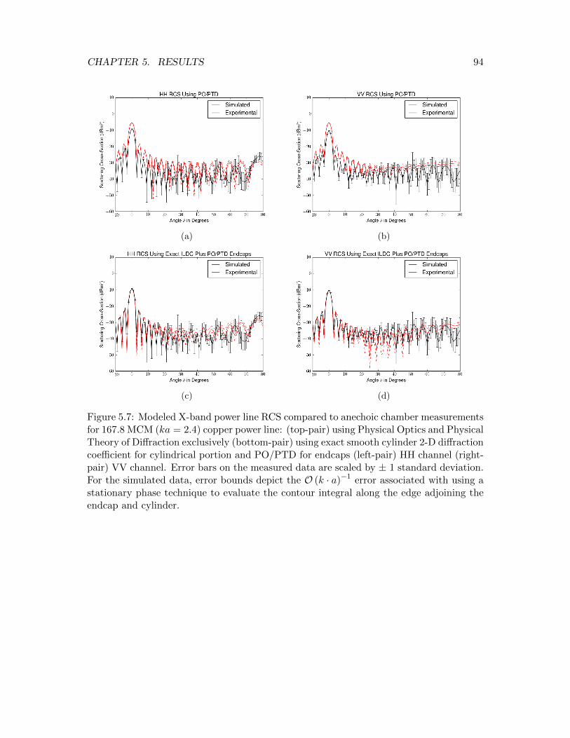
CHAPTER 5. RESULTS 94
(a) (b)
(c) (d)
Figure 5.7: Modeled X-band power line RCS compared to anechoic chamber measurementsfor 167.8 MCM (ka = 2.4) copper power line: (top-pair) using Physical Optics and PhysicalTheory of Diffraction exclusively (bottom-pair) using exact smooth cylinder 2-D diffractioncoefficient for cylindrical portion and PO/PTD for endcaps (left-pair) HH channel (right-pair) VV channel. Error bars on the measured data are scaled by ± 1 standard deviation.For the simulated data, error bounds depict the O (k · a)−1 error associated with using astationary phase technique to evaluate the contour integral along the edge adjoining theendcap and cylinder.

CHAPTER 5. RESULTS 95
(a) (b)
(c) (d)
Figure 5.8: Modeled X-band power line RCS compared to anechoic chamber measurementsfor 556.5 MCM (ka = 4.4) aluminum power line: (top-pair) using Physical Optics andPhysical Theory of Diffraction exclusively (bottom-pair) using exact smooth cylinder 2-D diffraction coefficient for cylindrical portion and PO/PTD for endcaps (left-pair) HHchannel (right-pair) VV channel. Error bars on the measured data are scaled by ± 1standard deviation. For the simulated data, error bounds depict the O (k · a)−1 errorassociated with using a stationary phase technique to evaluate the contour integral alongthe edge adjoining the endcap and cylinder.

CHAPTER 5. RESULTS 96
(a) (b)
(c) (d)
Figure 5.9: Modeled X-band power line RCS compared to anechoic chamber measurementsfor 954 MCM (ka = 6.1) steel & aluminum power line: (top-pair) using Physical Opticsand Physical Theory of Diffraction exclusively (bottom-pair) using exact smooth cylinder2-D diffraction coefficient for cylindrical portion and PO/PTD for endcaps (left-pair) HHchannel (right-pair) VV channel. Error bars on the measured data are scaled by ± 1standard deviation. For the simulated data, error bounds depict the O (k · a)−1 errorassociated with using a stationary phase technique to evaluate the contour integral alongthe edge adjoining the endcap and cylinder.

CHAPTER 5. RESULTS 97
(a) (b)
(c) (d)
Figure 5.10: Modeled X-band power line RCS compared to anechoic chamber measure-ments for 1431 MCM (ka = 7.0) steel & aluminum power line: (top-pair) using PhysicalOptics and Physical Theory of Diffraction exclusively (bottom-pair) using exact smoothcylinder 2-D diffraction coefficient for cylindrical portion and PO/PTD for endcaps (left-pair) HH channel (right-pair) VV channel. Error bars on the measured data are scaled by± 1 standard deviation. For the simulated data, error bounds depict the O (k · a)−1 errorassociated with using a stationary phase technique to evaluate the contour integral alongthe edge adjoining the endcap and cylinder.

CHAPTER 5. RESULTS 98
The Rayleigh far-field criteria for the measured data was:
df =2L2
λ= 5.9m. (5.3)
Since measurements were taken at 13 m, the observation point was in the far-field. Asummary of the results are provided in the table below:
Table 5.1: X-band results summary.
20 half-width about normal total
% error % uncertainty % error % uncertaintysimulated vs. between simulation vs. between
measured measurements measured measurements
Cylinder 1 HH 2.9% 5.2% 5.5% 10.2%Cylinder 1 VV 0.76% 2.0% 2.8% 10.1%
Cable 1 HH 1.2% 5.8% 4.4% 9.8%Cable 1 VV 2.4% 3.5% 1.8% 10.4%Cable 2 HH 3.3% 4.5% 8.6% 7.3%Cable 2 VV 29.5% 8.5% 15.7% 9.1%Cable 3 HH 5.3% 5.0% 3.3% 8.7%Cable 3 VV 9.5% 7.3% 6.3% 8.1%Cable 4 HH 2.4% 5.4% 8.4% 9.9%Cable 4 VV 2.4% 8.4% 3.1% 11.3%
mean HH 3.0% 5.2% 6.0% 9.2%mean VV 8.9% 5.9% 5.9% 9.8%
mean 6.0% 5.6% 6.0% 9.5%
Overall, accuracy was within the experimental uncertainty of the data. In all cases, theILDC approach performs better than the PO/PTD solution. Accuracy for the simulatedVV data, especially for Cable 2, did not perform as well as the HH data. This is likelyassociated with error inherent in making a smooth cylinder approximation for grooved,helically wound powerlines.
The figures on the following pages demonstrate how well the simulated RCS’s matchedthe measured RCS’s for the C-band data:

CHAPTER 5. RESULTS 99
(a) (b)
(c) (d)
Figure 5.11: Modeled C-band power line RCS compared to anechoic chamber measure-ments for 1.27 cm diameter (ka = 1.3) smooth cylinder: (top-pair) using Physical Opticsand Physical Theory of Diffraction exclusively (bottom-pair) using exact smooth cylin-der 2-D diffraction coefficient for cylindrical portion and PO/PTD for endcaps (left-pair)HH channel (right-pair) VV channel. Error bars on the measured data are scaled by ±1 standard deviation. For the simulated data, error bounds depict the O (k · a)−1 errorassociated with using a stationary phase technique to evaluate the contour integral alongthe edge adjoining the endcap and cylinder.
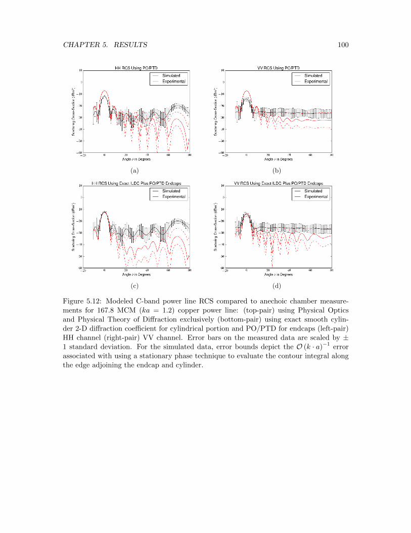
CHAPTER 5. RESULTS 100
(a) (b)
(c) (d)
Figure 5.12: Modeled C-band power line RCS compared to anechoic chamber measure-ments for 167.8 MCM (ka = 1.2) copper power line: (top-pair) using Physical Opticsand Physical Theory of Diffraction exclusively (bottom-pair) using exact smooth cylin-der 2-D diffraction coefficient for cylindrical portion and PO/PTD for endcaps (left-pair)HH channel (right-pair) VV channel. Error bars on the measured data are scaled by ±1 standard deviation. For the simulated data, error bounds depict the O (k · a)−1 errorassociated with using a stationary phase technique to evaluate the contour integral alongthe edge adjoining the endcap and cylinder.
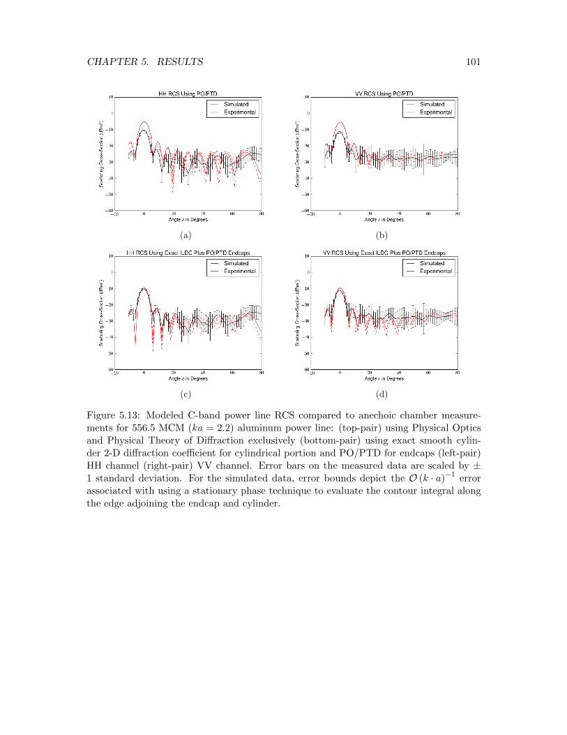
CHAPTER 5. RESULTS 101
(a) (b)
(c) (d)
Figure 5.13: Modeled C-band power line RCS compared to anechoic chamber measure-ments for 556.5 MCM (ka = 2.2) aluminum power line: (top-pair) using Physical Opticsand Physical Theory of Diffraction exclusively (bottom-pair) using exact smooth cylin-der 2-D diffraction coefficient for cylindrical portion and PO/PTD for endcaps (left-pair)HH channel (right-pair) VV channel. Error bars on the measured data are scaled by ±1 standard deviation. For the simulated data, error bounds depict the O (k · a)−1 errorassociated with using a stationary phase technique to evaluate the contour integral alongthe edge adjoining the endcap and cylinder.

CHAPTER 5. RESULTS 102
(a) (b)
(c) (d)
Figure 5.14: Modeled C-band power line RCS compared to anechoic chamber measure-ments for 954 MCM (ka = 3.0) steel & aluminum power line: (top-pair) using PhysicalOptics and Physical Theory of Diffraction exclusively (bottom-pair) using exact smoothcylinder 2-D diffraction coefficient for cylindrical portion and PO/PTD for endcaps (left-pair) HH channel (right-pair) VV channel. Error bars on the measured data are scaled by± 1 standard deviation. For the simulated data, error bounds depict the O (k · a)−1 errorassociated with using a stationary phase technique to evaluate the contour integral alongthe edge adjoining the endcap and cylinder.

CHAPTER 5. RESULTS 103
(a) (b)
(c) (d)
Figure 5.15: Modeled C-band power line RCS compared to anechoic chamber measure-ments for 1431 MCM (ka = 3.5) steel & aluminum power line: (top-pair) using PhysicalOptics and Physical Theory of Diffraction exclusively (bottom-pair) using exact smoothcylinder 2-D diffraction coefficient for cylindrical portion and PO/PTD for endcaps (left-pair) HH channel (right-pair) VV channel. Error bars on the measured data are scaled by± 1 standard deviation. For the simulated data, error bounds depict the O (k · a)−1 errorassociated with using a stationary phase technique to evaluate the contour integral alongthe edge adjoining the endcap and cylinder.
The Rayleigh far-field criteria for the measured data was:
df =2L2
λ= 2.9m. (5.4)
Since measurements were taken at 13 m away, the observation point was in the far-field.A summary of the results is provided in the table below:

CHAPTER 5. RESULTS 104
Table 5.2: C-band results summary.
20 half-width about normal total
% error % uncertainty % error % uncertaintysimulated vs. between simulation vs. between
measured measurements measured measurements
Cylinder 1 HH 14.5% 11.1% 31.9% 9.9%Cylinder 1 VV 4.2% 10.5% 2.4% 13.3%
Cable 1 HH 19.5% 14.3% 45.8% 15.2%Cable 1 VV 18.5% 15.6% 26.2% 14.0%Cable 2 HH 4.5% 11.4% 4.7% 15.1%Cable 2 VV 3.9% 16.8% 3.5% 16.6%Cable 3 HH 5.8% 9.4% 0.2% 15.0%Cable 3 VV 1.2% 12.7% 0.3% 16.3%Cable 4 HH 7.7% 6.0% 1.7% 11.3%Cable 4 VV 1.9% 12.1% 1.2% 16.0%
mean HH 10.4% 10.4% 16.9% 13.3%mean VV 5.9% 13.5% 6.7% 15.2%
mean 8.2% 12.0% 11.8% 14.3%
As before, overall accuracy fell within measurement uncertainty. Interestingly enough,there were a few HH simulations that performed worse than the VV simulations for smallk · a configurations away from normal incidence. One possible cause for this is the errorassociated with using PTD for the edge contribution. PTD is a high-frequency approxi-mation technique that breaks down for small k · a values. Additionally, the PTD integralaround the cylinder edge is usually evaluated using a stationary phase technique. As men-tioned earlier, evaluating the contour integral in this manner introduces additional erroron the order of O (k · a)−1.

CHAPTER 5. RESULTS 105
5.2.2 AFRL Gotcha Data
The phase history for the powerline configuration shown in figure 4.12 was simulated usingthe parameters in table 4.1 and the method outlined in section 3.3. The powerline phasehistory was simply added to the DIRSIG-generated scene phase history. Processing wasaccomplished as before, in 1 increments using 4 of aperture for all 360 of data. Shownbelow are a few of the images where the powerlines in the scene are most apparent:
(a) (b)
(c) (d)
Figure 5.16: Qualitative Image Comparisons: (left) AFRL Gotcha (right) simulated (top)platform at top-right (bottom) platform at bottom-left.
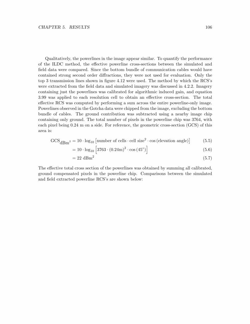
CHAPTER 5. RESULTS 106
Qualitatively, the powerlines in the image appear similar. To quantify the performanceof the ILDC method, the effective powerline cross-sections between the simulated andfield data were compared. Since the bottom bundle of communication cables would havecontained strong second order diffractions, they were not used for evaluation. Only thetop 3 transmission lines shown in figure 4.12 were used. The method by which the RCS’swere extracted from the field data and simulated imagery was discussed in 4.2.2. Imagerycontaining just the powerlines was calibrated for algorithmic induced gain, and equation3.99 was applied to each resolution cell to obtain an effective cross-section. The totaleffective RCS was computed by performing a sum across the entire powerline-only image.Powerlines observed in the Gotcha data were chipped from the image, excluding the bottombundle of cables. The ground contribution was subtracted using a nearby image chipcontaining only ground. The total number of pixels in the powerline chip was 3764, witheach pixel being 0.24 m on a side. For reference, the geometric cross-section (GCS) of thisarea is:
GCSdBm2 = 10 · log10
[number of cells · cell size2 · cos (elevation angle)
](5.5)
= 10 · log10
[3763 · (0.24m)2 · cos (45)
](5.6)
= 22 dBm2 (5.7)
The effective total cross section of the powerlines was obtained by summing all calibrated,ground compensated pixels in the powerline chip. Comparisons between the simulatedand field extracted powerline RCS’s are shown below:
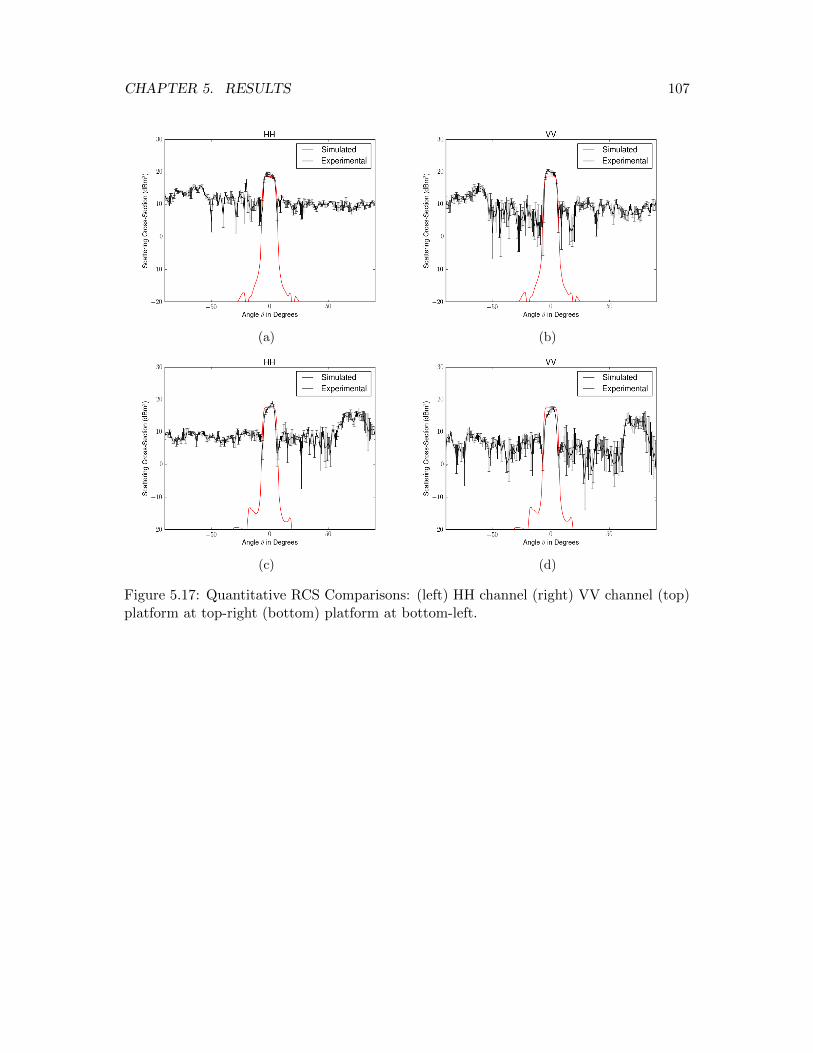
CHAPTER 5. RESULTS 107
(a) (b)
(c) (d)
Figure 5.17: Quantitative RCS Comparisons: (left) HH channel (right) VV channel (top)platform at top-right (bottom) platform at bottom-left.

CHAPTER 5. RESULTS 108
A summary of these results are provided in the table below:
Table 5.3: AFRL Gotcha results summary.
% error - % uncertainty -simulated vs. between
measured measurements
Top-right HH 0.2% 3.3%Top-right VV 3.8% 2.7%
Bottom-left HH 6.3% 3.2%Bottom-left VV 16.0% 4.1%
mean HH 3.3% 3.3%mean VV 9.9% 3.4%
mean 6.6% 3.3%
Notably, the results shown above reveal a higher amount of relative error observed whenthe platform was located in the bottom left of the image. Inspection of the field-measuredsignature in figure 5.17 shows an asymmetric sloping shape, unaccounted for in the model,and not observed for the top-right portion of the pass. Since the change in zenith anglebetween the two passes was small (less than a degree) the source of error was effected bysmall changes in optical path. This possibly points to an unaccounted for signal that mayhave resulted from coherent addition between two separate returns. It is possible, also,that second order diffraction between powerlines may have been the cause. Nominally,powerlines in separate resolution cells are incoherent with respect to each other unless asignificant amount of energy is contained in the side lobes of the impulse response. Giventhe right geometry, however, radiation which scatters off one powerline onto another andthen back to the reciever may coherently add with the first order diffraction from the latterpowerline. This could result in a signature that is very sensitive to slight asymmetry in thepowerline configuration. Imperfect knowledge of ground truth may have also been a sourceof error. The powerline configuration used for simulation was based on visual inspectionof the scene nearly a decade after the collection. It is possible that the configurationmay have changed with time. Below is an image chip of the powerlines for two differentplatform locations:
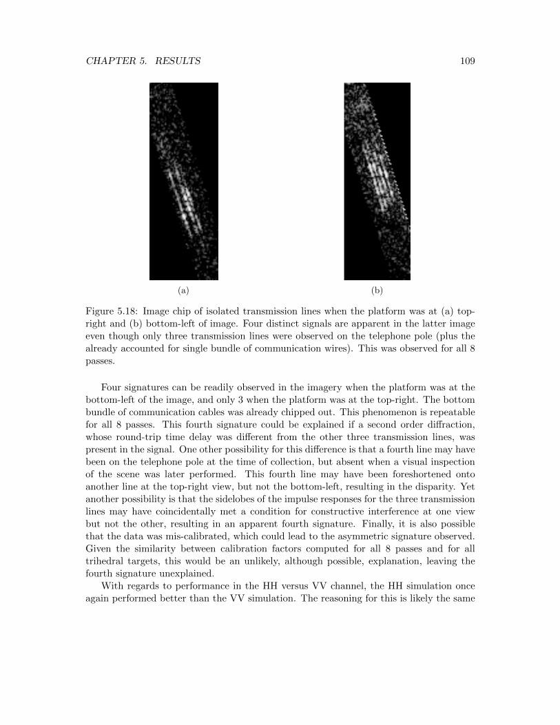
CHAPTER 5. RESULTS 109
(a) (b)
Figure 5.18: Image chip of isolated transmission lines when the platform was at (a) top-right and (b) bottom-left of image. Four distinct signals are apparent in the latter imageeven though only three transmission lines were observed on the telephone pole (plus thealready accounted for single bundle of communication wires). This was observed for all 8passes.
Four signatures can be readily observed in the imagery when the platform was at thebottom-left of the image, and only 3 when the platform was at the top-right. The bottombundle of communication cables was already chipped out. This phenomenon is repeatablefor all 8 passes. This fourth signature could be explained if a second order diffraction,whose round-trip time delay was different from the other three transmission lines, waspresent in the signal. One other possibility for this difference is that a fourth line may havebeen on the telephone pole at the time of collection, but absent when a visual inspectionof the scene was later performed. This fourth line may have been foreshortened ontoanother line at the top-right view, but not the bottom-left, resulting in the disparity. Yetanother possibility is that the sidelobes of the impulse responses for the three transmissionlines may have coincidentally met a condition for constructive interference at one viewbut not the other, resulting in an apparent fourth signature. Finally, it is also possiblethat the data was mis-calibrated, which could lead to the asymmetric signature observed.Given the similarity between calibration factors computed for all 8 passes and for alltrihedral targets, this would be an unlikely, although possible, explanation, leaving thefourth signature unexplained.
With regards to performance in the HH versus VV channel, the HH simulation onceagain performed better than the VV simulation. The reasoning for this is likely the same
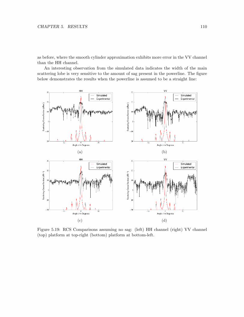
CHAPTER 5. RESULTS 110
as before, where the smooth cylinder approximation exhibits more error in the VV channelthan the HH channel.
An interesting observation from the simulated data indicates the width of the mainscattering lobe is very sensitive to the amount of sag present in the powerline. The figurebelow demonstrates the results when the powerline is assumed to be a straight line:
(a) (b)
(c) (d)
Figure 5.19: RCS Comparisons assuming no sag: (left) HH channel (right) VV channel(top) platform at top-right (bottom) platform at bottom-left.

CHAPTER 5. RESULTS 111
This finding could indicate that a method can be developed which predicts the amountof sag based on the scattering width of the main lobe. Such information would aid thosewho maintain powerlines to perform a large area assessment of which lines may be tootaught and ready to snap in the winter, or what lines are downed during a disaster.Since the amount of sag is also tied to ambient temperature, it might also be possible,given perfect knowledge of the powerline diameter and material, to gain some insight intoambient temperature based on the width of the main scattering lobe.
5.3 Summary
The baseline assessment performed for the DIRSIG simulations shows that qualitativelyrealistic imagery can be generated using this software tool in the radar modality. This isespecially valuable in the case for non-conducting distributed targets, where speckle noisedominates and specular lobe reflectance models likely suffice. For PEC targets that havea characteristic length on the order of 10’s of wavelengths or less, the lack of a physicaloptics capability leads to significant quantifiable error. This was shown to be the case inthe underestimated return for all canonical targets, the lack of sidelobes for the dihedraltargets, and the complete lack of any powerline signature in the observed imagery.
To account for the powerline return, an ILDC approach was developed. This methodproduced simulated RCS’s that exhibited an overall accuracy which fell within the uncer-tainty of data measured in a controlled environment. At X-band frequencies, the errorassociated with making the smooth cylinder approximation could be readily observed.Reasonable performance was attained at C-band, although accuracy was significantlydegraded away from normal incidence. This was likely due to the use of PTD, a high-frequency approximation technique, to model the edge contribution. The edge and endcapcontributions would probably be unobserved in actual field data.
For simulation against field data, reasonable qualitative and quantitative agreementwas attained. Errors for the effective RCS’s extracted fell within measurement uncertaintyfor the HH data but not for the VV data. This was likely due errors which arose frommaking the smooth cylinder assumption. Additionally, the shape of the RCS curves didnot match well for one of the views. This could be due to second order diffractionsbetween the closely spaced powerlines. Imperfect ground truth knowledge regarding theexact telephone pole configuration may have also induced error. The ground truth usedfor the Gotcha data was based on visual inspection of the site almost a decade after thecollection was performed.
While these results show promise and establish a foundation by which an ILDC ap-proach can be implemented for powerline modeling, additional work is needed to maturethis research. Derivation of a far-field 2D diffraction coefficient for incident TE radiation

CHAPTER 5. RESULTS 112
on a semi-open waveguide could be used to augment the smooth cylinder ILDC derived inthis research. This could improve accuracy for VV (nominally TE) polarized data. Muchwork has already been done by Sarabandi, K. and Natzke, J. [23] for variously shapedcavities whose sizes are smaller than the wavelength of the incident radiation. Field datatailored for the express purpose of extracting powerline signatures would also be beneficial.The AFRL Gotcha dataset was uniquely useful in that a full 360 view of the scene couldbe incrementally processed. Using a circular SAR collection at multiple wavelengths, withmore accurate ground truth data, would be a logical task for follow-on research. Datacollected from such an experiment could also be used to determine to what extent secondorder diffractions affect the backscattered return from a configuration of closely spacedpowerlines. Finally, it was also observed that there was a connection between the widthof the specular lobe of a powerline’s RCS and the amount of sag. If a method to extractthis information could be developed, it would be useful for surveying electrical infrastruc-ture or obtaining a rough approximation of ambient temperature when no other data isavailable.

Chapter 6
Conclusion and Future Work
There are a number of applications where a method for remotely sensing powerlines wouldbe beneficial. In the case of natural disasters, such a method could enable a wide areasurvey of the electrical infrastructure of affected locales. This survey could potentiallyshow where powerlines are down and subsequently, the areas without electricity and thecritical nodes that should be prioritized for repair. Pilots of low flying search and rescueaircraft could also incorporate this information into their mission planning.
One major obstacle to be overcome with powerline detection is collecting enough signalfor the problem to be tractable. At IR wavelengths and shorter, powerlines are often toothin and only occupy a small fraction of a pixel. At millimeter wavelengths and longer,however, powerlines become more apparent. Since powerlines are optically thin at thesewavelengths, diffraction becomes the dominant scattering mechanism.
Emperically derived matched filters for powerline detection in quad-polarization im-agery can be found in the literature [6, 46]. One way to assess the performance of thesematched filters in a cost-effective way is to model the powerline signal from first principles.This can be done for a variety of systems and orbit or flight parameters.
A number of relevant research efforts for modeling electromagnetic scattering in theradar regime were reviewed. One well known tool is GRECO [12, 13, 14, 15]. This tool usesan SBR technique with Incremental Length Diffraction Coefficients for wedges to computethe RCS of an object given a CAD model. GRECOSAR uses GRECO to build up theSAR phase history for a target. The literature provides examples for maritime applicationswhere the phase histories for individual vessels were simulated. Recent work for simulatingurban areas yielded promising results against scenes containing simple objects which couldbe easily validated. Another example found in the literature that uses a variation of theShooting and Bouncing of Rays technique is SARAS [16, 1]. This code is more focused onmodeling urban scenery. It captures many features commonly observed in SAR imagery
113

CHAPTER 6. CONCLUSION AND FUTURE WORK 114
such as Rayleigh distributed amplitude noise and downrange placement of multiple-orderreflections. One drawback to both GRECOSAR and SARAS is that they are relativelyslower than conventional, physically-based renderers that use simple ray tracing only.
For applications where radiometric accuracy is not required, a POV-RAY-based ap-proach can be found in the literature [2]. The way in which SAR images are formed createdistortions such as foreshortening and downrange placement of multiple order reflections,which are not observed in convention optical imagery. POV-RAY accounts for these fea-tures and provides geometrically accurate imagery that can increase the interpretabilityof images containing large, complex structures. Another ray-tracing based tool adaptedfor the simulation of SAR imagery is DIRSIG [7, 8]. This tool is well validated in theoptical-IR regimes and a significant amount of work has been performed for simulatingLIDAR. The radar modality of DIRSIG is relatively recent and is derived from the LIDARtoolset. Simulation of the SAR phase history is built on a pulse-by-pulse basis. For eachpulse, a bundle of rays is shot into a scene. The return signal is computed by centeringa δ-function on the time-of-flight for each ray packet, convolving the δ-functions with alinear FM signal, and then adding the contribution from all packets. Currently, only linearFM signals and simple antenna gain patterns are supported. Additionally, the scatteredamplitude is computed, using only a geometric optics approximation. This leads to anefficient method for simulating the phase history of large scenes, but the lack of an SBRcapability in the radar modality can also lead to significant errors for certain objects, aswas shown in Chapter 5, Results.
Another tool worth mentioning is Xpatch [9]. The software is proprietary but informa-tion on the website indicates it is based on an SBR approach. As was shown in this study,SBR is inadequate for modeling the return for optically thin objects such as typically sizedpowerlines at X-band frequencies and lower. In addition to general purpose radar simula-tion tools, there have also been some studies which focus on the problem of modeling howradar radiation scatters from powerlines. A notable work, led by Sarabandi, K., resultedin a MoM-based method that could be efficiently implemented at millimeter wavelengthsand shorter. Efficiency was achieved by making a physical optics approximation, whichbreaks down when the wavenumber-diameter product is . 1. This is the gap identifiedin this study, which is to derive a way of efficiently calculating the field scattered frompowerlines when the wavenumber-diameter product is . 1.
There are a variety of ways to model electromagnetic scattering depending on whatapproximations, if any, can be made for a given situation. At a top level, the RCS describeshow efficiently a target scatters incident radiation. It is a metric solely dependent on targetproperties and aspect viewing angles. The RCS does not depend on distance to the target.One way to calculate the RCS is to use equation 3.4 which relates the squared magnitudeof the incident field to the squared magnitude of the scattered far-field.

CHAPTER 6. CONCLUSION AND FUTURE WORK 115
A number of ways for calculating the scattered field were presented in Chapter 3,Theory. The discussion began with Maxwell’s equations, the solutions to which providethe most accurate results. Analytically solving these equations is only tractable whenboundary conditions can be specified in a natural coordinate system. The case of 2Dscattering from a cylinder falls into this category. In general, however, it is difficult toimpose boundary conditions for arbitrarily shaped surfaces. Numerical methods for solvingMaxwell’s equations include FDTD [21] and MoM [17]. Although these approaches provideaccurate results, stringent sampling requirements often lead to prohibitive computationtime for current commercial-off-the-shelf computing hardware.
Approximations to Maxwell’s equations are often required to calculate efficiently thescattered field. A common approximation used is geometric optics. This approach is de-rived from the 0th-order term in the Luneberg-Kline series solution to Maxwell’s equations[47]. This term leads to solutions which result in the laws of reflection and refraction, aswell expressions commonly found in radiometry. Ray tracing is often used for numericalcomputation. The geometric optics solution does not depend on frequency. It fails forlonger wavelengths, at caustics, and at sharp discontinuities such as edges or shadows. Toaccount for the scattered field from discontinuities using a geometric approach, one can usethe Geometric Theory of Diffraction (GTD) [27]. This theory provides the ray directionsthrough Fermat’s Principle for Edge Diffraction. The ray amplitudes from discontinuitiesare derived from exact canonical solutions such as Sommerfeld’s solution for scatteringfrom an infinite half plane. The GTD uses a high frequency approximation so there arelimits to its use. One notable limitation is in computing the scattered field near geometricshadow boundaries. In these regions, the GTD solution results in singularities.
Another high-frequency approximation technique commonly found in the literature isPhysical Optics (PO) [33, 47]. The term Physical Optics has various meanings dependingon the community. For radar, PO has a very specific meaning- it is the integral whichresults from making various simplifications to the integral form of Maxwell’s equations.These assumptions are: object is in the far-field; small differential regions on the surfaceare locally flat (the radius of curvature of the surface is much larger than the wavelength);and there are no source currents in the geometric shadow. This method is closely relatedto scalar diffraction theory and the Fraunhofer integral. Unlike scalar diffraction theory,however, PO retains polarization information and is not limited to two-dimensional aper-tures. In addition to breaking down when the aforementioned assumptions cannot bemade, PO also exhibits singularities in geometric shadow transition regions.
For efficiently calculating the PO integral, the Modified Equivalent Current Approxi-mation (MECA) [29] can be used. This method starts by fragmenting an object up intotriangular facets and using ray-tracing software to approximate source currents. This isdone by assuming each ray intersection represents a plane-wave incident on the surface of

CHAPTER 6. CONCLUSION AND FUTURE WORK 116
a facet, with tilt given by the incidence angle with respect to local normal. For the specificcase of triangular facets, the PO integral has an analytic form that can be efficiently cal-culated. Although PO is used to describe the scattering from perfect conductors, MECAcan be applied to di-electric materials. When multiple ray bounces are enabled and POcalculations are performed for the final bounce only, this method becomes the Shootingand Bouncing of Rays (SBR) technique [31, 32, 42].
Avoiding the singularities observed in geometric shadow transitions regions for bothGTD an PO is possible by using the Physical Theory of Diffraction (PTD) [28]. When thePO solution for scattering from an infinite half-plane is subtracted from the GTD formof Sommerfeld’s solution, the previously mentioned singularities cancel and the scatteredfield in geometric shadow transition regions evaluate to finite values. The resulting PTDsolution represents the contribution from non-uniform currents near a discontinuity, suchas an edge. PTD (as well as GTD) is often combined with SBR, where edges are identifiedas lines adjoining two adjacent facets that have surface normals whose difference exceedsome user-defined threshold. Since one-dimensional edges cannot sample a ray bundleof finite density, the facets adjoining the edge perform the sampling. Directions of theoutgoing rays are defined by Fermat’s Principle for Edge Diffraction and their amplitudesare given by the PTD diffraction coefficients. One limitation to PTD, in addition to itbeing a high-frequency technique, is that it only gives the contribution from an edge intowhat is termed the ”Keller Cone,” defined by Fermat’s Principle for Edge Diffraction. Forscattering outside the Keller Cone, Mitzner’s Incremental Length Diffraction Coefficient(ILDC) method is often used.
The approach developed in this study was based on the ILDC method first establishedby Mitzner [10]. The modeling effort started with construction of a physical model. Itwas assumed for this model that the powerline was a perfectly conducting smooth cylinderwith sag. The curve which described the amount of sag was given by a catenary. A 2Ddiffraction coefficent for forward scattering was then calculated from Maxwell’s equations.The ILDC method provided a means of extending this solution to a 3D backscatteringcoefficient. Using the definition of the RCS, a relationship between the 3D diffractioncoefficient and the powerline RCS was derived.The 3D diffraction coefficient also enabledsimulation of the powerline phase history.
Multiple validation efforts were undertaken in this study. The first effort began with anassessment of DIRSIG’s radar modality to see if that tool provided any existing capabilityfor powerline modeling. The scene used in the DIRSIG study was based off the scene inthe AFRL Gotcha collection. This scene contained a parking lot with cars, a grassy field,canonical calibration targets such as dihedrals and trihedrals, and powerlines. Materialproperties and reflectance distributions for all objects in the scene were assumed. Thereflectance distributions were based on a specular lobe model. The radar parameters and

CHAPTER 6. CONCLUSION AND FUTURE WORK 117
platform positions used in the simulation matched those extracted from the auxiliary datacontained in the Gotcha dataset. Since all parameters used in the simulation were user-defined, the simulated imagery was calibrated to units of effective RCS for each pixel.The Gotcha imagery was also calibrated using a backscatter correlation method [44] solike-to-like comparisons could be made. The features compared between the simulatedand Gotcha imagery were the amplitude noise, canonical target RCS’s, and powerlinesignatures. The amplitude noise in the DIRSIG generated image was Rayleigh distributed,as predicted by theory and observed in the Gotcha data. Qualitative scene-wide agreementwas also observed when compared to the Gotcha imagery. For the RCS’s of the canonicaltargets, significant discrepancies were noted. This was likely due to the lack of a physicaloptics capability. Finally, no powerline signal was apparent in the DIRSIG imagery. Thisdemonstrated the inability to model powerlines using a geometric optics approximation.
The other validation efforts in this study focused on assessing the efficacy of the ILDCapproach. In order to see how well RCS’s could be predicted using the relation defined byequation 3.99, measurements taken in an anechoic chamber were used. These measure-ments were obtained in a tightly controlled environment. They consisted of observationsof the scattered power for various different types of powerlines. The data was calibratedusing a standard method involving the use of a calibration sphere (section 4.2.1). Theobserved RCS’s were compared to the simulated RCS’s for validation. With few notableexceptions, the accuracy of the simulated data fell within experimental uncertainty fora variety of powerline types at both X- and C-band frequencies. Errors were somewhatlarger for the C-band measurements, especially away from normal incidence. This mayhave been due to the use of a high-frequency stationary phase technique to evaluate thescattering contribution from the endcaps. PTD coefficients for a 90 wedge were usedfor the endcap edges, and since PTD is also a high-frequency technique that does notaccount for creeping waves, the combination likely led to increased error. In both the X-and C-band frequencies, errors in the VV polarization channel were relatively higher thatthose observed in the HH polarization channel. As suggested by Sarabandi, K. et. al. [6],these errors could have resulted from making a smooth cylinder assumption for calculat-ing the 2D diffraction coefficient. This approach neglects the waveguide signature thatis stimulated when TE radiation (nominally VV) is incident upon the grooved helicallywound cables that make up a powerline.
Field measured powerline RCS’s were also extracted from the calibrated Gotcha im-agery and used for validation. These RCS’s represented a total effective RCS. In orderfor a like-to-like comparison to be made, powerline phase histories had to be simulated.This was done using equation 3.100 and information obtained from visual inspection of thescene. Once the phase histories were simulated, they were processed into images whichwere subsequently used to derive effective powerline RCS’s, measured similarly to the

CHAPTER 6. CONCLUSION AND FUTURE WORK 118
Gotcha data. The powerline phase histories were also added to the DIRSIG generatedphase history so a qualitative comparison could be made between the two sets of images.
Qualitatively, the powerline signatures observed in the simulated imagery appearedvery similar to the those in the Gotcha imagery. There was also reasonable agreementbetween the simulated and extracted RCS’s. It was also shown that the amount of sagpresent in the powerline had a significant impact on its observed signature. As with theMichigan data, greater errors were observed in the VV channel, probably for the samereason, making a smooth cylinder assumption. There was also an asymmetric slopingpattern observed in the powerlines’ RCS and an additional signal in the imagery. Theadditional signal was observed when the platform was located to the southwest. Theasymmetric sloping pattern was also more apparent when the platform was positionedto the southwest. This was observed for all 8 passes. Since the change in zenith anglebetween the two observation points was less than 1, the source of error would also havebeen susceptible to slight changes. This is possibly indicative of an unaccounted for signalresulting from two or more coherently added returns. Such a source of error could havebeen caused by second-order diffractions, or the sidelobes from all returns coincidentallylining up. An additional cable, present at the time of collection and absent when visualinspection was made, could have also led to the observed error.
The results from this study indicate that an ILDC approach to modeling the radarreturn from powerlines provides an efficient means for calculating the scattered return.The accuracy is demonstrably better than using a pure PO/PTD approach when k ·a . 1and is computationally more efficient than a MoM approach. A number of possibilitiesfor future work are opened up by this effort. For reducing the error observed in the VVchannel, a far-field 2D diffraction coefficient that takes into account the helical geometryof powerlines would increase accuracy. This diffraction coefficient could be obtained inseveral ways. For instance, a two-step analytic approach would be to derive a far-field,semi-open waveguide diffraction coefficient from a solution in the literature [23], and thenadd this as a correction term to the smooth cylinder diffraction coefficient derived inthe present research. Another numerical approach may involve using MoM to obtain thesource currents over a single period of an infinitely long powerline. A diffraction coefficientcould then be derived from the resulting far-field solution.
Another unaccounted for feature in the field data was the sloping asymmetric RCSobserved for the powerlines. Incorporating a model that accounts for 2nd-order diffractionscould improve the accuracy of the simulated data. An overall source of error for the fielddata was uncertainty in the ground truth. Future work involving a field collection morefocused on the powerline modeling problem, and with more precise ground truth, wouldalso help to mitigate any remaining sources of error.
A number of future applications can also be identified. It was shown that there was

CHAPTER 6. CONCLUSION AND FUTURE WORK 119
some relationship between the width of the main lobe in a powerline’s RCS and its sag.If such a relationship could be quantified, it could be used by maintainers of electricalinfrastructure to determine if powerlines in a certain area are in danger of snapping inwinter. Given perfect knowledge of the conducting material and tension, some measureof absolute ambient temperature, or relative ambient temperature differences from oneday to another, could be obtained from SAR imagery containing powerlines. Anotherpotential application would be in the identification of buried cables for ground-penetratingUHF/VHF SAR collections. Since there is a strong mathematical relationship between thescattering of electromagnetic radiation and acoustic waves, it may also be possible to adaptthis approach to model how underwater cables scatter an active sonar pulse. Pursuing anyof these applications can lead to an improved capability for forward modeling powerlinereturns that can then be used to evaluate a given detection algorithm for a system andscene of interest.

Bibliography
[1] G. Franceschetti, A. Iodice, D. Riccio, and G. Ruello, “SAR raw signal simulation forurban structures,” Geoscience and Remote Sensing, IEEE Transactions on, vol. 41,pp. 1986–1995, Sept 2003.
[2] S. Auer, S. Hinz, and R. Bamler, “Ray-tracing simulation techniques for understand-ing high-resolution SAR images,” Geoscience and Remote Sensing, IEEE Transac-tions on, vol. 48, pp. 1445–1456, March 2010.
[3] J. Delliere, H. Maitre, and A. Maruani, “SAR measurement simulation on urbanstructures using a FDTD technique,” in Urban Remote Sensing Joint Event, 2007,pp. 1–8, April 2007.
[4] K. Sarabandi and M. Park, “A radar cross-section model for power lines at millimeter-wave frequencies,” Antennas and Propagation, IEEE Transactions on, vol. 51, no. 9,pp. 2353–2360, 2003.
[5] Air Force Research Labs SNA, “Gotcha volumetric SAR data set overview.” https:
//www.sdms.afrl.af.mil/index.php?collection=gotcha.
[6] K. Sarabandi, Y. Oh, and F. T. Ulaby, “Polarimetric measurements of powerlinecables,” Tech. Rep. DAAH01-91-C-R066, University of Michigan, College of Engi-neering, 1991.
[7] Rochester Institute of Technology Center for Imaging Science, “DIRSIG radar modal-ity handbook.” http://www.dirsig.org/docs/new/radar.html.
[8] Rochester Institute of Technology Center for Imaging Science, “DIRSIG.” http://
www.dirsig.org/.
[9] Leidos, “Xpatch electromagnetic simulation software.” https://www.leidos.com/
products/software/xpatch.
120

BIBLIOGRAPHY 121
[10] K. Mitzner, “Incremental length diffraction coefficients,” Tech. Rep. AFAL-TR-73-296, Northrop Corporation Aircraft Division, 1974.
[11] J. Charles V. Jakowatz, D. E. Wahl, P. H. Eichel, D. C. Ghiglia, and P. A. Thompson,Spotlight-Mode Synthetic Aperture Radar: A Signal Processing Approach. Springer,1996.
[12] J. M. Ruis, M. Ferrando, and L. Jofre, “GRECO: Graphical electromagnetic com-puting for RCS prediction in real time,” IEEE Antennas and Propagation Magazine,vol. 35, pp. 7–17, April 1993.
[13] J. Mallorqui, J. Rius, and M. Bara, “Simulation of polarimetric SAR vessel signaturesfor satellite fisheries monitoring,” Geoscience and Remote Sensing Symposium, 2002.IGARSS ’02. 2002 IEEE International, vol. 5, pp. 2711–2713, 2002.
[14] G. Margarit, J. Mallorqui, J. Rius, and J. Sanz-Marcos, “On the usage ofGRECOSAR, an orbital polarimetric SAR simulator of complex targets, to vessel clas-sification studies,” Geoscience and Remote Sensing, IEEE Transactions on, vol. 44,pp. 3517–3526, Dec 2006.
[15] G. Margarit, M. J. J., and C. Lopez-Martinez, “GRECOSAR, a SAR simulator forcomplex targets: Application to urban environments,” Geoscience and Remote Sens-ing Symposium, 2007. IGARSS ’07. 2007 IEEE International, pp. 4160–4163, July2007.
[16] G. Franceschetti, M. Migliaccio, D. Riccio, and G. Schirinzi, “SARAS: a syntheticaperture radar (SAR) raw signal simulator,” Geoscience and Remote Sensing, IEEETransactions on, vol. 30, pp. 110–123, Jan 1992.
[17] R. Harington, Field Computation by Method of Moments. Hoboken, New Jersey:Wiley-IEEE Press, 1993.
[18] C. de Boor, A Practical Guide to Splines. New York: Springer-Verlag, 1978.
[19] G. Franceschetti, A. Iodice, and D. Riccio, “A canonical problem in electromagneticbackscattering from buildings,” Geoscience and Remote Sensing, IEEE Transactionson, vol. 40, pp. 1787–1801, Aug 2002.
[20] T. Griesser and C. Balanis, “Backscatter analysis of dihedral corner reflectors usingphysical optics and the physical theory of diffraction,” Antennas and Propagation,IEEE Transactions on, vol. 35, pp. 1137–1147, Oct 1987.

BIBLIOGRAPHY 122
[21] K. Yee, “Numerical solution of initial boundary value problems involving maxwell’sequations in isotropic media,” Antennas and Propagation, IEEE Transactions on,vol. 14, pp. 302–307, May 1966.
[22] K. Sarabandi, “Power lines: Radar measurements and detection algorithm for po-larimetric SAR images,” Aerospace and Electronic Systems, IEEE Transactions on,vol. 30, pp. 632–642, April 1994.
[23] T. B. Senior, K. Sarabandi, and J. R. Natzke, “Scattering by a narrow gap,” IEEEtransactions on antennas and propagation, vol. 38, no. 7, pp. 1102–1110, 1990.
[24] G. T. Ruck, Radar Cross Section Handbook. Springer, 1970.
[25] E. F. Knott, Radar Cross Section. Norwood, MA: Artech House, Inc., 2nd ed., 1993.
[26] Y. A. Kravtsov and N. Y. Zhu, “Tendencies and recent novelties in the heuristicmethods (mini-review),” in Electromagnetic Theory (EMTS), 2010 URSI Interna-tional Symposium on, pp. 974–976, IEEE, 2010.
[27] J. B. Keller, “Geometrical theory of diffraction,” Optical Society of America, vol. 52,pp. 116–130, February 1962.
[28] P. Y. Ufimtsev, Method of Edge Waves in the Physical Theory of Diffraction. Wright-Patterson AFB, OH: Foreign Technology Division, 1962.
[29] J. Meana, J. Martinez-Lorenzo, F. Las-Heras, and C. Rappaport, “Wave scatteringby dielectric and lossy materials using the modified equivalent current approximation(MECA),” IEEE Transaction on Antennas and Propogation, vol. 58, pp. 3757–3761,November 2010.
[30] J. Meana, J. Martinez-Lorenzo, and Las-Heras, “High frequency tech-niques: the physical optics approximation and the modified equiv-alent current approximation (MECA).” http://www.intechopen.com/
books/electromagnetic-waves-propagation-in-complex-matter/
high-frequency-techniques-the-physical-optics-approximation
-and-the-modified-equivalent-current-appr.
[31] H. Ling, R. C. Chou, and S. W. Lee, “Shooting and bouncing rays: Calculating theRCS of an arbitrarily shaped cavity,” IEEE Transaction on Antennas and Propoga-tion, vol. 37, pp. 194–205, February 1989.

BIBLIOGRAPHY 123
[32] H.-T. Meng, Acceleration of Asymptotic Computational Electromagnetic Physical Op-tics - Shooting and Bouncing Ray (PO-SBR) Method using CUDA. Phd, Universityof Illinois, 2011.
[33] A. Zangwill, Modern Electrodynamics. Cambridge, UK: Cambridge University Press,2013.
[34] C. A. Balanis, Advanced Engineering Electromagnetics. John Wiley & Sons, Inc.,2nd ed., 2012.
[35] S. Asano and G. Yamamoto, “Light scattering by a spheroidal particle,” Appl. Opt.,vol. 14, pp. 29–49, Jan 1975.
[36] G. B. Arfken and H. J. Weber, Mathematical Methods for Physicists. Elsevier Aca-demic Press, 6th ed., 2005.
[37] M. Born and E. Wolf, Principles of Optics. Cambridge University Press, 1999.
[38] R. G. Kouyoumjian and P. H. Pathak, “A uniform geometrical theory of diffractionfor an edge in a perfectly conducting surface,” Proceedings of the IEEE, vol. 62,pp. 1448–1461, November 1974.
[39] P. I. Ufimtsev and I. Press, Fundamentals of the physical theory of diffraction. Hobo-ken, New Jersey: Wiley, 2014.
[40] J. W. Goodman, Fourier Optics. Roberts and Company, 2005.
[41] F. Chatzigeorgiadis, Development of Code for a Physical Optics Radar Cross SectionPrediction and Analysis Application. Phd, Naval Postgraduate School, 2004.
[42] H.-J. Mametsa, F. Rouas, A. Berges, and J. Latger, “Imaging radar simulation inrealistic environment using shooting and bouncing rays technique,” in Proc. SPIE,vol. 4543, pp. 34–40, 2002.
[43] H. Goldstein, C. Poole, and J. Safko, Classical Mechanics. San Francisco, CA: Addi-son Wesley, 3rd ed., 2002.
[44] J. D. Klein, “Calibration of complex polarimetric SAR imagery using backscatter cor-relations,” Aerospace and Electronic Systems, IEEE Transactions on, vol. 28, pp. 183–193, January 1992.
[45] T. A. Warner, G. M. Foody, and M. D. Nellis, The SAGE handbook of remote sensing.Sage Publications, 2009.

BIBLIOGRAPHY 124
[46] K. Sarabandi, L. Pierce, Y. Oh, and F. T. Ulaby, “Power lines: Radar measure-ments and detection algorithm for polarimetric SAR images,” IEEE transactions onaerospace and electronic systems, vol. 30, no. 2, pp. 632–643, 1994.
[47] C. A. Balanis, Antenna Theory: Analysis and Design. John Wiley & Sons, Inc.,3rd ed., 2005.

Appendices
125
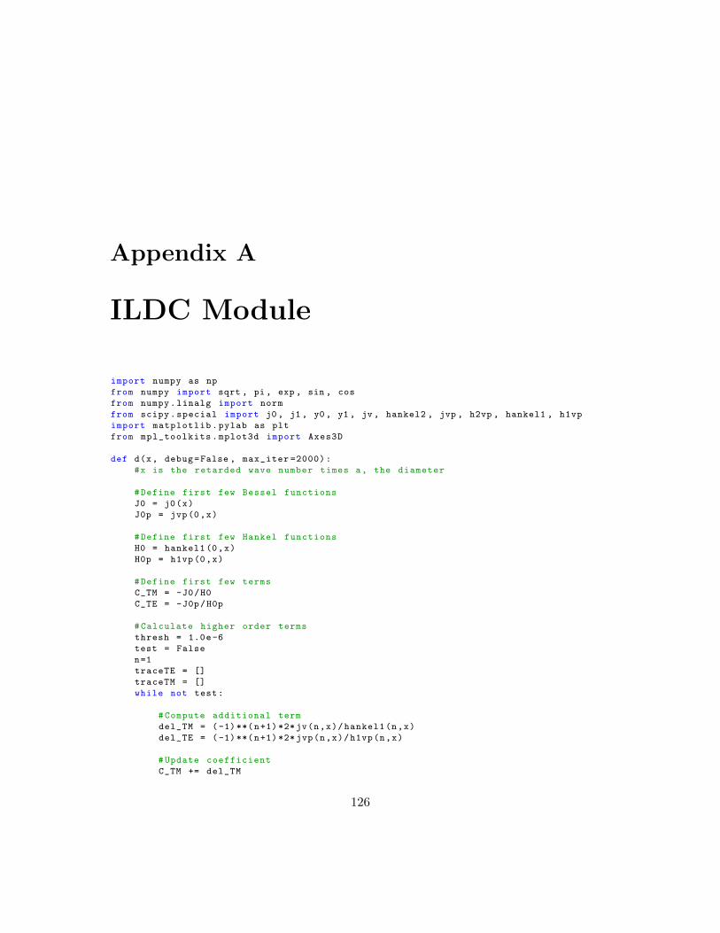
Appendix A
ILDC Module
import numpy as np
from numpy import sqrt , pi, exp , sin , cos
from numpy.linalg import norm
from scipy.special import j0, j1, y0, y1 , jv , hankel2 , jvp , h2vp , hankel1 , h1vp
import matplotlib.pylab as plt
from mpl_toolkits.mplot3d import Axes3D
def d(x, debug=False , max_iter =2000):
#x is the retarded wave number times a, the diameter
#Define first few Bessel functions
J0 = j0(x)
J0p = jvp(0,x)
#Define first few Hankel functions
H0 = hankel1(0,x)
H0p = h1vp(0,x)
#Define first few terms
C_TM = -J0/H0
C_TE = -J0p/H0p
#Calculate higher order terms
thresh = 1.0e-6
test = False
n=1
traceTE = []
traceTM = []
while not test:
#Compute additional term
del_TM = (-1)**(n+1)*2*jv(n,x)/hankel1(n,x)
del_TE = (-1)**(n+1)*2*jvp(n,x)/h1vp(n,x)
#Update coefficient
C_TM += del_TM
126

APPENDIX A. ILDC MODULE 127
C_TE += del_TE
#Perform test to see if we’ve reached the maximum nmber of iterations
#or see if the additional term is less than the threshold value
traceTM.append(abs(del_TM)/abs(C_TM))
traceTE.append(abs(del_TE)/abs(C_TE))
test1 = n>= max_iter
test2 = traceTM[n-2]. all() <=thresh
test3 = traceTE[n-2]. all() <=thresh
test = test1 | test2 | test3
#Update n
n+=1
d_TM = sqrt (2/pi)*exp(-1j*pi/4)*C_TM
d_TE = sqrt (2/pi)*exp(-1j*pi/4)*C_TE
d_out = [[d_TM ,0],[0, d_TE]]
if debug:
plt.figure ()
plt.plot(traceTE)
plt.figure ()
plt.plot(traceTM)
print(n)
return(d_out)
def D_endcap(platform , PL):
#Grab relevant parameters
a = PL[’diameter ’]/2
pos = platform[’pos’]
f_0 = platform[’f_0’]
c = 299792458.
k = 2*pi*f_0/c
rhat_i = np.zeros([len(pos) ,3])
for i in range(len(pos)):
rhat_i[i] = pos[i]/norm(pos[i],axis=-1)
nhat = -PL[’orientations ’][-1]
theta = np.pi - np.arccos(np.dot(-rhat_i , nhat))
i = np.where(theta <pi/2); theta[i] = pi-theta[i]
l = norm(PL[’r_p’][ -1])
#compute D for each point
D = [[0 ,0] ,[0 ,0]]
D[0][0] = 1j/2*a*k*np.cos(theta)/np.sin(theta)\
*j1(2*k*a*np.sin(theta))*np.exp(1j*2*k*l*np.cos(theta))
D[1][1] = -1j/2*a*k*cos(theta)/np.sin(theta)\
*j1(2*k*a*np.sin(theta))*np.exp(1j*2*k*l*np.cos(theta))
return(D)
def D_PO(platform , PL):
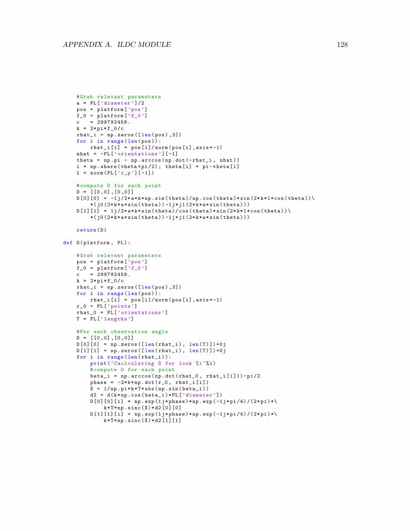
APPENDIX A. ILDC MODULE 128
#Grab relevant parameters
a = PL[’diameter ’]/2
pos = platform[’pos’]
f_0 = platform[’f_0’]
c = 299792458.
k = 2*pi*f_0/c
rhat_i = np.zeros([len(pos) ,3])
for i in range(len(pos)):
rhat_i[i] = pos[i]/norm(pos[i],axis=-1)
nhat = -PL[’orientations ’][-1]
theta = np.pi - np.arccos(np.dot(-rhat_i , nhat))
i = np.where(theta <pi/2); theta[i] = pi-theta[i]
l = norm(PL[’r_p’][ -1])
#compute D for each point
D = [[0 ,0] ,[0 ,0]]
D[0][0] = -1j/2*a*k*np.sin(theta)/np.cos(theta)*sin(2*k*l*cos(theta))\
*(j0(2*k*a*sin(theta))-1j*j1(2*k*a*sin(theta)))
D[1][1] = 1j/2*a*k*sin(theta)/cos(theta)*sin (2*k*l*cos(theta))\
*(j0(2*k*a*sin(theta))-1j*j1(2*k*a*sin(theta)))
return(D)
def D(platform , PL):
#Grab relevant parameters
pos = platform[’pos’]
f_0 = platform[’f_0’]
c = 299792458.
k = 2*pi*f_0/c
rhat_i = np.zeros([len(pos) ,3])
for i in range(len(pos)):
rhat_i[i] = pos[i]/norm(pos[i],axis=-1)
r_0 = PL[’points ’]
rhat_0 = PL[’orientations ’]
T = PL[’lengths ’]
#For each observation angle
D = [[0 ,0] ,[0 ,0]]
D[0][0] = np.zeros([len(rhat_i), len(T)])+0j
D[1][1] = np.zeros([len(rhat_i), len(T)])+0j
for i in range(len(rhat_i)):
print(’Caclculating D for look %i’%i)
#compute D for each point
beta_i = np.arccos(np.dot(rhat_0 , rhat_i[i]))-pi/2
phase = -2*k*np.dot(r_0 , rhat_i[i])
X = 1/np.pi*k*T*abs(np.sin(beta_i))
d2 = d(k*np.cos(beta_i)*PL[’diameter ’])
D[0][0][i] = np.exp(1j*phase)*np.exp(-1j*pi/4) /(2*pi)*\
k*T*np.sinc(X)*d2 [0][0]
D[1][1][i] = np.exp(1j*phase)*np.exp(-1j*pi/4) /(2*pi)*\
k*T*np.sinc(X)*d2 [1][1]

APPENDIX A. ILDC MODULE 129
D_out = ’D’ : D
PL.update(D_out)
def Efield_create(amplitude , platform):
#Get platform parameters
pos = platform[’pos’]
#Define viewing geometry
r_hat = pos/np.array([norm(pos ,axis=-1)]).T
z_hat = np.array ([0 ,0 ,1])
#Derive H and V polarization directions
H_hat = np.cross(r_hat , z_hat)/np.array ([norm(np.cross(r_hat , z_hat), axis=-1)
]).T
V_hat = np.cross(H_hat , r_hat)
E =
’H’ : amplitude*H_hat ,
’V’ : amplitude*V_hat
D_out = ’E’:E
platform.update(D_out)
def straight_PL_create(end_points , spacing , random=True , plot=False):
#Create baseline catenary that lies along the x-axis
L = norm(np.array(end_points [0])-np.array(end_points [1]))
x = np.arange(-L/2, L/2, spacing)
#Add randomness to point locations to avoid artificial interference
if random:
dx = (np.random.rand(len(x)) -0.5)*spacing
x = x+dx
#Place locations into an array
locs = np.vstack ((x, np.zeros(x.shape), np.zeros(x.shape)))
#Find how the input catenary is oriented
e = np.array(end_points [0])-np.array(end_points [1])
e_hat = e/norm(e)
theta = np.pi-np.arccos(np.dot(e_hat ,np.array ([1,0,0])))
#Rotate the baseline catenary so it is oriented with the input catenary
R_z = np.matrix ([[np.cos(theta), -np.sin(theta) ,0],
[np.sin(theta), np.cos(theta), 0],
[0,0,1]])
pos = np.matrix(locs)
pos = R_z*pos
locs = np.array(pos).T
#For two sequential points , replace with the mean value and

APPENDIX A. ILDC MODULE 130
#calculate the orientation and differential lengths
n = len(x)
locs_new = np.zeros([n-1,3])
orientations = np.zeros([n-1 ,3])
lengths = np.zeros(n-1)
for i in range(n-1):
locs_new[i] = (locs[i]+locs[i+1])/2
o = locs[i+1]-locs[i]
lengths[i] = norm(o, axis=-1)
orientations[i] = o/lengths[i]
#Translate to match input catenary
mid = (np.array(end_points [0])+np.array(end_points [1]))/2
mid[-1] = 0
locs_new = locs_new+mid
#Compute relative positions
n = len(locs_new)
r0 = locs_new[n//2]
r_p = np.zeros ([n,3])
for i in range(n):
r_p[i]=np.array(locs_new[i])-r0
#Plot catenary for diagnostic purposes
if plot:
pos = np.array(locs_new)
import matplotlib.pyplot as plt
from mpl_toolkits.mplot3d import Axes3D
fig = plt.figure ()
ax = fig.add_subplot (111, projection=’3d’)
ax.plot(pos[:,0],pos[:,1],pos[:,2])
ax.set_xlabel(’x-coordinates ’)
ax.set_ylabel(’y-coordinates ’)
ax.set_zlabel(’z-coordinates ’)
def axisEqual3D(ax):
extents = np.array([ getattr(ax, ’get_lim’.format(dim))() for dim in ’
xyz’])
sz = extents [:,1] - extents [:,0]
centers = np.mean(extents , axis =1)
maxsize = max(abs(sz))
r = maxsize /2
for ctr , dim in zip(centers , ’xyz’):
getattr(ax, ’set_lim’.format(dim))(ctr - r, ctr + r)
axisEqual3D(ax)
#Return PL dictionary
PL = ’points ’ : locs_new ,
’orientations ’: orientations ,
’lengths ’ : lengths ,
’r_p’ : r_p
return(PL)
def PL_create(end_points , sag_factor , spacing , random=True , plot=False):

APPENDIX A. ILDC MODULE 131
#Create baseline catenary that lies along the x-axis
L = norm(np.array(end_points [0])-np.array(end_points [1]))
x = np.arange(-L/2, L/2, spacing)
#Add randomness to point locations to avoid artificial interference
if random:
dx = (np.random.rand(len(x)) -0.5)*spacing
x = x+dx
#Create catenary
y = sag_factor*np.cosh(x/sag_factor)
#Get hieght of catenary to match the hieght of the input points
height_offset = end_points [0][-1]-y[0]
y = y+height_offset
#Place locations into an array
locs = np.vstack ((x, np.zeros(x.shape), y))
#Find how the input catenary is oriented
e = np.array(end_points [0])-np.array(end_points [1])
e_hat = e/norm(e)
theta = np.pi-np.arccos(np.dot(e_hat ,np.array ([1,0,0])))
#Rotate the baseline catenary so it is oriented with the input catenary
R_z = np.matrix ([[np.cos(theta), -np.sin(theta) ,0],
[np.sin(theta), np.cos(theta), 0],
[0,0,1]])
pos = np.matrix(locs)
pos = R_z*pos
locs = np.array(pos).T
#For two sequential points , replace with the mean value and
#calculate the orientation and differential lengths
n = len(x)
locs_new = np.zeros([n-1,3])
orientations = np.zeros([n-1 ,3])
lengths = np.zeros(n-1)
for i in range(n-1):
locs_new[i] = (locs[i]+locs[i+1])/2
o = locs[i+1]-locs[i]
lengths[i] = norm(o, axis=-1)
orientations[i] = o/lengths[i]
#Translate to match input catenary
mid = (np.array(end_points [0])+np.array(end_points [1]))/2
mid[-1] = 0
locs_new = locs_new+mid
#Compute relative positions
n = len(locs_new)
r0 = locs_new[n//2]
r_p = np.zeros ([n,3])
for i in range(n):

APPENDIX A. ILDC MODULE 132
r_p[i]=np.array(locs_new[i])-r0
#Plot catenary for diagnostic purposes
if plot:
pos = np.array(locs_new)
fig = plt.figure ()
ax = fig.add_subplot (111, projection=’3d’)
ax.plot(pos[:,0],pos[:,1],pos[:,2])
ax.set_xlabel(’x-coordinates ’)
ax.set_ylabel(’y-coordinates ’)
ax.set_zlabel(’z-coordinates ’)
def axisEqual3D(ax):
extents = np.array([ getattr(ax, ’get_lim’.format(dim))() for dim in ’
xyz’])
sz = extents [:,1] - extents [:,0]
centers = np.mean(extents , axis =1)
maxsize = max(abs(sz))
r = maxsize /2
for ctr , dim in zip(centers , ’xyz’):
getattr(ax, ’set_lim’.format(dim))(ctr - r, ctr + r)
axisEqual3D(ax)
#Return PL dictionary
PL = ’points ’ : locs_new ,
’orientations ’: orientations ,
’lengths ’ : lengths ,
’r_p’ : r_p
return(PL)
def PL_append (*argv , plot=True):
if plot:
fig = plt.figure ()
ax = fig.add_subplot (111, projection=’3d’)
i = 0
for PL in argv:
if i == 0:
PL_out = dict(PL)
PL_out[’diameter ’] = np.ones(len(PL[’points ’]))*PL[’diameter ’]
else:
PL_out[’orientations ’] = np.vstack (( PL_out[’orientations ’], PL[’
orientations ’]))
PL_out[’r_p’] = np.vstack (( PL_out[’r_p’], PL[’r_p’]))
PL_out[’points ’] = np.vstack (( PL_out[’points ’], PL[’points ’]))
PL_out[’lengths ’] = np.hstack (( PL_out[’lengths ’], PL[’lengths ’]))
PL_out[’diameter ’] = np.append(PL_out[’diameter ’],
np.ones(len(PL[’points ’]))*PL[’diameter ’]
)
i+=1
#Plot catenary for diagnostic purposes
if plot:

APPENDIX A. ILDC MODULE 133
pos = np.array(PL[’points ’])
ax.plot(pos[:,0],pos[:,1],pos[:,2])
ax.set_xlabel(’x-coordinates ’)
ax.set_ylabel(’y-coordinates ’)
ax.set_zlabel(’z-coordinates ’)
def axisEqual3D(ax):
extents = np.array([ getattr(ax, ’get_lim’.format(dim))() for dim
in ’xyz’])
sz = extents [:,1] - extents [:,0]
centers = np.mean(extents , axis =1)
maxsize = max(abs(sz))
r = maxsize /2
for ctr , dim in zip(centers , ’xyz’):
getattr(ax, ’set_lim’.format(dim))(ctr - r, ctr + r)
axisEqual3D(ax)
return(PL_out)
def D_HV(platform , PL):
#Calculate 3D diffraction coefficient using platform
#polarization vectors
f_0 = platform[’f_0’]
c = 299792458.
k = 2*pi*f_0/c
views = len(platform[’pos’])
T = PL[’lengths ’]
#Calculate basis vectors
t_hat = PL[’orientations ’]
z_hat = np.array ([0 ,0 ,1])
r_hat = -platform[’pos’]/np.array([norm(platform[’pos’], axis=-1)]).T
#H = platform[’E ’][’H’]
#V = platform[’E ’][’V’]
H = np.cross(r_hat , z_hat)/np.array([norm(np.cross(r_hat , z_hat), axis=-1)]).T
V = np.cross(H, r_hat)
#Initialize D
D = [[0 ,0] ,[0 ,0]]
D[0][0] = np.zeros([len(r_hat), len(T)])+0j
D[0][1] = np.zeros([len(r_hat), len(T)])+0j
D[1][0] = np.zeros([len(r_hat), len(T)])+0j
D[1][1] = np.zeros([len(r_hat), len(T)])+0j
for i in range(views):
print(’Calculating D_II for view %i’%i)
#Calculate D for each point , for each look
beta_i = np.arccos(np.dot(t_hat , r_hat[i]))-pi/2
X = 1/np.pi*k*T*abs(np.sin(beta_i))
d2 = d(k*np.cos(beta_i)*PL[’diameter ’])
DTM = np.exp(-1j*pi/4) /(2*pi)*k*T*np.sinc(X)*d2 [0][0] #
DTE = np.exp(-1j*pi/4) /(2*pi)*k*T*np.sinc(X)*d2 [1][1] #

APPENDIX A. ILDC MODULE 134
#Calculate basis vectors for each point
TE = np.cross(t_hat , r_hat[i]); TE = TE/np.array ([norm(TE , axis=-1)]).T
TM = np.cross(r_hat[i], TE)
TEs = 1*TE
TMs = -1*TM
#Calculate II for each point
D[0][0][i] = DTM*abs(np.dot(TM, H[i])*np.dot(TMs , H[i]))+\
DTE*abs(np.dot(TE, H[i])*np.dot(TEs , H[i]))
D[0][1][i] = DTM*abs(np.dot(TM, H[i])*np.dot(TMs , V[i]))+\
DTE*abs(np.dot(TE, H[i])*np.dot(TEs , V[i]))
D[1][0][i] = DTM*abs(np.dot(TM, V[i])*np.dot(TMs , H[i]))+\
DTE*abs(np.dot(TE, V[i])*np.dot(TEs , H[i]))
D[1][1][i] = DTM*abs(np.dot(TM, V[i])*np.dot(TMs , V[i]))+\
DTE*abs(np.dot(TE, V[i])*np.dot(TEs , V[i]))
D_out = ’D_HV’: D
PL.update(D_out)
def RECT(t,T):
f = np.zeros(len(t))
f[(t/T <0.5) & (t/T >-0.5)] = 1
return f
def simulate_PL_phs(platform , PL, amplitude =1):
#Retrieve relevent parameters
c = 299792458.
gamma = platform[’chirprate ’]
f_0 = platform[’f_0’]
t = platform[’t’]
pos = platform[’pos’]
views = len(platform[’pos’])
nsamples= platform[’nsamples ’]
T_p = platform[’T_p’]
D_HV = PL[’D_HV’]#PL[’D’] #
points = PL[’points ’]
#Simulate the phase history for each pulse , for each point
phs = np.zeros ([4,views , nsamples ])+0j
for i in range(views):
print(’simulating pulse %i’%(i+1))
R_0 = norm(pos[i])
j=0
for p in points:
R_t = norm(pos[i]-p)
dr = R_t -R_0
phase = pi*gamma *(2*dr/c)**2-\
2*pi*(f_0+gamma*t)*2*dr/c
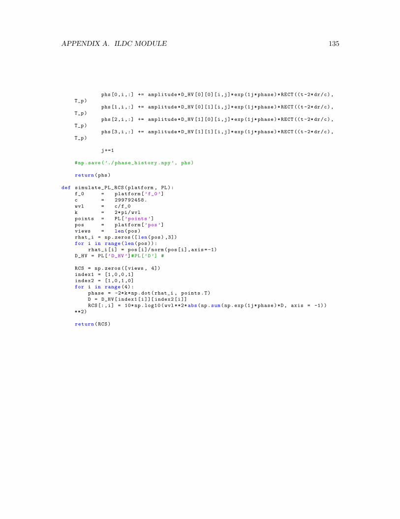
APPENDIX A. ILDC MODULE 135
phs[0,i,:] += amplitude*D_HV [0][0][i,j]*exp(1j*phase)*RECT((t-2*dr/c),
T_p)
phs[1,i,:] += amplitude*D_HV [0][1][i,j]*exp(1j*phase)*RECT((t-2*dr/c),
T_p)
phs[2,i,:] += amplitude*D_HV [1][0][i,j]*exp(1j*phase)*RECT((t-2*dr/c),
T_p)
phs[3,i,:] += amplitude*D_HV [1][1][i,j]*exp(1j*phase)*RECT((t-2*dr/c),
T_p)
j+=1
#np.save(’./ phase_history.npy ’, phs)
return(phs)
def simulate_PL_RCS(platform , PL):
f_0 = platform[’f_0’]
c = 299792458.
wvl = c/f_0
k = 2*pi/wvl
points = PL[’points ’]
pos = platform[’pos’]
views = len(pos)
rhat_i = np.zeros([len(pos) ,3])
for i in range(len(pos)):
rhat_i[i] = pos[i]/norm(pos[i],axis=-1)
D_HV = PL[’D_HV’]#PL[’D ’] #
RCS = np.zeros ([views , 4])
index1 = [1,0,0,1]
index2 = [1,0,1,0]
for i in range (4):
phase = -2*k*np.dot(rhat_i , points.T)
D = D_HV[index1[i]][ index2[i]]
RCS[:,i] = 10*np.log10(wvl **2* abs(np.sum(np.exp(1j*phase)*D, axis = -1))
**2)
return(RCS)

Appendix B
RCS Simulation Code
#if __name__ == ’__main__ ’:
#Add include directories to default path list
from sys import path
from numpy import *
from matplotlib.pylab import *
path.append(’../’)
import re
import numpy as np
from numpy import *
import matplotlib
import matplotlib.lines as mlines
from matplotlib import rc
rc(’text’, usetex=True)
rc(’font’, size =14)
import warnings
warnings.filterwarnings(’ignore ’, category=RuntimeWarning)
from functions import *
from PTD_functions import *
end_points1 = ([0, 0.3048/2 , 0], [0, -0.3048/2 , 0])
#end_points1 = ([0, 3*wvl/2, 0], [0, -3*wvl/2, 0])
#end_points1 = ([0, 40/2, 0], [0, -40/2, 0])
obj = ’cyl1’
#Import Experimental RCS
###########################################################################
fname = "../ Experimental RCS data/xband/1ft_"+obj+"_msav"
#fname = "../ Experimental RCS data/cband /"+obj+"_msav"
f = open(fname , ’r’)
r = re.compile(’ -?\d+\.\d+’)
RCS = []
for line in f:
m = r.findall(line)
if m != []:
136

APPENDIX B. RCS SIMULATION CODE 137
RCS.append(m)
f.close()
#fname = "../ Experimental RCS data/cband /"+obj+"_mser.npy"
fname = "../ Experimental RCS data/xband/1ft_"+obj+"_mser.npy"
RCS_err = np.load(fname)
#Define Simulation Parameters
###########################################################################
diameter = 0.0127#3*wvl #wvl #
a = diameter /2
f_0 = 9.5e9
#f_0 = 4.75e9
RCS = np.array(RCS , dtype = float64)
#theta = linspace(0, 90, 2000)*pi/180
#theta = linspace(RCS [: ,0].min(), RCS[:,0]. max(), 150)*pi/180
theta = (RCS [: ,0]+0)*pi/180
#Create/Import Platform Dictionary
###########################################################################
r0 = matrix ([[-1,0,0]]).T#*1/ sqrt (2)
n = len(theta)
p = zeros([n,3])
for i in range(n):
R = matrix ([
[cos(theta[i]), -sin(theta[i]), 0],
[sin(theta[i]), cos(theta[i]), 0],
[0, 0, 1]
])
p[i] = squeeze(R*r0)
platform = ’pos’ : p
platform[’f_0’] = f_0
#Create Power Line Object
###########################################################################
n_runs = 5
sigmaHH = 0
sigmaVV = 0
for i in range(n_runs):
print(’run %i’%(i+1))
PL = straight_PL_create(end_points1 , spacing = 0.01, random=False)
#PL = PL_create(end_points1 , sag_factor = -1, spacing = 0.01, random=True , plot
=False)
PL[’diameter ’] = diameter
#Compute Endcap Contribution
###########################################################################
D_end = D_endcap(platform , PL)#[[0 ,0] ,[0 ,0]]#
#Compute Edge Contribution
###########################################################################

APPENDIX B. RCS SIMULATION CODE 138
D_edge = D_edge_HF(platform , PL)#, npoints = 10000)
#D_edge = D_edge_exact(platform , PL, npoints =1000)
i = np.where(theta ==0)
D_edge [0][0][i]= D_edge [0][0][i[0]+1]; D_edge [1][1][i]= D_edge [1][1][i[0]+1]
D_end [0][0] += D_edge [0][0]
D_end [1][1] += D_edge [1][1]
#Update PL Object with D Values
###########################################################################
D_HV(platform , PL)
#Compute 3D RCS
###########################################################################
D3 = PL[’D_HV’]
#D3 = D_PO(platform , PL)
#D3 = [[0 ,0] ,[0 ,0]]
c = 299792458
wvl = c/f_0
k = 2*pi/wvl
sigma_d = pi*a**2*(k*a)**2
sigmaHH += wvl **2* abs(sum(D3[0][0] , axis=-1)+D_end [0][0]) **2
sigmaVV += wvl **2* abs(sum(D3[1][1] , axis=-1)+D_end [1][1]) **2
#sigmaHH += wvl **2* abs(D3 [0][0]+ D_end [0][0]) **2
#sigmaVV += wvl **2* abs(D3 [1][1]+ D_end [1][1]) **2
#sigmaHH_PO =0; sigmaVV_PO =0
#sigmaHH_PO += wvl **2* abs(D3 [0][0]+ D_end [0][0] - D_edge [0][0]) **2
#sigmaVV_PO += wvl **2* abs(D3 [1][1]+ D_end [1][1] - D_edge [1][1]) **2
#sigmaHH_end =0; sigmaVV_end =0
#sigmaHH_end += wvl **2* abs(D_edge [0][0]) **2
#sigmaVV_end += wvl **2* abs(D_edge [1][1]) **2
sigmaHH = sigmaHH/n_runs
sigmaVV = sigmaVV/n_runs
sigmaHH_err = 10* log10 (1+wvl **2* sin(theta)/((k*a)**2* sigmaHH))
sigmaVV_err = 10* log10 (1+wvl **2* sin(theta)/((k*a)**2* sigmaVV))
#Comparison Plots
###########################################################################
figure ()
#title(’VV RCS Using PO/PTD ’)
title(’VV RCS Using Exact ILDC Plus PO/PTD Endcaps ’)
plot(theta *180/pi , 10* log10(sigmaVV), color=’red’)
plot(theta *180/pi , 10* log10(sigmaVV)+sigmaVV_err /2, linestyle=’--’, color=’red’)
plot(theta *180/pi , 10* log10(sigmaVV)-sigmaVV_err /2, linestyle=’--’, color=’red’)
errorbar(RCS[:,0], RCS[:,1], yerr=RCS_err [:,1], color=’black’)
#plot(RCS[:,0], RCS[:,1], color=’black ’)
ylim ([ -60 ,10])
ylabel(’Scattering Cross -Section (dBm$^2$)’)

APPENDIX B. RCS SIMULATION CODE 139
xlabel(’Angle $\\ vartheta$ in Degrees ’)
simulated = mlines.Line2D ([], [], color=’red’, linestyle=’-’, label=’Simulated ’)
experimental = mlines.Line2D ([], [], color=’black’, linestyle=’-’, label=’
Experimental ’)
plt.legend(handles =[simulated , experimental ])
#title(’VV d=$\lambda$ , L=3$\lambda$ ’)
#plot(theta *180/pi+90, 10* log10(sigmaVV /( sigma_d*pi)), color=’black ’)
#plot(theta *180/pi+90, 10* log10(sigmaVV_PO /( sigma_d*pi)), linestyle=’--’, color=’
black ’)
#plot(theta *180/pi+90, 10* log10(sigmaVV_end /( sigma_d*pi)), linestyle=’:’, color=’
black ’, linewidth =2)
#legend([’PTD VV’, ’PO’, ’Nonuniform / Fringe Component ’])
#ylim ([ -40 ,20])
#ylabel(’Normalized Scattering Cross -Section ’)
#xlabel(’Angle $\\ vartheta$ in Degrees ’)
figure ()
#title(’HH RCS Using PO/PTD ’)
title(’HH RCS Using Exact ILDC Plus PO/PTD Endcaps ’)
plot(theta *180/pi , 10* log10(sigmaHH), color=’red’)
plot(theta *180/pi , 10* log10(sigmaHH)+sigmaHH_err /2, linestyle=’--’, color=’red’)
plot(theta *180/pi , 10* log10(sigmaHH)-sigmaHH_err /2, linestyle=’--’, color=’red’)
errorbar(RCS[:,0], RCS[:,2], yerr=RCS_err [:,2], color=’black’)
#plot(RCS[:,0], RCS[:,2], color=’black ’)
ylim ([ -60 ,10])
ylabel(’Scattering Cross -Section (dBm$^2$)’)
xlabel(’Angle $\\ vartheta$ in Degrees ’)
simulated = mlines.Line2D ([], [], color=’red’, linestyle=’-’, label=’Simulated ’)
experimental = mlines.Line2D ([], [], color=’black’, linestyle=’-’, label=’
Experimental ’)
plt.legend(handles =[simulated , experimental ])
#title(’HH d=$\lambda$ , L=3$\lambda$ ’)
#plot(theta *180/pi+90, 10* log10(sigmaHH /( sigma_d*pi)), linestyle=’--’, color=’black
’)
#plot(theta *180/pi+90, 10* log10(sigmaHH_PO /( sigma_d*pi)), color=’black ’)
#plot(theta *180/pi+90, 10* log10(sigmaHH_end /( sigma_d*pi)), linestyle=’:’, color=’
black ’, linewidth =2)
#legend([’PTD HH’, ’PO’, ’Nonuniform / Fringe Component ’])
#ylim ([ -40 ,20])
#ylabel(’Normalized Scattering Cross -Section ’)
#xlabel(’Angle $\\ vartheta$ in Degrees ’)
’’’
figure ()
plot(log10(abs(D_edge [0][0]) **2))
plot(log10(abs(D_edge2 [0][0]) **2))
figure ()
plot(log10(abs(D_edge [1][1]) **2))
plot(log10(abs(D_edge2 [1][1]) **2))
’’’

Appendix C
Phase History Simulation Code
#Include standard library dependencies
import numpy as np
from matplotlib import cm
cmap = cm.Greys_r
import cv2
#Include SARIT toolset
from ritsar import phsRead
from ritsar import imgTools
from ritsar import phsTools
from sys import path
path.append(’../’)
#Create PL PHS
###############################################################################
from functions import *
off_l = 1.1
imb = 1
diameter = 0.0222
end_points1 = ([-48.3, 31.4, 13], [-1.2, 48.9, 13])
r = array(end_points1 [1])-array(end_points1 [0]); r = r/norm(r)
off = cross(r,array ([0,0,1]))*off_l
off_l = 2* off_l
end_points2 = ([-48.3-off[0], 31.4-off[1], 13-off_l], [-1.2-off[0], 48.9-off[1],
13-imb*off_l ])
end_points3 = ([ -48.3+ off[0], 31.4+ off[1], 13-off_l], [ -1.2+ off[0], 48.9+ off[1],
13-imb*off_l ])
end_points4 = ([-48.3, 31.4, 6.5], [-1.2, 48.9, 6.5])
#Create Power Line Object
###########################################################################
PL1 = PL_create(end_points1 , sag_factor = 250, spacing = 0.1, random=False , plot=
False)
140
APPENDIX C. PHASE HISTORY SIMULATION CODE 141
PL1[’diameter ’] = diameter
PL2 = PL_create(end_points2 , sag_factor = 250, spacing = 0.1, random=False , plot=
False)
PL2[’diameter ’] = diameter
PL3 = PL_create(end_points3 , sag_factor = 250, spacing = 0.1, random=False , plot=
False)
PL3[’diameter ’] = diameter
PL4 = PL_create(end_points4 , sag_factor = 350, spacing = 0.1, random=False , plot=
False)
PL4[’diameter ’] = diameter
PL = PL_append(PL1 , PL2 , PL3 , PL4 , plot=True)#PL4 , plot=False)#
#Include SARIT toolset
from ritsar import phsTools
from ritsar import imgTools
from ritsar import phsRead
#Create platform dictionary
import pickle
platform = pickle.load(open(’./ platforms/sim_AFRL_high_sampling ’, ’rb’))
#Create image plane dictionary
img_plane = imgTools.img_plane_dict(platform , res_factor =1.4, aspect = 1)
#Simulate phase history
wvl = 299792458./ platform[’f_0’]
R0 = norm(platform[’pos’][0])
#Efield_create(sqrt(P/(4*pi*R0**2)),platform)
D_HV(platform , PL)
phs_PL = simulate_PL_phs(platform , PL)
#Apply RVP correction
for i in range (4):
phs_PL[i] = phsTools.RVP_correct(phs_PL[i], platform)
np.save(’./ phase_histories /% sPL_phs ’%diameter , phs_PL)
#Import DIRSIG PHS
###############################################################################
#Define directory containing *.au2 and *.phs files
directory = ’./ DIRSIG_data/full_ap1/’
#Import phase history and create platform dictionary
[phs_DIRS , platform] = phsRead.DIRSIG(directory)
#Add two phase histories
phs = phs_PL
platform_sub = dict(platform)
ppd = len(platform[’pos’])/360
dpi = 3
img = np.zeros ([4, 360-dpi ,512 ,512]) +0j
pol = [’HH’, ’HV’, ’VH’, ’VV’]
for i in [0 ,3]:

APPENDIX C. PHASE HISTORY SIMULATION CODE 142
img_number = 0
for j in range (0,360-dpi):
pulse0 = int(j*ppd)
pulse1 = int((j+dpi)*ppd -1)
pulse_index = np.arange(pulse0 , pulse1)
phs_sub = phs[i, pulse_index ,:]
npulses = int(phs_sub.shape [0])
platform_sub[’npulses ’] = npulses
platform_sub[’pos’] = platform[’pos’][ pulse_index]
if i == 0:
img_plane = imgTools.img_plane_dict(platform_sub , res_factor =1.4,
aspect =1.0, upsample=True)
img[i, img_number , :, :] = imgTools.backprojection(phs_sub , platform_sub ,
img_plane)
img_number +=1
np.save(’./imgs/%sPL’%diameter ,img)
t = platform[’t’]
T_p = t.max()-t.min()
adv = len(img[i])*3//4
img2 = np.roll(img , adv , axis =1)
img2 = img2.T/69373421.298985541
#Make RCS
RCS = 10* log10(wvl **2* sum(abs(img2)**2, axis =(0,1)))
np.save(’./RCSs/% sPL_RCS ’%diameter ,RCS)
#Create video writer
for i in [0 ,3]:
fname = ’./ videos /%sPL_%s.avi’%(diameter , pol[i])
fourcc = cv2.VideoWriter_fourcc(’I’,’Y’,’U’,’V’)
fps = 20
size = (512 ,512)
frame = 10*np.log10(abs(img2[:,:,:,i])/(abs(img2[:,:,:,i]).max()))
writer = cv2.VideoWriter(fname , fourcc , fps , size)
for j in range (360-dpi):
frame_i = frame [::-1,:,j]#frame[::-1,:,i]
frame_i[frame_i <-35]=-35
frame_i = frame_i -frame_i.min()
frame_i = frame_i/frame_i.max()
writer.write(frame_i)
print(j)
writer.release ()