Modelling and Optimization of Compact subseaseparators

Fahad Matovu

Supervisor: Johannes JaschkeCo-Supervisor: Sigurd Skogestad

NTNU

June 3, 2015

1 / 17

Outline

IntroductionMotivationModelling of Separation unitsOptimization of systemResultsConclusionReferences

2 / 17

Introduction

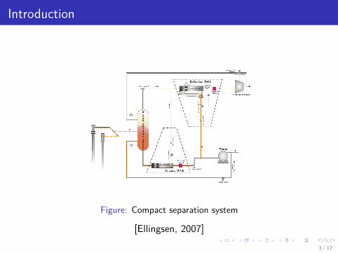
Figure: Compact separation system

[Ellingsen, 2007]

3 / 17

Introduction

Compact systems-minimise space and weight while optimizingseparation efficiencies.“Inline” technology-designed to have almost the same dimensions asthe transport pipe.Use centrifugal forces thousands of times greater than gravitationalforces used in conventional separators [Hamoud et.al, 2009].

Motivation;

Application in existing installations makes increased productionpossible [FMCtechnologies, 2011].Reduced size and weight limits on space and load requirements thusreducing on associated costs.Applicable top-side and sub-sea due to small size.

4 / 17

Modelling of separation units

Aim: Predict phase separation and outlet flow rates and fractions based onknown inlet conditions and separator geometry.

Gravity separatorInlet pipe entrainmentDroplet size distribution (Upper-limit log normaldistribution)[Simmons M.J., Hanratty T.J., 2001]Determine “critical” droplet size for separation

DeliquidizerUniform droplet distributionRadial settling velocityTime of flight modelSeparation efficiency

Degasser-concepts similar to deliquidizer.

5 / 17

Optimization of the system

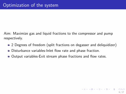
Aim: Maximize gas and liquid fractions to the compressor and pumprespectively.

2 Degrees of freedom (split fractions on degasser and deliquidizer)Disturbance variables-Inlet flow rate and phase fraction.Output variables-Exit stream phase fractions and flow rates.

6 / 17

Optimization of the system

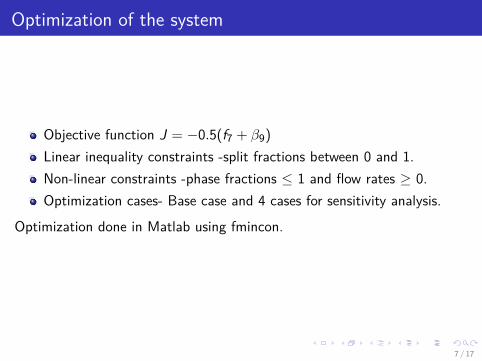
Objective function J = −0.5(f7 + β9)Linear inequality constraints -split fractions between 0 and 1.Non-linear constraints -phase fractions ≤ 1 and flow rates ≥ 0.Optimization cases- Base case and 4 cases for sensitivity analysis.

Optimization done in Matlab using fmincon.

7 / 17

Results-Gravity separator

0 50 100 150 200 2500

20

40

60

80

100

Inlet flow rate q in m3/h

Sep

eff.

liquid

Plot of Sep.eff. liquid

f=0.7f=0.5

0 50 100 150 200 2500

20

40

60

80

100

Inlet flow rate q in m3/h

Sep

.eff

gas

Plot of Sep.eff. gas

f=0.7f=0.5

0 50 100 150 200 2500

0.2

0.4

0.6

0.8

1

Inlet flow rate q in m3/h

Liq

.vol

frac

tion

Plot of Liqud vol fraction bottom stream

f=0.7f=0.5

0 50 100 150 200 2500

0.2

0.4

0.6

0.8

1

Inlet flow rate q in m3/h

gas

.vol

frac

tion

Plot of gas vol fraction top stream

f=0.7f=0.5

8 / 17

Results-Gravity separator

ExplanationLow q, low gas velocity ug, high terminal velocity ut, high liq sep.eff↑ q, ↑ ug > ut, liq in gas and ↓ Gas vol fraction GVF.For gas, smaller rise velocity ur(high liq viscosity), high bottom liqvelocity ul, gas in liq bottom stream, ↓ LVF bottom stream.Sep. eff drop more pronounced in gas. Gas low ur(high liq viscosity),liq high ut(low gas viscosity).Same q, ↓ inlet gas fraction f(0.7 to 0.5), ↑ gas entrainment, ↓ gas.sep eff. Bottom more gas thus ↓ in LVF and top less gas ↓ in GVF.

9 / 17

Results-Deliquidizer

0 50 100 150 2000

2

4

6

8

10

Inlet flow rate q in m3/h

Angu

lar

velo

city

Plot of angular velocity

F=0.85F=0.7

0 50 100 150 2000

0.2

0.4

0.6

0.8

1

Inlet flow rate q in m3/h

Effi

cien

cy

Plot of sep. efficiency

F=0.85F=0.7

0 50 100 150 2000

0.2

0.4

0.6

0.8

1

Inlet flow rate q in m3/h

LV

F

Plot of Liquid vol. fraction bottom stream

F=0.85F=0.7

0 50 100 150 2000.5

0.6

0.7

0.8

0.9

1

Inlet flow rate q in m3/h

GV

F

Plot of gas.vol fraction top stream

F=0.85F=0.7

Expt. data

10 / 17

Results-Deliquidizer

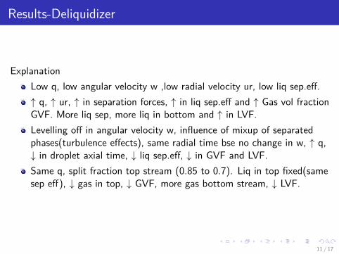
ExplanationLow q, low angular velocity w ,low radial velocity ur, low liq sep.eff.↑ q, ↑ ur, ↑ in separation forces, ↑ in liq sep.eff and ↑ Gas vol fractionGVF. More liq sep, more liq in bottom and ↑ in LVF.Levelling off in angular velocity w, influence of mixup of separatedphases(turbulence effects), same radial time bse no change in w, ↑ q,↓ in droplet axial time, ↓ liq sep.eff, ↓ in GVF and LVF.Same q, split fraction top stream (0.85 to 0.7). Liq in top fixed(samesep eff), ↓ gas in top, ↓ GVF, more gas bottom stream, ↓ LVF.

11 / 17

Results-Degasser

0 50 100 150 2000

2

4

6

8

10

Inlet flow rate q in m3/h

Angu

lar

velo

city

Plot of angular velocity

F=0.2F=0.4

0 50 100 150 2000

0.2

0.4

0.6

0.8

1

Inlet flow rate q in m3/h

Effi

cien

cy

Plot of sep. efficiency

F=0.2F=0.4

0 50 100 150 2000

0.2

0.4

0.6

0.8

1

Inlet flow rate q in m3/h

LV

F

Plot of Liquid vol. fraction bottom stream

F=0.2F=0.4

0 50 100 150 2000

0.2

0.4

0.6

0.8

1

Inlet flow rate q in m3/h

GV

F

Plot of gas.vol fraction top stream

F=0.2F=0.4

12 / 17

Results-Degasser

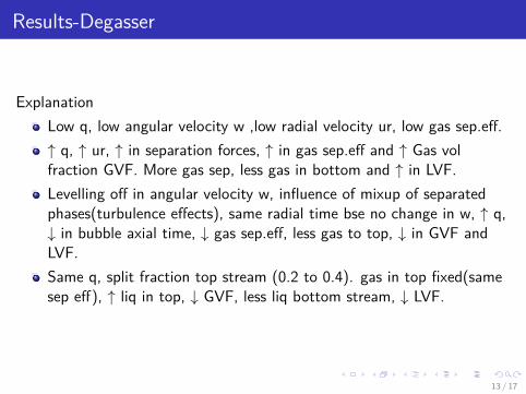
ExplanationLow q, low angular velocity w ,low radial velocity ur, low gas sep.eff.↑ q, ↑ ur, ↑ in separation forces, ↑ in gas sep.eff and ↑ Gas volfraction GVF. More gas sep, less gas in bottom and ↑ in LVF.Levelling off in angular velocity w, influence of mixup of separatedphases(turbulence effects), same radial time bse no change in w, ↑ q,↓ in bubble axial time, ↓ gas sep.eff, less gas to top, ↓ in GVF andLVF.Same q, split fraction top stream (0.2 to 0.4). gas in top fixed(samesep eff), ↑ liq in top, ↓ GVF, less liq bottom stream, ↓ LVF.

13 / 17

Optimization results

Table: Optimization results for the 5 different cases

Case2(+5% q1), Case3(−5% q1), Case4(+10% f1) and Case5(−10% f1)Variable Init. guess Base-case Case2 Case3 Case4 Case5

F1 0.2 0.3384 0.3898 0.2658 0.1327 0.3788F2 0.6 0.9951 0.9939 0.9962 0.9937 0.9964J - 0.9748 0.9917 0.9483 0.8953 0.9877

Optimal performance indicates no liquid in top stream from degasser andno gas in bottom stream from deliquidizer.An average of not more that 5% of undesirable phase in exit streams tothe compressor and pump.

14 / 17

Sensitivity analysis

Relative sensivity SCP = ∂Copt/Copt

∂P/P [Edgar et.al, 1989].

Table: Sensitivity analysis

Cases SJq1 SF1

q1 SF2q1 SJ

α1 SF1α1 SF2

α1Case2 0.35 3.04 -0.02 - - -Case3 0.54 4.29 -0.02 - - -Case4 - - - -0.82 -6.08 -0.01Case5 - - - -0.13 -1.19 -0.01

Largest relative influence on optimal F1 by changes in q1 and α1

15 / 17

Conclusion

Steady state models have been developed for predicting phaseseparation of gas and liquid phases and trends in results are inagreement with theoretical expectations.Optimization has been carried out. Results have shown an average ofnot more that 5% of dispersed phase in continuous phase in exitstreams to the compressor and pump.

ShortcomingsLack of experimental data.

16 / 17

References

Christian Ellingsen (2007)Compact sub sea separation: Implementation and comparison of two differentcontrol structuresMaster Thesis, NTNU

A Hamoud(2009)New application of an inline separation technology in a real wet gas field.Saudi Aramco Journal of Technology.

FMCtechnologies (2011)Compact total separation systems.

M.J.,Simmons,T.J.,Hanratty(2001)Droplet size measurements in horizontal annular gas-liquid flow.International Journal of Multiphase flow 27 (5), 861–883.

T.F., Edgar(1989)Optimization of chemical processes.McGraw-Hill.

17 / 17