modelling & dynamic analysis of wind turbine blades · 2018-12-20 · analysis problems of wind...
TRANSCRIPT

Modelling & Dynamic Analysis of
Wind Turbine Blades
by
Mr. Viswa Teja Vanapalli (Roll No: 213ME1397)
Under the guidance of
Dr. (Prof.) J. Srinivas
Department of Mechanical Engineering,
National Institute of Technology, Rourkela,
Rourkela – 769008, Odisha, India.

Modelling & Dynamic Analysis of
Wind Turbine Blades
A thesis submitted in partial fulfilment of the
requirements for the degree of
Master of Technology
in
Machine Design and Analysis
by
Mr. Viswa Teja Vanapalli (Roll No: 213ME1397)
Under the guidance of
Dr. (Prof.) J. Srinivas
Department of Mechanical Engineering,
National Institute of Technology, Rourkela,
Rourkela – 769008, Odisha, India.

NATIONAL INSTITUTE OF TECHNOLOGY, ROURKELA
CERTIFICATE
This is to certify that the thesis entitled, "Modelling &Dynamic Analysis of Wind
Turbine Blades" submitted by Mr. Viswa Teja Vanapalli (213ME1397), submitted
to the National Institute of Technology, Rourkela for the award of Master of
Technology in Mechanical Engineering with the specialization of “Machine
Design & Analysis”, is a record of bonafide research work carried out by him in
the Department of Mechanical Engineering, under my supervision and guidance. I
believe that this thesis fulfils part of the requirements for the award of the degree of
Master of Technology. The results embodied in this thesis have not been submitted
for the award of any other degree elsewhere.
Dr. (Prof.) J. Srinivas
Dept. of Mechanical Engineering
National Institute of Technology,
Place: Rourkela Rourkela-769008, Odisha,
Date: India.

ACKNOWLEDGEMENT
I wish to express my deep sense of gratitude to Dr. J. Srinivas, Professor,
Mechanical Engineering Department, for his wholehearted co-operation, unfailing
inspiration and valuable guidance.
It is a privilege to express my deepest gratitude to Dr. S. K. Sarangi, Director and
Professor Dr. S.S. Mahapatra, the Head of Department for extending the utmost
support and cooperation to provide all the provisions & facilities for the successful
completion of the project. I am extremely grateful to Mr. Prabhu Lakshmanan for
his untimely support and his encouragement. I also wish to thank Ms Varalakshmi,
Satish Teli & Ashish Gurjar for their suggestions throughout the project and their
helpful company.
I also sincerely thank, the supporting staff for their sustained help in the successful
completion of my project and all those who contributed directly or indirectly in
successfully carrying out this work.
V. VISWA TEJA
Rourkela, May 2015

ABSTRACT
Wind turbine blade is one of the important components requiring more attention at the design
stage. These blades are made up of fibrous material and sometimes hollow composite web sections
may be employed in its construction. The main focus in its design is to achieve a desired strength
to withstand various loads as per the power requirements. In view of this, modelling & dynamic
analysis of blades is an essential requirement not only to avoid resonant vibrations but also to
understand the stability of operation during various operating conditions. In this line, present work
focuses on dynamics of horizontal- axis wind turbine blade with NACA 63415 profiles subjected
to aerodynamic, centrifugal and gravity loads. The basic geometrical parameters of the blade are
designed by using blade element moment method & the blade is modelled as a ruled 3D surface.
By computing element wise cross sectional details from 3D model, a 1D beam finite element
modelling is developed and modal characteristics are obtained. These are further validated with
3D finite element model result. Then, the effects of the tip speed ratio and rotational speed on the
natural frequencies are studied. Further, finite element model have 10 elements with 6 degrees of
freedom per node is used to obtain the dynamic response of the blade subjected to various loading
conditions. The effect of aerodynamic, centrifugal and gravity parameters on the frequency
response, edge-wise and flap-wise beating at the tip of blade are studied. The iterative programs
developed in the work helps in testing the blade frequencies & response at any operating
conditions. In order to estimate the stability during rotation, the frequency responses are obtained
from response histories at the blade tip, by using Fast Fourier Transform algorithm. It is found that
the centrifugal loads have profound effect on the frequency responses compared with other loads.
The dynamics of long blade when rotating at varying wind conditions (aerodynamic loads) is
influenced by gravity loads also.

i
INDEX
NOMENCLATURE
LIST OF FIGURES
LIST OF TABLES
CHAPTER-1 INTRODUCTION ............................................................................................ 1
1.1 Wind Turbine Blades ...................................................................................................... 2
1.2 Literature Review............................................................................................................ 4
1.3 Scope and Objectives .................................................................................................... 10
1.4 Thesis Organization ...................................................................................................... 11
CHAPTER-2 MATHEMATICAL MODELLING ............................................................. 12
2.1 Equations of Motion of a Rotating Wind Turbine Blade .............................................. 12
2.2 Approximate Solution approach ................................................................................... 14
2.3 Loads Acting on Wind Turbine Blade .......................................................................... 15
2.3.1 Aerodynamic Loads ............................................................................................... 16
2.3.2 Centrifugal & Gravitational Loads: ....................................................................... 17
2.3.3 Gyroscopic Load.................................................................................................... 17
CHAPTER-3 FINITE ELEMENT MODEL OF THE BLADE ........................................ 18
3.1 Blade Discretization ...................................................................................................... 18
3.2 3D Modelling of the Blade ........................................................................................... 21

ii
CHAPTER-4 RESULTS & DISCUSSION .......................................................................... 24
4.1 Blade Data Selection Procedure .................................................................................... 24
4.2 Input Parameters ........................................................................................................... 28
4.3 1-D Beam Finite Element Analysis Outputs ................................................................. 29
4.3 Modal Characteristics of the blade from ANSYS 15.0................................................. 30
4.4 Effect of Rotational Speed on Natural Frequencies ...................................................... 33
4.5 Effect of tip speed ratio on the chord & Twist distributions of the blade ..................... 36
4.6 Effect of tip speed ratio on the modal characteristics of the blade ............................... 37
4.7 Dynamic response Analysis .......................................................................................... 38
CHAPTER-5 CONCLUSION............................................................................................... 45
5.1 Summary ....................................................................................................................... 45
5.2 Future Scope ................................................................................................................. 46
REFERENCES ....................................................................................................................... 47
APPENDIX I .......................................................................................................................... 51
APPENDIX II ...................................................................................................................... 55
APPENDIX III ....................................................................................................................... 58
APPENDIX IV ....................................................................................................................... 60

iii
NOMENCLATURE
Ae Area of Blade Element
a axial induction factor
a’ angular induction factor
B Number of blades
CL lift coefficient
CD drag coeffient
c aerofoil chord length
Cp Power Coefficient
dFt Thrust force
dFd Drag force
dM Pitching Moment
Ie Moment of Inertia of Blade element
N Number of Blade elements
λ Tip speed ratio
λr local tip speed ratio
Ω blade rotational speed
φs setting angle
σ’ Local Solidity
ρ density of the Glass fiber reinforced plastic material
ρa density of the air at 15°C standard conditions

iv
LIST OF FIGURES
Fig 1.1 Airfoil profile Nomenclature ................................................................................... 3
Fig 2.1 Blade configuration ............................................................................................... 12
Fig 2.2 Representation of Blade elements and blade geometry ......................................... 15
Fig 3.1 Discretization of the blade .................................................................................... 18
Fig 3.2 Euler configuration of the blade ............................................................................ 20
Fig 3.3 Solid model of the twisted blade ........................................................................... 22
Fig 3.4 Imported solid model ............................................................................................. 22
Fig 4.1 Aerodynamic profile of NACA 63-415 airfoil ...................................................... 24
Fig 4.2 Flowchart to determine blade’s geometric parameters .......................................... 25
Fig 4.3 Chord distribution of the blade .............................................................................. 26
Fig 4.4 Plots of Lift, Drag and Moment Coefficients of NACA 63415 ............................ 27
Fig 4.5 Twist distribution of the blade ............................................................................... 28
Fig 4.6 Mapped Mesh of the blade .................................................................................... 31
Fig 4.7 Mode shapes observed in Modal analysis conducted by ANSYS ......................... 33
Fig 4.8 Variation of Flap wise bending mode with respect to rotational speed ................. 34
Fig 4.9 Variation of Torsional bending mode with respect to rotational speed ................. 34
Fig 4.10 Variation of edgewise bending mode with respect to rotational speed ................. 35
Fig 4.11 Chord distribution variation for different taper ratios. .......................................... 36
Fig 4.12 Twist distribution variation for different taper ratios ............................................ 36
Fig 4.13 Modal Variation for different taper ratios ............................................................. 37
Fig 4.14 Variation of flap wise, edgewise and torsional modes for different taper ratios. .. 38
Fig 4.15 FFT spectrum of blade dynamic response. ............................................................ 39
Fig 4.16 Edge-wise beating at blade end ............................................................................. 40

v
Fig 4.17 Flap-wise beating at the blade end ........................................................................ 40
Fig 4.18 Edge-wise beating at blade end subjected to only aerodynamic loads .................. 41
Fig 4.19 Flap-wise Beating at the blade end subjected to only aerodynamic loads ............ 41
Fig 4.20 FFT spectrum of blade dynamic response subjected to only centrifugal loads. .... 42
Fig 4.21 Edge-wise beating at blade end subjected to only centrifugal loads ..................... 42
Fig 4.22 FFT spectrum of blade dynamic response subjected to only centrifugal loads. .... 43
Fig 4.23 Flap-wise beating at blade end subjected to only centrifugal loads ...................... 44
Fig A1 Aerodynamic profile of NACA 4412 profile ........................................................ 52
Fig A2 Profile of NACA 63-415 airfoil drawn in MATLAB............................................ 53

vi
LIST OF TABLES
Table 4.1 Properties of the blade ....................................................................................... 28
Table 4.2 Inertial Properties of the Blade at tip-speed ratio λ=6 ....................................... 29
Table 4.4 Modal Characteristics of the Blade .................................................................... 31
Table A1 Geometrical Properties of Blade Elements obtained from initial program for Tip
speed ratio λ=5. .................................................................................................. 55
Table A2 Geometrical Properties of Blade Elements obtained from initial program for Tip
speed ratio λ=6. .................................................................................................. 56
Table A3 Geometrical Properties of Blade Elements obtained from initial program for Tip
speed ratio λ=7. .................................................................................................. 57

1
Chapter-1
Introduction
Wind turbines can be classified into Horizontal Axis Wind Turbines (HAWT), and Vertical
Axis Wind Turbines (VAWT). Horizontal type turbines have the blades rotating in a plane
which is perpendicular to the axis of rotation. The HAWTs are most widely used type of wind
turbines and come in varied sizes and shapes. The primary type of force acting on the blades
of HAWT are the drag forces. The Horizontal type are commercially applicable type due to its
varied sizes and storage capacities. In Vertical Axis Wind Turbine blades, the rotation axis
coincides with the axis of generation of power. Advantages of Vertical Axis wind turbine is
the placement of generator at the base of the turbine. But these type are nearer to ground which
makes it difficult to capture the power at higher altitudes. While the HAWTs require yaw
mechanism to orient themselves in the direction of wind, the VAWTs do not have such
problem. But disadvantage with VAWTs is the low starting torque, lesser installation height
and dynamic stability issues.
Any Horizontal axis wind turbine contains five major components: Rotor Blades, Rotor Hub,
Nacelle, Yaw system and Tower. It is the shape of Blade which decides the tapping of wind
energy and conversion into Kinetic energy of the blades. These blades have in general
aerodynamic profiles and are constructed with materials having high strength to weight ratio.
The tip speed ratio, number of blades and profile of the blades create huge difference in
generation of wind power. The hub connects the rotor blades with the generator shaft. The
nacelle houses a gearbox and generator to tap the power obtained at the shaft into electrical
energy. A yaw mechanism is provided to the HAWT in order to orient itself to the wind
direction. The sensitivity of the yaw mechanism plays important role in making the blade orient

2
itself towards the wind and improving efficiency of the turbine. The Tower provides the
necessary altitude for the blades to overcome the obstacles that might cause turbulence in wind
at smaller heights.
1.1 Wind Turbine Blades
Horizontal axis wind turbine blades are subjected to various type of excitations. Wind turbine
blades has an aerofoil cross section with taper & twist incorporated to generate more output
energy. During the rotation, the blade is subjected to centrifugal forces, and other aerodynamic
effects as well as the gyroscopic coupling effect. Several earlier works studied these dynamic
analysis problems of wind turbine blades. The modelling of the blade is carried out as a
cantilever beam with unsymmetrical and variable cross section. Routine approach for study of
such blades is finite element modelling where the beam is discretized into several elements,
each having a defined area and Moment of Inertia. In practice for a lengthy wind turbine blade
of unsymmetrical section, the element stiffness & mass matrices contain in total four Moments
of Inertia, Ixx, Iyy, Izz & Iyz.
Airfoils are common profiles for wind turbine blades. The blade contour must utilize the
aerodynamic considerations while the material provides the stiffness and strength to the blade.
An airfoil is defined by a number of terms as shown in Figure 1.1. The leading edge is where
the wind starts to hit the airfoil and trailing edge is where the air leaves the airfoil surface. The
upper surface and lower surface of airfoil have a mean camber line midway between the two
lines. The chord line connects the leading edge and trailing edge and the distance is designated
by c. Camber is the maximum distance between the chord line and mean camber line. The angle
of attack α is the angle at which the wind strikes the airfoil with relative wind velocity Vrel. The
thickness of the airfoil is distance between the upper & lower surface of the airfoil. The chord
length, thickness and camber affect the aerodynamic performance of the airfoil.

3
Fig 1.1 Airfoil profile Nomenclature
There are three widely wind turbine profiles which are NACA, LS & LM profile standards.
Out of these, NACA airfoils have been widely accepted even in commercial applications due
to their high power coefficients and lesser drag profiles. NACA stands for “National Advisory
Committee for Aeronautics”. In Horizontal axis wind turbines, the NACA profiles are used to
generate the profile shape of the cross section of the blade by using a set of camber line
equations to generate points on the upper and lower surface of the airfoil. The Shape of NACA
airfoil is to be decoded from a series of digits which when substituted in the Equations gives
the coordinates of the airfoil. There are different NACA series available for various aerospace,
wind energy, rocketry applications out of which NACA 4 digit series and NACA 6 digit series
provide better performance when used for generation of wind power.
α
Leading edge
Angle of attack Mean Camber
Line
Chord line
Trailing edge
Vrel

4
1.2 Literature Review
In the area of wind turbine blade design and analysis several works are available in literature.
These are summarized in this section.
Aerodynamic Design & Blade Optimization of Wind Turbine Blades:
Designing a blade by using well known Blade Element Momentum (BEM) Theory is a
fascination to many researchers who are interested to get better geometrical parameters to
maximize the power output of the blades.
National Advisory Committee for Aeronautics (NACA) developed a series of standard airfoil
shapes which are prominent in usage as the profiles of the blades. Using the airfoil profile,
knowing the angle of attack of the wind and the proposed length of the blade, researchers such
as Tenguria et al. [1] have used BEM theory to optimize the coefficient of power, lift and drag
characteristics with various tip speed ratio, lift and drag coefficients. It is observed that at a
power coefficient 0.46 and lift to drag coefficient is 124.47, the power absorption is maximum.
John McCosker [2], developed an optimized code for a discretized 9 element wind turbine
blade having a length of 0.95 m. He obtained optimal speed ratio, angle of wind, the pitch angle
and relative chord lengths for each element. After convergence, the power extracted from wind
is found to be 0.81 KW. The airfoil shape is varied from NACA 4412 to NACA 23012 where
the angle of attack of the blade to get maximum glide ratio is found different for each profile.
Cost reduction of generation of wind power is critical and it can be possible by suitable
structural design changes and use of composite materials to lead greater profits. This is
discussed by Anjali et al [3], in which they described an ant colony optimization method by
varying the composite material of the blade and conducting stress analysis. Ultimately, he

5
obtained the optimized values of chord length and blade twist angles and it is found that Kevlar
149 material has highest natural frequency and less deflection compared to others.
Thumthae and Chitsomboon [4] investigated an untwisted blade for obtaining optimal pitch to
get maximum power for wind turbine using stead flow wind conditions. Research is also done
using Genetic algorithms to obtain the optimization of chord and twist angle by Juan Mendez
and Greiner [5], for a test turbine having 19m rotor diameter and 100 KW nominal power.
Similar works have been done [6-9] where observations state that optimizing the blade shape
parameters is mostly to maximize the output power generation of the blade.
Ingram [8] derived equations relating to the Blade Element Theory in order to find the axial
force, Lift and drag characteristics, considering the tip loss correction to calculate the rotor
performance. An iterative procedure is used to refine the obtained results.
Vasjaliya et al [9], evaluated multidisciplinary optimization process to minimize cost, weight
and maximize power output by considering a fluid structure interaction and structural
robustness to enhance performance of a QBlade / XFoil airfoil blade. In process of
optimization, structure and design variables are taken as input parameters and a number of
DOEs were created and solved.
Sedaghat et al. [10] used BEM Theory to get a generalized quadratic equation on angular
induction factor with tip speed ratio, drag to lift coefficient. Then an optimal blade geometry
is obtained which is used to calculate the power performance at variable speeds. BEM theory
ensures quicker way to understand the off design power performance of blades moving at a
constant speed.
Using 3D modelling softwares such as CATIA, Solidworks, the design of wind turbine blade
can be seen much more realistically. These surface models can even be exported to analysis

6
packages to conduct further research analysis by posing suitable conditions. Scott Larwood et
al. [11] studied the design of a swept wind turbine blade. Parametric study to determine sweep
parameters using STAR7d scaled model showed that loads were most sensitive on the tip of
sweep.
Finite Element Analysis & Modal Analysis of Wind Turbine Blades:
Today, the method of finding the modes of vibration of a structure has become
widespread to assess the inherent properties of the structure. The significance of finding the
solution for these single degree of freedom systems is such that they can be used to analyse the
complex multiple degree of freedom systems as the latter can be decoupled into a system of
Single degree of freedom systems. [12-16] discusses the experimental and numerical
investigations done on performing Modal Analysis on complex wind turbine blades.
Gursel et al. [12] studied the vibration characteristics of rotor blades using approximation
method such as Rayleigh to calculate the natural frequency of each blade. They have validated
the results of vibration analysis by using Finite element analysis.
Larsen et al. [13] shown experiments on a LM 19m blade to investigate the mode shapes,
dominating deflections, and explained the difference or error in measurement between the
theoretically computed values and experimental results. It is observed that for non – dominating
deflection direction, the measured and computed mode shapes are found to be in good
agreement. A forced vibration damper is introduced in the experimental setup to check the
damping characteristics of the blade.
Liu et al [14] studied modal and harmonic analysis of circumferential force is on a 5MW S809
airfoil, wind turbine model to obtain the natural vibration characteristics to get first seven
orders of natural frequencies along with harmonic responses in different phases.

7
Allikas et al. [15] validated a full scale single layer layup small horizontal axis wind turbine
blade through experimental bending test and modal analysis. They have taken Glass fiber
reinforced composite plastics to get the stiffness and strength analysis acted by 7848 N load. A
difference if 16.8% occurred during load Case 6, damaging the blade due to value of obtained
stress being greater than yield strength of the skin element of blade.
Sami et al. [16] extracted fundamental flapwise and edgewise modal frequency of a 5KW
GFRP wind turbine blade by using 3d shell elements. It is to understand better the dynamic
behaviour that he conducted experiments using electrodynamic shaker system to predict the
resonant frequencies. He observed that flapwise frequencies are found to be in agreement to
each other while % of error is more in case of edgewise frequency.
Fangfang song [17] worked on optimization of design of the blade, having NACA 63415
profile and then modelled the surface model of blade using Solidworks software. Then the
finite element model is considered to find out the modal analysis of the blade. The excited
frequeny from wind speed of 10m/s is calculated as 7.16 Hz which is found to be more than
the fundamental frequency obtained from the modal analysis therefore no resonance will occur
when the blades run at rated wind speed.
Dynamic Analysis:
Jie et al [18], used a 38m blade having rated power 1500KW and conducted structural stress
and strain distribution analysis to understand the flapwise loads and vibration mode shapes.
Shell 99 elements are used to discretize the blade using Finite Element Analysis to validate the
result. The authors have conducted structural response characteristics [19] to study the
aerodynamic characteristics using CFD simulation and then formulating dynamic
characteristics of the blade. The BEM method predicted much higher aerodynamic loads than
8
CFD method. A maximum error of 4.86% is observed between FE model and calculated
frequencies.
Inoue et al. [20] studied the dynamic analysis of wind turbine blade by investigating its
fundamental vibration behaviour. Effect of gravitational and wind load on super harmonic
resonance was presented.
Lag wise dynamic characteristics of a wind turbine blade subjected to unsteady aerodynamic
forces was studied by Li et al. [21]. A mathematical model [22] is developed for describing
non-linear vibration of horizontal axis wind turbines which uses Kelvin Voigt Theory to
compute the decouple a set of coupled equations of motion representing a wind turbine blade
subjected to aerodynamic and gravitational loads. The expressions for static deformation, aero
elastic stability and dynamics of the blade are solved from the set of equations. The system
consists of a rotating blade with out of plane bending having in plane bend and torsion. Factors
such as coning angle, twist angle, eccentricity, mass centre, shear centre were included.
Li et al. [23] also conducted the dynamic response analysis for flap wise direction in case of
super harmonic response. Amplitude modulation equations are used to derive frequency
response. Effect of static displacement, perturbation frequency, dynamic displacements are
studied and results are compared with numerical solution. It is found that dynamic
displacements of flap wise are larger compared to axial displacements of the blade.
Hamdi et al. [24] independently presented forced vibration analysis of wind turbine blade
rotating at a constant angular velocity by taking into consideration aerodynamic, centrifugal,
gravity and gyroscopic loads. In this, both static and dynamic investigation studies have been
discussed with and without gyroscopic loads is done. The excitation force vector containing
harmonic components is incorporated in the equations of motion, and the differential equations

9
are solved by using Newmark method. Dynamic responses along with FFT responses are
obtained for blade for the first 25 seconds.
Karadag [25] studied effect of shear center on dynamic characteristics of the blade. Different
methods such as Reissner, Potential and finite element methods are used to calculate the natural
frequencies of the blade rotating at 0 rpm and 3500 rpm for the loads acting at the shear centres.
The bending and torsional modes are observed and variation is found for finite element method
and Reissner method. It is seen that shear center affects the natural frequencies and modes of
the rotating beams with complex geometry. Both thick beam and thin beam theories give results
in close comparison. Torsional frequencies show greater change with increase of rotation than
the bending frequencies.
Nymann et al. [26] described a formulation of 3D two node FE analysis in rotating frame of
reference. The effect of Elastic, geometric and torsional bending are shown to play significant
role in improving accuracy modelling of structures. Structural responses at middle of the blade
and blade tip is observed. The actuator forces seem to reduce material strains at all times.
Keerthana et al. [27] introduced a step wise procedure to develop the blade’s geometrical
properties by using optimization techniques and taking input parameters as the tip speed ratio,
wind speed and the aerofoil properties, the chord, twist distributions are calculated. Then a
CFD analysis for obtaining the lift & drag coefficients (CL and CD) is done to calculate the lift
and drag forces acting on the blade.
Yangfeng Wang [28] considered two cases of turbine blades having 1m and 5m in length and
conducted damage detection technique by comparing the dynamic response analysis and mode
shape curvature methods using composite multi-layer materials. The dynamic analysis method
is used to understand the damage severity of wind turbine blades.

10
Chu and Clausen [29] used 5KW horizontal axis wind turbine blade 2.5m long to find out the
dynamic response using LXRS telemetry system which uses 3 gauges to measure the response
during operation. At small speeds, turbine operation is satisfactory, but yaw error is found to
increase as speed increased to large extent. Zheng et al. [30] found dynamic response by
considering flexible beam elements and obtained the response characteristics for a medium and
high speed wind turbine.
1.3 Scope and Objectives
Most of the literature dealt with investigation of various airfoils design, aerodynamic
evaluation by simulation tools, and the analysis of complex composite web section blades using
various techniques including FE modelling, analytical approaches as well as experimental
works. Very few works considered the power generation by blades of around 1m length for
analysis. There is a requirement of developing a user interactive software that computes the
blade data corresponding to flow conditions and generate the dynamic response using some
finite element approach.
In the present work, research is carried out with inclusion of the following aspects: Performance
of wind turbine blade models with NACA 63415 profile, airfoil blade section analysis with
taper and twist, in stationary and rotating conditions, modal data & forced vibration analysis,
using analytical and FE Modelling.
Initially, a dynamic model of the wind turbine blade is carried using Finite element modelling.
The blade design parameters are found out by using the Blade Element Momentum theory
which defines the geometry of the blade. A computer aided design model of the blade is
developed in CATIA software with wind turbine blade having lengths of 1.02 m of NACA
63415 airfoil. The model is analysed in ANSYS and the frequency (modal) data is obtained.
Further, dynamic analysis of the blades is carried out using beam finite elements and the nodal

11
forces are applied including aerodynamic lift & drag forces, centrifugal forces and gravity
loads.
1.4 Thesis Organization
The remaining thesis is organized as follows: Chapter 2 explains the dynamic
equations of motion for out of plane bending vibrations of a rotating tapered
twisted wind turbine blade, the BEM method and types of loading a wind turbine
blade is generally subjected to. Chapter 3 introduces finite element modelling on
the blade by applying centrifugal, aerodynamic, and gyroscopic loads on the blade
element. The results and discussion of the modal and dynamic analysis are
presented in Chapter 4. In Chapter 5, conclusions are made and future scope of the
work is illustrated.

12
Chapter-2
Mathematical Modelling
2.1 Equations of Motion of a Rotating Wind Turbine Blade
Due to high slenderness ratio, often the wind-turbine blade is treated as a rotating Euler-
Bernoulli beam. Let a blade of length L is mounted on the hub of radius R at a settling angle
φs and with an inclination angle as shown in Fig 2.1.
Fig 2.1 Blade configuration
Also, if is constant angular speed, then any point on the deformed blade can be expressed
as:
s
stt
stt
v
vux
vuxR
OP
cos
sincossin)(
sinsincos)(
(2.1)
t
φs
R
L
y
x z

13
The kinetic and potential energies of the system are given by:
T= L
A
pp dAdxVV0
)..(2
1 (2.2)
U= L
A
x dAdxE0
2
2
1 (2.3)
Where, and E are density and elastic modulus of material, while x is normal strain given in
terms of displacements as follows
x=
2
2
2
2
1
x
v
x
vr
x
u (2.4)
Here, r is the distance of arbitrary point to the centroidal axis. The non-conservative virtual
work done by aerodynamic forces and moments is given by:
yMyFxFW zyx (2.5)
The Governing partial differential equation of motion of such a beam in flap wise bending
mode can be shown as:
0),(
).,(
),(),(
),()(),()(
2
2
2
2
2
2
2
2
x
txytxf
x
txydtf
t
txyxAtxy
xxEI
x
cent
l
xcent
(2.6)
Where, fcent is the centrifugal force acting on the blade given by,
))((2 xrxAfcent (2.7)
and ρ is the density, l is the length of beam, and ξ is dummy variable for x.
By substituting fcent, we get:
0))(())((
)())(())((2))((
2
yxrxAydrA
yxAyyxIEyyxIEyyxEI
l
x
IVIV
(2.8)

14
Where dot represent differential with respect to time and primes denote differential with
respect to x and A(x), I(x) are the cross section area and Polar Moment of inertia of blade
element.
2.2 Approximate Solution approach
Galerkin’s approach is used to solve the above set of equations by considering the kth order
estimate. By Galerkin’s expansion, expression for y(x,t) changes to:
k
p
pp xgtxy1
)()(),( (2.9)
The boundary conditions for cantilever beam are
0)1(,0)1(,0)0(,0)0( yyyy (2.10)
where )(xp contains eigen functions of a stationary, Euler-Bernoulli beam satisfying the
boundary conditions (2.10) and are written as:
)sin(sinhcoscosh)( xxkxx pppppxp (2.11)
pp
ip
pk
sinsinh
coscosh
(2.12)
where, p are the eigen frequencies which are the roots of the equation coshcos1 =0.
Substituting the value of Equation (2.10) into (2.8) gives the following expression:
0)()())(()()())((
)()()()()()()()(2)()()()(Re
0
2
xtgxrxAxtgdrA
xtgxAxtgIExtgxIExtgxEIys
l
x
IV
(2.13)
Orthogonalizing the residual with respect to the set of )(xq , we obtain,
l
q dxxys0
0)()(Re , q=1,2,3…,k (2.14)

15
As a procedure of Galerkin’s method, the approximate discretized equations of motion for 1st
eigen frequency of λp= 1.8751 are formed and the equations in time domain are solved and the
final solution is obtained by multiplying it with mode shape function at any location x.
2.3 Loads Acting on Wind Turbine Blade
The wind turbine blade profiles are constructed by combining the concepts of 2-dimensional
airfoil and Blade Element Momentum theory. The chord and twist distributions are obtained
from BEM theory whereas as the profile can be constructed form the camber line equations
shown in Appendix I. A lofted surface is modelled in a design software to obtain the 3-
Dimensional realistic view of the model of blade. Blade Element Momentum Theory (BEM)
discretizes the whole blade into a number of elements and couples the momentum theory with
local forces acting on each blade element. The first method examines the momentum balance
of a rotating turbine in a stream tube with wind passing over it. The second method determines
the lift & drag forces. These two methods gives a series of equations to solve the blade element
cross section as independent forces are assumed to be acting on each blade element. The model
is based on Rankine Froude Momentum model which has the following assumptions: no
aerodynamic interactions amongst blade elements, velocity in direction of length of blade is
neglected, the forces are assumed to be dependent only on lift and drag coefficients.
Fig 2.2 Representation of Blade elements and blade geometry
dFt
dFd dF
x
dP
y

16
We cannot tap the entire energy available in the wind as only the wind which passing through
the blades can be utilized in generation of power. For more power, require to have infinite
number of blades rotating with negligible thickness. Since that cannot be possible, Betz
investigated the maximum conversion efficiency and found that we can convert only 59.25%
of available wind power into electricity. This is known as the Betz Limit and it determines the
criterion we have to consider when thinking to design a wind turbine generating a specific
power. So any wind turbine blade cannot have the value of Power Coefficient CP more than
16/27. Wind turbine blade is subjected to a complex loading subjected to random wind loading.
There are basically four major types of loading any wind turbine blade undergoes.
2.3.1 Aerodynamic Loads
These loads are based on the type of airfoil profile selected. These loads are applied due to flow
of wind over the blade and are the primary loading which generates the power. The
aerodynamic loads are of three types: Thrust Force dFt, Drag Force dFd and Pitching Moment
dM. are represented in Figure 2.2.
1. Thrust Force (FT): It acts on the lower surface of the blade in perpendicular direction
as a result of the unequal pressure on the top and bottom surfaces of the blade.
Thrust Force: dxVcCF eyaT
2
2
1 (2.15)
2. Drag Force (FD): This force acts in the plane of rotation opposite to rotation and it is
due to visocity of the fluid making the blade to lower its speed.
Drag Force: dxVcCF ezaD
2
2
1 (2.16)

17
3. Pitching Moment (Mp): acts along direction of the span of the blade which causes
torsion of blade.
Moment dxVcCM emap
22
2
1 (2.17)
2.3.2 Centrifugal & Gravitational Loads:
These type of loads depend of the angular Rotational speed of the blade Ω, the mass of the
blade and is expressed as:
lx
x
cent xdxAF0
2 (2.18)
The gravitational load is simply given as
FG= gmgm blade
n
e
e
1
(2.19)
2.3.3 Gyroscopic Load
The Gyroscopic loads causes a tilt moment to occur when the blade is rotating and
simultaneously a yaw mechanism is installed for changing the blade’s orientation with respect
to the wind direction. This combined effect will produce a resulting yaw moment and tilt
moment. But in 3 bladed turbines, the yaw moment is neglected and Tilt moment Mtilt is
expressed as:
Mtilt=
n
e
eek rm1
23 (2.20)

18
Chapter-3
Finite Element Model of the blade
3.1 Blade Discretization
The taper-twisted wind turbine blade is discretized into n elements using BEM
Theory where each element has length of le, a cross sectional area of A e. A six
degree of freedom two noded Euler beam element is considered with displacement
vector Tjjjjjjiiiiiie wvuwvuq ,,,,,,,,,,, where i and j denote the node
numbers. Fig.3.1 shows the discretization of blade from root to tip.
Fig 3.1 Discretization of the blade
9
8
7
6
5
4
3
2 1
10

19
The stiffness matrix of blade element K is calculated as:
L
EI
L
EI
L
EI
L
EI
L
EI
L
EI
L
EI
L
EIL
EI
L
EI
L
EI
L
EI
L
EI
L
EI
L
EI
L
EIL
GJ
L
GJL
EI
L
EIEIEI
L
EI
L
EIEIEIL
EI
L
EIEIEI
L
EI
L
EIEIEIL
AE
L
AEL
EI
L
EI
L
EI
L
EI
L
EI
L
EI
L
EI
L
EIL
EI
L
EI
L
EI
L
EI
L
EI
L
EI
L
EI
L
EIL
GJ
L
GJL
EI
L
EIEIEI
L
EI
L
EIEIEIL
EI
L
EIEIEI
L
EI
L
EIEIEIL
AE
L
AE
K
zyzyzzzyzyzz
yzyyyzyzyyyz
xx
yzy
L
y
L
yzyzy
L
y
L
yz
zyz
L
yz
L
zzyz
L
yz
L
z
zyzyzzzyzyzz
yzyyyzyzyyyz
xx
yzy
L
y
L
yzyzy
L
y
L
yz
zyz
L
yz
L
zzyz
L
yz
L
z
e
440
660
220
660
440
660
220
660
0000000000
660
12120
660
12120
660
12120
660
12120
0000000000
220
660
440
660
220
660
440
660
0000000000
660
12120
660
12120
660
12120
660
12120
0000000000
][
2222
2222
2222
2222
2222
2222
2222
2222
3333
3333
3333
3333
(3.1)
Euler configuration is applied to each blade element to develop the equation of Kinetic energy
of blade elements. From kinetic energy of the system, the expression for element mass matrix
is given by:
105000
210
110
140000
420
130
0105
0210
11000
1400
420
1300
003
000006
000
0210
110
35
13000
420
130
70
900
210
11000
35
130
420
13000
70
90
000003
100000
6
1140
000420
130
105000
210
110
0140
0420
13000
1050
210
1100
006
000003
000
0420
130
70
9000
210
110
35
1300
420
13000
70
90
210
11000
35
130
000006
100000
3
1
][
22
22
22
22
LLLL
LLLLA
II
A
II
LL
LL
LLLL
LLLLA
II
A
II
LL
LL
lAM
zyzy
zyzy
ee
e
(3.2)

20
x
Henceforth, the linear equation system becomes
eeeeeee FXKXCXM (3.3)
Where Ce is internal damping matrix of the system, Fe is the generalized force vector which
contains aerodynamic, centrifugal, gravity, and gyroscopic loads which are computed using
Blade Element Momentum theory (BEM) in case of an isothermal flow of a viscous and
incompressible fluid. The expressions for thrust force dFt, drag force dFd and pitching moment
dM are given in chapter 2 and complete element force vector is defined below.
dxVcCdM
dxVcCdF
dxVcCdF
rema
rezad
reyat
22
2
2
2
1
2
1
2
1
(3.4)
Where Cx, Cy, and Cm are the lift, drag and moment coefficients respectively and are given by:
rLrDz
rDrLy
CCC
CCC
cossin
cossin
(3.5)
Fig 3.2 Euler configuration of the blade
y Y v
X
u
z
Z
w
γ
α
β
dFt
dFd
dFx
dx
dP

21
Similarly, the Centrifugal force and the gravity load vector acting on each blade element of
length dx (see Fig.3.2) in terms of elemental cross sectional area Ae given by:
dxAdF ecent
2 (3.6)
dxttgAdPT
e sin,coscos,sincos (3.7)
The total elementary force vector dFe is simplified as:
0
02
1
4
1
sin2
1
4
1
coscos2
1
4
1
sincos2
12
2
10
02
1
4
1
sin2
1
4
1
coscos2
1
4
1
sincos2
12
2
1
222
2
2
2
222
2
2
2
yzrema
ereza
ereya
eije
yzrema
ereza
ereya
ejie
e
IlVclC
glAVclC
tglAVclC
tglAxxAl
IlVclC
glAVclC
tglAVclC
tglAxxAl
dF
(3.8)
The resultant solution will contain a number of ordinary differential equation. A numerical
time integration method such as Newmark method is to be employed to solve for the dynamic
responses. The steps of this method are given in Appendix III.
3.2 3D Modelling of the Blade
The values of coordinates of top and bottom surfaces of airfoil as stored in excel format are
called in commercial solid model software CATIA V5. The macro after pasting the coordinates
prompts an option either to generate only points, or points & spline, or loft the splines. The
inserted spline in the CATIA part file is either scaled to the required size or rotated to give the

22
amount of twist to the wind turbine blade. After getting the two splines, the surface modelling
feature is activated and a loft surface is formed by multi section solids option from CATIA
toolbox. After getting the loft surfaces, upper and lower surfaces are joined so that we get a
solid model ready for analysis as shown in Fig.3.3. The solid model obtained is saved in either
.parasolid or .igs format and is exported to ANSYS for further analysis as seen in Fig.3.4. The
first few natural frequencies of the system can be found out using ANSYS workbench which
will serve as a base for transient and vibrational analysis of the system. In this analysis, the
wind turbine blade is simplified to be a cantilever problem where the blade is fixed at the hub
portion.
Fig 3.3 Solid model of the twisted blade
Fig 3.4 Imported solid model

23
The .igs file is opened in ANSYS workbench for modal analysis. The modal analysis tool
is invoked, the materials are given and the geometry is imported into the workbench. The total
deformation and first five natural frequencies are obtained and their mode shapes are recorded.

24
Chapter-4
Results & Discussion
Dynamic analysis of such coupled fluid-structure problem required several
considerations. First step is to generate the blade geometry. Then CAD model is
formulated in 3-D, followed by its frequency analysis. 1 -D beam formulation is
then presented with the generated force system. The dynamic equations are solved
by Newmark’s time integration with zero initial conditions. Details are explained
one after the other as follows.
4.1 Blade Data Selection Procedure
An important factor to consider in generation of power of wind turbine is the blade design.
The following procedure is to be adopted in determining the blade dimensional properties.
Step 1: Determine the radius of the blade R = 1.02m
Step 2: Choose a tip speed ratio λ=6
Step 3: The number of blades B=3
Step 4: Select an airfoil: NACA 63415
Fig 4.1 Aerodynamic profile of NACA 63-415 airfoil
-0.1
-0.05
0
0.05
0.1
0.15
0 0.2 0.4 0.6 0.8 1
y/c
z/c
NACA 63415

25
Fig 4.2 Flowchart to determine blade’s geometric parameters
Step 5: Choose a chord distribution of the aerofoil
r
LBC
rc
cos1
8
(4.1)
Start
Choose an airfoil type,
λ, α, B, R
Discretize into n
elements
e = 1 to n
Find local tip speed
ratio λr
Compute φe , ce , θe
i = i+1
e > n
Stop
Yes
No

26
Fig 4.3 Chord distribution of the blade
Step 6: Discretize the blade into n elements n=10
Step 7: Choose an angle of attack α in such a way that its value is constant throughout
the blade: α=6°
Step 8: Examine the lift CL & drag coefficient CD curves for the airfoil by considering
Reynolds Number of 100,000.
0
5
10
15
20
25
0 0.2 0.4 0.6 0.8 1
Ch
ord
c, cm
r/R
Chord Distribution
-1
-0.5
0
0.5
1
1.5
0 0.05 0.1 0.15
CL
CD
Plot of CL/CD
-1
-0.5
0
0.5
1
1.5
-20 -10 0 10 20
CL
α
Plot of CL/α

27
Fig 4.4 Plots of Lift, Drag and Moment Coefficients of NACA 63415
Step 9: Obtain the lift, drag, moment coefficients for the specified angle of attack of the
blade:
Cm=-0.0597
CL=0.8765
CD=0.0258
Step 10: Obtain the angle of relative wind φr.
e
1tan
3
2 1
(4.2)
Step 11: Calculate the angle of blade twist θT, from the angle of attack and angle of
relative wind. (4.3)
0
0.02
0.04
0.06
0.08
0.1
0.12
0.14
-20 -10 0 10 20
CD
α
Plot of CD/α
-0.08
-0.07
-0.06
-0.05
-0.04
-0.03
-0.02
-0.01
0
-20 -10 0 10 20
Cm
α
Plot of Cm/α

28
Fig 4.5 Twist distribution of the blade
4.2 Input Parameters
The parameters of the wind turbine blade considered in the present analysis are depicted in
Table 4.1. The geometrical properties of the blade elements are tabulated in Tables A1 in the
Appendix II and Inertial properties can be tabulated as shown in Table 4.2.
Table 4.1 Properties of the blade [24]
Material Glass Fiber Reinforced Plastic
Mass density of the blade 1400 kg/m3
Elastic Modulus of the blade 6 GPa
Poisson’s Ratio 0.18
No. of Elements 10
No. of Elements at the root section 1
No. of Elements in the working region 9
Length of the blade 1.02m
Radius of the hub 0.06m
0
5
10
15
20
25
30
35
0 0.2 0.4 0.6 0.8 1
Tw
ist
(θT)
r/R
Twist Distribution

29
Table 4.2 Inertial Properties of the Blade at tip-speed ratio λ=6
Element dr A, cm2 Twist θ Ixx, cm
4 Iyy, cm
4 Izz, cm
4 Iyz, cm
4
1 0.12 8.365 0 11.137 5.568 5.568 0
2 0.1 42.394 29.825 934.172 196.041 738.131 339.058
3 0.1 30.701 15.891 504.374 53.747 450.626 130.524
4 0.1 20.193 10.671 217.006 13.286 203.719 38.015
5 0.1 13.745 7.379 99.700 4.206 95.493 11.849
6 0.1 9.815 5.145 50.477 1.944 48.533 5.248
7 0.1 7.311 3.539 27.863 1.071 26.792 2.661
8 0.1 5.637 2.332 16.501 0.457 16.044 0.519
9 0.1 4.470 1.393 10.349 0.278 10.071 0.159
10 0.1 3.627 0.643 6.800 0.181 6.619 0.0178
4.3 1-D Beam Finite Element Analysis Outputs
The blade under consideration has a variable cross section and 10 elements are taken, one near
the root and nine along the blade working zone. By arresting the first node, 66 66 matrices
reduce to 60 60 matrices. The computational work is carried out using MATLAB to find out
the Global Mass and Global Stiffness matrices, giving boundary conditions, and Eigen value
analysis is conducted. The following pseudo code highlights the main parts of the program.

30
Pseudo Code:
%Initialize the parameters
Ae, le, E, ρ, Iy, Iz, Iyz, J, G, ν
%Generate Global Stiffness and Global Mass Matrices
Loop:
for i=1:length(A)
Compute [K]e, [M]e;
r= (i-1)*6+1;
GKs(r:r+11,r:r+11)=K;
GK=GK+GKs;
GMs(r:r+11,r:r+11)=M;
GM=GM+GMs;
end
%Do modal reduction by imposing boundary conditions
Loop:
for i=7:66
for j=7:66
Kr (i-6,j-6)=GK (i,j);
Mr (i-6,j-6)=GM (i,j);
end
end
%Find out Eigen Values and Eigen Vectors
A1=Kr/Mr;
[y,d2]=eig(A1);
Loop:
for i=1:60
D1(i)=d2(I,i);
end
[EV,index]=sort (D1);
%Print the 1st Five Natural Frequencies
NF=sqrt(EV)/(2*pi);
fprintf(‘First five Natural Frequncies /n’);
fprintf(‘%f\n%f\n%f\n%f\n%f’, NF(1), NF(2), NF(3), NF(4), NF(5));
The MATLAB program is implemented on a Windows 8.1 operating system with 4 GB RAM
and Intel i5 2.6GHz processor. The results obtained by the eigen value analysis are tabulated
in Table 4.4.
4.3 Modal Characteristics of the blade from ANSYS 15.0
Using ANSYS 15.0 workbench, the modal analysis tool is invoked, the material properties are
given, and the geometry is imported into the workbench. Fig 4.3 shows the mesh details for 3-

31
D model using Tetrahedral beam elements. The total deformation and first five natural
frequencies are obtained and their mode shapes are recorded.
Fig 4.6 Mapped Mesh of the blade
Modal analysis is conducted and the first five natural frequencies are shown in Table 4.2 in
comparison with 1-D model. The results are found to be in close comparison by both methods.
Table 4.4 Modal Characteristics of the Blade
Mode 1-D Beam Element,
Hz
3D Solid Model,
Hz
1 11.63185 11.344
2 15.39532 15.335
3 31.5512 31.202
4 77.95628 75.913
5 124.99 124.79

32
Fig. 4.7a 1st Flapwise Bending Mode shape
Fig 4.7b 1st Edgewise Bending Mode shape
Fig 4.7c Combined Bending Mode shape
Fig 4.7d 2nd Flapwise Mode shape

33
Fig 4.7e Torsional Mode shape
Fig 4.7 Mode shapes observed in Modal analysis conducted by ANSYS
Aerodynamic and elastic forces occurring cause aero-elastic vibrations, and these vibrations
arise around all three axes. First, the rotor blades generally vibrates across the plane in which
rotor rotates in flap-wise direction (1st mode, Fig 4.7a). Further, rotor blades vibrate in the plane
edge wise (1st mode, Fig 4.7b). Further in mode shapes Fig 4.7c and Fig 4.7d, the blades
simultaneously vibrate along 2 directions (sway). The mode shape in Fig 4.7e shows additional
torsional vibration along the x axis.
4.4 Effect of Rotational Speed on Natural Frequencies
Constant speed Analysis is helpful to examine the effect of system parameters on
the natural frequencies of undamped free vibrations of a tapered wind turbine
blade rotating at various speeds from 0rpm to 50 rpm.
Graphs are plotted as shown in Figures 4.8 to 4.10 between the frequency of flap-
wise bending, Edge-wise bending and torsional bending modes with increase in
the rotational speed of the blade.

34
Fig 4.8 Variation of Flap wise bending mode with respect to rotational
speed
Fig 4.9 Variation of Torsional bending mode with respect to rotational
speed
11.476 11.461 11.392 11.13910.325
9.2227
0
2
4
6
8
10
12
14
0 10 20 30 40 50
Fre
quen
cy,
(Hz)
Rotational speed Ω (rad/s)
Flapwise bending mode variation
137.63
136.56
135.36
136.76
139.47
142.18
135
136
137
138
139
140
141
142
143
0 10 20 30 40 50
Fre
quen
cy,
(Hz)
Rotational speed Ω (rad/s)
Torsional mode variation

35
Fig 4.10 Variation of edgewise bending mode with respect to rotational
speed
It is observed from the figures 4.8 to 4.10 the value of natural frequencies are
more in torsional bending mode compared to the flap-wise bending mode and edge-
wise bending mode. It is also seen that in the torsional mode, the trend of natural
frequencies are seen to decrease until 20 rpm and then increase. This can be noted
that optimal speed of the wind turbine operation must be more than 20 rpm in order
to ensure safety of the component.
15.403 14.9413.804
12.57411.948 11.785
0
2
4
6
8
10
12
14
16
18
0 10 20 30 40 50
Fre
quen
cy,
(Hz)
Rotational speed Ω (rad/s)
Edgewise bending mode variation

36
4.5 Effect of tip speed ratio on the chord & Twist distributions of the blade
Graphs are plotted between the distances from the root to the chord length as
shown (Figure 4.11) and twist distributions (Figure 4.12) for different values of
tip speed ratios.
Fig 4.11 Chord distribution variation for different taper ratios.
Fig 4.12 Twist distribution variation for different taper ratios
0
5
10
15
20
25
30
0 . 1 2 0 . 2 2 0 . 3 2 0 . 4 2 0 . 5 2 0 . 6 2 0 . 7 2 0 . 8 2 0 . 9 2 1 . 0 2
Chord
Len
gth
, c
(cm
)
Distance from root, r (m)
λ = 5
λ=6
λ=7
-5
0
5
10
15
20
25
30
35
40
0 . 1 2 0 . 2 2 0 . 3 2 0 . 4 2 0 . 5 2 0 . 6 2 0 . 7 2 0 . 8 2 0 . 9 2 1 . 0 2
Tw
ist
angle
, φ
T (
deg
)
Distance from root, r (m)
λ = 5
λ=6
λ=7

37
From the figure 4.11 it is observed that whenever the tip speed ratio (λ) increases
the chord length also increases. From the figure 4.12 it is observed that whenever
the tip speed ratio (λ) is increases the twisting angle is decreasing. This
corresponds to the fact that larger tip speed ratio blades must have lesser chord
length to ensure that they rotate faster reducing the overall centrifugal forces of
the blade.
4.6 Effect of tip speed ratio on the modal characteristics of the blade
Graph is plotted between the first f ive natural frequencies and mode shapes for
different tip speed ratios of 5,6 and 7 from the results of modal analysis .
Fig 4.13 Modal Variation for different taper ratios
From the figure 4.13 it is observed that lower tip speed ratios have higher values
of modal frequencies. Compared to λ=6 & 7, where the trend of modal frequencies
are gradually increasing, the frequencies are found to be increasing at gradual
mode until 4 th natural frequency for λ=5 and then slope of the curve is observed
to decrease.
0
20
40
60
80
100
120
140
160
1 1 . 5 2 2 . 5 3 3 . 5 4 4 . 5 5
Fre
quen
cy,
Hz
Mode
λ = 5
λ=6
λ=7

38
Fig 4.14 Variation of flap wise, edgewise and torsional modes for different
taper ratios.
For the plot drawn (Figure 4.14) to observe the pattern of flap-wise, edge-wise
and Torsional modes at different taper ratios, it is seen that the natural frequency
values for the torsional mode the frequency are high and the curve reaches a peak
of 136Hz at λ=6 and then decreases. The effect of edge-wise modes with increase
of taper ratio is found to be negligible and the flap -wise modes are found to
gradually decrease from 13Hz to 9Hz.
4.7 Dynamic response Analysis
Dynamic response of the blade subjected to aerodynamic, centrifugal, gravity and
gyroscopic loads is computed by using Newmark time integration algorithm
(parameters α=0.25 & δ=0.5). The MATLAB code employed is provided in the
Appendix IV.
0
20
40
60
80
100
120
140
160
5 5 . 5 6 6 . 5 7
Fre
quen
cy,
Hz
Tip speed ratio λ
Flapwise
Edgewise
Torsional Mode

39
The FFT spectrum of the blade dynamic response of the displacement in x direction
at the blade tip is shown in Fig 4.15.
Fig 4.15 FFT spectrum of blade dynamic response.
It shows that the fundamental frequency f1=10.46 Hz and second frequency
f2=12.7 Hz for rotational speed (Ω) of 50 rad/s. These frequencies are found to be
slightly more than the free vibration frequency due to the additional centrifugal
stiffening & geometric stiffening effect due to the rotational velocity of the blade.
10 11 12 13 14 15
0
0.005
0.01
0.015
0.02
0.025
0.03
0.035
0.04
0.045
0.05
Frequency HZ
Magnitude
Single sided maginitude spectrum
FF
T r
esponse
at
Tip
of
bla
de

40
The Edge-wise flexure angle response (β) and the f lap-wise Flexure Angle
response (γ) are shown in the Figure 4.16 and Figure 4.17.
Fig 4.16 Edge-wise beating at blade end
Fig 4.17 Flap-wise beating at the blade end
It is observed that amplitudes of edge-wise beating is less (in range of 1*10 -4) but
the frequency of vibration is more whereas in the flap-wise beating, the amplitudes
are more (in order of 0.012) but frequency of vibration is less.
0 0.1 0.2 0.3 0.4 0.5 0.6 0.7 0.8 0.9 1
-18
-16
-14
-12
-10
-8
-6
-4
-2
0
x 10-4
time in sec
edge
wis
e di
spla
cem
ent
node trajectory at end of blade
0 0.1 0.2 0.3 0.4 0.5 0.6 0.7 0.8 0.9 10
0.002
0.004
0.006
0.008
0.01
0.012
time in sec
flapw
ise
disp
lace
men
t
node trajectory at end of blade
Fle
xure
An
gle
Res
ponse
, γ
Fle
xure
An
gle
Res
ponse
, β

41
The edge-wise and flap-wise beating of the blade subjected to only aerodynamic
loads are shown in the Fig 4.18 gives the edgewise beating and Fig 4.19.
Fig 4.18 Edge-wise beating at blade end subjected to only aerodynamic loads
Fig 4.19 Flap-wise Beating at the blade end subjected to only aerodynamic
loads
It is observed that from comparison of Figures 4.16,4.18 and 4.17, 4.19 that
aerodynamic loads contribute most of the loading on the blade. There is negligible
difference with responses of considering all loads, and aerodynamic loads alone.
But since aerodynamic load are profile dependent, and not time dependent, its
effect on dynamic displacement response is null.
0 0.1 0.2 0.3 0.4 0.5 0.6 0.7 0.8 0.9 1
-18
-16
-14
-12
-10
-8
-6
-4
-2
0
x 10-4
time in sec
edge
wis
e di
spla
cem
ent
node trajectory at end of blade
0 0.1 0.2 0.3 0.4 0.5 0.6 0.7 0.8 0.9 10
0.002
0.004
0.006
0.008
0.01
0.012
time in sec
flapw
ise
disp
lace
men
t
node trajectory at end of blade

42
Figures 4.20 shows dynamic response of blade in x direction & Figure 4.21 shows
the edge-wise beating response of blade subjected to only centrifugal loads.
Fig 4.20 FFT spectrum of blade dynamic response subjected to only
centrifugal loads.
Fig 4.21 Edge-wise beating at blade end subjected to only centrifugal loads
8 9 10 11 12 13 140
0.005
0.01
0.015
0.02
0.025
0.03
0.035
0.04
0.045
Frequency HZ
FF
T r
esponse w
ith o
nly
centr
ifugal fo
rce
Single sided maginitude spectrum
0 0.1 0.2 0.3 0.4 0.5 0.6 0.7 0.8 0.9 1
-18
-16
-14
-12
-10
-8
-6
-4
-2
0
x 10-4
time in sec
edgew
ise d
ispla
cem
ent
node trajectory at end of blade

43
The dynamic response shows a fundamental frequency of 10.43 Hz and second
fundamental frequency of 12.8 Hz. The amplitude of the vibration is lesser
compared to the blade dynamic response when subjected to al l loads (Fig 4.15)
The flap-wise response is found to be zero when subjected to only centrifugal
forces while there is no significant difference between the edgewise beating.
Figure 4.22 shows the dynamic response of blade in x direction & Figure 4.23
shows the flap-wise beating response of blade subjected to only gravity loads.
Fig 4.22 FFT spectrum of blade dynamic response subjected to only
centrifugal loads.
1 2 3 4 5 6
0
0.01
0.02
0.03
0.04
0.05
Frequency HZ
FF
T r
esponse d
ue t
o g
ravitational lo
ad
Single sided maginitude spectrum

44
Fig 4.23 Flap-wise beating at blade end subjected to only centrifugal loads
From the Figure 4.22 it can be observed that a range of frequencies with small
amplitudes occur within short frequency range. The Flap-wise beating (Figure
4.23) is irregular in nature. Since acceleration due to gravity acts in the vertical y
direction, the edgewise beat ing doesn’t occur when the blade is subjected to only
gravity loads.
0 0.1 0.2 0.3 0.4 0.5 0.6 0.7 0.8 0.9 1
-3
-2.5
-2
-1.5
-1
-0.5
0
0.5
x 10-4
time in sec
flapw
ise d
ispla
cem
ent
node trajectory at end of blade

45
Chapter-5
Conclusion
5.1 Summary
High speed rotating wind turbine blade dynamic analysis has been conducted in
this work. From the available literature, various forces acting on the blade are
accounted and the tapered-twisted aerofoil profile of the blade was generated as a
3D model. By computing element wise cross sectional details from 3D model, a
one dimensional finite element beam modelling was considered to discretize the
blade from the hub center. Also, a method proposed in literature for the blade
dimensions selection was adopted to get the optimum chord and twist angle when
the blade tip speed ratio, airfoil type & length of the blade are specified as inputs.
The entire work concentrates on the beam finite element modelling of the blade.
The modal and transient analysis studies are conducted using 10 beam elements
with 6 degrees of freedom per node. It was considered that the blade is fixed at
the hub rigidly with five degrees of freedom constrained. The effect of rotational
speed on variations of the natural frequencies with the system parameters are given
and it is found that with increase in speed, torsional modes var y at larger extent
compared to flap-wise and edge-wise modes. Three blade models having tip speed
ratios of λ=5, 6 and 7 are considered and the effect of tip speed ratio on the chord
& twist distributions and on the modal characteristics are studied. The results show
that at tip-speed ratio (λ=6), the torsional frequencies are more. Dynamic response
by considering various loading conditions of blade displacement, and edge -wise,
flap-wise beating responses are obtained and studied. Results are very interesting

46
indicating the effects of aerodynamic load, centrifugal loads and gravity on the tip
response. These results are helpful for the design of blades to avoid resonant
conditions.
5.2 Future Scope
As a future scope, approximate solution methods for the continuous system of equations have
to be applied, so as to validate the result of finite element modelling. Material issues should be
introduced to know their effects on dynamic characteristics and failure prediction approaches
using polymer composite materials. Testing and analysis of blades can be done on varying
climatic conditions such as high humidity, cold regions or high temperature zones. The fatigue,
buckling analysis and localized surface roughness on the current blade models determining the
structural integrity in real-time approaches, the tower’s structural and dynamic interactions
must also be taken into account. Fluid structure interaction studies can be done for the flow of
wind around the blades and possibilities of formation of eddies and rotor wakes. The area of
improving the material characteristics by using layered composites itself is a huge research
field for the interested because it offers innumerable combinations of materials to be used to
improve effectiveness of the blade.

47
References
1. Nitin Tenguria, N.D. Mittal, Siraj Ahmed, “Aerodynamic Design of a HAWT Blade for
Indian Wind Condition”, International Journal of Advances in Engineering, Science &
Technology (IJAEST), Vol. 1 No.7, September – November 2011, pp 37-41.
2. John McCosker, “Design and optimization of a small wind turbine”, Rensselaer
Polytechnic Institute, Hartford, Connecticut, December 2012, pp 1-56.
3. M. Anjali, C. Tara Sasanka, Ch. Deva Raj, K. Ravindra, “Meta Heuristic Method for
the Design Optimization of a Wind Turbine Blade”, International Journal of Current
Engineering and Technology, ISSN 2277 – 4106, Special Issue -3, April 2014, pp 175-
179.
4. Chalothorn Thumthae, Tawit Chitsomboon, “Optimal Pitch for untwisted blade
horizontal axis wind turbine”, 2nd Joint International Conference on “Sustainable
energy and environment SEE, November 2006, pp 1-6.
5. Juan Mendez, David Greiner, “Wind blade chord and twist angle optimization by using
genetic algorithms”, Intelligent systems & Numerical Applications in Engineering,
Spain 2011, pp 4-19.
6. Wang Yongzhi, Li Feng, Zhang Xu, Zhang Weimin, ”Composite Wind Turbine Blade
aerodynamic and structural integrated design optimization based on RBF meta-
model”, China Academy of Aerospace Aerodynamics, May 2007, 830: 10-18.
7. K. Dykes, A. Platt, Y. Guo, et al. “Effect of Tip speed constraints on the optimized
design of a wind turbine”, National renewable energy laboratory, NREL/TP-5000-
61726, October 2014, pp 1-77.
8. Grant Ingram, “Wind Turbine Blade Analysis using the Blade Element Momentum
Method, Version 1.1”, October 18, 2011, pp 1-21.

48
9. Naishadh G. Vasjailiya, Sathya N. Gangadharan, “Aero-structural design optimization
of composite Wind Turbine Blade”, 10th World Congress, 2013, pp 201-217.
10. Ahmad Sedaghat, M. El Haj Assad, Mohamed Gaith, “Aerodynamics Performance of
continuously variable speed horizontal axis wind turbine with optimal blades”, Energy
Vol 77, December 2014 752-769.
11. Scott Larwood, C.P. Van Dam, Daniel Schow, “Design Studies of swept wind turbine
blades”, Renewable Energy 71 (2014) 563 – 571.
12. K. Turgut Gursel, Tufan Coban, Aydogan Ozdamar, “Vibration Analysis of rotor
blades of a farm wind power plant”, Mathematical and Computational applications,
Vol. 17, No. 2, 2012, pp. 164-175.
13. Gunner C. Larsen, Morten H. Hansen, Andreas Baumgart, Ingemar Carlen, “Modal
Analysis of Wind Turbine Blades”, Risφ National Laboratory, Roskilde, Denmark
February 2002, pp 1-72.
14. Chao Liu, Dongxiang Jiang and Jie Chen, “Vibration Characteristics on a Wind
Turbine Rotor using Modal and Harmonic Analysis of FEM”, 978-1-4244-8921-3/10
IEEE 2010, pp 1-5.
15. O Pabut, G Allikas, H Herranen, R Talalaev, K Vene, “Model Validation and structural
analysis of a small wind turbine blade”, 8th International DAAAM Baltic Conference,
Industrial Engineering, 19-21 April 2012, pp 1-10.
16. Saad Sami, Behzad Ahmed Zai, M. Amir Khan,”Dynamic Analysis of a 5KW Wind
Turbine Blade with experimental Validation”, Journal of Space Technology, Vol. 4,
No-1, July 2014, pp 82-87.
17. Fangfang Song, Yihua Ni, Zhiqiag Tan, “Optimization Design, Modelling and Dynamic
Analysis for Composite Wind Turbine Blade”, International Workshop of Automobile,
Power and Energy Engineering, Procedia Engineering, 16 (2011) 369-375.

49
18. Zhu Jie, Cai Xin, Pan Pan, “Static and Dynamic Characteristics Study of Wind Turbine
blades”, Advanced Materials Research Vols 433-440 (2012) pp 438-443.
19. Xin Cai, Pan Pan, Jie Zhu, Rongrong Gu, “The Analysis of the aerodynamic character
and structural response of Large Scale Wind Turbine Blades”, 6, , Journal of Energy,
2013, pp 3134-3148.
20. T. Inoue, Y. Ishida and T. Kiyohara, “Non Linear Vibraiton Analysis of wind turbine
blade (occurrence of the super harmonic resonance in out of plane vibrations of the
elastic blade”, J. Vibration and acoustics, Trans. ASME, Vol. 134, pp. 0310091 -10,
2012.
21. L. Li, Y. Li, Q. Liu and H. Lv, “Dynamic Characteristics of lag vibration of wind
turbine blade”, Acta Mechanica Solids Sinica, Vol. 26, pp. 592 – 602.
22. L. Li, Y. H. Li, Q. K. Liu, H. W. Lv, “A Mathematical Model for Horizontal axis wind
turbine blades”, Applied mathematical Modelling 38 (2014) 2695-2715.
23. L. Li, Y. H. Li, H. W. Lv, Q. K. Liu, “Flapwise dynamic response of a wind turbine
blade in super-harmonic response”, Journal of Sound and Vibration 331 (2012) 4025-
4044.
24. Hamdi H, Mrad C, Hamdi A, Nasri R, “Dynamic response of a horizontal axis wind
turbine blade under aerodynamic, gravity and gyroscopic effects”, Applied Acoustics,
July 2013, pp 1-11.
25. V. Karadag, “Dynamic analysis of Practical Blades with Shear center effect”, Journal
of Sound and Vibration (1984) 92(4), 471-490.
26. Martin Nymann Svendsen, Steen Krenk, jan Hogsberg, “Resonant Vibration control of
rotating beams”, Journal of Sound and Vibration 330 (2011) 1877-1890.

50
27. M. Keerthana, M. Sriramkrishnan, T. Velayutham, A. Abraham, S. Selvi Rajan, K. M.
Parammasivam, “Aerodynamic analysis of small Horizontal axis wind turbine using
CFD”, Journal of Wind and Engineering, Vol. 9, No.2, July 2012, pp. 14-28.
28. Yangfeng Wang, Ming Liang, Jiawei Xiang, “Damage detection method for wind
turbine blades based on dynamic analysis and mode shape difference curvature
information”, Mechanical Systems and signal processing 48 (2014) 351-367.
29. Mu Chu, Philip Clausen, “The Dynamic Response of Small Horizontal Axis Wind
Turbine Blade operating in Highly Turbulent Flow”, Solar 2014, 52nd Annual
conference of the Australian Solar Council, Melbourne, May 2014, 2323 1-17.
30. Yuqiao Zheng, Rongzhen Zhao, Hong Liu, “Dynamic response of flexible wind turbine
blade”, Telkomnika, Vol 11, No. 12, December 2013, pp, 7052-7057.

51
Appendix I
NACA Airfoil Designations
I.1 NACA 4 digit series
The NACA 4 digit series is generally denoted by NACAmpxx,
Where,
- m indicates max. value of mean line coordinates in % of chord,
- p is the leading edge distance to location of maximum camber in tens of chord
- xx indicates the thickness of the section as % of chord.
From getting the above parameters, the camber line can be expressed as
2
22 p
p
m
c
Zc
for 0 ≤ ξ ≤ p (A.1)
2
2221
1
pp
p
m
c
Zc
for p ≤ ξ ≤ 1 (A.2)
The Thickness distribution is given by,
Zth = 5c(0.2969 ξ0.5 – 0.1260 ξ – 0.3516 ξ2 + 0.2843 ξ3 – 0.1015 ξ4) (A.3)
The coordinates of the airfoil profile can be obtained as:
athu
athu
ZZZ
ZXX
cos
sin
(A.4)
athl
athl
ZZZ
ZXX
cos
sin
(A.5)

52
Where (Xu, Zu) are the coordinates of upper surface of airfoil, and (Xl, Zl) are the coordinates
of lower surface of airfoil
Fig A1 Aerodynamic profile of NACA 4412 profile
I.2 NACA 63nnn series:
NACA 63nnn series are slowly gaining importance as profiles for wind turbineas they can
operate for less speed turbines giving optimal generation of power.
For the NACA 63nnn series, the general notation is NACA6p-lxx.
Where,
- 6 indicates the series name,
- p is the distance of where pressure is minimum on chord in terms of tens of chord
length,
- The digit l indicates the design lift coefficient in tenths of chord.
- The two digits xx indicate the thickness of section as % of chord.
-20 0 20 40 60 80 100
-0.1
-0.05
0
0.05
0.1
0.15

53
The Basic camber line equations (when axial induction factor is 0, uniform load is given over
the span of chord), are given by:
c
X
c
X
c
X
c
XC
c
Y L ln1ln14
(A.6)
c
x
c
xC
dx
dy Li ln1ln4
(A.7)
Fig A2 Profile of NACA 63-415 airfoil drawn in MATLAB
The NACA 63nnn series have gained prominence as profiles of modern composite wind turbine
blades due their advantage of higher power coefficient. Thus these are replacing conventional
profiles of blades suchas NACA 4digit and 23xxx series.
-0.1
-0.05
0
0.05
0.1
0.15
0 0.2 0.4 0.6 0.8 1
y/c
z/c
NACA 63415

54
Table A1 Coordinate data of NACA 63415 Airfoil
Coordinates of NACA 63415 profile
Upper Surface Lower Surface
Xu Zu Xl Zl
0 0 0 0
0.00525 0.01585 0.00975 -0.0131
0.02198 0.02964 -0.0222 0.02802
0.0466 0.04264 0.0534 -0.03
0.09647 0.06077 0.10353 -0.0401
0.19705 0.08279 0.20295 -0.051
0.298 0.09362 0.302 -0.0547
0.39905 0.09527 0.40095 -0.0524
0.5 0.08871 0.5 -0.0446
0.6007 0.07595 0.5993 -0.0331
0.70106 0.05877 0.69894 -0.0199
0.80102 0.039 0.79989 -0.0072
0.90059 0.01884 0.89941 0.00184
1 0 1 0

55
Appendix II
Table A1 Geometrical Properties of Blade Elements obtained from initial program for Tip speed ratio λ=5.
r λr C
L C
D Cm c
e
φr
(deg)
α
(deg)
θT V C
y C
z dF
t dF
d dM
0.12 0.588 0.8765 0.0258 -0.0597 0.264 39.68 6 33.68 5.7161 0.5796 0.6909 0.3066 0.36556 -0.0083
0.22 1.078 0.8765 0.0258 -0.0597 0.255 28.55 6 22.55 5.9060 0.4416 0.7821 0.2414 0.42757 -0.0083
0.32 1.568 0.8765 0.0258 -0.0597 0.216 21.67 6 15.67 6.9853 0.3477 0.8240 0.2248 0.53276 -0.0083
0.42 2.058 0.8765 0.0258 -0.0597 0.181 17.27 6 11.27 8.3485 0.2848 0.8446 0.2201 0.65265 -0.0083
0.52 2.549 0.8765 0.0258 -0.0597 0.153 14.28 6 8.280 9.8394 0.2412 0.8557 0.2196 0.77935 -0.0083
0.62 3.039 0.8765 0.0258 -0.0597 0.132 12.14 6 6.141 11.398 0.2095 0.8623 0.2211 0.90976 -0.0083
0.72 3.529 0.8765 0.0258 -0.0597 0.116 10.54 6 4.546 12.999 0.1857 0.8664 0.2235 1.0424 -0.0083
0.82 4.019 0.8765 0.0258 -0.0597 0.103 9.313 6 3.313 14.625 0.1673 0.8691 0.2264 1.17648 -0.0083
0.92 4.509 0.8765 0.0258 -0.0597 0.092 8.334 6 2.334 16.269 0.1525 0.8709 0.2297 1.31154 -0.0083
1.02 5 0.8765 0.0258 -0.0597 0.084 7.539 6 1.539 17.926 0.1405 0.8723 0.2332 1.4473 -0.0083
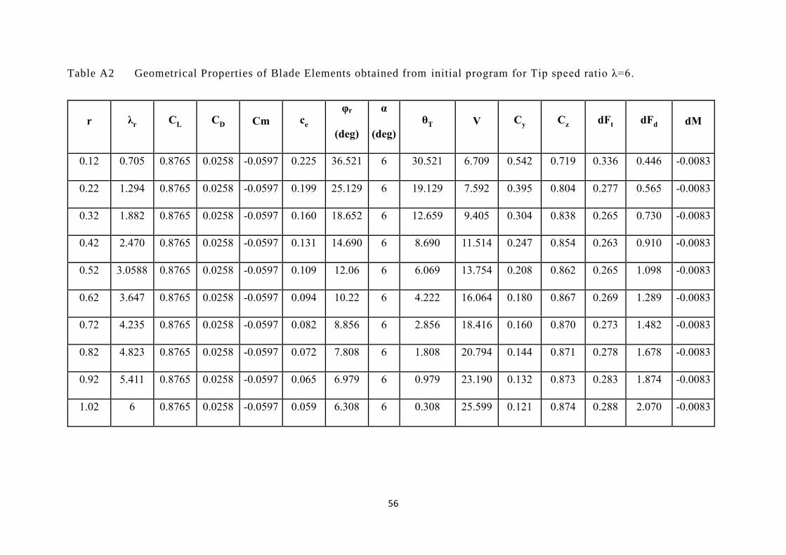
56
Table A2 Geometrical Properties of Blade Elements obtained from initial program for Tip speed ratio λ=6.
r λr C
L C
D Cm c
e
φr
(deg)
α
(deg)
θT V C
y C
z dF
t dF
d dM
0.12 0.705 0.8765 0.0258 -0.0597 0.225 36.521 6 30.521 6.709 0.542 0.719 0.336 0.446 -0.0083
0.22 1.294 0.8765 0.0258 -0.0597 0.199 25.129 6 19.129 7.592 0.395 0.804 0.277 0.565 -0.0083
0.32 1.882 0.8765 0.0258 -0.0597 0.160 18.652 6 12.659 9.405 0.304 0.838 0.265 0.730 -0.0083
0.42 2.470 0.8765 0.0258 -0.0597 0.131 14.690 6 8.690 11.514 0.247 0.854 0.263 0.910 -0.0083
0.52 3.0588 0.8765 0.0258 -0.0597 0.109 12.06 6 6.069 13.754 0.208 0.862 0.265 1.098 -0.0083
0.62 3.647 0.8765 0.0258 -0.0597 0.094 10.22 6 4.222 16.064 0.180 0.867 0.269 1.289 -0.0083
0.72 4.235 0.8765 0.0258 -0.0597 0.082 8.856 6 2.856 18.416 0.160 0.870 0.273 1.482 -0.0083
0.82 4.823 0.8765 0.0258 -0.0597 0.072 7.808 6 1.808 20.794 0.144 0.871 0.278 1.678 -0.0083
0.92 5.411 0.8765 0.0258 -0.0597 0.065 6.979 6 0.979 23.190 0.132 0.873 0.283 1.874 -0.0083
1.02 6 0.8765 0.0258 -0.0597 0.059 6.308 6 0.308 25.599 0.121 0.874 0.288 2.070 -0.0083

57
Table A3 Geometrical Properties of Blade Elements obtained from initial program for Tip speed ratio λ=7.
r λr C
L C
D Cm c
e
φr
(deg)
α
(deg)
θT V C
y C
z dF
t dF
d dM
0.12 0.8235 0.8765 0.0258 -0.0597 0.1925 33.685 6 27.685 7.8467 0.5075 0.7436 0.3686 0.5400 -0.0083
0.22 1.5098 0.8765 0.0258 -0.0597 0.1578 22.345 6 16.345 9.5701 0.3570 0.8204 0.3163 0.7267 -0.0083
0.32 2.1960 0.8765 0.0258 -0.0597 0.1232 16.321 6 10.321 12.259 0.2710 0.8484 0.3075 0.9626 -0.0083
0.42 2.8823 0.8765 0.0258 -0.0597 0.0990 12.755 6 6.7557 15.252 0.2186 0.8605 0.3087 1.2148 -0.0083
0.52 3.5686 0.8765 0.0258 -0.0597 0.0822 10.435 6 4.4359 18.379 0.1841 0.8666 0.3132 1.4743 -0.0083
0.62 4.2549 0.8765 0.0258 -0.0597 0.0700 8.8172 6 2.8172 21.577 0.1598 0.8700 0.3192 1.7376 -0.0083
0.72 4.9411 0.8765 0.0258 -0.0597 0.0608 7.6273 6 1.6273 24.817 0.1419 0.8721 0.3259 2.0033 -0.0083
0.82 5.6274 0.8765 0.0258 -0.0597 0.0538 6.7175 6 0.7175 28.084 0.1281 0.8735 0.3331 2.2705 -0.0083
0.92 6.3137 0.8765 0.0258 -0.0597 0.0481 6.0000 6 0.3512 31.36 0.1172 0.8743 0.3405 2.5387 -0.0083
1.02 7 0.8765 0.0258 -0.0597 0.0435 5.4200 6 0 34.666 0.1084 0.8750 0.3480 2.8075 -0.0083

58
Appendix III
Newmark Time Integration scheme
Time Integration schemes are methods to find the discrete time responses.
Newmark method of time integration belongs to discrete time interval type where
the discrete time responses are obtained by giving input of the Global Mass,
Stiffness, Damping Matrices and Force vectors as inputs for solving the time
domain response.
The Velocity is expressed as:
tXXXX dttntntdtt )1( (A.8)
The Displacement is expressed as:
dtttttdtt XXtXXX
2
1 (A.9)
The governing differential equations will be:
dttdttedttedtte FXKXCXM (A.10)
The procedure to develop the Velocity and Acceleration responses is as shown
below:
Step 1:
The Mass[M]e, Stiffness[K]e and Coupling matrices[C]e are taken.
Step 2:

59
The values of initial displacement X0 and velocity 0X are given.
Step 3:
By choosing the values of dt, α and δn, the values of constants a0 to a7 are
calculated as:
21
dtao
,
dta n
1
, dt
a
12 , 1
2
13
a ,
14
na ,
2
25
ndta and )1(6 ndta
Step 4:
Form the effective stiffness matrix and effective load matrix as:
][][][][ 10 CaMaKKeff (A.11)
)]([]([ 541320 tttttttdtt XaXaXaCXaXaXaMff
Step 5:
Solve [ 1
dtteffdtt fKX
Step 6:
The acceleration and velocities at time t+dt can be written as:
tttdttdtt XaXaXXaX 320
(A.12)
dttttdtt XaXaXX 76 (A.13)

60
Appendix IV
MATLAB codes of the computations done to find out the Geometric Mass,
Stiffness matrices and Global Force vector, are presented below. Then code for
conducting Newmark Integration to get dynamic response spectrum is also
explained below.
III.1 MATLAB Code to Compute Global Mass and Stiffness Matrices
%Function to compute global Mass and Stiffness Matrices function[GMr,GKr]=Global_Mass_Stiffness215() clc clear all
%Initialize the parameters such as Length, Area, Young’s Modulus, density
of each blade element, A=[8.36529 42.39464 30.70165 20.19344 13.74556 9.815455 7.311195 5.63727
4.47042 3.627475]*1e-4; E=6*1e9;den=1400; L=[12 10 10 10 10 10 10 10 10 10]*1e-2; Iz=[5.56868 738.1311 450.626805 203.71994 95.493375 48.53348 26.79224
16.04464 10.07106 6.61904]*1e-8; Iy=[5.56868 196.0412 53.74758 13.28684 4.2068 1.94449 1.071425 0.45722
0.278195 0.18105]*1e-8; Iyz=[0 339.0584 130.5248 38.01509 11.8492 5.248325 2.661715 0.519385
0.15931 0.017845]*1e-8; G=2.5424*1e9; J=[11.13736 66.25 53.38538 94.18572 72.81243 55.32523 41.51267 30.71831
22.44229 16.11037 11.59907 8.17581]*1e-8; GK=zeros(66,66);Gks=zeros(66,66);GM=zeros(66,66);GMs=zeros(66,66);
a=zeros(length(A));b=zeros(12);c=zeros(12);d=zeros(12);e=zeros(12);f=zeros(
12);g=zeros(12);h=zeros(12);i1=zeros(12);j=zeros(12);
for i=1:length(A)
a=(A(i)*E)/L(i); b=(12*E*Iz(i))/(L(i)^3); c=(6*E*Iz(i))/(L(i)^2); d=(12*E*Iy(i))/(L(i)^3); e=(6*E*Iy(i))/(L(i)^2); f=G*J(i)/L(i); g=4*E*Iy(i)/L(i); h=2*E*Iy(i)/L(i); i1=4*E*Iz(i)/L(i); j=2*E*Iz(i)/L(i); l=(12*E*Iyz(i))/(L(i)^3); m=(6*E*Iyz(i))/(L(i)^2); n=(4*E*Iyz(i))/L(i); o=(2*E*Iyz(i))/L(i);

61
K=[a 0 0 0 0 0 -a 0 0 0 0 0; 0 b l 0 -m c 0 -b -l 0 -m c;0 l d 0 -e m 0
-l -d 0 -e m;0 0 0 f 0 0 0 0 0 -f 0 0;0 -m -e 0 g -n 0 m e 0 h -o;0 c m 0 -
n i1 0 -c -m 0 -o j;-a 0 0 0 0 0 a 0 0 0 0 0;0 -b -l 0 m -c 0 b l 0 m -c;0
-l -d 0 e -m 0 l d 0 e -m;0 0 0 -f 0 0 0 0 0 f 0 0;0 -m -e 0 h -o 0 m e 0 g
-n;0 c m 0 -o j 0 -c -m 0 -n i1];
r=(i-1)*6+1; Gks(r:r+11,r:r+11)=K; GK=GK+Gks; Gks=zeros(66,66); end
for i=1:length(A)
a=1/3; b=13/35; c=(Iy(i)+Iz(i))/(3*A(i)); d=L(i)^2/105; e=(11*L(i))/210; f=1/6; g=9/70; h=(13*L(i))/420; j=(Iy(i)+Iz(i))/(6*A(i)); l=L(i)^2/140; area=A(i);leng=L(i); M=[a 0 0 0 0 0 f 0 0 0 0 0;0 b 0 0 0 e 0 g 0 0 0 -h;0 0 b 0 -e 0 0 0 g
0 h 0;0 0 0 c 0 0 0 0 0 j 0 0;0 0 -e 0 d 0 0 0 -h 0 -l 0;0 e 0 0 0 d 0 h 0
0 0 -l;f 0 0 0 0 0 a 0 0 0 0 0;0 g 0 0 0 h 0 b 0 0 0 -e;0 0 g 0 -h 0 0 0 b
0 e 0;0 0 0 j 0 0 0 0 0 c 0 0;0 0 h 0 -l 0 0 0 e 0 d 0;0 h 0 0 0 -l 0 -e 0
0 0 d]*(den*area*leng); r=(i-1)*6+1; GMs(r:r+11,r:r+11)=M; GM=GM+GMs; GMs=zeros(66,66);
end
GKr=zeros(61,61);GMr=zeros(61,61);
%Gkr and Gmr are the reduced matrices after giving initial boundary %conditions
for i=6:66 for j=6:66 GKr(i-5,j-5)=GK(i,j); GMr(i-5,j-5)=GM(i,j); end end
III.2 Function to Compute Globalized Force Vector
%Function to compute the global force vector function[GFv]=global_force215() clear all clc dt=0.001;T=1; F=zeros(12,1);GFv=zeros(61,length(dt:dt:T));

62
count=1; for t=dt:dt:T
GFv(:,count)=force_gen215(t); count=count+1; end %function to generate generalized force vector for a particular time period function[GFr]=force_gen215(t) A=[8.36529 42.39464 30.70165 20.19344 13.74556 9.815455 7.311195 5.63727
4.47042 3.627475]*1e-4; L=[12 10 10 10 10 10 10 10 10 10]*1e-2; den_a=1.225;den=1400; ome=50; x=[0 0.12 0.22 0.32 0.42 0.52 0.62 0.72 0.82 0.92 1.02]; g=9.81; Fks=zeros(66,1);GFv=zeros(66,1); Cy=[0 0.468969449 0.350179036 0.276010116 0.227869405 0.194719307
0.170689529 0.152540617 0.138378381 0.127033037]; Cz=[0 0.762117034 0.821603907 0.846550333 0.858454545 0.864843104
0.868593723 0.870949967 0.872509192 0.873583902]; c=[1.631795 21.21254432 17.98410485 14.59462041 12.05483529 10.19619802
8.805764814 7.736053205 6.891462789 6.209478139]*1e-2; Vr=[0 6.709276501 7.592497881 9.405770927 11.51439555 13.75465549
16.06476931 18.41629808 20.79435991 23.1904253 25.59925995]; Cm=[0 -0.0597 -0.0597 -0.0597 -0.0597 -0.0597 -0.0597 -0.0597 -0.0597 -
0.0597]; Iyz=[0 339.058415 130.524795 38.01509 11.8492 5.248325 2.661715 0.519385
0.15931 0.017845]*1e-8;
for i=1:length(A)
if i==1 F=zeros(12,1); else ti=ome*t*pi/180; a=(1/6)*den*L(i)*ome*ome*A(i)*(2*x(i)+x(i+1))-
0.5*den*g*L(i)*A(i)*sin(ti); b=(1/4)*den_a*L(i)*Cy(i)*c(i)*Vr(i)*Vr(i)-
0.5*den*g*L(i)*A(i)*cos(ti); d=(1/4)*den_a*L(i)*Cz(i)*c(i)*Vr(i)*Vr(i); e=(1/4)*den_a*L(i)*Cm(i)*c(i)*c(i)*Vr(i)*Vr(i)-
0.5*den*L(i)*ome*ome*Iyz(i); f=0; h=0; j=(1/6)*den*L(i)*ome*ome*A(i)*(x(i)+2*x(i+1))-
0.5*den*g*L(i)*A(i)*sin(ti); k=(1/4)*den_a*L(i)*Cy(i)*c(i)*Vr(i)*Vr(i)-
0.5*den*g*L(i)*A(i)*cos(ti); l=(1/4)*den_a*L(i)*Cz(i)*c(i)*Vr(i)*Vr(i); m=(1/4)*den_a*L(i)*Cm(i)*c(i)*c(i)*Vr(i)*Vr(i)-
0.5*den*L(i)*ome*ome*Iyz(i); n=0; o=0;
F= [a;b;d;e;f;h;j;k;l;m;n;o]; end
rec=(i-1)*6+1; Fks(rec:rec+11,1)=F; GFv=GFv+Fks;

63
Fks=zeros(66,1); end
GFr=zeros(61,1);
for i=6:66 GFr(i-5,1)=GFv(i,1); end
III.3 Program of Implementing Newmark Method to conduct Dynamic Response
Analysis
%Program to conduct Newmark Double Integration Analysis to find out %Frequency Reponse of the Blade acted upon by various loads. clc clear all dt=0.001; T=1; GF=zeros(61,length(dt:dt:T)); GM=zeros(61,61); GK=zeros(61,61);F0=zeros(61,1);
[GM,GK]=Global_Mass_Stiffness215(); GF=global_force215(); F0=force_gen215(0); X0=zeros(61,1); X0d=zeros(61,1); X0dd=inv(GM)*(F0-GK*X0);
delta=0.5; alpha=0.25*(0.5+delta)^2; c0=1/(alpha*dt*dt); c1=delta/(alpha*dt); c2=1/(alpha*dt); c3=1/(2*alpha)-1; c4=delta/alpha-1; c5=(dt*(delta/alpha-2))/2; c6=dt*(1-delta); c7=delta*dt;
Keff=zeros(60,60); Keff=GK+c0*GM; Kinv=inv(Keff);
i=1; X(:,1)=X0; Xd(:,1)=X0d; Xdd(:,1)=X0dd; t=0;
for t=dt:dt:T
i=i+1; F=GF(:,i-1); Feff=F+GM*(c0*X(:,i-1)+c2*Xd(:,i-1)+c3*Xdd(:,i-1));
X(:,i)=Kinv*Feff; Xdd(:,i)=c0*(X(:,i)-X(:,i-1))-c2*Xd(:,i-1)-c3*Xdd(:,i-1);

64
Xd(:,i)=Xd(:,i-1)+c6*(Xdd(:,i-1))+c7*Xdd(:,i);
F=zeros(61,1);Feff=zeros(61,1); end
N=length(0:0.001:1); fs=30;%62.5 samples per second fnyquist=fs/2; %Nyquist frequency X_mags=abs(fft(X(56,:))); bin_vals=[0:N-1]; fax_Hz=bin_vals*fs/N; N_2=ceil(N/2);
subplot(2,1,1)
plot(fax_Hz(1:N_2),X_mags(1:N_2)) xlabel('Frequency HZ') ylabel('Magnitude') title('Single sided maginitude spectrum'); axis tight
subplot(2,1,2) plot(0:dt:T,X(58,:)); xlabel('time (in sec)') ylabel('flexure angle response gamma') title('Flapwise beating at the blade end') axis tight