modelling mimo systems in body area networks in...
TRANSCRIPT

UNIVERSIDADE TÉCNICA DE LISBOAINSTITUTO SUPERIOR TÉCNICO
Modelling MIMO Systems inBody Area Networks in Outdoors
Michał Łukasz Maćkowiak
X Supervisor: Doctor Luís Manuel de Jesus Sousa Correia
Thesis approved in public session to obtain thePh.D. Degree in Electrical and Computer Engineering
Jury final classification: Pass with Merit
Jury
X Chairperson: Chairman of the IST Scientific BoardX Members of the Committee:
X Doctor Alain SibilleX Doctor Jorge Manuel Lopes Leal Rodrigues da CostaX Doctor Luís Manuel de Jesus Sousa CorreiaX Doctor Custódio José de Oliveira PeixeiroX Doctor António José Castelo Branco Rodrigues
2013

x

UNIVERSIDADE TÉCNICA DE LISBOAINSTITUTO SUPERIOR TÉCNICO
Modelling MIMO Systems inBody Area Networks in Outdoors
Michał Łukasz Maćkowiak
X Supervisor: Doctor Luís Manuel de Jesus Sousa Correia
Thesis approved in public session to obtain thePh.D. Degree in Electrical and Computer Engineering
Jury final classification: Pass with Merit
Jury
Chairperson: Chairman of the IST Scientific BoardMembers of the Committee:Doctor Alain Sibille, Full Professor, Télécom Paris Tech, FrançaDoctor Jorge Manuel Lopes Leal Rodrigues da Costa, Professor Associado
(com Agregação), do Instituto Superior de Ciências do Trabalho e daEmpresa do Instituto Universitário de Lisboa
Doctor Luís Manuel de Jesus Sousa Correia, Professor Associado (com Agregação)do Instituto Superior Técnico, da Universidade Técnica de Lisboa
Doctor Custódio José de Oliveira Peixeiro, Professor Auxiliar do Instituto SuperiorTécnico, da Universidade Técnica de Lisboa
Doctor António José Castelo Branco Rodrigues, Professor Auxiliar do InstitutoSuperior Técnico, da Universidade Técnica de Lisboa
Funding Institution:Fundação para a Ciência e a Tecnologia
2013

x

x
to my beloved
Hania, Zosia and Leon

x

Modelling MIMO Systems in Body Area Networks in Outdoors
Acknowledgements
In the first place, I would like to express my deep gratitude to Professor Luis M. Correia,for patient guidance, enthusiastic encouragement, corrections and great help during mywork and stay in Portugal. His broad experience, unconditional support and many usefulcritiques of this research work allowed to keep my progress on schedule.
My grateful thanks are also extended to Carla Oliveira for her friendship, productiveideas, a very effective cooperation and fruitful discussions throughout this work.
I would like to express my gratitude to all members of GROW and my colleagues fromIST-TUL, for their support and sharing of ideas.
My gratitude to IST, for the logistics provided that made this thesis possible.
I also thank FCT for the scholarship and for all the financial support.
I would like to thank the European Commission for financing the projects in which Iwas involved during the period of this thesis, which are: COST 2100, COST IC1004,NEWCOM++, NEWCOM, LEXNET.
I am also grateful to all my friends, for their kind support.
I send my special acknowledgements to my parents, for their lifetime support and enco-uragement in what I did.
My grateful thanks are also extended to my brother, and rest of my family in Poland,because I can always count on them.
Above all, I wish to express my deep gratitude to my beloved wife Hania and my wonderfulchildren Zosia and Leon.
v

x

Modelling MIMO Systems in Body Area Networks in Outdoors
Abstract
The aim of this work is to develop a radio channel model for MIMO systems appliedto Body Area Networks for off-body radio links in a multipath environment. Firstly,the influence of the body on antenna performance has been evaluated. Then, the bodydynamics were taken into account and model based on Motion Capture data has beendeveloped. Finally, the propagation environment has been modelled using GeometricallyBased Statistic Channel model. A patch antenna operating at 2.45 GHz is simulated inComputer Simulation Technology, near to a voxel model. Multi-Path Components areobtained for a street scenario, for a running or walking body, and for various on-bodyantenna placements. The propagation conditions are determined and statistics of basicchannel parameters are calculated. Moreover, the analysis of MIMO capacity are per-formed and the optimum location of antennas are selected. The influence of the body isthe highest when the antenna is attached to the body. Gain patterns are significantlymodified by the body movement, as well as channel parameters. For the running body,when the antenna is located on the arm, 9 dB deep fades in the average received powerare captured. The MIMO capacity strongly depends on the power imbalance betweenantennas.
KeywordsChannel Models. MIMO. Body Area Networks. Body Dynamics. Wearable Antennas.Statistical Modelling. Delay Spread. Angular Spread. Capacity. Performance.
vii

Streszczenie
Streszczenie
Celem rozprawy doktorskiej jest opracowanie modelu kanału radiowego, dla systemuMIMO zastosowanego w sieciach nasobnych (Body Area Networks) pracujących w wie-lodrogowym środowisku propagacyjnym. W pierwszej kolejności został uwzględnionywpływ tkanek człowieka na parametry anteny umieszczonej na ciele. Następnie, bazującna opisie ruchu (Motion Capture) została uwzględniona dynamika ciała. Środowiskopropagacyjne zostało zamodelowane za pomocą geometrycznego modelu stochastycznego(Geometrically Based Statistic Channel). Antena nasobna, pracująca w paśmie 2.45 GHzzostała zasymulowana w programie CST (Computer Simulation Technology) przy użyciuwokselowego modelu człowieka. W pracy przedstawiono statystyczną analizę parametrówkanału radiowego (scenariusz ulicy), dla wielu anten umieszczonych na poruszającym sięczłowieku (chód i bieg). Ponadto, obliczona została pojemność systemu MIMO orazwybrano optymalne położenie anten nasobnych w analizowanym scenariuszu. Wpływtkanek człowieka jest najbardziej widoczny gdy antena jest umieszczona bezpośredniona ciele. Dominujący wpływ na zmianę charakterystyki promieniowania anteny orazparametry kanału radiowego ma ruch człowieka. W przypadku biegu oraz gdy antenaumieszczona jest na nadgarstku, zarejestrowano wahania w poziomie odbieranego sygnałuo 9 dB. Pojemność systemu MIMO zależy w głównej mierze od balansu poziomu mocyodbieranego sygnału przez anteny.
Słowa KluczoweModelowanie Kanalow Radiowych. MIMO. Sieci Nasobne. Dynamika Ciała Człowieka.Modelowanie Statystyczne. Rozproszenie Opóźnienia. Rozproszenie Kątowe. Zysk Po-jemność. Analiza Wydajności.
viii

Modelling MIMO Systems in Body Area Networks in Outdoors
Resumo
O objectivo deste trabalho é o desenvolvimento de um modelo de canal aplicado àsredes de sensores corporais, usando MIMO, para ligações com o exterior em ambientemulti-percurso. Começou por se estudar a influência do utilizador no desempenho daantena corporal. Considerou-se a mobilidade deste, criando-se um modelo baseado nacaptura do movimento. O ambiente de propagação foi incluído através de um modelogeométrico e estatístico do canal. Usou-se o simulador CST para estudar o desempenhode um patch a 2.45 GHz, junto a um modelo voxel. Obtiveram-se as componentesmulti-percurso para o cenário de um utilizador com várias antenas, a caminhar ou acorrer numa estrada. Analisaram-se as condições de propagação e as estatísticas dos pa-râmetros básicos do canal rádio. Com base nos valores obtidos para a capacidade MIMO,identificaram-se as melhores localizações para as antenas. Verificou-se que a influênciado utilizador é maior quando a antena está em contacto com este. A mobilidade alterasignificativamente os diagramas de radiação e os parâmetros do canal rádio. Por exem-plo, podem ocorrer desvanecimentos de 9 dB, durante uma corrida em que o utilizadorusa uma antena no pulso. Verificou-se que a capacidade MIMO depende fortemente dobalanço de potência entre as antenas.
Palavras-chaveModelos de Canal. MIMO. Redes de Sensores Corporais. Mobilidade. Antenas Cor-porais. Modelação Estatística. Variação do Atraso. Variação Angular. Capacidade.Desempenho.
ix

x

Conteúdo
Table of Contents
Acknowledgements . . . . . . . . . . . . . . . . . . . . . . . . . . . . . . . . . . . . . v
Abstract . . . . . . . . . . . . . . . . . . . . . . . . . . . . . . . . . . . . . . . . . . . . vii
Streszczenie . . . . . . . . . . . . . . . . . . . . . . . . . . . . . . . . . . . . . . . . . viii
Resumo . . . . . . . . . . . . . . . . . . . . . . . . . . . . . . . . . . . . . . . . . . . . ix
Table of Contents . . . . . . . . . . . . . . . . . . . . . . . . . . . . . . . . . . . . . xi
List of Figures . . . . . . . . . . . . . . . . . . . . . . . . . . . . . . . . . . . . . . . . xiii
List of Tables . . . . . . . . . . . . . . . . . . . . . . . . . . . . . . . . . . . . . . . . xviii
List of Acronyms . . . . . . . . . . . . . . . . . . . . . . . . . . . . . . . . . . . . . . xx
List of Symbols . . . . . . . . . . . . . . . . . . . . . . . . . . . . . . . . . . . . . . . xxiii
List of Software . . . . . . . . . . . . . . . . . . . . . . . . . . . . . . . . . . . . . . . xxxi
Chapter 1. Introduction . . . . . . . . . . . . . . . . . . . . . . . . . . . . . . . . . . 1
1.1. Motivations . . . . . . . . . . . . . . . . . . . . . . . . . . . . . . . . . . . . . . . . 2
1.2. Novelty . . . . . . . . . . . . . . . . . . . . . . . . . . . . . . . . . . . . . . . . . . 4
1.3. Research Strategy and Impact . . . . . . . . . . . . . . . . . . . . . . . . . . . . . 5
1.4. Structure of the Dissertation . . . . . . . . . . . . . . . . . . . . . . . . . . . . . . 8
Chapter 2. MIMO Channel Models . . . . . . . . . . . . . . . . . . . . . . . . . . 11
2.1. Channel Description . . . . . . . . . . . . . . . . . . . . . . . . . . . . . . . . . . . 12
2.2. Wideband Channel Models . . . . . . . . . . . . . . . . . . . . . . . . . . . . . . . 14
2.3. Channel Parameters . . . . . . . . . . . . . . . . . . . . . . . . . . . . . . . . . . . 17
2.4. MIMO Channel . . . . . . . . . . . . . . . . . . . . . . . . . . . . . . . . . . . . . . 19
2.5. Boundary Conditions . . . . . . . . . . . . . . . . . . . . . . . . . . . . . . . . . . 21
Chapter 3. Body Area Networks . . . . . . . . . . . . . . . . . . . . . . . . . . . . 23
3.1. Body Area Network Channel . . . . . . . . . . . . . . . . . . . . . . . . . . . . . . 24
3.2. Body Modelling . . . . . . . . . . . . . . . . . . . . . . . . . . . . . . . . . . . . . 28
3.3. Wearable Antennas . . . . . . . . . . . . . . . . . . . . . . . . . . . . . . . . . . . . 30
3.4. Numerical Modelling Techniques . . . . . . . . . . . . . . . . . . . . . . . . . . . . 32
Chapter 4. Statistical Modelling of Antennas on a Body . . . . . . . . . . . 39
4.1. Concept and Scenarios . . . . . . . . . . . . . . . . . . . . . . . . . . . . . . . . . . 40
4.2. Theoretical Model . . . . . . . . . . . . . . . . . . . . . . . . . . . . . . . . . . . . 43
4.3. Numerical Model . . . . . . . . . . . . . . . . . . . . . . . . . . . . . . . . . . . . . 45
4.4. Modelling of Signal Correlation . . . . . . . . . . . . . . . . . . . . . . . . . . . . . 50
4.5. Modelling of Body Dynamics . . . . . . . . . . . . . . . . . . . . . . . . . . . . . . 52
xi

Table of Contents
Chapter 5. Results of Statistical Behaviour of Antennas on a Body . . . . 57
5.1. Body Coupling . . . . . . . . . . . . . . . . . . . . . . . . . . . . . . . . . . . . . . 58
5.1.1. Theoretical Approach . . . . . . . . . . . . . . . . . . . . . . . . . . . . . . . . 58
5.1.2. Numerical Approach . . . . . . . . . . . . . . . . . . . . . . . . . . . . . . . . . 62
5.1.3. Experiment . . . . . . . . . . . . . . . . . . . . . . . . . . . . . . . . . . . . . . 66
5.2. Signal Correlation . . . . . . . . . . . . . . . . . . . . . . . . . . . . . . . . . . . . 69
5.3. Body Dynamics . . . . . . . . . . . . . . . . . . . . . . . . . . . . . . . . . . . . . . 73
Chapter 6. Channel Model . . . . . . . . . . . . . . . . . . . . . . . . . . . . . . . . 81
6.1. Concept and Parameters . . . . . . . . . . . . . . . . . . . . . . . . . . . . . . . . . 82
6.2. Model Implementation . . . . . . . . . . . . . . . . . . . . . . . . . . . . . . . . . . 85
6.3. Model Assessment . . . . . . . . . . . . . . . . . . . . . . . . . . . . . . . . . . . . 87
6.4. Scenarios . . . . . . . . . . . . . . . . . . . . . . . . . . . . . . . . . . . . . . . . . 89
Chapter 7. MIMO Capacity in BANs . . . . . . . . . . . . . . . . . . . . . . . . 91
7.1. Radio Channel Parameters . . . . . . . . . . . . . . . . . . . . . . . . . . . . . . . 92
7.1.1. Propagation Conditions . . . . . . . . . . . . . . . . . . . . . . . . . . . . . . . 92
7.1.2. Received Power . . . . . . . . . . . . . . . . . . . . . . . . . . . . . . . . . . . 93
7.1.3. Delay Spread . . . . . . . . . . . . . . . . . . . . . . . . . . . . . . . . . . . . . 94
7.1.4. Spread of the Direction of Arrival . . . . . . . . . . . . . . . . . . . . . . . . . 95
7.1.5. Correlation between Received Signal Envelopes . . . . . . . . . . . . . . . . . . 96
7.1.6. Correlation between Channel Impulse Responses . . . . . . . . . . . . . . . . . 97
7.2. MIMO Capacity . . . . . . . . . . . . . . . . . . . . . . . . . . . . . . . . . . . . . 99
7.3. Optimum Antenna Placement . . . . . . . . . . . . . . . . . . . . . . . . . . . . . . 103
Chapter 8. Conclusions . . . . . . . . . . . . . . . . . . . . . . . . . . . . . . . . . . 107
8.1. Summary . . . . . . . . . . . . . . . . . . . . . . . . . . . . . . . . . . . . . . . . . 108
8.2. Main Results . . . . . . . . . . . . . . . . . . . . . . . . . . . . . . . . . . . . . . . 109
8.3. Future Work . . . . . . . . . . . . . . . . . . . . . . . . . . . . . . . . . . . . . . . 113
Annex A. User’s Manual . . . . . . . . . . . . . . . . . . . . . . . . . . . . . . . . . 115
Annex B. Tissues Properties . . . . . . . . . . . . . . . . . . . . . . . . . . . . . . . 119
Annex C. CST Simulations . . . . . . . . . . . . . . . . . . . . . . . . . . . . . . . . 120
Annex D. Body Dynamics . . . . . . . . . . . . . . . . . . . . . . . . . . . . . . . . 124
Annex E. Radio Channel Parameters . . . . . . . . . . . . . . . . . . . . . . . . . 132
Annex F. MIMO Capacity . . . . . . . . . . . . . . . . . . . . . . . . . . . . . . . . 139
Annex G. MIMO Performance . . . . . . . . . . . . . . . . . . . . . . . . . . . . . 161
References . . . . . . . . . . . . . . . . . . . . . . . . . . . . . . . . . . . . . . . . . . . 165

Modelling MIMO Systems in Body Area Networks in Outdoors
List of Figures
1.1. Body Centric Wireless Communications. . . . . . . . . . . . . . . . . . . . . . . . . . 3
1.2. Thesis framework. . . . . . . . . . . . . . . . . . . . . . . . . . . . . . . . . . . . . . 5
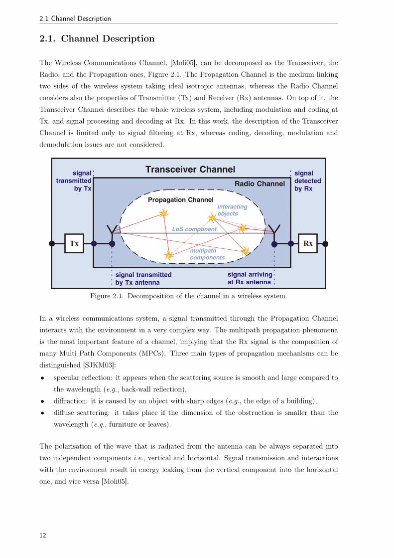
2.1. Decomposition of the channel in a wireless system. . . . . . . . . . . . . . . . . . . . 12
2.2. Signal path loss and fading. . . . . . . . . . . . . . . . . . . . . . . . . . . . . . . . . 14
2.3. Multibounce signal processed by Rx. . . . . . . . . . . . . . . . . . . . . . . . . . . . 14
2.4. MIMO system. . . . . . . . . . . . . . . . . . . . . . . . . . . . . . . . . . . . . . . . 19
2.5. Dielectric boundary conditions. . . . . . . . . . . . . . . . . . . . . . . . . . . . . . . 21
3.1. Parts of transmission channel of SISO off-body system. . . . . . . . . . . . . . . . . 25
3.2. Virtual MIMO for off-body communications. . . . . . . . . . . . . . . . . . . . . . . 27
3.3. Body tissues permittivity and conductivity for 915 MHz, 2.45 GHz and 5.8 GHz. . . 29
3.4. Virtual Family models (based on data taken from [Chri10]). . . . . . . . . . . . . . . 30
3.5. Wearable antennas integrated into a firefighter jacket (extracted from [VTHR10]). . 30
3.6. Division of calculation domain into grids in FIT (extracted from [CST12]). . . . . . 33
3.7. Automatic mesh generation procedure in one direction. . . . . . . . . . . . . . . . . 36
4.1. Statistical modelling of antennas on a body. . . . . . . . . . . . . . . . . . . . . . . . 40
4.2. Body segmentation and orientation. . . . . . . . . . . . . . . . . . . . . . . . . . . . 41
4.3. Motion Capture snap-shot frames of the body movement (extracted from [POSE12]). 42
4.4. Patch antenna with switchable slots in a closed configuration [MCCF07]. . . . . . . 42
4.5. Model for the estimation of the radiation pattern of the electric field of an antenna
located over infinite lossy dielectric half space. . . . . . . . . . . . . . . . . . . . . . 44
4.6. Simple model for the estimation of the radiation pattern of the electric field of an
antenna located in the vicinity of a body. . . . . . . . . . . . . . . . . . . . . . . . . 44
4.7. Numerical model for an antenna placed near the head (voxel head extracted from
[Chri10]). . . . . . . . . . . . . . . . . . . . . . . . . . . . . . . . . . . . . . . . . . . 45
4.8. Comparison of S11 curves for patch antenna calculated for various meshing
parameters. . . . . . . . . . . . . . . . . . . . . . . . . . . . . . . . . . . . . . . . . . 50
4.9. Relative error of patch antenna parameters for various meshing scenarios. . . . . . . 50
4.10. Correlation Model. . . . . . . . . . . . . . . . . . . . . . . . . . . . . . . . . . . . . . 51
4.11. Body directions, in the usual spherical coordinates system. . . . . . . . . . . . . . . 53
5.1. The radiation pattern of the normalized electric field of an antenna located over an
infinite half space, for electric properties set to the values of the 2/3 Muscle Model,
2.45 GHz, and parallel polarisation. . . . . . . . . . . . . . . . . . . . . . . . . . . . 58
5.2. The average radiation pattern of electric field of antenna located over infinite
half space, for electric properties set to the values of the 2/3 Muscle Model, for
915 MHz, for parallel polarisation. . . . . . . . . . . . . . . . . . . . . . . . . . . . . 59
xiii

List of Figures
5.3. Comparison of standard deviations for parallel polarisation, 915 MHz and 5.8 GHz,
2/3 Muscle tissue, and Torso position. . . . . . . . . . . . . . . . . . . . . . . . . . . 60
5.4. Comparison of standard deviation for parallel polarisation, Fat and Muscle tissues,
2.45 GHz, and Torso position. . . . . . . . . . . . . . . . . . . . . . . . . . . . . . . 61
5.5. Comparison of average radiation pattern for the Rayleigh Distribution, for various
positions on the body. . . . . . . . . . . . . . . . . . . . . . . . . . . . . . . . . . . . 61
5.6. Gain patterns of a patch antenna for various distances to the Head. . . . . . . . . . 63
5.7. PWD for all analysed body regions for a distance range of [0, 2λ] at 2.45 GHz. . . . 63
5.8. Statistics of the gain pattern of the antenna located near the Head for Uniform and
Rayleigh Distributions relative to the gain pattern of the isolated antenna. . . . . . 64
5.9. Comparison of the average gain patterns, for the Rayleigh Distribution, and various
body regions. . . . . . . . . . . . . . . . . . . . . . . . . . . . . . . . . . . . . . . . . 65
5.10. Measurement setup. . . . . . . . . . . . . . . . . . . . . . . . . . . . . . . . . . . . . 66
5.11. Measurement environment. . . . . . . . . . . . . . . . . . . . . . . . . . . . . . . . . 67
5.12. Average radiation patterns for various distances. . . . . . . . . . . . . . . . . . . . . 67
5.13. Statistics of the measured gain pattern of the antenna located near the Chest,
relative to the isolated one. . . . . . . . . . . . . . . . . . . . . . . . . . . . . . . . . 68
5.14. Comparison between CST and measurements. . . . . . . . . . . . . . . . . . . . . . . 69
5.15. Average and standard deviation of cross-correlation for the various classes. . . . . . . 71
5.16. Average and standard deviation of cross-correlation for selected pairs of antennas. . 71
5.17. Standard deviation of correlation for the several classes, for various directions of
the incoming wave. . . . . . . . . . . . . . . . . . . . . . . . . . . . . . . . . . . . . . 72
5.18. The average and standard deviation of cross-correlation for the various classes, for
several distances from the body. . . . . . . . . . . . . . . . . . . . . . . . . . . . . . 73
5.19. The normal to the body surface of a wearable antenna placed on the Arm, for the
walking or running bodies. . . . . . . . . . . . . . . . . . . . . . . . . . . . . . . . . 74
5.20. Average and range of change in the normal to the body surface of a wearable
antenna for the walking or running bodies. . . . . . . . . . . . . . . . . . . . . . . . 74
5.21. Standard deviation of change in normal to the body surface for walking and running
bodies. . . . . . . . . . . . . . . . . . . . . . . . . . . . . . . . . . . . . . . . . . . . 75
5.22. Histograms and distribution fitting of the normal direction to the body surface for
the running body in the azimuth plane. . . . . . . . . . . . . . . . . . . . . . . . . . 75
5.23. Placements and gains of the antenna on the static body. . . . . . . . . . . . . . . . . 77
5.24. Statistics of the gain pattern of the patch antenna placed on the Arm for the
running body. . . . . . . . . . . . . . . . . . . . . . . . . . . . . . . . . . . . . . . . 77
5.25. Comparison of average gain patterns for the running body. . . . . . . . . . . . . . . 79
5.26. Antenna located on the Arm. . . . . . . . . . . . . . . . . . . . . . . . . . . . . . . . 79
5.27. Average radiation pattern for the Arm placement and the walking body. . . . . . . . 80
6.1. Modelling concept of off-body Radio Channel. . . . . . . . . . . . . . . . . . . . . . 82
6.2. Structure of the simulator. . . . . . . . . . . . . . . . . . . . . . . . . . . . . . . . . 85
xiv

Modelling MIMO Systems in Body Area Networks in Outdoors
6.3. Data flow in the simulator. . . . . . . . . . . . . . . . . . . . . . . . . . . . . . . . . 86
6.4. TLM gain pattern at 2.45 GHz. . . . . . . . . . . . . . . . . . . . . . . . . . . . . . 87
6.5. Indoor scenario. . . . . . . . . . . . . . . . . . . . . . . . . . . . . . . . . . . . . . . 87
6.6. Path loss for various antenna placements in an anechoic chamber scenario. . . . . . . 88
6.7. Path loss for the HE_R placement, for the indoor scenario. . . . . . . . . . . . . . . 89
6.8. Considered antenna placements. . . . . . . . . . . . . . . . . . . . . . . . . . . . . . 89
6.9. Street scenario. . . . . . . . . . . . . . . . . . . . . . . . . . . . . . . . . . . . . . . . 90
7.1. Propagation conditions for the running body. . . . . . . . . . . . . . . . . . . . . . . 92
7.2. Average received power PR(tn). . . . . . . . . . . . . . . . . . . . . . . . . . . . . . . 93
7.3. Delay spread for the running body. . . . . . . . . . . . . . . . . . . . . . . . . . . . . 94
7.4. Spread of DoA for the walking body. . . . . . . . . . . . . . . . . . . . . . . . . . . . 96
7.5. The correlation between received signal envelopes for the antenna class. . . . . . . . 97
7.6. Average correlation for a selected pair of antennas. . . . . . . . . . . . . . . . . . . . 98
7.7. Averages for 2×2 MIMO with WA_F & TO_B antennas, for the running body. . . 100
7.8. Average capacity for selected pair of antennas from the CD, XD and OD antenna
classes, for the running body. . . . . . . . . . . . . . . . . . . . . . . . . . . . . . . . 100
7.9. Capacity statistics for all possible antenna pairs, for the running body. . . . . . . . . 101
7.10. The capacity for the antenna class, for the running body. . . . . . . . . . . . . . . . 103
7.11. The best and the worst pairs of antennas for MIMO 2×2 for the running body. . . . 103
7.12. The overall performance of antenna pairs for MIMO 2×2 for the running body. . . . 104
7.13. The overall performance for the HE_L & AB_L pair, for the running body. . . . . . 104
7.14. The optimum placement of the on-body antennas in the Street scenario. . . . . . . . 105
A.1. Parameters describing scenario and controlling simulator’s behaviour. . . . . . . . . 115
A.2. Parameters describing propagation environment. . . . . . . . . . . . . . . . . . . . . 115
A.3. Parameters describing system parameters including configuration and properties of
MIMO antennas, and body movement scenario. . . . . . . . . . . . . . . . . . . . . . 116
A.4. Definition of the antenna gain pattern. . . . . . . . . . . . . . . . . . . . . . . . . . . 117
A.5. Definition of the body movement scenario. . . . . . . . . . . . . . . . . . . . . . . . 118
C.1. The gain patterns of a patch antenna near the body with distance in [0, 2λ]. . . . . . 120
C.2. The statistics of the gain patterns of a patch antenna, for the Uniform distance
Distribution. . . . . . . . . . . . . . . . . . . . . . . . . . . . . . . . . . . . . . . . . 121
C.3. The statistics of the gain patterns of a patch antenna, for the Rayleigh distance
Distribution. . . . . . . . . . . . . . . . . . . . . . . . . . . . . . . . . . . . . . . . . 122
C.4. The statistics of the gain patterns of a patch antenna, located near the body
relative to the isolated case. . . . . . . . . . . . . . . . . . . . . . . . . . . . . . . . . 123
D.1. The statistics of the gain patterns, for the walking body. . . . . . . . . . . . . . . . . 124
D.2. The statistics of the gain patterns, for the running body. . . . . . . . . . . . . . . . 125
D.3. Fitting of the normal direction to the body surface (in the azimuth plane), for the
walking body. . . . . . . . . . . . . . . . . . . . . . . . . . . . . . . . . . . . . . . . . 126
xv
List of Figures
D.4. Fitting of the normal direction to the body surface (in the elevation plane), for the
walking body. . . . . . . . . . . . . . . . . . . . . . . . . . . . . . . . . . . . . . . . . 127
D.5. Fitting of the normal direction to the body surface (in the azimuth plane), for the
running body. . . . . . . . . . . . . . . . . . . . . . . . . . . . . . . . . . . . . . . . 128
D.6. Fitting of the normal direction to the body surface (in the elevation plane), for the
running body. . . . . . . . . . . . . . . . . . . . . . . . . . . . . . . . . . . . . . . . 129
D.7. The average and standard deviation of the gain pattern for the Arm placement. . . . 130
D.8. The average and standard deviation of the gain pattern for the Chest placement. . . 130
D.9. The average and standard deviation of the gain pattern for the Head placement. . . 131
D.10. The average and standard deviation of the gain pattern for the Leg placement. . . . 131
E.1. Received power for the running body. . . . . . . . . . . . . . . . . . . . . . . . . . . 132
E.2. Received power for the walking body. . . . . . . . . . . . . . . . . . . . . . . . . . . 133
E.3. Delay spread for the running body. . . . . . . . . . . . . . . . . . . . . . . . . . . . . 134
E.4. Delay spread for the walking body. . . . . . . . . . . . . . . . . . . . . . . . . . . . . 135
E.5. DoA spread for the running body. . . . . . . . . . . . . . . . . . . . . . . . . . . . . 136
E.6. DoA spread for the walking body. . . . . . . . . . . . . . . . . . . . . . . . . . . . . 137
E.7. The power imbalance calculated for the general antenna classes. . . . . . . . . . . . 138
F.1. The MIMO capacity for the TO_F and WA_F antenna pair. . . . . . . . . . . . . . 139
F.2. The MIMO capacity for the TO_F and HE_F antenna pair. . . . . . . . . . . . . . 139
F.3. The MIMO capacity for the TO_F and HE_B antenna pair. . . . . . . . . . . . . . 140
F.4. The MIMO capacity for the TO_F and HE_L antenna pair. . . . . . . . . . . . . . 140
F.5. The MIMO capacity for the TO_F and HE_R antenna pair. . . . . . . . . . . . . . 140
F.6. The MIMO capacity for the TO_F and AB_L antenna pair. . . . . . . . . . . . . . 141
F.7. The MIMO capacity for the TO_F and AB_R antenna pair. . . . . . . . . . . . . . 141
F.8. The MIMO capacity for the TO_F and TO_B antenna pair. . . . . . . . . . . . . . 141
F.9. The MIMO capacity for the WA_F and HE_F antenna pair. . . . . . . . . . . . . . 142
F.10. The MIMO capacity for the WA_F and HE_B antenna pair. . . . . . . . . . . . . . 142
F.11. The MIMO capacity for the WA_F and HE_L antenna pair. . . . . . . . . . . . . . 142
F.12. The MIMO capacity for the WA_F and HE_R antenna pair. . . . . . . . . . . . . . 143
F.13. The MIMO capacity for the WA_F and AB_L antenna pair. . . . . . . . . . . . . . 143
F.14. The MIMO capacity for the WA_F and AB_R antenna pair. . . . . . . . . . . . . . 143
F.15. The MIMO capacity for the WA_F and TO_B antenna pair. . . . . . . . . . . . . . 144
F.16. The MIMO capacity for the HE_F and HE_B antenna pair. . . . . . . . . . . . . . 144
F.17. The MIMO capacity for the HE_F and HE_L antenna pair. . . . . . . . . . . . . . 144
F.18. The MIMO capacity for the HE_F and HE_R antenna pair. . . . . . . . . . . . . . 145
F.19. The MIMO capacity for the HE_F and AB_L antenna pair. . . . . . . . . . . . . . 145
F.20. The MIMO capacity for the HE_F and AB_R antenna pair. . . . . . . . . . . . . . 145
F.21. The MIMO capacity for the HE_F and TO_B antenna pair. . . . . . . . . . . . . . 146
F.22. The MIMO capacity for the HE_B and HE_L antenna pair. . . . . . . . . . . . . . 146
F.23. The MIMO capacity for the HE_B and HE_R antenna pair. . . . . . . . . . . . . . 146
F.24. The MIMO capacity for the HE_B and AB_L antenna pair. . . . . . . . . . . . . . 147
xvi

Modelling MIMO Systems in Body Area Networks in Outdoors
F.25. The MIMO capacity for the HE_B and AB_R antenna pair. . . . . . . . . . . . . . 147
F.26. The MIMO capacity for the HE_B and TO_B antenna pair. . . . . . . . . . . . . . 147
F.27. The MIMO capacity for the HE_L and HE_R antenna pair. . . . . . . . . . . . . . 148
F.28. The MIMO capacity for the HE_L and AB_L antenna pair. . . . . . . . . . . . . . 148
F.29. The MIMO capacity for the HE_L and AB_R antenna pair. . . . . . . . . . . . . . 148
F.30. The MIMO capacity for the HE_L and TO_B antenna pair. . . . . . . . . . . . . . 149
F.31. The MIMO capacity for the HE_R and AB_L antenna pair. . . . . . . . . . . . . . 149
F.32. The MIMO capacity for the HE_R and AB_R antenna pair. . . . . . . . . . . . . . 149
F.33. The MIMO capacity for the HE_R and TO_B antenna pair. . . . . . . . . . . . . . 150
F.34. The MIMO capacity for the AB_L and AB_R antenna pair. . . . . . . . . . . . . . 150
F.35. The MIMO capacity for the AB_L and TO_B antenna pair. . . . . . . . . . . . . . 150
F.36. The MIMO capacity for the AB_R and TO_B antenna pair. . . . . . . . . . . . . . 151
F.37. The capacity of 2×2 MIMO system, for the general antenna classes. . . . . . . . . . 151
G.1. The capacity performance of 2×2 MIMO system, for the running body (part 1). . . 161
G.2. The capacity performance of 2×2 MIMO system, for the running body (part 2). . . 162
G.3. The capacity performance of 2×2 MIMO system, for the walking body (part 1). . . 163
G.4. The capacity performance of 2×2 MIMO system, for the walking body (part 2). . . 164
xvii
List of Tables
List of Tables
3.1. IEEE 802.15.6 channel modelling scenarios recommendations. . . . . . . . . . . . . . 24
4.1. Possible classes of wearable antennas in MIMO system. . . . . . . . . . . . . . . . . 43
4.2. Considered voxel model segments for respective antenna placements. . . . . . . . . . 46
4.3. Complexity of selected meshing parameters scenarios. . . . . . . . . . . . . . . . . . 48
4.4. Patch antenna parameters simulated with different meshing parameters. . . . . . . . 49
5.1. Scenarios for the theoretical approach. . . . . . . . . . . . . . . . . . . . . . . . . . . 58
5.2. Statistical parameters for isotropic antenna over an ellipse for the Reference Scenario. 60
5.3. Gµ and σG for selected ϕ and for θ = 90◦. . . . . . . . . . . . . . . . . . . . . . . . . 64
5.4. PAD and PWD as compared to the isolated antenna. . . . . . . . . . . . . . . . . . 65
5.5. Gµ for selected measured ϕ and for θ = 90◦. . . . . . . . . . . . . . . . . . . . . . . 68
5.6. The matrix with the definition of the classes, and simulated values of the average
and standard deviation of cross-correlation. . . . . . . . . . . . . . . . . . . . . . . . 70
5.7. Measures of goodness of fit for Beta and Kumaraswamy distributions (χ295%=18.31)
and estimated shape parameters for Kumaraswamy distribution. . . . . . . . . . . . 76
5.8. Deviation in mean and standard deviation between the data and the Kumaraswamy
Distribution (for unsuccessful fitting cases). . . . . . . . . . . . . . . . . . . . . . . . 76
5.9. Gµ and σG for the direction of maximum radiation (δθ, δϕ). . . . . . . . . . . . . . . 77
5.10. Gµ and σG for selected ϕ and for ψ = 0◦. . . . . . . . . . . . . . . . . . . . . . . . . 78
7.1. Percentage of LoS propagation for walking or running bodies. . . . . . . . . . . . . . 92
7.2. Received power for the running body, calculated for selected paths. . . . . . . . . . . 94
7.3. Delay spread for the running body, calculated for selected paths. . . . . . . . . . . . 95
7.4. Spread of DoA for the walking body, calculated for selected paths. . . . . . . . . . . 96
7.5. Average and standard deviation of correlation for the various classes for the running
body. . . . . . . . . . . . . . . . . . . . . . . . . . . . . . . . . . . . . . . . . . . . . 98
7.6. The average and standard deviation of the correlation for CD, XD and OD antennas
for walking or running bodies. . . . . . . . . . . . . . . . . . . . . . . . . . . . . . . 99
7.7. The capacity and the capacity channel gain, for selected pair of antennas, for the
running body, calculated for selected paths. . . . . . . . . . . . . . . . . . . . . . . . 101
7.8. The average and standard deviation of the correlation for CD, XD and OD
antennas, for the running body. . . . . . . . . . . . . . . . . . . . . . . . . . . . . . . 102
7.9. The average capacity, and the average capacity channel and system gains, for the
HE_L & AB_L pair, for the running body, for selected paths. . . . . . . . . . . . . 105
B.1. Electric properties of selected body tissues. . . . . . . . . . . . . . . . . . . . . . . . 119
E.1. Received power for the running body, calculated for selected paths. . . . . . . . . . . 132
E.2. Received power for the walking body, calculated for selected paths. . . . . . . . . . . 133
xviii
Modelling MIMO Systems in Body Area Networks in Outdoors
E.3. Delay spread for the running body, calculated for selected paths. . . . . . . . . . . . 134
E.4. Delay spread for the walking body, calculated for selected paths. . . . . . . . . . . . 135
E.5. DoA spread for the running body, calculated for selected paths. . . . . . . . . . . . . 136
E.6. DoA spread for the walking body, calculated for selected paths. . . . . . . . . . . . . 137
F.1. The capacity of 2×2 MIMO system, for TO_F & WA_F, for the running body. . . 152
F.2. The capacity of 2×2 MIMO system, for TO_F & HE_F, for the running body. . . . 152
F.3. The capacity of 2×2 MIMO system, for TO_F & HE_B, for the running body. . . . 152
F.4. The capacity of 2×2 MIMO system, for TO_F & HE_L, for the running body. . . . 152
F.5. The capacity of 2×2 MIMO system, for TO_F & HE_R, for the running body. . . . 153
F.6. The capacity of 2×2 MIMO system, for TO_F & AB_L, for the running body. . . . 153
F.7. The capacity of 2×2 MIMO system, for TO_F & AB_R, for the running body. . . 153
F.8. The capacity of 2×2 MIMO system, for TO_F & TO_B, for the running body. . . 153
F.9. The capacity of 2×2 MIMO system, for WA_F & HE_F, for the running body. . . 154
F.10. The capacity of 2×2 MIMO system, for WA_F & HE_B, for the running body. . . 154
F.11. The capacity of 2×2 MIMO system, for WA_F & HE_L, for the running body. . . 154
F.12. The capacity of 2×2 MIMO system, for WA_F & HE_R, for the running body. . . 154
F.13. The capacity of 2×2 MIMO system, for WA_F & AB_L, for the running body. . . 155
F.14. The capacity of 2×2 MIMO system, for WA_F & AB_R, for the running body. . . 155
F.15. The capacity of 2×2 MIMO system, for WA_F & TO_B, for the running body. . . 155
F.16. The capacity of 2×2 MIMO system, for HE_F & HE_B, for the running body. . . . 155
F.17. The capacity of 2×2 MIMO system, for HE_F & HE_L, for the running body. . . . 156
F.18. The capacity of 2×2 MIMO system, for HE_F & HE_R, for the running body. . . . 156
F.19. The capacity of 2×2 MIMO system, for HE_F & AB_L, for the running body. . . . 156
F.20. The capacity of 2×2 MIMO system, for HE_F & AB_R, for the running body. . . . 156
F.21. The capacity of 2×2 MIMO system, for HE_F & TO_B, for the running body. . . . 157
F.22. The capacity of 2×2 MIMO system, for HE_B & HE_L, for the running body. . . . 157
F.23. The capacity of 2×2 MIMO system, for HE_B & HE_R, for the running body. . . . 157
F.24. The capacity of 2×2 MIMO system, for HE_B & AB_L, for the running body. . . . 157
F.25. The capacity of 2×2 MIMO system, for HE_B & AB_R, for the running body. . . 158
F.26. The capacity of 2×2 MIMO system, for HE_B & TO_B, for the running body. . . 158
F.27. The capacity of 2×2 MIMO system, for HE_L & HE_R, for the running body. . . . 158
F.28. The capacity of 2×2 MIMO system, for HE_L & AB_L, for the running body. . . . 158
F.29. The capacity of 2×2 MIMO system, for HE_L & AB_R, for the running body. . . . 159
F.30. The capacity of 2×2 MIMO system, for HE_L & TO_B, for the running body. . . . 159
F.31. The capacity of 2×2 MIMO system, for HE_R & AB_L, for the running body. . . . 159
F.32. The capacity of 2×2 MIMO system, for HE_R & AB_R, for the running body. . . 159
F.33. The capacity of 2×2 MIMO system, for HE_R & TO_B, for the running body. . . 160
F.34. The capacity of 2×2 MIMO system, for AB_L & AB_R, for the running body. . . . 160
F.35. The capacity of 2×2 MIMO system, for AB_L & TO_B, for the running body. . . . 160
F.36. The capacity of 2×2 MIMO system, for AB_R & TO_B, for the running body. . . 160
xix

List of Acronyms
List of Acronyms
3D Three Dimensional
3GPP The 3rd Generation Partnership Project
AB_L Left side of the Arm
AB_R Right side of the Arm
B Back
BAN Body Area Network
BER Bit Error Rate
BL Back and Left
BLR Back, Left and Right
BR Back and Right
BS Base Station
CD Co-Directed
CIR Channel Impulse Response
COST European Co-operation in the Field of Scientific and Technical Research
CST Computer Simulation Technology
CT Computer Tomography
DC Direct Current
DME Discretised Material Equations
DoA Direction of Arrival
DoD Direction of Departure
ECG Electrocardiogram
ETSI European Telecommunications Standards Institute
F Front
FB Front and Back
FBL Front, Back and Left
FBLR Front, Back, Left and Right
FBR Front, Back and Right
FDTD Finite-Difference Time-Domain
FEM Finite Element Method
FIT Finite Integration Technique
FL Front and Left
FLR Front, Left and Right
xx

Modelling MIMO Systems in Body Area Networks in Outdoors
FR Front and Right
GBSC Geometrically Based Stochastic Channel
GHz Gigahertz
HE_B Back side of the Head
HE_F Front side of the Head
HE_L Left side of the Head
HE_R Right side of the Head
Hz Hertz
IEEE Institute of Electrical and Electronics Engineers
ISM Industrial, Scientific and Medical
IST Instituto Superior Técnico
L Left
LEXNET Low EMF Exposure Future Networks
LR Left and Right
LT_L Left side of the Leg
LT_R Right side of the Leg
LW Lines per Wavelength
LoS Line of Sight
MAC Medium Access Control
MGE Maxwell’s Grid Equations
MHz Megahertz
MIMO Multiple-Input Multiple-Output
MPC Multi Path Component
MRI Magnetic Resonance Imaging
MT Mobile Terminal
MoM Method of Moments
NEWCOM Network of Excellence in Wireless Communications
OD Opposite-Directed
PAD Pattern Average Difference
PDAP Power-Delay-Angle Profile
PDF Probability Density Function
PDP Power-Delay Profile
PWD Pattern Weighted Difference
R Right
RAM Random Access Memory
xxi

List of Acronyms
RCP Radio Channel Parameter
RF Radio Frequency
RL Ratio Limit
RMS Root Mean Square
RT Ray-Tracing
Rx Receiver
SAR Specific Absorption Rate
SIG Special Interest Group
SISO Single-Input Single-Output
SNR Signal to Noise Ratio
TDD Time Division Duplexing
THz Terahertz
TLM Top Loaded Monopole
TO_B Back side of the Torso
TO_F Front side of the Torso
TUL Technical University of Lisbon
ToA Time of Arrival
Tx Transmitter
US Uncorrelated Scattering
UTD Uniform geometrical Theory of Diffraction
VNA Vector Network Analyser
WA_F Front side of the Waist
WLAN Wireless Local Area Network
WSS Wide-Sense Stationary
WSSUS Wide-Sense Stationary Uncorrelated Scattering
XD Cross-Directed
xxii

Modelling MIMO Systems in Body Area Networks in Outdoors
List of Symbols
α′b Wave attenuation constant for body tissue
αB Shape parameter of the Beta distribution
αK Shape parameter of the Kumaraswamy distribution
αm Material parameter for a dispersion region m
α3dB Half power beam-width
β′b Wave phase constant for body tissue
βB Shape parameter of the Beta distribution
βK Shape parameter of the Kumaraswamy distribution
Γ Reflection coefficient
Γ‖ Reflection coefficient for parallel polarisation
Γ⊥ Reflection coefficient for perpendicular polarisation
Γb Scatterer reflection coefficient at bth bounce
Γi Imaginary part of reflection coefficient
|Γk| Magnitude of the reflection loss of the kth MPC
Γr Real part of reflection coefficient
δ Shift of the antenna’s normal to the surface
δmax Maximum shift of the normal to the surface
δmin Minimum shift of the normal to the surface
δp Penetration depth
δ(·) Dirac delta distribution
δϕk Shift of the direction of maximum radiation in the azimuth plane for the kth
frame
δϕ Average shift of the direction of maximum radiation in the azimuth plane.
δψk Shift of the direction of maximum radiation in the elevation plane for the kth
frame
δψ Average shift of the direction of maximum radiation in the elevation plane.
∆d Difference between path lengths of direct and reflected components
∆D0 Antenna directivity in the direction of maximum radiation difference to the
reference scenario
∆εm Material drop in permittivity for a dispersion region m
∆fr Resonance frequency difference to the reference scenario
∆ηa Antenna total efficiency difference to the reference scenario
xxiii

List of Symbols
∆G0 Antenna gain in the direction of maximum radiation difference to the reference
scenario
∆G Pattern Average Difference
∆Gnm Partial radiation pattern difference
∆Gw Pattern Weighted Difference
∆K Deviation between simulated data compared to the results coming from the
Kumaraswamy distribution
∆S11 Input return loss difference to the reference scenario
∆ts Time resolution of Rx
ε Permittivity
ε0 Electric constant
εr1 Relative permittivity of the dielectric medium 1
εr2 Relative permittivity of the dielectric medium 2
εra Relative permittivity of the air
εrb Relative permittivity of the body tissue
εrm Relative permittivity of the material
ε∞ Material permittivity at THz frequency
ηa Antenna total radiation efficiency
θ Co-elevation angle
θDoA Mean DoA of MPCs in co-elevation plane
θDoAkDoA of the kth MPC in co-elevation plane
θDoD Mean DoD of MPCs in co-elevation plane
θDoDkDoD of the kth MPC in co-elevation plane
θi Angle of incidence
θk0 Co-elevation coordinates of the vector calculated from Pb to Pa
θn nth azimuth angle sample
θr Angle of refraction
λ Wavelength
λ0 Wavelength in vacuum
λm Wavelength in the material
µra Relative permeability of the air
µrb Relative permeability of the body tissue
π Ratio of circle’s circumference to its diameter
ρ Correlation
ρk,lCIR Correlation between the CIRs obtained for the kth and lth on-body antennas
xxiv

Modelling MIMO Systems in Body Area Networks in Outdoors
ρk,l Average cross-correlation between sk and sl
ρk,l Cross-correlation between sk and sl
ρn Signal to Noise Ratio
ρn Mean SNR per Rx branch
ρk,lPRCorrelation between received signal envelopes obtained for the kth and lth
on-body antennas
ρs Surface charge density
σa Conductivity of the air
σb Conductivity of the body tissue
σCMIMOPAverage standard deviation of the performance of a MIMO system
σCMIMOPStandard deviation of the average performance of a MIMO system
σDoA Average spread of DoA
σδϕ Standard deviation of shift of the direction of maximum radiation in the azi-
muth plane.
σδψ Standard deviation of shift of the direction of maximum radiation in the ele-
vation plane.
σDoA Spread of DoA of MPCs
σDoD Spread of DoD of MPCs
σ|E| Standard deviation of radiation pattern of electric field magnitude
σ|ER| Standard deviation of the radiation pattern of electric field magnitude, for the
Rayleigh distribution
σ|EU | Standard deviation of the radiation pattern of electric field magnitude, for the
Uniform distribution
σG Standard deviation of gain pattern
σϕDoA Spread of DoA of MPCs in azimuth plane
σϕDoD Spread of DoD of MPCs in azimuth plane
σhkStandard deviation of the CIR for the kth antenna
σhlStandard deviation of the CIR for the lth antenna
σi Ionic conductivity
σPRAverage standard deviation of the received power
σPkR
Standard deviation of the received signal envelope from the kth antenna
σP lR
Standard deviation of the received signal envelope from the lth antenna
σPRStandard deviation of the average received power
σρk,l Standard deviation of cross-correlation between sk and sl
σσDoA Average standard deviation of the spread of DoA
xxv

List of Symbols
σσDoA Standard deviation of the average spread of DoA
σστ Average standard deviation of the RMS delay spread
σστ Standard deviation of the average RMS delay spread
στ Average RMS delay spread
στ RMS delay spread
σθDoASpread of DoA of MPCs in co-elevation plane
σθDoDSpread of DoD of MPCs in co-elevation plane
τ Mean delay
τ Excess delay
τkl Delay of sk relative to sl
τk Delay of the kth MPC
τLoS Delay of LoS component
τm Material relaxation time for a dispersion region m
τmax Maximum delay of MPC
τmin Minimum delay of MPC
τsmax System maximum delay
ϕ Azimuth angle
ϕDoA Mean DoA of MPCs in azimuth plane
ϕDoAkDoA of the kth MPC in azimuth plane
ϕDoD Mean DoD of MPCs in azimuth plane
ϕDoDkDoD of the kth MPC in azimuth plane
ϕk0 Azimuth coordinates of the vector calculated from Pb to Pa
ϕm Azimuth of the mth incoming wave
ψ Elevation angle
ω Angular frequency
am Minor axis of the ellipse corresponding to body part
aM Major axis of the ellipse corresponding to body part
bbb Vector containing magnetic faces fluxes allocated on the primary grid GFIT
bi Magnetic faces fluxes
B(·) Normalisation constant to ensure that the PDF of Beta distribution integrates
to unity
c Speed of Light
cov(·) Covariance function
CFCFCF Discreet equivalent of the analytical curl operator for grid GFIT
CFCFCF Discreet equivalent of the analytical curl operator for grid ˜GFIT
xxvi

Modelling MIMO Systems in Body Area Networks in Outdoors
CMIMO Capacity of a MIMO system
CMIMOmax Maximum capacity gain of a MIMO system
CpMIMObestPercentage of time when the MIMO capacity for the pth pair of on-body an-
tennas is the best
CMIMOmin Minimum capacity gain of a MIMO system
CpMIMOPOverall performance of a MIMO system for the pth pair of on-body antennas
CMIMOPOverall performance of a MIMO system
CMIMOPAverage performance of a MIMO system for the pth pair of on-body antennas
CpMIMOworstPercentage of time when the MIMO capacity for the pth pair of on-body an-
tennas is the worst
CSISO Capacity of a SISO system
ddd Vector containing electric facet fluxes allocated on dual orthogonal grid ˜GFIT
d Distance between Tx and Rx
db Partial distance of the path of the MPC
dd Path length of the direct component
di Electric faces fluxes
dk Total length of the kth MPC
dr Path length of the reflected component
D0 Antenna Directivity (in the direction of maximum radiation)
DDD Electric flux density
eee Vector containing electric grid voltages allocated on the primary grid GFIT
ei Electric grid voltages
E0 Electric field on the surface of the human body
|E| Magnitude of the electric field
|E| Average radiation pattern of electric field magnitude
EEE Electric field
|Ed| Electric field magnitude of direct component
|Emax| Maxima of the radiation pattern of the electric field magnitude
|Emin| Minima of the radiation pattern of the electric field magnitude
En Normal component of electric field
|Er| Electric field magnitude of the component towards body tissue
|ER| Average radiation pattern of the electric field magnitude, for the Rayleigh
distribution
Et Tangent component of electric field
xxvii

List of Symbols
|EU | Average radiation pattern of the electric field magnitude, for the Uniform di-
stribution
fr Resonance frequency
g Average gains of the channel transfer matrix elements
G(ϕ, ϑ) Gain of the antenna
G0 Antenna gain (in the direction of maximum radiation)
Ga Gain of patch antenna
GFIT Primary grid in FIT
˜GFIT Dual orthogonal grid in FIT
Gh Gain of the horn antenna
Gk Gain pattern for kth time frame
Gµ Average gain pattern
Gmax Maximum of antenna gain pattern
Gmin Minimum of antenna gain pattern
GMIMOc Relative MIMO channel capacity gain
GMIMOs Relative MIMO system capacity gain
GR Gain of the Rx antenna
GRkRx antenna gain for the kth MPC
GT Gain of the Tx antenna
GTkTx antenna gain for the kth MPC
hhh Vector containing magnetic grid voltages allocated on dual orthogonal grid˜GFIT
h Distance from the antenna to the body
hdk Distance to the body from kth antenna
hdl Distance to the body from lth antenna
hi Magnetic grid voltages
hk CIRs obtained for the kth on-body antenna and the external Rx antenna
hl CIRs obtained for the lth on-body antenna and the external Rx antenna
hq qth distance sample from the antenna to the body
h(·) Channel Impulse Response
HHH Matrix containing Channel Impulse Responses
III Identity matrix
j√
(−1)
jsjsjs Vector containing free current density in grid cells
jtjtjt Vector containing total current density in grid cells
xxviii

Modelling MIMO Systems in Body Area Networks in Outdoors
K(·) Normalisation constant to ensure that the PDF of Kumaraswamy distribution
integrates to unity
lm Length of the material
Lp Path loss
MεMεMε Material matrix containing grid cells permittivity
MLW Meshing Lines per Wavelength
MµMµMµ Material matrix containing grid cells permeability
MRL Meshing Ratio Limit
MσMσMσ Material matrix containing grid cells conductivity
Mt Total memory
nnn Vector containing power of noise received by each antenna
ninini Surface Si normal
Nb Number of bounces
Nc Number of mesh cells
NCIR Number of CIRs simulated for one antenna placement
Nf Number of frames per walking or running period
Nh Total number of distance samples
Nθ Number of discrete elevation angle samples
Nk Number of distance samples from the body for the kth antenna
Nl Number of distance samples from the body for the lth antenna
Nm Number of mesh lines in the material
Nmin Minimum number of antennas on Tx or Rx side
NMPC Number of MPCs
Np Number of walking or running periods
NR Number of Rx antennas
Ns Number of simulations for different distribution of scatterers
NT Number of time frames
Nϕ Number of discrete azimuth angle samples
pB(·) PDF of the Beta distribution
pK(·) PDF of the Kumaraswamy distribution
Pa Position of the antenna
Pb Position of the body node
Ph Rx power from the horn antenna
Prmin Sensitivity of the Rx
PR Received power
xxix

List of Symbols
PR Average received power
P kR Received signal envelope from the kth on-body antenna
P lR Received signal envelope from the lth on-body antenna
PT Transmitted power
Px Rx power from the test antenna
qtqtqt Vector containing total charge in grid cells
r0 Length of the vector calculated from Pb to Pa
sk Signal received from kth antenna
sl Signal received from lth antenna
S11 Input return loss
SFSFSF Discreet equivalent of the analytical divergence operator for grid GFIT
SFSFSF Discreet equivalent of the analytical divergence operator for grid ˜GFIT
Si Surface interface between two dielectrics
t Absolute time
tM Last time frame
tm First time frame
tn Time frame
ts Simulation time
TTT Matrix containing normalised channel transfer gains for each pair of antennas
xxx Vector containing the transmitted symbols for a particular Tx antenna
xa X-coordinate of the antenna’s position
xb X-coordinate of the body node’s position
yyy Vector containing the received symbols for a particular Rx antenna
ya Y-coordinate of the antenna’s position
yb Y-coordinate of the body node’s position
za Z-coordinate of the antenna’s position
zb Z-coordinate of the body node’s position
xxx

Modelling MIMO Systems in Body Area Networks in Outdoors
List of Software
CorelDraw Corel Corporation
CST Studio Computer Simulation Technology
Dev C++ Bloodshed Software, GNU General Public License
LATEX A Document Preparation System
Matlab MathWorks
Poser Smith Micro Software
Virtual Family Body Voxel Models
xxxi

x

Chapter 1
Introduction
This chapter gives a brief overview of the thesis, its main objectives and challenges, points out
the novelty, and presents the contributions in the development of the models for BANs. The
detailed structure of the thesis is presented as well.
1

1.1 Motivations
1.1. Motivations
Mobile and wireless communications has been evolving very fast, enabling a better quality of life
for users. The current research in the area of telecommunications considers the human body as a
part of smart environment, where users can carry their own communications network, i.e., Body
Area Networks (BANs), [HaHa06]. In recent years, wireless communications are about to replace
all wired connections in the range of BANs, which are a possible evolution of the current concept
of Wireless Local Area Networks (WLANs), consisting of a network of sensors deployed along
the body or inserted in clothes, allowing, among other functions, to monitor the vital signals of
an individual, supply key indicators for a sports person, or other leisure activities. This trend
goes in the direction of an increased concerned with the comfort and the well-being of people,
increasing their own autonomy. The robust connection of wearable devices with surrounding
base stations can be a very important step to include smart people with upcoming smart cities
infrastructures. The small size of sensors, and their location near the body, imply the need for
a sound study of the various propagation aspects, namely a proper channel characterisation.
This thesis is precisely motivated by this vision of future wireless communication system, where
body sensors will be widely deployed and their wireless connectivity can improve everyday life
and security of people, as it gives them the ability to be on-line anytime and anywhere.
BANs have a plentiful range of potential applications, like healthcare and patient monitoring,
sports monitoring, security, military and space applications, business and multimedia enterta-
inment, among others. The range of BAN applications emphasises its interdisciplinary feature,
Figure 1.1.
In healthcare, a wide range of future applications is expected, since BANs can be used in
many scenarios. BANs can be applied in intensive care units for typical monitoring of vital
parameters purposes, providing real time readings that need to be monitored and analysed (i.e.,
electrocardiogram (ECG), heart sound, heart rate, electroencephalography, respiratory rate, and
temperature of body). This not only makes monitoring more comfortable for the patient, but
also saves medical personnel’s time. Quality of life can be significantly improved, in particular for
patients suffering from chronic diseases that require permanent monitoring of vital signs. BANs
may allow the detection of the early signs of a disease, and monitoring transient or infrequent
events. When more than one patient can be monitored in time, there is a need for synchronisation
and authentication. The security, reliability and schedule of the communication for medical
application are always of top importance, thus, most of medical applications are critical ones.
Patient and elderly people monitoring in home environments is another attractive area of BANs
applications, assisting people in maintaining independent mobility and day life activities, and
preventing injuries. This application demands for low bandwidth networks, reliable links and
intolerance to delays.
In sports, BANs may be used to monitor fitness-related activities, including several sensors for
measuring different physiological parameters, like heart rate, energy consumption, fat percentage
2

Modelling MIMO Systems in Body Area Networks in Outdoors
Figure 1.1. Body Centric Wireless Communications.
(bio-resistance meter), body water content or galvanic skin response. These sensors can measure
and display on-time information and/or follow-up reports to a control entity (e.g., professional
well-being and caring personnel). Sport applications demand for high capacity systems to deliver
real time information.
Security and military applications comprise smart suits for fire fighters, soldiers and support
personnel in battlefields. Smart clothes use special sensors to detect bullet wounds or to monitor
the body’s vital signals during combat conditions, [PaJa03]. For these cases, the communication
link should be reliable, as vital information is involved. Space applications include bio-sensors
for monitoring the physiological parameters of astronauts during space flights (e.g., ECG, tem-
perature bio-telemeters, and sensor pills), in order to understand the impact of space flight on
living systems, [Hine96].
In business, BAN devices can be used in numerous ways, such as touch-based authentication
services using the body as a transmission channel (e.g., data deliver on handshake). Several
applications are possible, like electronic payment service, e-business card service, auto-lock or
login systems. User identification/authentication, associated to biometrics, play a key role in
here. Business applications have to ensure secure communications, and, in this case, the most
important thing is high level security, which eliminates the risk of a third person attack.
In entertainment, wireless applications are multimedia oriented, and many times require the high
speed transfer of voice, video and data together in real time. But, contrary to applications from
3

1.2 Novelty
the previous groups, these ones tolerate some errors and, what is more important, they do not
put high demands on communication security. Personal video is an example, where the central
device is a video camera, which can stream video content and connect to a personal storage
device, a playback device with large display, or a home media server. Another example of an
entertainment application is wearable audio, where the central device is a headset (stereo audio,
microphone), connecting to various devices as a smart phone, an audio player, or a hands-free
car device.
For all BAN applications, the radio channel (including the strong influence of the body) takes the
core position for the overall system performance. Radio propagation for wireless networks has
been extensively investigated for over 20 years, mainly towards networks planning for 2G, 3G and
4G mobile communications. Simple and sophisticated models have been developed, and some
of them incorporated into standards, following the activities of European Co-operation in the
Field of Scientific and Technical Research (COST) 207 [COST89], 231 [COST99], 259 [COST01],
273 [COST07], 2100 [COST10], IC 1004 [COST13] in Europe and bodies such as The 3rd
Generation Partnership Project (3GPP) [3GPP13], European Telecommunications Standards
Institute (ETSI) [ETSI13] and Institute of Electrical and Electronics Engineers (IEEE) 802
[IEEE13a] among others, internationally. There is a strong body of knowledge for outdoor,
rural and urban channels, covering "classical"use cases of communication between e.g., a mobile
terminal and a base station. However, emerging cases such as BANs are much less known from
the radio channel viewpoint.
The goal of this thesis is to address issues related with BAN radio channel modelling, focusing in
particular on off-body links. Moreover, the model should enable the analysis of Multiple-Input
Multiple-Output (MIMO) systems, which can enhance performance of BANs. The gain of
a MIMO system is related to some parameters, as numbers of input and output antennas and
their location on the body. The location of antennas with different orientation on the body (e.g.,
Front, Back, Left or Right) gives a greater decorrelation among links, because the influence of
each obstruction in the environment is more significant. Therefore, based on the results obtained
in this work, some recommendations on the desired placement of the antennas on the body
should be given. Summarising, the key goal of this work is to develop channel models for the
use of MIMO systems in conjunction with BANs, allowing for a more efficient communication
between sensors and mobile terminals, and outside networks (cellular or wireless), in outdoor
environments.
1.2. Novelty
The novelty of this thesis is to present a Radio Channel model for BANs, which takes various
phenomena of propagation near the body into account. The propagation models currently in
use for WLANs are not adequate for BANs, and in this work one considers the complex shape
of the body, constituted by different tissues with different dielectric properties, which influence
4

Modelling MIMO Systems in Body Area Networks in Outdoors
communication from sensors placed in different parts of the body. The inclusion of the body in
the radio channel introduces complex antenna-body interactions, and in this thesis the influence
of body coupling (caused by the presence of tissues), as well as the arbitrary orientation of the
antenna (caused by the body movement) is analysed. Moreover, this thesis explores the concept
of the statistical analysis of antennas in BANs, Figure 1.2.
Figure 1.2. Thesis framework.
In general, the radio channel for BANs is studied mainly via measurements in an anechoic
chamber or lab environments, for antennas mounted on the body. In this case, the antenna
performance is hidden inside the channel model, and cannot be extracted (e.g., the information
about antenna orientation is neglected). Also, in existing models little work has been done in
order to include various propagation environments. Therefore, a novel aspect of this thesis is to
join the statistical description of an antenna with the Radio Channel model.
In the case of BANs, models are extracted from specific measurements sessions, and the results
can not be extrapolated. Therefore, another novel feature of this work is that developed models
and algorithms are system independent, so that they can be used for other scenarios (i.e.,
antenna design, antenna placements, body dynamics and propagation environments). In general,
the measurements provide only basic Radio Channel parameters of off-body links like path loss,
but in this thesis one provides also the temporal (i.e., delay spread) and angular (i.e., angular
spread) ones. Also, in this thesis the MIMO capacity is calculated for various antenna locations,
looking for the optimum configurations regarding overall system performance.
1.3. Research Strategy and Impact
The work developed in this thesis was done within different research European frameworks and
projects, such as the Seventh Framework Programme and also in COST, namely COST2100
5

1.3 Research Strategy and Impact
[COST10], IC1004 [COST13], NEWCOM++ [NEWC11], NEWCOM# [NEWC13] and LE-
XNET [LEXN13].
Some concepts and ideas explored by this thesis have impact on different aspects of BANs.
Development of realistic and accurate BANs channel models allow to:
• analyse performance of wearable antennas in various propagation environments,
• increase transmission data rate by use of multiple antennas and optimising their location
on the body,
• reduce the transmission power and extend the lifetime of devices,
• reduce exposure to electromagnetic fields of people (i.e., reduction of Specific Absorption
Rate (SAR)),
• assess new radio transmission techniques for BANs,
• study various Medium Access Control (MAC) protocols for BANs,
• develop network simulators for BANs.
The work presented in this thesis was already disseminated in a book chapter and several papers
that were published or submitted to various conferences and journals:
• Book Chapters
• [OlMC12a]: Oliveira,C., Mackowiak,M. and Correia,L.M., Statistical Characterisation
of Antennas in BANs, in Guillaume de la Roche, Andres Alayon-Glazunov and Ben
Allen (eds.), LTE Advanced and Beyond Wireless Networks: Channel Modelling and
Propagation, John Wiley, Chichester, UK, 2012.
• International Journals
• [MaCo13a]: Mackowiak,M. and Correia,L.M., "A Statistical Model for the Influence
of Body Dynamics on the Radiation Pattern of Wearable Antennas in Off-Body Radio
Channels", Wireless Personal Communications, 10.1007/s11277-013-1193-x, May 2013.
• [MaOC12a]: Mackowiak,M., Oliveira,C. and Correia,L.M., "Radiation Pattern of We-
arable Antennas: A Statistical Analysis of the Influence of the Human Body", Inter-
national Journal of Wireless Information Networks, Vol. 19, No. 3, Sep. 2012, pp.
209-218.
• International Conferences
• [MaCo13c]: Mackowiak,M. and Correia,L.M., "MIMO Capacity Performance of
Off-Body Radio Channels in a Street Environment", accepted to PIMRC’2013 - 24th
IEEE Symposium on Personal, Indoor, Mobile and Radio Communications, London,
UK, Sep. 2013.
• [OlMC13]: Oliveira,C., Mackowiak,M. and Correia,L.M., "Modelling On- and Off-Body
Channels in Body Area Networks", invited to IMOC’2013 - International Microwave
and Optoelectronics Conference, Rio de Janeiro, Brazil, Aug. 2013.
• [MaCo13b]: Mackowiak,M. and Correia,L.M., "MIMO Capacity Analysis of Off-Body
Radio Channels in a Street Environment", in Proc. of VTC’2013 Spring - IEEE 77th
Vehicular Technology Conference, Dresden, Germany, June 2013.
6

Modelling MIMO Systems in Body Area Networks in Outdoors
• [MREC13]: Mackowiak,M., Rosini,R., D’Errico,R. and Correia,L.M., "Comparing
Off-Body Dynamic Channel Model with Real-Time Measurements", in Proc. of
ISMICT’2013 - 7th International Symposium on Medical Information and Communica-
tion Technology, Tokyo, Japan, Mar. 2013.
• [MaCo12b]: Mackowiak,M. and Correia,L.M., "Correlation Analysis in Off-Body Radio
Channels in a Street Environment", in Proc. of PIMRC’2012 - 23rd IEEE Symposium
on Personal, Indoor, Mobile and Radio Communications, Sydney, Australia, Sep. 2012.
• [OlMC12b]: Oliveira,C., Mackowiak,M. and Correia,L.M., "A Comparison of Phantom
Models for On-Body Communications", in Proc. of PIMRC’2012 - 23rd IEEE Sympo-
sium on Personal, Indoor, Mobile and Radio Communications, Sydney, Australia, Sep.
2012.
• [MaCo12c]: Mackowiak,M. and Correia,L.M., "Towards a Radio Channel Model for
Off-Body Communications in a Multipath Environment", in Proc. of EW’2012 - 18th
European Wireless Conference, Poznan, Poland, Apr. 2012.
• [MaOC12b]: Mackowiak,M., Oliveira,C. and Correia,L.M., "Signal Correlation Between
Wearable Antennas in Body Area Networks in Multipath Environment", in Proc. of
EuCAP’2012 - 6th European Conference on Antennas and Propagation, Prague, Czech
Republic, Mar. 2012.
• [OlMC12c]: Oliveira,C., Mackowiak,M. and Correia,L.M., "Correlation Analysis in
On-Body Communications", in Proc. of EuCAP’2012 - 6th European Conference on
Antennas and Propagation, Prague, Czech Republic, Mar. 2012.
• [OMLC11]: Oliveira,C., Mackowiak,M., Lopes,C.G. and Correia,L.M., "Characterisa-
tion of On-Body Communications at 2.45 GHz", in Proc. of BodyNets’2011 - Interna-
tional Conference on Body Area Networks, Beijing, China, Nov. 2011.
• [MOLC11]: Mackowiak,M., Oliveira,C., Lopes,C.G. and Correia,L.M., "A Statistical
Analysis of the Influence of the Human Body on the Radiation Pattern of Wearable An-
tennas", in Proc. of PIMRC’2011 - 22nd IEEE International Symposium on Personal,
Indoor and Mobile Radio Communications, Toronto, Canada, Sep. 2011.
• [OlMC11]: Oliveira,C., Mackowiak,M. and Correia,L.M., "Challenges for Body Area
Networks Concerning Radio Aspects", in Proc. of EW’2011 - European Wireless 2011,
Vienna, Austria, Apr. 2011.
• [MaCo11]: Mackowiak,M. and Correia,L.M., "Modelling the Influence of Body Dyna-
mics on the Radiation Pattern of Wearable Antennas in Off-Body Radio Channels", in
Proc. of 12th URSI Commission F Triennial Open Symposium on Radio Wave Propa-
gation and Remote Sensing, Garmisch-Partenkirchen, Germany, Mar. 2011.
• [MaCo10]: Mackowiak,M. and Correia,L.M., "A Statistical Approach to Model Antenna
Radiation Patterns in Off-Body Radio Channels", in Proc. of PIMRC’2010 - 21st
IEEE International Symposium on Personal, Indoor and Mobile Radio Communications,
Istanbul, Turkey, Sep. 2010.
7

1.4 Structure of the Dissertation
Part of the work developed in this thesis was done in close collaboration with the colleagues
Carla Oliveira and Carlos Lopes, who developed Ph.D. and M.Sc. thesis, respectively, in com-
plimentary topics on BANs. This straight collaboration resulted in the publication of some joint
papers, as detailed above.
1.4. Structure of the Dissertation
This work consists of eight chapters, including this one, followed by a set of annexes.
In Chapter 2, aspects related with channel modelling are described, including radio channels
parameters and examples of various channel models. This work is related to MIMO systems,
therefore some basic information about this technique is presented.
Chapter 3 presents the state of the art on modelling related to BANs, and discusses off-body
channel in details. The electromagnetic properties of the body tissues and variability of the body
geometry are described. The concept of wearable antennas and their requirements is introduced.
Moreover, the existing numerical techniques including full wave methods are presented.
Chapter 4 proposes new statistical model to analyse wearable antennas in BANs, using simple
theoretical approach or numerical analysis. In this chapter, a model to study the correlation
between signals captured by wearable antennas is presented as well. Moreover, the method to
include the realistic body movement is introduced.
In Chapter 5, the results obtained from the developed models, accounting for the body coupling
(using theoretical, numerical and practical approaches) are presented and analysed. Moreover,
the statistics of the antenna gain patterns on the moving body are obtained.
In Chapter 6, the developed channel model for BANs and scenarios being analysed are presented.
The implementation of the simulator is presented as well, together with the assessment.
In Chapter 7, the results from simulations of the off-body channel are presented, and a deep
statistical analysis of obtained Radio Channel Parameters (RCPs) (i.e., propagation condition,
received power, delay and angular spreads, and correlation between signal envelopes and Channel
Impulse Responses (CIRs)) are performed. The MIMO capacity is calculated and selection of
the best on-body placements of antennas is done.
Finally, in Chapter 8, significant conclusions are summarised and future research work is pro-
posed.
Further detailed information can be found in Annexes. Annex A contains the user’s manual
and describes the required format of the config file containing input parameters for simulations.
In Annex B, the electric properties of body tissues are gathered. Annex C includes the gain
patterns of a patch antenna simulated on different placements on the body. In Annex D, the
statistics of the gain patterns are provided, for walking and running bodies. In Annex E, extra
8

Modelling MIMO Systems in Body Area Networks in Outdoors
results of Radio Channel parameters obtained for street scenario are gathered. In Annex F, the
MIMO capacity is shown for various pairs of antennas in a 2×2 MIMO system, for walking or
running bodies. Annex G presents the overall performance of various pairs of antennas in a 2×2
MIMO system.
9

x

Chapter 2
MIMO Channel Models
In this chapter, aspects related with channel modelling are described, including radio channels
parameters and examples of various channel models. This work is related to MIMO systems,
therefore, some basic information about this technique is presented.
11
2.1 Channel Description
2.1. Channel Description
The Wireless Communications Channel, [Moli05], can be decomposed as the Transceiver, the
Radio, and the Propagation ones, Figure 2.1. The Propagation Channel is the medium linking
two sides of the wireless system taking ideal isotropic antennas, whereas the Radio Channel
considers also the properties of Transmitter (Tx) and Receiver (Rx) antennas. On top of it, the
Transceiver Channel describes the whole wireless system, including modulation and coding at
Tx, and signal processing and decoding at Rx. In this work, the description of the Transceiver
Channel is limited only to signal filtering at Rx, whereas coding, decoding, modulation and
demodulation issues are not considered.
Figure 2.1. Decomposition of the channel in a wireless system.
In a wireless communications system, a signal transmitted through the Propagation Channel
interacts with the environment in a very complex way. The multipath propagation phenomena
is the most important feature of a channel, implying that the Rx signal is the composition of
many Multi Path Components (MPCs). Three main types of propagation mechanisms can be
distinguished [SJKM03]:
• specular reflection: it appears when the scattering source is smooth and large compared to
the wavelength (e.g., back-wall reflection),
• diffraction: it is caused by an object with sharp edges (e.g., the edge of a building),
• diffuse scattering: it takes place if the dimension of the obstruction is smaller than the
wavelength (e.g., furniture or leaves).
The polarisation of the wave that is radiated from the antenna can be always separated into
two independent components i.e., vertical and horizontal. Signal transmission and interactions
with the environment result in energy leaking from the vertical component into the horizontal
one, and vice versa [Moli05].
12

Modelling MIMO Systems in Body Area Networks in Outdoors
Path loss is a major component in the analysis and design of the link budget of a telecommuni-
cation system. When there is only one clear Line of Sight (LoS) path between Tx and Rx, the
received signal power can be calculated from [Moli05]:
PR(d) = PTGTGR ·(λ
4π
)2
· 1d2
(2.1)
where:
• PT : transmitted power,
• GT : gain of the Tx antenna,
• GR: gain of the Rx antenna,
• λ: wavelength,
• d: distance between Tx and Rx.
In order to have a better estimation of signal level in urban environments at the Rx, the COST
231 Walfish-Ikegami or the COST 231 Okumura-Hata models [COST99] can be used, which has
been assessed by measurements in European cities.
In multipath Radio Channels, all MPCs sum up at the Rx, in a constructive or destructive way,
i.e., small-scale fading or fast fading, [Skla97], which can be modelled statistically as Rayleigh or
Rician distributions. Rayleigh fading is applicable when there is no dominant propagation along
a LoS between the Tx and Rx. If there is a dominant LoS, the Rician distribution is applicable. In
the propagation environment, the LoS component and MPCs can also be shadowed by obstacles
(e.g., hills, trees, buildings, walls and furniture), which leads to large-scale or slow fading. The
amplitude change caused by shadowing is often modelled by a log-normal distribution. Both
above mentioned fading effects overlap, and can result in huge variations of the received signal
amplitude. Moreover, the fading may vary with time, position and frequency.
The Doppler shift takes place when the Tx antenna is moving relative to the Rx one, or when
the signal is bounced on moving objects in the environment. Different MPCs have different
Doppler shifts, which can lead to signal amplitude periodic variations (i.e., frequency beating
effect), [Moli05].
The coherence bandwidth is a range of frequencies over which the Radio Channel is flat, which
means that the channel does not introduce distortion to signal spectral components. The cohe-
rence bandwidth is usually defined as a range of frequencies over which the frequency correlation
is above 0.5, [Kosi04]. Similarly, the coherence time is the duration over which the channel is
essentially invariant. The conditions of propagation in a Radio Channel change in time; however,
one can assume that the channel is quasi-stationary for a period of time shorter than the time
coherence.
Depending on the radio propagation scenario, the Radio Channel model should include path
loss and fading effects, as it is presented in Figure 2.2.
13

2.2 Wideband Channel Models
Figure 2.2. Signal path loss and fading.
The transmitted signal can be described by certain physical values (i.e., amplitude, frequency,
bandwidth) which are modified during propagation by all interacting objects in the environment.
In order to be able to calculate signal parameters at the Rx, first the influence on MPCs of all
previously mentioned propagation phenomena has to be analysed. The Rx can be described
by its sensitivity Prmin , time resolution ∆ts, and system maximum delay τsmax . The signal is
filtered and processed as shown in Figure 2.3; based on the time resolution, rays are grouped
and cumulated, and the rays which delay exceed the receiver maximum one are dropped.
Figure 2.3. Multibounce signal processed by Rx.
2.2. Wideband Channel Models
In general, Radio Channel models can be divided into three categories: deterministic, empirical
(statistical), and mixed. In deterministic models, two main approaches are known: ray tracing,
and techniques solving full electromagnetic equations; the former needs a huge computational
power, while the latter is highly complicated; moreover, the obtained results strongly depend
on an accurate description of a specific propagation environment [SBMS04]. On the contrary,
stochastic models characterise channels in a statistical way, and do not rely on site-specific
descriptions [SBMS04]; these models are described by numerous parameters, which are obtained
14

Modelling MIMO Systems in Body Area Networks in Outdoors
from the analysis of many measurements, and despite the fact that this group of channel models
is flexible, their accuracy is not very high. The combination of the two previously mentioned
approaches results in a mixed category. Radio Channel models in this category are able to meet
the conditions of the accuracy-complexity compromise.
The evolution of models that provide space-time information is presented below:
• Discrete Uniform Model [Asze96]: This model assumes that scatterers are uniformly distri-
buted in space, within a narrow beamwidth. The correlation matrix for this model was
derived. This model, does not include rules to obtain parameters like delay and Doppler
spreads, which are required in simulations [LiRa99].
• Gaussian Wide Sense Stationary Uncorrelated Scattering Model [LiRa99]: This model is
an example of a statistical model, assuming that scatterers are grouped into clusters. By
including multiple clusters, the frequency-selective fading channel can be simulated, but
this model does not give any indication on the amount and localisation of scatterers.
• Uniform Sectored Distribution Model [LiRa99]: This model assumes a uniform distribution
of scatterers within a region. Magnitude and phase reflection coefficients of scatterers are
generated randomly, with a uniform distribution in [0, 1] and [0, 2π], respectively. The
model may be used in the simulation of angle spread on spatial diversity techniques.
• COST 259 Directional Channel Model [Corr01]: This is a physical model suitable for dif-
ferent radio environments, which includes macro-, micro-, and pico-cellular scenarios (e.g.,
typical urban, bad urban, open square, indoor office, and indoor corridor). To describe
this model, external parameters (e.g., Base Station (BS) position, radio frequency, average
BS and Mobile Terminal (MT) height), and global parameters (sets of probability density
functions characterising a specific environment) are needed.
• Geometrically Based Stochastic Channel (GBSC) Model [MaCo04]: This model is a com-
bination of deterministic and statistical features. Output parameters, like Direction of
Arrival (DoA), Direction of Departure (DoD) and Time of Arrival (ToA) are calculated
geometrically, depending on the positions of the Tx and Rx antennas and deployment of
scatterers [LiRa99]. The layout and specification of scatterers are random. Moreover, in
[Mack07], multibounce reflections are accounted for.
• Random Cluster Model [Czin07]: This is a GBSC Model for frequency selective and smo-
othly time variant radio channels. The most significant feature of this model is that it is
parametrised directly from channel measurements by an automatic procedure. This model
gives a very good agreement with measurements, however, it is useless in the cases that no
measurements have been previously performed.
The GBSC model is based on the idea that the multipath characteristic of a Radio Channel is
the result of signal bounce over numerous scatterers. Each scatterer is described by a random,
complex reflection coefficient. The output parameters (amplitude, phase, DoA, DoD and ToA)
for each MPC are calculated according to the positions of Tx and Rx antennas, and the distri-
bution of scatterers. It is worthwhile noticing that this method is not a ray-tracing technique.
15

2.2 Wideband Channel Models
A specific phenomenon was observed by Saleh and Valenzuela [SaVa87], i.e., that scatterers can
be grouped into clusters, which means that in an area of a cluster there is a dense deployment of
reflectors. Deployment and shape of clusters depends on the considered scenario. In conclusion,
the GBSC model can be considered as a combination of deterministic (parameters like DoA, DoD
and ToA are computed based on environment geometry) and statistical features (coordinates
of scatterers are generated randomly, and each scatterer is described by a random reflection
coefficient).
Propagation can be characterised using the Channel Impulse Response (CIR) approach, which
makes an assumption that the channel is a linear filter with impulse response h(t, τ), [SJKM03]:
h(t, τ) =NMPC∑k=1
hk(t) δ(τ − τk(t)) (2.2)
where:
• t: absolute time,
• τ : excess delay,
• hk: amplitude of the kth MPC,
• τk: delay of the kth MPC,
• NMPC: number of MPCs.
If the statistics of the channel do not change with time, the channel is usually captured via
the notion of Wide-Sense Stationary (WSS) [Moli05]. Moreover, when the contributions with
different delays are uncorrelated (i.e., the Uncorrelated Scatterers (US) hypothesis), it leads to
the Wide-Sense Stationarity Uncorrelated Scattering (WSSUS) assumption, in which case the
CIR can be written as:
h(τ) =NMPC∑k=1
hk δ(τ − τk) (2.3)
The amplitude of the kth MPC is calculated from:
|hk| =|Γk|dk
λ
4π
√GTk
GRkPT (2.4)
where:
• GTkand GRk
: Tx and Rx antenna gains for the kth MPC, respectively,
• |Γk|: reflection loss of the kth MPC:
|Γk| =Nb∏b=1
|Γb| (2.5)
• dk: total length of the kth MPC:
dk =Nb+1∑b=1
db (2.6)
where:
16

Modelling MIMO Systems in Body Area Networks in Outdoors
• Nb: number of bounces,
• Γb: scatterer reflection coefficient at bth bounce,
• db: partial distance of the path.
The Power-Delay Profile (PDP) provides an indication of the distribution of power over various
paths in the multipath Propagation Channel. The Power-Delay-Angle Profile (PDAP) inclu-
des also the information about the direction of arrival of the MPCs. The MPC is described
by the following angular parameters (i.e., DoD and DoA in both azimuth and co-elevation
planes):
• ϕDoDk: azimuth angle of departure of the kth MPC,
• θDoDk: co-elevation angle of departure of the kth MPC,
• ϕDoAk: azimuth angle of arrival of the kth MPC,
• θDoAk: co-elevation angle of arrival of the kth MPC.
2.3. Channel Parameters
Generally, parameters describing the Radio Frequency (RF) part of a wireless system can be
divided into two groups, i.e., Propagation Channel and system parameters. It is worthwhile no-
ticing that parameters describing the Propagation Channel are system independent, and concern
only MPCs features. In channel modelling, spatial (i.e., excess delay, minimum and maximum
delay, and delay spread) and temporal (i.e., Tx and Rx angular spreads) MPCs parameters have
to be considered, [Moli05].
First of all, the Rx power can be calculated from:
PR =NMPC∑k=1
|hk|2 (2.7)
The path loss is defined as:
Lp[dB] = 10 log[PTPR
](2.8)
A signal propagation delay is the minimum (LoS) time lag between its departure from the Tx
and its arrival at the Rx:
τLoS =d
c(2.9)
where:
• c: speed of light.
The temporal MPCs parameters are calculated always relative to the delay of the LoS compo-
nent.
• Minimum Delay τmin: equal to the delay of the MPC, which arrives at the Rx antenna with
minimum latency relative to the LoS component, τLoS .
17

2.4 MIMO Channel
• Maximum Delay τmax: equal to the delay of the MPC, which arrives at the Rx antenna
with maximum latency relative to τLoS .
• Mean Delay:
τ =
NMPC∑k=1
|hk|2 τk
NMPC∑k=1
|hk|2(2.10)
• Root Mean Square (RMS) Delay Spread:
στ =
√√√√√√√√√√NMPC∑k=1
|hk|2 τ2k
NMPC∑k=1
|hk|2− τ2 (2.11)
The spatial MPCs parameters can be calculated for both sides of the radio link, [Moli05].
• Mean DoD Azimuth (ϕDoD), Mean DoD Co-Elevation (θDoD), Mean DoA Azimuth (ϕDoA),
Mean DoA Co-Elevation (θDoA):
[ϕDoD,DoA, θDoD,DoA] =
NMPC∑k=1
|hk|2 [ϕDoDk,DoAk, θDoDk,DoAk
]
NMPC∑k=1
|hk|2(2.12)
• DoD Azimuth Spread (σϕDoD), DoD Co-Elevation Spread (σθDoD), DoA Azimuth Spread
(σϕDoA), DoA Co-Elevation Spread (σθDoA):
[σϕDoD,DoA , σθDoD,DoA] =
√√√√√√√√√√NMPC∑k=1
|hk|2 [ϕDoDk,DoAk, θDoDk,DoAk
]2
NMPC∑k=1
|hk|2− [ϕDoD,DoA, θDoD,DoA]2
(2.13)
• DoD Spread
σDoD =√σϕDoD
2 + σθDoD2 (2.14)
• DoA Spread
σDoA =√σϕDoA
2 + σθDoA2 (2.15)
18

Modelling MIMO Systems in Body Area Networks in Outdoors
2.4. MIMO Channel
A MIMO system consists of NT Tx antennas and NR Rx ones, Figure 2.4. The relationship
between input and output is:
y(y(y(τ))) = H(H(H(τ)))xxx + nnn (2.16)
where:
• xxx = [x1, x2, ..., xNT]: vector of symbols transmitted from the input antennas,
• y(y(y(τ))) = [y1(τ), y2(τ), ..., yNR(τ)]: vector containing symbols on the receiving site,
• nnn: noise vector,
• Matrix HHH describes the total CIR of a MIMO Radio Channel with hmn(τ) being CIRs
(discussed in Section 2.2) between signals from the mth Tx antenna to the nth Rx one:
H(τ)H(τ)H(τ) =
h11(τ) h12(τ) · · · h1NT
(τ)
h21(τ) h22(τ) · · · h2NT(τ)
......
. . ....
hNR1(τ) hNR2(τ) · · · hNRNT(τ)
(2.17)
Figure 2.4. MIMO system.
The transformed MIMO system equation can be interpreted as parallel independent subchannels
between Tx and Rx, [Dziu04]. The rank of matrix HHH leads to the number of parallel subchan-
nels. In an environment rich in scatterers generating many MPCs, the number of uncorrelated
subchannels is possibly high, in which case a maximum system performance is observed.
According to the general principles of information theory, the capacity of the Single-Input
Single-Output (SISO) Radio Channel, C, is bounded by Shannon’s rule [Proa01]:
CSISO[bps/Hz] = log2(1 + ρn) (2.18)
19

2.5 Boundary Conditions
where:
• ρn: Signal to Noise Ratio (SNR).
The theoretical capacity of a MIMO system has been presented in [Tela95] and [FoGa98]:
CMIMO[bps/Hz] = log2
{det
[IIINR
+ρnNT
TTTTTTH
]}(2.19)
where:
• IIINR: NR-dimensional identity matrix,
• ρn: is the mean SNR per Rx branch,
• TTT: the normalised channel transfer matrix related to HHH as:
TTT =1gHHH (2.20)
• g: defined as:
g2 = E [|HHH|]2 =1
NTNR
NR∑m=1
NT∑n=1
|HHHmn|2 (2.21)
From (2.19), as a consequence of the correlation of a channel, being between zero and one, it
is possible to derive the upper and lower bounds for capacity. If there is no correlation (ρ = 0)
between parallel paths, the matrix TTT will then be the identity one, and the maximum capacity
is achieved:
CMIMOmax[bps/Hz] = Nminlog2 (1 + ρn) (2.22)
where:
Nmin = min(NT , NR) (2.23)
On the contrary, the minimum capacity of a MIMO channel occurs when all subchannels are
totally dependent (ρ = 1):
CMIMOmin[bps/Hz] = log2 (1 +Nminρn) (2.24)
The relative MIMO system capacity gain, GMIMOs , can be defined as the relation between the
capacity of a MIMO system relative to the SISO one:
GMIMOs =CMIMO
CSISO(2.25)
The relative MIMO channel capacity gain, GMIMOc , can be defined as the relation between the
capacity of a MIMO system working in a given scenario relative to the minimum possible gain
for a particular MIMO system:
GMIMOc =CMIMO
CMIMOmin
(2.26)
20

Modelling MIMO Systems in Body Area Networks in Outdoors
2.5. Boundary Conditions
Let the interface separating two half-space dielectrics with relative permittivities εr1 and εr2
be denoted by Si with surface normal ninini directed from medium 2 into medium 1, [Bala89].
At any point on the surface, the electric field EEE1 and EEE2 on either side of the interface may
be decomposed into tangential Et{1,2} and normal En{1,2} components relative to the surface,
Figure 2.5.
Figure 2.5. Dielectric boundary conditions.
The tangential component of EEE is continuous across the interface, [Bala89]:
Et1 = Et2 (2.27)
whereas the normal component of electric flux density changes discontinuously across the inter-
face Si by an amount given by the surface charge density ρs at that point:
εr1En1 − εr2En2 = ρs (2.28)
The calculation of the reflection coefficients of a plane wave from the half space of given elec-
tromagnetic properties is well described in literature, [Bala05]. The reflection coefficient for
perpendicular and parallel polarisations, for given relative permittivity, conductivity and rela-
tive permeability (i.e., for the air εra = 1, σa = 0, µra = 1, and for the half space εrb, σb,
µrb = 1) are as follows:
Γ‖ =cos(θr)−
√σb
j ω ε0+ εrb cos(θi)
cos(θr) +√
σbj ω ε0
+ εrb cos(θi)(2.29)
Γ⊥ =cos(θi)−
√σb
j ω ε0+ εrb cos(θr)
cos(θi) +√
σbj ω ε0
+ εrb cos(θr)(2.30)
where:
• ε0: vacuum electric constant,
• ω: angular frequency of the incidence wave,
• θi: angle of incidence,
21

2.5 Boundary Conditions
• θr: angle of refraction.
The angles of incidence θi and refraction θr are related to each other through Snell’s law, which
for the considered case reduces to [Bala89]:
sin(θr)sin(θi)
=j
√εrb
(α′b + jβ′b
) (2.31)
where:
α′b =
√√√√√12
√1 +
(σb
ω εrbε0
)2
− 1
(2.32)
β′b =
√√√√√12
√1 +
(σb
ω εrbε0
)2
+ 1
(2.33)
When the dielectric is a lossy medium, the angle θr can be a complex number. However, this
value has only a theoretical meaning, being used to calculate reflection coefficients.
The electric field of an electromagnetic wave inside a material falls off exponentially from the
surface as:
E(d) = E0e− d
δp (2.34)
where δp is a penetration depth and measures how deep electromagnetic radiation can penetrate
into a material. The concept of penetration depth is one of the many ways to describe the
absorption of electromagnetic waves. For a given material, penetration depth and the wave
attenuation vary with frequency.
22
Chapter 3
Body Area Networks
This chapter presents the state of the art on modelling related to BANs, and discusses off-body
channel in details. The electromagnetic properties of the body tissues and variability of the body
geometry are described. The concept of wearable antennas and their requirements is introduced.
Moreover, the existing numerical techniques including full wave methods are presented.
23

3.1 Body Area Network Channel
3.1. Body Area Network Channel
BANs refer to Body Centric Wireless Communications [HaHa06], where one or more of the
communicating devices are attached to the body. BAN technologies are developing rapidly, and
an accurate radio channel model, which accounts for the influence of the body, is a key issue.
Depending on the Propagation Channel, BANs can be split into three categories:
• In-body: Communications take place between or with implanted devices. Most of the
Propagation Channel is inside the body.
• On-body: The system in which body-worn devices create a self-contained communication
system. The Propagation Channel is strongly influenced by the presence of the body, and
also both antennas are located very near to the body.
• Off-body: The system in which body-worn devices communicate with a remote location.
The Propagation Channel is in the surroundings of the body, and the body influences the
antenna on one side of the radio link.
It is worthwhile to notice that a body-to-body channel (when communications take place between
wearable devices on two independently moving bodies) is a more complex example of the off-body
one. In this case, both antennas on both sides of the radio link are influenced by the presence
of the body.
Recently, the IEEE 802.15.6 Working Group for Wireless Personal Area Networks (WPANs),
has developed guidelines to design a network system in the vicinity of a human body using short
range wireless technologies for various services, [IEEE13b]. According to their recommendations,
the following scenarios and frequency bands should be considered in the development of Radio
Channel models for BANs, Table 3.1.
Table 3.1. IEEE 802.15.6 channel modelling scenarios recommendations.
Scenario Description Frequency Band [GHz]
S1 Implant to ImplantS2 Implant to Body Surface [0.402, 0.405]S3 Implant to External
S4 Body Surface to Body Surface (LoS)S5 Body Surface to Body Surface (NLoS) 0.013, 0.050, 0.400, 0.600, 0.900S6 Body Surface to External (LoS) 2.400, [3.100, 10.600]S7 Body Surface to External (NLoS)
It is worthwhile to notice that this thesis is focused on off-body communications channel model-
ling. The main difference between a regular Radio Channel and an off-body one is the presence
of the body on one side of the radio link, Figure 3.1. In such a channel, the body almost
does not interfere with the propagation environment, but its presence leads to changes in the
antenna radiation pattern, shift of the resonance frequency, changes in input impedance, and
also reduction of antenna efficiency.
24

Modelling MIMO Systems in Body Area Networks in Outdoors
Figure 3.1. Parts of transmission channel of SISO off-body system.
In particular, off-body communications are an emerging research topic that remains little inve-
stigated, and just few contributions can be found in literature. The Radio Channel for BANs
is studied mainly via measurements in an anechoic chamber or lab environments, for antennas
mounted on the body. This approach overcomes the problem of intensive computation demands
required by full wave simulations, but it has some other drawbacks, as reliability and repeata-
bility, [KHGN08]. Realistic measurements are expensive, in terms of equipment usage, and very
time consuming, and in many cases they can only provide basic output parameters, like path
loss.
Some theoretical investigations can be found in [LRDO09], where body scattering, taken only
from the arms and the trunk, was considered with a simplified geometrical description of the
body (i.e., homogeneous cylinders) and simple point source antenna. Due to the simplified body
geometry, the results show big differences between modelled and measured radiation patterns in
the forward direction, which is very important for off-body Radio Channels. This work has been
extended, and the simplified walk scenario (i.e., periodic arms displacement) has been analysed
in [LKCD11].
Because of body movements, a wearable antenna is constantly changing its main radiation
direction, which leads to significant changes in the radio link performance. The movement of
the body is essential for performance analysis of the antennas in BANs. Body movement has
been studied via measurements, [ASAH09]. An animation software (i.e., POSER, [POSE12])
together with an electromagnetic simulator was used to compare measurements with simu-
lations, [GaHB07], [GHBN11]. Results indicate a huge influence of body movement on the
performance of the whole Radio Channel, but information about antenna orientation influence
is not extracted and analysed.
In [ErOu10], a dynamic channel model based on a time-variant measurement campaign has
been presented. The mean channel gain and the fading component for a given on-body link
25
3.1 Body Area Network Channel
were analysed for three different body movements, in both an anechoic chamber and an indoor
scenario. A similar study was developed for off-body links, and two differently polarised antennas
were analysed, [RoEr12]. Moreover, in [CMAS12] and [NaHH10], the path loss and the body
impact on the channel gain is characterised. The shadowing by the body is described, but the
information about antenna orientation is neglected.
In [SHZM09], measurements and a statistical characterisation of the received signal amplitude
transmitted from the body to a receiver, for standing and walking scenarios, were presented.
This group also proposed the "everyday"channel model for BANs, [SmHL11], where data come
from measurements of several human daily activities scenarios. Also in this case, the antenna
performance is hidden inside the channel model, and cannot be extracted.
Various body movements were considered in [AIKT11], [AKTH11], and numerical simulations
and experiments were done at 403.5 MHz.
There is also work developed on a dynamic channel characterisation for BANs, using an
arm-waving phantom, [YSKO11]. This can provide simplified information about the angles
of right and left arms in time (as measured in reference to the torso), but does not include a full
description of antenna rotation. In [OgHo12], using a arm-waving phantom, it is shown that the
combined outcome of shadowing, caused by the movement of the arms, and multipath effects
has a serious impact on the BAN radio link channel.
In general, previous works analyse the whole BAN channel, but there is still a lack of a statistical
modelling approach for antenna performance when located on a moving body. Moreover, there is
no study presenting temporal (i.e., delay spread) and angular (i.e., angular spread) parameters
of the Radio Channel for off-body communications. Finally, to the authors’ knowledge, little
work has been done in order to include various propagation environments. The statistical model
of an antenna joined with the statistical modelling of the propagation environment can be one
of the solutions to achieve a full Radio Channel model for BANs.
In order to be able to provide robust connections in BANs, the link budget calculation has to
be redefined. The main objective is to maintain a reasonable fading margin at the lowest power
consumption (i.e., body centric devices are battery powered or battery less). The following
parameters have to be considered:
• Tx Power: limited by energy requirements, but also by safety margins, since the antenna is
located near the body,
• Tx and Rx antenna gain: antennas cannot be too directional, due to the movement of the
body,
• Tissue absorption: depended on antenna near field coupling, frequency, distance from the
antenna to the body, and location on the body,
• Path loss: depended on the propagation environment,
• SNR and Bit Error Rate (BER): determined by application requirements,
26

Modelling MIMO Systems in Body Area Networks in Outdoors
• Fading margins: determined by the nature of the Propagation Channel, but also by the
location of the antenna on the body, and body movement.
Many of BANs applications have extremely high safety and reliability requirements [OlMC11],
which determine the usage of multiple body-worn antennas. Virtual MIMO (i.e., distributed
MIMO) consists of clusters of antennas, on Tx and Rx sides, to behave like a multi-antennas
system, Figure 3.2. The independence of the links between Tx and Rx is related to propagation
conditions in the Radio Channel, and can be measured by an correlation coefficient. A condition
to get MIMO channel capacity gains is the decorrelation between the various MIMO links (i.e.,
pairs of Tx and Rx antennas). A careful choice of the position of the antennas on the body
can provide partially decorrelated signal versions at the Rx, which makes the system more
reliable and can improve its overall performance, [KhHa10]. In general, the difference in the
SNR between signals should be similar (i.e., below 10 dB) and the correlation should be low
(i.e., below 0.7) to provide the desired capacity gains [VaAn87].
Figure 3.2. Virtual MIMO for off-body communications.
The spatial diversity for off-body communications is studied via measurements in various fre-
quency bands in [CoSc09], [AlCS09]. The cross-correlation is calculated from fading signal
envelopes, joining all the effects of the channel, i.e., mobility of the body, changes in the propa-
gation environment, and antenna-body interactions. However, this approach does not extract
information about the body decorrelation effect on the arriving MPCs.
Moreover, application of MIMO can overcome the effects of deep fading by combining multiple
independent fading paths. In off-body and body-to-body communications, MIMO can be applied
in order to reject interference from nearby BANs. The diversity gains and outage capacities of
BAN channels with transmit diversity is studied in [AAKC12]. The off-body channel perfor-
mance is measured in an anechoic chamber, including various human movements and placements
of the wearable antennas. It has been demonstrated that diversity exploiting two uncorrelated
channels relieves the harmful effect of human movement on the channel conditions and achieves
high diversity gains.
27

3.2 Body Modelling
3.2. Body Modelling
The nature of the body influence can be split into two categories: antenna and body coupling,
and body fading. Since the body tissues can have high values of electric permittivity and
conductivity, which depend on the frequency and type of the tissue, the body disturbs the
properties of the antennas located in its vicinity. The antenna and body coupling changes the
radiation pattern, causes shift of the resonant frequency, and reduces the radiation efficiency.
Fading is caused by the shadowing of some directions of radiations by body parts. Depending
on the body posture (i.e., standing, sitting or crawling), and body frame dimensions (i.e.,
weight and height), different directions of radiation are obstructed. Also gender (i.e., female or
male) and age (i.e., baby, child or adult) have impact on the wave absorption and pattern of
shadowing. The body movements and actions imply that the pattern of shadowing is going to
change. Depending on the action (i.e., sit-ups, walking, running or jumping) various directions
change in a different way, which can be described statistically.
The biological system of humans is an irregularly shaped dielectric medium with frequency
dependent permittivity and conductivity. The amount of scattered energy depends on the
body’s physiological parameters and geometry, as well as the frequency and polarisation of the
incident wave.
The various tissue electric parameters are presented in Figure 3.3, according to the 4-Cole-Cole
Model described in [Gabr96]. Electric properties of body tissues for 0.915, 2.45 and 5.8 GHz are
gathered in Annex B. The complexity of the structure and composition of biological material
is such that each dispersion region is broadened by multiple contributions to it, and can be
described by:
ε(ω) = ε∞ +4∑
m=1
∆εm1 + (j ωτm)(1−αm)
+σi
j ω ε0(3.1)
where:
• ε∞: permittivity in the THz frequency range,
• σi: ionic conductivity,
• τm: relaxation time for dispersion region m,
• ∆ε: drop in permittivity in the frequency range for dispersion region m.
With a choice of parameters appropriate to each tissue, this equation can be used to predict
its dielectric behaviour over the desired frequency range. The parameters of the model were
adjusted to correspond to a close fit between the model and the most comprehensive data set
available for the particular tissue.
In order to be able to simulate the influence of the body with the required accuracy, various
types of numerical models can be used. A simplified approach is to represent the body as a
28

Modelling MIMO Systems in Body Area Networks in Outdoors
0 1 2 3 4 5 60
10
20
30
40
50
60
2/3 Muscle Model
Muscle
Fat
Wet Skin
915 MHz2.45 GHz
5.8 GHz
Conductivity [S/m]
Re
lative
pe
rmittivity
Figure 3.3. Body tissues permittivity and conductivity for 915 MHz, 2.45 GHz and 5.8 GHz.
combination of dielectric spheres and cylinders, single or multiple layer tissues, which can be
used in simulations. A more advanced approach is to use mesh homogeneous phantoms where
the gender, different body size, and posture can be reproduced.
A number of realistic heterogeneous body models are currently used for electromagnetic field
simulations, consisting of large datasets obtained from Magnetic Resonance Imaging (MRI),
Computer Tomography (CT), and anatomical images. Data is represented by voxel images of
thin slices of the body, and each voxel corresponds to a particular type of the body tissue. In
general, heterogeneous body models provide the highest accuracy, and are required to model
in-body Propagation Channels. An example of heterogeneous body models are those from a
Virtual Family [Chri10], where 2 adults (male and female) and 2 children models can be found,
Figure 3.4.
Recently, an updated version of the Virtual Family (i.e., Virtual Population) has been developed,
which includes new models with improved quality (i.e., higher resolution allowing a higher degree
of precision, a more consistent tissue assignment, and further anatomical refinements), [VPop12].
The models of the Virtual Population are fully compatible with Poser, [POSE12], and SEMCAD
X, [SCAD12], simulation platform. The implemented tool is based on techniques developed for
animation pictures features, where the skeleton is considered rigid and the rest of the tissues are
deformed based on the movements of articulated joints.
A physical phantom reproduces the shape of the body and simulates the characteristics of the
biological tissues in a defined range of frequencies. A real shaped body phantom is indispensable
for achieving an accurate evaluation of the antenna characteristics from measurements, and
several types of phantoms can be used: liquid, gel, rubber, semi-hard, and solid. The phantoms
can also be used for SAR evaluation.
29

3.3 Wearable Antennas
Figure 3.4. Virtual Family models (based on data taken from [Chri10]).
3.3. Wearable Antennas
The body-worn antennas concept is to include a path antenna in the clothe, which can be called
as a "smart clothe". Since textile materials (e.g., fleece, vellux, synthetic felt, or cordura) have
good electric properties as substrates, they can be easily integrated into clothes. Such materials
can be used to produce not only outfits for soldiers, emergency workers (an example is shown
in Figure 3.5), uniforms for medical personnel and patients, but also for day to day clothing.
Figure 3.5. Wearable antennas integrated into a firefighter jacket (extracted from [VTHR10]).
The body-worn antennas requirements are:
• low detuning when located in a different location on the body,
• low radiation field into the tissue (i.e., high efficiency, low SAR),
30
Modelling MIMO Systems in Body Area Networks in Outdoors
• good coupling to surface (i.e., creeping waves in on-body communications, and free space
waves in off-body ones),
• small and compact geometrical size,
• low fabrication cost and integration with front-end components and transceivers.
Modelling the influence of body tissues on antenna gain pattern seems to be one of the major
problems for the estimation of off-body Radio Channels. A concept paper [Sibi08] introduced the
importance of a statistical model for antennas near interfering objects. The antenna statistical
model might describe changes in radiation pattern and input impedance.
In [Hall07], the importance of the development of new antennas for Body Centric Communi-
cations and tools for their analysis is presented. The measurements performed in an anechoic
chamber shows that an antenna located on the body surface can suffer a 50% reduction in
radiation efficiency. Also, the resonant frequency is changed, but the influence can be reduced
when an extended ground plane is used. The influence of the body strongly depends on the
position of the antenna and body movement.
In [ChCS09], a compact 2.45 GHz active mode-switching wearable antenna for both on- and
off-body communications is presented. This antenna is very useful when a single node needs
to be able to optimise communications for either on-body sensor links or off-body ones to the
wider network. However, it was found that, due to the effect of antenna body coupling, the
beam switching from on-body mode to off-body one was possible for antenna body separation
more than 7.5 mm. Another design of the switchable wearable anntena (i.e., textile microstrip
patch) is presented in [LaFL12].
In [TaKi06], two antennas (i.e., an inverted F patch and a dipole) have been modelled in a
Method of Moments software for two cases: free space and near the lossy phantom. The results
show a strong influence of the lossy material that is present in the near-field region of the
antenna.
The influence of the user on the gain pattern of a mobile phone has been studied in [KTIV06],
where measurements have been performed on 13 different people and head phantom. The main
conclusion is that the most important factor on the performance of the antenna is the way that
people hold the mobile device (i.e., the grip, location and distance from the phone to the head).
In general, the modelling of the antenna near to the body can account for changes in:
• gain pattern,
• input impedance,
• radiation efficiency.
31

3.4 Numerical Modelling Techniques
3.4. Numerical Modelling Techniques
There are numerous techniques for modelling the interaction of electromagnetic fields with phy-
sical objects and the environment, such as:
• Ray-Tracing (RT) [Glas89],
• Uniform geometrical Theory of Diffraction (UTD) [Path82],
• various full wave methods [Sadi00].
In RT, the approximation consists of using ray optics to estimate the field on a surface, and
then integrating that field over the surface to calculate the transmitted or scattered fields. UTD
approximates near field electromagnetic fields as quasi optical ones and uses ray diffraction
to determine diffraction coefficients for each diffracting object-source combination. Full-wave
methods model the domain generally by discretising space in terms of grids, and then solve
Maxwell’s equations at each point in the grid, for the radiated fields in the presence of all ap-
plicable border conditions. The full-wave model provides the most accurate results of antenna’s
parameters while computing them, such as input impedance, radiation pattern in the near and
far field, gain, coupling between elements.
The full-wave method solution can be:
• time-stepping through Maxwell’s equations over the whole domain for each time instant
with a Finite-Difference Time-Domain (FDTD) algorithm,
• through banded matrix inversion, to calculate the weights of basis functions in Finite Ele-
ment Method (FEM),
• calculating integrals using Method of Moments (MoM).
One of the techniques that uses a full-wave model is the Finite Integration Technique (FIT),
which is applied in Computer Simulation Technology (CST) Microwave Studio, [CST12]. The
FIT is a time-domain method very similar to the FDTD one. The FIT formulation is a very
general method, and therefore can be applied to all frequency ranges, from Direct Current (DC)
to high frequencies. In order to solve the discretised integral version of Maxwell equations
numerically, one must define a finite calculation domain, and the CST tool generates a suitable
mesh system and splits up this domain into small cuboids, so-called grid cells. The FIT method
requires two orthogonal mesh systems: electric grid voltages ei and magnetic faces fluxes bi are
allocated on the primary grid GFIT , and electric facet fluxes di and magnetic grid voltages hiare allocated on the dual orthogonal grid ˜GFIT , Figure 3.6.
As described in CST manual, [CST12], the spatial discretisation of Maxwell’s equation is per-
formed on these two systems. It introduces new degrees of freedom and integral values. For
each grid facet one can formulate Maxwell’s equations. This procedure results in discretised
equations, so-called Maxwell’s Grid Equations (MGE):
32

Modelling MIMO Systems in Body Area Networks in Outdoors
Figure 3.6. Division of calculation domain into grids in FIT (extracted from [CST12]).
CFCFCFeee = − d
dtbbb (3.2)
CFCFCFhhh =d
dtddd + jtjtjt (3.3)
SFSFSFbbb = 0 (3.4)
SFSFSFddd = qtqtqt (3.5)
where:
• eee: vector containing electric grid voltages allocated on the primary grid GFIT ,
• bbb: vector containing magnetic faces fluxes allocated on the primary grid GFIT ,
• ddd: vector containing electric facet fluxes allocated on dual orthogonal grid ˜GFIT ,
• hhh: vector containing magnetic grid voltages allocated on dual orthogonal grid ˜GFIT ,
• qtqtqt: vector containing total charge in grid cells,
• jtjtjt: vector containing total current density in grid cells,
• CFCFCF and CFCFCF represent topological information as the discrete equivalents of the analytical
curl operator for grid GFIT and ˜GFIT , respectively,
• SFSFSF and SFSFSF represent topological information as the discrete equivalents of the analytical
divergence operator for grid GFIT and ˜GFIT , respectively.
Discretised Material Equations (DME) are put in matrices:
ddd = MεMεMεeee (3.6)
bbb = MµMµMµhhh (3.7)
33

3.4 Numerical Modelling Techniques
jtjtjt = MσMσMσeee + jsjsjs (3.8)
where:
• MεMεMε: material matrix containing grid cells permittivity,
• MµMµMµ: material matrix containing grid cells permeability,
• MσMσMσ: material matrix containing grid cells conductivity,
• jsjsjs: vector containing free current density in grid cells.
MGE together with DME are providing the full description to solve the electromagnetic field
problem on the discrete grid space. For the loss-free case, one can formulate the so-called
leap-frog scheme to compute them:
hhhi+1 = hhhi −∆tCFCFCFeeei+1/2
MµMµMµ(3.9)
eeei+3/2 = eeei+1/2 + ∆tCFCFCFhhhi+1 − jtjtjti+1
MεMεMε(3.10)
Every method that tries to describe a real world problem using a numerical model introduces
errors. It is the result of using models that are not identical to the real world and the nature
of the numerical simulation methods. A good understanding of sources and influence of these
errors is essential to know how to minimise them, and how to interpret the obtained results.
The errors from disagreements between the simulation model and reality depends on the types
of models used in the simulation domain (i.e., the geometrical details and electric parameters).
The errors from simulation depends on mesh discretisation error, simulation accuracy (i.e.,
truncation error), boundary conditions, and other interpolation and numerical errors.
CST offers different kinds of solver modules, [CST12]:
• Transient Solver: This is a very flexible time domain simulation module that is capable
of solving any kind of S-parameter or antenna problem. It simulates the structure at a
previously defined port using a broadband signal. Broadband simulation enables to obtain
the S-parameters for the entire desired frequency range and, optionally, the electromagnetic
field patterns at various desired frequencies from only one calculation run.
• Frequency Domain Solver: Like the transient solver, the main task for the frequency domain
solver module is to calculate S-parameters. Due to the fact that each frequency sample
requires a new simulation run, the relationship between calculation time and frequency
steps is linear. Therefore, the frequency domain solver usually is faster when only a small
number of frequency samples needs to be calculated.
• Eigenmode Solver: In cases of strongly resonant loss-free structures, where the resonant
fields are to be calculated, the eigenmode solver is very efficient. The eigenmode solver can
not be used with open boundaries or discrete ports.
34

Modelling MIMO Systems in Body Area Networks in Outdoors
• Integral Equation Solver: The areas of application for the integral equation solver are
S-Parameter and Far-field calculations. The integral equation solver is of special interest
for electrically large models. The discretisation of the calculation area is reduced to object
boundaries, and thus leads to a linear equation system with less unknowns than volume
methods. The integral equation solver is available for plane wave excitation and discrete
face ports. Electric and open boundaries are supported. Far field monitors and surface
current monitors can be set in the Frequency Domain Solver with a surface mesh.
The calculation domain has to be subdivided into small cells on which MGE must be solved.
CST can use the FIT formulation on orthogonal Cartesian grids or on tetrahedral ones. The
mesh influences the accuracy and speed of simulation.
In general, there are three ways to define a hexahedral mesh, [CST12]:
• Manual Meshing: A manual mesh can be defined at any time, even before the geometrical
model is generated. This is an old-fashioned way, and it is not recommended.
• Automatic Mesh Generation with an Expert System: It is the most effective way of working
with CST. The mesh generator determines the important features of the structure and
automatically creates a mesh, which represents the structure and the fields equally well.
This means that the frequency range and dielectrics, metallic edges, etc., are considered
by the expert system, but certain mesh properties for individual shapes can also be set
manually. At the first level, this mesh generator is governed by only a few settings.
• Adaptive Mesh Refinement (Energy Based or Expert System Based): Adaptive meshing re-
places expertise by repeatedly running the simulation and evaluating the solutions. Usually
regions with high field concentration or field gradients are recognised where the mesh needs
to be locally refined. If the deviation in the results falls below a given accuracy level, the
adaptation terminates. This approach always improves the start solution at the expense of
simulation time. Since the CST expert mesher always guarantees a reasonable initial mesh,
and thus a good starting solution for the mesh adaptation process, the number of steps is
normally small.
There are a few settings to modify in order to obtain highly efficient meshes, [CST12]:
• MLW Lines per Wavelength (LW): minimum number of mesh lines in each coordinate di-
rection based on the highest frequency of evaluation.
• MRL Ratio Limit (RL): ratio between the biggest and smallest distance between mesh
lines. There is an increase on mesh quality when high aspect ratios exist, e.g., edge coupled
microstrip. An alternative to the ratio limit, the Smallest mesh step can be entered directly
as absolute value rather than defining it relatively via the biggest mesh step and ratio limit.
The Smallest mesh step determines the simulation speed.
• Lower mesh Limit: maximum mesh step to be used for the mesh creation, regardless of the
setting in lines per wavelength. The maximum step width of the mesh is determined by
35
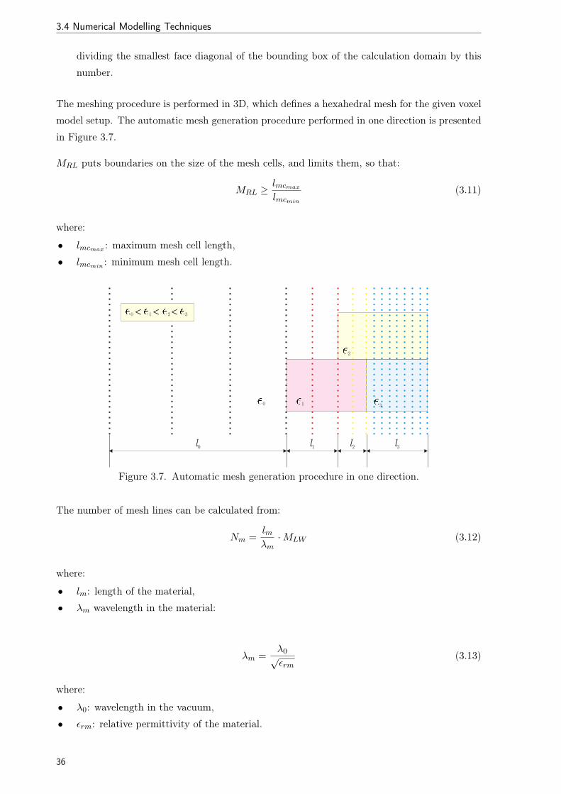
3.4 Numerical Modelling Techniques
dividing the smallest face diagonal of the bounding box of the calculation domain by this
number.
The meshing procedure is performed in 3D, which defines a hexahedral mesh for the given voxel
model setup. The automatic mesh generation procedure performed in one direction is presented
in Figure 3.7.
MRL puts boundaries on the size of the mesh cells, and limits them, so that:
MRL ≥lmcmax
lmcmin
(3.11)
where:
• lmcmax : maximum mesh cell length,
• lmcmin : minimum mesh cell length.
Figure 3.7. Automatic mesh generation procedure in one direction.
The number of mesh lines can be calculated from:
Nm =lmλm
·MLW (3.12)
where:
• lm: length of the material,
• λm wavelength in the material:
λm =λ0√εrm
(3.13)
where:
• λ0: wavelength in the vacuum,
• εrm: relative permittivity of the material.
36

Modelling MIMO Systems in Body Area Networks in Outdoors
This expression is only valid if MRL allows to define a detailed meshing as required for the tissue:
MRL ≥√εrm (3.14)
Otherwise, the meshing for a given tissue is performed with a lower resolution, and the global
parameter MLW is not fulfilled.
37

x

Chapter 4
Statistical Modelling of Antennas
on a Body
This chapter proposes a new statistical model to analyse wearable antennas in BANs, using
a simple theoretical approach or numerical analysis. In this chapter, a model to study the
correlation between signals captured by wearable antennas is presented as well. Moreover, the
method to include realistic body movement is introduced.
39

4.1 Concept and Scenarios
4.1. Concept and Scenarios
The importance of the statistical study of wearable antennas performance in the vicinity of the
body has been reported in [Sibi08]. Following that idea, this thesis considers the antenna as a
stochastic component of the radio channel, and studies the influence that the presence of the
body has on antennas performance. This presence leads to changes in the antenna gain pattern,
which depend on the distance to its surface.
Modelling of the antenna gain pattern in BANs has been decomposed as presented in Figure 4.1.
Figure 4.1. Statistical modelling of antennas on a body.
At the first stage, the influence of the presence of the static body (i.e., body coupling) is analysed.
In this case, due to the variance of tissues properties and various geometrical dimensions, a key
role is played by the location of the antenna on the body. This approach can be analysed via
theoretical, numerical or experimental approaches.
At the second stage, body dynamics are taken into account. The novel aspect of this thesis is
to present a very realistic model of body dynamics, and the corresponding influence on antenna
gain pattern from a statistical viewpoint. Firstly, statistics of the variations of the normal to
the surface of an antenna located on a moving body are calculated. Then, taking the statistical
gain pattern obtained for the static body, and previously calculated variations of the antenna
orientation, the statistical gain pattern of a wearable antenna on a moving body is derived.
By using this method, it is possible to describe and include body behaviour scenarios in Radio
Channel simulators. This is of great importance, as antenna rotation has a huge impact on the
performance of the whole transmission channel. Due to the movement of the antenna located
at the BAN side of the radio link, the antenna located at the other side of the link captures
significant signal variations in the angular power profile.
40
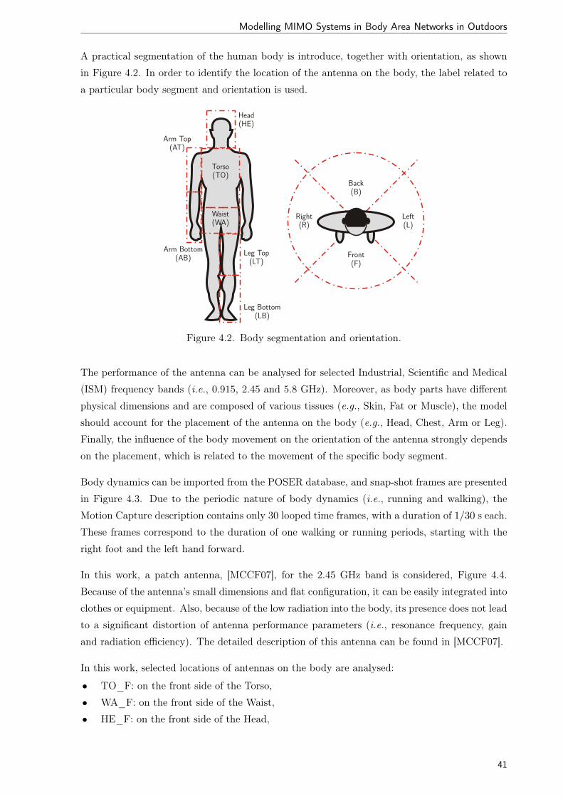
Modelling MIMO Systems in Body Area Networks in Outdoors
A practical segmentation of the human body is introduce, together with orientation, as shown
in Figure 4.2. In order to identify the location of the antenna on the body, the label related to
a particular body segment and orientation is used.
Figure 4.2. Body segmentation and orientation.
The performance of the antenna can be analysed for selected Industrial, Scientific and Medical
(ISM) frequency bands (i.e., 0.915, 2.45 and 5.8 GHz). Moreover, as body parts have different
physical dimensions and are composed of various tissues (e.g., Skin, Fat or Muscle), the model
should account for the placement of the antenna on the body (e.g., Head, Chest, Arm or Leg).
Finally, the influence of the body movement on the orientation of the antenna strongly depends
on the placement, which is related to the movement of the specific body segment.
Body dynamics can be imported from the POSER database, and snap-shot frames are presented
in Figure 4.3. Due to the periodic nature of body dynamics (i.e., running and walking), the
Motion Capture description contains only 30 looped time frames, with a duration of 1/30 s each.
These frames correspond to the duration of one walking or running periods, starting with the
right foot and the left hand forward.
In this work, a patch antenna, [MCCF07], for the 2.45 GHz band is considered, Figure 4.4.
Because of the antenna’s small dimensions and flat configuration, it can be easily integrated into
clothes or equipment. Also, because of the low radiation into the body, its presence does not lead
to a significant distortion of antenna performance parameters (i.e., resonance frequency, gain
and radiation efficiency). The detailed description of this antenna can be found in [MCCF07].
In this work, selected locations of antennas on the body are analysed:
• TO_F: on the front side of the Torso,
• WA_F: on the front side of the Waist,
• HE_F: on the front side of the Head,
41

4.1 Concept and Scenarios
(a) running body (b) walking body
Figure 4.3. Motion Capture snap-shot frames of the body movement (extracted from [POSE12]).
Figure 4.4. Patch antenna with switchable slots in a closed configuration [MCCF07].
• HE_B: on the back side of the Head,
• HE_L: on the left side of the Head,
• HE_R: on the right side of the Head,
• AB_L: on the left side of the Arm,
• AB_R: on the right side of the Arm,
• TO_B: on the back side of the Torso,
• LT_L: on the left side of the Leg,
• LT_R: on the right side of the Leg.
In case of a MIMO system with 2 wearable antennas, the correlation depends on the mutual loca-
tion of the antennas (i.e., Front, Back, Left and Right), the statistical analysis being performed
for the following classes:
• Co-Directed (CD): both antennas are located on the same side.
42

Modelling MIMO Systems in Body Area Networks in Outdoors
• Cross-Directed (XD): one antenna is located on the Back or on the Front, whereas the other
one is placed on the Left or Right.
• Opposite-Directed (OD): one antenna is located on the Back and the other on the Front,
or one antenna is located on the Left and the other on the Right.
In case of a MIMO system with more than 2 antennas, classes considering the total number of
sides covered (i.e., from 1 to 4), and a subclass label, including combinations of those sides, are
proposed in Table 4.1.
Table 4.1. Possible classes of wearable antennas in MIMO system.
number of the sides subclass labels
1 F, B, L, R
2 FB, FL, FR, BL, BR, LR
3 FBL, FBR, FLR, BLR
4 FBLR
4.2. Theoretical Model
Since the radiated far field of an antenna in the vicinity of the body is a combination of direct and
reflected fields, the influence of the body on the radiation pattern of the electric field strongly
depends on the distance of the antenna to the body. A very simple model is taken as a first
approach to the more realistic, but also more complex, problem.
In order to compute the statistical behaviour of an antenna near the body, a very simple model
based on image theory is introduced. Since the model is based on geometry, calculations are very
fast compared to full wave methods. But this modelling approach does not reproduce all the
phenomena that are caused by the presence of the body (i.e., reduction of antenna efficiency,
and mutual coupling between antenna and the body). Also, in reality, the size of the body
cannot be considered much larger than the wavelength for 0.915, 2.45 and even 5.8 GHz, so the
model can be considered just as a first approximation. This simple approach has been chosen
because of its low computational complexity, and in order to have a glimpse of the possible range
of changes in the radiation pattern of the electric field of the antenna placed in the vicinity of
the body.
Firstly, the wave reflection by an infinite plane half space is being analysed, Figure 4.5, for an
antenna at a height h from the plane.
The reflection coefficient for reflected component for perpendicular and parallel polarisations
are calculated according to (2.29) and (2.30), respectively.
In order to model various antenna positions on several locations on the body, a simple geometrical
approach has been considered. The infinite plane half space is replaced by an elliptical shaped
medium, which dimensions (i.e., am minor and aM major axes) depend on the corresponding
part of the body, Figure 4.6.
43

4.2 Theoretical Model
Figure 4.5. Model for the estimation of the radiation pattern of the electric field of an antenna
located over infinite lossy dielectric half space.
Figure 4.6. Simple model for the estimation of the radiation pattern of the electric field of an
antenna located in the vicinity of a body.
In this case, the angle of incidence θi is no longer equal to the radiation angle θ, depending also
on the distance between the antenna and the ellipse. The angle θi for a given θ, h, am and
aM , can be found from geometrical considerations. In case θ is larger than the shadowing angle
θmax, the antenna does not radiate directly in this direction, and its electric field is E(θ, ϕ) = 0.
Otherwise, the total field in the far-field is the result of the sum between the direct component
Ed, and the reflected one, Er. The total field above the body tissue can be written as:
E(θ, ϕ, h) = Ed(θ, ϕ) + Er(θ, ϕ, h)Γ(θ, ϕ, h) ej2πλ
∆d (4.1)
where:
• ∆d = dr − dd
• dr and dd are the path lengths of the reflected and direct components, respectively.
The magnitude of the electric field is given by:
44

Modelling MIMO Systems in Body Area Networks in Outdoors
|E(θ, ϕ, h)| =√|Ed|2 + |Er|2 |Γ|2 + 2 |Ed| |Er| (Γr cos (
2πλ
∆d)− Γi sin (2πλ
∆d))(4.2)
where:
• Γr = Re {Γ}• Γi = Im {Γ}
In the practical scenario of a BAN, the distance of the antenna to the body can vary in time,
which can be described statistically by a Probability Density Function (PDF), p(h). In this
case, the average value |E(θ)| for the radiation pattern of the electric field magnitude and its
standard deviation σ|E|(θ) can be obtained from:
|E(θ, ϕ)| =∞∫0
|E(θ, ϕ, h)| p(h)dh (4.3)
σ|E|(θ, ϕ) =
∞∫0
√(|E(θ, ϕ, h)| − |E(θ, ϕ)|
)2p(h)dh (4.4)
4.3. Numerical Model
In this section, by using numerical model, the statistical behaviour of the radiation pattern
of an antenna located over various parts of the body is investigated, Figure 4.7. Contrary to
theoretical approach, full wave simulations can reproduce, with high accuracy, the phenomena
that are caused by the presence of the body (i.e., mutual coupling between antenna and the
body, body shadowing, and reduction of antenna efficiency).
Figure 4.7. Numerical model for an antenna placed near the head (voxel head extracted from
[Chri10]).
When an antenna is located on the body, its performance parameters are modified by the
presence of the tissues, and the amount of change depends on the distance to the surface. In the
practical scenario for a BAN, the distance of the antenna to the body can vary in time, which can
be described statistically. Various possible distance distributions can be analysed, e.g., Uniform
or ”locally” Rayleigh. The Uniform Distribution models the possible range of changes of radiation
45

4.3 Numerical Model
pattern within the distance interval, limited by the maximum realistic distance of antenna to the
body (e.g., wearable antenna placed on a coat). The Rayleigh Distribution describes a realistic
scenario in BANs, where the distribution parameters are defined by the features of the antenna
location on the clothe: goes from 0 to a large value, and it is concentrated on a central distance.
In general, the average and standard deviation of the gain pattern, for an antenna placed on the
body, can be calculated depending on:
• distribution of the distance between antenna and body surface (e.g., Uniform or Rayleigh),
• antenna types (e.g., patch),
• antenna placements (e.g., Head, Chest, Arm or Leg),
• body types (i.e., gender, age, frame dimensions weight and height).
One of the possible tools is CST [CST12], which is a full wave simulation software, described
in detail in Section 3.4. In order to model body influence, the voxel model provided by Virtual
Family [Chri10] is used, which is presented in Section 3.2. Furthermore, in order to reduce the
calculation domain (i.e., speed up the simulations), the voxel model can be sliced into several
parts. For example, the analysis of the performance of an antenna placed on the head does not
require to model the whole body, as other fragments of the body (i.e., chest, arms, and legs)
have little influence on the gain pattern. It is recommended to use at least 4 body segments, for
the respective antenna placement, as presented in Table 4.2.
Table 4.2. Considered voxel model segments for respective antenna placements.
voxel model segment antenna placement
Head HE_F, HE_B, HE_L, HE_R
Chest TO_F, TO_B, WA_F
Arm AB_L, AB_R
Leg LT_L, LT_R
The electric parameters of the tissues (i.e., conductivity and relative permittivity) are obtained
from the 4-Cole-Cole Model [Gabr96], described in Section 3.2. It is worthwhile to notice that
this study can be performed using another full wave simulator and voxel model.
By performing simulations of the antenna located with different distances from the body hq
(a discretisation of the distance is considered, in terms of index q), one obtains a set of gain
patterns G(θn, ϕm, hq) (θn and ϕm being discrete values of the usual spherical coordinates).
The distance sample hq depends on the distribution of the distance to body, and on the total
number of distance samples Nh (i.e., the accuracy of the study). From the set of simulated gain
patterns, it is possible to calculate the average one:
Gµ(θn, ϕm) =1Nh
Nh∑q=1
G(θn, ϕm, hq) (4.5)
where:
46

Modelling MIMO Systems in Body Area Networks in Outdoors
• hq: is the qth distance sample,
• Nh: is the total number of distance samples,
• θn: is the azimuth angle sample,
• ϕm: is the elevation angle sample.
The standard deviation of the gain pattern can be calculated from:
σG(θn, ϕm) =
√√√√ 1Nh
Nh∑q=1
(G(θn, ϕm, hq)−Gµ(θn, ϕm))2 (4.6)
The average and the standard deviation of the gain pattern should be used in Radio Channel
simulators to calculate multipath components, therefore, being used as linear quantities. Howe-
ver, usually, results for an antenna’s gain pattern are shown in a logarithmic scale, hence, the
above mentioned entities are presented in dB. In this work, the following convention is used:
Gµ±σ(θn, ϕm)[dBi] = 10 log(Gµ(θn, ϕm)± σG(θn, ϕm)) (4.7)
σG(θn, ϕm)[dB] = 10 log(σG(θn, ϕm)) (4.8)
The minimum, Gmin, and maximum, Gmax, of the gain pattern are calculated from the set of
distance samples:
Gmin(θn, ϕm)[dBi] = 10 log(minhq
{G(θn, ϕm, hq)}) (4.9)
Gmax(θn, ϕm)[dBi] = 10 log(maxhq
{G(θn, ϕm, hq)}) (4.10)
The antenna gain in the direction of maximum radiation is defined as:
G0 = max {G(θ, ϕ)} (4.11)
The radiation efficiency is related to the antenna gain by:
ηa =G0
D0(4.12)
where:
• D0: is antenna directivity in the direction of maximum radiation.
In order to evaluate the difference between a general gain pattern G and a reference one Gref(e.g., the gain pattern of the isolated antenna), first the partial pattern difference, calculated
for a particular direction of radiation, can be calculated:
∆Gnm =|G(θn, ϕm)−Gref (θn, ϕm)|
Gref (θn, ϕm)(4.13)
47

4.3 Numerical Model
In general, two parameters are defined, i.e., the Pattern Average Difference (PAD):
∆G =1
NϕNθ
Nϕ∑n=1
Nθ∑m=1
∆Gnm (4.14)
and the Pattern Weighted Difference (PWD):
∆Gw =
Nϕ∑n=1
Nθ∑m=1
∆GnmGref (θn, ϕm)
Nϕ∑n=1
Nθ∑m=1
Gref (θn, ϕm)
(4.15)
where:
• Nθ: is number of discrete elevation angle samples,
• Nϕ: is number of discrete azimuth angle samples.
The difference between these two parameters is that ∆G treats changes of the gain pattern in
all directions equally, whereas ∆Gw weights these changes by the gain pattern.
As these simulations introduce discretisation errors (e.g., calculation domain meshing resolu-
tion), the influence of the simulation parameters should be evaluated, in order to achieve the
required accuracy and reasonable speed of calculations. The patch antenna has been modelled
in free space and near the voxel body model. Performing a single simulation does not provide
information about the accuracy of the solution. The FIT method guarantees that the discreti-
sation error decreases with an increasing number of mesh cells. This property can be used to
check the accuracy by refining the mesh, re-running the simulation and comparing results. It is,
however, important to find a good compromise between mesh density (affecting the simulation
time) and accuracy. Simulations were performed in a personal computer with Intel Core 2 Duo
@ 2.40 GHz processor and 3 GB of Random Access Memory (RAM). The Transient Solver was
used with an excitation signal in the band [0.3, 2.6] GHz. Table 4.3 presents the simulation time
ts and total memory Mt required for each run, which are proportional to the number of mesh
cells Nc.
Table 4.3. Complexity of selected meshing parameters scenarios.
MRL 10 7
MLW 14 12 10 16 10
Nc [106] 8.8 5.7 3.5 2.4 0.7
Mt [GB] 2.8 2.0 1.3 0.9 0.4
ts [min] 33.9 22.4 10.9 10.2 2.3
When modelling an isolated patch antenna in CST, the following parameters have been calcu-
lated:
• Gain: Ga = 6.6 dBi,
48

Modelling MIMO Systems in Body Area Networks in Outdoors
• Total radiation efficiency: ηa=80 %,
• Resonance frequency: fr = 2.44 GHz,
• Input return loss: S11 = −12.4 dB.
When comparing output parameters of the antenna in free space and near the voxel model head
for a {MLW=14, MRL=10} meshing setup, the difference in resonance frequency is 0.02 GHz.
The S11, calculated for the resonance frequency is higher (i.e., worst) by 2.0 dB when the
antenna is located near the voxel head model. The gain is reduced by -1.2 dB, and also the total
efficiency is lower by -1.0 dB (which is equal to -20%).
The input impedance (i.e., resonance frequency fr) and antenna’s radiation parameters (i.e.,
antenna gain G0, radiation efficiency ηa, gain pattern difference ∆G and ∆Gw) were analysed in
order to decide on the optimal meshing setup for simulation of the antenna in presence of the
voxel body model in CST. In Table 4.4, the results for all assessment scenarios are presented,
and the difference is calculated in reference to the {MLW=14, MRL=10} scenario.
Table 4.4. Patch antenna parameters simulated with different meshing parameters.
MRL 10 7
MLW 14 12 10 16 10
S11 [dB] -10.30 -10.43 -10.56 -11.49 -10.36
∆S11 [dB] - -0.13 -0.26 -1.19 -0.06
fr 2.460 2.462 2.455 2.455 2.492∆fr
fr[%] - 0.09 -0.19 -0.19 1.31
ηa [dB] -1.93 -1.97 -1.86 -1.86 -1.85
∆ηa [dB] - -0.04 0.07 0.07 0.08
G0 [dBi] 5.39 5.37 5.47 5.34 6.00
∆G0 [dB] - -0.02 0.08 -0.05 0.61
∆G [%] - 2.38 5.43 3.67 12.79
∆Gw[%] - 0.99 1.77 1.98 10.67
The meshing obtained for {MLW=14, MRL=10} is considered as the most accurate one, due to
the largest number of mesh cells used. The total efficiency and the gain are calculated using the
far field monitor at 2.45 GHz.
The S11 curves for all analysed meshing setups are presented in Figure 4.8. Results obtained for
all meshing setup except {MLW = 10, MRL = 7} have similar resonant frequencies, around 2.46
GHz. The magnitude of the S11 parameter is lower by 1 dB also for {MLW = 16, MRL = 7}meshing, but this parameter is not essential for the antenna gain pattern analysis, therefore
acceptable.
The changes δr of the parameters relative to the case of the maximum number of mesh cells
Ncmax (i.e., setup with {MLW=14, MRL=10}) are presented in Figure 4.9, being defined as:
δr(Nc) =|f(Nc)− f(Ncmax)|
f(Ncmax)(4.16)
49

4.4 Modelling of Signal Correlation
2.3 2.35 2.4 2.45 2.5 2.55−12
−10
−8
−6
−4
−2
0
Frequency [GHz]
S1
1 [
dB
]
LW:10 RL:10
LW:10 RL:7
LW:12 RL:10
LW:14 RL:10
LW:16 RL:7
Figure 4.8. Comparison of S11 curves for patch antenna calculated for various meshing parame-
ters.
0 1 2 3 4 5 6 7 8 90
2
4
6
8
10
12
14
16
LW:10 RL:7
LW:16 RL:7LW:10 RL:10
LW:12 RL:10
LW:14 RL:10
Number of Mesh Cells [106]
Re
lative
Diffe
ren
ce
[%
]
GainTotal EfficiencyResonance FrequencyPattern Average DifferencePattern Weighted Difference
Figure 4.9. Relative error of patch antenna parameters for various meshing scenarios.
For all meshing setups, except {MLW=10, MRL=7}, the relative error to the reference scenario
is below 5%. The meshing with {MLW=16, MRL=7} is characterised by a moderate num-
ber of mesh cells, and the results obtained from simulations are similar to meshing scenarios
{MLW=12, MRL=10} and {MLW=10, MRL=10}. Therefore, the {MLW=16, MRL=7} setup
can be considered as the optimal one in terms of complexity and accuracy.
4.4. Modelling of Signal Correlation
Many of BANs applications have extremely high safety and reliability requirements, which de-
termine the usage of multiple body-worn antennas. In BANs, multiple antennas can be placed
on various locations on the body (e.g., Head, Chest, Waist, Arm or Leg) and with various
orientations (i.e., Front, Back, Left and Right). For off-body communications, the signal is
transmitted by an external antenna, propagates in the environment, and is captured by wearable
antennas. A condition to get MIMO channel capacity gains is decorrelation between the various
MIMO links (i.e., pairs of Tx and Rx antennas). At various antennas, the received signals are
50
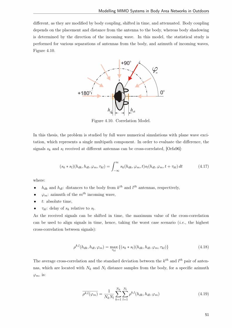
Modelling MIMO Systems in Body Area Networks in Outdoors
different, as they are modified by body coupling, shifted in time, and attenuated. Body coupling
depends on the placement and distance from the antenna to the body, whereas body shadowing
is determined by the direction of the incoming wave. In this model, the statistical study is
performed for various separations of antennas from the body, and azimuth of incoming waves,
Figure 4.10.
Figure 4.10. Correlation Model.
In this thesis, the problem is studied by full wave numerical simulations with plane wave exci-
tation, which represents a single multipath component. In order to evaluate the difference, the
signals sk and sl received at different antennas can be cross-correlated, [Orfa96]:
(sk ∗ sl)(hdk, hdl, ϕm, τkl) =∫ ∞
−∞sk(hdk, ϕm, t)sl(hdl, ϕm, t+ τkl) dt (4.17)
where:
• hdk and hdl: distances to the body from kth and lth antennas, respectively,
• ϕm: azimuth of the mth incoming wave,
• t: absolute time,
• τkl: delay of sk relative to sl.
As the received signals can be shifted in time, the maximum value of the cross-correlation
can be used to align signals in time, hence, taking the worst case scenario (i.e., the highest
cross-correlation between signals):
ρk,l(hdk, hdl, ϕm) = maxτkl
{(sk ∗ sl)(hdk, hdl, ϕm, τkl)} (4.18)
The average cross-correlation and the standard deviation between the kth and lth pair of anten-
nas, which are located with Nk and Nl distance samples from the body, for a specific azimuth
ϕm, is:
ρk,l(ϕm) =1
NkNl
Nk∑k=1
Nl∑l=1
ρk,l(hdk, hdl, ϕm) (4.19)
51

4.5 Modelling of Body Dynamics
σk,lρ (ϕm) =
√√√√ 1NkNl
Nk∑k=1
Nl∑l=1
[ρk,l(hdk, hdl, ϕm)− ρk,l(ϕm)
]2(4.20)
The average cross-correlation and the standard deviation can also be calculated as a function of
the distance of the kth antenna to the body surface, for the Nm azimuth samples:
ρk,l(hdk) =1
NlNm
Nl∑l=1
Nm∑m=1
ρk,l(hdk, hdl, ϕm) (4.21)
σk,lρ (hdk) =
√√√√ 1NlNm
Nl∑l=1
Nm∑m=1
[ρk,l(hdk, hdl, ϕm)− ρk,l(hdk)
]2(4.22)
Finally, the global average cross-correlation and the standard deviation is given by:
ρk,l =1Nm
Nm∑m=1
ρk,l(ϕm) (4.23)
σk,lρ =
√√√√ 1Nm
Nm∑m=1
ρk,l(ϕm)2
(4.24)
As the cross-correlation depends on the mutual location of the antennas (i.e., Front, Back, Left
and Right), the statistical analysis is performed for the CD, XD and OD classes. The average
and the average standard deviation can be calculated for the specific class in the usual way. It
is expected that for CD and OD antennas the average cross-correlation will be the highest and
the lowest, respectively. In the case of XD antennas, the average cross-correlation should be
moderated, however, the highest values for the standard deviation are expected.
4.5. Modelling of Body Dynamics
Capturing the movement of the body is essential for the analysis of the antenna performance.
The model for body movement is based on data taken from Motion Capture analysis. Such data
consist of a static component (i.e., skeleton hierarchy information, which is composed of several
nodes, linked to each other by a translation vector) and a dynamic one (i.e., motion data),
which is a list of rotations of the nodes for each time frame of the body movement. The node
position is calculated from the position of a previous node in the model hierarchy by solving
a forward kinematics problem [Cube06], well known from robotics. This modelling approach
can be applied to any object (e.g., human body or animal), and can describe any movement
(e.g., walking, running, jumping, crawling or dancing) in a frame-by-frame manner. One of the
52

Modelling MIMO Systems in Body Area Networks in Outdoors
data formats is Biovision Hierarchy (BVH) [DCSZ10], which is not used directly for modelling
of antenna orientation, but provides the required body movement characteristics.
In order to measure shifts of the antenna orientation, a reference coordination system has to be
selected. In this model, the reference direction is the front of the body, azimuth ϕ and elevation
ψ angles being calculated as presented in Fig. 4.11, taking the usual coordinates system.
Figure 4.11. Body directions, in the usual spherical coordinates system.
The model considers the antenna as an additional node, which is derived from the desired body
node (e.g., head, chest, hand or knee). This approach allows one not only to calculate the
position of the antenna Pa(xa, ya, za), but also to determine its normal to the body surface.
Many types of BAN antennas for off-body communications (e.g., a patch antenna [MCCF07])
have the direction of maximum radiation normal to the surface. The shifts in azimuth δϕk
and elevation δψk planes are calculated for each time frame k of the body movement. In this
case, the normal to the surface is obtained from the vector, calculated from the body node,
Pb(xb, yb, zb), to the antenna one, Pa. The spherical coordinates co-elevation θk0 and azimuth
ϕk0 of this vector have to be calculated:
θk0 = arccos(
∆zr0
)(4.25)
ϕk0 = arcsin(
∆yr0 sin(θk0)
)(4.26)
where:
• r0 =√
(∆x)2 + (∆y)2 + (∆z)2
• ∆x = xa − xb, ∆y = ya − yb, ∆z = za − zb
The shift δψk in the elevation plane is given by:
δψk = 90◦ − θk0 (4.27)
53

4.5 Modelling of Body Dynamics
whereas the shift δϕk in the azimuth plane is:
δϕk =
−180◦ − ϕk0 , ∆x < 0 and ϕk0 < 0
180◦ − ϕk0 , ∆x < 0 and ϕk0 ≥ 0
ϕk0 , other cases
(4.28)
In what follows, all output parameters are defined for the azimuth plane, however, for the
elevation one the definition is similar. Average δϕ and standard deviation σδϕ, are calculated
for all time frames:
δϕ =1NT
NT∑k=1
δϕk (4.29)
σδϕ =
√√√√ 1NT
NT∑k=1
(δϕk − δϕ
)2 (4.30)
where:
• NT : total number of time frames.
Regarding the statistics of the normal to the surface, it was found that Kumaraswamy and
Beta Distributions are the ones that best fit the selected data. These distributions can be used
for variables that are lower and upper bounded, which is the case for angles in this problem,
as the rotation of the normal to the body surface is constrained (i.e., depending on the body
movement, and antenna location). The PDF of the Beta Distribution, [MaMy78], with shape
parameters αB and βB, for the random variable δ, is:
pB(δ;αB, βB) =γαB−1B (1− γ)βB−1
B(αB, βB)(4.31)
where:
γB =δ − δmin
δmax − δmin(4.32)
• δmin and δmax: minimum and maximum shifts of the normal to the surface, respectively,
• B(αB, βB): normalisation constant to ensure that the probability integrates to unity.
The PDF of the Kumaraswamy Distribution, [Kuma80], with shape parameters αK and βK , is:
pK(δ;αK , βK) =αKβKγ
αK−1(1− γαK )βK−1
K(αK , βK)(4.33)
where:
• K(αK , βK): normalisation constant to ensure that the probability integrates to unity.
The mean calculated from simulated data δϕ can be compared to the one coming from the
Kumaraswamy Distribution EK(δϕ), for which there is a deviation defined as:
54

Modelling MIMO Systems in Body Area Networks in Outdoors
∆Kδϕ = EK(δϕ)− δϕ (4.34)
A similar parameter can be defined for the standard deviation:
∆Kσδϕ = EK(σδϕ)− σδϕ (4.35)
where:
• σδϕ: standard deviation calculated from simulated data,
• EK(σδϕ): standard deviation coming from the Kumaraswamy Distribution.
To calculate the gain pattern on a dynamic body, first, one has to obtain G(ψ,ϕ), which is an
average gain pattern for the desired placement on the static body. This average gain pattern is
calculated for an antenna which distance to the body surface is changing with a given distribution
(e.g., Rayleigh with a maximum probable distance of 2 cm); it was taken for several samples
of the distance. Instead of taking the average gain pattern, a percentile (e.g., 90th percentile)
approach can be taken for system design. Then, the gain pattern, including the shift of the
direction of maximum radiation of the antenna, is given by:
Gk(ψ,ϕ) = G(ψ + δψk, ϕ+ δϕk) (4.36)
This modelling approach still does not reproduce all the phenomena that are caused by the
presence of the moving body. The whole body moves, and when the movement of the antenna
is analysed (e.g., located on the chest), some radiation directions can be additionally obstructed
by the presence of other body segments (e.g., hands). Since the model is geometry based,
calculations are very fast compared to full wave methods. Moreover, it is very complex to
obtain realistic and dynamic body models (e.g., voxel models), which are required by full wave
modelling approaches.
From the set of previously calculated gain patterns for all time frames of body movement, it is
possible to calculate the average gain pattern:
Gµ(ψ,ϕ) =1NT
NT∑k=1
Gk(ψ,ϕ) (4.37)
and the standard deviation:
σG(ψ,ϕ) =
√√√√ 1NT
NT∑k=1
[Gk(ψ,ϕ)−Gµ(ψ,ϕ)]2 (4.38)
55

x

Chapter 5
Results of Statistical Behaviour of
Antennas on a Body
In this chapter, the results obtained from the developed models, accounting for the body coupling
(using theoretical, numerical and practical approaches) are presented and analysed. Moreover,
the statistics of the antenna gain patterns on the moving body are obtained.
57

5.1 Theoretical Approach
5.1. Body Coupling
5.1.1. Theoretical Approach
Simulations were performed for the scenarios described in Table 5.1, and always only one group of
parameters were changed while the other two were set as the Reference Scenario. The radiation
pattern of the electric field of the antenna near the body for both parallel and perpendicular
polarisations were calculated for 3 frequency bands (i.e., 915 MHz, 2.45 GHz and 5.8 GHz), 4
different body tissues (i.e., Fat, Muscle, Wet Skin and 2/3 Muscle and 1/3 Fat equivalent model)
and 3 different positions (i.e., Torso, Head and Arm). The Uniform Distribution in the range
[0, 10] cm and Rayleigh Distribution with mode 2 cm antenna to body distance were used to
calculate statistics of the radiation pattern of the electric field for all scenarios. The dimensions
of the ellipse (i.e., am and aM ) corresponding to particular body parts were set as shown in
Table 5.1, [HeUl09].
Table 5.1. Scenarios for the theoretical approach.
Scenarios Frequency [GHz] Tissue Position (aM , am) [cm]
Reference 2.45 2/3 Muscle Torso (40, 10)
Other 0.915 Fat Head (15, 15)5.8 Muscle Arm (5, 5)
Wet Skin
Figure 5.1 shows the radiation pattern of the electric field for the antenna located over an infinite
plane half space, for {0, 2.5, 5, 7.5, 10} cm. A large variation in the radiation pattern, reaching
15 dB, can be observed when the distance of the antenna to the plane is changed only by 10 cm.
As expected, an increasing distance results in a higher number of minima and maxima in the
radiation pattern of the electric field.
−20 dBi
−10 dBi
0 dBi
+10 dBi
−30 dBi
60o
o
30o
0o
−30o
−60o
o
−90o
90o
h=0 cm
h=2.5 cm
h=5 cm
h=7.5 cm
h=10 cm
Figure 5.1. The radiation pattern of the normalized electric field of an antenna located over an
infinite half space, for electric properties set to the values of the 2/3 Muscle Model, 2.45 GHz,
and parallel polarisation.
Examples of average radiation pattern of the electric field and its standard deviation for parallel
polarisation, for 915 MHz, for Uniform and Rayleigh Distributions are presented in Figure 5.2.
58

Modelling MIMO Systems in Body Area Networks in Outdoors
As Rayleigh Distribution has its mode for h = 2 cm, and decays fast with the increase of
the distance, the maximum and minimum values of the radiation pattern were calculated for
h ∈ [0, 10] cm. For θ smaller than 75◦, the average radiation pattern for the Uniform Distribution
|EU | is greater than the one for the Rayleigh distribution |ER|, and for higher θ they are the
same, rising up to 2 for 90◦. Also for angles smaller than 75◦, the maximum average radiation
pattern for |EU | is equal to 1.2 and only 0.8 for |ER|. For angles up to 80◦, |ER| is below 1,
which means a dominant destructive interference between direct and reflected components. In
the case of the antenna located over half space, the shape of the radiation pattern strongly
depends on the distance between antenna and body.
0 10 20 30 40 50 60 70 80 900
0.2
0.4
0.6
0.8
1
1.2
1.4
1.6
1.8
2
θ [o]
|E| [V
/m]
av. Uniform [0, 10] cmav. Uniform + STDav. Rayleigh (av. 2 cm)av. Rayleigh + STDmaximumminimum
Figure 5.2. The average radiation pattern of electric field of antenna located over infinite half
space, for electric properties set to the values of the 2/3 Muscle Model, for 915 MHz, for parallel
polarisation.
The full set of statistical values of radiation pattern of the electric field (i.e., the average
|EU | and the standard deviation σ|EU | for the Uniform Distribution, the average |ER| and
the standard deviation σ|ER| for the Rayleigh Distribution, |Emax| maximum, and |Emin|minimum) for both parallel and perpendicular polarisations, for selected angles of radiation
{0◦, 15◦, 30◦, 45◦, 60◦, 75◦, 90◦}, for the Reference Scenario, are gathered in Table 5.2.
For θ = 0◦, all results for both parallel and perpendicular polarisations are the same (i.e.,
Γ‖ = Γ⊥). The range of changes in the radiation pattern of the electric field is very high
(i.e., from 0 to 1.9) and depends on the angle of incidence. The average radiation pattern and
standard deviation depend on the antenna behaviour as well as polarisation. σ|ER| is always less
than σ|EU | due to the fact that, in the Uniform Distribution, the antenna is changing position
with the same probability whereas in Rayleigh Distribution distance changes less. For parallel
and perpendicular polarisations, the maximum σ|EU | is 0.45 and 0.6, whereas the maximum
σ|ER| is 0.35 and 0.5, respectively. In both cases, the standard deviation is large compared to
the average.
59

5.1 Theoretical Approach
Table 5.2. Statistical parameters for isotropic antenna over an ellipse for the Reference Scenario.
|E| , σ|E| [V/m] θ
0◦ 15◦ 30◦ 45◦ 60◦ 75◦ 90◦
pol. |EU | 1.24 1.21 1.12 1.03 1.10 1.12 0.99‖ σ|EU | 0.44 0.45 0.44 0.44 0.39 0.33 0.19
|ER| 1.44 1.40 1.32 1.19 0.99 0.80 0.87σ|ER| 0.30 0.31 0.33 0.36 0.33 0.17 0.13|Emin| 0.28 0.40 0.30 0.36 0.42 0.65 0.77|Emax| 1.72 1.71 1.68 1.65 1.57 1.51 1.57
pol. |EU | 1.24 1.21 1.15 1.08 1.19 1.25 0.92⊥ σ|EU | 0.44 0.46 0.47 0.51 0.52 0.58 0.57
|ER| 1.44 1.41 1.36 1.27 1.09 0.76 0.68σ|ER| 0.30 0.31 0.35 0.41 0.44 0.39 0.47|Emin| 0.28 0.39 0.26 0.25 0.19 0.10 0.01|Emax| 1.72 1.73 1.72 1.78 1.80 1.85 1.87
The maximum standard deviation is almost 0.5 for the Uniform Distribution at 0.915 and
5.8 GHz, and Rayleigh at 5.8 GHz, and equal to 0.3 for Rayleigh at 0.915 GHz, Figure 5.3. For
angles up to 60◦, the difference in σ|EU | for both frequencies is less than 0.05, whereas σ|ER| for
5.8 GHz is 0.25 higher than for 0.915 GHz for angles up to 75◦. It is worthwhile to notice that
for 5.8 GHz, for angles up to 60◦, σERis very close to σ|EU |, which can be explained by the fact
that the wavelength is comparable to the antenna movement also for the Rayleigh Distribution.
0 10 20 30 40 50 60 70 80 900
0.05
0.1
0.15
0.2
0.25
0.3
0.35
0.4
0.45
0.5
θ [o]
σ|E
|
Uniform, 915 MHzUniform, 5.8 GHzRayleigh, 915 MHzRayleigh, 5.8 GHz
Figure 5.3. Comparison of standard deviations for parallel polarisation, 915 MHz and 5.8 GHz,
2/3 Muscle tissue, and Torso position.
For the Uniform Distribution, the maximum standard deviation is almost 0.5 for Muscle and
0.25 for Fat, Figure 5.4. For θ less than Brewster’s angle for parallel polarisation, σ|EU | and
σ|ER| for Fat are two times less than for Muscle. This is because Fat has significantly lower
values of a permittivity and conductivity (i.e., it does not contain water), therefore, this type
60

Modelling MIMO Systems in Body Area Networks in Outdoors
of tissue has a weaker influence on the radiation pattern of antenna than others. The mini-
mum standard deviation for parallel polarisation is obtained always for radiation angles equal
to Brewster’s angle, which depends on the electrical properties of body tissues. For Fat and
Rayleigh Distribution, the minimum value of standard deviation is equal to 0.03 for θ = 75◦. In
this direction, the changes of the radiation pattern are minimal.
0 10 20 30 40 50 60 70 80 900
0.05
0.1
0.15
0.2
0.25
0.3
0.35
0.4
0.45
0.5
θ [o]
σ|E
|
Uniform, FatUniform, MuscleRayleigh, FatRayleigh, Muscle
Figure 5.4. Comparison of standard deviation for parallel polarisation, Fat and Muscle tissues,
2.45 GHz, and Torso position.
The maximum radiation angle strongly depends on the dimensions of the body part, and also
on the maximum distance from the antenna to the body, Figure 5.5.
−20 dBi
−10 dBi
0 dBi
+10 dBi
−30 dBi
150o
−30o
120o
−60o
90o
−90o
60o
−120o
30o
−150o
0o
180o
Torso
Head
Arm
Figure 5.5. Comparison of average radiation pattern for the Rayleigh Distribution, for various
positions on the body.
Concerning the location of the antenna over Torso, Head and Arm, the antenna is radiating up
to 110◦, 130◦ and 155◦, respectively. As it is expected, the largest maximum radiation angle
61

5.1 Numerical Approach
has been obtained for the smallest body part (i.e., Arm). For all positions on the body, the
average radiation pattern, for angles up to the maximum radiation angle, is changing from -3
dB to +3 dB, with maximum radiation for 0◦, minimum for 90◦, and sharp transition to 0 for
the maximum radiation angle.
Preliminary calculations with basic theoretical models show that the body causes important
changes in the antenna radiation pattern. Depending on the distance of the antenna to the
body, the reflected component can have a constructive or destructive effect on the total radiated
field. Also, the placement of the antenna is important, and among analysed tissues, the Muscle
has highest influence (i.e., the highest permittivity and conductivity) whereas Fat has the lowest.
This confirms the validity of the proposed concept of an antenna statistical model describing
the changes in its overall performance (e.g., radiation pattern, efficiency, and input impedance),
which can then be included in standards and Radio Channel models. In general, the standard
deviation is large, and one expects significant changes of the gain pattern of antenna, which is
radiating towards body tissues (e.g., a dipole antenna placed parallel to the body surface).
5.1.2. Numerical Approach
This section presents a statistical analysis of the several gain pattern of the patch antenna,
calculated at different distances between antenna and body. In order to speed up simulations,
the model of the 26-years female provided by Virtual Family has been sliced into 4 parts. The
following locations and antenna orientations being analysed: Head, Chest, Arm and Leg. This
model is one of the two adult voxels provided by Virtual Family, and it was selected because it
is the one that generates fewer mesh cells. It was decided to use only one voxel, because very
specific body parts are being studied and no great changes are expected between genders. To
perform a more detailed study, one should consider not only both genders, but also different
morphologies (i.e., fat, thin, tall etc.). Two distance distributions are analysed: Uniform in
range [0, 2λ] at 2.45 GHz, and Rayleigh with a mode of 2 cm. Simulations were performed
for 20 samples of the distance, which were calculated according to the distribution. The gain
patterns of the patch located near the Head for {0, 12λ, λ,
32λ, 2λ}, as well as the gain pattern
for an isolated patch are presented in Figure 5.6.
The highest variations are observed in the direction of the body and at the side lobes. For
the antenna attached to the Head (i.e., h = 0), the gain in the forward direction is the lowest,
and also for all other distances is less than the gain for the isolated antenna. To investigate
better the change in the gain pattern when the antenna is moving closer to the body, ∆Gw was
calculated relative to the isolated antenna for all analysed scenarios for the Uniform Distribution,
Figure 5.7.
For all body parts, the change of the gain pattern is the strongest when the antenna is located
at a distance h = 0. This is because the coupling between the body and antenna is the highest,
resulting in a significant reduction of antenna radiation efficiency, which affects the overall shape
62

Modelling MIMO Systems in Body Area Networks in Outdoors
−20 dBi −10 dBi 0 dBi +10 dBi −30 dBi
−150o
30o
−120o
60o
−90o
90o
−60o
120o
−30o
150o
0o
180o
Isolated Antenna
h=0
h=1/2λ
h=λ
h=3/2λ
h=2λ
Figure 5.6. Gain patterns of a patch antenna for various distances to the Head.
0 5 10 15 206
8
10
12
14
16
18
20
22
d [cm]
∆G
w
[%
]
HeadChestArmLeg
Figure 5.7. PWD for all analysed body regions for a distance range of [0, 2λ] at 2.45 GHz.
of the gain pattern. In general, moving the antenna away from the body results in a smaller
value of ∆Gw ; however, this is not a monotonous trend, especially in the case of the location on
the Chest.
The statistics of the gain pattern (i.e., Gµ, Gµ+σ, Gmin and Gmax) of the antenna located near
the Head relative to the isolated antenna are shown in Figure 5.8.
The average gain pattern strongly depends on the distribution of the distances between antenna
and body. The range of changes of the gain pattern is the highest in the backward direction
(i.e., ϕ = 180◦), being almost 8 dB. However, the changes in this direction are not important
for off-body communications.
The average gain pattern Gµ together with the standard deviation σG, for selected azimuth
angles of radiation ϕ = {0◦, 90◦, 180◦}, for all body parts is shown in Table 5.3.
63

5.1 Numerical Approach
0 20 40 60 80 100 120 140 160 180−10
−8
−6
−4
−2
0
2
4
azimuth [°]
Pa
tte
rn N
orm
alis
ed
to
Iso
late
d A
nte
nn
a [
dB
]
Average RayleighAverage Rayleigh + STDAverage UniformAverage Uniform + STDMinMax
Figure 5.8. Statistics of the gain pattern of the antenna located near the Head for Uniform and
Rayleigh Distributions relative to the gain pattern of the isolated antenna.
Table 5.3. Gµ and σG for selected ϕ and for θ = 90◦.
ϕ Head Chest Arm Leg
0◦ 6.2 6.5 6.2 6.1Uniform 90◦ -4.9 -5.5 -4.8 -5.0
Gµ[dBi] 180◦ -17.7 -22.8 -17.7 -21.40◦ 6.3 6.6 6.4 6.2
Rayleigh 90◦ -5.6 -6.6 -6.1 -5.7180◦ -19.2 -21.8 -16.6 -21.3
0◦ -6.1 -6.7 -4.6 -4.9Uniform 90◦ -13.9 -13.6 -12.5 -13.1
σG[dB] 180◦ -21.1 -26.1 -15.7 -24.30◦ -5.7 -7.7 -5.1 -4.2
Rayleigh 90◦ -16.5 -18.4 -13.4 -15.1180◦ -22.0 -27.4 -15.3 -23.8
The average gain pattern in the forward direction (i.e., ϕ = 0◦) varies slightly among body
regions, between 6.1 dB and 6.6 dB. Therefore, the antenna is well isolated from the body, and
changes in the antenna gain are moderated. In the backward direction (i.e., ϕ=180◦), the lowest
gain is obtained for Chest and Leg, due to the large attenuation of the body tissues. For all body
regions, the highest σG is observed for the forward direction, and for both distance distributions
for Arm and Leg, it is higher by 2 dB compared to other body regions. However, the absolute
values of the standard deviation are low, and small variations of the gain with the distance are
expected. In the backward direction, independent on the distance distribution and of the body
region, σG is very low. The reason is that in the backward direction the average gain pattern is
very low.
The comparison between average gain patterns, for the Rayleigh Distribution, for all body
regions, as well as the gain pattern of the isolated antenna are presented in Figure 5.9. Average
64

Modelling MIMO Systems in Body Area Networks in Outdoors
∆G and ∆Gw calculated relative to the isolated antenna, for all analysed locations and both
distributions, are gathered in Table 5.4.
−20 dBi −10 dBi 0 dBi +10 dBi −30 dBi
−150o
30o
−120o
60o
−90o
90o
−60o
120o
−30o
150o
0o
180o
Isolated Antenna
Head
Chest
Arm
Leg
Figure 5.9. Comparison of the average gain patterns, for the Rayleigh Distribution, and various
body regions.
Table 5.4. PAD and PWD as compared to the isolated antenna.
Head Chest Arm Leg
∆G[%] Uniform 12.1 22.2 9.7 16.0Rayleigh 18.1 24.3 18.7 22.9
∆Gw [%] Uniform 4.8 9.8 4.1 6.3Rayleigh 6.9 11.0 7.4 9.3
The relative change of the average radiation pattern for an antenna located on the Chest can
reach 24%, relative to the isolated antenna. For both distance distributions and all body regions,
∆G is higher than ∆Gw . In the case of the Uniform Distribution, when the antenna is located
with the maximum distance equal to h = 2λ (i.e., around 24.5 cm), ∆Gw and ∆G are lower
compared to the Rayleigh Distribution. This is because the influence of the body is weaker when
the antenna is moved away from the body.
The main outcome of this study are the average patterns and corresponding standard deviations.
The study is performed only for a patch antenna (i.e., which is used throughout this thesis), but
it can be easily extended to others. These results show that the patch is well isolated from the
body (i.e., similar gain for different placements and low standard deviation), which will ensure
the stability of the system.
Other results, of the statistical gain patterns obtained from this study, are gathered in Annex C.
65

5.1 Experiment
5.1.3. Experiment
The absolute gain of the antenna, G, can be measured through gain transfer techniques, using
standard gain antennas (e.g., horn antenna) [Bala05]:
G[dBi] = Gh[dBi] + 10log(PxPh
) (5.1)
where:
• Gh is the absolute gain of the horn antenna,
• Px and Ph are the received powers of the test and horn antennas, respectively.
Measurements were carried out in an anechoic chamber located at IST premises. The transmitted
power was set to 0 dBm, and the frequency to 2.45 GHz.
A calibrated horn antenna, with Gh=11.25 dBi and half power beam-width α3dB=48◦ located at
about 4 m away, was used as receiver. The patch, isolated or on the body, was the transmitter.
The system enables to sequentially retrieve the received power, the phase and the rotation angle,
generating the gain pattern. The total azimuth gain pattern is obtained from measurement of
the co- and x-polarised patterns, achieved by positioning the horn antenna in the planes θ = 0◦
and θ = 90◦.
The measurement setup is indicated in Figure 5.10. Volunteers were placed on a rotating posi-
tioner, keeping a constant velocity of 2◦/s in clockwise rotation.
Figure 5.10. Measurement setup.
Two sets of measurements were conducted: one for the isolated patch, and another for the patch
on the body. In the latter, the patch was placed at {0, 2, 4} cm (i.e., {0, 1/6λ, 1/3λ}), from the
Chest of the testers, Figure 5.11.
When measuring the isolated patch antenna, the following parameters have been obtained:
Ga=6.42 dBi; fr=2.43 GHz; S11=−14.95 dB. These values agree with the ones from literature,
[MCCF07].
66
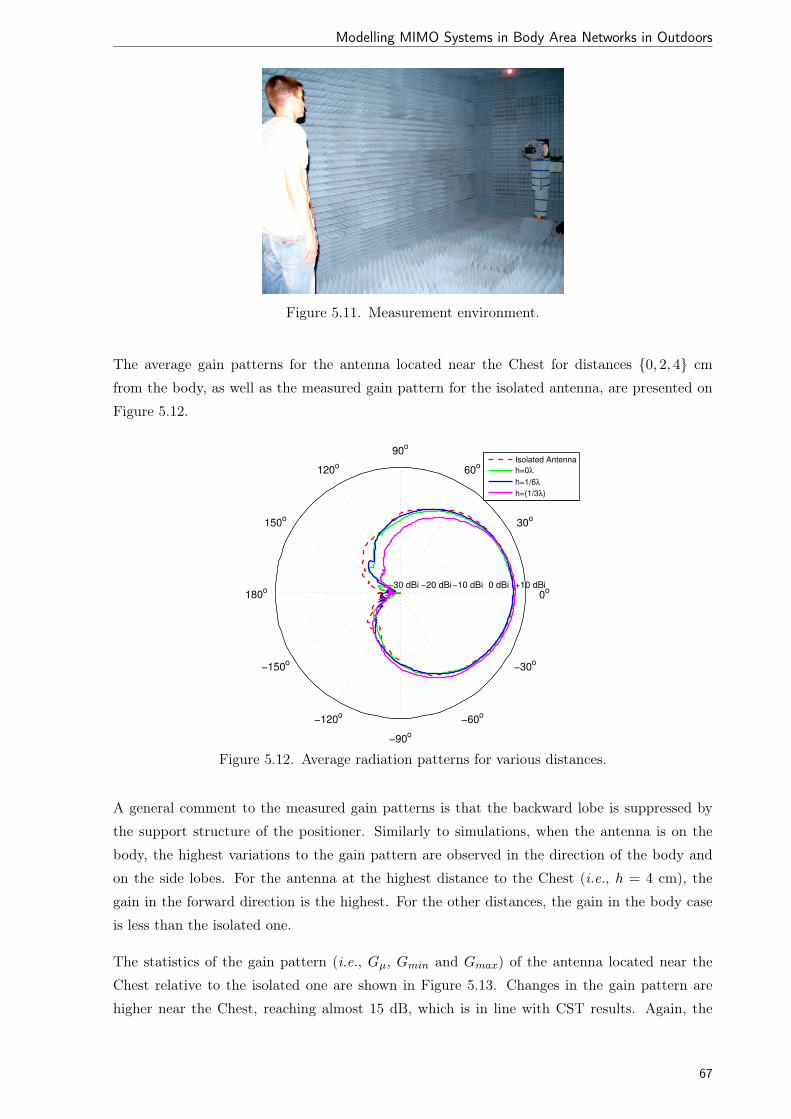
Modelling MIMO Systems in Body Area Networks in Outdoors
Figure 5.11. Measurement environment.
The average gain patterns for the antenna located near the Chest for distances {0, 2, 4} cm
from the body, as well as the measured gain pattern for the isolated antenna, are presented on
Figure 5.12.
−20 dBi −10 dBi 0 dBi +10 dBi −30 dBi
−150o
30o
−120o
60o
−90o
90o
−60o
120o
−30o
150o
0o
180o
Isolated Antenna
h=0λ
h=1/6λ
h=(1/3λ)
Figure 5.12. Average radiation patterns for various distances.
A general comment to the measured gain patterns is that the backward lobe is suppressed by
the support structure of the positioner. Similarly to simulations, when the antenna is on the
body, the highest variations to the gain pattern are observed in the direction of the body and
on the side lobes. For the antenna at the highest distance to the Chest (i.e., h = 4 cm), the
gain in the forward direction is the highest. For the other distances, the gain in the body case
is less than the isolated one.
The statistics of the gain pattern (i.e., Gµ, Gmin and Gmax) of the antenna located near the
Chest relative to the isolated one are shown in Figure 5.13. Changes in the gain pattern are
higher near the Chest, reaching almost 15 dB, which is in line with CST results. Again, the
67

5.1 Experiment
plot is not symmetric, due to the natural asymmetry of the body. The average gain pattern is
similar to the one of the isolated antenna in the range [−30◦, 30◦]. In the range [−170◦, −30◦],
the average gain pattern of the patch on the body is always below the isolated antenna one,
with a great decay on gain values for angles below −110◦. Only in backwards, it is above the
isolated patch gain pattern, with a maximum of 3 dB at −170◦, these results being influenced
by the support structure. An opposite effect is found in the symmetric range [30◦, 180◦].
−180 −90 0 90 180−15
−10
−5
0
5
10
Pat
tern
Nor
mal
ised
to Is
olat
ed A
nten
na [d
B]
azimuth [ º]
Averageminmax
Figure 5.13. Statistics of the measured gain pattern of the antenna located near the Chest,
relative to the isolated one.
Table 5.5 summarises the statistics of the measured gain pattern, averaged over the 3 sample
distances. Because of the few number of points, the interval of variations is indicated, instead
of giving the standard deviation.
Table 5.5. Gµ for selected measured ϕ and for θ = 90◦.
ϕ Isolated BodyAverage Range
0◦ 6.4 6.3 [5.7, 7.3]Gµ[dBi] 90◦ -4.7 -7.1 [-12.7, -4.0]
180◦ -22.8 -26.0 [-30.0, -22.4]
When the patch is in front of the Chest, the gain in the forward direction (i.e., ϕ = 0◦) is 0.1 dB
less than for the isolated case, with a range of changes of less than 1 dB. But, for the side lobes,
e.g., for ϕ = 90◦, differences less than 2.4 dB are found, with a higher possible range of changes.
It is worthwhile to notice that the measured bodies are different from the voxel model used in
the case of simulations.
Generally, these results are in line with the simulation ones, although in backwards there is
an obvious influence of the measurement system. Figure 5.14 confirms this, by presenting
the average gain patterns obtained through CST and measurements, for the isolated antenna
and for the antenna on the body. In the azimuth range [−90◦, 90◦], the area of interest for
68

Modelling MIMO Systems in Body Area Networks in Outdoors
off-body communications, no large changes are observed between CST and measurements: for
the isolated antenna, an average difference of 0.6 dB is found; for the antenna on the body, an
average difference of 0.9 dB is found.
−20 dBi −10 dBi 0 dBi +10 dBi −30 dBi
−150o
30o
−120o
60o
−90o
90o
−60o
120o
−30o
150o
0o
180o
Isolated CST
Isolated Measured
Body CST
Body Measured
Figure 5.14. Comparison between CST and measurements.
Although measurements deal with the whole BAN channel, they are too resource- and
time-consuming, compared to CST simulations. Moreover, when using CST it is possible to
obtain full gain patterns of antenna (i.e., in both azimuth and elevation planes). The good
agreement between measurements and simulations suggest that CST is a creditable tool to
characterise wearable antennas.
5.2. Signal Correlation
To calculate correlation, the following placements of the patch antenna, [MCCF07], are analysed:
TO_F, WA_F, HE_F, HE_B, HE_L, HE_R, AB_L, AB_R and TO_B.
Simulations were run for 11 samples of the distance, which were calculated according to the
Uniform Distribution in the range [0, 2λ] (i.e., [0, 24.5] cm). Also, a plane wave excitation has
been swept over the range [0◦, 180◦] with a resolution of 5◦ (i.e., 36 samples). This gives a total
number of 396 full wave simulations, each simulation taking about 15 minutes, using an Intel
Xeon X5600 4 × Quad-Core workstation.
Before performing the calculations of the cross-correlation, in Matlab, all signals were resampled,
in order to have the same time resolution (32 ps) and the same number of samples (250), which
corresponds to the duration of 8 ns. For all 9 considered placements of antennas, the total
number of possible pairs is equal to(92
)= 36. Therefore, for each pair of antennas, there are
69

5.2 Signal Correlation
11× 11× 36 = 4 356 possible configurations of distances and excitations. As there are 36 pairs
of antennas, a total number of 156 816 correlations were calculated.
Firstly, the average and the standard deviation of cross-correlation has been calculated for all
possible combinations of pairs of antennas. In Table 5.6, the statistics of the cross-correlation and
the allocation to the class are presented. The proposed classification of the mutual orientation
of antennas is in agreement with the obtained values of the average cross-correlation, where for
any pair of OD antennas the average cross-correlation is less than for the XD one. Also, for
the pairs of XD antennas the average cross-correlation is less than for the CD one. Due to the
similar conditions of the links, CD antennas are characterised by high values of cross-correlation,
as a result of coupling and interactions between the antenna and the body.
Table 5.6. The matrix with the definition of the classes, and simulated values of the average
and standard deviation of cross-correlation.
In Figure 5.15, the results for average cross-correlation and standard deviation are presented.
As the antennas are oriented in the same direction, the highest average cross-correlation is
obtained for the CD class, being 0.95; in this case, the standard deviation is the lowest, equal
to 0.07. This means that the signals received by the CD pair of antennas are very similar,
and correlation between them changes slightly with the azimuth of the incoming wave and the
distance from the antenna to the body. The lowest average cross-correlation is obtained for
the OD class, being 0.67, which has also a low standard deviation, equal to 0.09. In this case,
body shadowing results in significant deformation of the received signals. In the case of the
XD class, the average cross-correlation is 0.79 and the standard deviation is the largest, being
0.13, because, this class is the transition between CD and OD, which results in a high standard
deviation and a moderate average correlation. Therefore, in this case, the arriving signals can
be either low or highly correlated.
70

Modelling MIMO Systems in Body Area Networks in Outdoors
CD XD OD0.5
0.55
0.6
0.65
0.7
0.75
0.8
0.85
0.9
0.95
1
class
ave
rag
e c
orr
ela
tio
n [
ρ ]
Figure 5.15. Average and standard deviation of cross-correlation for the various classes.
The statistics of cross-correlation for a selected pair of antennas (i.e., TO_F & WA_F, HE_L
& TO_B and WA_F & HE_B), which are representative from the classes, depending on the
azimuth of the incoming wave, are presented in Figure 5.16.
0 20 40 60 80 100 120 140 160 1800.2
0.3
0.4
0.5
0.6
0.7
0.8
0.9
1
direction [°]
co
rre
latio
n
TO_F and WA_F+STD−STDHE_L and TO_B+STD−STDWA_F and HE_B+STD−STD
Figure 5.16. Average and standard deviation of cross-correlation for selected pairs of antennas.
The average cross-correlation in the pair TO_F & WA_F is very high, above 0.93, with very
small standard deviation, especially in the side direction (i.e., 90◦). In general, for the pairs of
antennas located on the same side of the body, the average cross-correlation does not depend
on the direction of the incoming wave. In case of the HE_L & TO_B pair, cross-correlation
depends on the direction, and varies a lot. The lowest values of cross-correlation are obtained in
the side and back directions, when one antenna is in LoS conditions and the other is shadowed.
For the pair WA_F & HE_B, the lowest average cross-correlation is obtained, for 170◦, and
there is also a local minimum at 10◦. In the case of 170◦, the HE_B antenna is in LoS, whereas
the WA_F one is shadowed by the torso. The attenuation and distortion caused by the head
71
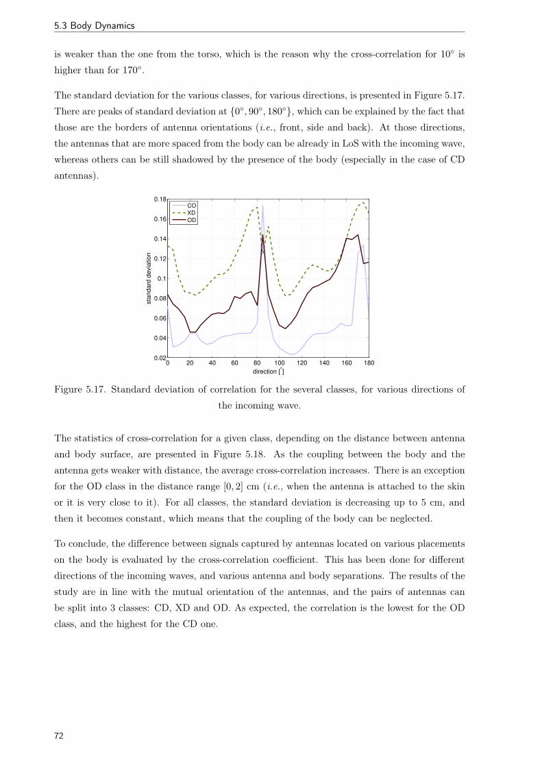
5.3 Body Dynamics
is weaker than the one from the torso, which is the reason why the cross-correlation for 10◦ is
higher than for 170◦.
The standard deviation for the various classes, for various directions, is presented in Figure 5.17.
There are peaks of standard deviation at {0◦, 90◦, 180◦}, which can be explained by the fact that
those are the borders of antenna orientations (i.e., front, side and back). At those directions,
the antennas that are more spaced from the body can be already in LoS with the incoming wave,
whereas others can be still shadowed by the presence of the body (especially in the case of CD
antennas).
0 20 40 60 80 100 120 140 160 1800.02
0.04
0.06
0.08
0.1
0.12
0.14
0.16
0.18
direction [°]
sta
ndard
devia
tion
CO
XD
OD
Figure 5.17. Standard deviation of correlation for the several classes, for various directions of
the incoming wave.
The statistics of cross-correlation for a given class, depending on the distance between antenna
and body surface, are presented in Figure 5.18. As the coupling between the body and the
antenna gets weaker with distance, the average cross-correlation increases. There is an exception
for the OD class in the distance range [0, 2] cm (i.e., when the antenna is attached to the skin
or it is very close to it). For all classes, the standard deviation is decreasing up to 5 cm, and
then it becomes constant, which means that the coupling of the body can be neglected.
To conclude, the difference between signals captured by antennas located on various placements
on the body is evaluated by the cross-correlation coefficient. This has been done for different
directions of the incoming waves, and various antenna and body separations. The results of the
study are in line with the mutual orientation of the antennas, and the pairs of antennas can
be split into 3 classes: CD, XD and OD. As expected, the correlation is the lowest for the OD
class, and the highest for the CD one.
72

Modelling MIMO Systems in Body Area Networks in Outdoors
0 50 100 150 2000.55
0.6
0.65
0.7
0.75
0.8
0.85
0.9
0.95
1
distance [mm]
co
rre
latio
n
CD AV
+STD
−STD
XD AV
+STD
−STD
OD AV
+STD
−STD
Figure 5.18. The average and standard deviation of cross-correlation for the various classes, for
several distances from the body.
5.3. Body Dynamics
The following locations of antennas on the dynamic body are being analysed: Head, Chest,
Arm and Leg. Two scenarios are analysed: the walking or running bodies, which are the most
typical human day-to-day activities, and examples of the fast and slow movement scenarios,
respectively. The statistics of changes in the direction of maximum radiation are calculated over
a single period only.
When the antenna is located on the Arm, shifts of the normal to the body surface for the running
or walking bodies are presented in Figure 5.19. When the antenna is located on the Arm, it
is expected that the change of the antenna orientation in both azimuth and elevation planes is
significant. In the azimuth plane and the running body, the direction of maximum radiation is
changing 100◦. When walking, the change of the antenna orientation is much smaller than in
the case of running.
In order to evaluate the influence of body movement on the change of the normal to the surface,
a statistical analysis was performed. The average and range of change in the antenna orienta-
tion for all analysed antenna placements, for the walking or running bodies, are presented in
Figure 5.20.
As expected, the range of changes for the running body is always larger than for the walking
one. The largest variation in antenna orientation is obtained for the Arm placement and the
running body. Considering the average direction of maximum radiation, for both movement
scenarios and respective antenna placements, results are similar and depend directly on the side
of the body (i.e., front or left). The exception is the elevation plane for the antenna located on
the Chest, which is tilted down by 10◦ for the running scenario compared to the walking one.
In this case, the body is always bent to the front.
73

5.3 Body Dynamics
0 0.2 0.4 0.6 0.8 1 1.2 1.4 1.6 1.80
20
40
60
80
100
120
140
160
time [s]
an
gle
of
rad
iatio
n [
°]
walk azimuthwalk elevationrun azimuthrun elevation
Figure 5.19. The normal to the body surface of a wearable antenna placed on the Arm, for the
walking or running bodies.
Head Chest Arm Leg
0
50
100
150
WalkRun
azim
uth
[°]
Head Chest Arm Leg
−10
0
10
20
30
40
50
ele
vation [
°]
(a) azimuth plane (δϕ) (b) elevation plane (δψ)
Figure 5.20. Average and range of change in the normal to the body surface of a wearable
antenna for the walking or running bodies.
The standard deviation of the change in the normal direction to the body surface is presented
in Figure 5.21. The placement of the antenna on the Arm when running results in the highest
standard deviation, which is 37◦ and 19◦ for azimuth and elevation angles, respectively. For
all antenna placements and walking, the standard deviation is below 4◦, which is very small
compared with the typical 3 dB beam width of antennas used in BANs. Also for the walking
body, the standard deviation for the Arm placement and azimuth plane is 11 times lower than
for the running one. Therefore, it is expected that the walking body will have not significant
impact on the gain pattern changes of wearable antennas. The Chest antenna location and
running body results in a significant standard deviation in the azimuth plane of almost 13◦, and
some changes in the gain pattern are expected. For both movement scenarios, the most stable
placement for the antenna is the Head, where the standard deviation in both planes is below 2◦.
The antenna orientation data obtained from motion capture analysis have been interpolated (by
an interpolation factor of 5), which is a good approximation, as the body moves in a smooth way.
By analysing all histograms, it has been found that they are J-shaped in most cases, however,
in some cases they are concentrated around the mean value. The Beta and Kumaraswamy
74

Modelling MIMO Systems in Body Area Networks in Outdoors
Head Chest Arm Leg 0
10
20
30
40
azim
uth
[°]
walkrun
Head Chest Arm Leg 0
5
10
15
20
ele
va
tio
n [
°]
walkrun
(a) azimuth plane (σδϕ) (b) elevation plane (σδψ)
Figure 5.21. Standard deviation of change in normal to the body surface for walking and running
bodies.
distributions have been used to fit the data. The example of the distribution of the normal to
the body surface, for the running body and Arm placement is presented in Figure 5.22.
52.5 78.4 104.3 130.3 156.20
5
10
15
20
25
30
35
40
Angle
# O
ccu
rre
nce
s
αK=0.03 β
K=0.42 χ
K
2=5.7
αB=0.29 β
B=0.49 χ
B
2=6.4
84.1 85.8 87.5 89.2 90.90
5
10
15
20
25
30
35
Angle
# O
ccu
rre
nce
sα
K=8.01 β
K=8.07 χ
K
2=58.8
αB=1.57 β
B=1.23 χ
B
2=63.7
(a) Arm location (b) Head location
Figure 5.22. Histograms and distribution fitting of the normal direction to the body surface for
the running body in the azimuth plane.
Goodness of fit has been analysed by the chi-square (χ2B and χ2
K) test, [GrNi96], and evaluation
of the correlation between the simulation data and their estimates (ρB and ρK), Table 5.7.
On average, the Kumaraswamy Distribution fits better than the Beta one (lower χ2 error and
higher correlation). In the majority of the cases, both functions give the χ2 value lower than the
threshold χ295%=18.31 for a 95% confidence interval, which means that the fitting is successful.
In this case, the shape parameters have values as follows, αk ∈ [0.01, 0.53] and βk ∈ [0.24, 0.81].
For the other cases, the deviation in mean (i.e., ∆Kδψ and ∆Kδϕ) and standard deviation
(i.e., ∆Kσδψ and ∆Kσδϕ) is not more than 1.2◦ and 1.8◦, respectively, Table 5.8. These values
are small compared with the typical 3 dB beam width of antennas used in BANs, thus, being
acceptable. In general, the fitting with the Kumaraswamy Distribution is considered successful
and sufficient.
75

5.3 Body Dynamics
Table 5.7. Measures of goodness of fit for Beta and Kumaraswamy distributions (χ295%=18.31)
and estimated shape parameters for Kumaraswamy distribution.
χ2B χ2
K ρB ρK αK βK
Run Hand ϕ 6.4 5.7 0.96 0.96 0.03 0.42θ 6.7 6.9 0.96 0.96 0.01 0.45
Chest ϕ 4.5 4.8 0.97 0.97 0.07 0.24θ 87.8 89.3 0.64 0.64 0.54 0.86
Head ϕ 63.7 58.8 0.31 0.88 8.01 8.07θ 31.4 32.7 0.79 0.78 1.67 3.43
Leg ϕ 124.5 39.9 0.62 0.93 4.47 34.67θ 56.1 56.6 0.37 0.37 0.67 0.81
Walk Hand ϕ 16.0 16.8 0.78 0.77 0.27 0.49θ 2.4 2.4 0.98 0.98 0.17 0.30
Chest ϕ 2.1 2.1 0.99 0.99 0.01 0.37θ 13.3 13.3 0.81 0.81 0.53 0.81
Head ϕ 0.5 0.4 1.00 1.00 0.16 0.36θ 0.7 0.9 1.00 0.99 0.14 0.24
Leg ϕ 22.1 22.3 0.70 0.70 0.51 0.74θ 31.1 31.0 0.70 0.70 0.37 0.77
Table 5.8. Deviation in mean and standard deviation between the data and the Kumaraswamy
Distribution (for unsuccessful fitting cases).
∆Kδψ, ∆Kδϕ [◦] ∆Kσδψ, ∆Kσδϕ [◦]
Run Chest θ 0.1 0.1Head ϕ -1.2 1.2
θ 0.3 0.3Leg ϕ 0.9 1.8
θ -0.2 -0.0
Walk Leg ϕ 0.1 -0.2θ 0.7 -0.1
As a study case, a patch antenna, [MCCF07], operating at the 2.45 GHz band, has been used,
placed parallel to the body. The average gain pattern of the antenna located on various positions
on a static body, which is required to calculate statistical gain patterns for the dynamic case, is
taken from the Section 5.1.2. Figure 5.23 presents the antenna gain, Gs, when located on the
static body.
Based on the statistical description of the direction of maximum radiation of the antenna, and
the gain pattern when it is located on the Arm on the static body (i.e., taken from the numerical
simulations in CST, the statistics of the gain pattern (i.e., average Gµ, standard deviation bars,
the minimum Gmin, and maximum Gmax) are presented in Figure 5.24.
Due to the huge variation of the antenna orientation for the running body and Arm placement,
the standard deviation of the gain pattern is also very high in all directions. As expected,
76

Modelling MIMO Systems in Body Area Networks in Outdoors
Figure 5.23. Placements and gains of the antenna on the static body.
−20 dBi −10 dBi 0 dBi +10 dBi −30 dBi
−150o
30o
−120o
60o
−90o
90o
−60o
120o
−30o
150o
0o
180o
Gµ
Gµ+σ
Gmin
Gmax
Figure 5.24. Statistics of the gain pattern of the patch antenna placed on the Arm for the
running body.
on average, the gain is the highest in the direction corresponding to the average shift in the
normal direction to the body surface for the particular antenna placement. Table 5.9 presents
the statistics in the direction of maximum radiation (i.e., δψ and δϕ).
Table 5.9. Gµ and σG for the direction of maximum radiation (δθ, δϕ).
Head Chest Arm Leg
Gµ[dBi] Static 6.3 6.6 6.4 6.2Walk 6.3 6.6 6.3 6.1Run 6.3 6.3 4.0 6.1
σG[dB] Walk -18.2 -21.3 -14.7 -15.8Run -16.4 -7.7 -0.4 -13.3
σGnorm[dB] Walk -24.5 -27.9 -21.0 -21.9Run -22.7 -14.0 -4.4 -19.4
For the walking body, the gain in the direction of maximum radiation is similar to the static one,
ranging in [6.1, 6.6] dBi. In general, the standard deviation in this direction is below -15 dB,
77

5.3 Body Dynamics
which is more than 20 dB below the average gain. As expected, the walking body has little
impact on the gain pattern of wearable antenna. For the running body, the maximum gain for
the Arm placement is 4 dBi, which is more than 2 dB below other cases. The standard deviation
for the Arm placement is very high, being 16 dB higher than in the case of Head, which is the
most stable location for the antenna. In this case, changes introduced by running body on the
gain pattern are significant and have to considered in the whole Radio Channel.
Table 5.10 presents the statistics for selected directions of radiation, i.e., ψ=0◦ and
ϕ={0◦, 90◦, 180◦}. On average, in the body forward direction (i.e., ψ=0◦ and ϕ=0◦), the
highest gain is obtained when the antenna is placed on the Chest. In the side direction (i.e.,
ψ=0◦ and ϕ=90◦) the highest gain is for Head and Leg. For the Arm placement, the average
radiation is the highest in the backward direction (i.e., ψ=0◦ and ϕ=180◦).
Table 5.10. Gµ and σG for selected ϕ and for ψ = 0◦.
ϕ Head Chest Arm Leg
0◦ -6.3 6.5 -5.2 -4.2Walk 90◦ 6.3 -6.7 4.4 6.0
Gµ[dBi] 180◦ -5.5 -20.6 -4.6 -7.30◦ -5.5 6.0 -2.4 -6.3
Run 90◦ 6.3 -6.3 3.3 6.1180◦ -6.1 -20.9 -2.3 -5.3
0◦ -18.5 -16.6 -13.7 -11.1Walk 90◦ -18.6 -14.0 -5.0 -9.8
σG[dB] 180◦ -17.8 -28.9 -13.7 -16.60◦ -14.1 -5.8 -2.8 -12.9
Run 90◦ -15.5 -7.9 0.2 -10.6180◦ -15.9 -25.5 -2.1 -13.0
0◦ -12.2 -23.1 -8.5 -6.9Walk 90◦ -24.9 -7.3 -9.4 -15.8
σGnorm[dB] 180◦ -12.3 -8.3 -9.1 -9.30◦ -8.6 -11.8 -0.4 -6.6
Run 90◦ -21.8 -1.6 -3.1 -16.7180◦ -9.8 -4.6 0.2 -7.7
When the antenna is placed on the Head, the movement scenario almost does not change the
gain pattern. This placement of the antenna results in the lowest standard deviation in the front
and side directions. The standard deviation for both movement scenarios for the Head and Leg
is very low, below -14 dB and -10 dB, respectively. Therefore, it will have no impact on the
performance of the off-body link.
The average gain patterns for the running body and all antenna placements, for θ=0 plane, are
presented in Figure 5.25. When the antenna is located on the Chest, the highest gain is in the
front, while when it is located on the left side of the Head, Arm and Leg, the highest radiation
is in the left side direction, as expected. On average, when the antenna is located on the Head
78

Modelling MIMO Systems in Body Area Networks in Outdoors
or Leg, the gain is higher than on the Arm only for ϕ=[45◦, 150◦]. This means that the huge
variation of the antenna orientation, in the case of the Arm, results in a more uniform radiation
pattern.
−20 dBi −10 dBi 0 dBi +10 dBi −30 dBi
−150o
30o
−120o
60o
−90o
90o
−60o
120o
−30o
150o
0o
180o
Head
Chest
Arm
Leg
Figure 5.25. Comparison of average gain patterns for the running body.
The average and standard deviation of the radiation pattern, in both planes (in the antenna
coordinates, where ϕ=0 and ψ=0 correspond to the direction of maximum radiation), for the
running body and Arm placement are compared with the static one in Figure 5.26. When
the body is moving, the average radiation pattern is blurred (i.e., gets more uniform). It is
worthwhile to notice that the standard deviation is the highest on the extremes of the radiation
angles, and not in the direction of maximum radiation. The reason is that the antenna is oriented
in this direction for a short time (i.e., the radiation is maximum), and then moves away from it
(i.e., the radiation is low).
(a) static body
(b) average pattern for the running body (c) standard deviation for the running body
Figure 5.26. Antenna located on the Arm.
79

5.3 Body Dynamics
A similar scenario of moving body has been considered by importing a homogeneous surface
body model from POSER into CST. Simulations have been performed for the time snap-shots
of body posture for 15 walking frames (i.e., taking each 2 frames). The comparison of the
average gain patterns obtained from the body movement model and full wave simulations is
presented in Figure 5.27.
(a) body movement model (b) full wave simulations in CST
Figure 5.27. Average radiation pattern for the Arm placement and the walking body.
In general, the model reproduces very accurately the trace of the direction of maximum radiation
of the antenna. The difference in the shape of the radiation pattern comes from the body model
used (i.e., heterogeneous voxel model and surface model), additional body shadowing (i.e.,
which cannot be fully reproduced using the body movement model), and meshing errors from
CST (i.e., due to misalignment of the antenna structure with the mesh, which varies when the
antenna is rotated). The PWD calculated between the patterns is 20%, whereas the average
gains obtained from the body movement model and simulations in CST, are 6.3 and 6.7 dBi,
respectively. It is worthwhile to notice that, for the patch antenna modelled in CST near to
the voxel and the surface models, PWD can reach 10%, [OlMC12b]. Finally, one confirms that
body dynamics can have a significant impact on the performance of the whole off-body link,
especially for a running body and the location of the antenna on an Arm.
Other results, of the gain patterns for moving body, are gathered in Annex D.
80

Chapter 6
Channel Model
In this chapter, the developed channel model for BANs and scenarios being analysed are pre-
sented. The implementation of the simulator is presented as well, together with the assessment.
Moreover, the placement of antennas, the propagation scenario, and system parameters are
defined.
81

6.1 Concept and Parameters
6.1. Concept and Parameters
In order to model the radio link between on-body antennas and external terminal, one has to
consider the influence of the body (i.e., body coupling and body movements) and account for
propagation environment (i.e., multipath propagation). Therefore, the modelling of the off-body
Radio Channel has been separated into several steps, as presented in, Figure 6.1.
Figure 6.1. Modelling concept of off-body Radio Channel.
In a first stage, for the static body, the gain pattern of the antenna is calculated using the
numerical model, as presented in Section 4.3. The result is the statistical antenna gain pattern
on the static body, taking into account the body coupling effect. In this way, various types of
antennas, and a wide range of bodies can be modelled. Also, the modelling can be performed
for various antenna on-body placements.
In a second stage, the antenna position and orientation on the moving body are calculated, taking
realistic description from Motion Capture, as presented in Section 4.5. Although the presented
statistical gain patterns are antenna dependent, the changes in the antenna orientation are
independent from the antenna design, and the method is generally usable. By using this model,
any body movement scenario can be considered in a frame-by-frame manner.
Finally, the propagation environment is modelled using the GBSC model and the parameters
of the Radio Channel are determined. In the GBSC model, the multipath characteristic of the
Radio Channel is the result of signal bounce over numerous scatterers. The MPCs are calculated
according to the positions and orientation of the on-body antenna (taking into account the shift
of the radiation pattern), position of external antenna, and the distribution of scatterers. As the
wearable antennas can be located at different heights, the GBSC model includes a 3D description
of the environment, and shifts of the antenna orientation in the azimuth and elevation planes.
The output parameters are calculated, as presented in Section 2.3.
Therefore, a flexible and novel method to model Radio Channels in off-body communications is
proposed. Using this approach, both the temporal (i.e., delay spread) and angular (i.e., angular
82

Modelling MIMO Systems in Body Area Networks in Outdoors
spread) parameters can be characterised. Developed models and algorithms are not system
dependent, so that they can be used for other systems, and not just for the one chosen for
example.
In order to have a statistical viewpoint on the propagation conditions in the particular type
of the environment, a number of simulations, Ns, are performed (i.e., each time for randomly
generated scatterers). For each randomised environment, the body is always moving along
the same path with the desired behaviour (i.e., walking or running). Therefore, for a given
time frame tn (which always occurs for the same body posture and position in the cell), the
variations in output parameters comes from the differences in the propagation environment.
In what follows, all statistics are defined for the delay spread, however, for the other output
parameters the definition is similar. The average στ (tn) and the standard deviation σστ (tn) are
calculated by:
στ (tn) =1Ns
Ns∑s=1
στ (tn, s) (6.1)
σστ (tn) =
√√√√ 1Ns
Ns∑s=1
[στ (tn, s)− στ (tf )
]2(6.2)
Moreover, the statistics can be averaged in a required range of time frames:
∆t = tM − tm (6.3)
where tm and tM are the first and the last time frames, respectively. The average στ , the
standard deviation of the average σστ and the average standard deviation σστ are calculated by:
στ∆t =
1∆t
tM∑n=tm
στ (tn) (6.4)
σ∆tστ
=
√√√√ 1∆t
tM∑n=tm
[στ (tn)− σ∆t
τ
]2(6.5)
σστ∆t =
√√√√ 1∆t
tM∑n=tm
[σστ (tn)]2 (6.6)
It is important to note that when the body is uniformly moving along the axis, the interval of
time frames [tm, tM ] corresponds directly to a distance interval [dm, dM ].
83

6.1 Concept and Parameters
The power imbalance between received signals for the kth and lth on-body antennas, and the
external Rx antenna (i.e., P kR(tn) and P lR(tn)) is:
∆PRk,l(tn)[dB] =∣∣∣∣10 log
[P kR(tn)P lR(tn)
]∣∣∣∣ (6.7)
Envelope correlation is a measure of how much a signal in one branch behaves like another. The
correlation between received signal envelopes obtained for the kth and lth on-body antennas is:
ρk,lPR=
cov(P kR(t), P lR(t))σPk
R(t)σP lR(t)
(6.8)
where:
• cov(·): covariance function,
• σPkR(t) and σP l
R(t): standard deviations of the received signal envelopes for the kth and lth
on-body antennas, respectively.
The correlation between the CIRs obtained for the kth and lth on-body antennas, and the
external Rx antenna, (i.e., hk and hl) for each time frame is, [Orfa96]:
ρk,lCIR(tn) =cov(hk(tn), hl(tn))σhk(tn)σhl(tn)
(6.9)
where:
• σhk(tn) and σhl(tn): standard deviations of the CIR for the kth and lth on-body antennas,
respectively.
For a given pair of antennas, the percentage of time when the MIMO capacity is the best is:
CpMIMObest=
NT∑n=1
best(CpMIMO(tn))
NT· 100% (6.10)
where:
• CpMIMO(tn): the MIMO capacity, for the pth pair of antennas, for tn time frame,
• best(·): equal to 1 when CpMIMO(tn) is the highest (i.e., compared to all other antenna
pairs for tn frame), 0 otherwise.
For a given pair of antennas, the percentage of time when the MIMO capacity is the worst is:
CpMIMOworst=
NT∑n=1
worst(CpMIMO(tn))
NT· 100% (6.11)
where:
• worst(·): equal to 1 when CpMIMO(tn) is the lowest (i.e., compared to all other antenna
pairs for tn frame), 0 otherwise.
84

Modelling MIMO Systems in Body Area Networks in Outdoors
In order to deeper analyse the performance of on-body antennas, a parameter that compares
obtained values of the MIMO capacity with other ones is required. Therefore, the overall
performance of given pair of antennas can be evaluated for each time frame:
CpMIMOP(tn) =
CpMIMO(tn)−minp
{CpMIMO(tn)
}maxp
{CpMIMO(tn)
}−min
p
{CpMIMO(tn)
} (6.12)
where:
• minp
{CpMIMO(tn)
}and max
p
{CpMIMO(tn)
}: the minimum and maximum MIMO capacity
(i.e., obtained among all antenna pairs for tn frame), respectively.
6.2. Model Implementation
The model is able to simulate physical radio link between multiple on-body antennas and anten-
nas located at external position. The simulation can be performed for several time frames, for the
moving body (i.e., taking precise information of the location of antennas and their orientation).
All needed parameters describing physical conditions in an environment and the specification
of the system can be given by the user. The simulator can be run automatically many times,
which allows to average results and calculate statistics for outputs. The program is able to
cooperate with other applications and well know specialised programs, like Matlab and LaTeX.
In general, to make implementation easy, and to enable further extensions of the functionalities,
the structure of the simulator is as flexible as possible. The structure of the simulator can
be decomposed into several independent blocks: Config, Environment, Body Motion, Antenna,
GBSC Algorithm and MPC, which are governed by a Simulator Manager one, Figure 6.2.
Figure 6.2. Structure of the simulator.
The Config block is associated to input parameters, which are later used by the algorithm one,
and also determine the way that the GBSC Algorithm works. The Environment block consists of
a set of clusters and scatterers distributed within a specific region, described by their reflection
85

6.3 Model Assessment
coefficients. The Body Motion block updates the current positions of the body and calculates
position of the on-body antennas and their orientations. The Antenna block is responsible
for providing the antennas gain patterns, according to the current antennas orientations. The
GBSC Algorithm block contains the heart of the program, where the physical Radio Channel
is simulated and the output signals are calculated. This block establishes the relation between
input parameters and MPCs. In the MPC block, system parameters are taken into account and
all MPCs are exported as CIR. In order to have more control on the data flow in the simulator,
the Simulator Manager block is used.
The simulator has been programmed in object oriented C++, which allows to keep each logical
module in a different class. Configuration parameters are kept in an eXtensible Markup Lan-
guage (XML) file, and the simulator itself can be run from command lines including various
config files. More information needed to run the simulator can be found in Annex A. The
files containing antenna gain patterns, and detailed information about antennas position and
orientation (i.e., prepared according to required body movement characteristics) are prepared
by other developed programs. The detailed definition of the required file format, can be found
in Annex A. The flow of information in the simulator during one simulation is depicted in
Figure 6.3.
Figure 6.3. Data flow in the simulator.
When the configuration file is read, the environment for simulations is created. For each time
frame, the location of the antennas are updated, according to the description of the body
movement. Next, existing paths in the environment are calculated. These paths are summed up
and the system parameters are taken into account, resulting in CIR between particular pairs of
input and output antennas. The same calculations are performed for all combinations of input
and output antennas.
86

Modelling MIMO Systems in Body Area Networks in Outdoors
6.3. Model Assessment
A wideband Top Loaded Monopole (TLM) antenna is used, [RoEr12], which presents an impe-
dance matching band in [2.33, 11] GHz with respect to a reflection coefficient lower than -7 dB,
with a total efficiency on the body of 70% in [2.36, 5] GHz. The presence of a ground plane in
the antenna design makes its radiation characteristics less affected by the presence of the body.
The TLM gain pattern is presented in Figure 6.4.
Figure 6.4. TLM gain pattern at 2.45 GHz.
A walking scenario is analysed, the Motion Capture description contains only Nf=30 looped
time frames, with a duration of 1/30 s each. A room scenario has been considered, Figure 6.5.
A set of 6 clusters, of 3 scatterers each, has a Uniform Distribution in the room. The power
transmitted from the wearable antenna is 1 mW, and the isotropic Rx antenna is located on the
wall at a 1.2 m height. The body is walking on a straight line, in the middle of the room (i.e.,
y=2.5 m), in x ∈ [1, 4] m.
Figure 6.5. Indoor scenario.
When the MPCs contribution is not considered, the indoor scenario reduces to the respective
anechoic chamber one.
The measured data used for comparison with simulated results come from a real-time measure-
ment campaign, [RoEr12]. It was specifically realised to characterise off-body dynamic channels
at 2.45 GHz. The test-bed was mainly composed of a Vector Network Analyser (VNA), whose
87

6.4 Model Assessment
first port was connected to the Tx antenna, placed on a 1.2 m high mast. The second port was
connected to the on-body antennas, located on the right ear, of a male subject, acting as the
Rx. The antennas are TLM, and several walking cycles were repeated by the human subject, to
characterise the dynamic aspects of the off-body transmission channels.
The path loss is calculated as defined in (2.8). The simulations of the path loss for the anechoic
chamber scenario, for all considered antenna placements, and measured path loss for the HE_R
location, are presented in Figure 6.6.
1 2 3 4
40
45
50
55
60
65
70
75
path
loss [dB
]
x [m]
HE_R simulated
HE_R measured
AB_L simulated
TO_F simulated
Figure 6.6. Path loss for various antenna placements in an anechoic chamber scenario.
For the HE_R position, the average difference of path loss between measured and simulated data
is 7.1 dB, with a standard deviation of 1.5 dB (i.e., taking all the samples into account). This
gap can be due to differences between the measured and simulated scenario, to the movement
performed by the subject, to the micro-variation of the exact antenna position, and to the
simulated body physical characteristic (dielectric properties, shape and dimensions) that were
accounted for. Moreover, the polarisation effect is not taken into account during simulations,
where it is inherently considered while performing real measurements. However, even considering
these factors of variability, the comparison of the path loss of the simulated and measured curves
show a good agreement. On average, from simulations results it can be seen that for the TO_F
placement the path loss is 25 dB more than for other placements. In this case, the antenna gain
is very low (i.e., null radiation up to -25 dBi). In a walking period, the largest variations in the
path loss are registered for AB_L (i.e., 10 dB difference).
The simulated results for the path loss for the HE_R placement, for the indoor scenario, are
presented in Figure 6.7.
The average difference between measurements and simulations are 4.5 dB, with a standard
deviation of 0.1 dB. Both results follow the same trend of the extracted mean path loss for
simulation and measurements (i.e., the standard deviation of the difference is very low), and
the gap in the values can be due to differences in the simulated environment, node on-body
88

Modelling MIMO Systems in Body Area Networks in Outdoors
1 2 3 435
40
45
50
55
60
65
70
path
loss [dB
]
x [m]
simulated mean
measured mean
simulation example
measurement example
Figure 6.7. Path loss for the HE_R placement, for the indoor scenario.
position, movement performed and body characteristics, with respected to those accounted for
during measurements.
6.4. Scenarios
In simulations, the following placements of the patch antenna, [MCCF07], are analysed: TO_F,
WA_F, HE_F, HE_B, HE_L, HE_R, AB_L, AB_R and TO_B, Figure 6.8.
Figure 6.8. Considered antenna placements.
The statistical antenna radiation patterns, accounting for the body coupling are taken from
Section 5.1.2. It is worthwhile to notice that the Head gain pattern is considered for HE_F,
HE_B, HE_L and HE_R placements; Chest gain pattern is applied for TO_F, TO_B and
WA_F placements; Arm gain pattern is used for AB_L and AB_R. The narrowband case has
been considered, with the Rx bandwidth equal to 1 MHz, which corresponds to a time resolution
equal to 1 µs.
89

6.4 Scenarios
In this thesis, a micro-cell street scenario has been considered, Figure 6.9.
Figure 6.9. Street scenario.
A set of 10 clusters, of 3 scatterers each, has a Uniform Distribution in the half space of an
ellipsoid. The power transmitted from the wearable antenna is 0 dBm, and an isotropic Rx
antenna is located on the wall of a surrounding building at 3 m height. A noise level of -100 dBm
is considered. The body is moving (i.e., walking or running) on a straight line, in the middle
of the street (i.e., y=10 m), in x ∈ [50, 150] m. The running speed was set to 14.4 km/h, and
walking to 4.8 km/h, [KmPN96]. This corresponds to Np=25 or Np=75 periods of running and
walking, respectively. Due to the periodic nature of the body dynamics, the Motion Capture
description contains only Nf=30 looped time frames, with a duration of 1/30 s each. In order
to obtain statistical parameters, each dynamic scenario has been repeated Ns=30 times (for a
random distribution of scatterers).
The total number of obtained CIRs, for a particular antenna placement and dynamic scenario
is:
NCIR = Np ·Nf ·Ns (6.13)
Therefore, for each antenna placement, and the running and walking bodies, the total number
of performed simulations is 22 500 and 67 500, respectively. To obtain the CIRs for the more
demanding body movement (i.e., walking body), 0h30 of simulations was required (and 1h00
more to obtain the parameters and their statistics) using a laptop with a Core i5 Processor and
8Gb of RAM.
90

Chapter 7
MIMO Capacity in BANs
In this chapter, the results from simulations of the off-body channel are presented. The selection
of the best on-body placements of antennas is done, based on the values of MIMO capacity.
91

7.1 Radio Channel Parameters
7.1. Radio Channel Parameters
7.1.1. Propagation Conditions
Firstly, the propagation conditions are analysed, precisely in the case when the 3 dB beam width
of the Tx antenna is directed towards the Rx position, LoS being considered. The percentage of
LoS links for the walking or running bodies is gathered in Table 7.1.
Table 7.1. Percentage of LoS propagation for walking or running bodies.
LoS propagation [%]
HE_F AB_L AB_R TO_B
Walk 39.3 19.2 0.0 40.5
Run 38.3 26.1 0.0 39.5
The percentage of LoS cases depends mostly on the antenna placement, and the results are
similar for both movement scenarios, with the exception of the left arm (i.e., AB_L) case. In
the case of the running body, the movement of the arm is very large, and the AB_L antenna is
in LoS in 7% more time than for walking. The LoS or NLoS conditions for the running body, is
presented in Figure 7.1.
50 70 90 110 130 150NLoS
LoS
HE
_F
50 70 90 110 130 150NLoS
LoS
AB
_L
50 70 90 110 130 150NLoS
LoS
AB
_R
50 70 90 110 130 150NLoS
LoS
TO
_B
x [m]
Figure 7.1. Propagation conditions for the running body.
As the Rx is located on the left side of the body, the antenna placed on the right arm (i.e.,
AB_R) is always in NLoS. The antenna placed on the forehead (i.e., HE_F) is in LoS until
87 m, then its gain towards the Rx antenna is decreasing, and it becomes NLoS. The antenna on
the back (i.e., TO_B) is in NLoS when the body is approaching the Rx antenna, until 105 m.
As the torso during Run is waving to the left and right, in x ∈ [105, 115] m the propagation
conditions are changing, then after 115 m the TO_B antenna stays in LoS. In the case of
AB_L, the propagation conditions are changing from LoS to NLoS and vice-versa, due to the
large variation of the direction of maximum radiation of the antenna.
92
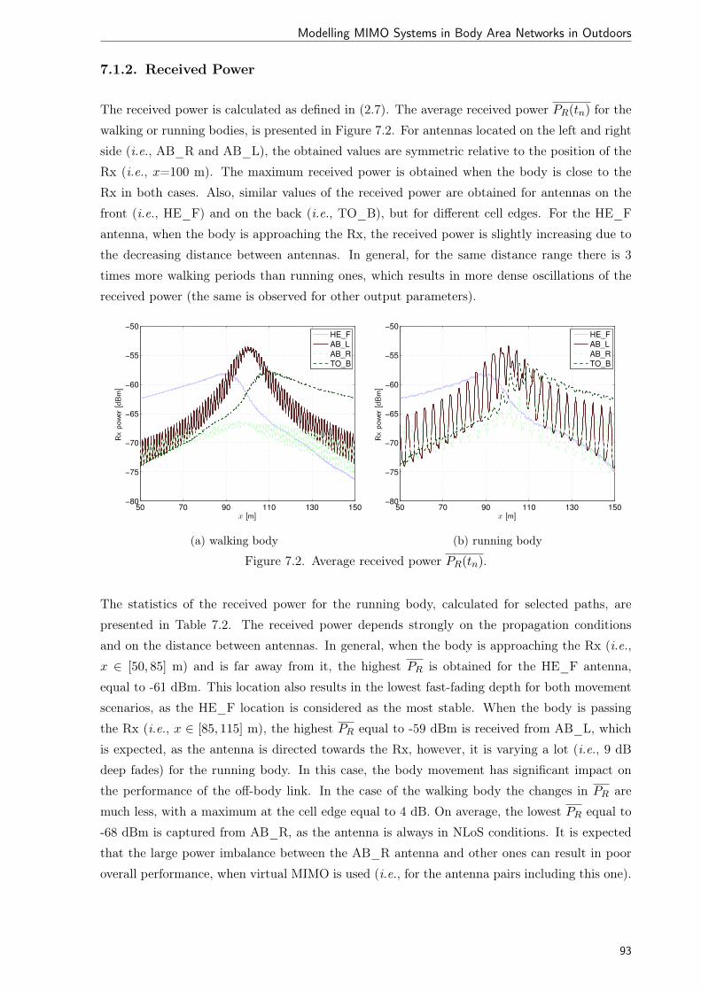
Modelling MIMO Systems in Body Area Networks in Outdoors
7.1.2. Received Power
The received power is calculated as defined in (2.7). The average received power PR(tn) for the
walking or running bodies, is presented in Figure 7.2. For antennas located on the left and right
side (i.e., AB_R and AB_L), the obtained values are symmetric relative to the position of the
Rx (i.e., x=100 m). The maximum received power is obtained when the body is close to the
Rx in both cases. Also, similar values of the received power are obtained for antennas on the
front (i.e., HE_F) and on the back (i.e., TO_B), but for different cell edges. For the HE_F
antenna, when the body is approaching the Rx, the received power is slightly increasing due to
the decreasing distance between antennas. In general, for the same distance range there is 3
times more walking periods than running ones, which results in more dense oscillations of the
received power (the same is observed for other output parameters).
50 70 90 110 130 150−80
−75
−70
−65
−60
−55
−50
x [m]
Rx
pow
er[d
Bm
]
HE_F
AB_L
AB_R
TO_B
50 70 90 110 130 150−80
−75
−70
−65
−60
−55
−50
x [m]
Rx
pow
er[d
Bm
]
HE_F
AB_L
AB_R
TO_B
(a) walking body (b) running body
Figure 7.2. Average received power PR(tn).
The statistics of the received power for the running body, calculated for selected paths, are
presented in Table 7.2. The received power depends strongly on the propagation conditions
and on the distance between antennas. In general, when the body is approaching the Rx (i.e.,
x ∈ [50, 85] m) and is far away from it, the highest PR is obtained for the HE_F antenna,
equal to -61 dBm. This location also results in the lowest fast-fading depth for both movement
scenarios, as the HE_F location is considered as the most stable. When the body is passing
the Rx (i.e., x ∈ [85, 115] m), the highest PR equal to -59 dBm is received from AB_L, which
is expected, as the antenna is directed towards the Rx, however, it is varying a lot (i.e., 9 dB
deep fades) for the running body. In this case, the body movement has significant impact on
the performance of the off-body link. In the case of the walking body the changes in PR are
much less, with a maximum at the cell edge equal to 4 dB. On average, the lowest PR equal to
-68 dBm is captured from AB_R, as the antenna is always in NLoS conditions. It is expected
that the large power imbalance between the AB_R antenna and other ones can result in poor
overall performance, when virtual MIMO is used (i.e., for the antenna pairs including this one).
93
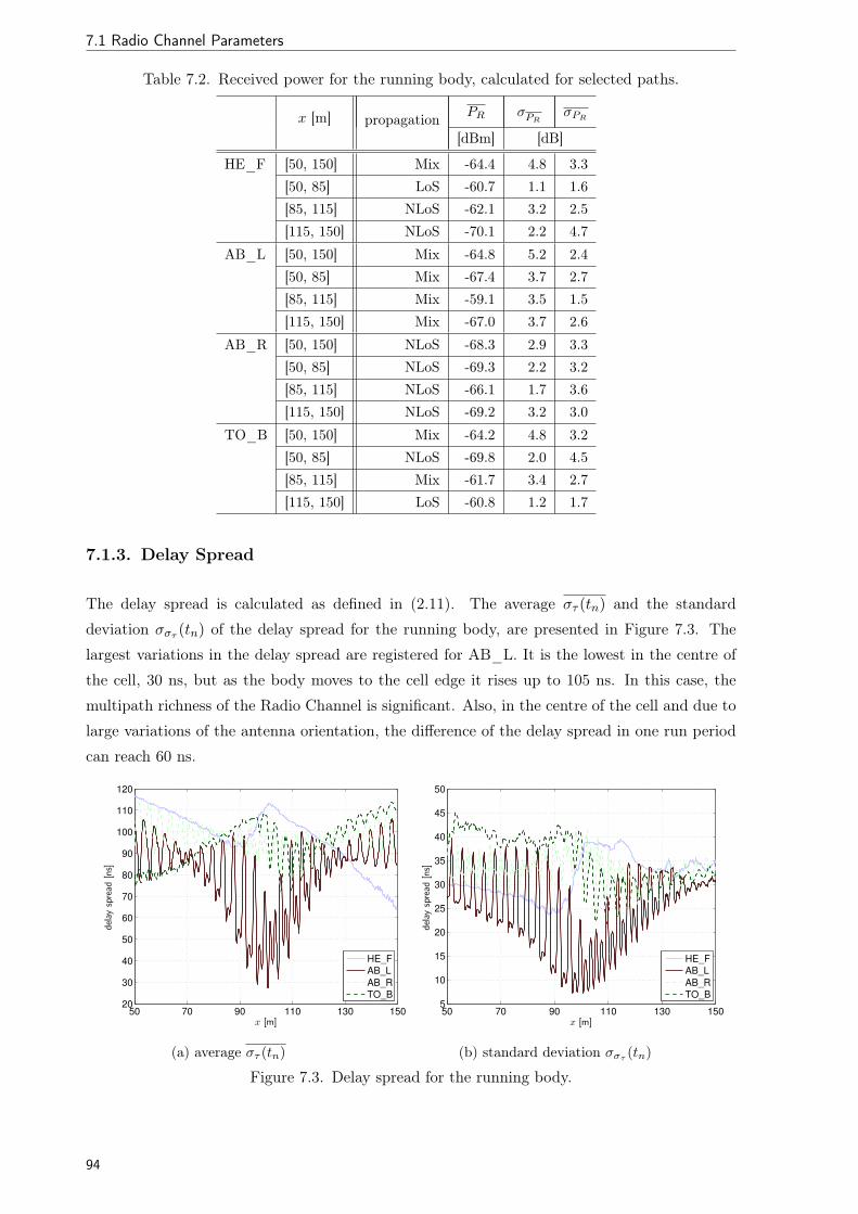
7.1 Radio Channel Parameters
Table 7.2. Received power for the running body, calculated for selected paths.
x [m] propagation PR σPRσPR
[dBm] [dB]
HE_F [50, 150] Mix -64.4 4.8 3.3[50, 85] LoS -60.7 1.1 1.6[85, 115] NLoS -62.1 3.2 2.5[115, 150] NLoS -70.1 2.2 4.7
AB_L [50, 150] Mix -64.8 5.2 2.4[50, 85] Mix -67.4 3.7 2.7[85, 115] Mix -59.1 3.5 1.5[115, 150] Mix -67.0 3.7 2.6
AB_R [50, 150] NLoS -68.3 2.9 3.3[50, 85] NLoS -69.3 2.2 3.2[85, 115] NLoS -66.1 1.7 3.6[115, 150] NLoS -69.2 3.2 3.0
TO_B [50, 150] Mix -64.2 4.8 3.2[50, 85] NLoS -69.8 2.0 4.5[85, 115] Mix -61.7 3.4 2.7[115, 150] LoS -60.8 1.2 1.7
7.1.3. Delay Spread
The delay spread is calculated as defined in (2.11). The average στ (tn) and the standard
deviation σστ (tn) of the delay spread for the running body, are presented in Figure 7.3. The
largest variations in the delay spread are registered for AB_L. It is the lowest in the centre of
the cell, 30 ns, but as the body moves to the cell edge it rises up to 105 ns. In this case, the
multipath richness of the Radio Channel is significant. Also, in the centre of the cell and due to
large variations of the antenna orientation, the difference of the delay spread in one run period
can reach 60 ns.
50 70 90 110 130 15020
30
40
50
60
70
80
90
100
110
120
x [m]
delay
spre
ad[n
s]
HE_F
AB_L
AB_R
TO_B
50 70 90 110 130 1505
10
15
20
25
30
35
40
45
50
x [m]
delay
spre
ad[n
s]
HE_F
AB_L
AB_R
TO_B
(a) average στ (tn) (b) standard deviation σστ(tn)
Figure 7.3. Delay spread for the running body.
94

Modelling MIMO Systems in Body Area Networks in Outdoors
The statistics of the delay spread for the running body, calculated for selected paths, are pre-
sented in Table 7.3. In general, στ is higher when the antenna is in NLoS or it is farther away
from the Rx. In this case, the signal is reaching the Rx antenna via reflections on the randomly
distributed scatterers, which results in larger delays of the MPCs. The highest value of σστ ,
40 ns, is obtained for the NLoS case and the TO_B antenna, when the body is in the cell edge
(i.e., x ∈ [50, 85] m). The στ for HE_F, AB_R and TO_B ranges in [87, 107] ns, with the σστ
up to 10 ns. The lowest στ , equal to 61 ns, is obtained for AB_L, when the body is close to
the Rx (i.e., x ∈ [85, 115] m), which is expected, as the LoS component is dominant (i.e., low
multipath richness of the Radio Channel).
Table 7.3. Delay spread for the running body, calculated for selected paths.
x [m] propagation στ σστσστ
[ns]
HE_F [50, 85] LoS 106.7 6.2 28.3[85, 115] NLoS 102.9 6.6 33.3
AB_L [50, 85] Mix 88.1 9.0 27.6[85, 115] Mix 61.3 18.7 18.1
AB_R [50, 85] NLoS 100.6 6.0 33.2[85, 115] NLoS 93.4 6.0 34.5
TO_B [50, 85] NLoS 86.7 6.7 40.3[85, 115] Mix 96.3 10.3 34.6
7.1.4. Spread of the Direction of Arrival
For a fixed radio link, the spatial parameters can be calculated for both ends of the radio link,
however, when the Tx antenna is located on a dynamic body, the DoD depends also on the
orientation of the on-body antenna. Therefore, in this thesis only DoA spread is calculated
as defined in (2.15). The average DoA spread σDoA(tn) for the walking body is presented in
Figure 7.4. At the centre of the cell, for the AB_L antenna the DoA spread is the lowest, 15◦
(i.e., the power of LoS component is dominant), but it increases to 45◦ in the cell edge (i.e.,
MPCs arrive from different directions). The results for HE_F and TO_B are similar for the
opposite cell edges, a small difference coming from the placement of the antenna on different
heights on the body.
The statistics of the DoA spread for the walking body, calculated for selected paths, are presented
in Table 7.4. The DoA spread increases when the antenna is in NLoS or it is farther away from
the Rx. Therefore, for all antenna placements, the σDoA is lower when the body is close to the
Rx, and it is the lowest for AB_L, equal to 20◦. This value is 2 times lower than the average
for AB_R, which is constantly in NLoS. The average of the standard deviation σσDoA is varying
in [9◦, 13◦]. Except for AB_L, the standard deviation of the average DoA σσDoA is below 6◦.
Similar results for the DoA spread have been obtained for both walking or running bodies (i.e.,
bodies were moving along the same path and had the same orientations with the Rx).
95

7.1 Radio Channel Parameters
50 70 90 110 130 15010
15
20
25
30
35
40
45
50
55
x [m]
angularsp
read
[◦]
HE_F
AB_L
AB_R
TO_B
Figure 7.4. Spread of DoA for the walking body.
Table 7.4. Spread of DoA for the walking body, calculated for selected paths.
x [m] propagation σDoA σσDoAσσDoA
[◦]
HE_F [50, 150] Mix 39.4 4.1 13.4[85, 115] NLoS 35.2 2.1 11.4
AB_L [50, 150] Mix 34.1 10.3 11.1[85, 115] Mix 20.2 4.7 9.0
AB_R [50, 150] NLoS 42.6 3.7 12.6[85, 115] NLoS 38.7 2.2 12.7
TO_B [50, 150] Mix 38.9 6.3 13.0[85, 115] Mix 33.7 2.7 11.7
The detailed information of RCPs for the street scenario is gathered in Annex E.
7.1.5. Correlation between Received Signal Envelopes
The correlation between received signal envelopes is calculated as defined in (6.8). The corre-
lation between signal envelopes has been calculated for all possible combinations of antennas,
and the statistics have been calculated for the general classes, Figure 7.5.
In general, similar results for the correlation have been obtained for both walking and running
bodies. The highest correlation is obtained, when both antennas are located on the front side,
being on average equal to 0.60 (a value of correlation being 0.70 or less can be used as the
guideline for successful diversity operation).c In this case, the running body is characterised
by slightly higher standard deviation, equal to 0.10. The largest differences between signals are
found for antennas located on the front and back sides. The average correlation is equal to -0.30,
which means that signals follow opposite trends. In this case, the envelopes of the two on-body
antennas do not exhibit the same fading behaviour, which translates into a lower probability
96

Modelling MIMO Systems in Body Area Networks in Outdoors
F B L R FL FR BL BR FB LR−1
−0.8
−0.6
−0.4
−0.2
0
0.2
0.4
0.6
0.8
1
corr
ela
tion
F B L R FL FR BL BR FB LR−1
−0.8
−0.6
−0.4
−0.2
0
0.2
0.4
0.6
0.8
1
corr
ela
tion
(a) walking body (b) running body
Figure 7.5. The correlation between received signal envelopes for the antenna class.
of having both antennas in a null at the same time. When at least one antenna is located on
the right side and is constantly in NLoS conditions (i.e., R, LR, FR or BR class), the average
correlation is very low, ranging in [0.10, 0.25]. Also, in this case the signals do not fade, peak,
increase, and decrease at the same time.
The lower the envelope correlation in a diversity system, the larger the achievable diversity
gain. Therefore, the independent fading of the signals can be obtained, by the placement of the
antennas in opposite sides of the body.
7.1.6. Correlation between Channel Impulse Responses
The correlation between CIRs is calculated as it is defined in (6.9). The average correlation
for a selected pair of antennas (i.e., TO_F & WA_F, HE_F & AB_L and HE_L & HE_R),
which are representative of various classes, is presented in Figure 7.6. In this study, in order to
obtain several incoming rays, the filtering of MPCs at the Rx with a time resolution equal to
50 ns has been considered.
For TO_F & WA_F, the correlation is high, ρCIR ∈ [0.7, 0.85], but when the body is passing
the Rx (i.e., x ∈ [100, 115] m), it drops down to 0.6. This variation occurs due to a transition
of propagation conditions from LoS to NLoS. In the case of antennas located on different sides
of the head (i.e., HE_L & HE_R), the correlation is the lowest, ρCIR ∈ [0.2, 0.45]. In this case,
the channels do not exhibit the same behaviour, which is required by the MIMO system. For
the HE_F & AB_L, when one antenna is located on the arm, and the direction of maximum
radiation is rapidly changing, the correlation is varying a lot, and a difference of 0.4 during a
single running period is registered. In the case of the walking body, the changes in correlation
are much less, with a maximum at the cell edge equal to 0.15. When the body is approaching
the Rx, the correlation is increasing and reaching its maximum when the body is close to the
Rx, then, it sharply goes down. In general, for the same distance range, there are 3 times more
walking periods than running ones, which results in more dense oscillations of the correlation.
97
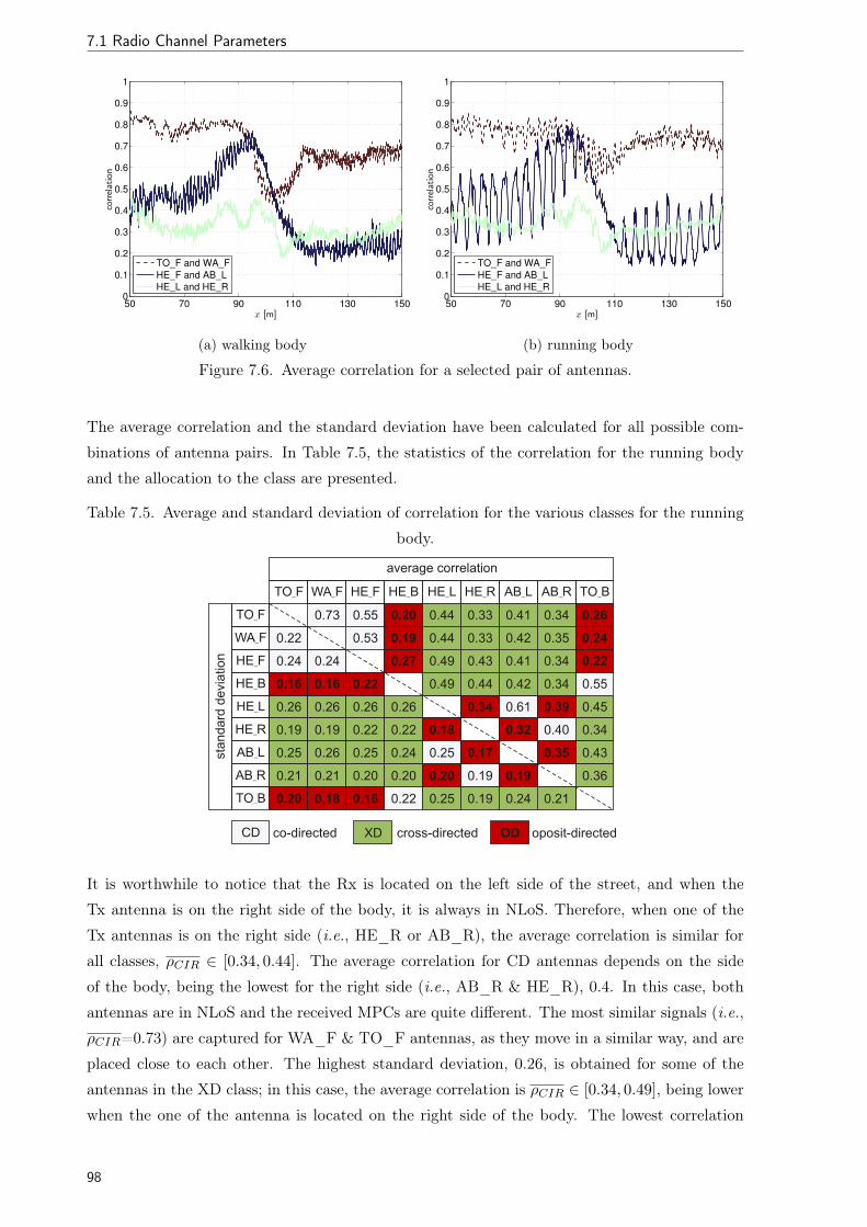
7.1 Radio Channel Parameters
50 70 90 110 130 1500
0.1
0.2
0.3
0.4
0.5
0.6
0.7
0.8
0.9
1
x [m]
correlat
ion
TO_F and WA_F
HE_F and AB_L
HE_L and HE_R
50 70 90 110 130 1500
0.1
0.2
0.3
0.4
0.5
0.6
0.7
0.8
0.9
1
x [m]
correlat
ion
TO_F and WA_F
HE_F and AB_L
HE_L and HE_R
(a) walking body (b) running body
Figure 7.6. Average correlation for a selected pair of antennas.
The average correlation and the standard deviation have been calculated for all possible com-
binations of antenna pairs. In Table 7.5, the statistics of the correlation for the running body
and the allocation to the class are presented.
Table 7.5. Average and standard deviation of correlation for the various classes for the running
body.
It is worthwhile to notice that the Rx is located on the left side of the street, and when the
Tx antenna is on the right side of the body, it is always in NLoS. Therefore, when one of the
Tx antennas is on the right side (i.e., HE_R or AB_R), the average correlation is similar for
all classes, ρCIR ∈ [0.34, 0.44]. The average correlation for CD antennas depends on the side
of the body, being the lowest for the right side (i.e., AB_R & HE_R), 0.4. In this case, both
antennas are in NLoS and the received MPCs are quite different. The most similar signals (i.e.,
ρCIR=0.73) are captured for WA_F & TO_F antennas, as they move in a similar way, and are
placed close to each other. The highest standard deviation, 0.26, is obtained for some of the
antennas in the XD class; in this case, the average correlation is ρCIR ∈ [0.34, 0.49], being lower
when the one of the antenna is located on the right side of the body. The lowest correlation
98

Modelling MIMO Systems in Body Area Networks in Outdoors
is obtained for OD antennas, in particular for HE_B & WA_F, equal to 0.19. In this case,
the gain of the MIMO system can be the highest, however, one has also consider the power
imbalance. However, in the case of antennas located on the opposite side, but on the Head, the
average correlation is higher, equal to 0.27 and 0.34, for HE_F & HE_B and HE_L & HE_R,
respectively. In this case, the antennas are placed at the same height, and with a small spacing
between them.
The statistics for CD, XD and OD antennas are presented in Table 7.6.
Table 7.6. The average and standard deviation of the correlation for CD, XD and OD antennas
for walking or running bodies.
CD XD OD
ρCIR Walk 0.56 0.39 0.27Run 0.56 0.40 0.28
σρCIRWalk 0.22 0.22 0.17Run 0.23 0.23 0.18
In general, similar results have been obtained for both walking and running bodies. The proposed
classification of the mutual orientation of antennas is in agreement with the obtained values of
the average correlation, where for OD antennas the average correlation is less than for the
XD ones. Also, for the XD antennas, the average correlation is less than for the CD ones. The
standard deviation for the walking body is less than for the running one, which can be explained
by walking being less dynamic than running, but the difference is very low. In the case of OD
antennas, the standard deviation is 0.05 less than for the two other classes (i.e., CD and XD).
7.2. MIMO Capacity
The MIMO capacity is calculated as defined in (2.19). The average capacity, the capacity
boundaries and Rx power, for the running body, for a particular pair of antennas (i.e., WA_F
& TO_B) are presented in Figure 7.7.
As the Tx antennas are located on opposite sides of the body, the Rx power is symmetric and
similar for the opposite edges of the cell. At the cell edges, the power imbalance (6.7) is high,
above 10 dB, and the capacity is close to the lower bound. The minimum power imbalance
between Tx antennas is obtained when the body is close to the Rx (i.e., x = 100 m), which
results in higher capacity (i.e., close to the upper bound). In the centre of the cell, the difference
between capacity in one running period can reach 4 bps/Hz.
The average capacity for a selected pair of antennas (i.e., TO_F & WA_F, HE_F & AB_L
and HE_L & HE_R), which are representative from various classes, is presented in Figure 7.8.
In the case of the TO_F & WA_F pair, the difference between cell edges is very high (i.e.,
20 bps/Hz on the left side and 6 bps/Hz on the right one). When the body is approaching the
99

7.2 MIMO Capacity
50 70 90 110 130 15010
12
14
16
18
20
22
24
26
28
30
capacity [bps/H
z]
x [m]
average capacity
upper bound
lower bound
50 70 90 110 130 150−115
−110
−105
−100
−95
−90
−85
Rx p
ow
er
[dB
m]
x [m]
WA_F
TO_B
(a) capacity (b) Rx power
Figure 7.7. Averages for 2×2 MIMO with WA_F & TO_B antennas, for the running body.
50 70 90 110 130 1506
8
10
12
14
16
18
20
22
24
26
ca
pa
city [
bp
s/H
z]
x [m]
TO_F and WA_F
HE_F and AB_L
HE_L and HE_R
Figure 7.8. Average capacity for selected pair of antennas from the CD, XD and OD antenna
classes, for the running body.
Rx, the capacity is increasing and reaching its maximum, 24 bps/Hz, when the body is close to
the Rx, then, it sharply goes down. For the HE_F & AB_L, when one antenna is located on
the arm, and the direction of maximum radiation is rapidly changing, the capacity is varying
a lot, and a difference of 6 bps/Hz during a single running period is registered. In the case of
antennas located on different sides of the head (i.e., HE_L & HE_R), the capacity is equal to
14 bps/Hz on both sides of the cell edges, and the maximum is obtained when the body is close
to the Rx, equal to 19.2 bps/Hz.
The statistics of the capacity and the capacity channel gain, for the same pair of antennas, for
the running body, calculated for selected paths, are presented in Table 7.7. The results for other
pair of antennas are gathered in Annex F.
In the case of CD antennas (i.e., TO_F & WA_F), the standard deviation of the average
capacity, σCMIMO, is the highest, being 6.2 bps/Hz. For all pairs of antennas, the different
100

Modelling MIMO Systems in Body Area Networks in Outdoors
Table 7.7. The capacity and the capacity channel gain, for selected pair of antennas, for the
running body, calculated for selected paths.
x [m] CMIMO σCMIMOσCMIMO
GMIMOc σGMIMOcσGMIMOc
[bps/Hz]
TO_F [50, 150] 16.41 6.23 2.21 1.45 0.17 0.17& [50, 85] 21.60 1.37 2.25 1.59 0.05 0.16
WA_F [85, 115] 19.40 4.02 2.34 1.53 0.09 0.17[115, 150] 8.78 1.77 2.06 1.26 0.08 0.18
HE_F [50, 150] 17.91 4.36 1.90 1.38 0.18 0.15& [50, 85] 19.70 2.75 2.06 1.46 0.17 0.15
AB_L [85, 115] 21.40 3.19 2.02 1.45 0.17 0.13[115, 150] 13.29 1.85 1.61 1.24 0.10 0.16
HE_L [50, 150] 16.35 1.39 1.79 1.36 0.14 0.16& [50, 85] 16.10 1.28 1.94 1.43 0.06 0.18
HE_R [85, 115] 17.59 0.95 1.72 1.17 0.06 0.12[115, 150] 15.67 1.13 1.71 1.47 0.07 0.17
location of the scatterers results in the average standard deviation of the capacity, σCMIMO,
ranging in [1.7, 2.3] bps/Hz. The average capacity channel gain, GMIMOc , for the whole distance
range (i.e., x ∈ [50, 150] m) is in [1.36, 1.46], whereas, the standard deviation of the average
capacity channel gain, σGMIMOc, and the average standard deviation of the capacity channel
gain, σGMIMOc, is below 0.2.
The average capacity and the standard deviation have been calculated for all possible combina-
tions of antenna pairs. In Figure 7.9, the statistics of the capacity for the running body and the
allocation to the class are presented.
10
15
20
25
TO
_F
& W
A_F
TO
_F
& H
E_F
WA
_F
& H
E_F
HE
_B
& T
O_B
HE
_L &
AB
_L
HE
_R
& A
B_R
TO
_F
& H
E_L
TO
_F
& A
B_L
WA
_F
& H
E_L
WA
_F
& A
B_L
HE
_F
& H
E_L
HE
_F
& A
B_L
TO
_F
& H
E_R
TO
_F
& A
B_R
WA
_F
& H
E_R
WA
_F
& A
B_R
HE
_F
& H
E_R
HE
_F
& A
B_R
HE
_B
& H
E_L
HE
_B
& A
B_L
HE
_L &
TO
_B
AB
_L &
TO
_B
HE
_B
& H
E_R
HE
_B
& A
B_R
HE
_R
& T
O_B
AB
_R
& T
O_B
TO
_F
& H
E_B
TO
_F
& T
O_B
WA
_F
& H
E_B
WA
_F
& T
O_B
HE
_F
& H
E_B
HE
_F
& T
O_B
HE
_L &
HE
_R
HE
_L &
AB
_R
HE
_R
& A
B_L
AB
_L &
AB
_R
capacity [bps/H
z]
F [CD]
B [CD]
L [CD]
R [CD]
FL [XD]
FR [XD]
BL [XD]
BR [XD]
FB [OD]
LR [OD]
Figure 7.9. Capacity statistics for all possible antenna pairs, for the running body.
101

7.2 MIMO Capacity
In general, the largest standard deviation is obtained for the CD antennas. For this class, the
average capacity strongly depends on the side where the antennas are placed. As the Rx antenna
is located on the left, the highest average capacity was obtained for both antennas located on
the left side of the body (i.e., HE_L & AB_L), equal to 19 bps/Hz. The largest differences
between the average capacity are obtained for the antennas in the XD class, the average capacity
is higher by 4 bps/Hz, when one antenna is located on the left side of the body. For the OD
class, the average capacity is similar for all cases, CMIMO ∈ [16.0, 17.2] bps/Hz, being slightly
higher for HE_L & AB_R. In this case, one antenna is located on a stable location (i.e., Head),
whereas the other (i.e., Arm) is rapidly changing the direction of maximum radiation, producing
strong decorrelation in the channel, thus, a higher capacity gain.
The statistics for CD, XD and OD antennas are presented in Table 7.8. In general, the average
capacity is similar for all classes, being slightly higher for the CD antennas, equal to 17.2 bps/Hz.
In the case of OD antennas, the standard deviation is the lowest, being 2 times lower than in
the CD class. These results confirm that when antennas are placed on the opposite sides of the
body, they have better conditions to achieve a more stable performance. The high values of
standard deviation in the CD antennas, comes from the similar propagation condition of both
antennas at the same time. The capacity is high and low, when antennas are in LoS and NLoS,
respectively.
Table 7.8. The average and standard deviation of the correlation for CD, XD and OD antennas,
for the running body.
CD XD OD
C 17.2 16.7 16.3
σC 5.7 4.1 2.9
The statistics for 4×4 MIMO system, with respect to the general classes are presented in Fi-
gure 7.10. Increasing number of antennas on both sides of the radio link increases the boundaries
of possible capacity gains, which results in higher values of the average capacity. In general,
for all classes the average capacity varies between 29 and 34 bps/Hz, and is higher when at
least one antenna is located on the left side of the body (i.e., FL, BL, LR, FBL, FLR, BLR
or FBLR classes). In this case, the left antenna receives strong signal, which increase the SNR
and improves obtained values of the capacity. Therefore, when there are no antennas on the
left side (i.e., FBR class), the average capacity is the lowest, equal to 29 bps/Hz. Due to body
movements and change of the position of the body in the cell, the standard deviation of the
capacity is very high, the maximum being in the case of the FL class, equal to 10 bps/Hz.
Moreover, for OD antennas, the standard deviation is almost 2 times higher in case of the FB
class than for the LR one.
In general, the results show that the usage of virtual MIMO in BANs can benefit from the
capacity gain and enhancement of the overall performance of off-body links. However, one has
to carefully select the placement of the antennas, according to requirements of the application.
On the one hand, in the case of strong power imbalances between antennas, the system cannot
102

Modelling MIMO Systems in Body Area Networks in Outdoors
FL FR BL BR FB LR FBL FBR FLR BLR FBLR20
25
30
35
40
45
capacity [bps/H
z]
Figure 7.10. The capacity for the antenna class, for the running body.
benefit from the capacity gains. On the other, this can lead to significant diversity gain, and
improve the outage of the Radio Channel.
Other results, for the study of MIMO capacity for the street scenario, is gathered in Annex F.
7.3. Optimum Antenna Placement
This study indicates which are the best locations for antennas in a given scenario, to optimise
the MIMO capacity gain. First of all, the percentage indicating the best (6.10) or the worst
(6.11) performances is calculated, Figure 7.11.
0
10
20
30
HE
_B
& T
O_
B
WA
_F
& H
E_
F
TO
_F
& H
E_
F
HE
_L
& A
B_
L
HE
_B
& A
B_
L
TO
_F
& W
A_
F
AB
_L
& T
O_
B
oth
er
pa
ir
be
st
ca
pa
city [
%]
(a) the best capacity
0
10
20
30
TO
_F
& W
A_
F
HE
_B
& T
O_
B
TO
_F
& H
E_
F
WA
_F
& H
E_
F
HE
_R
& A
B_
R
HE
_B
& H
E_
R
HE
_R
& T
O_
B
oth
er
pa
ir
wo
rst
ca
pa
city [
%]
(b) the worst capacity
Figure 7.11. The best and the worst pairs of antennas for MIMO 2×2 for the running body.
103

7.3 Optimum Antenna Placement
At the same time, the best and the worst results of capacity are obtained for HE_B & TO_B
pair, being 32% (i.e., the best result) and 19% of time (i.e., the second worst result), respectively.
This means that when body is approaching Rx (i.e., back antennas are in NLoS), this pair
performs the worst, whereas when it is retreating from the Rx (i.e., back antennas are in LoS),
it performs the best. Similar performance is observed, when both antennas are located on the
front (i.e., HE_F & TO_F, HE_F & WA_F and TO_F & WA_F). In general, the worst
performance is obtained for TO_F & WA_F antennas, equal to 23% of the time. In this case,
as shown before, the correlation between CIR is usually high (due to the short distance between
antennas). Moreover, for half of the time, both antennas are in NLoS with the Rx, which results
in low SNR, thus, low capacity. It is worthwhile to notice that when one antenna is located on
the right side (i.e., this antenna is always in NLoS), the pair is never performing with the best
capacity.
The MIMO performance is calculated as defined in (6.12). The overall performance averaged
over all time frame, CpMIMOP, for the best antenna pairs is presented in Figure 7.12.
0.5
0.55
0.6
0.65
HE
_L
& A
B_
L
HE
_L
& T
O_
B
HE
_F
& H
E_
L
AB
_L
& T
O_
B
WA
_F
& H
E_
L
HE
_B
& H
E_
L
HE
_F
& A
B_
L
ca
pa
city s
co
re
Figure 7.12. The overall performance of antenna pairs for MIMO 2×2 for the running body.
The results indicate that the HE_L & AB_L pair outperforms the others, with the average
overall performance being CpMIMOP=0.64. The overall performance of this pair, for all position
in the cell is presented in Figure 7.13.
Figure 7.13. The overall performance for the HE_L & AB_L pair, for the running body.
This pair of antennas performs well in the whole range of body movement, especially when the
body is passing the Rx. Due to the body movement, cyclic drops in the overall performance
are registered, when the AB_L antenna is in NLoS with the Rx (especially in the cell edges).
Therefore, this pair should be selected for the optimum location of antennas, Figure 7.14. The
104
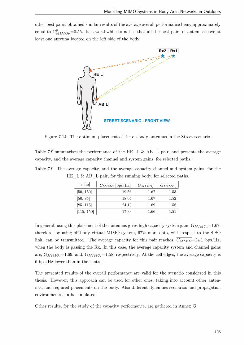
Modelling MIMO Systems in Body Area Networks in Outdoors
other best pairs, obtained similar results of the average overall performance being approximately
equal to CpMIMOP=0.55. It is worthwhile to notice that all the best pairs of antennas have at
least one antenna located on the left side of the body.
Figure 7.14. The optimum placement of the on-body antennas in the Street scenario.
Table 7.9 summarises the performance of the HE_L & AB_L pair, and presents the average
capacity, and the average capacity channel and system gains, for selected paths.
Table 7.9. The average capacity, and the average capacity channel and system gains, for the
HE_L & AB_L pair, for the running body, for selected paths.
x [m] CMIMO [bps/Hz] GMIMOsGMIMOc
[50, 150] 19.56 1.67 1.53
[50, 85] 18.04 1.67 1.52
[85, 115] 24.13 1.69 1.58
[115, 150] 17.33 1.66 1.51
In general, using this placement of the antennas gives high capacity system gain, GMIMOs=1.67,
therefore, by using off-body virtual MIMO system, 67% more data, with respect to the SISO
link, can be transmitted. The average capacity for this pair reaches, CMIMO=24.1 bps/Hz,
when the body is passing the Rx. In this case, the average capacity system and channel gains
are, GMIMOs=1.69, and, GMIMOc=1.58, respectively. At the cell edges, the average capacity is
6 bps/Hz lower than in the centre.
The presented results of the overall performance are valid for the scenario considered in this
thesis. However, this approach can be used for other ones, taking into account other anten-
nas, and required placements on the body. Also different dynamics scenarios and propagation
environments can be simulated.
Other results, for the study of the capacity performance, are gathered in Annex G.
105

x

Chapter 8
Conclusions
This chapter draws final conclusions to the work. The thesis summary, main conclusions, and
recommendations for the future work are presented.
107

8.1 Summary
8.1. Summary
This thesis is organised in eight chapters, which are followed by a set of annexes. Chapter 1,
besides the main objectives and challenges, points out the novelty, and presents the contributions
of this thesis in the development of the models for BANs, and provides as well as the detailed
structure of the thesis.
In Chapter 2, a brief introduction of the wireless communications channel is made, including a
description of main phenomena that take place in the propagation. Also, the review of channel
models is made and the GBSC model is presented in detail, providing the definition of various
radio channel parameters. Finally, the MIMO system is described, and MIMO capacity is
presented and discussed.
In Chapter 3, the state of the art on modelling related to BANs is made. The BAN transmission
channel can be split into three categories including off-body among others (i.e., in-body and
on-body), and as this is the relevant one to this work, its main characteristics are presented.
The electromagnetic properties of the body tissues and variability of the body geometry are
discussed, and possible methods of body modelling are presented (e.g., voxel models) as well.
The concept of wearable antennas and their requirements is introduced, and the importance of
a statistical model for antennas near the body is motivated. At the end of this chapter, the
existing numerical techniques including full wave methods are presented, and the main features
of CST simulation environment, which was used to obtain important results of this thesis, are
described in details.
Chapter 4 proposes a new statistical model to analyse the performance of wearable antennas
in BANs. Firstly, the simple model based on image theory is introduced, and the method to
calculate a statistical radiation pattern of the electric field, depending on the antenna to body
distance distribution, is presented. Then, a patch antenna near the body has been modelled in
CST with various meshing options, in order to select the optimum one in terms of complexity and
accuracy. In this chapter, the study of correlation between signals captured by wearable antennas
is presented as well. Finally, the novel model to account for the realistic body movements is
described.
In Chapter 5, the results obtained from the developed models, accounting for the body coupling
(using theoretical, numerical and practical approaches), signal correlation and body dynamics
are presented and analysed. The results presented in this chapter are also taken as an input for
the developed model of a BAN radio channel.
In Chapter 6, the developed channel model for BANs is presented, and its implementation
in the developed simulator is also described. The whole off-body radio channel is considered
using the GBSC model, and the influence of the propagation environment is taken into account.
Fundamental assessment procedures are described, and a comparison with the measurement
data is provided.
108

Modelling MIMO Systems in Body Area Networks in Outdoors
In Chapter 7, the results from simulations of street scenario are presented, followed by a deep
statistical analysis of obtained radio channel parameters for off-body communication. The per-
formance analysis of MIMO system in various scenarios and configurations is presented as well.
The selection of the best on-body placements of antennas is done, based on the obtained values
for MIMO capacity.
Finally, in the current chapter, thesis summary, main conclusions, and recommendations for
future work are presented.
8.2. Main Results
The link budget for BANs has to be redefined, therefore, new parameters have to be accounted
for, e.g., antenna gain pattern changes, tissue absorption, transmitted power limited by the safe
margins, influence of body dynamics, and the distance between antenna and the body. Moreover,
a cross-layer perspective for BANs is required, which comprises cooperation and knowledge
sharing between the various system layers. This thesis stresses the core position of the Radio
Channel on the overall system, prompting the strong influence of the human body, addressing
the wide range of BANs scenarios and discussing strategies to improve connectivity problems
(e.g., smart deployment of on-body antennas). In general, a good and deep understanding of
the Radio Channel models in BANs can help improving the QoS of applications.
The novel aspect of this thesis is a statistical analysis of the gain patterns of an antenna,
calculated at different distances between antenna and body. This approach allows one to consider
the antenna gain pattern no longer as a deterministic, but rather stochastic, component of the
link budget, when developing Radio Channel models for BANs.
This can be evaluated using a very simple model based on image theory, which gives a glimpse
of the possible range of changes in the radiation pattern of the electric field. A comprehensive
statistical study on the variations of radiation patterns was carried out for various scenarios
(i.e., frequencies, body sizes, and tissues). When the antenna is located over an ellipse, for a
Uniform Distribution of the distance between antenna and body, the average radiation pattern
is slightly changing among scenarios. The change of the average radiation pattern is a little
more visible for the Rayleigh Distribution, especially for 0.915 GHz, where the antenna to body
distance is changing only a little compared to the wavelength. The standard deviation of the
radiation pattern varies significantly over radiation angles, and also for various frequencies and
tissues. This confirms the validity of the proposed concept of an antenna statistical model.
Among analysed tissues, Muscle has the highest influence (i.e., the highest permittivity and
conductivity) whereas Fat has the lowest one. In general, the standard deviation of the average
radiation pattern is higher for the perpendicular polarisation than for the parallel one.
However, it is advised to perform full wave simulations, in order to obtain realistic antenna gain
patterns and account for the body coupling. The influence of the body is the highest when
109

8.2 Main Results
the antenna is attached to the body, due to the strongest coupling between the body and the
antenna, and reduction of the antenna radiation efficiency. As the main relative variations of
the gain pattern are observed in the backward direction, where the radiation level is very low,
the Pattern Weighted Difference (PWD) is always lower than the Pattern Average Difference
(PAD). In the case when the antenna is located near the Chest with a Rayleigh Distribution, the
PWD can reach 11%, and the the PAD can be as high as 24%, relative to the isolated antenna
case. These results show that the patch is well isolated from the body (i.e., similar gain for
different placements and low standard deviation), which will ensure stability of the system.
The measurement campaign complemented the numerical study, providing results from the whole
complex BAN channel, in an anechoic chamber. Results from measurements are in line with the
CST ones, showing that, in the area of interest for off-body communications, no large changes
between the two approaches are observed.
The difference between received signals captured by wearable antennas in a BAN is evaluated
by the cross-correlation coefficient. The statistical study is performed for various separations of
antennas from the body, which determine the coupling between the body and the antenna. In
a multipath environment, multiple copies of the signal can arrive from an arbitrary direction,
however, in this work the components are investigated separately (i.e., one at the time). The
wearable antennas are placed with different distances to the body in the range [0, 2λ] (i.e., 11
samples uniformly distributed), and the wave is coming from a direction in the range [0◦, 180◦]
(i.e., 36 samples uniformly distributed). For a multiple antennas system, the cross-correlation
between signals is an important measure of the spatial diversity, indicating possible gains of the
MIMO system. The average and standard deviation of cross-correlation are analysed for various
pairs of antennas, which can be split into 3 classes: Co-Directed (CD), Cross-Directed (XD) and
Opposite-Directed (OD). As expected, the cross-correlation is the lowest for antennas located
on different sides of the body (i.e., OD) equal to 0.67, and is the highest for the antennas on the
same side (i.e., CD) equal to 0.95. Therefore, in the case of OD class, the diversity gain should
be higher than for the CD one. The largest variations in average cross-correlation are observed
for the XD class, which is also characterised by the highest standard deviation, equal to 0.13.
In this case, depending on the azimuth, the signals received from the on-body antennas can be
either low or highly correlated. A low cross-correlation is obtained when an antenna is in LoS
with the incoming wave, while the other is shadowed by the body (which is determined by the
placement of the antenna and its distance to the body, as well as the direction of the incoming
wave). In general, the direction has a more significant impact on the cross-correlation than the
distance between the antenna and the body.
Additionally, this thesis presents a very realistic model of body dynamics, and the corresponding
influence on antenna gain patterns from a statistical viewpoint. By using this method, it is
possible to describe and include body movement scenarios in Radio Channel simulators. This
is of great importance, as antenna rotation has a huge impact on the performance of the whole
transmission channel. Due to the movement of the antenna located at the BAN side of the radio
110

Modelling MIMO Systems in Body Area Networks in Outdoors
link, the antenna located at the other side of the link captures significant signal variations, and
changes in the angular power profile. The gain patterns are significantly modified by the body
movement, which depend on the antenna placement. As expected, when the antenna is mounted
on the Arm, the standard deviation of the change in normal to the body surface is the highest
among all placements, reaching 19◦ and 37◦ for the running body, for elevation and azimuth
angles, respectively. The standard deviation for the walking body is much smaller compared to
the running one, for all antenna placements, being always less than 4◦. Therefore, the walking
body does not have a significant influence on the gain pattern of the patch. The Kumaraswamy
Distribution has been considered as the best fit for variations in the direction normal to the
surface. In general, when the antenna is placed on a very dynamic body segment (e.g., Arm and
running body), the maximum gain of average gain pattern is reduced. Moreover, the shape of
the gain pattern is more uniform relative to the static body, and the standard deviation is very
high. This mean that body dynamics can have a very important impact on the performance of
the whole off-body link, especially for highly dynamic scenarios (e.g., running body).
The influence of the propagation environment can be taken into account, including previously
obtained antenna gains and body dynamic characteristics, in the GBSC model. Therefore, a
flexible and novel method to model Radio Channels in off-body communications is proposed.
Using this approach, both the temporal (i.e., delay spread) and angular (i.e., angular spread)
parameters can be characterised. Also, the study of the MIMO capacity for various antenna
locations can be performed, and the optimum configurations can be selected. The developed
models and algorithms are not system dependent, so they can be used for other systems, and
not just for the one chosen for example.
A BAN with patch antennas operating at 2.45 GHz and 9 possible locations on the body has
been analysed: TO_F, WA_F, HE_F, HE_B, HE_L, HE_R, AB_L, AB_R and TO_B.
Simulations have been performed for one propagation environment scenario (i.e., street), and
two body movements (i.e., walking and running bodies).
Basic Radio Channel parameters, as the propagation conditions (i.e., LoS, NLoS and Mixed), the
received power, the delay spread and DoA spread are obtained, and a statistical analysis of results
is provided. As expected, output parameters strongly depend on the body movement, especially
when the antenna is located on AB_L. For the running body, the propagation conditions change
rapidly, and 9 dB deep fades in the average received power are captured, in contrast to 4 dB for
the walking body in the cell edge. Therefore, the body movement can determine the connectivity
of the radio link. The lowest average delay spread, 61 ns, is obtained for the AB_L antenna
when the body is closed to the Rx. In this case, the multipath channel richness is low (i.e.,
the dominant role has the LoS component). As expected, when the antenna is in NLoS, the
average standard deviation of the delay spread is the highest, reaching 40 ns in the cell edge
(i.e., strong contribution from the MPCs). The average DoA spread depends on the location of
the body in the cell, being minimum when the body is close to the Rx (i.e., for AB_L it is 20◦,
and [33◦, 39◦] for other placements).
111

8.2 Main Results
In order to measure how much a signal in an on-body antenna behaves like another, the envelope
correlation is calculated. The largest differences between signals are found for antennas located
on the front and back sides (the absolute average envelope correlation is equal to 0.30, which is
below 0.70 that can be used as the guideline for successful diversity operation). Therefore, the
independent fading of the signals (i.e., high diversity gain) can be obtained, by the placement
of the antennas in the opposite sides of the body.
In this thesis, the correlations between CIRs are obtained, and a statistical analysis of results is
provided. As expected, the correlation is the lowest for antennas located on different sides of the
body (i.e., OD), equal to 0.28, and is the highest for antennas on the same side (i.e., CD), equal
to 0.56. The lowest correlation is obtained for HE_B & WA_F, equal to 0.19, and this placement
provides the best diversity among the analysed scenarios. However, because of the strong power
imbalance, this does not lead to a good performance of the MIMO system. In general, when
one antenna is located on the right side of the body (i.e., NLoS conditions), the correlation
is lower, being similar for all classes, [0.34, 0.44]. Due to the randomness of the propagation
environment, large variations of body postures, and changes of body location in the cell, the
standard deviation of the correlation is always above 0.16. The largest standard deviation was
obtained for the XD and OD classes and the running body, equal to 0.23. Therefore, the state
of the channel strongly depends on the body dynamics and general position of the body in
reference to the Rx.
Moreover, the 2×2 MIMO capacity for 36 possible combinations was obtained, and a statistical
analysis of results is provided. The average capacity strongly depends on the power imbalance
between antennas. Because the Rx is located on the left, the average capacity is the highest
when both antennas are located on the left side of the body (i.e., HE_L & AB_L), equal to
19.2 bps/Hz. When one antenna is located on the Arm (i.e., AB_L), the changes of the direction
of maximum radiation of antenna, results in a difference of 6 bps/Hz during a single running
period. Again, this confirms the strong impact of body dynamics on the overall performance.
For antennas located on the right, the average capacity is lower (i.e., close to the bottom bound),
however, the standard deviation is also low. As expected, the lowest standard deviation, equal
to 2.9 bps/Hz, is obtained for the OD antennas. In this case, due to strong power imbalances
between antennas, the system can not benefit from the capacity gains, but can improve the
outage of the Radio Channel exploring diversity gain. In general, for the considered scenario,
the results indicates that the HE_L & AB_L pair outperforms other ones, with average overall
performance being 0.64. The main reason is good propagation conditions along body movement
in the cell (i.e., most of the time antennas are in LoS with the Rx), and low power imbalance.
The final conclusion of this thesis, is that the usage of virtual MIMO in BANs can benefit from
the capacity gain and enhancement of the overall performance of off-body links. Moreover, this
thesis stresses the importance of the statistical modelling of the antennas, which has to be taken
into account, when developing a real system for off-body communications. From the results
presented in this thesis, one can conclude that body dynamics play a dominant role in the BAN
112
Modelling MIMO Systems in Body Area Networks in Outdoors
link budget, especially in the case of highly dynamic scenarios like running body, which can
be even more important in real scenarios of human daily life. In order to minimise the outage
of the system, multiple on-body antennas can be distributed on various locations on the body
(i.e., with different orientation), which increase the independence of links (i.e., decrease the
correlation between them).
8.3. Future Work
One considers that this thesis is an important step towards the development of a general radio
channel model for off-body communications. However, in future work, some improvements can
be done in order to approximate the model to real conditions.
In this study, polarisation is not taken into account, but future studies can build a model for
the polarisation using the same body movement concept. Moreover, it is required to imple-
ment in the simulator the antenna patterns with polarisation, and to analyse body and channel
depolarisation effects.
Another interesting aspect is to develop, and include in modelling of body dynamics, a model
accounting for the shadowing of the body segments (e.g., hands). The model can consider the
attenuation of the body, depending on the type of the tissues and the thickness of the segment.
This approach can also lead to model exposure of the body (i.e., calculation of SAR) coming
from the on-body devices.
Many objects in the environment can change their position in time, which can be emulated by
the appearance, movement, and disappearance of clusters and scatterers. This can be done, by
implementing the velocity vectors for the clusters and scatterers in the simulator.
New types of scenarios can be implemented in the simulator. So far, only ellipsoid and cuboid
scattering regions are included in the simulator. The option to have many overlaying and
different volumes in one environment can be a solution for this problem. Furthermore, the
separated scattering regions, can be associated with different objects having different statistical
properties (i.e., volume distributions and reflection coefficients).
Above all, it is required to perform simulations of a wide range of scenarios, taken from the
measurements sessions, and compare and validate obtained results. This analysis should cover
a wide range of: propagation environments, antenna designs, antenna placements, bodies, and
frequencies. This can be achieved, by establishing cooperation with other researchers working
on BAN channel modelling (i.e., performing measurement of BANs) and participation in various
research projects. The goal of this cooperation should be a common framework between research
institutes, and a common database of results. Finally, the model should be implemented in real
systems and applications.
113

x

Modelling MIMO Systems in Body Area Networks in Outdoors
Annex A. User’s Manual
Before running the simulator application, properly prepared config file containing input para-
meters have to be created. The config file has an XML tree structure, where input parameters
are divided into three main groups (i.e., environment, simulator, system). The structure of the
first section, which defines parameters that describe scenario and control simulator behaviour,
is presented in Figure A.1.
<simulator>
<projectName>street_run</projectName> %name of the project
<scenario>Street</scenario> %scenario name
<scenarioType>Outdoor</scenarioType> %scenario type
<timeFrames>750</timeFrames> %number of the time frames
<runNumber>1</runNumber> %number of simulator runs
<runStart>0</runStart> %starting number
<environmentPeriod>750</environmentPeriod> %environment generation period
<environmentExport>0</environmentExport> %export environment
%0:no, 1:yes
<patternExport>0</patternExport> %export antenna patterns
%0:no, 1:yes
</simulator>
Figure A.1. Parameters describing scenario and controlling simulator’s behaviour.
The structure of the environment section, which describes the shape of the scattering region,
and defines numbers of clusters and scatterers, is presented in Figure A.2.
<environment>
<numberClusters>10</numberClusters> %number of clusters
<numberScatterers>3</numberScatterers> %number of scatterers
<maxBounce>2</maxBounce> %maximum number of bounces
<xLen>200</xLen> %x dimension [m]
<yLen>20</yLen> %y dimension [m]
<zLen>10</zLen> %z dimension [m]
<rClst>1</rClst> %cluster radius [m]
<shapeType>2</shapeType> %scattering region shape
%0:cuboid, 1:sphere, 2:ellipsoid
<aElipse>100</aElipse> %dimension x axis [m]
<bElipse>10</bElipse> %dimension y axis [m]
<cElipse>9</cElipse> %dimension z axis [m]
<xElipse>100</xElipse> %x: ellipse centre [m]
<yElipse>10</yElipse> %y: ellipse centre [m]
<zElipse>0</zElipse> %z: ellipse centre [m]
</environment>
Figure A.2. Parameters describing propagation environment.
The last group defines system parameters like carrier frequency and transmitted power, Fi-
gure A.3. Moreover, parameters within this groups define the MIMO system (i.e., numbers
of input and output antennas, and spacing between antennas). The radiation patterns can be
loaded from XML files, and allocated to antennas. For the body side, the movement scenario
115

User’s Manual
can be loaded from XML files, which contain the position of the antennas during the movement
(i.e., in frame-by-frame manner).
<system>
<frequency>2400000000</frequency> %carrier frequency [Hz]
<txPower>1</txPower> %Tx power [W]
<txNumber>2</txNumber> %number of Tx antennas
<rxNumber>2</rxNumber> %number of Rx antennas
<xTx>50</xTx><yTx>10</yTx><zTx>0</zTx> %(x, y, z) center position of Tx
<dxTx>0</dxTx><dyTx>0</dyTx><dzTx>0</dzTx> %automatic location of Tx antennas
%(only when modeTx=0)
<xRx>100</xRx><yRx>20</yRx><zRx>3</zRx> %(x, y, z) center position of Rx
<dxRx>1</dxRx><dyRx>0</dyRx><dzRx>0</dzRx> %automatic location of Rx antennas
%(only when modeRx=0)
<patterns>2</patterns> %number of gain patterns to load
<pattern1>antenna_iso.xml</pattern1> %1st file with gain pattern
<pattern2>antenna_head.xml</pattern2> %2nd file with gain pattern
<motionTx>motion_run_25.xml</motionTx> %movement file for Tx
<modeTx>2</modeTx> %movement mode of Tx
%0:taken by dxTx, dyTx dzTx
%1:manual
%2:taken from motionTx file
<Tx1> %parameters for 1st Tx antenna
<patId>1</patId> %selection of the gain pattern
<location>TO_F</location> %antenna on-body placement
</Tx1>
<Tx2> %parameters for 2nd Tx antenna
<patId>1</patId> %selection of the gain pattern
<location>HE_F</location> %antenna on-body placement
</Tx2>
<modeRx>0</modeRx> %movement mode of Rx
%0:taken by dxRx, dyRx dzRx
%1:manual
%2:taken from motionRx file
<Rx1> %parameters for 1st Rx antenna
<patId>0</patId> %selection of the gain pattern
<rotTheta>0</rotTheta> %rotation in elevation plane
<rotPhi>0</rotPhi> %rotation in azimuth plane
</Rx1>
<Rx2> %parameters for 2nd Rx antenna
<patId>0</patId> %selection of the gain pattern
<rotTheta>0</rotTheta> %rotation in elevation plane
<rotPhi>0</rotPhi> %rotation in azimuth plane
</Rx2>
</system>
Figure A.3. Parameters describing system parameters including configuration and properties of
MIMO antennas, and body movement scenario.
116

Modelling MIMO Systems in Body Area Networks in Outdoors
The antenna parameters are defined using the XML file, where the gain pattern is defined in all
directions, and some general information are provided, Figure A.4.
<antenna>
<patternType>head_location</patternType> %type of the pattern
<pattern> %THETA in [0 180]
%PHI in [0 360]
<t0>
<p0>0.286061377957</p0> %gain for THETA=0 and PHI=0
(...) %definition for other PHI
<p360>0.286061377957</p360>
</t0>
(...) %definition for other THETA
<t180>
<p0>0.155544450691</p0>
(...)
<p360>0.155544450691</p360>
</t180>
</pattern>
<patternParams>
<gmin>-30.9220211085</gmin> %minimum of antenna gain
<gminTheta>105</gminTheta> %THETA direction of minimum gain
<gminPhi>330</gminPhi> %PHI direction of minimum gain
<gmax>6.2938306166</gmax> %maximum of antenna gain
<gmaxTheta>90</gmaxTheta> %THETA direction of maximum gain
<gmaxPhi>180</gmaxPhi> %PHI direction of maximum gain
</patternParams>
</antenna>
Figure A.4. Definition of the antenna gain pattern.
117

User’s Manual
The body movement including detailed information about the antennas locations and orienta-
tions (i.e., antennaXX ), body skeleton nodes positions (i.e., nodeXX ), and body position and
orientation (i.e., body) is defined using the XML file, Figure A.5.
<motion>
<motionName>run</motionName> %name of the body motion
<antenna1> %antenna location on the body
<antennaName>AB_L</antennaName> %antenna placement
<frame0> %first time frame
<t>29.0398230679</t> %antenna elevation rotation [deg]
<p>58.4842542678</p> %antenna azimuth rotation [deg]
<x>34.939964538</x> %x position [cm]
<y>18.0048595714</y> %y position [cm]
<z>106.422218218</z> %z position [cm]
</frame0>
(...) %definition for other time frames
</antenna1>
(...) %definition for other antennas
<node0> %node location in reference to body
<nodeName>hip</nodeName> %body node name
<frame0> %first time frame
<x>-0.13740384</x> %x position [cm]
<y>-5.12231386</y> %y position [cm]
<z>102.01250362</z> %z position [cm]
</frame0>
(...) %definition for other time frames
</node0>
<body> %body position in the cell
<frame0> %first time frame
<t>0</t> %body elevation rotation [deg]
<p>-90</p> %body azimuth rotation [deg]
<x>0</x> %x position [cm]
<y>0</y> %y position [cm]
<z>0</z> %z position [cm]
</frame0>
(...) %definition for other time frames
</body>
<motionFrames>30</motionFrames> %number of time frames
<motionAntennas>5</motionAntennas> %number of antennas
<skeletonNodes>27</skeletonNodes> %number of body nodes
</motion>
Figure A.5. Definition of the body movement scenario.
118

Modelling MIMO Systems in Body Area Networks in Outdoors
Annex B. Tissues Properties
Electric properties of selected body tissues for 0.915, 2.45 and 5.8 GHz are presented in Table B.1.
Table B.1. Electric properties of selected body tissues.0.915 GHz 2.45 GHz 5.8 GHz
εrb σb [S/m] δp [cm] εrb σb [S/m] δp [cm] εrb σb [S/m] δp [cm]
Aorta 44.740 0.701 5.125 42.530 1.435 2.430 38.230 4.345 0.767
Bladder 18.920 0.385 6.112 18.000 0.685 3.318 16.240 1.857 1.169
Blood 61.310 1.545 2.768 58.260 2.545 1.612 52.540 6.506 0.602
BodyFluid 68.900 1.641 2.755 68.210 2.478 1.785 64.780 6.674 0.648
BoneCancellous 20.760 0.344 7.131 18.550 0.805 2.874 15.390 2.148 0.991
BoneCortical 12.440 0.145 12.980 11.380 0.394 4.578 9.674 1.154 1.454
BoneMarrow 5.501 0.041 30.760 5.297 0.095 12.880 4.963 0.285 4.167
BrainGreyMatter 52.650 0.949 4.122 48.910 1.808 2.072 44.000 4.987 0.717
BrainWhiteMatter 38.840 0.595 5.618 36.170 1.215 2.647 32.620 3.494 0.880
Cartilage 42.600 0.789 4.460 38.770 1.756 1.908 32.150 4.891 0.631
Cerebellum 49.350 1.270 3.025 44.800 2.101 1.715 39.980 4.995 0.684
CerebroSpinalFluid 68.610 2.419 1.914 66.240 3.458 1.272 60.470 7.840 0.537
Cervix 49.750 0.964 3.952 47.610 1.726 2.141 43.360 4.803 0.738
Colon 57.870 1.087 3.776 53.880 2.038 1.930 48.460 5.570 0.674
Cornea 55.170 1.401 2.896 51.620 2.295 1.683 46.530 5.664 0.650
Duodenum 65.020 1.193 3.643 62.160 2.211 1.909 56.480 6.314 0.641
Dura 44.390 0.966 3.741 42.030 1.669 2.084 37.880 4.309 0.770
EyeSclera 55.230 1.173 3.434 52.630 2.033 1.913 47.810 5.466 0.682
Fat 5.460 0.051 24.230 5.280 0.105 11.700 4.955 0.293 4.048
Gland 59.650 1.044 3.982 57.200 1.968 2.056 52.050 5.721 0.679
Heart 59.800 1.238 3.382 54.810 2.256 1.761 48.950 5.862 0.644
Kidney 58.560 1.401 2.975 52.740 2.429 1.609 46.750 5.896 0.627
Lens 46.550 0.798 4.601 44.630 1.504 2.376 40.690 4.370 0.785
Liver 46.760 0.861 4.282 43.030 1.686 2.086 38.130 4.642 0.718
LungDeflated 51.370 0.864 4.463 48.380 1.683 2.212 43.750 4.821 0.739
LungInflated 21.970 0.459 5.527 20.480 0.804 3.018 18.510 2.077 1.116
Lymph 59.650 1.044 3.982 57.200 1.968 2.056 52.050 5.721 0.679
Muscle 55.000 0.948 4.210 52.730 1.739 2.233 48.480 4.962 0.754
Nail 12.440 0.145 12.980 11.380 0.394 4.578 9.674 1.154 1.454
Nerve 32.490 0.578 5.316 30.140 1.089 2.701 27.220 2.941 0.954
Ovary 50.360 1.298 2.988 44.700 2.264 1.594 38.690 5.284 0.638
Pancreas 59.650 1.044 3.982 57.200 1.968 2.056 52.050 5.721 0.679
Prostate 60.510 1.216 3.459 57.550 2.168 1.875 52.210 5.948 0.655
Retina 55.230 1.173 3.434 52.630 2.033 1.913 47.810 5.466 0.682
SkinDry 41.330 0.872 3.995 38.010 1.464 2.257 35.110 3.717 0.857
SkinWet 46.020 0.850 4.303 42.850 1.592 2.203 38.620 4.342 0.771
SpinalChord 32.490 0.578 5.316 30.140 1.089 2.701 27.220 2.941 0.954
Spleen 57.090 1.280 3.205 52.450 2.238 1.738 46.940 5.672 0.652
Stomach 65.020 1.193 3.643 62.160 2.211 1.909 56.480 6.314 0.641
Tendon 45.800 0.724 5.017 43.120 1.685 2.090 36.750 5.255 0.627
Thymus 59.650 1.044 3.982 57.200 1.968 2.056 52.050 5.721 0.679
Thyroid 59.650 1.044 3.982 57.200 1.968 2.056 52.050 5.721 0.679
Tongue 55.230 0.942 4.245 52.630 1.803 2.153 47.810 5.235 0.711
Tooth 12.440 0.145 12.980 11.380 0.394 4.578 9.674 1.154 1.454
Trachea 41.970 0.776 4.504 39.730 1.449 2.330 35.940 4.080 0.792
Uterus 61.060 1.276 3.315 57.810 2.247 1.815 52.350 6.047 0.645
119

CST Simulations
Annex C. CST Simulations
This annex includes the gain patterns of a patch antenna [MeCa06] operating in the 2.45 GHz
band, which was simulated in CST, with different distances to the voxel body model. Simulations
were performed for 4 antenna placements, i.e., Head, Chest, Arm and Leg, and the distance
from the body surface in range [0, 2λ], Figure C.1.
−20 dBi −10 dBi 0 dBi +10 dBi −30 dBi
−150o
30o
−120o
60o
−90o
90o
−60o
120o
−30o
150o
0o
180o
Isolated Antenna
h=0λ
h=1/2λ
h=λ
h=3/2λ
h=2λ
−20 dBi −10 dBi 0 dBi +10 dBi −30 dBi
−150o
30o
−120o
60o
−90o
90o
−60o
120o
−30o
150o
0o
180o
Isolated Antenna
h=0λ
h=1/2λ
h=λ
h=3/2λ
h=2λ
(a) Head (b) Chest
−20 dBi −10 dBi 0 dBi +10 dBi −30 dBi
−150o
30o
−120o
60o
−90o
90o
−60o
120o
−30o
150o
0o
180o
Isolated Antenna
h=0λ
h=1/2λ
h=λ
h=3/2λ
h=2λ
−20 dBi −10 dBi 0 dBi +10 dBi −30 dBi
−150o
30o
−120o
60o
−90o
90o
−60o
120o
−30o
150o
0o
180o
Isolated Antenna
h=0λ
h=1/2λ
h=λ
h=3/2λ
h=2λ
(c) Arm (d) Leg
Figure C.1. The gain patterns of a patch antenna near the body with distance in [0, 2λ].
120

Modelling MIMO Systems in Body Area Networks in Outdoors
The statistics of the gain patterns of a patch antenna, for the Uniform distance Distribution, in
[0, 2λ]), are presented in Figure C.2.
−20 dBi −10 dBi 0 dBi +10 dBi −30 dBi
−150o
30o
−120o
60o
−90o
90o
−60o
120o
−30o
150o
0o
180o
Isolated
Average
Average + STD
Min
Max
−20 dBi −10 dBi 0 dBi +10 dBi −30 dBi
−150o
30o
−120o
60o
−90o
90o
−60o
120o
−30o
150o
0o
180o
Isolated
Average
Average + STD
Min
Max
(a) Head (b) Chest
−20 dBi −10 dBi 0 dBi +10 dBi −30 dBi
−150o
30o
−120o
60o
−90o
90o
−60o
120o
−30o
150o
0o
180o
Isolated
Average
Average + STD
Min
Max
−20 dBi −10 dBi 0 dBi +10 dBi −30 dBi
−150o
30o
−120o
60o
−90o
90o
−60o
120o
−30o
150o
0o
180o
Isolated
Average
Average + STD
Min
Max
(c) Arm (d) Leg
Figure C.2. The statistics of the gain patterns of a patch antenna, for the Uniform distance
Distribution.
121

CST Simulations
The statistics of the gain patterns of a patch antenna, for the Rayleigh distance Distribution,
with a mode of 2 cm, are presented in Figure C.3.
−20 dBi −10 dBi 0 dBi +10 dBi −30 dBi
−150o
30o
−120o
60o
−90o
90o
−60o
120o
−30o
150o
0o
180o
Isolated
Average
Average + STD
Min
Max
−20 dBi −10 dBi 0 dBi +10 dBi −30 dBi
−150o
30o
−120o
60o
−90o
90o
−60o
120o
−30o
150o
0o
180o
Isolated
Average
Average + STD
Min
Max
(a) Head (b) Chest
−20 dBi −10 dBi 0 dBi +10 dBi −30 dBi
−150o
30o
−120o
60o
−90o
90o
−60o
120o
−30o
150o
0o
180o
Isolated
Average
Average + STD
Min
Max
−20 dBi −10 dBi 0 dBi +10 dBi −30 dBi
−150o
30o
−120o
60o
−90o
90o
−60o
120o
−30o
150o
0o
180o
Isolated
Average
Average + STD
Min
Max
(c) Arm (d) Leg
Figure C.3. The statistics of the gain patterns of a patch antenna, for the Rayleigh distance
Distribution.
122
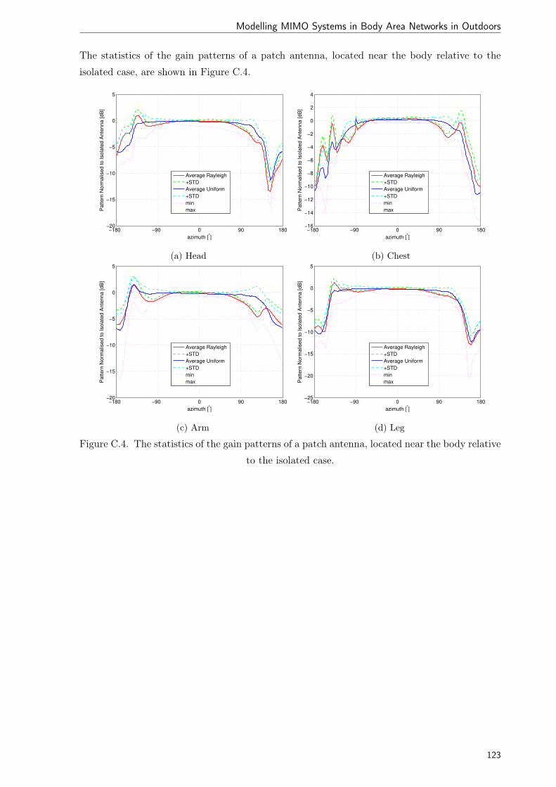
Modelling MIMO Systems in Body Area Networks in Outdoors
The statistics of the gain patterns of a patch antenna, located near the body relative to the
isolated case, are shown in Figure C.4.
−180 −90 0 90 180−20
−15
−10
−5
0
5
azimuth [°]
Pattern
Norm
alis
ed to Isola
ted A
nte
nna [dB
]
Average Rayleigh
+STD
Average Uniform
+STD
min
max
−180 −90 0 90 180−16
−14
−12
−10
−8
−6
−4
−2
0
2
4
azimuth [°]
Pattern
Norm
alis
ed to Isola
ted A
nte
nna [dB
]
Average Rayleigh
+STD
Average Uniform
+STD
min
max
(a) Head (b) Chest
−180 −90 0 90 180−20
−15
−10
−5
0
5
azimuth [°]
Pattern
Norm
alis
ed to Isola
ted A
nte
nna [dB
]
Average Rayleigh
+STD
Average Uniform
+STD
min
max
−180 −90 0 90 180−25
−20
−15
−10
−5
0
5
azimuth [°]
Pattern
Norm
alis
ed to Isola
ted A
nte
nna [dB
]
Average Rayleigh
+STD
Average Uniform
+STD
min
max
(c) Arm (d) Leg
Figure C.4. The statistics of the gain patterns of a patch antenna, located near the body relative
to the isolated case.
123

Body Dynamics
Annex D. Body Dynamics
This annex includes the gain patterns of a patch antenna, [MCCF07], operating at 2.45 GHz,
which is located on the walking or running body.
The statistics of the gain patterns (presented in the body coordinates), for the walking body,
and for the Head, Chest, Arm and Leg placements, are presented in Figure D.1.
−20 dBi −10 dBi 0 dBi +10 dBi −30 dBi
−150o
30o
−120o
60o
−90o
90o
−60o
120o
−30o
150o
0o
180o
Average
Average + STD
Min
Max
−20 dBi −10 dBi 0 dBi +10 dBi −30 dBi
−150o
30o
−120o
60o
−90o
90o
−60o
120o
−30o
150o
0o
180o
Average
Average + STD
Min
Max
(a) Head (b) Chest
−20 dBi −10 dBi 0 dBi +10 dBi −30 dBi
−150o
30o
−120o
60o
−90o
90o
−60o
120o
−30o
150o
0o
180o
Average
Average + STD
Min
Max
−20 dBi −10 dBi 0 dBi +10 dBi −30 dBi
−150o
30o
−120o
60o
−90o
90o
−60o
120o
−30o
150o
0o
180o
Average
Average + STD
Min
Max
(c) Arm (d) Leg
Figure D.1. The statistics of the gain patterns, for the walking body.
124

Modelling MIMO Systems in Body Area Networks in Outdoors
The statistics of the gain patterns (presented in the body coordinates), for the running body,
and for the Head, Chest, Arm and Leg placements, are presented in Figure D.2.
−20 dBi −10 dBi 0 dBi +10 dBi −30 dBi
−150o
30o
−120o
60o
−90o
90o
−60o
120o
−30o
150o
0o
180o
Average
Average + STD
Min
Max
−20 dBi −10 dBi 0 dBi +10 dBi −30 dBi
−150o
30o
−120o
60o
−90o
90o
−60o
120o
−30o
150o
0o
180o
Average
Average + STD
Min
Max
(a) Head (b) Chest
−20 dBi −10 dBi 0 dBi +10 dBi −30 dBi
−150o
30o
−120o
60o
−90o
90o
−60o
120o
−30o
150o
0o
180o
Average
Average + STD
Min
Max
−20 dBi −10 dBi 0 dBi +10 dBi −30 dBi
−150o
30o
−120o
60o
−90o
90o
−60o
120o
−30o
150o
0o
180o
Average
Average + STD
Min
Max
(c) Arm (d) Leg
Figure D.2. The statistics of the gain patterns, for the running body.
125
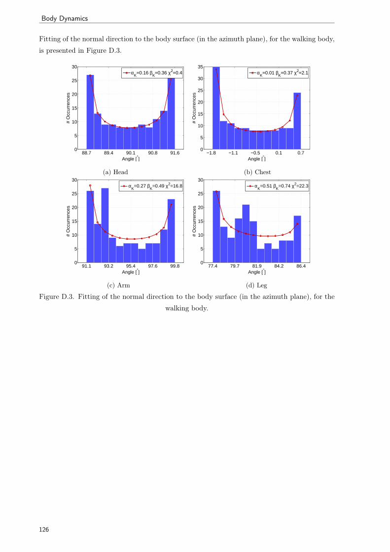
Body Dynamics
Fitting of the normal direction to the body surface (in the azimuth plane), for the walking body,
is presented in Figure D.3.
88.7 89.4 90.1 90.8 91.60
5
10
15
20
25
30
Angle [°]
# O
ccur
renc
es
αK=0.16 β
K=0.36 χ2=0.4
−1.8 −1.1 −0.5 0.1 0.70
5
10
15
20
25
30
35
Angle [°]
# O
ccur
renc
es
αK=0.01 β
K=0.37 χ2=2.1
(a) Head (b) Chest
91.1 93.2 95.4 97.6 99.80
5
10
15
20
25
30
Angle [°]
# O
ccur
renc
es
αK=0.27 β
K=0.49 χ2=16.8
77.4 79.7 81.9 84.2 86.40
5
10
15
20
25
30
Angle [°]
# O
ccur
renc
es
αK=0.51 β
K=0.74 χ2=22.3
(c) Arm (d) Leg
Figure D.3. Fitting of the normal direction to the body surface (in the azimuth plane), for the
walking body.
126

Modelling MIMO Systems in Body Area Networks in Outdoors
Fitting of the normal direction to the body surface (in the elevation plane), for the walking
body, is presented in Figure D.4.
−1.1 −0.6 −0 0.5 1.10
5
10
15
20
25
30
35
Angle [°]
# O
ccur
renc
es
αK=0.14 β
K=0.24 χ2=0.9
−2.9 −2.3 −1.7 −1.2 −0.60
5
10
15
20
25
30
Angle [°]
# O
ccur
renc
es
αK=0.53 β
K=0.81 χ2=13.3
(a) Head (b) Chest
26.1 28.7 31.3 33.9 36.60
5
10
15
20
25
30
35
Angle [°]
# O
ccur
renc
es
αK=0.18 β
K=0.3 χ2=2.4
−6 −3.3 −0.6 2 4.70
5
10
15
20
25
30
35
Angle [°]
# O
ccur
renc
es
αK=0.02 β
K=0.26 χ2=29.4
(c) Arm (d) Leg
Figure D.4. Fitting of the normal direction to the body surface (in the elevation plane), for the
walking body.
127
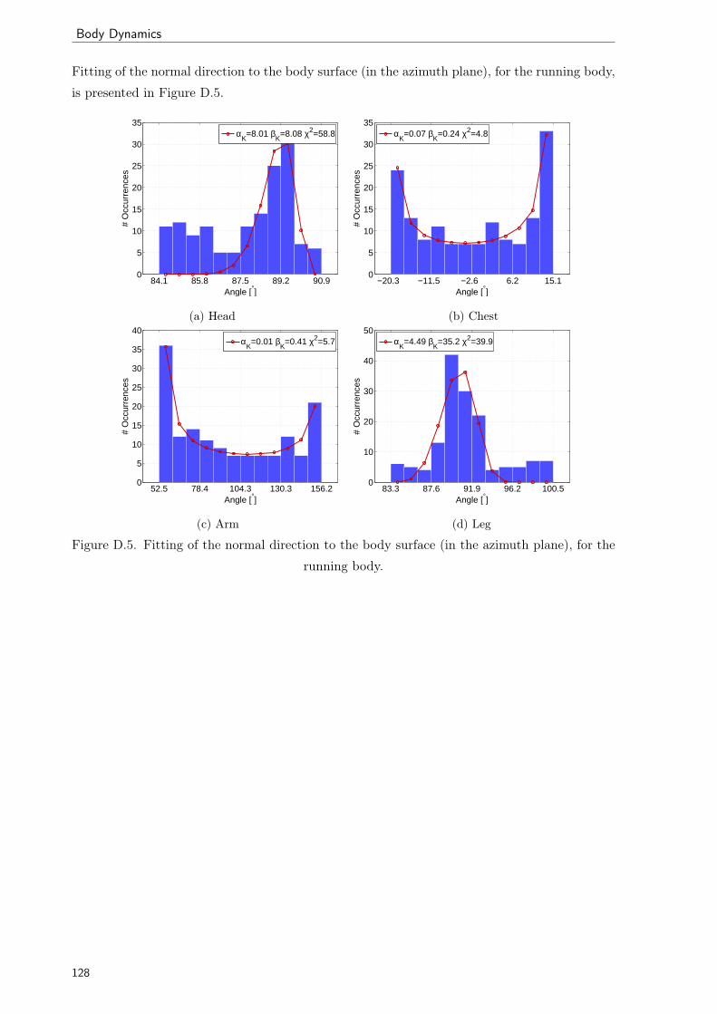
Body Dynamics
Fitting of the normal direction to the body surface (in the azimuth plane), for the running body,
is presented in Figure D.5.
84.1 85.8 87.5 89.2 90.90
5
10
15
20
25
30
35
Angle [°]
# O
ccur
renc
es
αK=8.01 β
K=8.08 χ2=58.8
−20.3 −11.5 −2.6 6.2 15.10
5
10
15
20
25
30
35
Angle [°]
# O
ccur
renc
es
αK=0.07 β
K=0.24 χ2=4.8
(a) Head (b) Chest
52.5 78.4 104.3 130.3 156.20
5
10
15
20
25
30
35
40
Angle [°]
# O
ccur
renc
es
αK=0.01 β
K=0.41 χ2=5.7
83.3 87.6 91.9 96.2 100.50
10
20
30
40
50
Angle [°]
# O
ccur
renc
es
αK=4.49 β
K=35.2 χ2=39.9
(c) Arm (d) Leg
Figure D.5. Fitting of the normal direction to the body surface (in the azimuth plane), for the
running body.
128

Modelling MIMO Systems in Body Area Networks in Outdoors
Fitting of the normal direction to the body surface (in the elevation plane), for the running
body, is presented in Figure D.6.
−1.8 0.3 2.3 4.4 6.40
5
10
15
20
25
30
Angle [°]
# O
ccur
renc
es
αK=1.68 β
K=3.44 χ2=32.7
−15.8 −14.2 −12.6 −11 −9.40
5
10
15
20
25
30
Angle [°]
# O
ccur
renc
es
αK=0.54 β
K=0.86 χ2=89.3
(a) Head (b) Chest
5.4 19 32.6 46.2 59.80
10
20
30
40
50
Angle [°]
# O
ccur
renc
es
αK=0.01 β
K=0.45 χ2=6.8
−4.4 −1 2.5 6 9.40
5
10
15
20
25
30
35
Angle [°]
# O
ccur
renc
es
αK=0.67 β
K=0.81 χ2=56.6
(c) Arm (d) Leg
Figure D.6. Fitting of the normal direction to the body surface (in the elevation plane), for the
running body.
129

Body Dynamics
The average and standard deviation of the gain pattern, in both planes (in the antenna coordi-
nates, where ϕ=0 and ψ=0 corresponds to the direction of maximum radiation), for the walking
and running scenarios, are compared with the static one in Figure D.7, Figure D.8, Figure D.9
and Figure D.10.
(a) static body
(b) average for the walking body (c) standard deviation for the walking body
(d) average for the running body (e) standard deviation for the running body
Figure D.7. The average and standard deviation of the gain pattern for the Arm placement.
(a) static body
(b) average for the walking body (c) standard deviation for the walking body
(d) average for the running body (e) standard deviation for the running body
Figure D.8. The average and standard deviation of the gain pattern for the Chest placement.
130

Modelling MIMO Systems in Body Area Networks in Outdoors
(a) static body
(b) average for the walking body (c) standard deviation for the walking body
(d) average for the running body (e) standard deviation for the running body
Figure D.9. The average and standard deviation of the gain pattern for the Head placement.
(a) static body
(b) average for the walking body (c) standard deviation for the walking body
(d) average for the running body (e) standard deviation for the running body
Figure D.10. The average and standard deviation of the gain pattern for the Leg placement.
131

Radio Channel Parameters
Annex E. Radio Channel Parameters
The average and the standard deviation of the received power for the running body, are presented
in Figure E.1.
50 70 90 110 130 150−80
−75
−70
−65
−60
−55
−50
x [m]
Rx
pow
er[d
Bm
]
HE_F
AB_L
AB_R
TO_B
50 70 90 110 130 1500
1
2
3
4
5
6
7
x [m]
Rx
pow
er[d
Bm
]
HE_F
AB_L
AB_R
TO_B
(a) average (b) standard deviation
Figure E.1. Received power for the running body.
The statistics of the received power for the running body, calculated for selected paths, are
presented in Table E.1.
Table E.1. Received power for the running body, calculated for selected paths.
x [m] propagation PR σPRσPR
[dBm] [dB]
HE_F [50, 150] Mix -64.4 4.8 3.3[50, 85] LoS -60.7 1.1 1.6[85, 115] NLoS -62.1 3.2 2.5[115, 150] NLoS -70.1 2.2 4.7
AB_L [50, 150] Mix -64.8 5.2 2.4[50, 85] Mix -67.4 3.7 2.7[85, 115] Mix -59.1 3.5 1.5[115, 150] Mix -67.0 3.7 2.6
AB_R [50, 150] NLoS -68.3 2.9 3.3[50, 85] NLoS -69.3 2.2 3.2[85, 115] NLoS -66.1 1.7 3.6[115, 150] NLoS -69.2 3.2 3.0
TO_B [50, 150] Mix -64.2 4.8 3.2[50, 85] NLoS -69.8 2.0 4.5[85, 115] Mix -61.7 3.4 2.7[115, 150] LoS -60.8 1.2 1.7
132

Modelling MIMO Systems in Body Area Networks in Outdoors
The average and the standard deviation of the received power for the walking body, are presented
in Figure E.2.
50 70 90 110 130 150−80
−75
−70
−65
−60
−55
−50
x [m]
Rx
pow
er[d
Bm
]
HE_F
AB_L
AB_R
TO_B
50 70 90 110 130 1500
1
2
3
4
5
6
x [m]
Rx
pow
er[d
Bm
]
HE_F
AB_L
AB_R
TO_B
(a) average (b) standard deviation
Figure E.2. Received power for the walking body.
The statistics of the received power for the walking body, calculated for selected paths, are
presented in Table E.2.
Table E.2. Received power for the walking body, calculated for selected paths.
x [m] propagation PR σPRσPR
[dBm] [dB]
HE_F [50, 150] Mix -65.0 5.7 3.4[50, 85] LoS -60.6 1.1 1.4[85, 115] NLoS -62.2 3.4 2.7[115, 150] NLoS -72.0 2.6 4.9
AB_L [50, 150] Mix -64.7 5.5 2.1[50, 85] NLoS -68.3 2.9 2.5[85, 115] Mix -57.8 2.9 1.2[115, 150] NLoS -67.1 3.0 2.2
AB_R [50, 150] NLoS -69.4 2.0 3.1[50, 85] NLoS -70.1 1.6 3.0[85, 115] NLoS -67.5 0.7 3.5[115, 150] NLoS -70.4 1.9 3.0
TO_B [50, 150] Mix -64.3 5.0 3.2[50, 85] NLoS -70.5 2.1 4.5[85, 115] Mix -61.6 3.1 2.6[115, 150] LoS -60.6 1.1 1.5
133
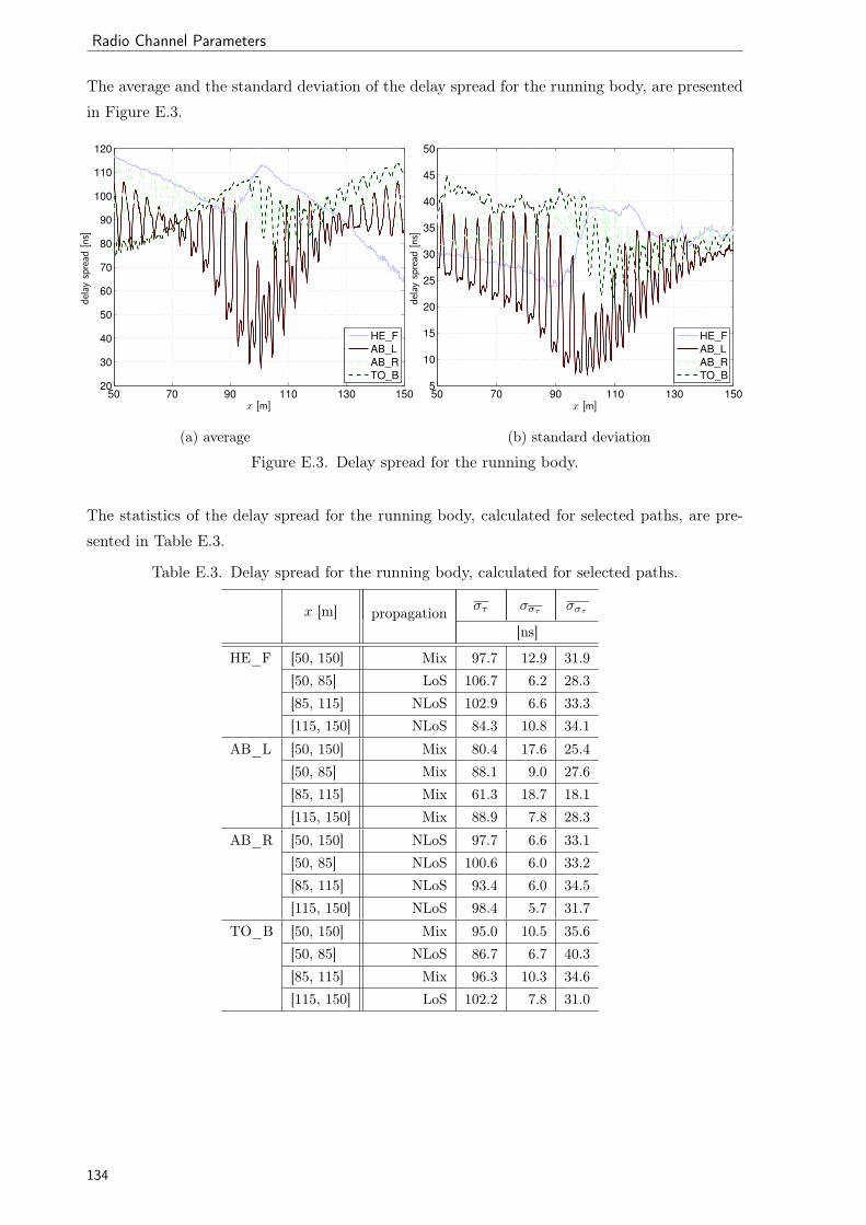
Radio Channel Parameters
The average and the standard deviation of the delay spread for the running body, are presented
in Figure E.3.
50 70 90 110 130 15020
30
40
50
60
70
80
90
100
110
120
x [m]
delay
spre
ad[n
s]
HE_F
AB_L
AB_R
TO_B
50 70 90 110 130 1505
10
15
20
25
30
35
40
45
50
x [m]delay
spre
ad[n
s]
HE_F
AB_L
AB_R
TO_B
(a) average (b) standard deviation
Figure E.3. Delay spread for the running body.
The statistics of the delay spread for the running body, calculated for selected paths, are pre-
sented in Table E.3.
Table E.3. Delay spread for the running body, calculated for selected paths.
x [m] propagation στ σστ σστ
[ns]
HE_F [50, 150] Mix 97.7 12.9 31.9[50, 85] LoS 106.7 6.2 28.3[85, 115] NLoS 102.9 6.6 33.3[115, 150] NLoS 84.3 10.8 34.1
AB_L [50, 150] Mix 80.4 17.6 25.4[50, 85] Mix 88.1 9.0 27.6[85, 115] Mix 61.3 18.7 18.1[115, 150] Mix 88.9 7.8 28.3
AB_R [50, 150] NLoS 97.7 6.6 33.1[50, 85] NLoS 100.6 6.0 33.2[85, 115] NLoS 93.4 6.0 34.5[115, 150] NLoS 98.4 5.7 31.7
TO_B [50, 150] Mix 95.0 10.5 35.6[50, 85] NLoS 86.7 6.7 40.3[85, 115] Mix 96.3 10.3 34.6[115, 150] LoS 102.2 7.8 31.0
134

Modelling MIMO Systems in Body Area Networks in Outdoors
The average and the standard deviation of the delay spread for the walking body, are presented
in Figure E.4.
50 70 90 110 130 15020
30
40
50
60
70
80
90
100
110
120
x [m]
delay
spre
ad[n
s]
HE_F
AB_L
AB_R
TO_B
50 70 90 110 130 1505
10
15
20
25
30
35
40
45
50
55
x [m]
delay
spre
ad[n
s]
HE_F
AB_L
AB_R
TO_B
(a) average (b) standard deviation
Figure E.4. Delay spread for the walking body.
The statistics of the delay spread for the walking body, calculated for selected paths, are pre-
sented in Table E.4.
Table E.4. Delay spread for the walking body, calculated for selected paths.
x [m] propagation στ σστ σστ
[ns]
HE_F [50, 150] Mix 95.0 8.4 34.1[50, 85] LoS 95.6 6.1 24.3[85, 115] NLoS 96.8 10.7 37.8[115, 150] NLoS 92.7 7.6 38.9
AB_L [50, 150] Mix 69.7 21.0 19.1[50, 85] NLoS 80.5 9.1 21.2[85, 115] Mix 42.0 11.0 10.3[115, 150] NLoS 82.6 11.2 22.3
AB_R [50, 150] NLoS 92.3 6.4 26.2[50, 85] NLoS 91.1 3.2 27.9[85, 115] NLoS 85.9 2.9 26.2[115, 150] NLoS 98.8 4.6 24.5
TO_B [50, 150] Mix 96.6 9.8 33.3[50, 85] NLoS 93.6 11.4 43.4[85, 115] Mix 96.6 9.5 30.0[115, 150] LoS 99.6 6.8 22.7
135

Radio Channel Parameters
The average and the standard deviation of the DoA spread for the running body, are presented
in Figure E.5.
50 70 90 110 130 15010
15
20
25
30
35
40
45
50
x [m]
angularsp
read
[◦]
HE_F
AB_L
AB_R
TO_B
50 70 90 110 130 1504
6
8
10
12
14
16
18
20
x [m]an
gularsp
read
[◦]
HE_F
AB_L
AB_R
TO_B
(a) average (b) standard deviation
Figure E.5. DoA spread for the running body.
The statistics of the DoA spread for the Run scenario, calculated for selected paths, are presented
in Table E.5.
Table E.5. DoA spread for the running body, calculated for selected paths.
x [m] propagation σDoA σσDoAσσDoA
[◦]
HE_F [50, 150] Mix 39.5 4.4 13.0[50, 85] LoS 44.0 2.9 10.9[85, 115] NLoS 35.8 3.1 11.2[115, 150] NLoS 38.2 2.2 16.0
AB_L [50, 150] Mix 35.4 9.6 10.9[50, 85] Mix 40.7 4.6 12.9[85, 115] Mix 22.8 6.2 7.6[115, 150] Mix 40.9 3.8 11.2
AB_R [50, 150] NLoS 41.2 4.3 12.6[50, 85] NLoS 43.8 2.3 13.4[85, 115] NLoS 35.9 2.5 12.4[115, 150] NLoS 43.1 2.7 12.0
TO_B [50, 150] Mix 39.0 4.5 12.7[50, 85] NLoS 38.4 0.5 16.3[85, 115] Mix 34.7 3.7 11.6[115, 150] LoS 43.4 3.1 9.0
136

Modelling MIMO Systems in Body Area Networks in Outdoors
The average and the standard deviation of the DoA spread for the walking body are presented
in Figure E.6.
50 70 90 110 130 15010
15
20
25
30
35
40
45
50
55
x [m]
angularsp
read
[◦]
HE_F
AB_L
AB_R
TO_B
50 70 90 110 130 1506
8
10
12
14
16
18
20
x [m]
angularsp
read
[◦]
HE_F
AB_L
AB_R
TO_B
(a) average (b) standard deviation
Figure E.6. DoA spread for the walking body.
The statistics of the DoA spread for the walking body, calculated for selected paths, are presented
in Table E.6.
Table E.6. DoA spread for the walking body, calculated for selected paths.
x [m] propagation σDoA σσDoAσσDoA
[◦]
HE_F [50, 150] Mix 39.4 4.1 13.4[50, 85] LoS 44.1 2.5 11.3[85, 115] NLoS 35.2 2.1 11.4[115, 150] NLoS 38.2 0.9 16.5
AB_L [50, 150] Mix 34.1 10.3 11.1[50, 85] NLoS 39.6 4.9 12.7[85, 115] Mix 20.2 4.7 9.0[115, 150] NLoS 40.6 4.9 10.9
AB_R [50, 150] NLoS 42.6 3.7 12.6[50, 85] NLoS 42.0 2.0 14.0[85, 115] NLoS 38.7 2.2 12.7[115, 150] NLoS 46.5 1.8 11.0
TO_B [50, 150] Mix 38.9 6.3 13.0[50, 85] NLoS 35.5 1.2 16.6[85, 115] Mix 33.7 2.7 11.7[115, 150] LoS 46.9 2.8 9.4
137

Radio Channel Parameters
The statistics of the power imbalance, calculated between various links, for the general antenna
classes are presented in Figure E.7.
F B L R FL FR BL BR FB LR0
2
4
6
8
10
12
14
16
18
pow
er
imbala
nce [dB
]
F B L R FL FR BL BR FB LR0
2
4
6
8
10
12
14
16
18
pow
er
imbala
nce [dB
]
(a) walking body (b) running bodyFigure E.7. The power imbalance calculated for the general antenna classes.
138

Modelling MIMO Systems in Body Area Networks in Outdoors
Annex F. MIMO Capacity
This annex, shows the average capacity, and the upper and lower bounds for capacity, for various
pairs of antennas in 2×2 MIMO system, for walking or running bodies.
50 70 90 110 130 1505
10
15
20
25
30
35
x [m]
capacity [bps/H
z]
capacity
upper bound
lower bound
50 70 90 110 130 1505
10
15
20
25
30
35
x [m]
capacity [bps/H
z]
capacity
upper bound
lower bound
(a) walking body (b) running bodyFigure F.1. The MIMO capacity for the TO_F and WA_F antenna pair.
50 70 90 110 130 1505
10
15
20
25
30
35
x [m]
capacity [bps/H
z]
capacity
upper bound
lower bound
50 70 90 110 130 1505
10
15
20
25
30
35
x [m]
capacity [bps/H
z]
capacity
upper bound
lower bound
(a) walking body (b) running bodyFigure F.2. The MIMO capacity for the TO_F and HE_F antenna pair.
139

MIMO Capacity
50 70 90 110 130 1505
10
15
20
25
30
35
x [m]
capacity [bps/H
z]
capacity
upper bound
lower bound
50 70 90 110 130 1505
10
15
20
25
30
35
x [m]
capacity [bps/H
z]
capacity
upper bound
lower bound
(a) walking body (b) running bodyFigure F.3. The MIMO capacity for the TO_F and HE_B antenna pair.
50 70 90 110 130 1505
10
15
20
25
30
35
x [m]
capacity [bps/H
z]
capacity
upper bound
lower bound
50 70 90 110 130 1505
10
15
20
25
30
35
x [m]
capacity [bps/H
z]
capacity
upper bound
lower bound
(a) walking body (b) running bodyFigure F.4. The MIMO capacity for the TO_F and HE_L antenna pair.
50 70 90 110 130 1505
10
15
20
25
30
35
x [m]
capacity [bps/H
z]
capacity
upper bound
lower bound
50 70 90 110 130 1505
10
15
20
25
30
35
x [m]
capacity [bps/H
z]
capacity
upper bound
lower bound
(a) walking body (b) running bodyFigure F.5. The MIMO capacity for the TO_F and HE_R antenna pair.
140

Modelling MIMO Systems in Body Area Networks in Outdoors
50 70 90 110 130 1505
10
15
20
25
30
35
x [m]
capacity [bps/H
z]
capacity
upper bound
lower bound
50 70 90 110 130 1505
10
15
20
25
30
35
x [m]
capacity [bps/H
z]
capacity
upper bound
lower bound
(a) walking body (b) running bodyFigure F.6. The MIMO capacity for the TO_F and AB_L antenna pair.
50 70 90 110 130 1505
10
15
20
25
30
35
x [m]
capacity [bps/H
z]
capacity
upper bound
lower bound
50 70 90 110 130 1505
10
15
20
25
30
35
x [m]
capacity [bps/H
z]
capacity
upper bound
lower bound
(a) walking body (b) running bodyFigure F.7. The MIMO capacity for the TO_F and AB_R antenna pair.
50 70 90 110 130 1505
10
15
20
25
30
35
x [m]
capacity [bps/H
z]
capacity
upper bound
lower bound
50 70 90 110 130 1505
10
15
20
25
30
35
x [m]
capacity [bps/H
z]
capacity
upper bound
lower bound
(a) walking body (b) running bodyFigure F.8. The MIMO capacity for the TO_F and TO_B antenna pair.
141

MIMO Capacity
50 70 90 110 130 1505
10
15
20
25
30
35
x [m]
capacity [bps/H
z]
capacity
upper bound
lower bound
50 70 90 110 130 1505
10
15
20
25
30
35
x [m]
capacity [bps/H
z]
capacity
upper bound
lower bound
(a) walking body (b) running bodyFigure F.9. The MIMO capacity for the WA_F and HE_F antenna pair.
50 70 90 110 130 1505
10
15
20
25
30
35
x [m]
capacity [bps/H
z]
capacity
upper bound
lower bound
50 70 90 110 130 1505
10
15
20
25
30
35
x [m]
capacity [bps/H
z]
capacity
upper bound
lower bound
(a) walking body (b) running bodyFigure F.10. The MIMO capacity for the WA_F and HE_B antenna pair.
50 70 90 110 130 1505
10
15
20
25
30
35
x [m]
capacity [bps/H
z]
capacity
upper bound
lower bound
50 70 90 110 130 1505
10
15
20
25
30
35
x [m]
capacity [bps/H
z]
capacity
upper bound
lower bound
(a) walking body (b) running bodyFigure F.11. The MIMO capacity for the WA_F and HE_L antenna pair.
142

Modelling MIMO Systems in Body Area Networks in Outdoors
50 70 90 110 130 1505
10
15
20
25
30
35
x [m]
capacity [bps/H
z]
capacity
upper bound
lower bound
50 70 90 110 130 1505
10
15
20
25
30
35
x [m]
capacity [bps/H
z]
capacity
upper bound
lower bound
(a) walking body (b) running bodyFigure F.12. The MIMO capacity for the WA_F and HE_R antenna pair.
50 70 90 110 130 1505
10
15
20
25
30
35
x [m]
capacity [bps/H
z]
capacity
upper bound
lower bound
50 70 90 110 130 1505
10
15
20
25
30
35
x [m]
capacity [bps/H
z]
capacity
upper bound
lower bound
(a) walking body (b) running bodyFigure F.13. The MIMO capacity for the WA_F and AB_L antenna pair.
50 70 90 110 130 1505
10
15
20
25
30
35
x [m]
capacity [bps/H
z]
capacity
upper bound
lower bound
50 70 90 110 130 1505
10
15
20
25
30
35
x [m]
capacity [bps/H
z]
capacity
upper bound
lower bound
(a) walking body (b) running bodyFigure F.14. The MIMO capacity for the WA_F and AB_R antenna pair.
143

MIMO Capacity
50 70 90 110 130 1505
10
15
20
25
30
35
x [m]
capacity [bps/H
z]
capacity
upper bound
lower bound
50 70 90 110 130 1505
10
15
20
25
30
35
x [m]
capacity [bps/H
z]
capacity
upper bound
lower bound
(a) walking body (b) running bodyFigure F.15. The MIMO capacity for the WA_F and TO_B antenna pair.
50 70 90 110 130 1505
10
15
20
25
30
35
x [m]
capacity [bps/H
z]
capacity
upper bound
lower bound
50 70 90 110 130 1505
10
15
20
25
30
35
x [m]
capacity [bps/H
z]
capacity
upper bound
lower bound
(a) walking body (b) running bodyFigure F.16. The MIMO capacity for the HE_F and HE_B antenna pair.
50 70 90 110 130 1505
10
15
20
25
30
35
x [m]
capacity [bps/H
z]
capacity
upper bound
lower bound
50 70 90 110 130 1505
10
15
20
25
30
35
x [m]
capacity [bps/H
z]
capacity
upper bound
lower bound
(a) walking body (b) running bodyFigure F.17. The MIMO capacity for the HE_F and HE_L antenna pair.
144

Modelling MIMO Systems in Body Area Networks in Outdoors
50 70 90 110 130 1505
10
15
20
25
30
35
x [m]
capacity [bps/H
z]
capacity
upper bound
lower bound
50 70 90 110 130 1505
10
15
20
25
30
35
x [m]
capacity [bps/H
z]
capacity
upper bound
lower bound
(a) walking body (b) running bodyFigure F.18. The MIMO capacity for the HE_F and HE_R antenna pair.
50 70 90 110 130 1505
10
15
20
25
30
35
x [m]
capacity [bps/H
z]
capacity
upper bound
lower bound
50 70 90 110 130 1505
10
15
20
25
30
35
x [m]
capacity [bps/H
z]
capacity
upper bound
lower bound
(a) walking body (b) running bodyFigure F.19. The MIMO capacity for the HE_F and AB_L antenna pair.
50 70 90 110 130 1505
10
15
20
25
30
35
x [m]
capacity [bps/H
z]
capacity
upper bound
lower bound
50 70 90 110 130 1505
10
15
20
25
30
35
x [m]
capacity [bps/H
z]
capacity
upper bound
lower bound
(a) walking body (b) running bodyFigure F.20. The MIMO capacity for the HE_F and AB_R antenna pair.
145
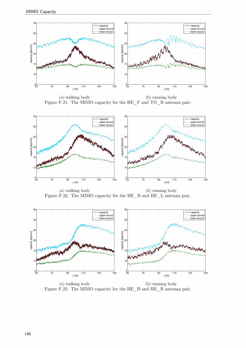
MIMO Capacity
50 70 90 110 130 1505
10
15
20
25
30
35
x [m]
capacity [bps/H
z]
capacity
upper bound
lower bound
50 70 90 110 130 1505
10
15
20
25
30
35
x [m]
capacity [bps/H
z]
capacity
upper bound
lower bound
(a) walking body (b) running bodyFigure F.21. The MIMO capacity for the HE_F and TO_B antenna pair.
50 70 90 110 130 1505
10
15
20
25
30
35
x [m]
capacity [bps/H
z]
capacity
upper bound
lower bound
50 70 90 110 130 1505
10
15
20
25
30
35
x [m]
capacity [bps/H
z]
capacity
upper bound
lower bound
(a) walking body (b) running bodyFigure F.22. The MIMO capacity for the HE_B and HE_L antenna pair.
50 70 90 110 130 1505
10
15
20
25
30
35
x [m]
capacity [bps/H
z]
capacity
upper bound
lower bound
50 70 90 110 130 1505
10
15
20
25
30
35
x [m]
capacity [bps/H
z]
capacity
upper bound
lower bound
(a) walking body (b) running bodyFigure F.23. The MIMO capacity for the HE_B and HE_R antenna pair.
146

Modelling MIMO Systems in Body Area Networks in Outdoors
50 70 90 110 130 1505
10
15
20
25
30
35
x [m]
capacity [bps/H
z]
capacity
upper bound
lower bound
50 70 90 110 130 1505
10
15
20
25
30
35
x [m]
capacity [bps/H
z]
capacity
upper bound
lower bound
(a) walking body (b) running bodyFigure F.24. The MIMO capacity for the HE_B and AB_L antenna pair.
50 70 90 110 130 1505
10
15
20
25
30
35
x [m]
capacity [bps/H
z]
capacity
upper bound
lower bound
50 70 90 110 130 1505
10
15
20
25
30
35
x [m]
capacity [bps/H
z]
capacity
upper bound
lower bound
(a) walking body (b) running bodyFigure F.25. The MIMO capacity for the HE_B and AB_R antenna pair.
50 70 90 110 130 1505
10
15
20
25
30
35
x [m]
capacity [bps/H
z]
capacity
upper bound
lower bound
50 70 90 110 130 1505
10
15
20
25
30
35
x [m]
capacity [bps/H
z]
capacity
upper bound
lower bound
(a) walking body (b) running bodyFigure F.26. The MIMO capacity for the HE_B and TO_B antenna pair.
147

MIMO Capacity
50 70 90 110 130 1505
10
15
20
25
30
35
x [m]
capacity [bps/H
z]
capacity
upper bound
lower bound
50 70 90 110 130 1505
10
15
20
25
30
35
x [m]
capacity [bps/H
z]
capacity
upper bound
lower bound
(a) walking body (b) running bodyFigure F.27. The MIMO capacity for the HE_L and HE_R antenna pair.
50 70 90 110 130 1505
10
15
20
25
30
35
x [m]
capacity [bps/H
z]
capacity
upper bound
lower bound
50 70 90 110 130 1505
10
15
20
25
30
35
x [m]
capacity [bps/H
z]
capacity
upper bound
lower bound
(a) walking body (b) running bodyFigure F.28. The MIMO capacity for the HE_L and AB_L antenna pair.
50 70 90 110 130 1505
10
15
20
25
30
35
x [m]
capacity [bps/H
z]
capacity
upper bound
lower bound
50 70 90 110 130 1505
10
15
20
25
30
35
x [m]
capacity [bps/H
z]
capacity
upper bound
lower bound
(a) walking body (b) running bodyFigure F.29. The MIMO capacity for the HE_L and AB_R antenna pair.
148

Modelling MIMO Systems in Body Area Networks in Outdoors
50 70 90 110 130 1505
10
15
20
25
30
35
x [m]
capacity [bps/H
z]
capacity
upper bound
lower bound
50 70 90 110 130 1505
10
15
20
25
30
35
x [m]
capacity [bps/H
z]
capacity
upper bound
lower bound
(a) walking body (b) running bodyFigure F.30. The MIMO capacity for the HE_L and TO_B antenna pair.
50 70 90 110 130 1505
10
15
20
25
30
35
x [m]
capacity [bps/H
z]
capacity
upper bound
lower bound
50 70 90 110 130 1505
10
15
20
25
30
35
x [m]
capacity [bps/H
z]
capacity
upper bound
lower bound
(a) walking body (b) running bodyFigure F.31. The MIMO capacity for the HE_R and AB_L antenna pair.
50 70 90 110 130 1505
10
15
20
25
30
35
x [m]
capacity [bps/H
z]
capacity
upper bound
lower bound
50 70 90 110 130 1505
10
15
20
25
30
35
x [m]
capacity [bps/H
z]
capacity
upper bound
lower bound
(a) walking body (b) running bodyFigure F.32. The MIMO capacity for the HE_R and AB_R antenna pair.
149

MIMO Capacity
50 70 90 110 130 1505
10
15
20
25
30
35
x [m]
capacity [bps/H
z]
capacity
upper bound
lower bound
50 70 90 110 130 1505
10
15
20
25
30
35
x [m]
capacity [bps/H
z]
capacity
upper bound
lower bound
(a) walking body (b) running bodyFigure F.33. The MIMO capacity for the HE_R and TO_B antenna pair.
50 70 90 110 130 1505
10
15
20
25
30
35
x [m]
capacity [bps/H
z]
capacity
upper bound
lower bound
50 70 90 110 130 1505
10
15
20
25
30
35
x [m]
capacity [bps/H
z]
capacity
upper bound
lower bound
(a) walking body (b) running bodyFigure F.34. The MIMO capacity for the AB_L and AB_R antenna pair.
50 70 90 110 130 1505
10
15
20
25
30
35
x [m]
capacity [bps/H
z]
capacity
upper bound
lower bound
50 70 90 110 130 1505
10
15
20
25
30
35
x [m]
capacity [bps/H
z]
capacity
upper bound
lower bound
(a) walking body (b) running bodyFigure F.35. The MIMO capacity for the AB_L and TO_B antenna pair.
150

Modelling MIMO Systems in Body Area Networks in Outdoors
50 70 90 110 130 1505
10
15
20
25
30
35
x [m]
capacity [bps/H
z]
capacity
upper bound
lower bound
50 70 90 110 130 1505
10
15
20
25
30
35
x [m]
capacity [bps/H
z]
capacity
upper bound
lower bound
(a) walking body (b) running bodyFigure F.36. The MIMO capacity for the AB_R and TO_B antenna pair.
The statistics of the capacity of 2×2 MIMO system, for the general antenna classes are presented
in Figure F.37.
F B L R FL FR BL BR FB LR10
15
20
25
capacity [bps/H
z]
F B L R FL FR BL BR FB LR10
15
20
25capacity [bps/H
z]
(a) walking body (b) running bodyFigure F.37. The capacity of 2×2 MIMO system, for the general antenna classes.
151

MIMO Capacity
The following tables includes the statistics of the MIMO capacity, and MIMO capacity channel
gain, for various pairs of antennas in 2×2 MIMO system, for the running body.
Table F.1. The capacity of 2×2 MIMO system, for TO_F & WA_F, for the running body.
x [m] CMIMO σCMIMOσCMIMO
GMIMOcσGMIMOc
σGMIMOc
[bps/Hz]
[50, 150] 16.41 6.23 2.21 1.45 0.17 0.17
[50, 85] 21.60 1.37 2.25 1.59 0.05 0.16
[85, 115] 19.40 4.02 2.34 1.53 0.09 0.17
[115, 150] 8.78 1.77 2.06 1.26 0.08 0.18
Table F.2. The capacity of 2×2 MIMO system, for TO_F & HE_F, for the running body.
x [m] CMIMO σCMIMOσCMIMO
GMIMOcσGMIMOc
σGMIMOc
[bps/Hz]
[50, 150] 17.29 6.23 2.17 1.51 0.17 0.16
[50, 85] 22.71 1.10 2.23 1.66 0.04 0.14
[85, 115] 19.98 4.05 2.28 1.59 0.08 0.16
[115, 150] 9.69 1.74 2.03 1.30 0.09 0.17
Table F.3. The capacity of 2×2 MIMO system, for TO_F & HE_B, for the running body.
x [m] CMIMO σCMIMOσCMIMO
GMIMOcσGMIMOc
σGMIMOc
[bps/Hz]
[50, 150] 16.15 2.71 1.44 1.18 0.17 0.10
[50, 85] 15.13 1.04 1.49 1.14 0.04 0.10
[85, 115] 19.60 2.14 1.86 1.38 0.18 0.14
[115, 150] 14.34 1.22 0.88 1.06 0.04 0.07
Table F.4. The capacity of 2×2 MIMO system, for TO_F & HE_L, for the running body.
x [m] CMIMO σCMIMOσCMIMO
GMIMOc σGMIMOcσGMIMOc
[bps/Hz]
[50, 150] 17.87 4.55 1.92 1.37 0.19 0.15
[50, 85] 20.35 2.00 2.16 1.53 0.10 0.16
[85, 115] 21.29 3.09 2.10 1.41 0.17 0.13
[115, 150] 12.61 1.86 1.45 1.18 0.06 0.14
152

Modelling MIMO Systems in Body Area Networks in Outdoors
Table F.5. The capacity of 2×2 MIMO system, for TO_F & HE_R, for the running body.
x [m] CMIMO σCMIMOσCMIMO
GMIMOcσGMIMOc
σGMIMOc
[bps/Hz]
[50, 150] 14.85 2.71 1.85 1.31 0.10 0.17
[50, 85] 16.62 0.94 1.82 1.25 0.04 0.14
[85, 115] 16.62 1.78 2.04 1.38 0.11 0.17
[115, 150] 11.67 1.25 1.72 1.31 0.10 0.19
Table F.6. The capacity of 2×2 MIMO system, for TO_F & AB_L, for the running body.
x [m] CMIMO σCMIMOσCMIMO
GMIMOcσGMIMOc
σGMIMOc
[bps/Hz]
[50, 150] 17.56 4.53 1.84 1.35 0.20 0.14
[50, 85] 19.56 2.74 2.02 1.47 0.19 0.14
[85, 115] 21.14 3.08 2.05 1.43 0.16 0.14
[115, 150] 12.64 2.04 1.42 1.17 0.08 0.14
Table F.7. The capacity of 2×2 MIMO system, for TO_F & AB_R, for the running body.
x [m] CMIMO σCMIMOσCMIMO
GMIMOcσGMIMOc
σGMIMOc
[bps/Hz]
[50, 150] 15.86 3.57 1.89 1.35 0.14 0.16
[50, 85] 17.84 1.95 1.94 1.35 0.11 0.15
[85, 115] 18.47 2.03 2.08 1.46 0.12 0.17
[115, 150] 11.77 1.66 1.68 1.26 0.12 0.17
Table F.8. The capacity of 2×2 MIMO system, for TO_F & TO_B, for the running body.
x [m] CMIMO σCMIMOσCMIMO
GMIMOcσGMIMOc
σGMIMOc
[bps/Hz]
[50, 150] 16.27 2.79 1.45 1.20 0.17 0.11
[50, 85] 15.48 1.51 1.45 1.17 0.07 0.11
[85, 115] 19.74 2.00 1.89 1.39 0.19 0.14
[115, 150] 14.22 1.24 0.94 1.07 0.05 0.07
153

MIMO Capacity
Table F.9. The capacity of 2×2 MIMO system, for WA_F & HE_F, for the running body.
x [m] CMIMO σCMIMOσCMIMO
GMIMOcσGMIMOc
σGMIMOc
[bps/Hz]
[50, 150] 17.38 6.25 2.13 1.52 0.17 0.16
[50, 85] 22.82 1.11 2.16 1.67 0.03 0.14
[85, 115] 20.12 4.02 2.25 1.60 0.08 0.16
[115, 150] 9.73 1.66 2.01 1.31 0.08 0.17
Table F.10. The capacity of 2×2 MIMO system, for WA_F & HE_B, for the running body.
x [m] CMIMO σCMIMOσCMIMO
GMIMOcσGMIMOc
σGMIMOc
[bps/Hz]
[50, 150] 16.20 2.68 1.47 1.18 0.17 0.11
[50, 85] 15.18 1.02 1.43 1.14 0.04 0.10
[85, 115] 19.67 2.09 1.94 1.38 0.18 0.14
[115, 150] 14.36 1.10 0.95 1.07 0.03 0.07
Table F.11. The capacity of 2×2 MIMO system, for WA_F & HE_L, for the running body.
x [m] CMIMO σCMIMOσCMIMO
GMIMOcσGMIMOc
σGMIMOc
[bps/Hz]
[50, 150] 17.98 4.55 1.93 1.37 0.19 0.15
[50, 85] 20.44 2.01 2.11 1.53 0.09 0.16
[85, 115] 21.46 3.05 2.11 1.42 0.17 0.13
[115, 150] 12.68 1.71 1.54 1.18 0.05 0.15
Table F.12. The capacity of 2×2 MIMO system, for WA_F & HE_R, for the running body.
x [m] CMIMO σCMIMOσCMIMO
GMIMOcσGMIMOc
σGMIMOc
[bps/Hz]
[50, 150] 14.92 2.67 1.85 1.31 0.10 0.17
[50, 85] 16.68 0.92 1.77 1.25 0.04 0.13
[85, 115] 16.68 1.74 2.07 1.38 0.11 0.17
[115, 150] 11.78 1.21 1.73 1.33 0.10 0.19
154

Modelling MIMO Systems in Body Area Networks in Outdoors
Table F.13. The capacity of 2×2 MIMO system, for WA_F & AB_L, for the running body.
x [m] CMIMO σCMIMOσCMIMO
GMIMOcσGMIMOc
σGMIMOc
[bps/Hz]
[50, 150] 17.66 4.55 1.87 1.36 0.20 0.14
[50, 85] 19.60 2.81 2.06 1.47 0.17 0.15
[85, 115] 21.36 3.01 2.06 1.46 0.17 0.14
[115, 150] 12.69 1.91 1.46 1.18 0.09 0.14
Table F.14. The capacity of 2×2 MIMO system, for WA_F & AB_R, for the running body.
x [m] CMIMO σCMIMOσCMIMO
GMIMOcσGMIMOc
σGMIMOc
[bps/Hz]
[50, 150] 15.98 3.63 1.90 1.36 0.15 0.16
[50, 85] 17.93 1.91 1.91 1.35 0.13 0.14
[85, 115] 18.67 2.21 2.10 1.48 0.11 0.16
[115, 150] 11.84 1.73 1.71 1.27 0.12 0.17
Table F.15. The capacity of 2×2 MIMO system, for WA_F & TO_B, for the running body.
x [m] CMIMO σCMIMOσCMIMO
GMIMOcσGMIMOc
σGMIMOc
[bps/Hz]
[50, 150] 16.32 2.80 1.50 1.20 0.17 0.11
[50, 85] 15.55 1.49 1.43 1.17 0.07 0.11
[85, 115] 19.80 2.11 1.98 1.39 0.18 0.14
[115, 150] 14.24 1.12 1.02 1.07 0.04 0.08
Table F.16. The capacity of 2×2 MIMO system, for HE_F & HE_B, for the running body.
x [m] CMIMO σCMIMOσCMIMO
GMIMOcσGMIMOc
σGMIMOc
[bps/Hz]
[50, 150] 16.32 2.59 1.51 1.19 0.16 0.11
[50, 85] 15.20 0.99 1.44 1.13 0.04 0.10
[85, 115] 19.64 2.07 1.90 1.37 0.18 0.14
[115, 150] 14.71 1.17 1.15 1.09 0.04 0.09
155

MIMO Capacity
Table F.17. The capacity of 2×2 MIMO system, for HE_F & HE_L, for the running body.
x [m] CMIMO σCMIMOσCMIMO
GMIMOcσGMIMOc
σGMIMOc
[bps/Hz]
[50, 150] 18.04 4.29 1.99 1.38 0.16 0.16
[50, 85] 20.09 2.13 2.07 1.50 0.10 0.16
[85, 115] 21.42 3.13 2.17 1.41 0.18 0.14
[115, 150] 13.25 1.76 1.74 1.24 0.06 0.17
Table F.18. The capacity of 2×2 MIMO system, for HE_F & HE_R, for the running body.
x [m] CMIMO σCMIMOσCMIMO
GMIMOcσGMIMOc
σGMIMOc
[bps/Hz]
[50, 150] 15.00 2.37 1.85 1.32 0.11 0.17
[50, 85] 16.37 1.08 1.72 1.22 0.04 0.13
[85, 115] 16.61 1.70 2.04 1.37 0.11 0.17
[115, 150] 12.36 1.19 1.82 1.39 0.09 0.19
Table F.19. The capacity of 2×2 MIMO system, for HE_F & AB_L, for the running body.
x [m] CMIMO σCMIMOσCMIMO
GMIMOcσGMIMOc
σGMIMOc
[bps/Hz]
[50, 150] 17.91 4.36 1.90 1.38 0.18 0.15
[50, 85] 19.70 2.75 2.06 1.46 0.17 0.15
[85, 115] 21.40 3.19 2.02 1.45 0.17 0.13
[115, 150] 13.29 1.85 1.61 1.24 0.10 0.16
Table F.20. The capacity of 2×2 MIMO system, for HE_F & AB_R, for the running body.
x [m] CMIMO σCMIMOσCMIMO
GMIMOcσGMIMOc
σGMIMOc
[bps/Hz]
[50, 150] 16.17 3.36 1.92 1.37 0.13 0.16
[50, 85] 17.94 1.91 1.90 1.34 0.12 0.14
[85, 115] 18.59 2.13 2.04 1.47 0.12 0.16
[115, 150] 12.45 1.70 1.83 1.33 0.11 0.18
156

Modelling MIMO Systems in Body Area Networks in Outdoors
Table F.21. The capacity of 2×2 MIMO system, for HE_F & TO_B, for the running body.
x [m] CMIMO σCMIMOσCMIMO
GMIMOcσGMIMOc
σGMIMOc
[bps/Hz]
[50, 150] 16.48 2.70 1.52 1.21 0.16 0.11
[50, 85] 15.58 1.48 1.45 1.16 0.07 0.11
[85, 115] 19.81 2.06 1.90 1.39 0.18 0.14
[115, 150] 14.64 1.16 1.19 1.10 0.04 0.10
Table F.22. The capacity of 2×2 MIMO system, for HE_B & HE_L, for the running body.
x [m] CMIMO σCMIMOσCMIMO
GMIMOcσGMIMOc
σGMIMOc
[bps/Hz]
[50, 150] 18.33 4.01 1.98 1.37 0.14 0.15
[50, 85] 14.20 1.43 1.74 1.26 0.05 0.16
[85, 115] 22.41 2.82 2.24 1.46 0.16 0.14
[115, 150] 19.11 2.34 1.96 1.42 0.11 0.15
Table F.23. The capacity of 2×2 MIMO system, for HE_B & HE_R, for the running body.
x [m] CMIMO σCMIMOσCMIMO
GMIMOcσGMIMOc
σGMIMOc
[bps/Hz]
[50, 150] 15.38 1.91 1.75 1.34 0.16 0.15
[50, 85] 13.27 1.27 1.85 1.46 0.08 0.18
[85, 115] 17.00 0.97 1.88 1.35 0.20 0.14
[115, 150] 16.21 0.88 1.52 1.21 0.03 0.12
Table F.24. The capacity of 2×2 MIMO system, for HE_B & AB_L, for the running body.
x [m] CMIMO σCMIMOσCMIMO
GMIMOcσGMIMOc
σGMIMOc
[bps/Hz]
[50, 150] 18.26 4.24 1.96 1.40 0.17 0.15
[50, 85] 13.88 1.62 1.72 1.29 0.11 0.16
[85, 115] 22.19 2.87 2.19 1.49 0.16 0.14
[115, 150] 19.42 2.89 1.98 1.44 0.18 0.15
157

MIMO Capacity
Table F.25. The capacity of 2×2 MIMO system, for HE_B & AB_R, for the running body.
x [m] CMIMO σCMIMOσCMIMO
GMIMOcσGMIMOc
σGMIMOc
[bps/Hz]
[50, 150] 16.57 3.15 1.87 1.38 0.16 0.15
[50, 85] 13.61 1.52 1.87 1.40 0.08 0.18
[85, 115] 19.20 2.24 2.08 1.48 0.16 0.15
[115, 150] 17.41 2.55 1.67 1.29 0.18 0.13
Table F.26. The capacity of 2×2 MIMO system, for HE_B & TO_B, for the running body.
x [m] CMIMO σCMIMOσCMIMO
GMIMOcσGMIMOc
σGMIMOc
[bps/Hz]
[50, 150] 18.44 5.65 2.13 1.55 0.14 0.16
[50, 85] 11.59 1.49 2.01 1.39 0.07 0.19
[85, 115] 21.49 3.91 2.28 1.63 0.07 0.15
[115, 150] 22.82 1.54 2.12 1.67 0.04 0.14
Table F.27. The capacity of 2×2 MIMO system, for HE_L & HE_R, for the running body.
x [m] CMIMO σCMIMOσCMIMO
GMIMOcσGMIMOc
σGMIMOc
[bps/Hz]
[50, 150] 16.35 1.39 1.79 1.36 0.14 0.16
[50, 85] 16.10 1.28 1.94 1.43 0.06 0.18
[85, 115] 17.59 0.95 1.72 1.17 0.06 0.12
[115, 150] 15.67 1.13 1.71 1.47 0.07 0.17
Table F.28. The capacity of 2×2 MIMO system, for HE_L & AB_L, for the running body.
x [m] CMIMO σCMIMOσCMIMO
GMIMOcσGMIMOc
σGMIMOc
[bps/Hz]
[50, 150] 19.56 3.84 2.09 1.53 0.08 0.16
[50, 85] 18.04 2.64 2.15 1.52 0.09 0.17
[85, 115] 24.13 2.03 2.15 1.58 0.06 0.13
[115, 150] 17.33 2.58 1.98 1.51 0.08 0.16
158
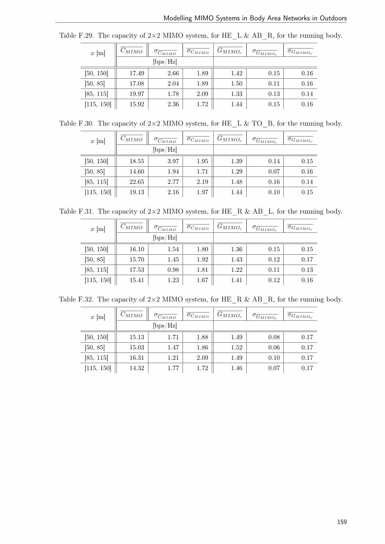
Modelling MIMO Systems in Body Area Networks in Outdoors
Table F.29. The capacity of 2×2 MIMO system, for HE_L & AB_R, for the running body.
x [m] CMIMO σCMIMOσCMIMO
GMIMOcσGMIMOc
σGMIMOc
[bps/Hz]
[50, 150] 17.49 2.66 1.89 1.42 0.15 0.16
[50, 85] 17.08 2.04 1.89 1.50 0.11 0.16
[85, 115] 19.97 1.78 2.09 1.33 0.13 0.14
[115, 150] 15.92 2.36 1.72 1.44 0.15 0.16
Table F.30. The capacity of 2×2 MIMO system, for HE_L & TO_B, for the running body.
x [m] CMIMO σCMIMOσCMIMO
GMIMOcσGMIMOc
σGMIMOc
[bps/Hz]
[50, 150] 18.55 3.97 1.95 1.39 0.14 0.15
[50, 85] 14.60 1.94 1.71 1.29 0.07 0.16
[85, 115] 22.65 2.77 2.19 1.48 0.16 0.14
[115, 150] 19.13 2.16 1.97 1.44 0.10 0.15
Table F.31. The capacity of 2×2 MIMO system, for HE_R & AB_L, for the running body.
x [m] CMIMO σCMIMOσCMIMO
GMIMOcσGMIMOc
σGMIMOc
[bps/Hz]
[50, 150] 16.10 1.54 1.80 1.36 0.15 0.15
[50, 85] 15.70 1.45 1.92 1.43 0.12 0.17
[85, 115] 17.53 0.98 1.81 1.22 0.11 0.13
[115, 150] 15.41 1.23 1.67 1.41 0.12 0.16
Table F.32. The capacity of 2×2 MIMO system, for HE_R & AB_R, for the running body.
x [m] CMIMO σCMIMOσCMIMO
GMIMOcσGMIMOc
σGMIMOc
[bps/Hz]
[50, 150] 15.13 1.71 1.88 1.49 0.08 0.17
[50, 85] 15.03 1.47 1.86 1.52 0.06 0.17
[85, 115] 16.31 1.21 2.09 1.49 0.10 0.17
[115, 150] 14.32 1.77 1.72 1.46 0.07 0.17
159
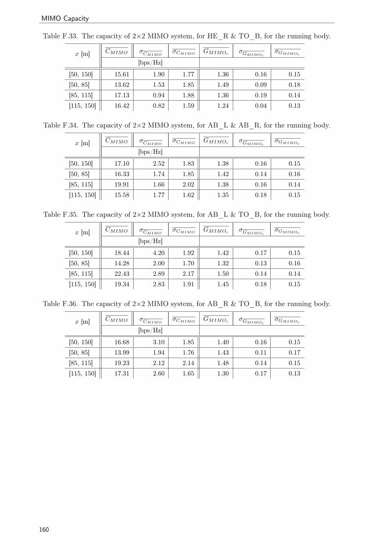
MIMO Capacity
Table F.33. The capacity of 2×2 MIMO system, for HE_R & TO_B, for the running body.
x [m] CMIMO σCMIMOσCMIMO
GMIMOcσGMIMOc
σGMIMOc
[bps/Hz]
[50, 150] 15.61 1.90 1.77 1.36 0.16 0.15
[50, 85] 13.62 1.53 1.85 1.49 0.09 0.18
[85, 115] 17.13 0.94 1.88 1.36 0.19 0.14
[115, 150] 16.42 0.82 1.59 1.24 0.04 0.13
Table F.34. The capacity of 2×2 MIMO system, for AB_L & AB_R, for the running body.
x [m] CMIMO σCMIMOσCMIMO
GMIMOcσGMIMOc
σGMIMOc
[bps/Hz]
[50, 150] 17.10 2.52 1.83 1.38 0.16 0.15
[50, 85] 16.33 1.74 1.85 1.42 0.14 0.16
[85, 115] 19.91 1.66 2.02 1.38 0.16 0.14
[115, 150] 15.58 1.77 1.62 1.35 0.18 0.15
Table F.35. The capacity of 2×2 MIMO system, for AB_L & TO_B, for the running body.
x [m] CMIMO σCMIMOσCMIMO
GMIMOcσGMIMOc
σGMIMOc
[bps/Hz]
[50, 150] 18.44 4.20 1.92 1.42 0.17 0.15
[50, 85] 14.28 2.00 1.70 1.32 0.13 0.16
[85, 115] 22.43 2.89 2.17 1.50 0.14 0.14
[115, 150] 19.34 2.83 1.91 1.45 0.18 0.15
Table F.36. The capacity of 2×2 MIMO system, for AB_R & TO_B, for the running body.
x [m] CMIMO σCMIMOσCMIMO
GMIMOcσGMIMOc
σGMIMOc
[bps/Hz]
[50, 150] 16.68 3.10 1.85 1.40 0.16 0.15
[50, 85] 13.99 1.94 1.76 1.43 0.11 0.17
[85, 115] 19.23 2.12 2.14 1.48 0.14 0.15
[115, 150] 17.31 2.60 1.65 1.30 0.17 0.13
160

Modelling MIMO Systems in Body Area Networks in Outdoors
Annex G. MIMO Performance
The capacity performance of 2×2 MIMO system, for the running body is presented in Figure G.1
and Figure G.2.
Figure G.1. The capacity performance of 2×2 MIMO system, for the running body (part 1).
161

MIMO Performance
Figure G.2. The capacity performance of 2×2 MIMO system, for the running body (part 2).
162

Modelling MIMO Systems in Body Area Networks in Outdoors
The capacity performance of 2×2 MIMO system, for the walking body is presented in Figure G.3
and Figure G.4.
Figure G.3. The capacity performance of 2×2 MIMO system, for the walking body (part 1).
163

MIMO Performance
Figure G.4. The capacity performance of 2×2 MIMO system, for the walking body (part 2).
164

Modelling MIMO Systems in Body Area Networks in Outdoors
References
[3GPP13] 3GPP - The 3rd Generation Partnership Project, http://www.3gpp.org, Feb.
2013.
[AAKC12] Ahn,C., Ahn,B., Kim,S. and Choi,J., "Experimental Outage Capacity Analysis
for Off-body Wireless Body Area Network Channel with Transmit Diversity",
IEEE Transactions on Consumer Electronics, Vol. 58, No. 2, May 2012, pp.
274-277.
[AIKT11] Aoyagi,T., Iswandi,I., Kim,M., Takada,J., Hamaguchi,K. and Kohno,R., "Body
Motion and Channel Response of Dynamic Body Area Channel", in Proc. of
EuCAP’2011 - 5th European Conference on Antennas and Propagation, Rome,
Italy, Apr. 2011.
[AKTH11] Aoyagi,T., Kim,M., Takada,J., Hamaguchi,K. and Kohno,R., "Numerical Si-
mulations for Dynamic WBAN Propagation Channel during Various Human
Movements", in Proc. of ISMICT’2011 - 5th International Symposium on
Medical Information and Communication Technology, Montreux, Switzerland,
Mar. 2011.
[ASAH09] Abbasi,Q., Sani,A., Alomainy,A. and Hao,Y., "Arm Movements Effect on Ultra
Wideband On-Body Propagation Channels and Radio Systems", in Proc. of
LAPC’2009 - Loughborough Antennas and Propagation Conference, Loughbo-
rough, UK, Nov. 2009.
[AlCS09] Ali,A.J., Cotton,S.L. and Scanlon,W.G., "Spatial Diversity for Off-Body Com-
munications in an Indoor Populated Environment at 5.8 GHz", in Proc. of
LAPC’2009 - Loughborough Antennas and Propagation Conference, Loughbo-
rough, UK, Nov. 2009.
[Asze96] Aszetly,D., On Antenna Arrays in Mobile Communication Systems: Fast Fa-
ding and GSM Base Station Receiver Algorithms, Ph.D. Thesis, Royal Institute
of Technology, Stockholm, Sweden, Mar. 1996.
[Bala05] Balanis,C.A., Antenna Theory, Analisys and Design, 3rd ed., John Wiley and
Sons, New York, NY, USA, 2005.
[Bala89] Balanis,C.A., Advanced Engineering Electromagnetics, John Wiley and Sons,
New York, NY, USA, 1989.
165

References
[CMAS12] Cotton,S.L., McKernan,A., Ali,A.J. and Scanlon,W.G., "An Experimental
Study on the Impact of Human Body Shadowing in Off-body Communications
Channels at 2.45 GHz", in Proc. of EuCAP’2012 - 6th European Conference
on Antenna and Propagation, Prague, Czech Republic, Apr. 2012.
[COST01] COST 259, http://info.grow.inov.pt/cost259, Dec. 2001.
[COST07] COST 273, http://info.grow.inov.pt/cost273, Dec. 2007.
[COST10] COST 2100, http://www.cost2100.org, Dec. 2010.
[COST13] COST IC1004, http://www.ic1004.org, Feb. 2013.
[COST89] COST 207, Digital Land Mobile Radio Communications, Final Report, COST
Telecom Secretariat, European Commision, Brussels, Belgium, 1989.
[COST99] COST 231, Digital Mobile Radio Towards Future Generation Systems, Final
Report, COST Telecom Secretariat, European Commision, Brussels, Belgium,
1999.
[CST12] CST - Computer Simulation Technology, http://www.cst.com, July 2012.
[ChCS09] Chandran,A.R., Conway,G.A. and Scanlon,W.G., "Pattern Switching Com-
pact Patch Antenna for On-body and Off-body Communications at 2.45 GHz",
in Proc. of EuCAP’2009 - 3rd European Conference on Antennas and Propa-
gation, Berlin, Germany, Mar. 2009.
[Chri10] Christ,A. et al, "The Virtual Family - Development of anatomical CAD models
of two adults and two children for dosimetric simulations", Physics in Medicine
and Biology, Vol. 55, No. 2, Jan. 2010, pp. 23-38.
[CoSc09] Cotton,S.L. and Scanlon,W.G., "Channel Characterization for Single- and
Multiple-Antenna Wearable Systems Used for Indoor Body-to-Body Commu-
nications", IEEE Transactions on Antennas and Propagation, Vol. 57, No. 4,
Apr. 2009, pp. 980-990.
[Corr01] Correia,L.M. (ed.), Wireless Flexible Personalised Communications, John Wi-
ley and Sons, Chichester, UK, 2001.
[Cube06] Cubero,S. (ed.), Industrial Robotics: Theory, Modelling and Control, Pro Li-
teratur Verlag, Vienna, Austria, 2006.
[Czin07] Czink,N., The Random-Cluster Model, Ph.D. Thesis, Technical University of
Vienna, Vienna, Austria, 2007.
166

Modelling MIMO Systems in Body Area Networks in Outdoors
[DCSZ10] Dai,H., Cai,B., Song,J. and Zhang,D., "Skeletal Animation Based on BVH
Motion Data", in Proc. of 2nd International Conference on Information En-
gineering and Computer Science, Wuhan, China, Dec. 2010.
[Dziu04] Dziunikowski,W., Multiple-Input Multiple-Output Antenna Systems, in Chan-
dran,S. (ed.), Adaptive Antenna Arrays, Springer, Berlin, Germany, 2004.
[ETSI13] ETSI - European Telecommunications Standards Institute,
http://www.etsi.org, Feb. 2013.
[ErOu10] Errico,R. and Ouvry,L., "A Statistical Model for On-Body Dynamic Chan-
nels", International Journal of Wireless Information Networks, Vol. 17, No.
3, Sep. 2010, pp. 92-104.
[FoGa98] Foschini,G.J. and Gans,M.J., "On Limits of Wireless Communications in a
Fading Environment when Using Multiple Antennas", Wireless Personal Com-
munication, Vol. 6, No. 3, Mar. 1998, pp. 311-335.
[GHBN11] Gallo,M., Hall,P.S., Bai,Q., Nechayev,Y.I., Constantinou,C.C. and Boz-
zetti,M., "Simulation and Measurement of Dynamic On-Body Communication
Channels", IEEE Transactions on Antennas and Propagation, Vol. 59, No. 2,
Feb. 2011, pp. 623-630.
[GaHB07] Gallo,M., Hall,P.S. and Bozzettil,M., "Use of Animation Software in the Si-
mulations of On-Body Communication Channels", in Proc. of LAPC’2007
- Loughborough Antennas and Propagation Conference, Loughborough, UK,
Apr. 2007.
[Gabr96] Gabriel,C., Compilation of Dielectric Properties of Body Tissues at
RF and Microwave Frequencies, Brooks Air Force Technical Report,
AL/OE-TR-1996-0037, San Antonio, TX, USA, 1996.
[Glas89] Glassner,A.S., An Introduction to Ray Tracing, Academic Press, New York,
NY, USA, 1989.
[GrNi96] Greenwood,P.E. and Nikulin,M.S., A Guide to Chi-squared Testing, John Wi-
ley and Sons, New York, NY, USA, 1996.
[HaHa06] Hall,P. and Hao,Y., Antennas and Propagation for Body-Centric Wireless
Communications, Artech House, Norwood, MA, USA, 2006.
[Hall07] Hall,P.S., "Antennas Challenges for Body Centric Communications", in Proc.
of IWAT’2007 - International Workshop on Antenna Technology: Small and
Smart Antennas Metamaterials and Applications, Cambridge, UK, Mar. 2007.
167

References
[HeUl09] Henneberg,M. and Ulijaszek,S., "Body Frame Dimensions are Related to Obe-
sity and Fatness: Lean Trunk Size, Skinfolds, and Body Mass Index", American
Journal of Human Biology, Vol. 22, No. 1, Apr. 2009, pp. 83-91.
[Hine96] Hines,J.W., "Medical and Surgical Applications of Space Biosensor Techno-
logy", Acta Astronautica, Vol. 38, No. 4-8, Feb./Apr. 1996, pp. 261-267.
[IEEE13a] IEEE 802, http://www.ieee802.org, Feb. 2013.
[IEEE13b] IEEE 802.15 Working Group for Wireless Personal Area Networks - Task
Group 6 (BAN), http://www.ieee802.org/15/pub/TG6.html, Feb. 2013.
[KHGN08] Khan,I., Hall,P., Guraliuc,A. and Nepa,P., "Reciprocity and Repeatability of
Diversity Measurements for On-Body Communication Channels at 2.45 GHz",
in Proc. of IEEE International Antennas and Propagation Symposium, San
Diego, CA, USA, July 2008.
[KTIV06] Krogerus,J., Toivanen,J., Icheln,C. and Vinikainen,P., "User Effect on Total
Radiated Power and 3D Radiation Pattern of Mobile Handsets", in Proc. of
EuCAP’2006 - 1st European Conference on Antennas and Propagation, Nice,
France, Nov. 2006.
[KhHa10] Khan,I. and Hall,P.S., "Experimental Evaluation of MIMO Capacity and Cor-
relation for Narrowband Body-Centric Wireless Channels", IEEE Transactions
on Antennas and Propagation, Vol. 58, No. 1, Jan. 2010, pp. 195-202.
[KmPN96] Knoblauch,R., Pietrucha,M. and Nitzburg,M., "Field Studies of Pedestrian
Walking Speed and Start-up Time", Transportation Research Record 1538,
Transportation Research Board, National Research Council, Washington, DC,
USA, 1996, pp. 27-38.
[Kosi04] Kosilo,T., Mobile Terrestial Radiocommunications (in Polish), Internal Docu-
ment, Warsaw University of Technology, Warsaw, Poland, 2004.
[Kuma80] Kumaraswamy,P., "A Generalized Probability Density Function for
Double-bounded Random Processes", Journal of Hydrology, Vol. 46, No. 1-2,
Mar. 1980, pp. 79-88.
[LEXN13] LEXNET - Low EMF Exposure Future Networks,
http://grow.inov.pt/projects/lexnet, Feb. 2013.
[LKCD11] Liu,L., Keshmiri,F., Craeye,C., Doncker,P. and Oestges,C., "An Analytical
Modeling of Polarized Time-Variant On-Body Propagation Channels with Dy-
namic Body Scattering", EURASIP Journal on Wireless Communications and
Networking, Vol. 2011, Apr. 2011.
168

Modelling MIMO Systems in Body Area Networks in Outdoors
[LRDO09] Liu,L., Roy,S., Doncker,P. and Oestges,C., "Azimuth Radiation Pattern Cha-
racterization of Omnidirectional Antennas Near a Human Body", in Proc. of
ICEAA’2009 - 11th International Conference on Electromagnetics in Advanced
Applications, Torino, Italy, Sep. 2009.
[LaFL12] Langley,R.J., Ford,K.L. and Lee,H.J., "Switchable On/Off-body Communica-
tion at 2.45 GHz Using Textile Microstrip Patch Antenna on Stripline", in
Proc. of EuCAP’2012 - 6th European Conference on Antennas and Propaga-
tion, Prague, Czech Republic, Mar. 2012.
[LiRa99] Liberti,J. and Rappaport,T., Smart Antennas for Wireless Communication:
IS-95 and Third Generation CDMA Applications, Prentice Hall, Upper Saddle
River, NJ, USA, 1999.
[MCCF07] Medeiros,C.R., Castela,A.M., Costa,J.R. and Fernandes,C.A., "Evaluation of
Modelling Accuracy of Reconfigurable Patch Antennas", in Proc. of ConfTele
- Conference on Telecommunications, Peniche, Portugal, May 2007.
[MOLC11] Mackowiak,M., Oliveira,C., Lopes,C.G. and Correia,L.M., "A Statistical Ana-
lysis of the Influence of the Human Body on the Radiation Pattern of Wearable
Antennas", in Proc. of PIMRC’2011 - 22nd IEEE International Symposium on
Personal, Indoor and Mobile Radio Communications, Toronto, Canada, Sep.
2011.
[MREC13] Mackowiak,M., Rosini,R., Errico,R. and Correia,L.M., "Comparing Off-Body
Dynamic Channel Model with Real-Time Measurements", in Proc. of
ISMICT’2013 - 7th International Symposium on Medical Information and
Communication Technology, Tokyo, Japan, Mar. 2013.
[MaCo04] Marques,M.G. and Correia,L.M., A Wideband Directional Channel Model for
Mobile Communication Systems, in Chandran,S. (ed.), Adaptive Antenna Ar-
rays, Springer, Berlin, Germany, 2004.
[MaCo10] Mackowiak,M. and Correia,L.M., "A Statistical Approach to Model Antenna
Radiation Patterns in Off-Body Radio Channels", in Proc. of PIMRC’2010
- 21st IEEE International Symposium on Personal, Indoor and Mobile Radio
Communications, Istanbul, Turkey, Sep. 2010.
[MaCo11] Mackowiak,M. and Correia,L.M., "Modelling the Influence of Body Dynamics
on the Radiation Pattern of Wearable Antennas in Off-Body Radio Channels",
in Proc. of 12th URSI Commission F Triennial Open Symposium on Radio
Wave Propagation and Remote Sensing, Garmisch-Partenkirchen, Germany,
Mar. 2011.
169

References
[MaCo12b] Mackowiak,M. and Correia,L.M., "Correlation Analysis in Off-Body Radio
Channels in a Street Environment", in Proc. of PIMRC’2012 - 23rd IEEE
Symposium on Personal, Indoor, Mobile and Radio Communications, Sydney,
Australia, Sep. 2012.
[MaCo12c] Mackowiak,M. and Correia,L.M., "Towards a Radio Channel Model for
Off-Body Communications in a Multipath Environment", in Proc. of EW’2012
- 18th European Wireless Conference, Poznan, Poland, Apr. 2012.
[MaCo13a] Mackowiak,M. and Correia,L.M., "A Statistical Model for the Influ-
ence of Body Dynamics on the Radiation Pattern of Wearable Anten-
nas in Off-Body Radio Channels", Wireless Personal Communications,
10.1007/s11277-013-1193-x, May 2013
[MaCo13b] Mackowiak,M. and Correia,L.M., "MIMO Capacity Analysis of Off-Body Ra-
dio Channels in a Street Environment", in Proc. of VTC’2013 Spring - IEEE
77th Vehicular Technology Conference, Dresden, Germany, June 2013.
[MaCo13c] Mackowiak,M. and Correia,L.M., "MIMO Capacity Performance of Off-Body
Radio Channels in a Street Environment", accepted to PIMRC’2013 - 24th
IEEE Symposium on Personal, Indoor, Mobile and Radio Communications,
London, UK, Sep. 2013.
[MaMy78] Macomber,J.H. and Myers,B.L., "The Bivariate Beta Distribution: Compari-
son of Monte Carlo Generators and Evaluation of Parameter Estimates", in
Proc. of 10th Conference on Winter Simulation, Miami Beach, FL, USA, Jan.
1978.
[MaOC12a] Mackowiak,M., Oliveira,C. and Correia,L.M., "Radiation Pattern of Wearable
Antennas: A Statistical Analysis of the Influence of the Human Body", Inter-
national Journal of Wireless Information Networks, Vol. 19, No. 3, Sep. 2012,
pp. 209-218.
[MaOC12b] Mackowiak,M., Oliveira,C. and Correia,L.M., "Signal Correlation Between We-
arable Antennas in Body Area Networks in Multipath Environment", in Proc.
of EuCAP’2012 - 6th European Conference on Antennas and Propagation, Pra-
gue, Czech Republic, Mar. 2012.
[Mack07] Mackowiak,M., Geometrically Based Multibounce MIMO Channel Model, M.Sc.
Thesis, IST-TUL, Lisbon, Portugal, 2007.
[Moli05] Molisch,A.F., Wireless Communications, Wiley-IEEE Press, West Sussex, UK,
2006.
170

Modelling MIMO Systems in Body Area Networks in Outdoors
[NEWC11] NEWCOM++ - Network of Excellence in Wireless Communications,
http://130.192.85.4:8080/Plone, Dec. 2011.
[NEWC13] NEWCOM# - Network of Excellence in Wireless Communications,
http://www.newcom-project.eu, Feb. 2013.
[NaHH10] Nechayev,Y., Hu,Z.H. and Hall,P., "Fading of the Transmission Channel be-
tween two Wireless Body Area Networks in an Office at 2.45 GHz and 5.8 GHz",
in Proc. of LAPC’2010 - Loughborough Antennas and Propagation Conference,
Loughborough, UK, Nov. 2010.
[OMLC11] Oliveira,C., Mackowiak,M., Lopes,C.G. and Correia,L.M., "Characterisation of
On-Body Communications at 2.45 GHz", in Proc. of BodyNets - International
Conference on Body Area Networks, Beijing, China, Nov. 2011.
[OgHo12] Ogawa,K. and Honda,K., "BAN Shadowing Properties of an Arm-Waving Dy-
namic Phantom", in Proc. of EuCAP’2012 - 6th European Conference on
Antennas and Propagation, Prague, Czech Republic, Mar. 2012.
[OlMC11] Oliveira,C., Mackowiak,M. and Correia,L.M., "Challenges for Body Area Ne-
tworks Concerning Radio Aspects", in Proc. EW’2011 - 17th European Wire-
less Conference, Vienna, Austria, Apr. 2011.
[OlMC12a] Oliveira,C., Mackowiak,M. and Correia,L.M., Statistical Characterisation of
Antennas in BANs, in Guillaume de la Roche, Andres Alayon-Glazunov and
Ben Allen (eds.), LTE Advanced and Beyond Wireless Networks: Channel Mo-
delling and Propagation, John Wiley, Chichester, UK, 2012.
[OlMC12b] Oliveira,C., Mackowiak,M. and Correia,L.M., "A Comparison of Phantom Mo-
dels for On-Body Communications", in Proc. of PIMRC’2012 - 23rd IEEE
Symposium on Personal, Indoor, Mobile and Radio Communications, Sydney,
Australia, Sep. 2012.
[OlMC12c] Oliveira,C., Mackowiak,M. and Correia,L.M., "Correlation Analysis in
On-Body Communications", in Proc. of EuCAP’2012 - 6th European Con-
ference on Antennas and Propagation, Prague, Czech Republic, Mar. 2012.
[OlMC13] Oliveira,C., Mackowiak,M. and Correia,L.M., "Modelling On- and Off-Body
Channels in Body Area Networks", invited to IMOC’2013 - International Mi-
crowave and Optoelectronics Conference, Rio de Janeiro, Brazil, Aug. 2013.
[Orfa96] Orfanidis,S.J., An Introduction to Optimum Signal Processing, Prentice-Hall,
Englewood Cliffs, NJ, USA, 1996.
[POSE12] POSER, http://poser.smithmicro.com, Dec. 2012.
171

References
[PaJa03] Park,S. and Jayaraman,S., "Enhancing the Quality of Life Through Wearable
Technology", IEEE Engineering in Medicine and Biology Magazine, Vol. 22,
No. 3, May/June 2003, pp. 41-48.
[Path82] Pathak,P.H., "Uniform Geometrical Theory of Diffraction", in Proc. of Appli-
cations of Mathematics in Modern Optics, San Diego, CA, USA, Aug. 1982.
[Proa01] Proakis,J.G., Digital Communications, Mac Graw Hill, New York, NY, USA,
2001.
[RoEr12] Rosini,R. and Errico,R., "Off-Body Channel Modelling at 2.45 GHz for Two
Different Antennas", in Proc. of EuCAP’2012 - 6th European Conference on
Antennas and Propagation, Prague, Czech Republic, Mar. 2012.
[SBMS04] Schumacher,L., Berger,L.T., Ramiro-Moreno,J. and Sorensen,T.B., Propaga-
tion Characterization and MIMO Channel Modelling for 3G, in Chandran,S.
(ed.), Adaptive Antenna Arrays, Springer, Berlin, Germany, 2004.
[SCAD12] SEMCAD, http://www.speag.com/products/semcad/overview, Dec. 2012.
[SHZM09] Smith,D., Hanlen,L.W., Zhang,J.A., Miniutti,D., Rodda,D. and Gilbert,B.,
"Characterization of the Dynamic Narrowband On-Body to Off-Body Area
Channel", in Proc. of ICC’2009 - IEEE International Conference on Commu-
nications, Dresden, Germany, June 2009.
[SJKM03] Sarkar,T.K, Ji,Z., Kim,K., Medouri,A. and Salazar-Palma,M., "A Survey of
Various Propagation Models for Mobile Communication", IEEE Antennas and
Propagation Magazine, Vol. 45, No. 3, June 2003, pp. 51-82.
[SaVa87] Saleh,A.M. and Valenzuela,R.A., "A Statistical Model for Indoor Multipath
Propagation", IEEE Journal on Selected Areas in Communications, Vol. 5,
No. 2, Feb. 1987, pp. 128-137.
[Sadi00] Sadiku,M., Numerical Techniques in Electromagnetics, CRC Press, Prairie
View, TX, USA, 2000.
[Sibi08] Sibille,A., "Statistical Antenna Modeling", in Proc. of URSI - 29th General
Assembly, Chicago, IL, USA, Aug. 2008.
[Skla97] Sklar,B., "Rayleigh Fading Channels in Mobile Digital Communication Sys-
tems. Part I", IEEE Communications Magazine, Vol. 35, No. 9, July 1997,
pp. 136-146.
172

Modelling MIMO Systems in Body Area Networks in Outdoors
[SmHL11] Smith,D., Hanlen,L.W. and Lamahewa,T.A., "A New Look at the Body Area
Network Channel Model", in Proc. of EuCAP’2011 - 5th European Conference
on Antennas and Propagation, Rome, Italy, Apr. 2011.
[TaKi06] Tavakol,V. and Kildal,P.S., "Relations between Radiation Characteristics of
Small Antennas Located in Free Space and Close to Lossy Phantom", in Proc.
of IEEE Antennas and Propagation Society International Symposium, Albu-
querque, NM, USA, July 2006.
[Tela95] Telatar,I.E., Capacity of Multi-Antenna Gaussian Channels, ATT Bell
Labs, Technical memorandum BL011217-950615-07TM, NJ, USA, June 1995,
(http://www.bell-labs.com/org/physicalsciences/pubs/lozano.pdf).
[VPop12] Virtual Population, http://www.itis.ethz.ch/services/anatomical-models, Dec.
2012.
[VTHR10] Vallozzi,L., Torre,P., Hertleer,C., Rogier,H., Moeneclaey,M. and Verhaevert,J.,
"Wireless Communication for Firefighters Using Dual-Polarized Textile An-
tennas Integrated in Their Garment", IEEE Transactions on Antennas and
Propagation, Vol. 58, No. 4, Apr. 2010, pp. 1357-1368.
[VaAn87] Vaughan,R. and Andersen,J., "Antenna Diversity in Mobile Communications",
IEEE Transactions Vehicular Technology, Vol. 36, No. 4, Nov. 1987, pp.
149-172.
[YSKO11] Yamamoto,N., Shirakata,N., Kobayashi,D. and Ogawa,K., "BAN Communi-
cation Quality Assessments Using an Arm-Waving Dynamic Phantom Re-
plicating the Walking Motion of a Human", in Proc. of ICC’2011 - IEEE
International Conference on Communications, Kyoto, Japan, June 2011.
173