modelling of electromechanical control of camless internal ... · modelling of electromechanical...

123

International Journal of

Science and Engineering Investigations vol. 2, issue 15, April 2013

ISSN: 2251-8843

Modelling of Electromechanical Control of Camless Internal

Combustion Engine Valve Actuator

Jeremiah L. Chukwuneke1, Chinonso H. Achebe

2, Paul C. Okolie

3, Obiora E. Anisiji

4

1,2,3Department of Mechanical Engineering, Nnamdi Azikiwe University, Awka, Anambra State, Nigeria

4Department of Engineering Research Development and Production, Projects Development Institute, Enugu, Nigeria

([email protected])

Abstract- This paper presents the modeling and control of internal combustion engine valve actuator mechanism, using variable valve actuation system, like electromechanical valve actuation system to flexibly control the engine valve timing and lift profile. In this paper, the prospects and possibilities of an electromechanical control of internal combustion engine valve to eliminate choking and backflow has been theoretically and technically analyzed. In principle, optimality in every engine condition can be attained by Camless valve trains. Electromechanical valve actuators are very promising in this context. A mathematical model of the system is developed to evaluate the effect of each of the design parameters, starting from the modeling of a single stage pressure reducing valve, the concept of modeling a real three land three way solenoid valve actuator for the clutch system in the automatic transmission is presented and these were validated with data provided from experiments with the real valve actuator on a test bench. A simulator in a Matlab for an input-output model is developed and significant improvements in fuel economy, engine performance, efficiency, maximum torque and power, pollutant emissions were achieved. A position feedback closed-loop controller that reduced the valve landing velocity from 0.55m/s to 0.16m/s with consistent transition time of 3.42ms were designed in a Matlab Simulink and implemented.

Keywords- Internal Combustion Engine, Electromechanical

Valve, Camless, Variable Valve Timing, Control, Actuator,

Armature.

I. INTRODUCTION

Internal combustion engines traditionally use mechanically driven camshaft to actuate intake and exhaust valves. Their lift’s profiles are direct function of the shape of the cam (engine crank angle) and cannot be adjusted to optimize engine performances in different operating conditions. This fact results in a compromise design that impacts on achievable engine efficiency, maximum torque and power, and pollutant emission.

Growing needs to improve fuel economy and reduce exhaust emissions lead to the development of alternative valve

operating methods, which aim to alleviate or completely avoid the limitations imposed by fixed valve timing.

To fully exploit the possibilities offered by a complete Variable Valve Timing (VVT) system, camless engine valve trains, in which the valve motion is completely independent of the piston motion, are currently the topic of an intensive research activity, both from academia and several manufacturers. This paper focuses on an electromechanical valve actuator [1][2] for camless engines.

Despite the cited advantages, use of electromechanical actuators has been delayed by significant control problems that are still open [3][4][1] and by significant system costs. The biggest control difficulty comes from the valve seating velocity, i.e. the valve velocity when it comes against the closing position. It should be very low to avoid acoustical noise and wear and tear of mechanical components, with typical values between 0.05 m/s and 0.1 m/s at idle speed [5].

It is highly desired that an ICE valve fully opens or closes instantaneously so that choking flow, which reduces the volumetric efficiency, can be eliminated. But the shape of the cam which would satisfy or approach to an appreciable degree of satisfying such a lift profile would suffer from loss of contact (separation), which is a situation where the cam follower finds it difficult catching up with the cam thereby loses contact with the cam, and problems associated with vibration occurs. This is the reason the valves actuated by cam mechanism are gradually opened and closed. One of the precautions or design considerations to be taken while designing an electromechanical valve control is the prevention of instantaneously opening the valve when the piston head is fast approaching the top-dead-center. The working principle of an electromechanical valve actuator proposed in this work is briefly described below.

An electromechanical actuator for an internal combustion engine valve comprises electromagnets and springs for controlling the position of the valve by means of electric signals. When current flows in the coil of the upper electromagnet, the latter is activated and generates a magnetic field attracting the plate (also called armature), which comes into contact with it. The simultaneous displacement of the rod enables the spring to bring the valve into the closed position, the head of the valve coming into contact with the seat and

International Journal of Science and Engineering Investigations, Volume 2, Issue 15, April 2013 124

www.IJSEI.com Paper ID: 21513-22 ISSN: 2251-8843

preventing the exchange of gas between the interior and exterior of the cylinder [6].

Analogously, when current flows in the coil of lower electromagnet, the upper electromagnet brings deactivation, it is activated and attracts the armature, which comes into contact with it and displaces the rod by means of the spring in such a way that this rod acts on the valve and brings the latter into the open position, the head of the valve being moved away from its seat to permit the admission or the injection of gas into the cylinder [6].

Electro-Mechanical Valve (EMV) actuators shown in Fig.1 (a) & (b) are currently being developed by many engine and component manufacturers. These actuators can potentially improve engine performance via flexibility in valves timings at all engine operating conditions. Unlike conventional camshaft driven systems, EMV system affords valve timings that are fully independent of crankshaft position. The additional

flexibility in valve timing gives excellent cycle-to-cycle control of cylinder air charge and residual gas fractions. Fuel economy can be improved through un-throttled load control and cylinder deactivation. Internal residuals together with appropriate valve actuation schemes can be used to lower exhaust emissions below engines with a camshaft. At low-to moderate engine speeds, valve timings can be optimized to improve full load torque.

Although a conventional valve train system limits engine performance, it has operational advantages. The valve motion is controlled by a cam profile that is carefully designed to give low seating velocities for durability and low noise. In contrast, an EMV system introduces a difficult motion control problem. Accurate valve timings, fast transitions, and low seating velocities (soft landing) must be achieved. Robust soft landing control is required before EMV systems are introduced into the market.

(a)

(b)

Figure 1. (a) Sketch of electromechanical valve actuator. (b) EMV actuator assembly with valve shown in open position



This type of system uses an armature attached to the valve stem. The outside casing contains a magnetic coil of some sort that can be used to either attract or repel the armature, hence opening or closing the valve.

Most early systems employed solenoid and magnetic attraction/repulsion actuating principals using an iron or ferromagnetic armature [7]. These types of armatures limited the performance of the actuator because they resulted in a variable air gap. As the air gap becomes larger (i.e. when the distance between the moving and stationary magnets or electromagnets increases), there is a reduction in the force. To maintain high forces on the armature as the size of the air gap increases, a higher current is employed in the coils of such devices. This increased current leads to higher energy losses in the system, not to mention non-linear behaviour that makes it difficult to obtain adequate performance. The result of this is that most such designs have high seating velocities (i.e. the valves slam open and shut hard!) and the system cannot vary the amount of valve lift [8].

The electromechanical valve actuators of the latest poppet valve design eliminate the iron or ferromagnetic armature. Instead it is replaced with a current-carrying armature coil. A magnetic field is generated by a magnetic field generator and is directed across the fixed air gap. An armature having a current-carrying armature coil is exposed to the magnetic field in the air gap. When a current is passed through the armature coil and that current is perpendicular to the magnetic field, a force is exerted on the armature. When a current runs through the armature coil in both direction and perpendicular to the magnetic field, an electromagnetic vector force, known as a Lorentz force, is exerted on the armature coil. The force generated on the armature coil drives the armature coil linearly in the air gap in a direction parallel with the valve stem. Depending on the direction of the current supplied to the armature coil, the valve will be driven toward an open or closed position [8]. These latest electromechanical valve actuators develop higher and better-controlled forces than those designs mentioned previously. These forces are constant along the distance of travel of the armature because the size of the air gap does not change.

II. THEORETICAL CONSIDERATION

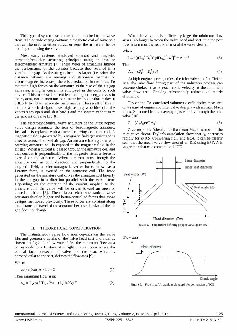
The instantaneous valve flow area depends on the valve lifts and geometric details of the valve head seat and stem as shown on fig.2. For low valve lifts, the minimum flow area corresponds to a frustum of a right circular cone where the conical face between the valve and the seat, which is perpendicular to the seat, defines the flow area [9];

When:

w/(sinβcosβ) > Lv > O (1)

Then minimum flow area;

Am = Lvcosβ[Dv - 2w + (Lvsin2β)/2] (2)

When the valve lift is sufficiently large, the minimum flow area is no longer between the valve head and seat, it is the port flow area minus the sectional area of the valve steam;

When

Lv > [((Dp2-Ds

2)/ (4Dm))

2-w

2]

½ + wtanβ (3)

Then

Am = ( /4 (4)

At high engine speeds, unless the inlet valve is of sufficient size, the inlet flow during part of the induction process can become choked, that is reach sonic velocity at the minimum valve flow area. Choking substantially reduces volumetric efficiency.

Taylor and Co. correlated volumetric efficiencies measured on a range of engine and inlet valve designs with an inlet Mach index, Z, formed from an average gas velocity through the inlet valve [10].

Z = (ApSp)/(CiAia) (5)

Z corresponds “closely” to the mean Mach number in the inlet valve throat. Taylor’s correlation show that ηv decreases rapidly for Z≥0.5. Comparing fig.3 and fig.4, it can be clearly seen that the mean valve flow area of an ICE using EMVA is larger than that of a conventional ICE.

Figure 2. Parameters defining poppet valve geometry

Figure 3. Flow area Vs crank angle graph for convention of ICE



Figure 4. Predicted flow area Vs crank angle graph for ICE using EMVA

The slope of the line joining the maximum flow area and zero is very steep because the valve which is electromechanically controlled opens and closes fully very fast almost instantaneously. The drop in pressure along the intake system depends on engine speed, the flow resistance of the elements in the system, the cross-sectional area through which the fresh change moves, and the change density. The usual practice is extending the valve open phases beyond the intake and exhaust strokes to improve emptying and charging of the cylinders and make the best use of the inertia of the gases in the intake and exhaust system.

Typically, the exhaust valve closes 150 to 30

0 after TC and

inlet valve opens 100 to 20

0 before TC, both valves are open

during overlap period. The advantage of valve overlap occurs at high engine speed when the longer valve-open periods improve volumetric efficiency. An assumed situation where the valve overlap period can be varied with respect to the engine speed in an ICE using EMVA came up with graphs shown in fig.7. The dotted line is lift profile at low engine speed. From the graph in fig.7; valve overlap period is longer at higher engine speed. A proposed longer period of valve overlap of rams and turning effects can be fully utilized, since at higher engine speeds, the inertia of the gas in the intake system (as the intake valve is closing) increases the pressure in the port, but the period of the reverse flow into the intake (back flow). It is predicted that ηv versus N graph for a varying valve turning (including varying valve overlap) looks like fig.8 (a) because the turning and ram effects will be fully utilized, choking effect will be eliminated or greatly reduced so also will back flow effects be greatly reduced.

Figure 5. Valve Timing diagram for typical ICE

Figure 6. Valve lift Vs crank angle for typical ICE

Figure 7. Valve lift Vs crank angle for a varying timing at both high and low

engine speeds

(a)

(b)

Figure 8. (a) ηv versus N for typical ICE. (b) ηv versus N for ICE using

variable valve timing



III. MATHEMATICAL MODEL FOR THE SYSTEM

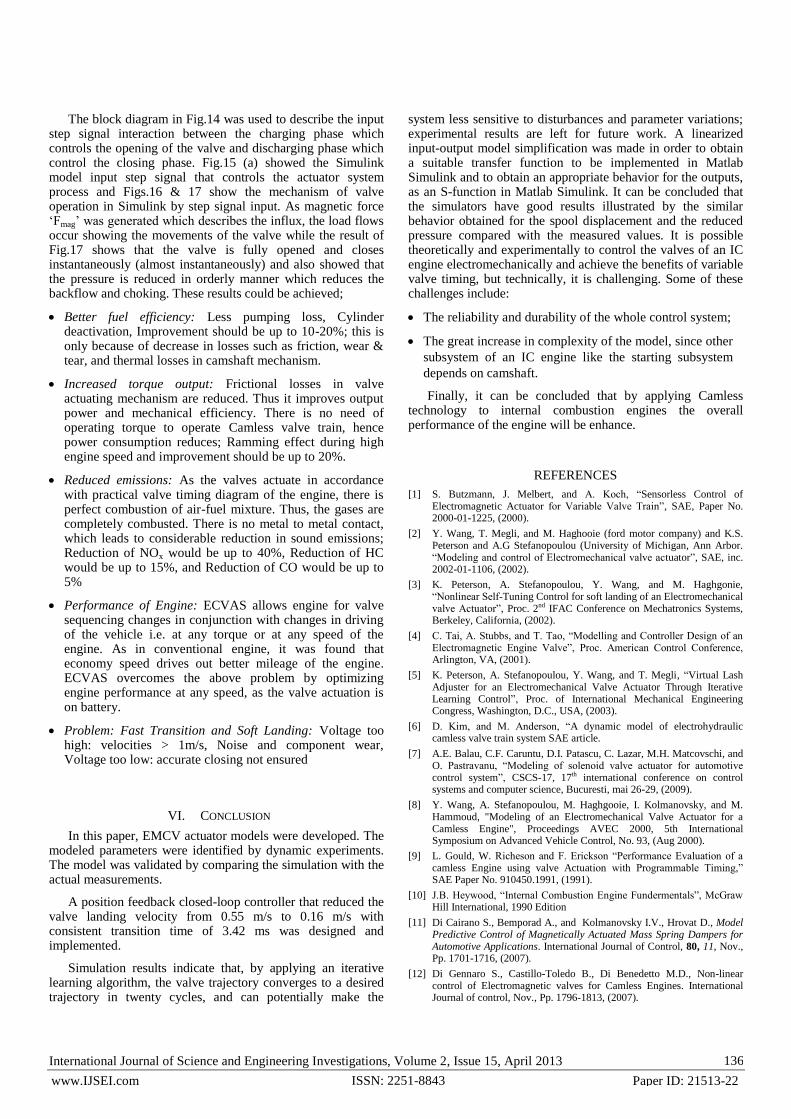
Figure 1(b) shows a schematic of an EMV actuator mounted on a cylinder head. The actuator consists of a lower electromagnetic coil for opening the valve and an upper coil for closing the valve. Actuator and valve springs push on the armature and valve stem through spring retainers. At neutral position the actuator and valve springs are equally compressed and the armature is centered between the upper and lower coils. At start-up, a voltage is applied to one of the electromagnets to move the armature from neutral position to the fully open or fully closed position. A small holding voltage is then maintained to hold the armature in place against the spring force.

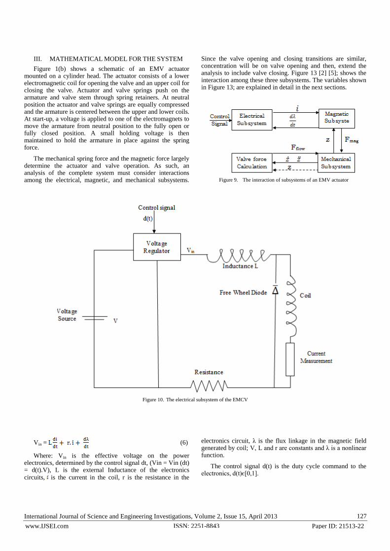
The mechanical spring force and the magnetic force largely determine the actuator and valve operation. As such, an analysis of the complete system must consider interactions among the electrical, magnetic, and mechanical subsystems.

Since the valve opening and closing transitions are similar, concentration will be on valve opening and then, extend the analysis to include valve closing. Figure 13 [2] [5]; shows the interaction among these three subsystems. The variables shown in Figure 13; are explained in detail in the next sections.

Figure 9. The interaction of subsystems of an EMV actuator

Figure 10. The electrical subsystem of the EMCV

Vin = (6)

Where: Vin is the effective voltage on the power electronics, determined by the control signal dt, (Vin = Vin (dt) = d(t).V), L is the external Inductance of the electronics circuits, is the current in the coil, r is the resistance in the

electronics circuit, λ is the flux linkage in the magnetic field generated by coil; V, L and r are constants and λ is a nonlinear function.

The control signal d(t) is the duty cycle command to the electronics, d(t)є[0,1].



Consider the operation described for valve opening in fig.10; the following d(t) for the lower credit in operation cycle.

d(t) = (7)

Fig.11; shows the mechanical subsystem and the associated force body diagram when the valve is at the middle position.

The moving mass of the mechanical system includes three parts: the upper spring bolt, the armature, and the valve with the valve spring bolt.

In this paper, lumping was considered for all the three pieces in one mass because they are moving together during most of the travel from one coil to another. Fig.11; shows the spring forces from the actuator spring (Fus) and the valve spring (Fℓs) and the magnetic force (Fmag). Also shown are the damping force inside the actuator (Fdamp) and the gas flow force (Fflow) on the valve.

Figure 11. The Mechanical Subsystem of the EMCV

The differential equation describing the one mass spring mechanical subsystem is given by the Newton’s law,

M (8)

Where; M is the mass of the moving parts in the actuator, z is the distance between the armature and the lower coil, z є (0,8)mm, when z = 0, the armature contacts the lower coil and the valve is in the open position, when z = 8mm, the armature contacts the upper coil and the valve is in the closed position, Fmag is the magnetic force generated by the coil, Fus is the spring force from the upper spring, Fls is the spring force from the lower spring, Fdamp is the damping force inside the actuator due to the friction, Fflow is the gas flow force on the valve generated when the valve separated chambers have different pressures.

The positive direction for the forces is in the direction of increasing distance z. In calculation of the spring force Fus and Fℓs, (assume linear springs). This assumption was tested by measuring the spring force for different spring compression. From the measurement, the spring constant was identified as Ks = 75N/mm for both springs.

Therefore, the following spring forces were generated:

Fus = Ks(Zs + z – 4) = Ks(z-4) + KsZs (9)

Fℓs = Ks(Zs + 4 - z) = Ks(4 - z) + KsZs (10)

Where, Zs is the initial compression of both springs at the equilibrium point (z = 4mm). Consequently,

Fℓs – Fus = 2.ks(4 – z). Here, it was noticed that to satisfy the requirement that both springs are compressed during the whole travel of the armature (Fℓs and Fus are both positive when zє[0,8]mm), it is required that zs>4mm.

Then;

Fflow = (Pcyl x Acyl) – (Pexh x Aev) (11)

Where; Aev, Acyl are the area of the exhaust valve and cylinder respectively. When the valve starts opening, there is no magnetic force on the armature since the currents on both coils are regulated to zero and the spring force magnitude is |2ks (4-8)|=600N.

It is shown that |Fflow| < 40N during valve opening is small compared to the spring force. It should be noted that, when the



engine operates at higher loads, this force may become significant. Here, it was assumed that Fflow is an unknown external force applied to the mechanical subsystem. The damping force is Fdamp = KbŻ, where Kb is the damping ratio.

Finally, the dynamics for the mechanical subsystem was obtained in the form:

(12)

Figure 12. The magnetic subsystem of EMC

Fig.12; shows the magnetic circuit (the dash line loop) of the lower coil and the armature in the actuator. The equation of the magnetic circuit is given by [5]:

Ncoil. = (13)

Where; Ncoil is the Number of turns of the coil and Rcore, Rarm and Rgap are the reluctance of the core materials, the armature, and the air gap respectively. The reluctances Rcore, Rarm and Rgap are calculated as follows:

R = (14)

Where: ℓ is the mean length of the circuit loop, S is the cross-section area of the magnetic material, µ is the permeability.

Therefore;

Rcore = (z, ) (15)

Where;

C1 = (16)

Because lcore and Score are constants determined by the dimension of the actuator, and µcore = µcore (z, ) is a function of both z and determined by the nonlinear property of this core

material. Rgap = C2Z = Rgap (z) with a constant C2

because Lgap is the gap length z, Sgap is a constant determined by the dimension of the actuator, and µgap is the permeability of free space µo. Rarm = C3 is a constant since Larm, Sarm and µarm are constants determined by the dimension and property of the armature. Then (13) can be written as:

Ncoil. = (17)

Therefore;

= / = (z, ) (18)

Thus is a nonlinear function of the armature distance (z) and the current ( ), and requires careful characterization in order to obtain an accurate estimation of the magnetic force.

Eq. (6) shows that affects the electrical subsystem. At the

same time, is related with the magnetic force (Fmag). The magnetic force generated by this magnetic field is calculated from the co-energy, W

',

Fmag = , (19)

Where;

W’ = (20)

Since the variables and z are independent, (20) becomes:

Fmag = (21)

Therefore;

(22)

Since = (z, ); then

(Z, ) (23)



(a)

(b)

(c)

Figure 13. Section through a real three stage pressure reducing valve; the three stage valve schematic representation is shown in (a); while Charging phase of the

pressure reducing valve is shown in (b); and Discharging phase of the pressure reducing valve is shown in (c).

Pressure control valves employ feedback and may be properly regarded as servo control loops. Therefore proper dynamic design is necessary to achieve stability. Schematics of the three-land-three-way pressure reducing valve are shown in Fig.13a. The pressure to be controlled is sensed on the spool

end areas C and D and compared with a magnetic force Fmag which actuates the plunger. The feedback force Ffeed = FC – FD is the difference between the force applied on the left sensed pressure chamber FC, and the force applied on the right sensed pressure chamber FD.

Spring load

Spring load



The difference in force is used to actuate the spool valve which controls the flow to maintain the pressure at the set value. In the charging phase, illustrated in Fig.13b, the magnetic force is greater than the feedback force (Ffeed < Fmag) and moves the plunger to the left (x > 0), connecting the source with the hydraulic load. In the discharging phase, illustrated in Fig.13c, the feedback force becomes greater than the magnetic force (Ffeed >Fmag) and the plunger is moved to the right (x < 0); the connection between the source and the spring load is closed, the spring load being connected to the tank. Using the magnetic force and the feedback force results to a force balance which describes the spool motion and the output pressure. This equation of force balance is the same for both positive and negative displacement of the spool:

+ (24)

Where PC represents the pressure in the left sensed chamber (C) that acts on the AC area, PD represents the pressure in the right sensed chamber (D) that acts on the AD area, Mv is the spool mass, Ke = 0.43w (PS0 – PR0)[7] represents the flow force spring rate, PS is the supply pressure, PR is the reduced pressure, w represents the area gradient of the main orifice, X = X(s) is the Laplace transform of the spool displacement and s represents the Laplace operator.

The models designed in this Section are based on physical principles for flow and fluid dynamics and parameter identification.

The charging phase of the pressure reducing valve has been illustrated in Fig.13b. A positive displacement of the spool allows connection between the source and the spring load, while the channel that connects the spring load with the tank is kept closed. The linearized continuity equation from [11][12] was used to describe the dynamics from the sensed pressure chambers:

(25)

(26)

Where K1, K2 are the flow-pressure coefficients of restrictors, VC, VD are the sensing chamber volumes and βe represents the effective bulk modulus. Using the flow through the left and right sensed chambers, the flow through the main orifice (from the source to the spring load) and the load flow, the linearized continuity equation at the chamber of the pressure being controlled is [1][12]:

(27)

Where QL is the load flow, Kc is the flow-pressure

coefficient of main orifice, Kq is the flow gain of main orifice,

kl is the leakage coefficient and Vt represents the total volume

of the chamber where the pressure is being controlled. These

equations define the valve dynamics and combining them into

a more useful form, solving Eq. (25) and Eq. (26) w.r.t. PC and

Pd

Pc = (28)

Pc = (29)

(30)

Replacing 1 = 2 = are the break frequency of

the left and right sensed chambers, 3 = is the break

frequency of the main volume and Kce = kc + kL represents the equivalent flow-pressure coefficient.

Substituting the values of into Eq. (30).yield:

(31)

Considering that VC « Vt and VD « Vt, the right side can be factorized to give the final form for the reducing valve model in the charging phase:

(32)



A negative displacement of the pressure reducing valve spool allows connection between the spring load and the tank, while the channel that connects the source with the spring load is kept closed. The linearized continuity equations at the sensed pressure chambers for the discharging phase of the valve, illustrated in Fig. 1d, are:

- Qc = K1 (Pc – PR) = (33)

-Qd=K2(Pd–PR)= (34)

Using the flow through the left and right sensed chambers, the flow through the main orifice (from the spring load to the tank) and the load flow, the linearized continuity equation obtained for the chamber of the pressure being controlled is [11][12]:

QL+K1 (Pc – PR) + K2 (Pd – PR) –

Kd(PR – PT) - KLPR + KqX = (35)

Where KD is the flow-pressure coefficient of main orifice and PT represents the tank pressure. Combining these equations into a more useful form, solving Eq. (33) and Eq. (34) for PC and Pd

Pc = (36)

PD = (37)

Substituting Eq. (36), Eq. (37) and the values of into Eq. (35) yield:

(KdPT +QL) +

KqX (38)

In an entire analogue manner, again making the assumption that VC « Vt and Vd « Vt like for the charging phase model and considering KD = KC the final form for the reducing valve in the discharging phase was obtained:

(KdPT +QL) +

KqX

(39)

Equations (24), (25), (26), (32), for the charging phase of the valve, and Eqs. (24), (33), (34), (39) for the discharging phase of the valve, defined the pressure reducing valve dynamics and can be used to construct the block diagram represented in Fig.14.

Figure 14. Block diagram of valve



Considering the resulting force between the magnetic and the feedback force:

F1 = Fmag - ACPC + ADPD (40)

Solving PC and PD from the linearized continuity Eqs. (25) and (26) and substituting into Eq. (24) of force balance, the following equation was obtained:

Fmag – AC (41)

Where it was considered that m = representing the

mechanical natural frequency and substituting (40) into

(24) yields:

F1- SX = (42)

Where;

F1 = Fmag PR (43)

Illustrating the closed loop model from Fig.14 for the displacement x. A switch is used in order to commutate between the three phases of the pressure reducing valve. As seen in Fig.14, switching between the charging and the discharging phase can be realized by selecting different disturbances for positive and negative displacement of the spool.

IV. MODEL SOLUTION AND VALIDATION

The models were validated by comparing the results with data obtained on a real test-bench provided by Continental Automotive Romania. For testing purposes a Simulink model was created, using as input a step signal, as shown in Fig. 19. The commutation between the charging and the discharging phase was simulated by two switches that connect different perturbations depending on the value of the displacement. These switches were used in order to avoid the rapidly switching between the two flow perturbations caused by the oscillations of the plunger, using α as the threshold.

In Fig.15 (a), two subsystems were used: one noted Model and representing the transfer functions of the reducing valve model (Fig.15 (b)),that were represented as a block diagram in Fig.14, and one noted as Load Flow representing the load flow.

(a)



(b)

Figure 15. (a) Simulink model with step signal input. (b) Transfer functions represented in Simulink.

For a step signal, the magnetic force and a sequence of

pulses as the load flow represented in Fig.16, the results obtained for spool displacement and reduced pressure are presented in Fig.17. For modeling the load flow needed to

actuate the clutch, two impulse signals, a positive one and a negative one, for 20ms with a value of 10-4 m3/s were considered.

Figure 16. Magnetic force and load flow

The displacement follows the step input behavior while the

reducing pressure has almost the same value like the reference signal.

_____QL

___Fmag



Figure 17. Spool displacement and reduced pressure

The model shows good performance, being stable for input signals variations. The state-space system representation is coded in Matlab S-function and simulated in Matlab Simulink toolbox. Figs.18 (a) and (b) show simulation and experimental

results for free oscillation of the valve and armature. The simulation matches the experiment measurement for large (Fig.18 (a)) and small amplitudes (Fig.18 (b)). This validates the identified mechanical properties.

(a)

(b)

Figure 18. Model predictions (yellow line) versus measurements (Pink line) for large amplitude free oscillation

V. DISCUSSION

The solution of the servo control loops presented above with the pressure control feedback loop conditions and the initial value force, plunger, velocity and Laplace operator (threshold) overlaid through the time (see Fig.13a-c). The result showed that during the condition process when ‘X’ probably took value = 0, the instantaneous responses of spring load to activate the valve in a signal manner (coil operating

system) which allow the valve to operate. Also during the condition process when ‘X’ probably took value > 0, the instantaneous opening of the valve activated with the armature being fully attracted to the lower magnet coil. The result also showed in Fig.13c when ‘X’ probably took value < 0, the instantaneous closing of the valve activated with the armature being fully attracted to the upper magnet coil and the latter is activated which allow the charging and discharging phases to control the servo loops by the use of pressure reducing valve.



The block diagram in Fig.14 was used to describe the input step signal interaction between the charging phase which controls the opening of the valve and discharging phase which control the closing phase. Fig.15 (a) showed the Simulink model input step signal that controls the actuator system process and Figs.16 & 17 show the mechanism of valve operation in Simulink by step signal input. As magnetic force ‘Fmag’ was generated which describes the influx, the load flows occur showing the movements of the valve while the result of Fig.17 shows that the valve is fully opened and closes instantaneously (almost instantaneously) and also showed that the pressure is reduced in orderly manner which reduces the backflow and choking. These results could be achieved;

Better fuel efficiency: Less pumping loss, Cylinder deactivation, Improvement should be up to 10-20%; this is only because of decrease in losses such as friction, wear & tear, and thermal losses in camshaft mechanism.

Increased torque output: Frictional losses in valve actuating mechanism are reduced. Thus it improves output power and mechanical efficiency. There is no need of operating torque to operate Camless valve train, hence power consumption reduces; Ramming effect during high engine speed and improvement should be up to 20%.

Reduced emissions: As the valves actuate in accordance with practical valve timing diagram of the engine, there is perfect combustion of air-fuel mixture. Thus, the gases are completely combusted. There is no metal to metal contact, which leads to considerable reduction in sound emissions; Reduction of NOx would be up to 40%, Reduction of HC would be up to 15%, and Reduction of CO would be up to 5%

Performance of Engine: ECVAS allows engine for valve sequencing changes in conjunction with changes in driving of the vehicle i.e. at any torque or at any speed of the engine. As in conventional engine, it was found that economy speed drives out better mileage of the engine. ECVAS overcomes the above problem by optimizing engine performance at any speed, as the valve actuation is on battery.

Problem: Fast Transition and Soft Landing: Voltage too high: velocities > 1m/s, Noise and component wear, Voltage too low: accurate closing not ensured

VI. CONCLUSION

In this paper, EMCV actuator models were developed. The modeled parameters were identified by dynamic experiments. The model was validated by comparing the simulation with the actual measurements.

A position feedback closed-loop controller that reduced the valve landing velocity from 0.55 m/s to 0.16 m/s with consistent transition time of 3.42 ms was designed and implemented.

Simulation results indicate that, by applying an iterative learning algorithm, the valve trajectory converges to a desired trajectory in twenty cycles, and can potentially make the

system less sensitive to disturbances and parameter variations; experimental results are left for future work. A linearized input-output model simplification was made in order to obtain a suitable transfer function to be implemented in Matlab Simulink and to obtain an appropriate behavior for the outputs, as an S-function in Matlab Simulink. It can be concluded that the simulators have good results illustrated by the similar behavior obtained for the spool displacement and the reduced pressure compared with the measured values. It is possible theoretically and experimentally to control the valves of an IC engine electromechanically and achieve the benefits of variable valve timing, but technically, it is challenging. Some of these challenges include:

The reliability and durability of the whole control system;

The great increase in complexity of the model, since other

subsystem of an IC engine like the starting subsystem

depends on camshaft.

Finally, it can be concluded that by applying Camless technology to internal combustion engines the overall performance of the engine will be enhance.

REFERENCES

[1] S. Butzmann, J. Melbert, and A. Koch, “Sensorless Control of Electromagnetic Actuator for Variable Valve Train”, SAE, Paper No. 2000-01-1225, (2000).

[2] Y. Wang, T. Megli, and M. Haghooie (ford motor company) and K.S. Peterson and A.G Stefanopoulou (University of Michigan, Ann Arbor. “Modeling and control of Electromechanical valve actuator”, SAE, inc. 2002-01-1106, (2002).

[3] K. Peterson, A. Stefanopoulou, Y. Wang, and M. Haghgonie, “Nonlinear Self-Tuning Control for soft landing of an Electromechanical valve Actuator”, Proc. 2nd IFAC Conference on Mechatronics Systems, Berkeley, California, (2002).

[4] C. Tai, A. Stubbs, and T. Tao, “Modelling and Controller Design of an Electromagnetic Engine Valve”, Proc. American Control Conference, Arlington, VA, (2001).

[5] K. Peterson, A. Stefanopoulou, Y. Wang, and T. Megli, “Virtual Lash Adjuster for an Electromechanical Valve Actuator Through Iterative Learning Control”, Proc. of International Mechanical Engineering Congress, Washington, D.C., USA, (2003).

[6] D. Kim, and M. Anderson, “A dynamic model of electrohydraulic camless valve train system SAE article.

[7] A.E. Balau, C.F. Caruntu, D.I. Patascu, C. Lazar, M.H. Matcovschi, and O. Pastravanu, “Modeling of solenoid valve actuator for automotive control system”, CSCS-17, 17th international conference on control systems and computer science, Bucuresti, mai 26-29, (2009).

[8] Y. Wang, A. Stefanopoulou, M. Haghgooie, I. Kolmanovsky, and M. Hammoud, "Modeling of an Electromechanical Valve Actuator for a Camless Engine", Proceedings AVEC 2000, 5th International Symposium on Advanced Vehicle Control, No. 93, (Aug 2000).

[9] L. Gould, W. Richeson and F. Erickson “Performance Evaluation of a camless Engine using valve Actuation with Programmable Timing,” SAE Paper No. 910450.1991, (1991).

[10] J.B. Heywood, “Internal Combustion Engine Fundermentals”, McGraw Hill International, 1990 Edition

[11] Di Cairano S., Bemporad A., and Kolmanovsky I.V., Hrovat D., Model Predictive Control of Magnetically Actuated Mass Spring Dampers for Automotive Applications. International Journal of Control, 80, 11, Nov., Pp. 1701-1716, (2007).

[12] Di Gennaro S., Castillo-Toledo B., Di Benedetto M.D., Non-linear control of Electromagnetic valves for Camless Engines. International Journal of control, Nov., Pp. 1796-1813, (2007).

modelling of electromechanical control of camless internal ... · modelling of electromechanical...

Documents