Modelling of Low Carbon Energy Systems In LEBD

Overview

why use modelling? different modelling approaches to modelling LCES

simple (example for LCES) detailed

quick review of modelling tools component models (+example) systems modelling and approaches example LCES (fuel cell + PV) pros and cons of detailed modelling for LCES

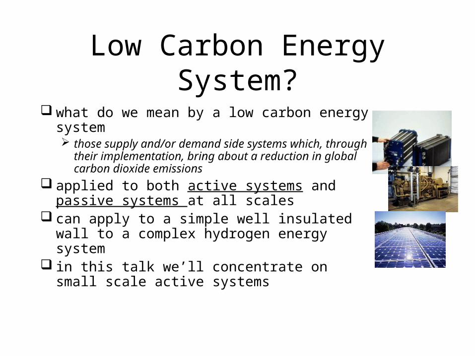
Low Carbon Energy System?

what do we mean by a low carbon energy system those supply and/or demand side systems which,

through their implementation, bring about a reduction in global carbon dioxide emissions

applied to both active systems and passive systems at all scales

can apply to a simple well insulated wall to a complex hydrogen energy system

in this talk we’ll concentrate on small scale active systems

Why Modelling?

appropriate modelling yields information on the operational characteristics and impacts of LCES

supplements and expands upon results from field trials and experimentation

modelling can be used to provide the data needed to back up decisions: from policy to detailed design design: hopefully lead to better performance and/or reduced

energy consumption/emissions strategic: or provide technical evidence for better policy

formulation

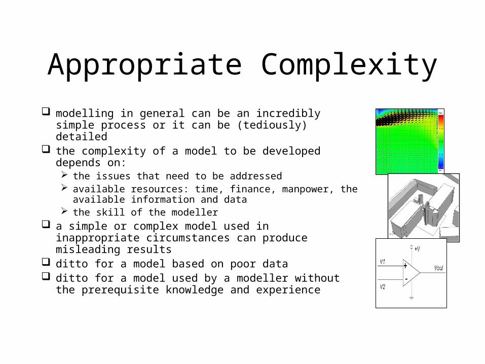
Appropriate Complexity

modelling in general can be an incredibly simple process or it can be (tediously) detailed

the complexity of a model to be developed depends on: the issues that need to be addressed available resources: time, finance, manpower, the

available information and data the skill of the modeller

a simple or complex model used in inappropriate circumstances can produce misleading results

ditto for a model based on poor data ditto for a model used by a modeller without the

prerequisite knowledge and experience

Simple Modelling Example: DHPS

use of a simple model to address a strategic issuewill new DHPS bring about tangible carbon savings?

modelling elements: simple model of electricity supply make-updemand profiles hot water, space heating and for

water for characteristic buildingssimple spreadsheet models of DCHP components

and control

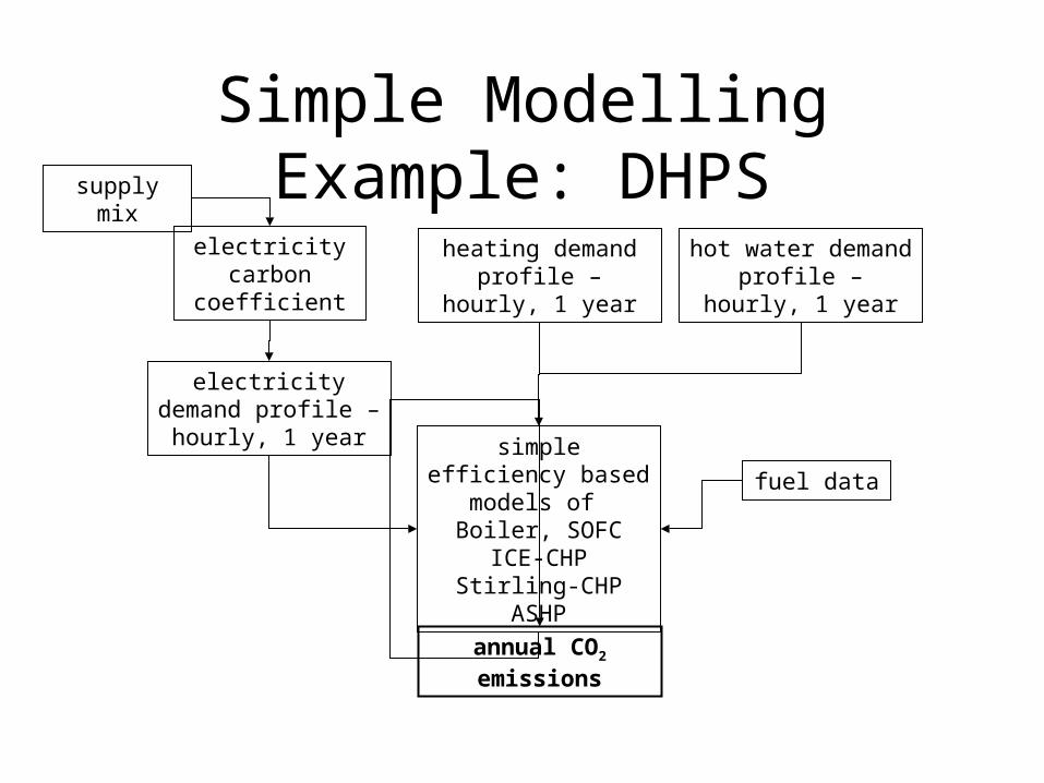
Simple Modelling Example: DHPSsupply mix

electricity carbon

coefficient

heating demand profile – hourly, 1

year

fuel data

hot water demand profile – hourly, 1

year

electricity demand profile – hourly, 1

year simple efficiency based models of Boiler, SOFC ICE-CHP Stirling-CHP

ASHP

annual CO2 emissions

Limitations

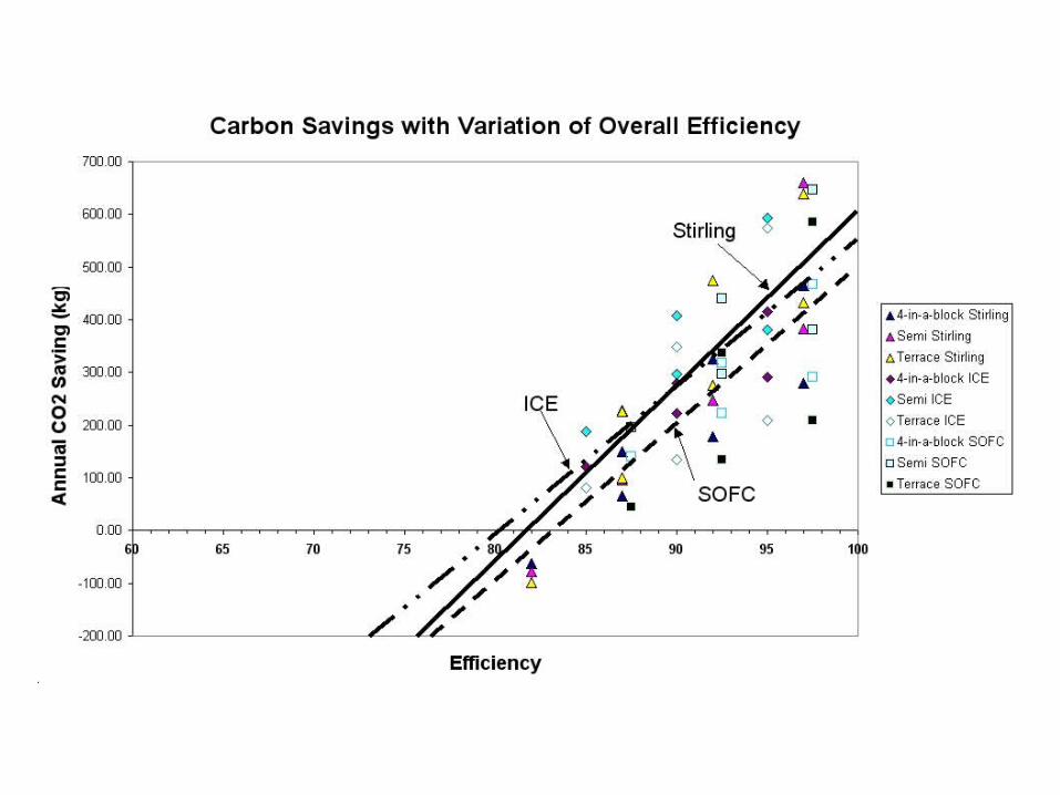
assumed operational efficiencies limited interaction between supply and demand no thermal/electrical storage ideal controller SOFC standby losses not accounted for time averaged heat, hot water and electrical profiles constant carbon coefficient for electricity etc, etc need to take all of this into account when analysing results …

however info is useful in making broad strategic decisions – e.g. deciding in which technologies to invest R&D time

Domain Specific Simulation Environment Example - CFD

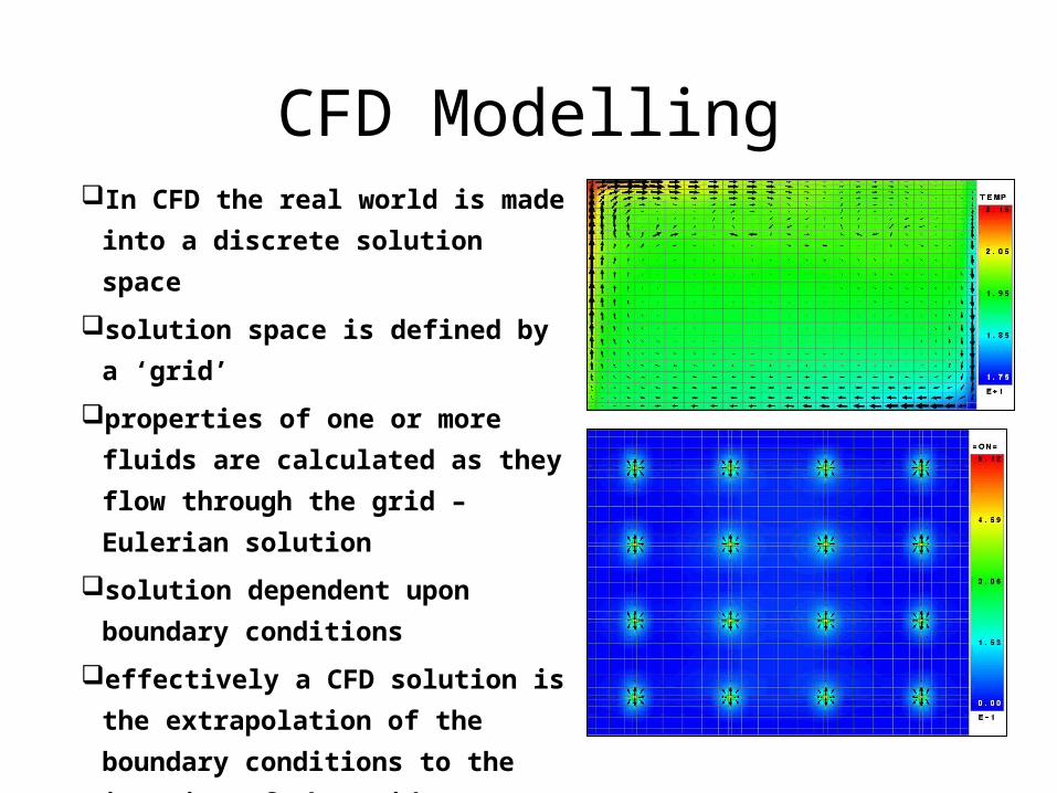
CFD ModellingIn CFD the real world is made into a

discrete solution space

solution space is defined by a ‘grid’

properties of one or more fluids are

calculated as they flow through the

grid – Eulerian solution

solution dependent upon boundary

conditions

effectively a CFD solution is the

extrapolation of the boundary

conditions to the interior of the grid

generally imposing steady state

solution on transient phenomena!

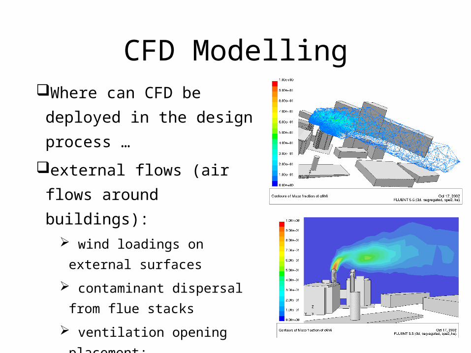
CFD ModellingWhere can CFD be deployed

in the design process …

external flows (air flows

around buildings):

wind loadings on external

surfaces

contaminant dispersal from flue

stacks

ventilation opening placement;

pedestrian comfort

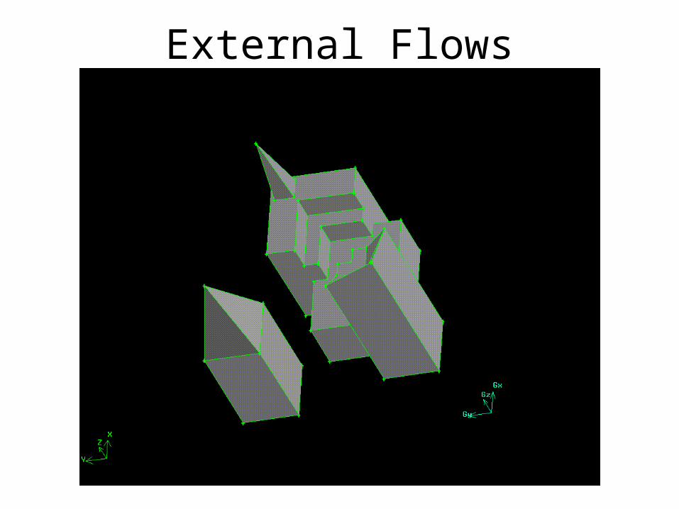
External Flows

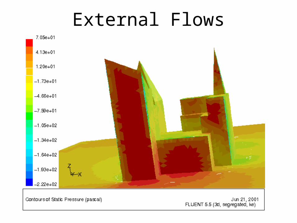
External Flows

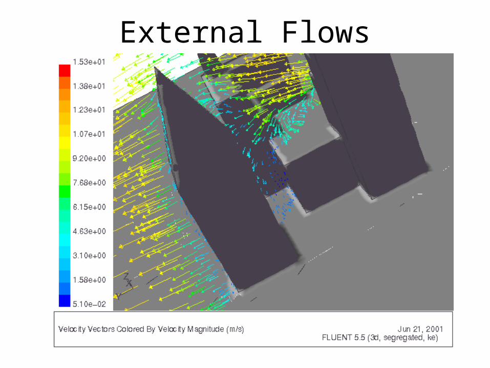
External Flows

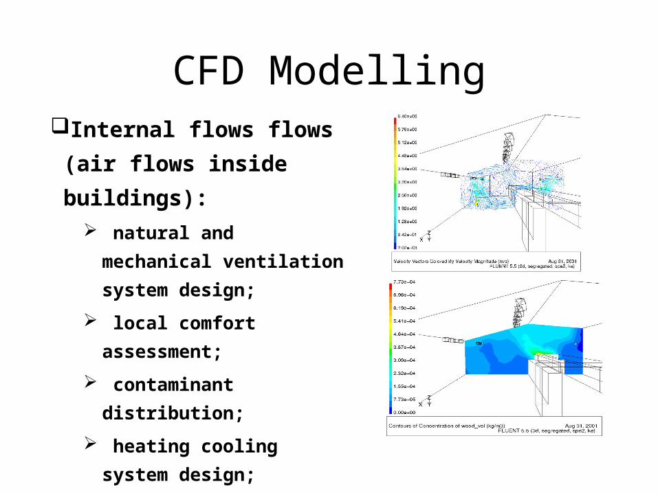
CFD ModellingInternal flows flows (air

flows inside buildings):

natural and mechanical

ventilation system design;

local comfort assessment;

contaminant distribution;

heating cooling system

design;

component design*.

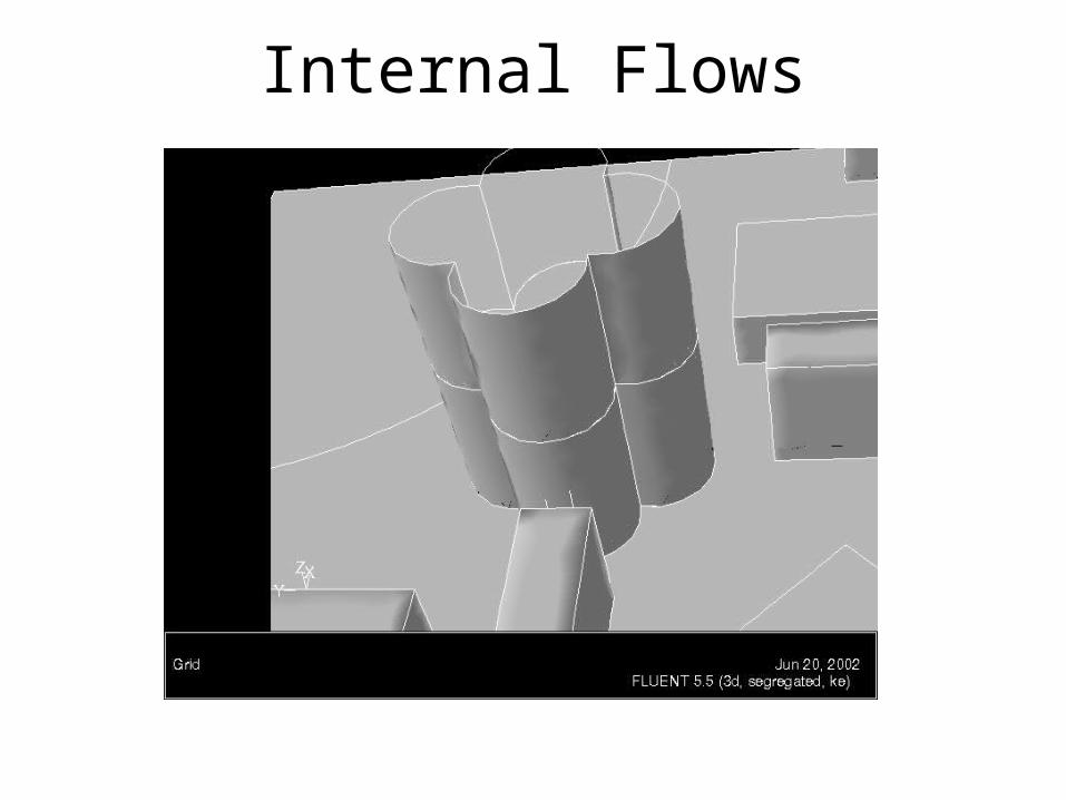
Internal Flows

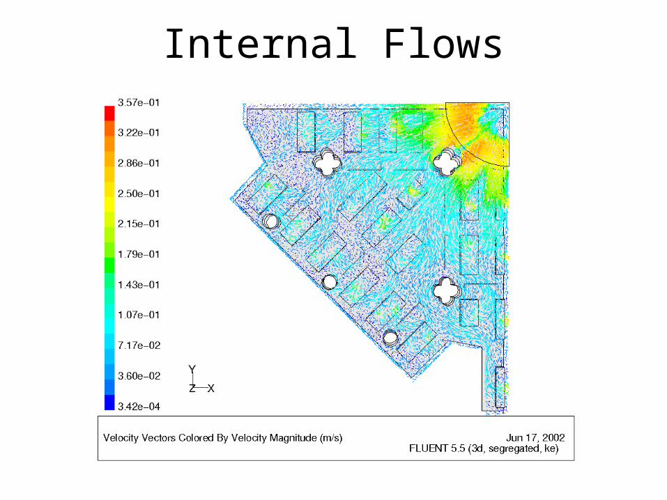
Internal Flows

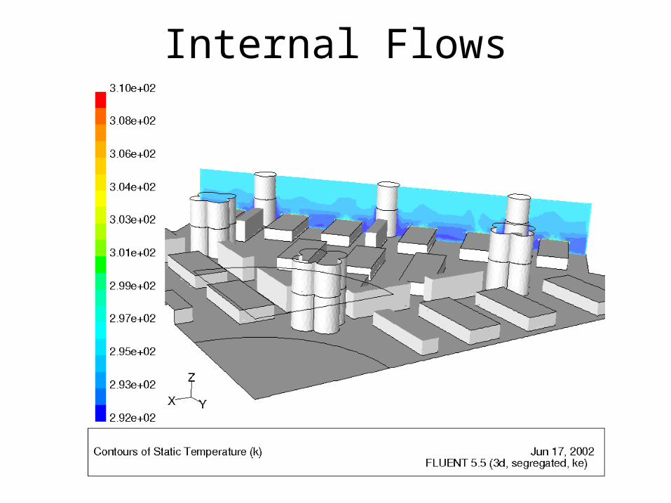
Internal Flows

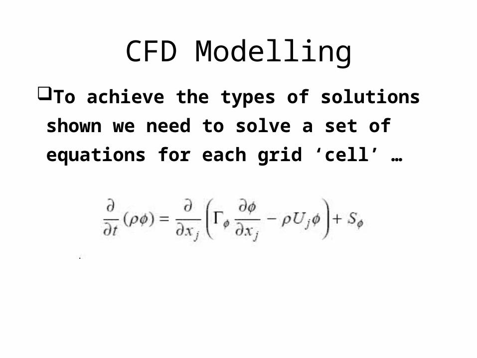
CFD ModellingTo achieve the types of solutions shown

we need to solve a set of equations for

each grid ‘cell’ …

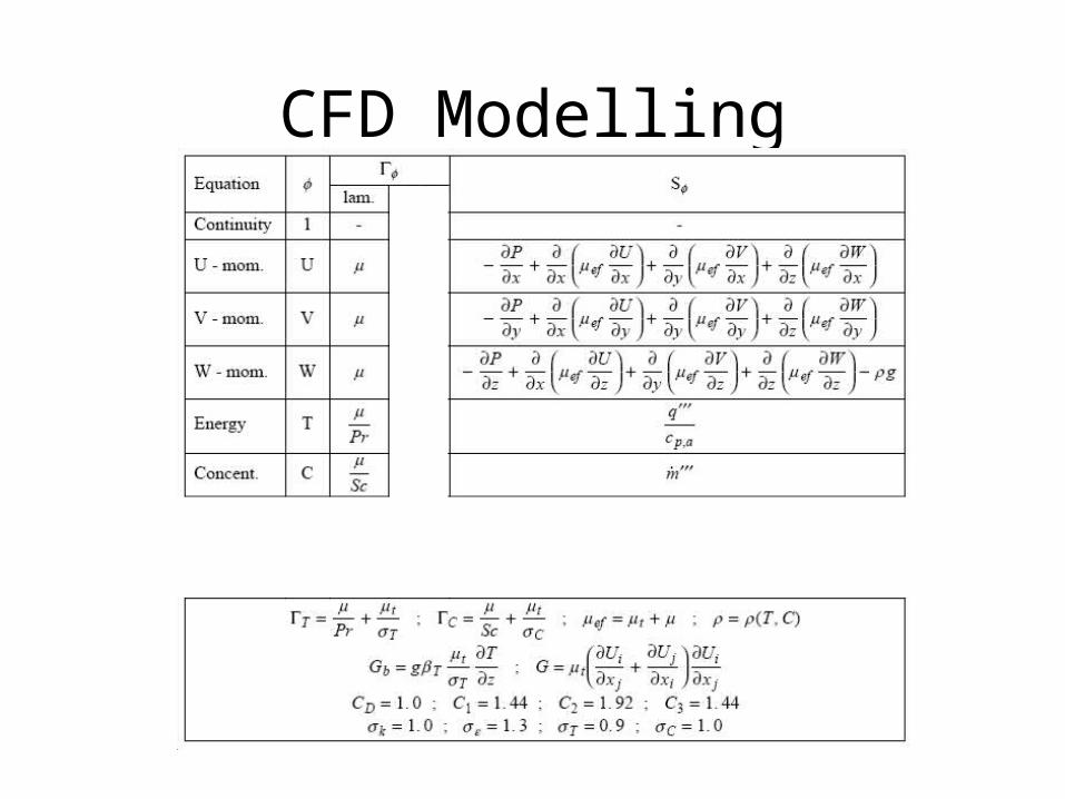
CFD Modelling

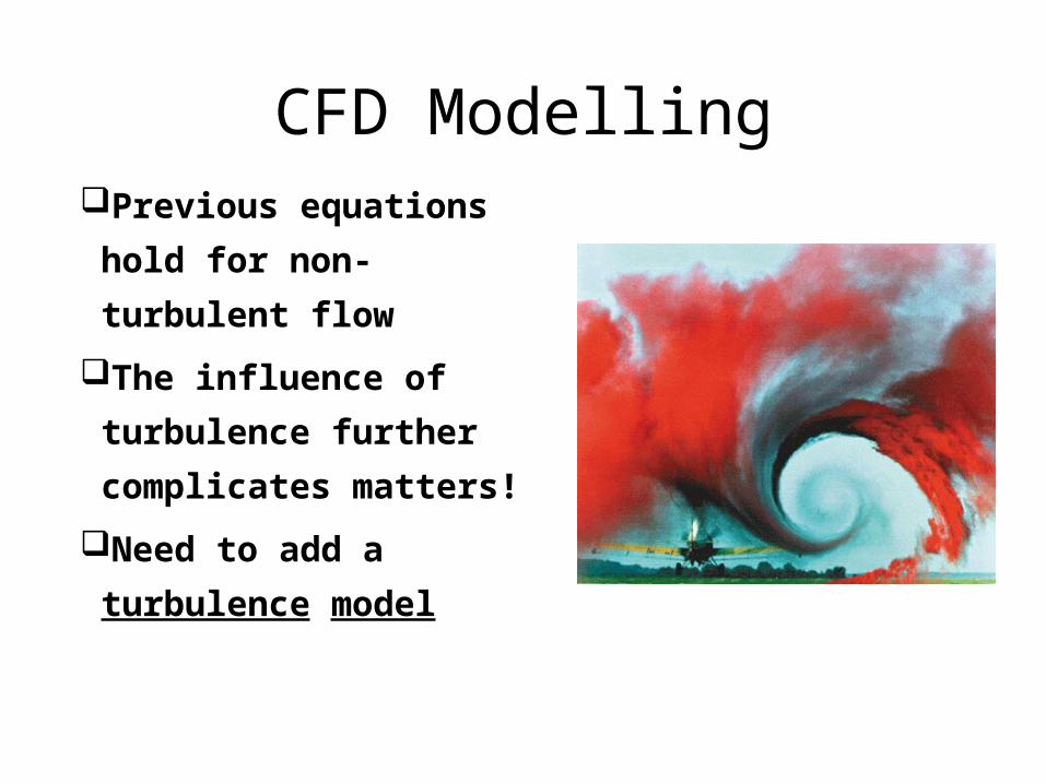
CFD ModellingPrevious equations hold

for non-turbulent flow

The influence of

turbulence further

complicates matters!

Need to add a turbulence

model

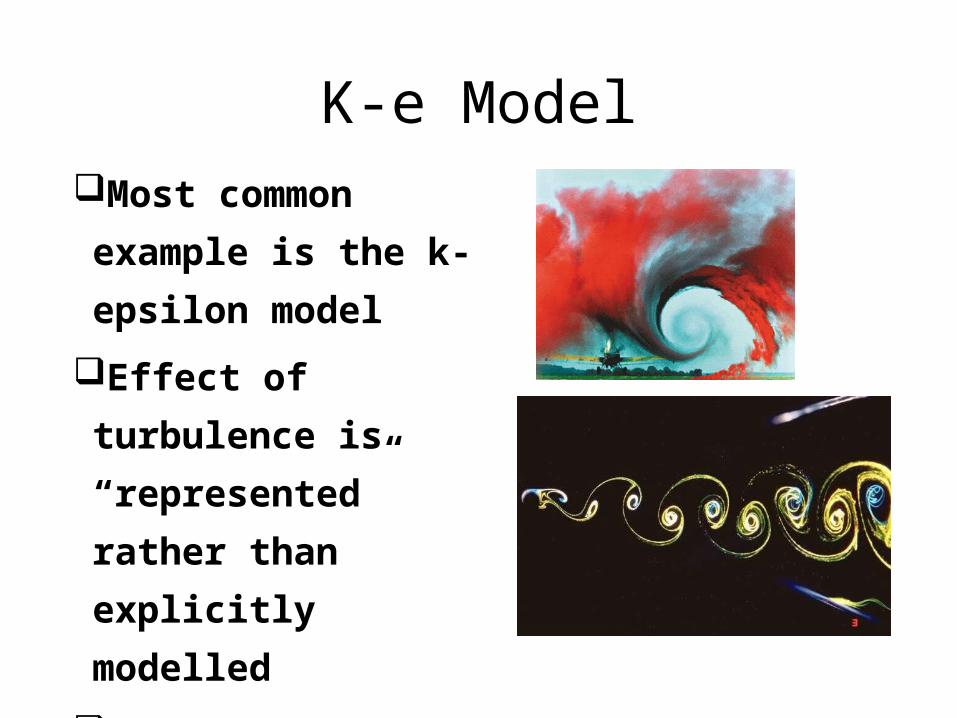
K-e ModelMost common

example is the k-

epsilon model

Effect of turbulence is

“represented” rather

than explicitly

modelled

Two extra equations

need to be solved …

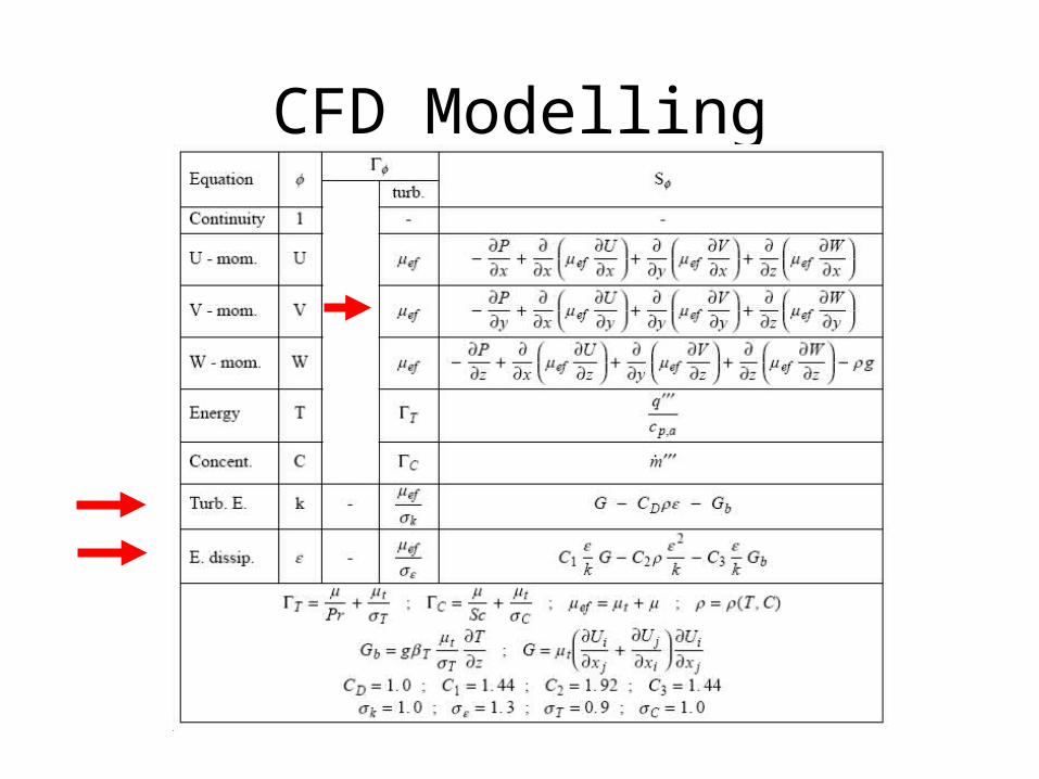
CFD Modelling

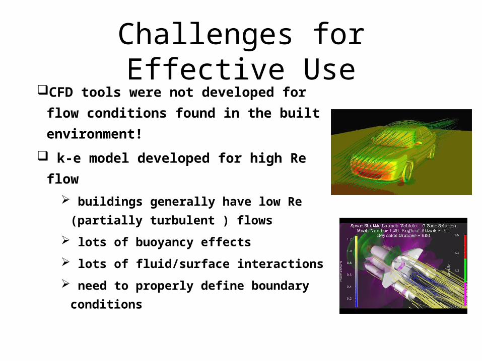
Challenges for Effective UseCFD tools were not developed for flow

conditions found in the built environment!

k-e model developed for high Re flow

buildings generally have low Re (partially

turbulent ) flows

lots of buoyancy effects

lots of fluid/surface interactions

need to properly define boundary conditions

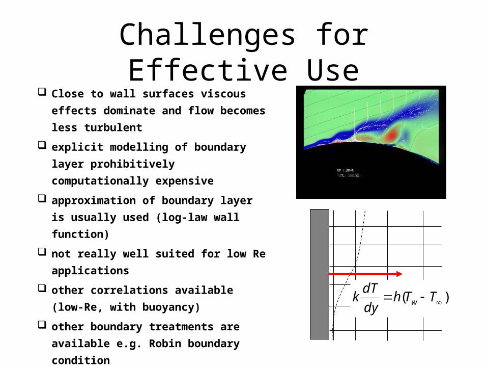
Challenges for Effective Use Close to wall surfaces viscous effects

dominate and flow becomes less turbulent

explicit modelling of boundary layer

prohibitively computationally expensive

approximation of boundary layer is

usually used (log-law wall function)

not really well suited for low Re

applications

other correlations available (low-Re, with

buoyancy)

other boundary treatments are available

e.g. Robin boundary condition )( TThdy

dTk w

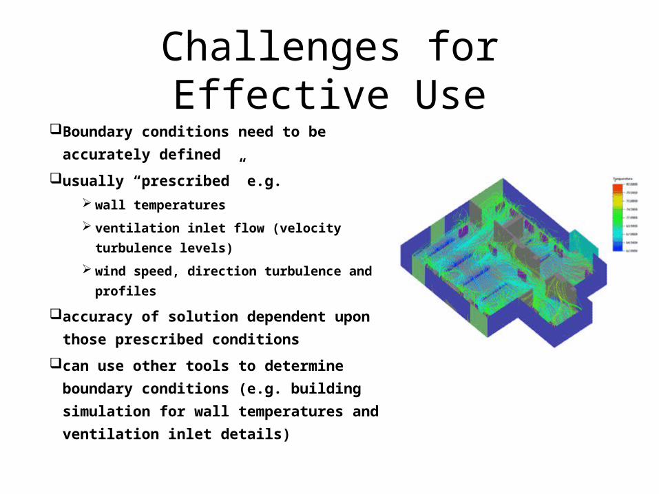
Challenges for Effective UseBoundary conditions need to be accurately

defined

usually “prescribed” e.g.

wall temperatures

ventilation inlet flow (velocity turbulence levels)

wind speed, direction turbulence and profiles

accuracy of solution dependent upon those

prescribed conditions

can use other tools to determine boundary

conditions (e.g. building simulation for wall

temperatures and ventilation inlet details)

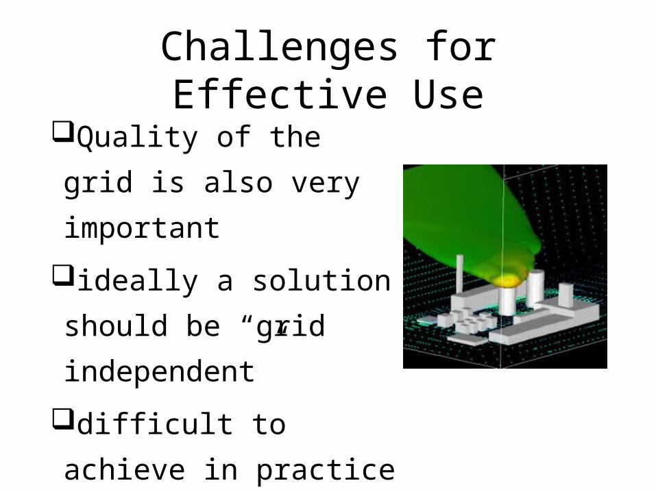
Challenges for Effective Use

Quality of the grid is also

very important

ideally a solution should

be “grid independent”

difficult to achieve in

practice due to time

constraints!

Detailed Modelling previous example described impact of LCES without

modelling operational performance of the LCES system in detail: complexity was hidden behind an average operational efficiency

detailed modelling is appropriate when specific issues associated with the LCES performance are being addressed: impact of thermal storage power quality impact of different control strategies different systems configurations

output from detailed models can feed simpler models (i.e. derive seasonal efficiency for components)

Modelling Tools

there are many options for detailed modelling and can be applied to many ‘domains’ domain specific physical simulation [1]

- FLUENT, PHOENICS, WAMIT …. ‘customised’ simulation environment [2]

- ESP-r, TRNSYS … general purpose modelling environments [3]

- MATLAB (SIMULINK), EES, FEMLAB, SPREADSHEET

try and get over the basic elements behind 2&3 when applied to systems simulation

Customised Simulation Environment Example – Low

Carbon Energy Systems Modelling

Components

components are the fundamental building blocks of all detailed energy modelling applications

basically a component is a self contained mathematical model of a physical process: energy conversion transport of working fluid pressurization heating or cooling phase change control device data recording etc, etc.

can either be used individually or connected together in a systems model (often called a network)

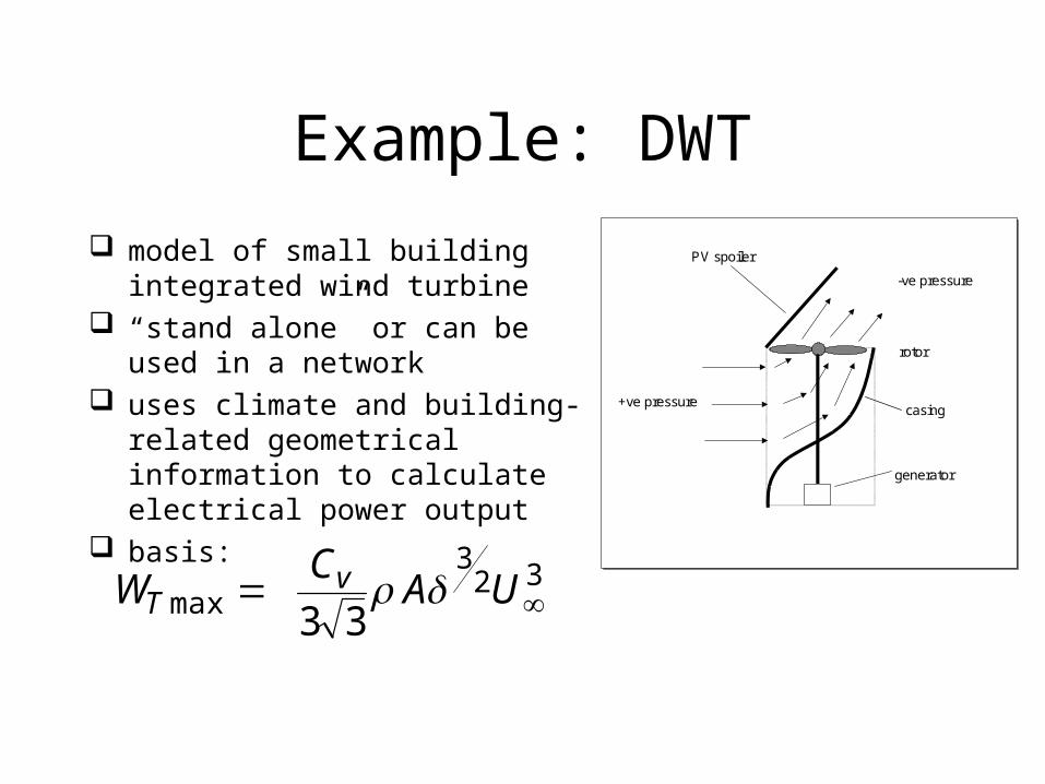
Example: DWT

model of small building integrated wind turbine

“stand alone” or can be used in a network

uses climate and building-related geometrical information to calculate electrical power output

basis:

+ve pressure

-ve pressure

PV spoiler

rotor

generator

casing+ve pressure

-ve pressure

PV spoiler

rotor

generator

casing

323

max 33 UAC

W vT

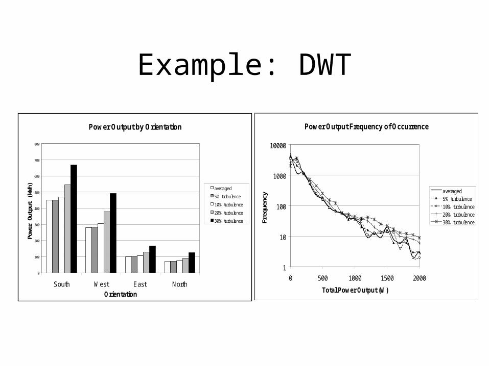
Example: DWT

Power Output by Orientation

0

100

200

300

400

500

600

700

800

South West East NorthOrientation

Pow

er O

utpu

t (kW

h) averaged

5% turbulence

10% turbulence

20% turbulence

30% turbulence

Power Output Frequency of Occurrence

1

10

100

1000

10000

0 500 1000 1500 2000

Total Power Output (W)

Freq

uenc

y

averaged5% turbulence10% turbulence20% turbulence30% turbulence

LCES Components

a word of warning …. LCES is a (relatively) new field the emergence of publicly available robust components lags

behind the evolution of the technology real lack of models for some newer technologies:

fuel cells, ICE CHP, Stirling Engine CHP (IEA annex42) demand side controllers

reasonable coverage of models: PV, Solar thermal, battery storage, power conditioning demand side reduction/management (e.g. lighting control)

Systems Models

systems are modelled by linking together a group of component models – network

LCES model mixture of ‘sexy’ low carbon component models (e.g. hydrogen electrolyser) and mundane BOP – pumps, fans, pipes, etc.

results in a set of consistent or mixed equations describing the LCES

lots of solution options sequential simultaneous mixed (pragmatic!)

objective of solution: determine system performance in user defined sets of circumstances

Systems Models

systems sometimes describe a particular physical ‘domain’ (ESP-r): electrical system fluid flow

specific domain models can be linked together to form an integrated model (ESP-r)

sometimes one system model can be used to describe a multi-domain system (TRNSYS) HVAC integrated hydrogen system

above philosophies require different solution approaches

Sequential Solution

solution is achieved by sequentially solving each component model

output of one model is input to the next good for systems featuring very different model types

– ability to mix and match different models problems with feedback of variables (requires

iteration), solution control, stability can model systems with mixed inputs/outputs

thermal/electrical/control signals

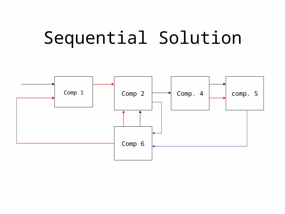
Sequential Solution

Comp 1 Comp 2

Comp 6

Comp. 4 comp. 5

Simultaneous Solution

similar modelling approach for each component simultaneous (matrix) solution of system of equations stable solution mechanism no problems in dealing

with feedback of variables less flexibility in describing and modelling specific

components – models need to be specifically developed for simultaneous solution

systems model usually describes one type of system (e.g. flow, electrical) but possible to combine systems models – integrated systems model

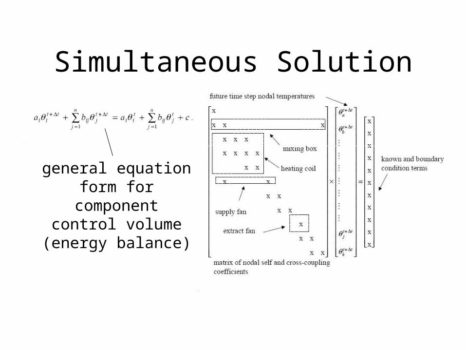
Simultaneous Solution

general equation form for component control

volume (energy balance)

Systems Modelling

ESP-r customised simulation environment lots of ‘domains’ employing same basic modelling approach – finite

volume flux balance systems (fluid flows, plant, electrical), building fabric, moisture all physical elements of model can be described using FVs simultaneous solution of individual domains

boundary conditions for solution from: control criteria climate occupant interaction demand schedules

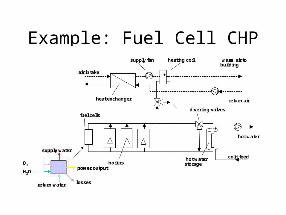
Example: Fuel Cell CHP

+

heating coilsupply fan

heat exchanger

diverting valves

hot waterstorageboilers

fuel cells

warm air tobuilding

hot water

cold feed

return air

air intake +

heating coilsupply fan

heat exchanger

diverting valves

hot waterstorageboilers

fuel cells

warm air tobuilding

hot water

cold feed

return air

air intake

power output

losses return water

supply water

O2

H2O power output

losses return water

supply water

O2

H2O

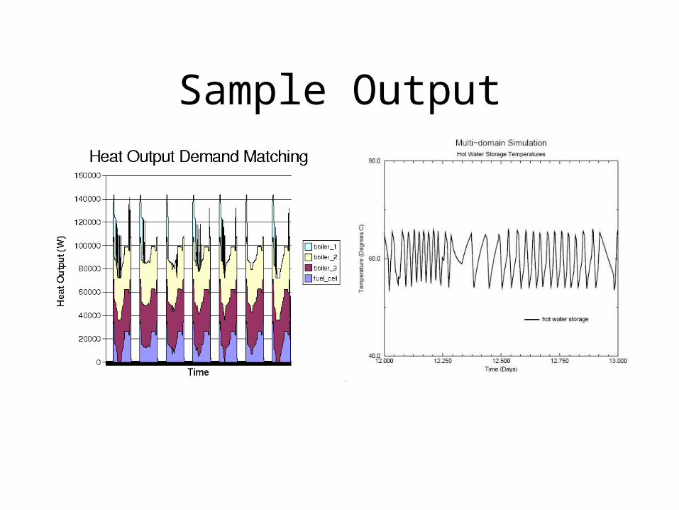
Sample Output

Further Additions

what about the impact on building environment?we can couple systems model to building model

what about adding some other heat power sources?can change model and add more components e.g.

PV what about electrical power output?

we can add more detail (e.g. electrical systems model)

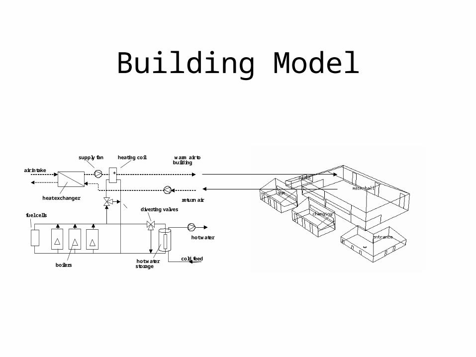
Building Model

+

heating coilsupply fan

heat exchanger

diverting valves

hot waterstorageboilers

fuel cells

warm air tobuilding

hot water

cold feed

return air

air intake +

heating coilsupply fan

heat exchanger

diverting valves

hot waterstorageboilers

fuel cells

warm air tobuilding

hot water

cold feed

return air

air intake

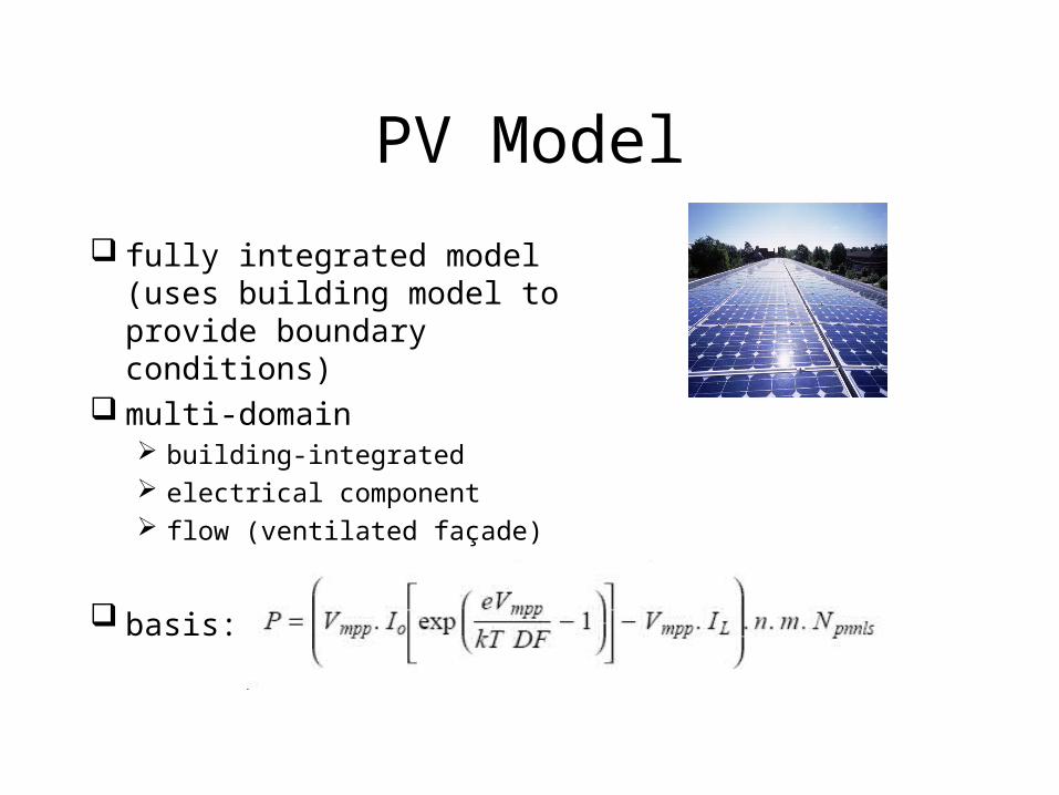
PV Model

fully integrated model (uses building model to provide boundary conditions)

multi-domain building-integrated electrical component flow (ventilated façade)

basis:

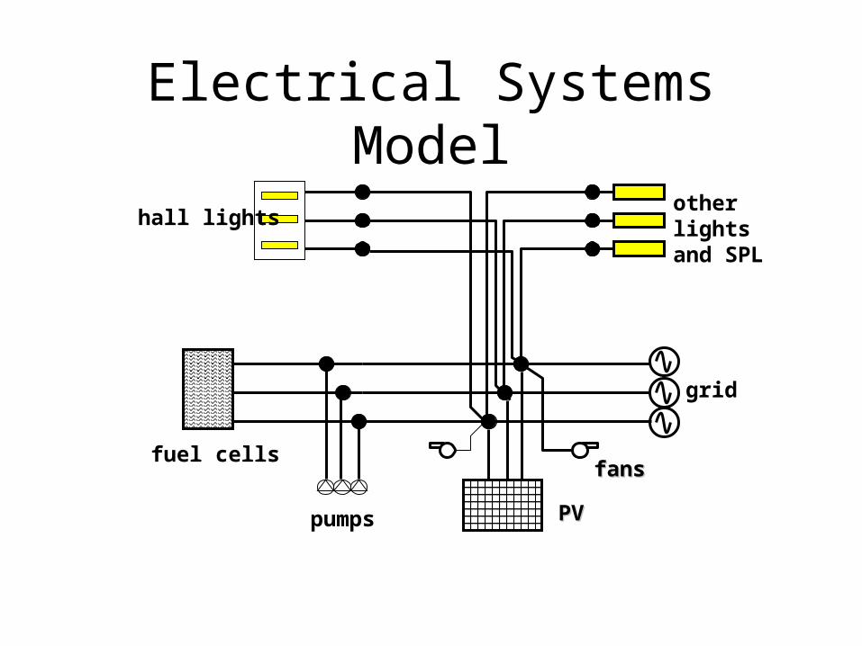
Electrical Systems Model

hall lights

fuel cells

pumps

other lights and SPL

grid

fansfans

PVPV

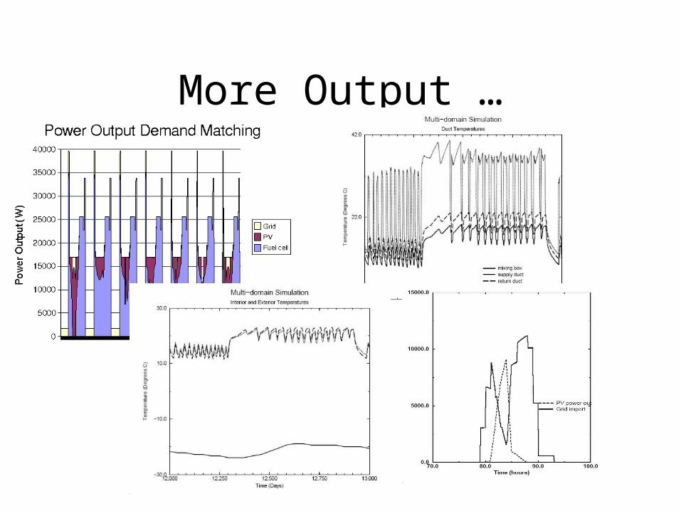
More Output …

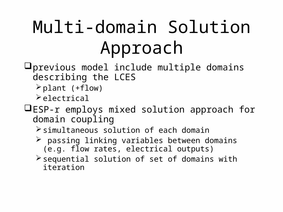
Multi-domain Solution Approach

previous model include multiple domains describing the LCESplant (+flow)electrical

ESP-r employs mixed solution approach for domain coupling simultaneous solution of each domain passing linking variables between domains (e.g. flow

rates, electrical outputs)sequential solution of set of domains with iteration

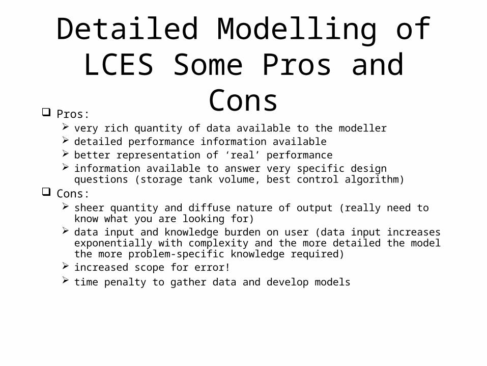
Detailed Modelling of LCES Some Pros and Cons

Pros: very rich quantity of data available to the modeller detailed performance information available better representation of ‘real’ performance information available to answer very specific design questions (storage

tank volume, best control algorithm) Cons:

sheer quantity and diffuse nature of output (really need to know what you are looking for)

data input and knowledge burden on user (data input increases exponentially with complexity and the more detailed the model the more problem-specific knowledge required)

increased scope for error! time penalty to gather data and develop models

Summary important to select appropriate modelling level for the task in hand – diving into

a detailed model is not always a good idea! detailed modelling useful for answering very specific design questions often the

ONLY way to answer these questions used correctly can improve system performance; reduce energy consumption; used incorrectly … lots of detailed modelling tools and approaches available not necessarily geared up to modelling of LCES!! need to weigh advantage of improved results resolution from detailed model

against increased burden of data and knowledge on user! FINALLY important to recognise limitations of model in interpretation of results

….