CE

RN

-TH

ES

IS-2

011-1

80

10

/1

2/

20

11

UNIVERSITY OF HELSINKI REPORT SERIES IN PHYSICS

HU-P-D188

Modelling vacuum arcs:from plasma initiation to surface interactions

Helga Timkó

Division of Materials PhysicsDepartment of Physics

Faculty of ScienceUniversity of Helsinki

Helsinki, Finland

ACADEMIC DISSERTATION

To be presented, with the permission of the Faculty of Science of the University of Helsinki,

for public criticism in the Auditorium XV of the University Main building (Fabianinkatu 33),

on 10th December 2011, at 10 o’clock.

HELSINKI 2011

ISBN 978-952-10-7074-7 (printed version)

ISSN 0356-0961

Helsinki 2011

Helsinki University Printing House (Yliopistopaino)

ISBN 978-952-10-7075-4 (PDF version)

http://ethesis.helsinki.fi/

Helsinki 2011

Electronic Publications @ University of Helsinki (Helsingin yliopiston verkkojulkaisut)

i

Helga Timkó Modelling vacuum arcs: from plasma initiation to surface interactions,

University of Helsinki, 2011, 60 p.+appendices, University of Helsinki Report Series in Physics, HU­P­

D188, ISSN 0356­0961, ISBN 978­952­10­7074­7 (printed version), ISBN 978­952­10­7075­4 (PDF version)

Classification (INSPEC): A5280M, A5280V, A5240H, A5265, A6185, A2915D

Keywords (INSPEC): arcs and sparks, discharges in vacuum, solid­plasma interactions, plasma simula­

tion, molecular dynamics simulation, linear accelerators

Abstract

A better understanding of vacuum arcs is desirable in many of today’s ‘big science’ projects in-

cluding linear colliders, fusion devices, and satellite systems. For the Compact Linear Collider

(CLIC) design, radio-frequency (RF) breakdowns occurring in accelerating cavities influence effi-

ciency optimisation and cost reduction issues. Studying vacuum arcs both theoretically as well as

experimentally under well-defined and reproducible direct-current (DC) conditions is the first step

towards exploring RF breakdowns.

In this thesis, we have studied Cu DC vacuum arcs with a combination of experiments, a

particle-in-cell (PIC) model of the arc plasma, and molecular dynamics (MD) simulations of the

subsequent surface damaging mechanism. We have also developed the 2D ARC-PIC code and the

physics model incorporated in it, especially for the purpose of modelling the plasma initiation in

vacuum arcs.

Assuming the presence of a field emitter at the cathode initially, we have identified the con-

ditions for plasma formation and have studied the transitions from field emission stage to a fully

developed arc. The ‘footing’ of the plasma is the cathode spot that supplies the arc continuously

with particles; the high-density core of the plasma is located above this cathode spot. Our results

have shown that once an arc plasma is initiated, and as long as energy is available, the arc is self-

maintaining due to the plasma sheath that ensures enhanced field emission and sputtering.

The plasma model can already give an estimate on how the time-to-breakdown changes with the

neutral evaporation rate, which is yet to be determined by atomistic simulations. Due to the non-

linearity of the problem, we have also performed a code-to-code comparison. The reproducibility

of plasma behaviour and time-to-breakdown with independent codes increased confidence in the

results presented here.

Our MD simulations identified high-flux, high-energy ion bombardment as a possible mecha-

nism forming the early-stage surface damage in vacuum arcs. In this mechanism, sputtering occurs

mostly in clusters, as a consequence of overlapping heat spikes. Different-sized experimental and

simulated craters were found to be self-similar with a crater depth-to-width ratio of about 0.23 (sim)

– 0.26 (exp).

ii

Experiments, which we carried out to investigate the energy dependence of DC breakdown

properties, point at an intrinsic connection between DC and RF scaling laws and suggest the possi-

bility of accumulative effects influencing the field enhancement factor.

Contents

Abstract i

Contents iii

List of symbols v

1 Introduction 1

2 Purpose and structure of this study 3

2.1 Motivation . . . . . . . . . . . . . . . . . . . . . . . . . . . . . . . . . . . . . . . . . . . . . . . . 3

2.2 Summaries of the original publications . . . . . . . . . . . . . . . . . . . . . . . . . . . . . . 3

2.3 Author’s contribution . . . . . . . . . . . . . . . . . . . . . . . . . . . . . . . . . . . . . . . . . 6

3 Vacuum arcs 7

3.1 Definition and nature of vacuum arcs . . . . . . . . . . . . . . . . . . . . . . . . . . . . . . . 7

3.2 The ‘life cycle’ of vacuum arcs . . . . . . . . . . . . . . . . . . . . . . . . . . . . . . . . . . . . 8

3.3 Observations and facts . . . . . . . . . . . . . . . . . . . . . . . . . . . . . . . . . . . . . . . . 10

3.3.1 Cathode spots and their ‘movement’ . . . . . . . . . . . . . . . . . . . . . . . . . . 11

3.3.2 Field emission . . . . . . . . . . . . . . . . . . . . . . . . . . . . . . . . . . . . . . . . . 12

3.4 Some open questions . . . . . . . . . . . . . . . . . . . . . . . . . . . . . . . . . . . . . . . . . 13

4 Methods 15

4.1 Measurements with the DC setup . . . . . . . . . . . . . . . . . . . . . . . . . . . . . . . . . 15

4.2 Particle-in-cell simulations . . . . . . . . . . . . . . . . . . . . . . . . . . . . . . . . . . . . . . 16

4.2.1 Computer simulation of plasmas . . . . . . . . . . . . . . . . . . . . . . . . . . . . . 17

4.2.2 ARC-PIC simulation procedure and methods . . . . . . . . . . . . . . . . . . . . . 19

4.2.3 Physics model for the vacuum arc . . . . . . . . . . . . . . . . . . . . . . . . . . . . 25

4.3 Molecular dynamics simulations . . . . . . . . . . . . . . . . . . . . . . . . . . . . . . . . . . 27

4.3.1 Solving the equations of motion . . . . . . . . . . . . . . . . . . . . . . . . . . . . . 27

4.3.2 High energy effects: choice of time step and potential . . . . . . . . . . . . . . . 28

4.3.3 Temperature control and boundary conditions . . . . . . . . . . . . . . . . . . . . 29

5 From vacuum arc initiation to extinction 31

5.1 Vacuum arc initiation . . . . . . . . . . . . . . . . . . . . . . . . . . . . . . . . . . . . . . . . . 31

iii

iv CONTENTS

5.2 Early plasma development . . . . . . . . . . . . . . . . . . . . . . . . . . . . . . . . . . . . . . 32

5.2.1 From field emission to a developed vacuum arc . . . . . . . . . . . . . . . . . . . 34

5.2.2 A self-maintaining plasma . . . . . . . . . . . . . . . . . . . . . . . . . . . . . . . . . 35

5.2.3 Plasma expansion and cathode spots . . . . . . . . . . . . . . . . . . . . . . . . . . . 37

5.3 Dependencies and characteristics . . . . . . . . . . . . . . . . . . . . . . . . . . . . . . . . . . 38

5.3.1 What influences the time-to-breakdown . . . . . . . . . . . . . . . . . . . . . . . . 38

5.3.2 Current-voltage characteristic, burning voltage, and energy balance . . . . . . 39

5.4 Early surface damage . . . . . . . . . . . . . . . . . . . . . . . . . . . . . . . . . . . . . . . . . . 41

5.5 Extinction . . . . . . . . . . . . . . . . . . . . . . . . . . . . . . . . . . . . . . . . . . . . . . . . 44

5.6 DC and RF scaling laws . . . . . . . . . . . . . . . . . . . . . . . . . . . . . . . . . . . . . . . . 46

5.7 The field enhancement factor . . . . . . . . . . . . . . . . . . . . . . . . . . . . . . . . . . . . 47

6 Conclusions and outlook 49

Acknowledgements 51

Bibliography 53

v

List of constants and variables

Unless stated otherwise, SI-units are used in this thesis.

Constant Value Quantity

e 1.602176487× 10−19 C elementary chargeħh 1.054571628× 10−34 J s reduced Planck constant

ǫ0 8.854187817× 10−12 F/m permittivity of free space

Variable Quantity

ap acceleration of particle pB magnetic fieldE electric fieldEb breakdown fieldEloc local fieldEsat saturated fieldf distribution functionFp force acting on particle pjmelt threshold of field emission current density that melts the emitterjFN electron field emission current densitymp mass of particle pnp number density of species pp pressurer radial distance in the cylindrical coordinate systemrCu/e neutral evaporation to electron field emission ratioRem emission radius of the field emitterRinj injection radius of field emission electrons and evaporated neutralsrp coordinate of particle pT temperature (in units of energy)vp velocity of particle pvrel relative velocity of two particlesz height coordinate in the cylindrical coordinate system

β field enhancement factorβf field enhancement factor of the flat surfaceΓ ionisation rate∆t time step∆z,∆r grid size

Variable Quantity

ϑ azimuth in the cylindrical coordinate systemλDb Debye lengthln(λ) Coulomb logarithmσ collision cross-sectionφ work functionϕ electric potentialωpe plasma frequency

1 Introduction

Vacuum discharges may appear in different forms in almost every area of today’s big science projects

— may it be unipolar arcs in fusion devices [1–5], multipactor discharges in satellite systems [6–8],

or vacuum arcs in future accelerator designs [9, 10]. Often these discharges are undesired; how-

ever, they may also be used in industry in a controlled manner like in electrical discharge machin-

ing [11, 12], arc welding [13, 14], cutting [15], or in ignition devices [16, 17]. Gaseous arcs and

electrical discharges such as lightnings have been known since ancient times and the processes on-

going in a discharge lamp, for instance, are relatively well understood by now [18, 19]. In contrast,

surprisingly little is understood about the underlying mechanisms of the formation and evolution

of vacuum arcs [20, 21] that can ‘mystically’ form even in ultra high vacuum (UHV) conditions,

where practically no medium between the electrodes is present.

The Compact Linear Collider (CLIC) Study aims at developing a realistic technology for a fu-

ture normal-conducting electron-positron linear collider in the multi-TeV centre of mass energy

range [22]. At the limit of the conventional accelerating technique, the ‘compactness’ of the ma-

chine calls for a high accelerating gradient of 100 MV/m [23], while its efficiency relies on a low

breakdown probability of a few 10−7 1/pulse/m [24], since every vacuum arc in the machine causes

a bunch loss. The constraint on breakdown probability is governed by (i) accelerating length, (ii)

pulse repetition rate, and (iii) the efficiency to be achieved at the interaction point. Reducing the

breakdown probability, however, is desirable not only from the luminosity point of view. Given

the high estimated power consumption of the proposed design (415 MW [25]), efficiency optimi-

sation through breakdown probability reduction could lead to a significant reduction in operation

costs as well.

The present 12 GHz radio-frequency (RF) CLIC accelerating cavity testing strives for perfor-

mance optimisation in order to lay down a baseline concept for the accelerating cavities. When

testing these cavities, incident, transmitted, and reflected signals are monitored all the time. While

normally the transmitted signal is almost the same as the incident signal, on some pulses the trans-

mission drops suddenly to roughly zero and the reflection becomes significant, indicating a break-

down has occurred.

Although RF cavity tests are the most direct way to explore vacuum arcs in CLIC, cavity testing

is time-consuming and costly; thus these tests are not well-suited for studying vacuum arcs. Instead,

vacuum arcs can be generated cost-efficiently and in a controlled manner in two direct-current

(DC) setups at CERN [26, 27]. Despite intrinsic differences between DC and RF testing, the

measurement environment (electric field, pressure in the vacuum chamber, energy available for

1

2

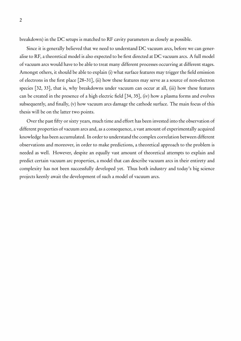
breakdown) in the DC setups is matched to RF cavity parameters as closely as possible.

Since it is generally believed that we need to understand DC vacuum arcs, before we can gener-

alise to RF, a theoretical model is also expected to be first directed at DC vacuum arcs. A full model

of vacuum arcs would have to be able to treat many different processes occurring at different stages.

Amongst others, it should be able to explain (i) what surface features may trigger the field emission

of electrons in the first place [28–31], (ii) how these features may serve as a source of non-electron

species [32, 33], that is, why breakdowns under vacuum can occur at all, (iii) how these features

can be created in the presence of a high electric field [34, 35], (iv) how a plasma forms and evolves

subsequently, and finally, (v) how vacuum arcs damage the cathode surface. The main focus of this

thesis will be on the latter two points.

Over the past fifty or sixty years, much time and effort has been invested into the observation of

different properties of vacuum arcs and, as a consequence, a vast amount of experimentally acquired

knowledge has been accumulated. In order to understand the complex correlation between different

observations and moreover, in order to make predictions, a theoretical approach to the problem is

needed as well. However, despite an equally vast amount of theoretical attempts to explain and

predict certain vacuum arc properties, a model that can describe vacuum arcs in their entirety and

complexity has not been successfully developed yet. Thus both industry and today’s big science

projects keenly await the development of such a model of vacuum arcs.

2 Purpose and structure of this study

2.1 MOTIVATION

The purpose of this study is to better understand the complex plasma-wall interactions that occur

in a vacuum arc. When modelling a transient, non-linear problem, a constant and mutual interplay

between theory and experiments turns out to be an indispensable tool, just as code-to-code com-

parisons are. One of the plasma-wall interactions that has been investigated is the cathode surface

damage caused by the vacuum arc plasma, which provides perhaps the most direct link to experi-

mental observations. A more specific purpose of this study was to obtain a qualitative picture of the

plasma initiation phase after having developed the appropriate tools to this end: a physics model

and a computer code.

The thesis consists of a thesis summary and seven publications, referred to with Roman bold

numbers, six of which have been either published in, accepted in, or submitted to international

peer-reviewed journals and one has been published as a CERN internal technical note.

This thesis is organised as follows: in this Section, a short description of each publication and

the author’s contribution is given. Vacuum arcs are described in Sec. 3. Details on experimental and

numerical methods, as well as on the physics model are given in Sec. 4. All experimental and mod-

elling results are presented in Sec. 5. Conclusions are drawn in Sec. 6. After the acknowledgements

and list of references, the below mentioned publications are attached.

2.2 SUMMARIES OF THE ORIGINAL PUBLICATIONS

In publication I, experimental results of the energy dependence measurements of processing and

breakdown properties, obtained with the DC setup, are detailed. A one- and a two-dimensional

particle-in-cell (PIC) model of plasma initiation in vacuum arcs is presented in publications II and

III, respectively. The software developed for the two-dimensional model is described in IV. A code-

to-code benchmarking study with a simplified discharge model is presented in V. The mechanism

of cathode crater formation due to plasma ions is investigated with the molecular dynamics (MD)

method in VI and is compared to the damage caused by cluster ion bombardment in VII.

PUBLICATION I:

Energy Dependence of Processing and Breakdown Properties of Cu and Mo,

H. Timko, M. Aicheler, P. Alknes, S. Calatroni, A. Oltedal, A. Toerklep, M. Taborelli, W. Wuen-

sch, F. Djurabekova, and K. Nordlund, Physical Review Special Topics – Accelerators and Beams 14,

101003 (2011).

3

4

Experimental results on the energy dependence of Cu and Mo properties measured under DC

conditions are presented in this publication. Besides studying the dependence of the field enhance-

ment factor, saturated field, local field, and damaged area of Cu and Mo on the energy available for

breakdown, a relation between processing efficiency and energy is established as well. For Mo, a

possible explanation of the DC processing mechanism is concluded. The measurements also imply

that certain scaling laws derived from RF cavity testing are valid in DC as well.

PUBLICATION II:

A One-Dimensional Particle-in-Cell Model of Plasma Build-Up in Vacuum Arcs,

H. Timko, K. Matyash, R. Schneider, F. Djurabekova, K. Nordlund, A. Hansen, A. Descoeudres,

J. Kovermann, A. Grudiev, W. Wuensch, S. Calatroni, and M. Taborelli, Contributions to Plasma

Physics 51, 5–21 (2011).

The publication presents a newly developed physics model embedded in a one-dimensional PIC

code, which describes plasma initiation based on the assumption that a field-enhancing feature is

initially present on the cathode. The model includes field emission and neutral evaporation as

initiator mechanisms, and takes several surface processes and collisions into account. Extensive

simulations show how different factors in the model affect, amongst other things, both the time-

to-breakdown and properties of the field emitter. Furthermore, they also identify the prerequisites

for a breakdown to occur.

PUBLICATION III:

Modeling of cathode plasma initiation in copper vacuum arc discharges via particle-in-cell

simulations,

H. Timko, K. Matyash, R. Schneider, F. Djurabekova, K. Nordlund, S. Calatroni, and W. Wuensch,

Physics of Plasmas, submitted for publication (2011).

The previous model has been refined and adapted to a two-dimensional PIC model. This study

focuses on the temporal and spatial evolution of vacuum arcs in their plasma initiation phase and

their interpretation with respect to experimental findings. It identifies the different transitions

leading from field emission to a self-maintaining arc and demonstrates how an arc spot can spread

and potentially initiate other spots at the cathode. With a realistic modelling of the boundary

conditions of the potential, the current-voltage characteristic of arcs is qualitatively investigated,

and thus the model addresses how a steady-state, low-burning-voltage arc is established.

PUBLICATION IV:

2D Arc-PIC Code Description: Methods and Documentation,

5

H. Timko, Technical Report, CERN, CLIC Note 872, (2011).

The two-dimensional PIC code developed specifically for the purpose of the above and future

studies is described in detail in this technical note. In the first part, the different methods used

in the code for the field solver, particle pusher, charge assignment and field interpolation schemes,

collisions, etc. are described. Particular features related to the modelling of vacuum arcs are specified

as well. The second part contains a comprehensive list of equations used in the code, including their

derivation and re-scaling (for efficiency, all equations in the code are dimensionless).

PUBLICATION V:

Why perform code-to-code comparisons: a vacuum arc discharge simulation case study,

H. Timko, P. S. Crozier, M. M. Hopkins, K. Matyash, and R. Schneider, Contributions to Plasma

Physics, accepted for publication (2011).

This publication reports on the outcome of a code-to-code comparison between the 1D ARC-

PIC and the two-dimensional ALEPH codes, carried out with a simplified vacuum arc model. Af-

ter identifying and remedying some software flaws in ALEPH, an excellent agreement in time-to-

breakdown and current density predictions is achieved. Moreover, this benchmarking ‘exercise’

has shown how a given choice of different numerical methods can influence the results when a

non-linear, transient problem is modelled.

PUBLICATION VI:

Mechanism of surface modification in the plasma-surface interaction in electrical arcs,

H. Timko, F. Djurabekova, K. Nordlund, L. Costelle, K. Matyash, R. Schneider, A. Toerklep, G.

Arnau-Izquierdo, A. Descoeudres, S. Calatroni, M. Taborelli, and W. Wuensch, Physical Review B

81, 184109 (2010).

Knowing the properties of plasma ions impinging on the cathode surface, the resulting surface

damage and crater formation was investigated with the MD method. Complex crater shapes as seen

in experiments can form as a result of a heat spike sputtering process, which is due to the high flux

and energy of impinging particles. This heat spike sputtering also leads to an enhanced sputtering

yield in the presence of the plasma. Sputtering takes place mainly in clusters, explaining finger-like

structures observed experimentally. Both simulated and measured crater profiles are shown to be

self-similar over several orders of magnitude, with a characteristic depth-to-width ratio.

PUBLICATION VII:

Crater formation by single ions, cluster ions and ion “showers”,

F. Djurabekova, J. Samela, H. Timko, K. Nordlund, S. Calatroni, M. Taborelli, and W. Wuensch,

6

Nuclear Instruments and Methods in Physics Research B, article in press (2011).

The connection between crater formation mechanisms due to (i) high-flux single ion impact

(ion ‘showers’) and due to (ii) densely packed cluster ions was investigated for 500 eV Au ions. In

both cases, a similar damage can be observed. However, the underlying crater formation mechanism

differs: while ‘showers’ create damage through overlapping heat spikes, cluster ions lead to explosive

cratering that can be identified through an over-densified front on the surface after the impact.

2.3 AUTHOR’S CONTRIBUTION

A substantial part of the experiments presented in publication I was carried out and the rest was

supervised by the author of this thesis, who also suggested and planned the measurements of spot

size development and processing. The data analysis and publication writing was all completed by

the author.

The vacuum arc physics model in II was developed and implemented in the 1D ARC-PIC code

by the author. The author also carried out all simulations and data analysis, and wrote the publica-

tion.

The 2D ARC-PIC code and the refined physics model described in III was developed by the

author, who also performed the simulations and data analysis, and wrote the publication.

The author wrote the entire 2D ARC-PIC code documentation presented in IV and derived the

re-scaled equations therein.

All simulations carried out with the 1D ARC-PIC code in V were performed by the author. The

author also did all the data analysis, and wrote most of the text of the publication, apart from the

ALEPH code description and part of the introduction.

After some initial simulations by co-authors, all systematic simulations and data analysis in VI

was carried out by the author, who also took part in the measurements and wrote most of the

Methods section.

In VII, the author performed the Cu simulations mentioned in the text and provided consulta-

tion on performing and interpreting the Au simulations.

3 Vacuum arcs

Many facts, and thus, much knowledge has been accumulated about vacuum arcs in the past decades.

Nevertheless, many questions regarding why exactly we observe certain behaviours remain still

unanswered, or have been answered only phenomenologically. What exactly a vacuum arc is, what

facts are known, and what the open questions are, is discussed with respect to this thesis below.

3.1 DEFINITION AND NATURE OF VACUUM ARCS

A vacuum arc can be defined as an electric discharge occurring between two electrodes in vacuum.

Perhaps a broader meaning is carried by the term cathodic arcs; these are arc discharges supplied by

the cathode material which can occur either in vacuum or in the presence of an ambient gas [36].

Yet another type of arc is the unipolar arc; unipolar arcs are similar to vacuum arcs, only instead

of striking between two solid electrodes they strike between one solid electrode and a plasma [37]

(e.g. in a tokamak).

One may also distinguish between arcs and sparks. Sparks are momentary gas discharges that

extinguish by themselves once the charges are neutralised; arcs are continuous discharges that are

able to sustain themselves as long as energy and particles are available to the plasma. In other words,

a spark consumes only the electrostatic energy that is stored in the system, while arcs are typically

supplied by an external energy source as well. In another sense (which is not discussed here), sparks

can also refer to chemically burning, hot particles flying off from a material, such as wood.

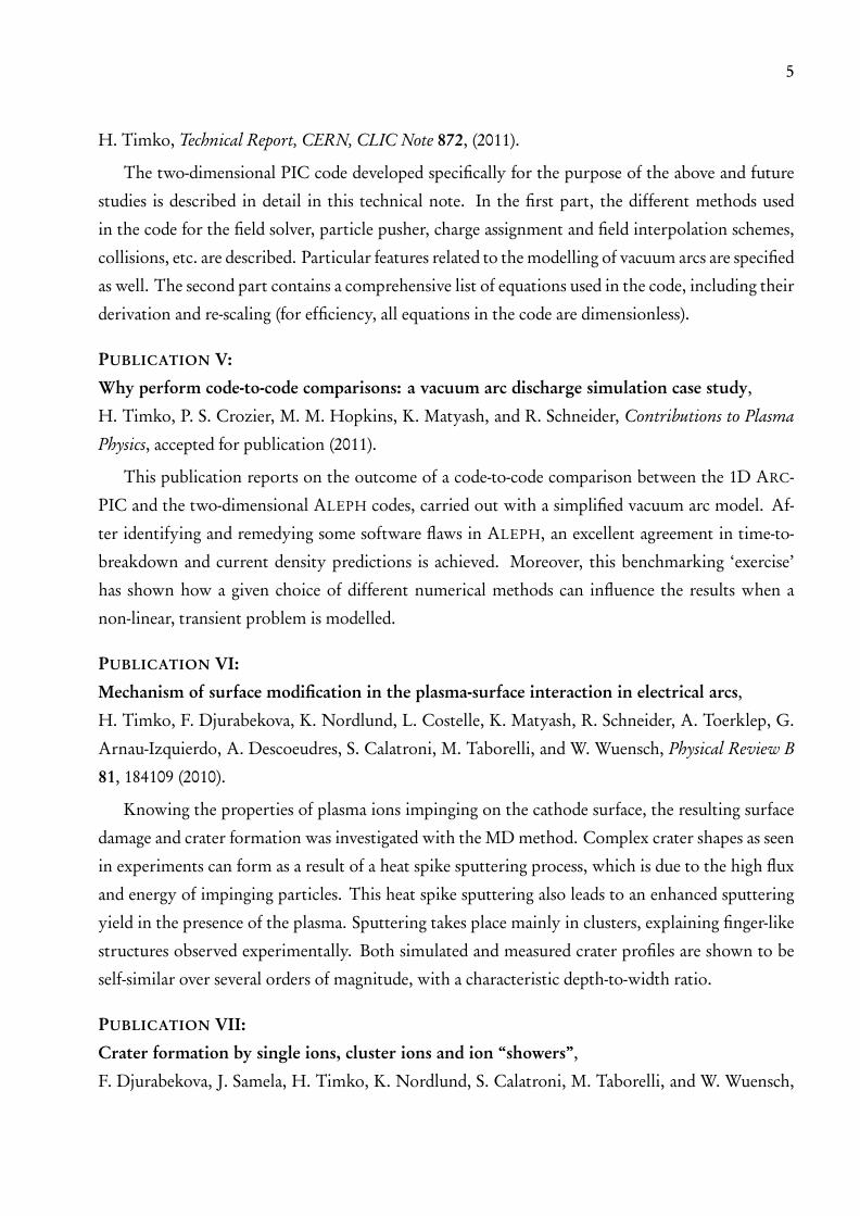
Unless the overall anode temperature is very high, arc discharges are always cathode-

Figure 3.1: Picture of a cathode spottaken 3 µs after ignition with a highspeed camera and an exposure time of50 ns. A figure from [38].

dominated [36]. That is, the plasma particles are supplied

from the cathode material and the anode is only a passive

electron collector. The ‘footings’ of the arc that supply the

plasma and above which the plasma is the densest, are called

cathode spots (Fig. 3.1). In vacuum arcs, the emission of

electrons from the cathode can occur via two mechanisms:

through thermionic emission, when the cathode tempera-

ture is elevated and/or through field emission, in the pres-

ence of high electric fields [31, 39].

In the context of accelerators, the term electrical break-

down is often used and almost always signifies vacuum arc

discharges that affect the accelerator performance. How-

7

8

ever, electrical breakdowns may also occur in solid state dielectrics and in this case may not involve

an arc or plasma at all.

Breakdowns in a CLIC-like environment fall into the category of vacuum arcs that are initiated

due to high electric fields. The dominant electron emission mechanism is field emission. Since the

electrodes are kept at room temperature, the arcs are of the cathodic type. This was also confirmed

by dedicated experiments with the DC setup, which have shown that the breakdown properties

depend only on the cathode material [40]. The measurement techniques of the DC setup shall be

presented in Sec. 4.1.

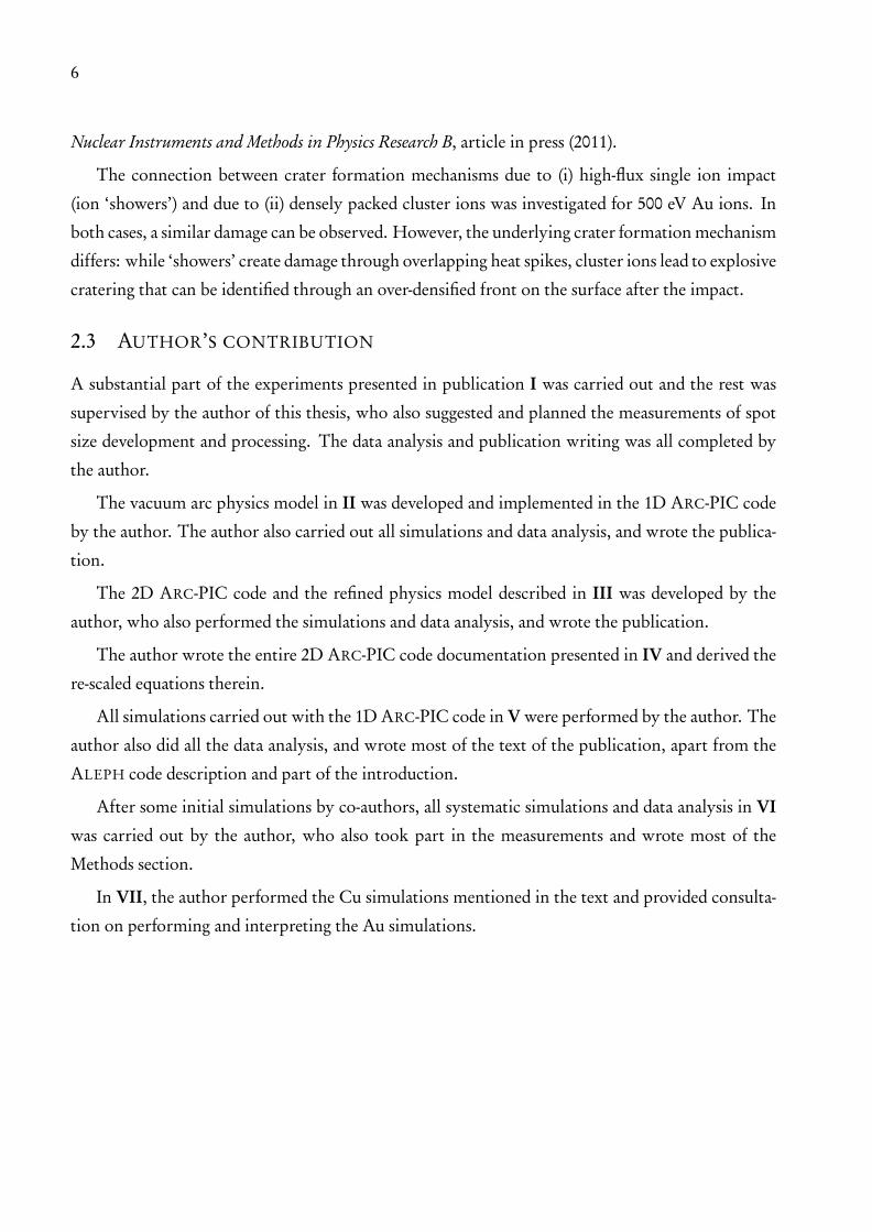
3.2 THE ‘LIFE CYCLE’ OF VACUUM ARCS

Below, we summarise the entire ‘life cycle’ of vacuum arcs that are initiated due to a high electric

field. Our description is based on a phenomenological picture of vacuum arcs [20], which has

become widespread in this field. A schematic illustration of the life cycle is given in Fig. 3.2.

Figure 3.2: Schematic illustration of the life cycle of vacuum arcs initiated due to a high electric fieldin a phenomenological approach. For other types of arcs, the triggering, emission, and evaporationmechanisms may differ. Once the arc reaches stage (4), a continuous burning of the arc is initiated,while the field emitters constantly re-arrange. The life cycle ends and the vacuum arc extinguisheswhen the energy available to the arc is consumed.

9

Some surface features, like impurities or geometrical features (surface roughness, sharp edges)

left over from the manufacturing and machining processes, may be present on the cathode even

prior to applying any electric field. According to some theories, such features may serve as an ini-

tial field emitter that can trigger a breakdown [28]. On the other hand, assuming a well-prepared

surface, the significance of such features can be negligible. Another explanation for the presence of

field emitters on the cathode surface is that they form while a high external electric field is applied

to the surface. From whiskers to voids [32–34], several triggering mechanisms have been proposed.

However, the dominant mechanism, which might depend on the material and its preparation tech-

nique, is still not definite.

Independent of what the triggering mechanism (1) in Fig. 3.2 is, once a strong enough1 emitter

is present, the vacuum arc life cycle can be summarised as follows:

(2) The external electric field is enhanced at the emitter, and field emission of electrons occurs. The

field emission current may heat the emitter significantly [33]. Due to a mixture of high electric

field and temperature effects, the field emitter serves also as a source of non-electron species. As

a consequence, neutrals accumulate above the emitter. At this stage, negative charges dominate

above the emitter and screen the external potential. Thus the field emission current is limited

by the space charge, that is, the spatial charge distribution, of the emitted electrons themselves.

(3) Through ionisation collisions between neutrals and electrons, more and more ions are pro-

duced. After some time, a plasma and with it a plasma sheath are formed. A plasma can be

defined as a gas of particles containing a non-negligible amount of free charges, which is overall

quasi-neutral and governed by a collective behaviour due to the interactions between the free

charges. Whenever a plasma faces an absorbing boundary, a plasma sheath will form at that

boundary, a layer in which the flow velocities of electrons and ions become balanced through a

difference in densities and a corresponding sheath potential that decelerates electrons and accel-

erates ions.

(4) Once a plasma sheath is present, the vacuum arc enters a ‘steady-state’ or self-maintaining

regime that is often referred to as ‘burning’ (which is unrelated to the word’s conventional

meaning of an exothermic chemical reaction). In parallel, the cathode is continuously bom-

barded with ions which leads to crater formation on the surface. How the vacuum arc becomes

self-maintaining, and how craters can be formed during the early stage of arc burning, will be

addressed in Secs. 5.2.2 and 5.4, respectively.

(5) As a consequence of ion bombardment, the cathode surface is strongly modified and the emitter

distribution is re-arranged. At the same time, the electric field can be enhanced locally to high

1The requirements on a field emitter for a vacuum arc to form shall be discussed in Sec. 5.1.

10

values due to the plasma sheath, which can lead to the formation of new field emitters.

A more quantitative picture of what happens during the stages (2)–(5), and what the typical

time- and length scales involved are, shall be given in this thesis. The life cycle of the vacuum arc

comes to an end when the energy available to the arc is exhausted; the vacuum arc extinguishes.

3.3 OBSERVATIONS AND FACTS

The plasma core near the cathode spot can have local electron number densities of up to 1020–

1022 1/cm3 [41, 42], nearing the density of a solid. Further away from the core, the density drops

as the plasma expands into vacuum. Corresponding electron temperatures in the cathode spot are

in the range 1–5 eV [43–45]. For Cu, highly ionised species up to Cu-V can be present [46], with a

mean charge number of two [21].

Vacuum arcs can reach currents up to 10–100 A [21] once they are fully developed. This is

also the typical range seen in experiments with the DC setup (to be discussed in detail in Sec. 5.5).

Current densities in the cathode spot can be as high as 1011–1012 A/m2 [47, 48]. Such extreme

current densities can lead to a fast destruction of sharp tips, that can serve as emitters, in less than a

µs [49, 50].

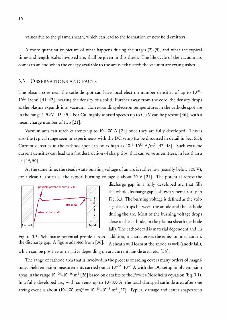
At the same time, the steady-state burning voltage of an arc is rather low (usually below 100 V);

for a clean Cu surface, the typical burning voltage is about 20 V [21]. The potential across the

Figure 3.3: Schematic potential profile acrossthe discharge gap. A figure adapted from [36].

discharge gap in a fully developed arc that fills

the whole discharge gap is shown schematically in

Fig. 3.3. The burning voltage is defined as the volt-

age that drops between the anode and the cathode

during the arc. Most of the burning voltage drops

close to the cathode, in the plasma sheath (cathode

fall). The cathode fall is material dependent and, in

addition, it characterises the emission mechanism.

A sheath will form at the anode as well (anode fall),

which can be positive or negative depending on arc current, anode area, etc. [36].

The range of cathode area that is involved in the process of arcing covers many orders of magni-

tude. Field emission measurements carried out at 10−10–10−9 A with the DC setup imply emission

areas in the range 10−20–10−16 m2 [26] based on data fits to the Fowler-Nordheim equation (Eq. 3.1).

In a fully developed arc, with currents up to 10–100 A, the total damaged cathode area after one

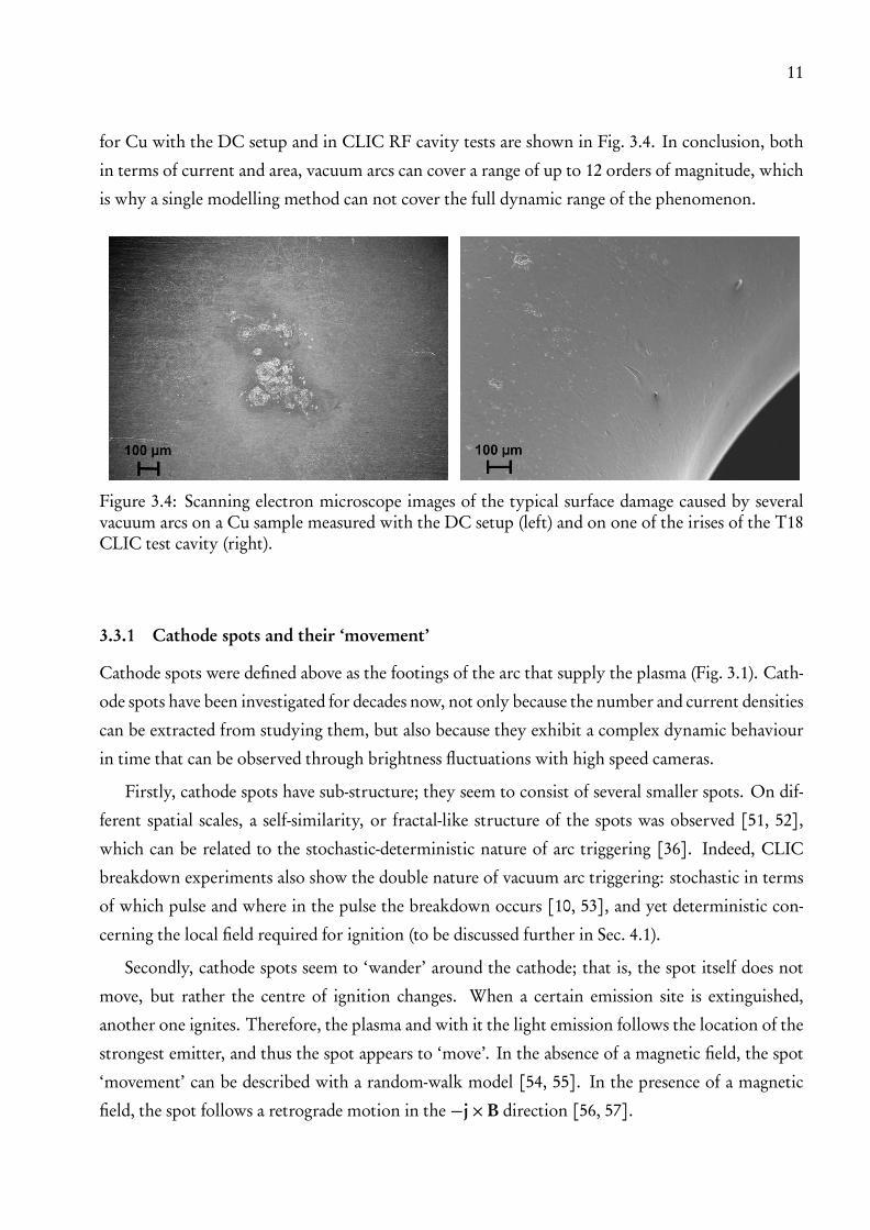
arcing event is about (10–100 µm)2 = 10−10–10−8 m2 [27]. Typical damage and crater shapes seen

11

for Cu with the DC setup and in CLIC RF cavity tests are shown in Fig. 3.4. In conclusion, both

in terms of current and area, vacuum arcs can cover a range of up to 12 orders of magnitude, which

is why a single modelling method can not cover the full dynamic range of the phenomenon.

Figure 3.4: Scanning electron microscope images of the typical surface damage caused by severalvacuum arcs on a Cu sample measured with the DC setup (left) and on one of the irises of the T18CLIC test cavity (right).

3.3.1 Cathode spots and their ‘movement’

Cathode spots were defined above as the footings of the arc that supply the plasma (Fig. 3.1). Cath-

ode spots have been investigated for decades now, not only because the number and current densities

can be extracted from studying them, but also because they exhibit a complex dynamic behaviour

in time that can be observed through brightness fluctuations with high speed cameras.

Firstly, cathode spots have sub-structure; they seem to consist of several smaller spots. On dif-

ferent spatial scales, a self-similarity, or fractal-like structure of the spots was observed [51, 52],

which can be related to the stochastic-deterministic nature of arc triggering [36]. Indeed, CLIC

breakdown experiments also show the double nature of vacuum arc triggering: stochastic in terms

of which pulse and where in the pulse the breakdown occurs [10, 53], and yet deterministic con-

cerning the local field required for ignition (to be discussed further in Sec. 4.1).

Secondly, cathode spots seem to ‘wander’ around the cathode; that is, the spot itself does not

move, but rather the centre of ignition changes. When a certain emission site is extinguished,

another one ignites. Therefore, the plasma and with it the light emission follows the location of the

strongest emitter, and thus the spot appears to ‘move’. In the absence of a magnetic field, the spot

‘movement’ can be described with a random-walk model [54, 55]. In the presence of a magnetic

field, the spot follows a retrograde motion in the −j×B direction [56, 57].

12

3.3.2 Field emission

For vacuum arcs occurring between room temperature electrodes that are exposed to a high exter-

nal electric field E , the dominant electron emission mechanism is field emission. The field emission

current density jFN can be calculated from the electron tunneling probability over a potential bar-

rier that is lowered by the presence of the electric field; this current density is described by the

Fowler-Nordheim formulae. The original form of the Fowler-Nordheim equation was derived for

the tunneling of an electron through a triangular potential barrier [58]. The form used in the ex-

periments and simulations presented in this thesis is based on a more realistic power-law potential

barrier in the Murphy and Good formulation [39, 59–61]:

jFN(Eloc) =IFN(Eloc)

Aem

= aFN

(eEloc)2

φ t (y)2exp

−bFN

φ3/2v(y)

eEloc

!

, (3.1)

where IFN is the field emission current, Aem is the emission area, φ is the work function, e the

elementary charge, and Eloc the local field to be defined shortly. The valueφ= 4.5 eV [62] has been

used as an average both for polycrystalline Cu and Mo (investigated in publication I). t (y) and v(y)

are elliptical integral functions of the variable

y =

√

√

√

√

e3Eloc

4πǫ0φ2

, (3.2)

where ǫ0 is the permittivity of vacuum. The constants aFN and bFN stand for

aFN =e

16π2ħh= 1.5414× 10−6

A

eV,

bFN =4p

2me

3ħh= 6.8309× 109

1p

eVm, (3.3)

when [ jFN] = A/m2, [Eloc] = V/m and [φ] = eV, and where ħh is the reduced Planck constant

and me the electron mass. The Wang and Loew approximation [63] has been used for the elliptic

functions t (y) and v(y), setting t (y) = 1 and v(y) = 0.956− 1.062y2.

Unless measuring field emission very close to the surface (e.g. in field electron microscopy), the

variable appearing in Eq. 3.1 is not simply E as one would expect, but is replaced with Eloc

def.= βE ,

containing the field enhancement factor β. This field enhancement factor is a phenomenological

factor that was originally introduced as a constant, because currents obtained in field emission

measurements from large areas — even though following the Fowler-Nordheim trend — turned out

to be much higher than what would be expected based on purely E [61, 64].

13

The field enhancement factor is usually attributed to ‘protrusions’ on the cathode surface that

can locally enhance the external electric field. One way to enhance the field is through the presence

of geometrical features (emitter ‘tips’) that curve and densify the field lines at sharp edges. The

geometrical field enhancement of a spherically rounded tip, for instance, is frequently approximated

as β = h/r + 2 [65], where h is the height and r the radius of the tip. Hence, to explain the

experimentally observed β ® 100 for Cu, a 10 nm broad tip would have to be about 500 nm high.

Nobody has ever observed such features; nevertheless, their existence cannot be excluded since they

might simply not be present when the electric field is off and the surfaces are observed.

An alternative explanation of highβ values is given by Schottky’s conjecture on the multiplica-

tion of field enhancement factors, sometimes also called ‘tip on tip’ model. In this model, the final

β is interpreted as a compound of a larger tip with βl — stemming from surface roughness, for in-

stance — and a smaller tip with βs placed on top of it, resulting in a multiplicative enhancement of

β≈βlβs [66]. Another way of obtaining an enhanced electron current could be a locally lowered

work function (cf. Eq. 3.1), when impurities or crystallographic defects are present on or close to

the surface.

3.4 SOME OPEN QUESTIONS

It remains to be proven by future experiments which features serve as a source of enhanced field

emission and how a β can be assigned to these features. What triggers an arc is also investigated in

ongoing theoretical studies [34]; however, knowing the origin of β is not essential for the studies

presented here. Nevertheless, it should be pointed out thatβ is not necessarily a constant but could

depend on other quantities such as E .

All this relates to another question, namely to whether and to what extent breakdown initia-

tion is stochastic or deterministic in its nature. RF Cu cavity tests, for instance, have shown a flat

breakdown distribution over the RF pulse length [53], suggesting a purely probabilistic occurrence.

In contrast, DC Cu breakdown rate experiments interleaved with field emission scans (cf. Sec. 4.1)

have shown that β grows from pulse to pulse prior to breakdown and the breakdown determinis-

tically occurs when a given Eloc is exceeded [67]. Future experiments are planned to investigate the

stochastic/deterministic nature of breakdowns further.

Furthermore,β evolving from pulse-to-pulse indicates that the repetitive application of E could

alter the surface and thus there could be a ‘memory effect’. If so, β could depend on several quan-

tities such as E , the pulse length, the energy stored in the pulse, etc. The possible dependence of

β on other quantities is only one of the open questions to which experiments shall give an answer.

Another essential question is how RF and DC breakdowns relate to each other and how results

14

obtained in one case can be translated to the other.

Once the field emission is already present, what remains to be understood is under what condi-

tions a plasma will form and what the role of the local field in the initiation of the plasma is. Also,

a plasma model should explain how this field emission can turn into a fully developed arc.

• What are the transitions the breakdown undergoes during this time?

• How do we get from nano-scale field emission areas to macroscopic damaged spots?

• Can the cathode spot expand and how can we interpret its ‘movement’?

• How does the discharge gap evolve from a high-voltage open-circuit element to a low-burning-

voltage plasma?

All these questions are going to be addressed in Sec. 5.

The properties of a self-maintaining arc plasma and the role of the plasma sheath in this process

are yet to be determined. Furthermore, the lifetime of an arc and what makes it extinguish also

need to be understood. Modelling a non-linear phenomenon, it is also desirable to investigate what

factors in the numerical model may influence the results and predictions of the model.

Finally, since the interaction between the plasma and the cathode surface is essential for vacuum

arcs, a link between plasma fluxes and sputtering yields should be established and incorporated into

both the plasma and the surface damage model. Moreover, obtaining a better understanding of

the crater formation mechanism of breakdowns could help to compare the experiments with the

theory.

4 Methods

Studying vacuum arcs is a challenging task mainly because the different phenomena occurring at

different stages of a vacuum arc are all interconnected and cannot be treated ignoring this connec-

tion. Therefore many areas of physics are inseparably involved in the modelling, and the choice of

tools must reflect this fact. In the following, experimental as well as plasma and materials science

simulation tools are presented.

4.1 MEASUREMENTS WITH THE DC SETUP

In the DC setup, measurements of DC vacuum arcs are carried out under UHV conditions in the

pressure range 2×10−11–10−9 mbar. Discharges are generated between a rectangular Cu sample (the

cathode) and a spherically rounded Cu rod with a diameter of 2.3 mm (the anode), see Fig. 4.1.

The cathode is grounded at all times and the anode is typically powered with +1–2 kV during

Figure 4.1: Discharge gap in one ofthe DC setups at CERN.

field emission scans and +4–6 kV during breakdown field mea-

surements. With a discharge gap separation of about 20 µm, the

latter translates to an electric field of 200–300 MV/m, which is

also a typical surface field in RF accelerating cavities [22, 68].

With the aid of field emission scans, the field emission cur-

rent IFE as a function of external electric field E can be ob-

tained. Measuring in the range where space charge effects are

negligible, that is 2× 10−11–10−9 A in the present setup (the

lower limit corresponds to limitations in the measurement

technique), the field enhancement factor β can be obtained

by a fit to the Fowler-Nordheim equation (Eq. 3.1).

In breakdown field measurements, the external electric field

is ramped up step-wise in order to determine the highest elec-

tric field that can be sustained without a breakdown occurring.

This field is the breakdown field Eb. Note that during the voltage ramp the current rises explosively,

in a very non-linear manner (cf. Eq. 3.1). Measuring Eb repeatedly on the same spot, some materials

exhibit conditioning (e.g. Cu) and some de-conditioning (e.g. Mo), which means that after a given

amount of breakdown events, Eb is higher or lower, respectively, than on an undamaged surface;

i.e. processing occurs1. The average breakdown field that is reached after processing is called the

1Solely the cathode is processed here, since the anode is processed with breakdowns on a separate spot, beforeacquiring measurement data. After that, measurements are taken on another, virgin spot on the cathode.

15

16

saturated field Esat; this Esat characterises how ‘resistant’ a material is to breakdowns and thus allows

us to rank materials according to this property [40, 69]. Combining field emission scans prior to

breakdown and breakdown field measurements afterwards, the local field Eloc = βEb for Cu, after

processing, was found to always have about the same value, ECuloc∼ 10–11 GV/m [67].

It should be remarked that DC processing differs from RF cavity processing in mainly two

aspects: (i) having different energy flows and electrostatic instead of electromagnetic fields and (ii)

the area probed by the breakdown events: in DC, a small area with a radius of around 800 µm is

probed over and over again, whereas in RF most of the breakdowns occur on undamaged areas.

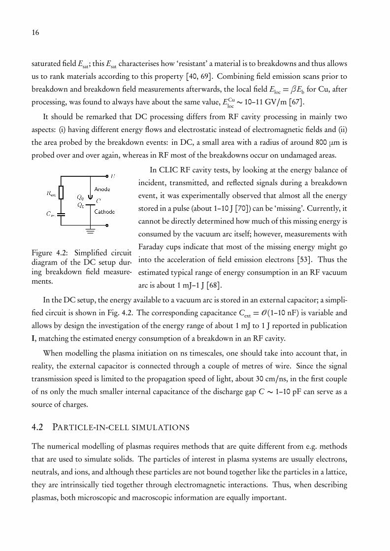
Figure 4.2: Simplified circuitdiagram of the DC setup dur-ing breakdown field measure-ments.

In CLIC RF cavity tests, by looking at the energy balance of

incident, transmitted, and reflected signals during a breakdown

event, it was experimentally observed that almost all the energy

stored in a pulse (about 1–10 J [70]) can be ‘missing’. Currently, it

cannot be directly determined how much of this missing energy is

consumed by the vacuum arc itself; however, measurements with

Faraday cups indicate that most of the missing energy might go

into the acceleration of field emission electrons [53]. Thus the

estimated typical range of energy consumption in an RF vacuum

arc is about 1 mJ–1 J [68].

In the DC setup, the energy available to a vacuum arc is stored in an external capacitor; a simpli-

fied circuit is shown in Fig. 4.2. The corresponding capacitance Cext = O (1–10 nF) is variable and

allows by design the investigation of the energy range of about 1 mJ to 1 J reported in publication

I, matching the estimated energy consumption of a breakdown in an RF cavity.

When modelling the plasma initiation on ns timescales, one should take into account that, in

reality, the external capacitor is connected through a couple of metres of wire. Since the signal

transmission speed is limited to the propagation speed of light, about 30 cm/ns, in the first couple

of ns only the much smaller internal capacitance of the discharge gap C ∼ 1–10 pF can serve as a

source of charges.

4.2 PARTICLE-IN-CELL SIMULATIONS

The numerical modelling of plasmas requires methods that are quite different from e.g. methods

that are used to simulate solids. The particles of interest in plasma systems are usually electrons,

neutrals, and ions, and although these particles are not bound together like the particles in a lattice,

they are intrinsically tied together through electromagnetic interactions. Thus, when describing

plasmas, both microscopic and macroscopic information are equally important.

17

For the plasma simulations presented in publication III, the sequential 2D ARC-PIC code has

been used. Plasma initiation in vacuum arcs has been simulated with total run times of up to ∼ 1–

1.5 months, using up to 1.5 million particles. Amongst others, the 2D ARC-PIC code shall be

described below.

4.2.1 Computer simulation of plasmas

In principle, the dynamics of a plasma can be fully described by the Newton-Maxwell system of

equations. On the other hand, due to the usually large number of particles in a plasma and limited

computational capacity, keeping track of all individual particles is in practice unrealistic; simpli-

fied approaches are necessary. Depending on whether predominantly microscopic or macroscopic

information is required in the given problem and depending on applicability, a kinetic or fluid de-

scription may be used. However, the applicability of these methods is largely dependent on the

collisionality of the plasma in question.

In the fluid description, the plasma is treated as a single macroscopic object, a ‘conductive fluid’,

that obeys besides hydrodynamic equations also Maxwell’s equations. Computational fluid models

aim at determining the evolution of hydrodynamic macroscopic quantities in a system, such as mass

density, current density, and macroscopic (bulk plasma) velocity. Perhaps the simplest approach is

ideal magnetohydrodynamics, which is a single fluid description that treats the fluid as a perfect

conductor.

More sophisticated approaches, such as multi-fluid models describing different species sepa-

rately, exist as well. Generally, fluid approaches are based on assumptions concerning the equation

of state, electrical resistivity, and above all, collisionality. Since fluid models are based on classical

thermodynamics and hydrodynamics, the applicability of a fluid model is restricted to strongly

collisional plasmas that are in quasi-static equilibrium, that is, they follow locally a Maxwell-

Boltzmann distribution.

In plasmas that are far from a Maxwell-Boltzmann distribution and/or in collisionless plasmas

where thermalisation cannot take place, a kinetic description can be used. Kinetic models aim at

describing the spatial and temporal evolution of both microscopic and macroscopic quantities such

as number density n, temperature T , pressure p, and local information on particle positions r and

velocities v and thus can capture the velocity distribution function locally in the plasma. In a kinetic

description, the macroscopic quantities need to be derived from the microscopic quantities.

Kinetic theory has its roots in assuming a weakly coupled plasma where multiple particle cor-

relations of three or more particles can be neglected. Starting from a fundamental level, a plasma

in which the number of particles for each species is conserved will obey the continuity equation of

18

the particle distribution function f = f (t ,r,v) in phase space:

d f

dt=∂ f

∂ t+∂ ( f v)

∂ r+∂ ( f a)

∂ v= 0 . (4.1)

Here t , r, and v are independent variables, so∇r ·v= 0. If now the plasma is perfectly collisionless

such that the particles are uncorrelated, one may assume ∇v · a = 0 as well. Thus the fundamental

equation of the collisionless kinetic theory, the Vlasov equation [71], takes the following form:

∂ f

∂ t+ v ·

∂ f

∂ r+

F

m·∂ f

∂ v= 0 , (4.2)

where in plasma physics applications, F usually stands for the Lorentz force F = q(E+ v× B).

Collisions, however, introduce additional forces to the system and alter the evolution of the distri-

bution f . Thus in collisional kinetic theory, by introducing a collision operator we arrive at the

Boltzmann (sometimes also called the Vlasov-Fokker-Planck) equation [72]:

∂ f

∂ t+ v ·

∂ f

∂ r+

F

m·∂ f

∂ v=

�

∂ f

∂ t

�

c

. (4.3)

Although the Fokker-Planck-Maxwell system has less degrees of freedom (DOF) than the origi-

nal Newton-Maxwell system, fully solving Eq. 4.3 for a tokamak plasma, for instance, is currently

still too demanding [73]. To reduce the complexity of the kinetic problem, gyrokinetic and gy-

rofluid models have been developed [74] for the simulation of magnetised plasmas. Gyrokinetic

models aim at reducing one of the six DOF in Eq. 4.3 by moving to guiding-centre2 coordinates and

ignoring the rapidly changing gyrophase of the particle, while taking into account kinetic effects

such as the effect of a finite Larmor radius [73]. Two main types of gyrokinetic models exist [75]:

(i) the Lagrangian approach that samples the distribution function via marker particles and (ii) the

Vlasov or Eulerian models that use a continuum approach to describe f .

On the boundary between kinetic and fluid description there are, for instance, gyrofluid models

that construct different moments of Eq. 4.3 (or Eq. 4.2) and apply an appropriate closure, assuming

thereby an equilibration of flows and currents [76]. Kinetic and fluid descriptions may also be

coupled in hybrid models [77].

For the modelling of plasma initiation in vacuum arcs, the particle-in-cell method [77–80] has

been applied. PIC is a commonly used method in the area of plasma physics that is based on

2In the presence of a uniform or spatially and/or temporally slowly varying magnetic field, the trajectory of acharged particle can be described as a superposition of a fast gyromotion around the magnetic field lines and a slowdrift of the guiding centre of this gyromotion.

19

a kinetic description using the Lagrangian approach. The kinetic approach is essential for the

modelling of the transient plasma initiation phase, where the velocity distributions are far from

Maxwellian. Moreover, only the self-consistent treatment of particle-induced and external fields of

the PIC method can allow for an appropriate treatment of a system where high electric fields and

boundaries (absorbing walls) are present.

With the PIC method, particles are described in a continuous phase space, in a Lagrangian (mov-

ing) reference frame, while plasma macroscopic quantities (potential, densities, etc.) are discretised

onto mesh points in a Eulerian (stationary) frame. Thus the two main components of a PIC code,

the particle mover and the field solver, operate in different spaces. To obtain the forces acting on

particles that enter the particle mover, a field interpolation method is required that interpolates the

electric field from grid points to particle positions. To obtain the charge density that enters the field

solver, charge assignment to the grid points has to be carried out, which extrapolates the number

density from the particle positions. In order to limit the DOF in the system, the PIC method makes

use of the fact that the acceleration due to the Lorentz force depends only on the charge-to-mass ra-

tio (Eq. 4.5b) by simulating superparticles, which correspond to many real particles but are treated

by the code as a single particle.

4.2.2 ARC-PIC simulation procedure and methods

Plasma initiation in vacuum arcs has been modelled with two sequential, electrostatic PIC codes:

the 1D ARC-PIC code [81] and the 2D ARC-PIC code described in publications III and IV. The

1D ARC-PIC and the 2D ARC-PIC codes use a Cartesian and a cylindrically symmetric coordinate

system, respectively. The discharge gap consists of two parallel electrodes in both cases. In the

cylindrically symmetric system, the two coordinates are the distance from the cathode z and the

distance from the symmetry axis r . Since both codes apply the same computational methods, the

same simulation procedure, and differ mainly in their dimensionality, only the 2D ARC-PIC code

is discussed below; the equations of the 1D ARC-PIC Cartesian code can be obtained in the limit

r = 0.

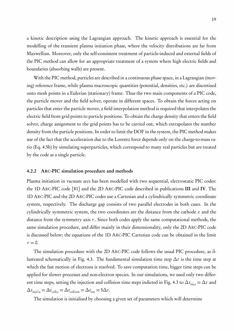
The simulation procedure with the 2D ARC-PIC code follows the usual PIC procedure, as il-

lustrated schematically in Fig. 4.3. The fundamental simulation time step ∆t is the time step at

which the fast motion of electrons is resolved. To save computation time, bigger time steps can be

applied for slower processes and non-electron species. In our simulations, we used only two differ-

ent time steps, setting the injection and collision time steps indicted in Fig. 4.3 to ∆tinj,e =∆t and

∆tinj,Cu =∆tcoll,e =∆tcoll,ion =∆tion = 5∆t .

The simulation is initialised by choosing a given set of parameters which will determine

20

Figure 4.3: Schematic of the simulation procedure in the 2D ARC-PIC code. Some steps in theprocedure are carried out only at a multiple of the fundamental time step.

• the external electric circuit,

• the properties of the field emitter,

• the system size and the numerical resolution: the time step ∆t , the grid size ∆z, and the

real-to-superparticle ratio NSP.

The numerical resolution applied in the simulation has to be suitably ‘guessed’ initially. To

ensure the validity of this ‘guess’ and the stability of the solution, the fulfilment of the following

stability conditions is followed regularly in the code:

∆t ® 0.2ω−1pe

, (4.4a)

∆z ® 0.5λD , (4.4b)

21

where ωpe =

Ç

e2ne

ǫ0 meis the plasma frequency and λD =

Ç

ǫ0Te

e2nethe Debye length. These constraints

can be estimated considering the harmonic oscillations of a linear, unmagnetised plasma [78, 82].

The real-to-superparticle ratio has to be chosen such that the amount of particles is large enough

during the field emission phase to avoid numerical instabilities and, at the same time, low enough

in the final stage of the simulation to avoid memory overflow.

The simulation will start from perfect vacuum, assuming a field emitter that has the chosen

characteristics. This field emitter is a source of electron field emission and Cu neutral evaporation

right from the beginning. Once particles are present in the system, collisions can take place in the

discharge gap and plasma-wall interactions at the boundaries. At the same time, the electric circuit

parameters will determine the total energy available for breakdown, and thus the evolution of the

external potential at the electrodes. The details and assumptions of the physics model incorporated

into the code shall be given in Sec. 4.2.3.

Over the entire simulation time, output is generated typically a few hundred times. The output

contains the phase-space coordinates of the superparticles, the macroscopic quantities of the plasma

derived from these coordinates, as well as information on the particle currents at the boundaries

and resulting electric circuit parameters.

Given that the simulated phenomenon can produce explosively a large amount of particles,

there can be several reasons for the simulation to stop:

• the density grows so high that the stability conditions (Eq. 4.4) are not fulfilled anymore and

the solution becomes unreliable,

• the number of particles grows so high that memory limitations are reached,

• the chosen total simulation time tmax is completed.

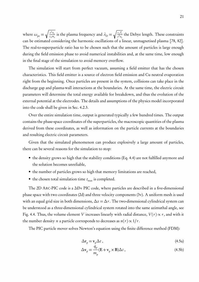
The 2D ARC-PIC code is a 2d3v PIC code, where particles are described in a five-dimensional

phase space with two coordinates (2d) and three velocity components (3v). A uniform mesh is used

with an equal grid size in both dimensions,∆z =∆r . The two-dimensional cylindrical system can

be understood as a three-dimensional cylindrical system rotated into the same azimuthal angle, see

Fig. 4.4. Thus, the volume element V increases linearly with radial distance, V (r )∝ r , and with it

the number density n a particle corresponds to decreases as n(r )∝ 1/r .

The PIC particle mover solves Newton’s equation using the finite difference method (FDM):

∆rp = vp∆t , (4.5a)

∆vp =qp

mp

(E+ vp×B)∆t , (4.5b)

22

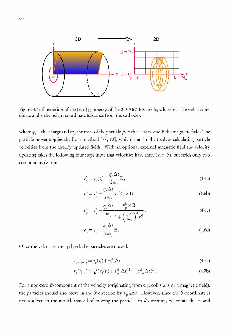
Figure 4.4: Illustration of the (r, z)-geometry of the 2D ARC-PIC code, where r is the radial coor-dinate and z the height coordinate (distance from the cathode).

where qp is the charge and mp the mass of the particle p, E the electric and B the magnetic field. The

particle mover applies the Boris method [77, 83], which is an implicit solver calculating particle

velocities from the already updated fields. With an optional external magnetic field the velocity

updating takes the following four steps (note that velocities have three (z, r,ϑ), but fields only two

components (z, r )):

vap= vp(ti)+

qp∆t

2mp

E , (4.6a)

vbp= va

p+

qp∆t

2mp

vp(ti)×B , (4.6b)

vcp= va

p+

qp∆t

mp

vbp×B

1+�

qp∆t

2mp

�2

B2

, (4.6c)

vdp= vc

p+

qp∆t

2mp

E . (4.6d)

Once the velocities are updated, the particles are moved:

zp(ti+1) = zp(ti)+ vdp,z∆t , (4.7a)

rp(ti+1) =q

(rp(ti)+ vdp,r∆t )2+ (vd

p,ϑ∆t )2 . (4.7b)

For a non-zero ϑ-component of the velocity (originating from e.g. collisions or a magnetic field),

the particles should also move in the ϑ-direction by vp,ϑ∆t . However, since the ϑ-coordinate is

not resolved in the model, instead of moving the particles in ϑ-direction, we rotate the r - and

23

ϑ-components of the particle velocity into a frame where ϑ vanishes again. This rotation is deter-

mined by the angle α= arcsin

�

vdp,ϑ∆t

rp(ti+1)

�

:

�

vp,r(ti+1)

vp,ϑ(ti+1)

�

=

�

cosα sinα− sinα cosα

�

vdp,r

vdp,ϑ

!

. (4.8)

Having thus calculated the new particle positions and velocities, the updated forces and fields

are obtained by solving the 2D cylindrical Poisson equation for the electric potential ϕ:

�

∂ 2

∂ r 2+

1

r

1

∂ r+∂ 2

∂ z2

�

ϕ =e

ǫ0

(ni− ne) , (4.9)

where ni and ne are ion and electron number densities, respectively. A five-point difference approxi-

mation is used to discretise the above expression with the FDM at a given mesh point (z = k , r = j ):

∑

5-p.

cmϕm ≡ cj-1,kϕj-1,k+ cj,k-1ϕj,k-1+ cj,kϕj,k+ cj,k+1ϕj,k+1+ cj+1,kϕj+1,k =e

ǫ0

(nij,k− ne

j,k) , (4.10)

where the constants cm are mesh-point dependent. The above sparse matrix inversion problem is

efficiently solved with the lower-upper factorisation method using the SUPERLU package [84].

The linear cloud-in-cell scheme [77] is used to both interpolate the electric field from grid points

Figure 4.5: The ‘shape’ of a particle (red dot) in thecloud-in-cell scheme and the value of the weight-ing function W = W (r, z) at the grid pointsaround the particle.

to particle positions, and to extrapolate num-

ber densities from particle positions to grid

points, see Fig. 4.5. On a uniform grid,

choosing the same schemes for field interpola-

tion and charge assignment ensures appropri-

ate space-symmetry of forces and momentum

conservation [82].

Developed for the treatment of copper

plasma with three species, e−, Cu, and Cu+, the

ARC-PIC codes include collision routines de-

veloped at the Max-Planck-Institut für Plasma-

physik [85]. Collisions are described with the

Monte Carlo algorithm, which is based on the

24

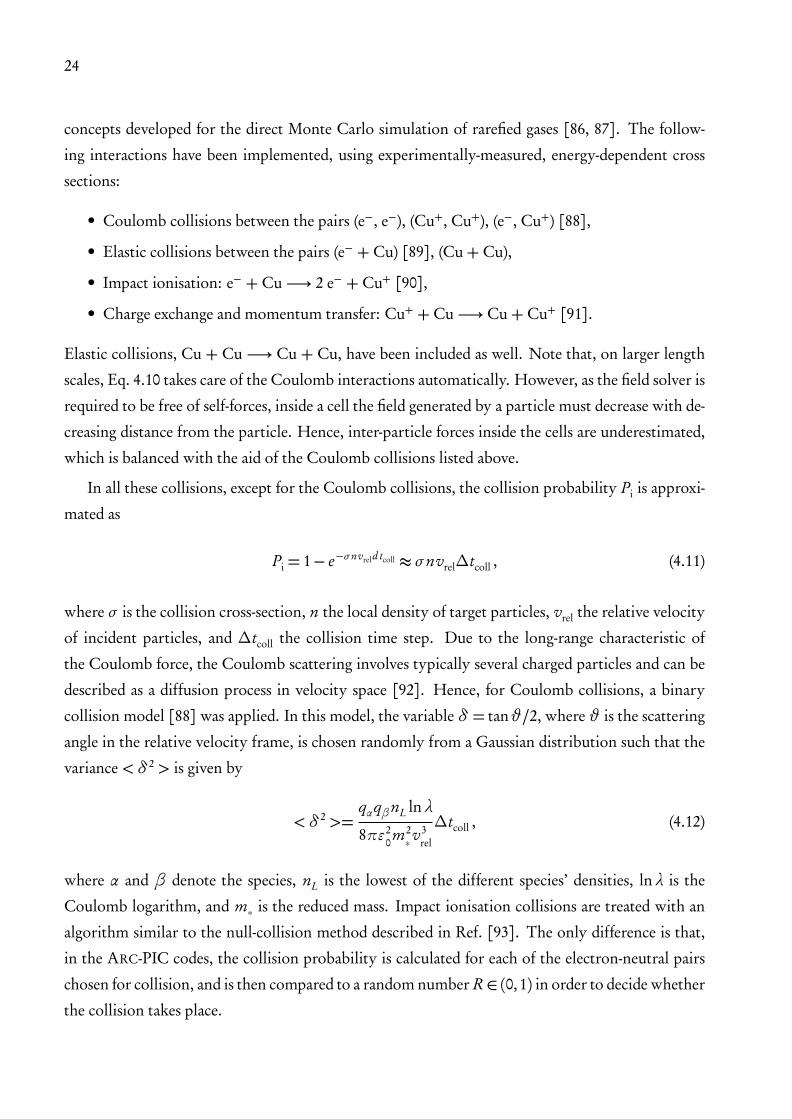
concepts developed for the direct Monte Carlo simulation of rarefied gases [86, 87]. The follow-

ing interactions have been implemented, using experimentally-measured, energy-dependent cross

sections:

• Coulomb collisions between the pairs (e−, e−), (Cu+, Cu+), (e−, Cu+) [88],

• Elastic collisions between the pairs (e− + Cu) [89], (Cu + Cu),

• Impact ionisation: e− + Cu −→ 2 e− + Cu+ [90],

• Charge exchange and momentum transfer: Cu+ + Cu −→ Cu + Cu+ [91].

Elastic collisions, Cu + Cu −→ Cu + Cu, have been included as well. Note that, on larger length

scales, Eq. 4.10 takes care of the Coulomb interactions automatically. However, as the field solver is

required to be free of self-forces, inside a cell the field generated by a particle must decrease with de-

creasing distance from the particle. Hence, inter-particle forces inside the cells are underestimated,

which is balanced with the aid of the Coulomb collisions listed above.

In all these collisions, except for the Coulomb collisions, the collision probability Pi is approxi-

mated as

Pi = 1− e−σnvreld tcoll ≈ σnvrel∆tcoll , (4.11)

where σ is the collision cross-section, n the local density of target particles, vrel the relative velocity

of incident particles, and ∆tcoll the collision time step. Due to the long-range characteristic of

the Coulomb force, the Coulomb scattering involves typically several charged particles and can be

described as a diffusion process in velocity space [92]. Hence, for Coulomb collisions, a binary

collision model [88] was applied. In this model, the variable δ = tanϑ/2, where ϑ is the scattering

angle in the relative velocity frame, is chosen randomly from a Gaussian distribution such that the

variance <δ2 > is given by

<δ2 >=qαqβnL lnλ

8πǫ20m2∗v

3rel

∆tcoll , (4.12)

where α and β denote the species, nL is the lowest of the different species’ densities, lnλ is the

Coulomb logarithm, and m∗ is the reduced mass. Impact ionisation collisions are treated with an

algorithm similar to the null-collision method described in Ref. [93]. The only difference is that,

in the ARC-PIC codes, the collision probability is calculated for each of the electron-neutral pairs

chosen for collision, and is then compared to a random number R ∈ (0,1) in order to decide whether

the collision takes place.

25

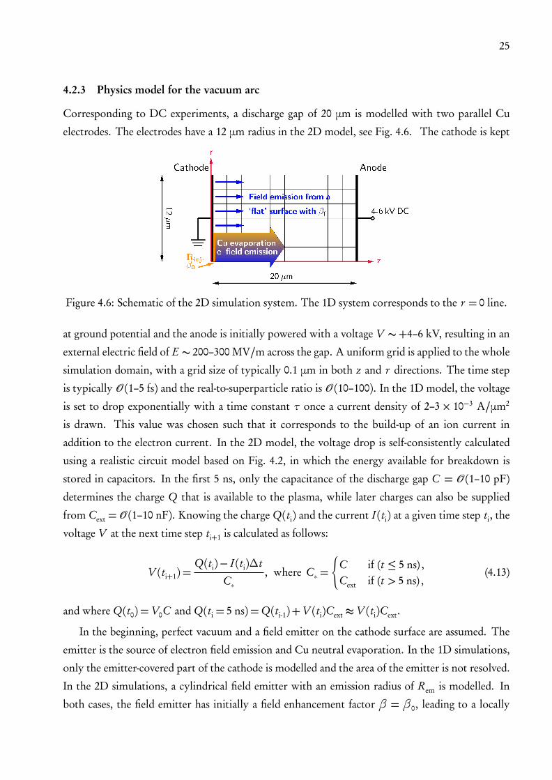
4.2.3 Physics model for the vacuum arc

Corresponding to DC experiments, a discharge gap of 20 µm is modelled with two parallel Cu

electrodes. The electrodes have a 12 µm radius in the 2D model, see Fig. 4.6. The cathode is kept

Figure 4.6: Schematic of the 2D simulation system. The 1D system corresponds to the r = 0 line.

at ground potential and the anode is initially powered with a voltage V ∼+4–6 kV, resulting in an

external electric field of E ∼ 200–300 MV/m across the gap. A uniform grid is applied to the whole

simulation domain, with a grid size of typically 0.1 µm in both z and r directions. The time step

is typically O (1–5 fs) and the real-to-superparticle ratio is O (10–100). In the 1D model, the voltage

is set to drop exponentially with a time constant τ once a current density of 2–3× 10−3 A/µm2

is drawn. This value was chosen such that it corresponds to the build-up of an ion current in

addition to the electron current. In the 2D model, the voltage drop is self-consistently calculated

using a realistic circuit model based on Fig. 4.2, in which the energy available for breakdown is

stored in capacitors. In the first 5 ns, only the capacitance of the discharge gap C = O (1–10 pF)

determines the charge Q that is available to the plasma, while later charges can also be supplied

from Cext = O (1–10 nF). Knowing the charge Q(ti) and the current I (ti) at a given time step ti, the

voltage V at the next time step ti+1 is calculated as follows:

V (ti+1) =Q(ti)− I (ti)∆t

C∗, where C∗ =

(

C if (t ≤ 5 ns) ,

Cext if (t > 5 ns) ,(4.13)

and where Q(t0) =V0C and Q(ti = 5 ns) =Q(ti-1)+V (ti)Cext ≈V (ti)Cext.

In the beginning, perfect vacuum and a field emitter on the cathode surface are assumed. The

emitter is the source of electron field emission and Cu neutral evaporation. In the 1D simulations,

only the emitter-covered part of the cathode is modelled and the area of the emitter is not resolved.

In the 2D simulations, a cylindrical field emitter with an emission radius of Rem is modelled. In

both cases, the field emitter has initially a field enhancement factor β = β0, leading to a locally

26

enhanced field of Eloc = β0E . As the emitter also evaporates, the erosion of the emitter is taken

into account by linearly reducing β with the atoms evaporated; here it is assumed that the field

enhancement factor represents the height to radius aspect ratio of the field emitter [29, 94]. Once

a threshold electron field emission current density jmelt is exceeded, the ‘melting’ of the emitter

takes place; this sets β = 1 in the 1D case and β = βf (see below) in the 2D case. For a large

enough (i.e. classically treatable) tip-like Cu protrusion jmelt = O (1012–1013 A/m2) can be estimated

based on Joule heating. Since in the 2D model Rem is typically O (∆z), in practice the radius of

particle injection Rinj can be chosen to be slightly bigger than Rem to ensure numerical stability. In

addition, in the 2D model, field emission can also occur at the ‘flat’ cathode surface with βf. In all

cases, Fowler-Nordheim emission is applied only up to Eloc = 12 GV/m, which is the validity range

for pure field emission [39]; above 12 GV/m, a constant extrapolation of the curve is used.

In reality, the evaporation of atoms from the emitter is due to a complex interplay of different

thermal and field-related processes [32]. In lieu of a self-consistent, ab initio calculation of evapora-

tion rates via MD simulations [32], a phenomenological evaporation scheme has been used in the

PIC models. Motivated by the fact that the high local field can result in a high enough electron field

emission current density to heat up a thin emitter significantly [33], ‘field assisted thermal evap-

oration’ is assumed that follows the field emission in a constant ratio rCu/e. This is based on MD

simulations [32, 33], which show that sharp field emitter tips, that are heated by the electron cur-

rent, can lead to enhanced atom emission compared to the pure low-temperature field evaporation

of ions [95].

In addition to field emission and neutral evaporation from the field emitter, different sputtering

processes can take place at the electrodes and serve as further sources of electrons and neutrals:

• Cu and Cu+ impinging at either electrode can sputter Cu with an experimentally measured,

energy dependent sputtering yield [96].

• Via MD simulations, plasma ions that are accelerated over the sheath and impinge at the

cathode with a high flux were shown to lead to a heat spike sputtering (see Sec. 5.4). As

a result, the sputtering yield is enhanced compared to the above mentioned experimentally

measured yield. Thus in PIC, above a Cu+ flux of 6× 1023 1/cm2/s incident to the cathode,

an average sputtering yield of Y = 1000 is applied (cf. Fig. 5.8). Note that this enhanced

sputtering yield is only applicable for high-energy ions in the early stage of arc burning, which

shall be discussed in detail in Sec. 5.4.

• High-energy ions can also cause a non-negligible secondary electron yield (SEY) at the cath-

ode. Therefore, above a Cu+ impact energy of 100 eV, a SEY of 0.5 is applied (an estimate

based on [97]).

27

Thus, the only source of Cu+ ions in the model is impact ionisation collisions; all particles

that are injected from the boundaries are either electrons or Cu neutrals. The injection of a given

particle p is carried out in a Gaussian distribution around the velocity vp

th=Æ

Tp/mp :

vpz=±

Æ

−2 ln r1 vp

th, (4.14a)

vpr=Æ

−2 ln r2 cos(2πr3)vp

th, (4.14b)

vp

ϑ=Æ

−2 ln r2 sin(2πr3)vp

th, (4.14c)

where r1, r2, and r3 ∈ [0,1] are random numbers and the plus and minus sign is applied for an

injection from the cathode and anode, respectively. The injection temperatures Tp can be adjusted.

4.3 MOLECULAR DYNAMICS SIMULATIONS

The molecular dynamics method [98] is a suitable choice whenever one is interested in gaining mi-

croscopic information on how the phase space variables of particles (atoms or molecules) in a given

system evolve; macroscopic information such as energy, temperature, and pressure can be obtained

through the formalism of a thermodynamic ensemble, by calculating time averaged quantities us-

ing the ergodic hypothesis. Widely applied in materials science and chemistry, one advantage of the

MD method is that it can describe crystal defects and treat collision cascades; a perfect combination

for simulating the breakdown-caused surface damage on the cathode.

For the Cu surface damage simulations presented in VI, the fully parallel PARCAS [99] code has

been used. Single crater formation events have been simulated with up to 2000 processors, total run

times of up to 200000 h, and system sizes of up to 20 million atoms. The techniques used within

PARCAS for this purpose are described below.

4.3.1 Solving the equations of motion

Given that PARCAS is based on the classical MD approach [98], it solves Newton’s equation as an

equation of motion for each atom p in the system:

Fp = mpap , (4.15)

where Fp is the force acting on the atom, mp is the atom’s mass and ap the resulting acceleration.

Since MD treats only the atoms of a lattice, but not the electrons, information on both the inter-

atomic forces and the close-to-equilibrium electronic effects is comprised in the potential energy V

28

that determines the force which an atom at position rp is subject to:

Fp =−(∇V )|rp. (4.16)

Contrary to PIC, MD has to track small displacements in the atomic positions. The algorithm

used in PARCAS for solving these equations of motion is the Gear5-algorithm [98], a fifth-order

predictor-corrector algorithm, in which the solution is first ‘guessed’ (predicted) and then corrected

to achieve the desired accuracy. Knowing the particle’s position rp, velocity vp, and acceleration

ap at a given time step ti, the form of these functions at the next time step ti+1 = ti +∆t is first

approximated with a fifth-order Taylor polynomial,

rapproxp

(ti+1) = rp(ti)+ vp(ti)∆t +ap(ti)

2!∆t 2+

r(3)p(ti)

3!∆t 3+

r(4)p(ti)

4!∆t 4+

r(5)p(ti)

5!∆t 5 , (4.17)

obtaining also vapproxp

(ti+1) and aapproxp

(ti+1) accordingly. On the other hand, the force and the ac-

celeration acting on the particle at the updated position rapproxp

(ti+1) can be calculated via Eqs. 4.16

and 4.15, resulting in a more accurate, ‘corrected’ acceleration acorrp(ti+1). Then the correction term

∆ap(ti+1) = acorrp(ti+1)− aapprox

p(ti+1) is used to calculate the corrected vcorr

p(ti+1) and rcorr

p(ti+1).

4.3.2 High energy effects: choice of time step and potential

The potential describing inter-atomic interactions is of central importance in MD (cf. Eq. 4.16) and

must therefore by carefully chosen/constructed depending on the physics problem in question.

Some important factors that need to be taken into account for the simulation of surface modifica-

tion caused by the breakdown of Cu are (i) the high flux of impinging ions, to be taken into account

in the time step and (ii) high-energy effects, to be taken into account in the potential.

The adaptive time step algorithm used in PARCAS [100] ensures that the time step ∆t is suit-

ably chosen for simulations of far-from-equilibrium events such as collision cascades. When ener-

getic particles are present,∆t is decreased to guarantee sufficient accuracy (cf. Eq. 4.17) and energy

conservation, and is increased for computational time saving purposes when the system is close to

equilibrium. Due to the high flux of plasma ions incident on the cathode, the impact time intervals

were as short as O (1–100 fs); in comparison, a typical MD time step is O (1 fs). Thus, special care

had to be taken that there are always at least three time steps simulated between each impact event.

The impact times were selected randomly from a Poisson distribution, with an average flux of about

1025 ions/cm2/s (calculated with PIC simulations).

The well-tested potential by Sabochick and Lam [101–104], based on the embedded-atom

method (EAM) [105, 106], was used for modelling the inter-atomic interactions in Cu. In a lattice,

29

long-range interactions are screened and thus in MD it is sufficient to consider only interactions be-

tween close neighbours. Therefore it is usually convenient to divide any N-body potential V into

contributions coming from single particle potentials V1, pair potentials V2, three-body potentials

V3, etc.:

V =N∑

i=1

V1(ri)+N∑

i=1

N∑

j=i

V2(ri,rj)+N∑

i=1

N∑

j=i

N∑

k= j

V3(ri,rj,rk)+ ... , (4.18)

where the first term V1 is only present in case of an external field and the pair potential V2 depends

only on the distance rij = |ri− rj| between the pair. In practice, the summation is carried out only

over atoms that are located within a cut-off radius. Well-suited for the modelling of metals with

a face-centred cubic (FCC) crystal structure, the EAM formalism uses the fact that the electron

density uniquely determines the potential in a solid [107] and thus the atoms of a solid can be

treated as an ‘impurity’ embedded in a sea of electrons. In this approach, the total energy Etot of

the system is expressed as a sum over atom pairs i and j of the short-range pair potential Vij and the

embedding energy Fi that is a functional of the electron charge density ρj :

Etot =∑

i

Fi

∑

j

i 6= j

ρj(rij)

+1

2

∑

i , j

i 6= j

Vij(rij) . (4.19)

Regarding high-energy effects, techniques such as energy loss to electrons and repulsive po-

tentials suitable for the simulation of energetic ion interactions with materials [103, 108] were

used. Energy loss to electrons was added as a frictional force slowing down all atoms with a kinetic

energy above that of normal thermal motions [100]. The magnitude of the force was obtained

from the SRIM computer code [109]. The repulsive potential was modified to the Ziegler-Biersack-

Littmark universal potential for inter-atomic separations that are clearly smaller than the equilib-

rium one [110].

4.3.3 Temperature control and boundary conditions

For energy to be conserved, usually a microcanonical, isolated system is modelled. However, when

simulating collision cascades, the system is interacting with its surroundings; the environment

serves as a heat bath of temperature T0, absorbing the heat produced during bombardment. To

avoid unphysical heating in the system, the temperature T of the system has to be adjusted.

In the bombardment simulations in publication VI, a temperature control method after Berend-

sen et al. [111] was utilised. With this method, a friction term is added to the equation of motion

30

to adjust the system temperature T to the temperature of the heat bath T0 within a time constant

τ = 1/(2γ ) :

Fp = mpap+mpvpγ

�

T0

T− 1

�

. (4.20)

In practise, this is implemented by re-scaling the atom velocities by the factor

λ=

s

1+∆t

τ

�

T0

T− 1

�

(4.21)

at each time step∆t .

The simulation system was assumed to be placed in an ambient temperature of T0 = 300 K,

to which the whole system was thermally relaxed within 1 ps prior to any bombardment. Then,

in one direction, a layer of one cell was fixed at the bottom of the lattice to mimic an underlying

bulk, while bombardment occurred at the top of the lattice. In the perpendicular plane, periodic

boundary conditions were applied. The Berendsen temperature control was applied in a layer of

five cells above the fixed layer as well as at the periodic boundaries.

5 From vacuum arc initiation to extinction

Different stages of the vacuum arc can be experimentally observed with the DC setup: field emis-

sion, breakdown, and resulting surface damage. However, the connection between these different

observations remains to be established in theory. From plasma evolution to the extinction of the

arc — several methods have been used to better understand the different stages and their connection.

The central findings of this thesis are described below.

A crucial element in this study is the modelling of plasma initiation in vacuum arcs, because it

provides a link between field emission and arc development, and thus sub-micron and macroscopic

scales. Moreover, it allows for interrelating theory and measurements in several aspects. Specifically,

one aim is to understand how the transition from field emission to a developed arc takes place and

how the arc can maintain itself. Studying the surface damage both theoretically and experimentally

is also important because here an almost direct comparison between theory and ‘real life’ is possible.

Finally, any information, whether obtained through experiments or theory, that bridges the gap

between DC and RF vacuum arcs is one step on the way to understanding the connection between

the two.

5.1 VACUUM ARC INITIATION

The starting point for the model of plasma initiation in vacuum arcs lies in the experimental ev-

idence of typical field emission parameters measured prior to breakdown. For processed Cu, the

field enhancement factor varies typically in the range β ∼ 30–70, and always such that the local

field leading to breakdown is around Eloc = 10–11 GV/m [67]. The corresponding emission areas

(cf. Eq. 3.1) covering about four orders of magnitude, Aem = O (10−20–10−16) m2 [26], indicate that

electron emission is initially concentrated to a nano-scale region.

The 1D and 2D plasma models are based on two assumptions. Firstly, the existence of a field

emitter on the cathode surface is postulated, which is the source of electron field emission with

a β typical of experiments; in the 2D model, even the emission radii (down to 100 nm) can be

resolved. Secondly, a more crucial assumption is that the emitter also evaporates neutrals and that

this evaporation is proportional to the field emission, with the constant of proportionality being

rCu/e. In the model, the evaporated neutrals are the first atoms that appear in the discharge gap;

without these atoms, no vacuum arc would develop. Thus the time-to-breakdown is expected to

have a distinct dependency on the strength of the neutral source; this dependency is discussed in

Sec. 5.3.

31

32

Two requirements for plasma build-up1 have been identified based on the 1D model in II. For

the plasma to build up, the right combination of electrons and Cu neutrals needs to be present in

the discharge gap. Firstly, field emission needs to be initially ‘strong’ enough in order to overcome

the space charge screening of the potential. The ‘strength’ of the field emission can be measured in

terms of jFN, or alternatively, in terms of Eloc (cf. Eq. 3.1). Simulations with different combinations

of an initialβ and an external electric field E showed that, independent of the strength of the neutral

source, no ionisation avalanche (see next paragraph), and thus no plasma, could be produced with

Eloc ® 8 GV/m. However, when starting initially from Eloc ¦ 10 GV/m, a slowly but steadily

growing field emission current density was observed (as will be seen later in Fig. 5.2). This slowly

but steadily growing current density is due to the first ionisations occurring in the system that start

to reduce the space charge screening of the potential, and hence, lead to a rising current density.

If a strong enough neutral source is also present, this growing field emission will lead to an

ionisation avalanche. Since neutrals move very slowly compared to the electrons, they accumulate

over the field emitter forming a ‘cloud’ of neutral gas. The ionisation avalanche or ‘runaway’ occurs

when the neutral density becomes high enough so that on average the electron mean free path of

the impact ionisation, lmfp = 1/(σnCu), becomes smaller than the system length lsys. Note that

densities can vary by orders of magnitude over the system length; typically a local density of nCu ∼1018 1/cm3 close to the emitter is sufficient to lead to a runaway. Once this critical neutral density

is reached, plasma formation is unavoidable: ions impinging at the cathode will sputter additional

neutrals, leading to a further increase in neutral density, which then again increases ionisation,

sputtering, and so forth.

The identified two requirements together indicate also that the experimentally observed break-

down threshold of Eloc = 10–11 GV/m might indeed be a material-dependent parameter that is

determined by space-charge effects and ionisation rates in the field emission stage.

5.2 EARLY PLASMA DEVELOPMENT

The above observations reveal the necessary conditions for a vacuum arc, i.e. for a plasma to be

initiated: the presence of a sufficiently strong electron and neutral source. However, they don’t

explain how exactly field emission turns into a developed arc when these conditions are fulfilled.

During its early development, the vacuum arc goes through different stages that were studied in

detail in III. Snapshots of these stages are shown in Fig. 5.1. Two ‘transitions’ can be identified:

firstly, a faster transition that turns a strong field emission into a ‘local arc plasma’ above the field

1To distinguish between field emission and arc burning stages, in this thesis, the term ‘plasma’ is devoted to thatstate of matter in the discharge gap which is quasi-neutral and where a plasma sheath is present.

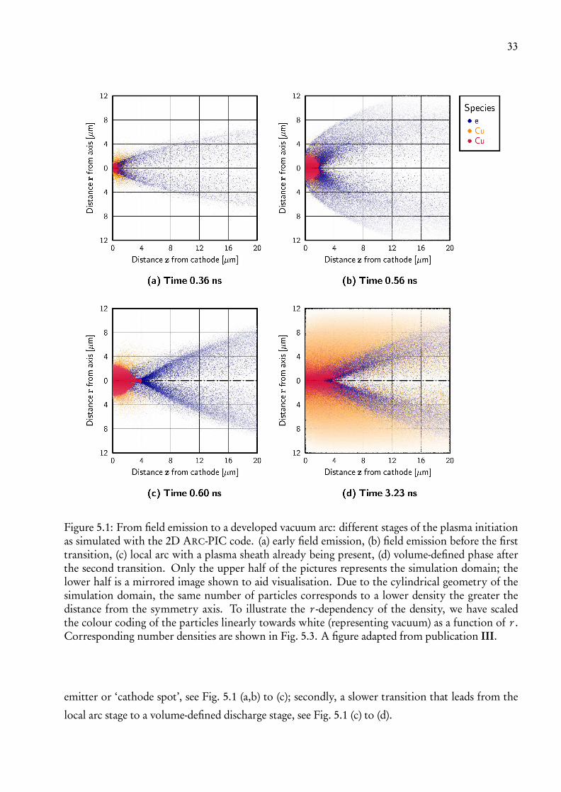
33

Figure 5.1: From field emission to a developed vacuum arc: different stages of the plasma initiationas simulated with the 2D ARC-PIC code. (a) early field emission, (b) field emission before the firsttransition, (c) local arc with a plasma sheath already being present, (d) volume-defined phase afterthe second transition. Only the upper half of the pictures represents the simulation domain; thelower half is a mirrored image shown to aid visualisation. Due to the cylindrical geometry of thesimulation domain, the same number of particles corresponds to a lower density the greater thedistance from the symmetry axis. To illustrate the r -dependency of the density, we have scaledthe colour coding of the particles linearly towards white (representing vacuum) as a function of r .Corresponding number densities are shown in Fig. 5.3. A figure adapted from publication III.

emitter or ‘cathode spot’, see Fig. 5.1 (a,b) to (c); secondly, a slower transition that leads from the

local arc stage to a volume-defined discharge stage, see Fig. 5.1 (c) to (d).

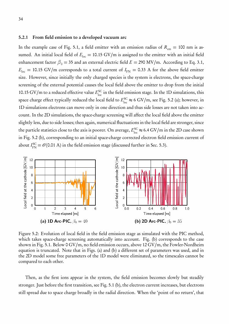
34

5.2.1 From field emission to a developed vacuum arc

In the example case of Fig. 5.1, a field emitter with an emission radius of Rem = 100 nm is as-

sumed. An initial local field of Eloc = 10.15 GV/m is assigned to the emitter with an initial field

enhancement factor β0 = 35 and an external electric field E = 290 MV/m. According to Eq. 3.1,

Eloc = 10.15 GV/m corresponds to a total current of IFN = 0.33 A for the above field emitter

size. However, since initially the only charged species is the system is electrons, the space-charge

screening of the external potential causes the local field above the emitter to drop from the initial

10.15 GV/m to a reduced effective value ESCloc

in the field emission stage. In the 1D simulations, this

space charge effect typically reduced the local field to ESCloc≈ 6 GV/m, see Fig. 5.2 (a); however, in

1D simulations electrons can move only in one direction and thus side losses are not taken into ac-

count. In the 2D simulations, the space-charge screening will affect the local field above the emitter

slightly less, due to side losses; then again, numerical fluctuations in the local field are stronger, since

the particle statistics close to the axis is poorer. On average, ESCloc≈ 6.4 GV/m in the 2D case shown

in Fig. 5.2 (b), corresponding to an initial space-charge corrected electron field emission current of

about I SCFN= O (0.01 A) in the field emission stage (discussed further in Sec. 5.3).

Figure 5.2: Evolution of local field in the field emission stage as simulated with the PIC method,which takes space-charge screening automatically into account. Fig. (b) corresponds to the caseshown in Fig. 5.1. Below 0 GV/m, no field emission occurs, above 12 GV/m, the Fowler-Nordheimequation is truncated. Note that in Figs. (a) and (b) a different set of parameters was used, and inthe 2D model some free parameters of the 1D model were eliminated, so the timescales cannot becompared to each other.

Then, as the first ions appear in the system, the field emission becomes slowly but steadily

stronger. Just before the first transition, see Fig. 5.1 (b), the electron current increases, but electrons

still spread due to space charge broadly in the radial direction. When the ‘point of no return’, that

35

is the condition for an ionisation avalanche as described in Sec. 5.1, is reached, suddenly more and

more ions are produced. Since electrons move fast, a quasi-neutral plasma can be established on a

sub-nanosecond timescale. As a consequence of quasi-neutrality and the presence of an absorbing

boundary, a plasma sheath forms above the cathode and the ion flow towards the cathode is facil-

itated, resulting in a rise in total current. Also electrons exiting this local arc plasma towards the

anode are now much more focussed, see Fig. 5.1 (c). Note that these focussed electrons carry most

of the plasma current and thus, if the anode is close enough and the electron current density is high

enough, an anode spot could develop and anode material could be evaporated.

After this first transition, neutrals slowly start to fill the discharge gap. Neutrals accumulate in

the gap due to their comparatively long travel time through the gap. The timescale of this accu-

mulation depends partly on the strength of the neutral source, which is at this stage determined by

sputtering. However, the average travel time is mainly given by the injection temperature of the

neutrals assumed in the model, which influences the timescale of accumulation largely. In the case

of Fig. 5.1, the neutral injection temperature (cf. Eq. 4.14) was set to TCu = 14.5 eV, and resulted in

a filling time of about 4 ns. By the term ‘filling time’, we mean the time that is required to establish

an equilibrium between neutrals entering and exiting the system. TCu was chosen such that it would

match the typical temperature of sputtered atoms, which is O (10 eV) [112], so in terms of the ref-

erence temperature Tref = 2900 eV, to which all temperatures were rescaled in our code, we picked

TCu = 0.005×Tref. The choice of Te− is less critical, since electrons are immediately accelerated after

injection, and hence, we chose a reasonable value of Te− = 10−4×Tref = 0.29 eV.

Finally, the vacuum arc enters the stage of a volume-defined discharge, see Fig. 5.1 (d), in which

the plasma can fill in principle the whole discharge gap, provided that (i) there is enough time to

reach this stage and (ii) the neutral density becomes high enough along the symmetry axis to lead

to sufficient ionisation.

5.2.2 A self-maintaining plasma

In the region where a plasma is present, the plasma sheath, see Fig. 5.3, concentrates the external

potential into a small layer above the plasma-surface interface. This leads to a local enhancement of

the external electric field of up to 5–6 GV/m, see Fig. 5.4, above the original cathode spot in the case

of Fig. 5.1. Since the thickness of the plasma sheath is of the order of λD, the field enhancement due

to the plasma sheath is roughly given by the ratio Lpl/λD, where Lpl is the ‘length’ of the plasma.

Hence, the sheath can result in a field enhancement — at least above the original cathode spot

— that is able to maintain the level of electron emission even without any other source of field

enhancement. Combining this with the fact that the neutral sputtering, coming from plasma ions

36

Figure 5.3: Typical number densities and potential profiles of the arc shown in Fig. 5.1 after thefirst transition and for three different radial distances in the system. Note that close to the axis thesheath is concentrated into a sub-micron region of ∼ 0.2–0.3 µm above the cathode, and that inthe first ∼ 3–4 µm beyond the sheath the potential is flat, which is where the plasma is located, cf.Fig. 5.1. A figure adapted from publication III.

bombarding the cathode, leads to a volume-defined discharge phase in which the source of ions is

automatically provided, it can be concluded that the plasma is self-maintaining as long as energy for

the arc burning is available. Thus the presence of the plasma creates an environment that provides

a sufficient flow of both electrons and neutrals from the cathode into the plasma in order to make

the burning of the vacuum arc, once ignited, essentially unstoppable.

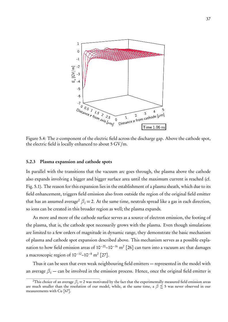
37

Figure 5.4: The z-component of the electric field across the discharge gap. Above the cathode spot,the electric field is locally enhanced to about 5 GV/m.

5.2.3 Plasma expansion and cathode spots

In parallel with the transitions that the vacuum arc goes through, the plasma above the cathode

also expands involving a bigger and bigger surface area until the maximum current is reached (cf.

Fig. 5.1). The reason for this expansion lies in the establishment of a plasma sheath, which due to its

field enhancement, triggers field emission also from outside the region of the original field emitter

that has an assumed average2 βf = 2. At the same time, neutrals spread like a gas in each direction,

so ions can be created in this broader region as well; the plasma expands.

As more and more of the cathode surface serves as a source of electron emission, the footing of

the plasma, that is, the cathode spot necessarily grows with the plasma. Even though simulations

are limited to a few orders of magnitude in dynamic range, they demonstrate the basic mechanism

of plasma and cathode spot expansion described above. This mechanism serves as a possible expla-

nation to how field emission areas of 10−20–10−16 m2 [26] can turn into a vacuum arc that damages

a macroscopic region of 10−12–10−8 m2 [27].

Thus it can be seen that even weak neighbouring field emitters — represented in the model with

an average βf — can be involved in the emission process. Hence, once the original field emitter is

2This choice of an average βf = 2 was motivated by the fact that the experimentally measured field emission areasare much smaller than the resolution of our model, while, at the same time, a β ® 5 was never observed in ourmeasurements with Cu [67].

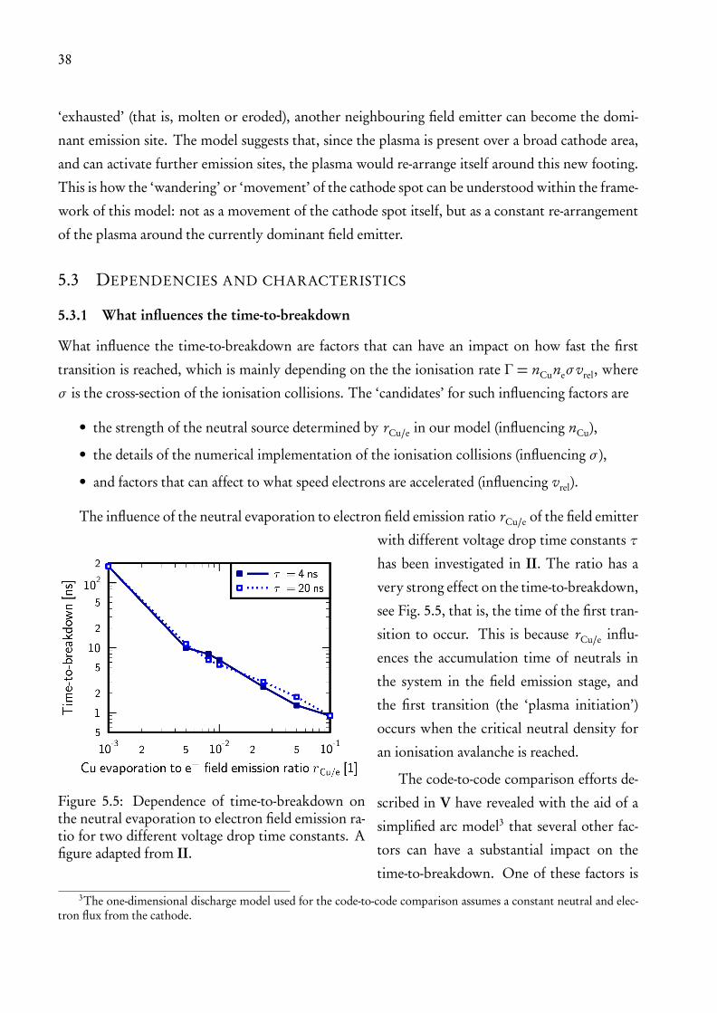
38

‘exhausted’ (that is, molten or eroded), another neighbouring field emitter can become the domi-

nant emission site. The model suggests that, since the plasma is present over a broad cathode area,

and can activate further emission sites, the plasma would re-arrange itself around this new footing.

This is how the ‘wandering’ or ‘movement’ of the cathode spot can be understood within the frame-

work of this model: not as a movement of the cathode spot itself, but as a constant re-arrangement

of the plasma around the currently dominant field emitter.

5.3 DEPENDENCIES AND CHARACTERISTICS

5.3.1 What influences the time-to-breakdown

What influence the time-to-breakdown are factors that can have an impact on how fast the first

transition is reached, which is mainly depending on the the ionisation rate Γ = nCuneσvrel, where

σ is the cross-section of the ionisation collisions. The ‘candidates’ for such influencing factors are

• the strength of the neutral source determined by rCu/e in our model (influencing nCu),

• the details of the numerical implementation of the ionisation collisions (influencing σ ),

• and factors that can affect to what speed electrons are accelerated (influencing vrel).

The influence of the neutral evaporation to electron field emission ratio rCu/e of the field emitter

Figure 5.5: Dependence of time-to-breakdown onthe neutral evaporation to electron field emission ra-tio for two different voltage drop time constants. Afigure adapted from II.

with different voltage drop time constants τ

has been investigated in II. The ratio has a

very strong effect on the time-to-breakdown,

see Fig. 5.5, that is, the time of the first tran-

sition to occur. This is because rCu/e influ-

ences the accumulation time of neutrals in

the system in the field emission stage, and

the first transition (the ‘plasma initiation’)

occurs when the critical neutral density for

an ionisation avalanche is reached.

The code-to-code comparison efforts de-

scribed in V have revealed with the aid of a

simplified arc model3 that several other fac-

tors can have a substantial impact on the

time-to-breakdown. One of these factors is

3The one-dimensional discharge model used for the code-to-code comparison assumes a constant neutral and elec-tron flux from the cathode.

39

the scheme used to interpolate in-between and extrapolate outside the available data points of

the energy-dependent cross-section of ionisation collisions; this scheme’s influence on the time-

to-breakdown is O (20 %). The specific numerical collision methods used as well as post-ionisation

energy disposal can also influence the result.

Related to PIC methodology, a zeroth order (constant) scheme for the interpolation of the elec-

tric field from grid points to particle positions has proven to have insufficient accuracy (at least for

the typical grid size used in the simulations). An insufficient accuracy in the field interpolation

shows directly in the electron acceleration close to the cathode, since in the sheath region the elec-

tric field has strong gradients. An inaccurate estimate of the electron acceleration carries over to

the relative velocity of electrons and neutrals in the impact ionisation, which in turn leads to an

inaccurate estimate of ionisation rates; as a result, the time-to-breakdown can be over- or underes-

timated significantly (O (100 %)). Moreover, an insufficient accuracy can also manifest itself in a

non-convergent solution.

Due to the non-linear nature of breakdowns, the exact details of the numerical model can influ-

ence quantitative simulation results (timescales). Nevertheless, good qualitative agreement of break-

down behaviour, potential, and densities was shown with two independent codes in V. Bearing this

in mind, quantitative results of both the 1D and the 2D plasma models should be understood as an

order-of-magnitude estimate.

5.3.2 Current-voltage characteristic, burning voltage, and energy balance

From knowing the evolution of the current-voltage characteristic of vacuum arcs, essential infor-

mation such as the energy consumption and the arc resistance can be extracted, information, that

is also extremely valuable from an experimental point of view. With the PIC models, the early

development (O (10 ns)) of this characteristic curve has been studied (the 1D model is limited to a

current-density–voltage characteristic). Two typical characteristics obtained with the 2D model are

presented in Fig. 5.6.

During the field emission phase, the current I rises rather slowly and the voltage V is almost

unaffected. The corresponding resistance R, if defined as R= dV /dI , is negative and rather large –

the discharge gap represents an open circuit. The negative resistance is due to a rising current with

dropping voltage.

As it can already be seen from Fig. 5.1, the first transition from field emission to a local vacuum

arc plasma happens very fast. What limits the current from rising further than 0.4 A in this case

is the amount of field emission electrons that can be supplied from the emitter. The total plasma

current coming from the emitter region is mainly electron current and thus determined by the

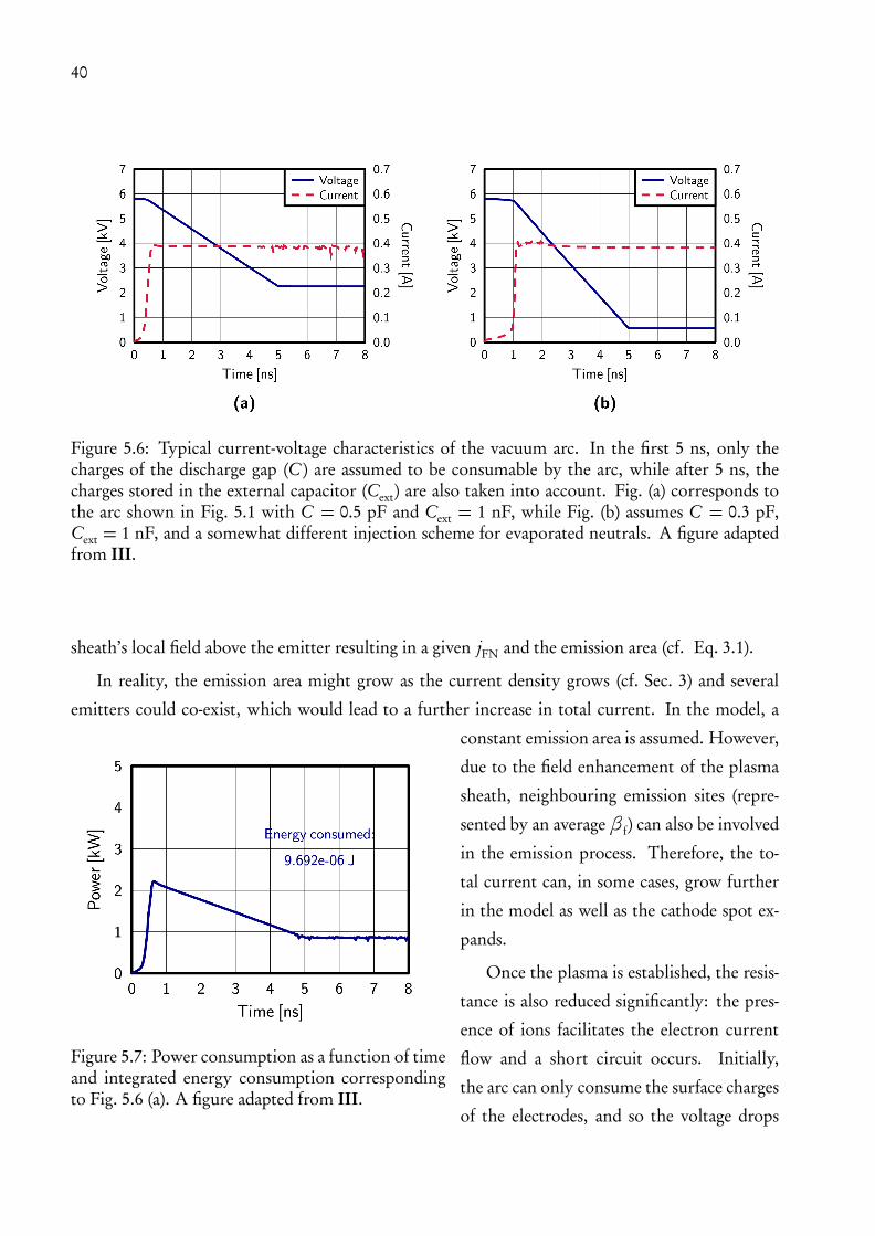
40

Figure 5.6: Typical current-voltage characteristics of the vacuum arc. In the first 5 ns, only thecharges of the discharge gap (C ) are assumed to be consumable by the arc, while after 5 ns, thecharges stored in the external capacitor (Cext) are also taken into account. Fig. (a) corresponds tothe arc shown in Fig. 5.1 with C = 0.5 pF and Cext = 1 nF, while Fig. (b) assumes C = 0.3 pF,Cext = 1 nF, and a somewhat different injection scheme for evaporated neutrals. A figure adaptedfrom III.

sheath’s local field above the emitter resulting in a given jFN and the emission area (cf. Eq. 3.1).

In reality, the emission area might grow as the current density grows (cf. Sec. 3) and several

emitters could co-exist, which would lead to a further increase in total current. In the model, a

Figure 5.7: Power consumption as a function of timeand integrated energy consumption correspondingto Fig. 5.6 (a). A figure adapted from III.

constant emission area is assumed. However,

due to the field enhancement of the plasma

sheath, neighbouring emission sites (repre-

sented by an averageβf) can also be involved

in the emission process. Therefore, the to-

tal current can, in some cases, grow further

in the model as well as the cathode spot ex-

pands.

Once the plasma is established, the resis-

tance is also reduced significantly: the pres-

ence of ions facilitates the electron current

flow and a short circuit occurs. Initially,

the arc can only consume the surface charges

of the electrodes, and so the voltage drops

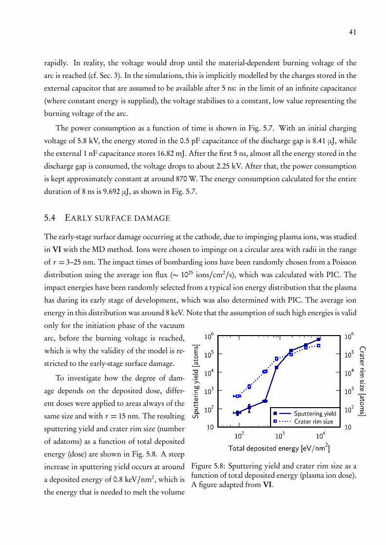
41

rapidly. In reality, the voltage would drop until the material-dependent burning voltage of the

arc is reached (cf. Sec. 3). In the simulations, this is implicitly modelled by the charges stored in the

external capacitor that are assumed to be available after 5 ns: in the limit of an infinite capacitance

(where constant energy is supplied), the voltage stabilises to a constant, low value representing the

burning voltage of the arc.

The power consumption as a function of time is shown in Fig. 5.7. With an initial charging

voltage of 5.8 kV, the energy stored in the 0.5 pF capacitance of the discharge gap is 8.41 µJ, while

the external 1 nF capacitance stores 16.82 mJ. After the first 5 ns, almost all the energy stored in the

discharge gap is consumed, the voltage drops to about 2.25 kV. After that, the power consumption

is kept approximately constant at around 870 W. The energy consumption calculated for the entire

duration of 8 ns is 9.692 µJ, as shown in Fig. 5.7.

5.4 EARLY SURFACE DAMAGE

The early-stage surface damage occurring at the cathode, due to impinging plasma ions, was studied

in VI with the MD method. Ions were chosen to impinge on a circular area with radii in the range

of r = 3–25 nm. The impact times of bombarding ions have been randomly chosen from a Poisson

distribution using the average ion flux (∼ 1025 ions/cm2/s), which was calculated with PIC. The

impact energies have been randomly selected from a typical ion energy distribution that the plasma

has during its early stage of development, which was also determined with PIC. The average ion

energy in this distribution was around 8 keV. Note that the assumption of such high energies is valid

Figure 5.8: Sputtering yield and crater rim size as afunction of total deposited energy (plasma ion dose).A figure adapted from VI.

only for the initiation phase of the vacuum

arc, before the burning voltage is reached,

which is why the validity of the model is re-

stricted to the early-stage surface damage.

To investigate how the degree of dam-

age depends on the deposited dose, differ-

ent doses were applied to areas always of the

same size and with r = 15 nm. The resulting

sputtering yield and crater rim size (number

of adatoms) as a function of total deposited

energy (dose) are shown in Fig. 5.8. A steep

increase in sputtering yield occurs at around

a deposited energy of 0.8 keV/nm2, which is

the energy that is needed to melt the volume

42

Figure 5.9: Early-stage cathode surface damage caused by energetic plasma ions. The atoms arecoloured according to the height above the surface, with dark yellow corresponding to the originalsurface position, and light yellow and red giving the positions of atoms above the surface. Theheight scale is given in ångström to the right. Note the sub-nanosecond timescale that justifies theassumption of energetic ions in the early stage of a vacuum arc. A figure adapted from VI.

into which the energy is deposited; thus this threshold energy marks a transition.

Below the transition threshold, the crater rim size increases non-linearly with energy; however,

the sputtered particles are mainly single atoms and the damage on the surface stays rather low. Since

ions impinge with high energies, their penetration depth is big (up to 8 nm) and each of the ions

causes a single heat spike4 event that can heat the sample locally to very high temperatures. Below

4A heat spike is a many-body collision cascade in which collisions occur so densely packed that they cannot betreated independently.

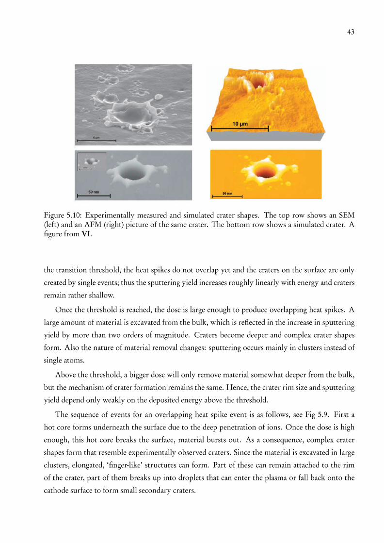
43

Figure 5.10: Experimentally measured and simulated crater shapes. The top row shows an SEM(left) and an AFM (right) picture of the same crater. The bottom row shows a simulated crater. Afigure from VI.

the transition threshold, the heat spikes do not overlap yet and the craters on the surface are only

created by single events; thus the sputtering yield increases roughly linearly with energy and craters

remain rather shallow.

Once the threshold is reached, the dose is large enough to produce overlapping heat spikes. A

large amount of material is excavated from the bulk, which is reflected in the increase in sputtering

yield by more than two orders of magnitude. Craters become deeper and complex crater shapes

form. Also the nature of material removal changes: sputtering occurs mainly in clusters instead of

single atoms.

Above the threshold, a bigger dose will only remove material somewhat deeper from the bulk,

but the mechanism of crater formation remains the same. Hence, the crater rim size and sputtering

yield depend only weakly on the deposited energy above the threshold.

The sequence of events for an overlapping heat spike event is as follows, see Fig 5.9. First a

hot core forms underneath the surface due to the deep penetration of ions. Once the dose is high

enough, this hot core breaks the surface, material bursts out. As a consequence, complex crater

shapes form that resemble experimentally observed craters. Since the material is excavated in large

clusters, elongated, ‘finger-like’ structures can form. Part of these can remain attached to the rim

of the crater, part of them breaks up into droplets that can enter the plasma or fall back onto the

cathode surface to form small secondary craters.

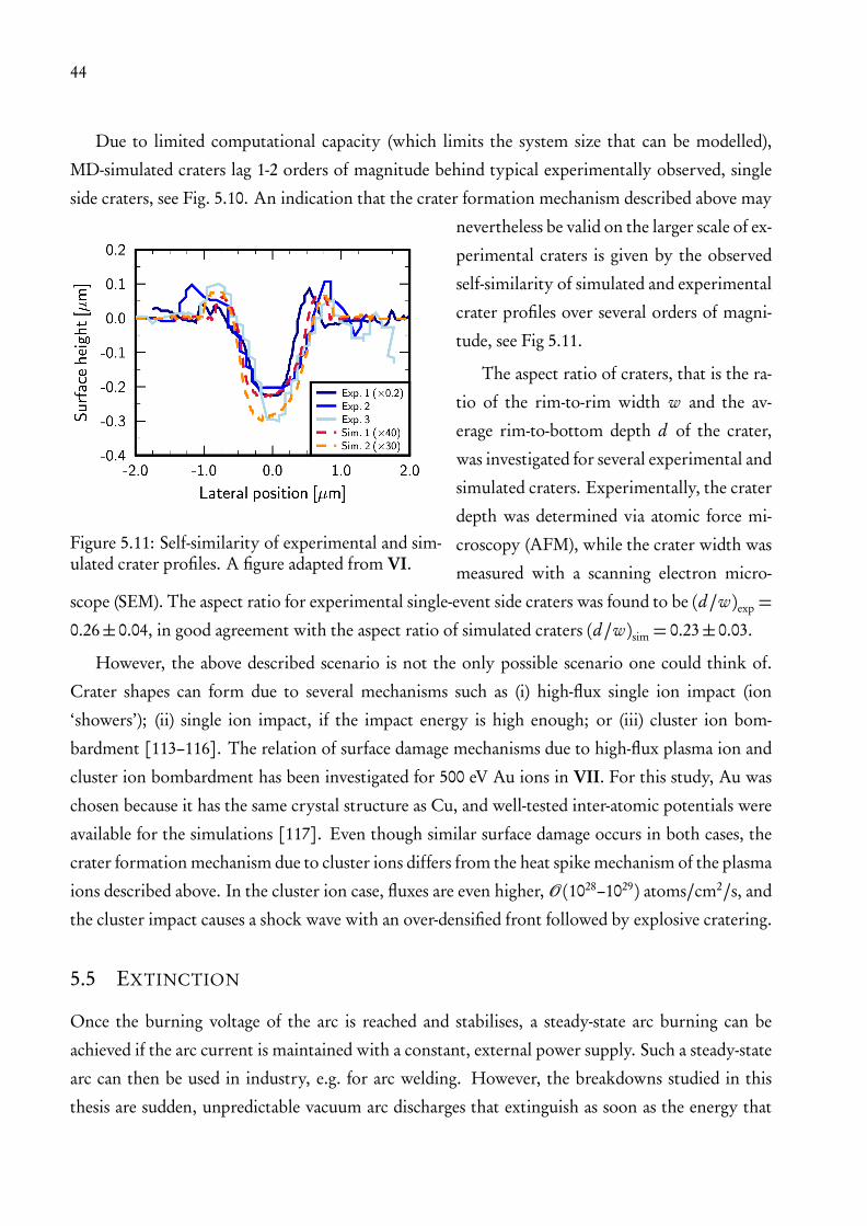
44

Due to limited computational capacity (which limits the system size that can be modelled),

MD-simulated craters lag 1-2 orders of magnitude behind typical experimentally observed, single

side craters, see Fig. 5.10. An indication that the crater formation mechanism described above may

Figure 5.11: Self-similarity of experimental and sim-ulated crater profiles. A figure adapted from VI.

nevertheless be valid on the larger scale of ex-

perimental craters is given by the observed

self-similarity of simulated and experimental

crater profiles over several orders of magni-

tude, see Fig 5.11.

The aspect ratio of craters, that is the ra-

tio of the rim-to-rim width w and the av-

erage rim-to-bottom depth d of the crater,

was investigated for several experimental and

simulated craters. Experimentally, the crater

depth was determined via atomic force mi-

croscopy (AFM), while the crater width was

measured with a scanning electron micro-

scope (SEM). The aspect ratio for experimental single-event side craters was found to be (d/w)exp =

0.26± 0.04, in good agreement with the aspect ratio of simulated craters (d/w)sim = 0.23± 0.03.

However, the above described scenario is not the only possible scenario one could think of.

Crater shapes can form due to several mechanisms such as (i) high-flux single ion impact (ion

‘showers’); (ii) single ion impact, if the impact energy is high enough; or (iii) cluster ion bom-

bardment [113–116]. The relation of surface damage mechanisms due to high-flux plasma ion and

cluster ion bombardment has been investigated for 500 eV Au ions in VII. For this study, Au was

chosen because it has the same crystal structure as Cu, and well-tested inter-atomic potentials were

available for the simulations [117]. Even though similar surface damage occurs in both cases, the

crater formation mechanism due to cluster ions differs from the heat spike mechanism of the plasma

ions described above. In the cluster ion case, fluxes are even higher, O (1028–1029) atoms/cm2/s, and

the cluster impact causes a shock wave with an over-densified front followed by explosive cratering.

5.5 EXTINCTION

Once the burning voltage of the arc is reached and stabilises, a steady-state arc burning can be

achieved if the arc current is maintained with a constant, external power supply. Such a steady-state

arc can then be used in industry, e.g. for arc welding. However, the breakdowns studied in this

thesis are sudden, unpredictable vacuum arc discharges that extinguish as soon as the energy that

45

was available in the system is consumed.

CLIC RF cavities are typically operated with ∼ 250 ns long pulses (∼ 150 ns flat top) that

store about 1–10 J energy [70], which gives an upper limit to the energy that can be consumed

by a discharge (cf. Sec. 4.1). In case of a breakdown, due to the high arc currents, the resonant

electromagnetic field in the cavity collapses on the ns timescale; the original pulse form can no

longer be maintained, power is no longer transmitted. With the field collapsing, also the boundary

conditions for the potential change rapidly, which makes the modelling of plasma initiation in an

RF cavity harder to capture than a DC breakdown. What is, however, known from the optical

spectroscopy of RF breakdowns, is that their light emission can last for 1–2 µs [53], and hence,

neutrals and ions are present in the system long after the RF pulse is gone.

In the DC case, there is no pulse form. However, the boundary conditions for the potential are

better-defined. Typical current-voltage characteristics measured with the DC setup are shown in

Fig. 5.12.

Figure 5.12: Current-voltage characteristics measured with the DC setup with different externalcapacitances corresponding to different energies stored in the capacitors. Note that the voltagesignal cannot be reliably measured once the low-voltage regime is reached; the negative voltage is anartifact of this. Oscillations on the current and the voltage signals are due to mechanical resonancesin the measurement system. A figure adapted from I.

The voltage drops exponentially with the time constant of the external RC-circuit. At the same

time, the current rises up to its maximum. Once the energy stored in the external capacitor is used

up, the voltage drops to zero. The current signal, however, can last up to a ∼ 1 µs longer, slowly

decreasing to zero. This is because once the voltage is off, the charged particles of the remaining

46

quasi-neutral gas are externally not accelerated anymore and can survive much longer in the dis-

charge gap. Fig. 5.12 (a) suggests a travel time of up to 1 µs and therefore an average ion velocity

of 20 µm/1 µs= 20 m/s for the slowest ions. Time-resolved optical spectroscopy measurements of

breakdowns generated with the DC setup confirm the presence of neutrals and ions in the system

for a total of 2–3 µs [53].

In summary, it can be concluded that in both the DC and RF cases the plasma extinguishes as

follows. Once the energy is consumed, the external voltage drops to zero. Electrons can no longer

be supplied to the plasma. Since electrons are much faster than ions, a part of them may escape the

plasma first, until an electrostatic equilibrium is reached. The remaining gas exhibits a rather long

decay process of cool-down, which can be detected through the light emission of neutrals and ions,

and the current signals that are seen long after the energy resources are depleted.

5.6 DC AND RF SCALING LAWS

While the investigation of DC vacuum arcs is by itself a well-defined problem with many potential

applications, since our primary interest is in RF breakdowns, we would also like to understand how

results obtained in the DC case translate to the RF case. Establishing scaling laws can help to resolve

this problem. Despite major differences between DC and RF breakdowns, several observations

indicate that the underlying physics has to be very similar in both cases.

The above mentioned optical spectroscopy results are only one example of how DC and RF

cases can be compared. Earlier measurements confirmed that in the DC case the breakdown prob-

ability scales with the saturated field in the same way as breakdown rate scales with accelerating

gradient in RF accelerating cavities [40]. The dependence was investigated for both Cu and Mo,

and in both DC and RF cases. The underlying scaling law turns out to be universally valid for both

DC and RF, but the scaling is different for Cu and Mo and is thus material dependent.

By studying then the DC energy dependence of breakdown properties in publication I, we have

established the scaling of the saturated field with the energy available for Cu and Mo, see Fig. 5.13.

Based on extensive Cu accelerating cavity testing, a similar scaling law between the accelerating

gradient Eacc and the pulse length τ for a constant breakdown rate was derived earlier: Eacc ∝τ−1/6 [9, 10]. Since the DC saturated field Esat and the RF accelerating gradient Eacc scale in the

same way with breakdown probability, and given that Esat corresponds to a constant breakdown

probability of about 10−2 [40], Esat can be directly translated to Eacc. In addition, the RF pulse

length τ can be related to the RF energy stored in a pulse WRF ∝ τV 2 ∝ τE2acc

, which can be

directly compared to the energy stored in DC WDC. Therefore, by replacing Eacc with Esat and

τ with WDC, the RF scaling law Eacc ∝ τ−1/6 takes in terms of DC variables the following form:

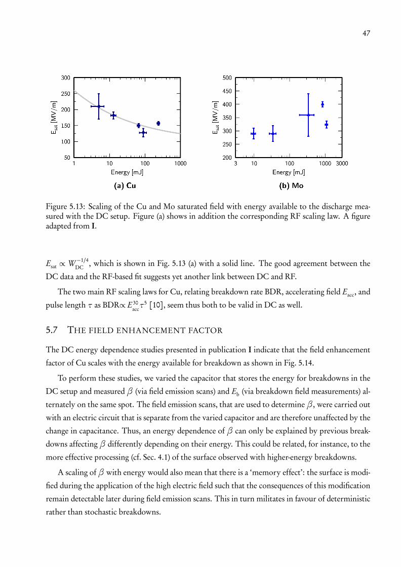
47

Figure 5.13: Scaling of the Cu and Mo saturated field with energy available to the discharge mea-sured with the DC setup. Figure (a) shows in addition the corresponding RF scaling law. A figureadapted from I.

Esat ∝W −1/4DC

, which is shown in Fig. 5.13 (a) with a solid line. The good agreement between the

DC data and the RF-based fit suggests yet another link between DC and RF.

The two main RF scaling laws for Cu, relating breakdown rate BDR, accelerating field Eacc, and

pulse length τ as BDR∝ E30accτ5 [10], seem thus both to be valid in DC as well.

5.7 THE FIELD ENHANCEMENT FACTOR

The DC energy dependence studies presented in publication I indicate that the field enhancement

factor of Cu scales with the energy available for breakdown as shown in Fig. 5.14.

To perform these studies, we varied the capacitor that stores the energy for breakdowns in the

DC setup and measured β (via field emission scans) and Eb (via breakdown field measurements) al-

ternately on the same spot. The field emission scans, that are used to determineβ, were carried out

with an electric circuit that is separate from the varied capacitor and are therefore unaffected by the

change in capacitance. Thus, an energy dependence of β can only be explained by previous break-

downs affecting β differently depending on their energy. This could be related, for instance, to the

more effective processing (cf. Sec. 4.1) of the surface observed with higher-energy breakdowns.

A scaling ofβwith energy would also mean that there is a ‘memory effect’: the surface is modi-

fied during the application of the high electric field such that the consequences of this modification

remain detectable later during field emission scans. This in turn militates in favour of deterministic

rather than stochastic breakdowns.

48

Figure 5.14: Energy dependence of the Cu field enhancement factor. A figure adapted from I.

In general, a dependence on the energy W ∝ E2 can also be translated to a dependence on the

electric field E , suggesting that β = β(W ) = β(E). Indeed, since a high electric field can lead

to a constant re-arrangement, growth or relaxation, of surface features (e.g. growth from voids is

demonstrated in [34]), a dependence of β on E cannot be excluded. If such a dependence existed,

Eq. 3.1 would have to be modified accordingly.

6 Conclusions and outlook

As a central part of this thesis, we have developed the 2D ARC-PIC code, and the physics model

incorporated in it, to study plasma initiation in Cu vacuum arcs. We identified the requirements for

plasma initiation as (i) a high enough initial local field of around 10 GV/m and (ii) a strong enough

neutral source during the field emission phase that can produce local neutral densities of the order

of 1018 1/cm3 in the vicinity of the field emitter.

From field emission to the early stage of arc burning, we could observe two transitions. Firstly,

a rapid transition from field emission to a local arc plasma that occurs due to a fast ionisation

avalanche and subsequent plasma sheath formation. During this process, both the total current and

the cathode area involved can grow several orders of magnitude. Secondly, a slower transition from

a local arc to a volume discharge can be seen as the discharge gap is steadily filled with neutrals.

Once the arc is initiated, it is self-maintaining through a combination of (i) the plasma sheath

that guarantees a sufficient electron supply from the cathode spot and (ii) intense sputtering due

to ion bombardment that ensures an adequate neutral supply. The cathode spot is thus ‘feeding’

the arc, even if the original field emitter is not present anymore. Our simulations have explicitly

shown how, due to the sheath, the cathode spot can spread sidewards, involving smaller field emitter

sites into the process of arc burning. Hence, the cathode spot also has the potential to ‘move’

to more dominant field emitter sites once the original field emitter is exhausted. Moreover, the

sidewards spreading gives a possible explanation of how the experimentally deduced field emission

areas of 10−20–10−16 m2 [26] can lead to the experimentally observed final damaged regions of 10−12–

10−8 m2 [27].

As a function of the neutral source strength during the field emission stage, we have given an

order-of-magnitude estimate of the time-to-breakdown. However, the time-to-breakdown can be

influenced by several factors in the numerical model. In this regard, our results of a code-to-code

comparison carried out with two independent codes using a simplified model have shown which

are the most important influencing factors and that the time-to-breakdown is reproducible, given

the same conditions.

Furthermore, we have self-consistently modelled the electric circuit of the DC setup in the

PIC simulations and have given thereby a qualitative prediction of the early-stage current-voltage

characteristic and the energy consumption, which can help to benchmark against experiments in

the future.

Coupled to PIC simulations, we have modelled the corresponding early-stage surface damage

49

50

with MD. Above a threshold deposited energy density of 0.8 keV/nm2, the sputtering yield in-

creases significantly. Above this threshold, sputtering occurs dominantly in clusters; finger-like

structures and complex crater shapes form. Our results have shown that the crater shapes of sim-

ulated and experimentally observed DC side craters are self-similar with the same crater depth-to-

width ratio of d/w ≈ 0.23 (sim) – 0.26 (exp). Despite producing similar crater shapes, the crater

formation mechanism due to high-flux single-ion bombardment was found to differ from the mech-

anism due to ion cluster bombardment.

We have also investigated the energy dependence of Cu and Mo breakdown properties experi-

mentally with the DC setup. The scaling of the Cu saturated field suggests that the RF scaling law

Eacc ∼ τ−1/6 might also be valid for DC. Furthermore, the observed scaling of the Cu field enhance-

ment factor with energy suggests a dynamic evolution ofβwith breakdowns occurring at different

electric fields and energies.

Several issues remain to be explored in the future. Firstly, the starting point to the studies

presented in this thesis is field emitters; how such field emitters are created, and what their field

enhancement is due to, is still unknown. Secondly, the plasma model could be refined by taking

into account thermal effects such as thermionic emission, the heating of the emitter, etc.; this,

however, would require more information about the properties of the field emitter. Thirdly, a

desirable future direction would be to achieve a better understanding of the connection between

DC and RF breakdowns as well as to perform more direct benchmarking between theory and

experiments, which is necessary in order to confirm fundamental assumptions in the theoretical

model.

Acknowledgements

I would like to thank Prof. Juhani Keinonen, head of the Department of Physics, for giving me

the opportunity to conduct research at the department and my supervisor Prof. Kai Nordlund

for seeing the potential in me and guiding me throughout the years. I thoroughly enjoyed the

helpful and interesting discussions I had with my project leader, Flyura Djurabekova PhD and all

my colleagues in this project, Leila, Aarne, Avaz, Juha, and Stefan.

I am grateful to my CERN supervisors Sergio Calatroni dott. and Mauro Taborelli PhD for

their help and the possibility to participate in the measurements. Walter Wuensch PhD, who was

a mentor to me not only in the physics-related questions, deserves my special thanks for all the

inspiring conversations and for always having time for me. Thanks to my colleagues and friends

Anita, Christina, Rocío, Tomoko, Jan, Markus, and Nick, I had a great time at CERN, both during

and outside working hours.

Above all, I would like to thank Prof. Ralf Schneider and Konstantin Matyash PhD who taught

me all I know about PIC, who were always there for me, and gave me much valuable advice.

I feel deep gratitude and love for my family who always gave me strength and support.

Financial support from the EuCARD project and the Magnus Ehrnrooth foundation is grate-

fully acknowledged.

Geneva, 6th November 2011

Helga Timkó

51

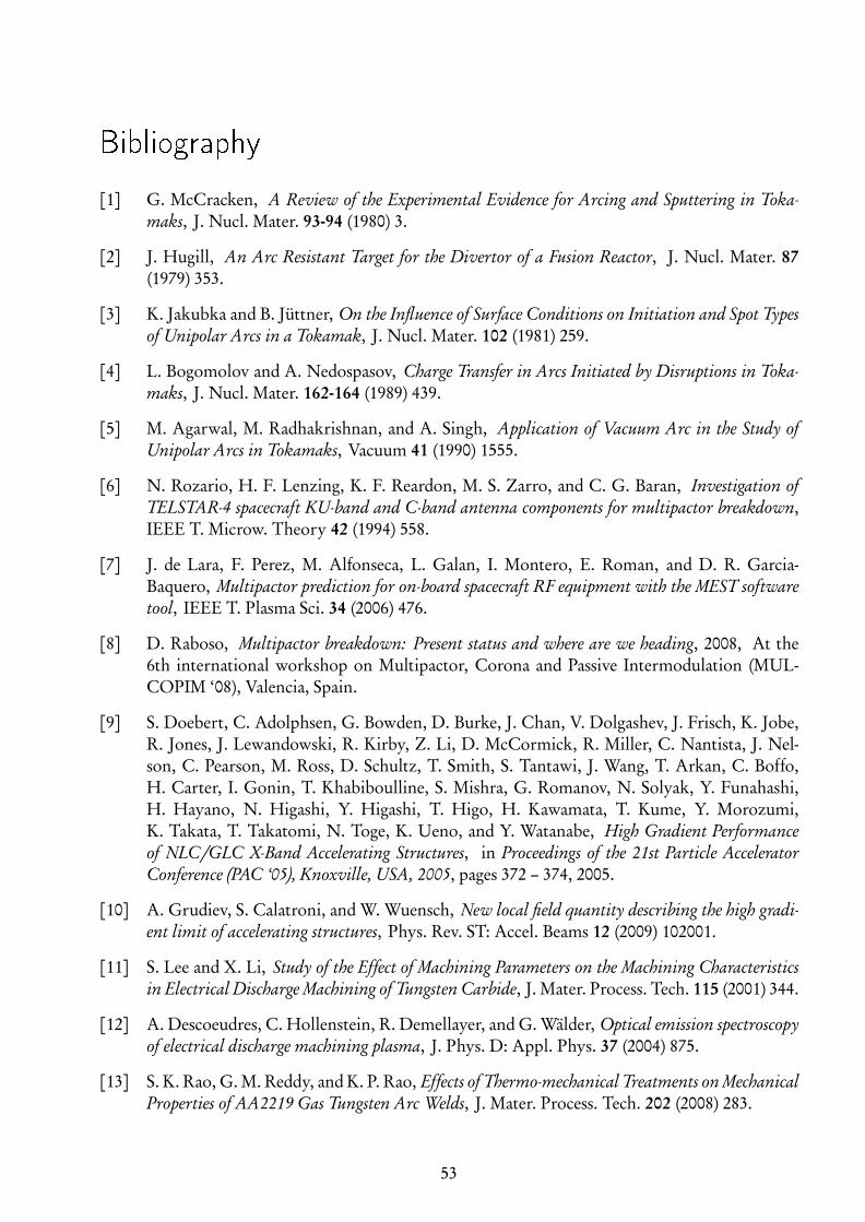
Bibliography

[1] G. McCracken, A Review of the Experimental Evidence for Arcing and Sputtering in Toka-maks, J. Nucl. Mater. 93-94 (1980) 3.

[2] J. Hugill, An Arc Resistant Target for the Divertor of a Fusion Reactor, J. Nucl. Mater. 87(1979) 353.

[3] K. Jakubka and B. Jüttner, On the Influence of Surface Conditions on Initiation and Spot Typesof Unipolar Arcs in a Tokamak, J. Nucl. Mater. 102 (1981) 259.

[4] L. Bogomolov and A. Nedospasov, Charge Transfer in Arcs Initiated by Disruptions in Toka-maks, J. Nucl. Mater. 162-164 (1989) 439.

[5] M. Agarwal, M. Radhakrishnan, and A. Singh, Application of Vacuum Arc in the Study ofUnipolar Arcs in Tokamaks, Vacuum 41 (1990) 1555.

[6] N. Rozario, H. F. Lenzing, K. F. Reardon, M. S. Zarro, and C. G. Baran, Investigation ofTELSTAR-4 spacecraft KU-band and C-band antenna components for multipactor breakdown,IEEE T. Microw. Theory 42 (1994) 558.

[7] J. de Lara, F. Perez, M. Alfonseca, L. Galan, I. Montero, E. Roman, and D. R. Garcia-Baquero, Multipactor prediction for on-board spacecraft RF equipment with the MEST softwaretool, IEEE T. Plasma Sci. 34 (2006) 476.

[8] D. Raboso, Multipactor breakdown: Present status and where are we heading, 2008, At the6th international workshop on Multipactor, Corona and Passive Intermodulation (MUL-COPIM ‘08), Valencia, Spain.

[9] S. Doebert, C. Adolphsen, G. Bowden, D. Burke, J. Chan, V. Dolgashev, J. Frisch, K. Jobe,R. Jones, J. Lewandowski, R. Kirby, Z. Li, D. McCormick, R. Miller, C. Nantista, J. Nel-son, C. Pearson, M. Ross, D. Schultz, T. Smith, S. Tantawi, J. Wang, T. Arkan, C. Boffo,H. Carter, I. Gonin, T. Khabiboulline, S. Mishra, G. Romanov, N. Solyak, Y. Funahashi,H. Hayano, N. Higashi, Y. Higashi, T. Higo, H. Kawamata, T. Kume, Y. Morozumi,K. Takata, T. Takatomi, N. Toge, K. Ueno, and Y. Watanabe, High Gradient Performanceof NLC/GLC X-Band Accelerating Structures, in Proceedings of the 21st Particle AcceleratorConference (PAC ‘05), Knoxville, USA, 2005, pages 372 – 374, 2005.

[10] A. Grudiev, S. Calatroni, and W. Wuensch, New local field quantity describing the high gradi-ent limit of accelerating structures, Phys. Rev. ST: Accel. Beams 12 (2009) 102001.

[11] S. Lee and X. Li, Study of the Effect of Machining Parameters on the Machining Characteristicsin Electrical Discharge Machining of Tungsten Carbide, J. Mater. Process. Tech. 115 (2001) 344.

[12] A. Descoeudres, C. Hollenstein, R. Demellayer, and G. Wälder, Optical emission spectroscopyof electrical discharge machining plasma, J. Phys. D: Appl. Phys. 37 (2004) 875.

[13] S. K. Rao, G. M. Reddy, and K. P. Rao, Effects of Thermo-mechanical Treatments on MechanicalProperties of AA2219 Gas Tungsten Arc Welds, J. Mater. Process. Tech. 202 (2008) 283.

53

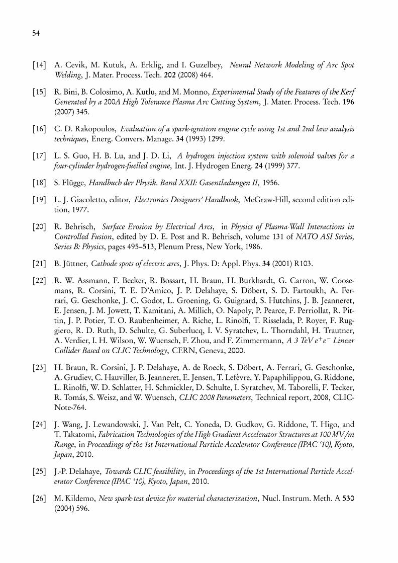
54

[14] A. Cevik, M. Kutuk, A. Erklig, and I. Guzelbey, Neural Network Modeling of Arc SpotWelding, J. Mater. Process. Tech. 202 (2008) 464.

[15] R. Bini, B. Colosimo, A. Kutlu, and M. Monno, Experimental Study of the Features of the KerfGenerated by a 200A High Tolerance Plasma Arc Cutting System, J. Mater. Process. Tech. 196(2007) 345.

[16] C. D. Rakopoulos, Evaluation of a spark-ignition engine cycle using 1st and 2nd law analysistechniques, Energ. Convers. Manage. 34 (1993) 1299.

[17] L. S. Guo, H. B. Lu, and J. D. Li, A hydrogen injection system with solenoid valves for afour-cylinder hydrogen-fuelled engine, Int. J. Hydrogen Energ. 24 (1999) 377.

[18] S. Flügge, Handbuch der Physik. Band XXII: Gasentladungen II, 1956.

[19] L. J. Giacoletto, editor, Electronics Designers’ Handbook, McGraw-Hill, second edition edi-tion, 1977.

[20] R. Behrisch, Surface Erosion by Electrical Arcs, in Physics of Plasma-Wall Interactions inControlled Fusion, edited by D. E. Post and R. Behrisch, volume 131 of NATO ASI Series,Series B: Physics, pages 495–513, Plenum Press, New York, 1986.

[21] B. Jüttner, Cathode spots of electric arcs, J. Phys. D: Appl. Phys. 34 (2001) R103.

[22] R. W. Assmann, F. Becker, R. Bossart, H. Braun, H. Burkhardt, G. Carron, W. Coose-mans, R. Corsini, T. E. D’Amico, J. P. Delahaye, S. Döbert, S. D. Fartoukh, A. Fer-rari, G. Geschonke, J. C. Godot, L. Groening, G. Guignard, S. Hutchins, J. B. Jeanneret,E. Jensen, J. M. Jowett, T. Kamitani, A. Millich, O. Napoly, P. Pearce, F. Perriollat, R. Pit-tin, J. P. Potier, T. O. Raubenheimer, A. Riche, L. Rinolfi, T. Risselada, P. Royer, F. Rug-giero, R. D. Ruth, D. Schulte, G. Suberlucq, I. V. Syratchev, L. Thorndahl, H. Trautner,A. Verdier, I. H. Wilson, W. Wuensch, F. Zhou, and F. Zimmermann, A 3 TeV e+e− LinearCollider Based on CLIC Technology, CERN, Geneva, 2000.

[23] H. Braun, R. Corsini, J. P. Delahaye, A. de Roeck, S. Döbert, A. Ferrari, G. Geschonke,A. Grudiev, C. Hauviller, B. Jeanneret, E. Jensen, T. Lefèvre, Y. Papaphilippou, G. Riddone,L. Rinolfi, W. D. Schlatter, H. Schmickler, D. Schulte, I. Syratchev, M. Taborelli, F. Tecker,R. Tomás, S. Weisz, and W. Wuensch, CLIC 2008 Parameters, Technical report, 2008, CLIC-Note-764.

[24] J. Wang, J. Lewandowski, J. Van Pelt, C. Yoneda, D. Gudkov, G. Riddone, T. Higo, andT. Takatomi, Fabrication Technologies of the High Gradient Accelerator Structures at 100 MV/mRange, in Proceedings of the 1st International Particle Accelerator Conference (IPAC ‘10), Kyoto,Japan, 2010.

[25] J.-P. Delahaye, Towards CLIC feasibility, in Proceedings of the 1st International Particle Accel-erator Conference (IPAC ‘10), Kyoto, Japan, 2010.

[26] M. Kildemo, New spark-test device for material characterization, Nucl. Instrum. Meth. A 530(2004) 596.

55

[27] M. Kildemo, S. Calatroni, and M. Taborelli, Breakdown and field emission conditioning ofCu, Mo, and W, Phys. Rev. ST: Accel. Beams 7 (2004) 092003.

[28] R. Latham, editor, High Voltage Vacuum Insulation – Basic Concepts and Technological Prac-tice, Academic Press, London, 1995.

[29] G. E. Vibrans, Field emission in vacuum voltage breakdown, Technical report 353, Lincolnlaboratory, MIT, Cambridge, Massachusetts, USA, 1964.

[30] D. W. Williams and W. T. Williams, Field-emitted current necessary for cathode-initiated vac-uum breakdown, J. Phys. D: Appl. Phys. 5 (1972) 280.

[31] P. Rossetti, F. Paganucci, and M. Andrenucci, Numerical model of thermoelectric phenomenaleading to cathode-spot ignition, IEEE T. Plasma Sci. 30 (2002) 1561.

[32] F. Djurabekova, S. Parviainen, A. Pohjonen, and K. Nordlund, Atomistic modeling of metalsurfaces under electric fields: Direct coupling of electric fields to a molecular dynamics algorithm,Phys. Rev. E 83 (2011) 026704.

[33] S. Parviainen, F. Djurabekova, H. Timko, and K. Nordlund, Electronic processes in moleculardynamics simulations of nanoscale metal tips under electric fields, Comp. Mater. Sci. 50 (2011)2075 .

[34] A. S. Pohjonen, F. Djurabekova, K. Nordlund, A. Kuronen, and S. P. Fitzgerald, Dislocationnucleation from near surface void under static tensile stress in Cu, J. Appl. Phys. 110 (2011)023509.

[35] S. Calatroni, A. Descoeudres, J. Kovermann, M. Taborelli, H. Timko, W. Wuensch,F. Djurabekova, K. Nordlund, A. Pohjonen, and A. Kuronen, Breakdown Studies for theCLIC Accelerating Structures, Technical Report EuCARD-CON-2011-005, 2010.

[36] A. Anders, Cathodic Arcs – From Fractal Spots to Energetic Condensation, Springer Sci-ence+Business Media, LLC, 2008.

[37] J. Wesson, Tokamaks, Clarendon Press, Oxford, second edition, 1997, Chap. 9.8, Arcing.

[38] B. Jüttner, Nanosecond displacement times of arc cathode spots in vacuum, IEEE T. Plasma Sci.27 (1999) 836.

[39] E. L. Murphy and R. H. Good, Thermionic Emission, Field Emission, and the TransitionRegion, Phys. Rev. 102 (1956) 1464.

[40] A. Descoeudres, T. Ramsvik, S. Calatroni, M. Taborelli, and W. Wuensch, dc breakdownconditioning and breakdown rate of metals and metallic alloys under ultrahigh vacuum, Phys.Rev. ST: Accel. Beams 12 (2009) 032001.

[41] A. Anders, S. Anders, B. Juttner, W. Botticher, H. Luck, and G. Schroder, Pulsed dye laserdiagnostics of vacuum arc cathode spots, IEEE T. Plasma Sci. 20 (1992) 466.

[42] N. Vogel and V. Skvortsov, Plasma parameters within the cathode spot of laser-induced vacuumarcs: experimental and theoretical investigations, IEEE T. Plasma Sci. 25 (1997) 553.

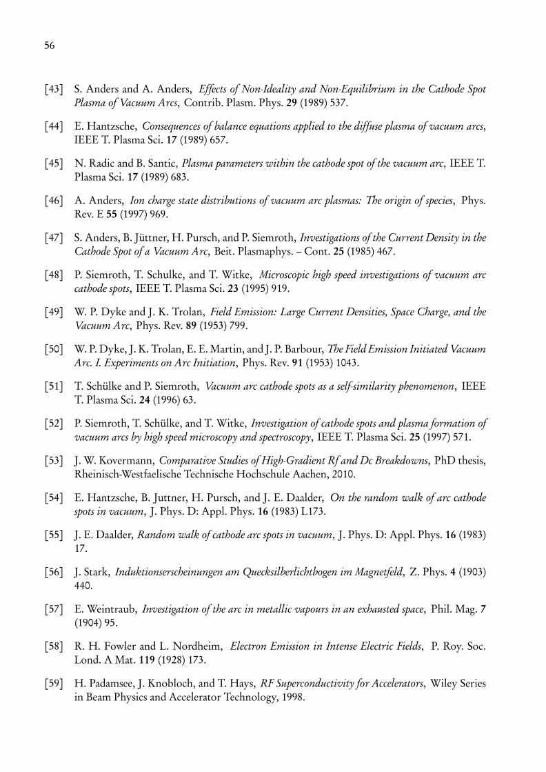
56

[43] S. Anders and A. Anders, Effects of Non-Ideality and Non-Equilibrium in the Cathode SpotPlasma of Vacuum Arcs, Contrib. Plasm. Phys. 29 (1989) 537.

[44] E. Hantzsche, Consequences of balance equations applied to the diffuse plasma of vacuum arcs,IEEE T. Plasma Sci. 17 (1989) 657.

[45] N. Radic and B. Santic, Plasma parameters within the cathode spot of the vacuum arc, IEEE T.Plasma Sci. 17 (1989) 683.

[46] A. Anders, Ion charge state distributions of vacuum arc plasmas: The origin of species, Phys.Rev. E 55 (1997) 969.

[47] S. Anders, B. Jüttner, H. Pursch, and P. Siemroth, Investigations of the Current Density in theCathode Spot of a Vacuum Arc, Beit. Plasmaphys. – Cont. 25 (1985) 467.

[48] P. Siemroth, T. Schulke, and T. Witke, Microscopic high speed investigations of vacuum arccathode spots, IEEE T. Plasma Sci. 23 (1995) 919.

[49] W. P. Dyke and J. K. Trolan, Field Emission: Large Current Densities, Space Charge, and theVacuum Arc, Phys. Rev. 89 (1953) 799.

[50] W. P. Dyke, J. K. Trolan, E. E. Martin, and J. P. Barbour, The Field Emission Initiated VacuumArc. I. Experiments on Arc Initiation, Phys. Rev. 91 (1953) 1043.

[51] T. Schülke and P. Siemroth, Vacuum arc cathode spots as a self-similarity phenomenon, IEEET. Plasma Sci. 24 (1996) 63.

[52] P. Siemroth, T. Schülke, and T. Witke, Investigation of cathode spots and plasma formation ofvacuum arcs by high speed microscopy and spectroscopy, IEEE T. Plasma Sci. 25 (1997) 571.

[53] J. W. Kovermann, Comparative Studies of High-Gradient Rf and Dc Breakdowns, PhD thesis,Rheinisch-Westfaelische Technische Hochschule Aachen, 2010.

[54] E. Hantzsche, B. Juttner, H. Pursch, and J. E. Daalder, On the random walk of arc cathodespots in vacuum, J. Phys. D: Appl. Phys. 16 (1983) L173.

[55] J. E. Daalder, Random walk of cathode arc spots in vacuum, J. Phys. D: Appl. Phys. 16 (1983)17.

[56] J. Stark, Induktionserscheinungen am Quecksilberlichtbogen im Magnetfeld, Z. Phys. 4 (1903)440.

[57] E. Weintraub, Investigation of the arc in metallic vapours in an exhausted space, Phil. Mag. 7(1904) 95.

[58] R. H. Fowler and L. Nordheim, Electron Emission in Intense Electric Fields, P. Roy. Soc.Lond. A Mat. 119 (1928) 173.

[59] H. Padamsee, J. Knobloch, and T. Hays, RF Superconductivity for Accelerators, Wiley Seriesin Beam Physics and Accelerator Technology, 1998.

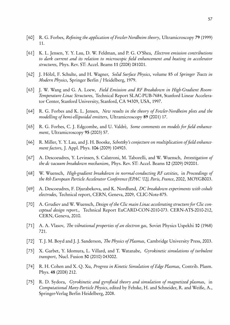
57

[60] R. G. Forbes, Refining the application of Fowler-Nordheim theory, Ultramicroscopy 79 (1999)11.

[61] K. L. Jensen, Y. Y. Lau, D. W. Feldman, and P. G. O’Shea, Electron emission contributionsto dark current and its relation to microscopic field enhancement and heating in acceleratorstructures, Phys. Rev. ST: Accel. Beams 11 (2008) 081001.

[62] J. Hölzl, F. Schulte, and H. Wagner, Solid Surface Physics, volume 85 of Springer Tracts inModern Physics, Springer Berlin /Heidelberg, 1979.

[63] J. W. Wang and G. A. Loew, Field Emission and RF Breakdown in High-Gradient Room-Temperature Linac Structures, Technical Report SLAC-PUB-7684, Stanford Linear Accelera-tor Center, Stanford University, Stanford, CA 94309, USA, 1997.

[64] R. G. Forbes and K. L. Jensen, New results in the theory of Fowler-Nordheim plots and themodelling of hemi-ellipsoidal emitters, Ultramicroscopy 89 (2001) 17.

[65] R. G. Forbes, C. J. Edgcombe, and U. Valdrè, Some comments on models for field enhance-ment, Ultramicroscopy 95 (2003) 57.

[66] R. Miller, Y. Y. Lau, and J. H. Booske, Schottky’s conjecture on multiplication of field enhance-ment factors, J. Appl. Phys. 106 (2009) 104903.

[67] A. Descoeudres, Y. Levinsen, S. Calatroni, M. Taborelli, and W. Wuensch, Investigation ofthe dc vacuum breakdown mechanism, Phys. Rev. ST: Accel. Beams 12 (2009) 092001.

[68] W. Wuensch, High-gradient breakdown in normal-conducting RF cavities, in Proceedings ofthe 8th European Particle Accelerator Conference (EPAC ‘02), Paris, France, 2002, MOYGB003.

[69] A. Descoeudres, F. Djurabekova, and K. Nordlund, DC breakdown experiments with cobaltelectrodes, Technical report, CERN, Geneva, 2009, CLIC-Note-875.

[70] A. Grudiev and W. Wuensch, Design of the Clic main Linac accelerating structure for Clic con-ceptual design report., Technical Report EuCARD-CON-2010-073. CERN-ATS-2010-212,CERN, Geneva, 2010.

[71] A. A. Vlasov, The vibrational properties of an electron gas, Soviet Physics Uspekhi 10 (1968)721.

[72] T. J. M. Boyd and J. J. Sanderson, The Physics of Plasmas, Cambridge University Press, 2003.

[73] X. Garbet, Y. Idomura, L. Villard, and T. Watanabe, Gyrokinetic simulations of turbulenttransport, Nucl. Fusion 50 (2010) 043002.

[74] R. H. Cohen and X. Q. Xu, Progress in Kinetic Simulation of Edge Plasmas, Contrib. Plasm.Phys. 48 (2008) 212.

[75] R. D. Sydora, Gyrokinetic and gyrofluid theory and simulation of magnetized plasmas, inComputational Many-Particle Physics, edited by Fehske, H. and Schneider, R. and Weiße, A.,Springer-Verlag Berlin Heidelberg, 2008.

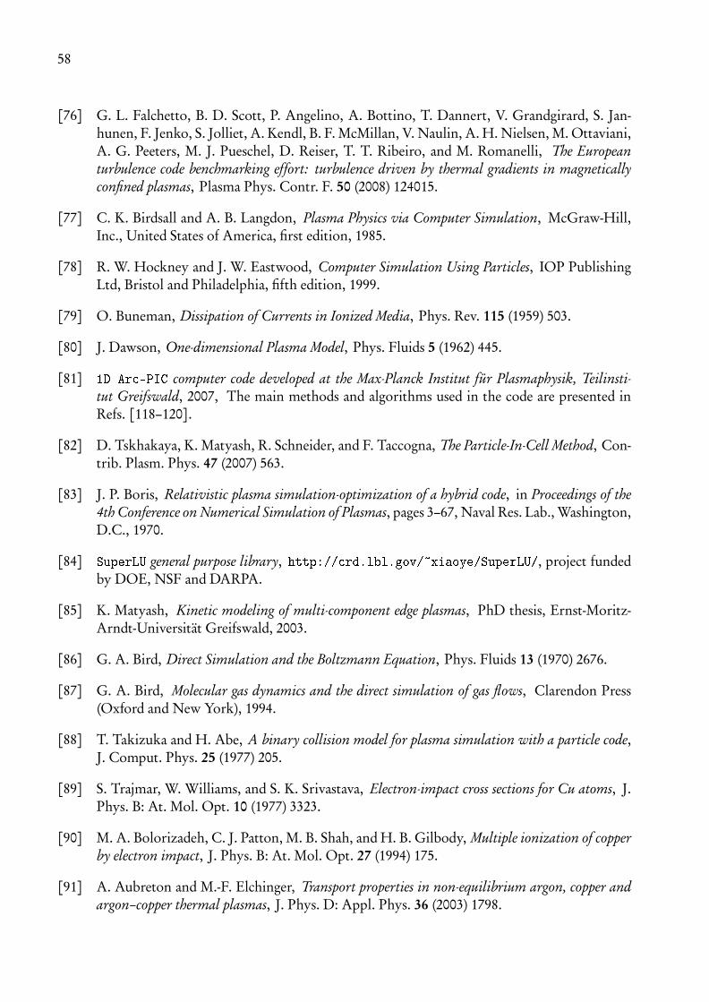
58

[76] G. L. Falchetto, B. D. Scott, P. Angelino, A. Bottino, T. Dannert, V. Grandgirard, S. Jan-hunen, F. Jenko, S. Jolliet, A. Kendl, B. F. McMillan, V. Naulin, A. H. Nielsen, M. Ottaviani,A. G. Peeters, M. J. Pueschel, D. Reiser, T. T. Ribeiro, and M. Romanelli, The Europeanturbulence code benchmarking effort: turbulence driven by thermal gradients in magneticallyconfined plasmas, Plasma Phys. Contr. F. 50 (2008) 124015.

[77] C. K. Birdsall and A. B. Langdon, Plasma Physics via Computer Simulation, McGraw-Hill,Inc., United States of America, first edition, 1985.

[78] R. W. Hockney and J. W. Eastwood, Computer Simulation Using Particles, IOP PublishingLtd, Bristol and Philadelphia, fifth edition, 1999.

[79] O. Buneman, Dissipation of Currents in Ionized Media, Phys. Rev. 115 (1959) 503.

[80] J. Dawson, One-dimensional Plasma Model, Phys. Fluids 5 (1962) 445.

[81] 1D Arc-PIC computer code developed at the Max-Planck Institut für Plasmaphysik, Teilinsti-tut Greifswald, 2007, The main methods and algorithms used in the code are presented inRefs. [118–120].

[82] D. Tskhakaya, K. Matyash, R. Schneider, and F. Taccogna, The Particle-In-Cell Method, Con-trib. Plasm. Phys. 47 (2007) 563.

[83] J. P. Boris, Relativistic plasma simulation-optimization of a hybrid code, in Proceedings of the4th Conference on Numerical Simulation of Plasmas, pages 3–67, Naval Res. Lab., Washington,D.C., 1970.

[84] SuperLU general purpose library, http://crd.lbl.gov/~xiaoye/SuperLU/, project fundedby DOE, NSF and DARPA.

[85] K. Matyash, Kinetic modeling of multi-component edge plasmas, PhD thesis, Ernst-Moritz-Arndt-Universität Greifswald, 2003.

[86] G. A. Bird, Direct Simulation and the Boltzmann Equation, Phys. Fluids 13 (1970) 2676.

[87] G. A. Bird, Molecular gas dynamics and the direct simulation of gas flows, Clarendon Press(Oxford and New York), 1994.

[88] T. Takizuka and H. Abe, A binary collision model for plasma simulation with a particle code,J. Comput. Phys. 25 (1977) 205.

[89] S. Trajmar, W. Williams, and S. K. Srivastava, Electron-impact cross sections for Cu atoms, J.Phys. B: At. Mol. Opt. 10 (1977) 3323.

[90] M. A. Bolorizadeh, C. J. Patton, M. B. Shah, and H. B. Gilbody, Multiple ionization of copperby electron impact, J. Phys. B: At. Mol. Opt. 27 (1994) 175.

[91] A. Aubreton and M.-F. Elchinger, Transport properties in non-equilibrium argon, copper andargon–copper thermal plasmas, J. Phys. D: Appl. Phys. 36 (2003) 1798.

59

[92] D. J. Larson, A Coulomb collision model for PIC plasma simulation, J. Comput. Phys. 188(2003) 123.

[93] V. Vahedi and M. Surendra, A Monte Carlo collision model for the particle-in-cell method:applications to argon and oxygen discharges, Comput. Phys. Commun. 87 (1995) 179.

[94] P. A. Chatterton, A theoretical study of field emission initiated vacuum breakdown, Proc.Phys. Soc. 88 (1966) 231.

[95] R. G. Forbes, Field evaporation theory: a review of basic ideas, Appl. Surf. Sci. 87-88 (1995)1, Proceedings of the 41st International Field Emission Symposium.

[96] Y. Yamamura and H. Tawara, Energy dependence of ion-induced sputtering yields frommonatomic solids at normal incidence, Atom. Data Nucl. Data 62 (1996) 149.

[97] B. Chapman, Glow Discharge Processes – Sputtering and Plasma Etching, John Wiley & Sons,1980.

[98] M. P. Allen and D. J. Tildesley, Computer simulation of liquids, Oxford University Press,1989.

[99] K. Nordlund, PARCAS computer code, 2011, The main methods and algorithms used in thecode are presented in Refs. [102] and [103].

[100] K. Nordlund, Molecular dynamics simulation of ion ranges in the 1-100 keV energy range,Comp. Mater. Sci. 3 (1995) 448.

[101] M. J. Sabochick and N. Q. Lam, Radiation-Induced Amorphization of Ordered IntermetallicCompounds CuTi, CuTi3, and Cu4Ti3 A molecular-dynamics study, Phys. Rev. B 43 (1991)5243.

[102] K. Nordlund, M. Ghaly, R. S. Averback, M. Caturla, T. Diaz de la Rubia, and J. Tarus, Defectproduction in collision cascades in elemental semiconductors and fcc metals, Phys. Rev. B 57(1998) 7556.

[103] M. Ghaly, K. Nordlund, and R. Averback, Molecular Dynamics Investigations of Surface Dam-age Produced by keV Self-Bombardment of Solids, Philos. Mag. A 79 (1999) 795.

[104] K. Nordlund, J. Keinonen, M. Ghaly, and R. S. Averback, Coherent displacement of atomsduring ion irradiation, Nature (London) 398 (1999) 49.

[105] M. Daw and M. Baskes, Semiempirical, Quantum Mechanical Calculation of Hydrogen Em-brittlement in Metals, Phys. Rev. Lett. 50 (1983) 1285.

[106] M. Daw and M. Baskes, Embedded-atom Method: Derivation and Application to Impurities,Surfaces and other Defects in Metals, Phys. Rev. B 29 (1984) 6443.

[107] P. Hohenberg and W. Kohn, Inhomogeneous Electron Gas, Phys. Rev. 136 (1964) B864.

[108] J. Samela and K. Nordlund, Atomistic Simulation of the Transition from Atomistic to Macro-scopic Cratering, Phys. Rev. Lett. 101 (2008) 027601.

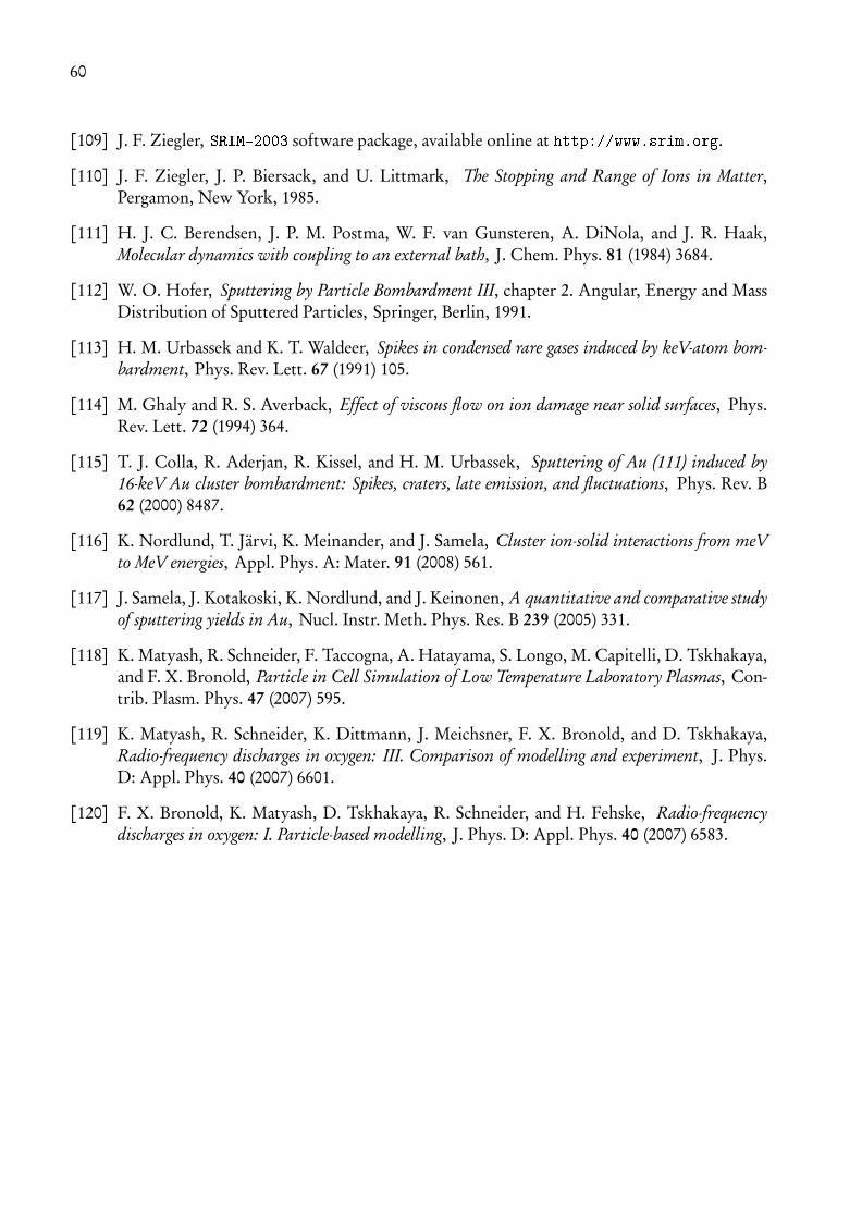
60

[109] J. F. Ziegler, SRIM-2003 software package, available online at http://www.srim.org.

[110] J. F. Ziegler, J. P. Biersack, and U. Littmark, The Stopping and Range of Ions in Matter,Pergamon, New York, 1985.

[111] H. J. C. Berendsen, J. P. M. Postma, W. F. van Gunsteren, A. DiNola, and J. R. Haak,Molecular dynamics with coupling to an external bath, J. Chem. Phys. 81 (1984) 3684.

[112] W. O. Hofer, Sputtering by Particle Bombardment III, chapter 2. Angular, Energy and MassDistribution of Sputtered Particles, Springer, Berlin, 1991.

[113] H. M. Urbassek and K. T. Waldeer, Spikes in condensed rare gases induced by keV-atom bom-bardment, Phys. Rev. Lett. 67 (1991) 105.

[114] M. Ghaly and R. S. Averback, Effect of viscous flow on ion damage near solid surfaces, Phys.Rev. Lett. 72 (1994) 364.

[115] T. J. Colla, R. Aderjan, R. Kissel, and H. M. Urbassek, Sputtering of Au (111) induced by16-keV Au cluster bombardment: Spikes, craters, late emission, and fluctuations, Phys. Rev. B62 (2000) 8487.

[116] K. Nordlund, T. Järvi, K. Meinander, and J. Samela, Cluster ion-solid interactions from meVto MeV energies, Appl. Phys. A: Mater. 91 (2008) 561.

[117] J. Samela, J. Kotakoski, K. Nordlund, and J. Keinonen, A quantitative and comparative studyof sputtering yields in Au, Nucl. Instr. Meth. Phys. Res. B 239 (2005) 331.

[118] K. Matyash, R. Schneider, F. Taccogna, A. Hatayama, S. Longo, M. Capitelli, D. Tskhakaya,and F. X. Bronold, Particle in Cell Simulation of Low Temperature Laboratory Plasmas, Con-trib. Plasm. Phys. 47 (2007) 595.

[119] K. Matyash, R. Schneider, K. Dittmann, J. Meichsner, F. X. Bronold, and D. Tskhakaya,Radio-frequency discharges in oxygen: III. Comparison of modelling and experiment, J. Phys.D: Appl. Phys. 40 (2007) 6601.

[120] F. X. Bronold, K. Matyash, D. Tskhakaya, R. Schneider, and H. Fehske, Radio-frequencydischarges in oxygen: I. Particle-based modelling, J. Phys. D: Appl. Phys. 40 (2007) 6583.