modelling volatility: arch, garch and other modelsstats.lse.ac.uk/q.yao/talks/archgarch.pdf ·...
TRANSCRIPT

Modelling Volatility: ARCH, GARCH and
Other Models
Qiwei Yao
London School of Economics
• ARCH & GARCH models: properties, estimation and tests
• A numerical example with S&P 500 index returns
• Other univariate volatility models
Reference: Fan & Yao (2003/5). Nonlinear Time Series. Springer:
§4.2.

Standard time series models: model conditional means
Volatility models: model conditional variances — (conditional) het-
eroscedasticity
Goal: Explain and model risk and uncertainty
Background: It is often found in finance that the larger values of
time series also lead to larger instability (ie. larger variances)

1. Yields of Treasury
Bills from July 17, 1959
to September 24, 1999
(source: Federal Reserve):
(a) Yields of three-month
Treasury Bills; (b) yields of
six-month Treasury Bills; (c)
yields of twelve-month Trea-
sury Bills.
It is clear that the yields
of Treasury Bills exhibit the
largest variation around the
peaks.
(a)
0 500 1000 1500 2000
510
15
Yields of 3-month Treasury bills
(b)
0 500 1000 1500 2000
24
68
1012
1416
Yields of 6-month Treasury bills
(c)
0 500 1000 1500 2000
46
810
1214
Yields of 12-month Treasury bills

2. Annual sunspot data
••••
•
•
•••••••••
•
•
••
••••••
•
•
•
•
•
•
•
••
•
•
••
••
•
•
••
•••
•
•
••
••
•
•••
•
•••
•
•
••
••
•
•
••
•
•
••
•
•
•
•
•
•
•
•
•
•
•
•
••
•
•
••
••
••••••
•••••
•
••••••••
•••
••••••••
•
•
•••
•
•
••
•
•
•
•
•
•
•
•
••
•
•
•
•
•
•••
•
•
••
•
•
••
•
•
••
•
••
•
•
•
••
•
•
•••••
•
••••
•
•
••••
•
•
••
•
•
••
••••
•
•
•••
••
•
••••
••
•
•
•
•
•
•••
•
•••
•
•
••••
•
•
••
•
•
•
•
••
•
•
•
••
•
•
•
••
•
•
••
•
•
•
••
••
•
•
•••
••
••
••
•
•
••
•
•
•
•
••
•
•
•
••
•
•
•
time
1700 1750 1800 1850 1900 1950 2000
050
100
150
Number of Sunspots

Basic properties of ARCH models
Xt = σtεt, and σ2t = c0 + b1X2t−1 + · · ·+ bpX
2t−p,
where c0 ≥ 0, bj ≥ 0 are constants, {εt} ∼ IID(0,1), and εt is indepen-
dent of {Xt−k, k ≥ 1} for all t.
Theorem. (Chen & An 1998, Giraitis, Kokoszka & Leipus 2000)
(i) The necessary and sufficient condition for the above model defining
a unique strictly stationary process {Xt, t = 0,±1,±2, · · · } with EX2t <
∞ is∑p
j=1 bj < 1. Further,
EXt = 0 and EX2t = c0/{1−
p∑
j=1
bj},
and Xt ≡ 0 for all t if c0 = 0.
(ii) If Eε4t < ∞ and max{1, (Eε4t )1/2}∑p
j=1 bj < 1, the strictly station-
ary solution has the finite fourth moment, namely EX4t < ∞.

Remark. (i) Stationary ARCH process {Xt} is WN(0, c0/(1−∑p
j=1 bj)).
(ii) It follows from the model that
X2t = c0 + b1X
2t−1 + · · ·+ bpX
2t−p + et,
where
et = (ε2t − 1){c0 +p∑
j=1
bjX2t−p}.
Further,
E(et|Xt−k, Xt−k−1, · · · ) = 0, for any k ≥ 1.
Hence for any k > p,
Var(Xt+k|Xt−m, m ≥ 0) = c0 +
p∑
j=1
bjVar(Xt+k−j|Xt−m, m ≥ 0),
which reflects ‘volatility cluster’ in financial time series analysis.
(iii) Under the additional condition max{1, (Eε4t )1/2}∑p
j=1 bj < 1,

{et} ∼ WN(0, σ2e ) with
σ2e = Var(ε2t )E{c0 +p∑
j=1
bjX2t−p}2 < ∞.
Note that the condition∑p
j=1 bj < 1 implies that 1 − ∑pj=1 bjz
j 6= 0
for all |z| ≥ 1. Hence {X2t } is a causal AR(p) process. Therefore,
the ACF (also ACVF) of the process {X2t } can be easily calculated
in terms of its MA(∞)-representation, which implies the fact that for
all τ
Corr(X2t , X
2t+τ) > 0,
although Corr(Xt, Xt+τ) = 0.
(iv) The stationary ARCH process {Xt} has heavier tails than those
of the white noise {εt} based on which {Xt} is defined.

Let κε = E(ε4t )/(Eε2t )2 the kurtosis of the distribution of εt. Then
E(X4t |Xt−1, · · · , Xt−p) = σ4t Eε4t = κεσ
4t (Eε2t )
2
= κε{E(X2t |Xt−1, · · · , Xt−p)}2.
Now it follows from Jensen’s inequality that
E(X4t ) = κεE{E(X2
t |Xt−1, · · · , Xt−p)}2 ≥ κε(EX2t )
2.
Hence κx ≡ E(X4t )/(EX2
t )2 ≥ κε. In the case that εt is normal and
κx > κε = 3, Xt has leptokurtosis (i.e. fat tails).

Example. ARCH(1) model:
Xt = σtεt, and σ2t = c0 + b1X2t−1,
where {εt} ∼ IID(0,1), c0 > 0 and b1 ∈ (0,1). Then EX2t = c0/(1−b1),
and for k ≥ 1,
Var(Xt+k|Xt−j, j ≥ 0) = Var(Xt+k|Xt)
= c0 + b1Var(Xt+k−1|Xt) =c0(1− bk1)
1− b1+ bk1X
2t ,
which indicates that a large value of |Xt| will lead to large predictive
risk (i.e. conditional variance) in a sustained period in the immediate
future.
Suppose εt ∼ N(0,1). Under the condition 3b21 < 1, Corr(X2t , X
2t+τ) =
b|τ |1 , and {X2
t } follows a causal AR(1) equation
X2t = c0 + b1X
2t−1 + et,

where et = (ε2t − 1)(c0 + b1X2t−1). Hence,
EX4t = Eσ4t Eε4t = 3Eσ4t
= 3(c20 +2c0b1EX2t + b21EX4
t )
= 3(1− b1)2(EX2
t )2 +6(1− b1)b1(EX2
t )2 +3b21EX4
t
= 3(1− b21)(EX2t )
2 +3b21EX4t .
The last equality uses the fact that c0 = (1− b1)EX2t . Hence
EX4t
(EX2t )
2=
3(1− b21)
(1− 3b21)> 3.
Hence Xt has leptokurtosis (fat tails).

A sample of 1000
were generated from
the ARCH(1) model:
c0 = 1.5, b1 = 0.9,
and εt ∼ N(0,1)
•
•
•••••
•••••
••
••
••••
•
•
••
•
••
••••••••
•
•
•
•
••••••
••••
•
••••
•••••••••••
•
•
••••••
•
•••
••
••
•••••••
•
•
•••
•
•••••••••
••
•••
•
••••••••
•
•
•
•
•
•
•
•
•••
•••
•
••••
•
•
••
•••••••••••
••••••••
••
••••••
•
•
••
•
•
••••
•
•
••
••••
•
•
•
•
•
•••
•
•
••
•
••
•
•••
••
•
••
•
••••
•
•
••
•••••••••
••
••
••••
•••
••••
•
•
•••
•
•
•
(a) ARCH(1) time series
t0 50 100 150 200 250
-10
-50
510
-15 -10 -5 0 5 10 15
0.0
0.05
0.10
0.15
0.20
0.25
(b) Histogram
•
•
•
••••••••••
••••••••
•
•••
•
•••••••••••
••
•••••••
•
••
•
•
••••
•••
•
••••••••••••••
••
••
•
••
••
•••••••
•
•
•••••••••••
••••
••
•
•••••••••
•
••
•
••
•
••••
•
•••••••
•
•
•
•
•••••••••••••••••••
••
••••••
••
••
•
•
••••••••••••••
•
••••
•
•
•••••••••••••••
•
•••••
•
••••••••••••
•
•
•
•••••
•
•
••••••
•••
•
•
(c) Conditional STD
t0 50 100 150 200 250
24
68
•
•
•••• •
• ••• •
• •••
• •••
•
•••
•
••
••
••••• •
•
•
•
•••• •
••
• •••
•
••••
•• ••
• •• •••••
••••••
•
••
• •
• •••
•••••••
•
•
• •••
•••••••
••
••• •
••
••••• • ••
•
•
•
•
•
•
•
•• ••
•••
••
• ••
•
•
••
••• •••
•••••
• •••• •
• •••
••
•• •••
•
••
••
•• ••
•
•
••• •
••
••
•
•
••
••
•
•••
•••
•
•••
• •
•••
•••
••
•
•
••• •••
•• •• •
••
••
•••
••
••
• ••••
••
• ••
•
•••
•
••••
•••
••
••
• •• ••
•••
••
••
•• •
• ••
• ••
•
••
••
• ••
• ••
••
••••
••
•
••
• •••
• ••
••
••••
•
•
•
•
•
•••
•••
•
••• • •
• • •
•
•
••
•
• ••• ••
••
•
••
••
•••
• ••
•• •••
•• •
•
•••
••
•• ••• •
••
••
•••
•
••
•
•
•
•
•
•
•
• •
• ••
••• ••••
••
•
•
•••••••
• •••••••
•
•
• •
•
•
•• • •
••
•••••
••••
••
•
•••
•
••
••• ••• • • •
••
•
•
•
••••
•
••
•
•••••
•
••
••
•
•
• ••••
•
•••
• ••
• •• •• ••
•••
••••••
••• • • ••••
•• • •••
••
••
•••••
•• •
••
•
•
•
•
•• •
••
••
•• ••• •
•••
•
•
•
•
•
•
••
•
• ••
•
•• •
•••••
••••
• •
•
•
••
•
•
•
•
•••
••••
• ••
••
• •• •••••
• •••
•
••• •••
• ••••
• ••
••
• •• •
•
• ••• • •
••
••
•••
••
• ••
•••
••
•
•
••••••
•• ••
••••
••
•••
•••••
•
•
••••• ••••• •
•
•
•••
•
•
•• •
••
•• • ••
••• • ••• •••
•••
••• •••
• • •••
•
•
•
••
•••
•
••
••
••
••
••
••
••
••
•
••
•• •••
•••••
••
••
••• •• •
• ••
•••••
••
••
•
•••
•••••
•••
••
•
•
•• ••••
••
•
••
•
••
•
••
• ••••
••
•
•
•
•
•• •
•
•••
• •• •
••••
•••• ••
• •
•
•••
••••••
••• ••
••• •••
•• •
•
•
•
•• ••
•••
•• •
•
•
••
••• • ••
• •
•••
••
•
•
• ••
•••
•
•••
••• • •• ••
••••• • •••
•••• •
•
••
•
•
•
•
••
•
•
•••
••
•
•
•• ••••
(d) QQ-plot
Normal quantile
AR
CH
qua
ntile
-2 0 2
-15
-10
-50
510
15
Lag
AC
F
0 5 10 15 20 25 30
0.0
0.2
0.4
0.6
0.8
1.0
(e) ACF
Lag
AC
F
0 5 10 15 20 25 30
0.0
0.2
0.4
0.6
0.8
1.0
(f) ACF of squared series

A sample of 1000
were generated from
the ARCH(1) model:
c0 = 1.5, b1 = 0.4,
and εt ∼ N(0,1)
•
•
•••••
•••
••
••
•
•
•
•••
•
•
••
•
•
•
•
•
•
••••
•
•
•
•
•
••••
•
•
•
••
•
•
•••
•
•••
•
•
•
•••••
•
•
•••
••
•
•
•
••
••
••
•••
•
••
•
•
•
•••
•
••
•
•
••
•
••
••
••
•
•
••••••••
•
•
•
•
•
•
•
•
••
•
•
••
•
•
•••
•
•
•
•
••
•
•••
••
••
•
••
•••
•
••
••
•
•
••••
•
•
•
•
•
•
•••
•
•
•
••
••
•
•
•
•
•
•
•
•
•
•
•
•
••
•
••
•
•
•
•
••
•
••
•
••
••
•
•
••
••••
•
•
•••
••
•
•
•
•
•
•
•
••
••••
•
•
•
••
•
•
•
(a) ARCH(1) time series
t0 50 100 150 200 250
-4-2
02
4
-6 -4 -2 0 2 4
0.0
0.1
0.2
0.3
(b) Histogram
•
•
•
••••••••
••
••
•
•
•
•••
•
•••
•
•
••
•••••••
•
•
•
•••••••
•
••
••
•••
•
•••
•
•••••••
•••••
•
•
•
•
•
•
•
••
••
•••••••
•
•
•••
•
•••••••
••••
••
•
•
•••••••
•
•
•
•
•••
•
•••
•
•
••
•••••
•
•
•
•
••
•
•••••••••
•••••••
••
•
•
••••
••
••
•
•
••••
••••••••
•
•
•
••••
••
•••
•
••
••
•••••••
•
••••
•
•
••••••••
••••
•
•
•
•
•
•
••
••
••••••
•
••
•
•
(c) Conditional STD
t0 50 100 150 200 250
1.0
1.5
2.0
2.5
3.0
•
•
••••
•
•••
• •
••
•
•
•
•••
•
•
••
•
•
•
•
•
•
••••
•
•
•
•
•
•••
•
•
•
•
••
•
•
•••
•
•• •
•
••
•••
••
•
•
••
•
••
•
•
•
••
••
••
•••
•
••
•
•
•
• ••
•
••
••
••
•
••
••
••
•
•
•••• • •
••
•
•
•
•
•
•
•
•
• ••
•
••
•
•
• ••
•
•
•
•
••
•
••
••
••
•
••
•••
•
• •
••
•
•
• • ••
•
•
•
•
•
•
••
•
•
•
•
••
• •
•
•
•
•
•
•
•
•
•
•
•
•
••
•
••
•
•
•
•
• •
•
••
•
••
••
•
•
••
••••
•
•
•• •
••
•
•
•
•
•
•
•
• •
••••
•
•
•
••
•
•
••
•
•
•••
•
••
•
•
•
•
•
••
••
•
•
••
•
•
•
•
•
••
• •
•
••
•
•
••
•
•
••
•
• •
•
••
•
•
••
••
•
•
•
••••
••
•
•
•
••
• •
•
•
•
•
•
••
•
•••
•
••••
••
• •
•
•
•
••
•
•••
•
••
•
•
•
• •
•
•
••
•
••
•
•
••••
•
••
•
•
••
•
•
••••
••
•
•
•
•
••
•
•
•
•
•
•
•
•
•
•
•
••
•
•
•
• ••
•••
•
••
•
•
•••
••
•
•
•
••
••••
•
•
•
••
•
•
•
•• •
•
•
•
••••
••
••
••
•
•
••
•
•
•
• •
••••
• • •
•
•
•
•
•
•
•••
•
••
•
•••
••
•
••
•
•
•
•
••
••
•
•
••
•
••
•
••
• ••
•
•
•
••
•••
••
•
•
••
•• •
••••
••
•••
•
•
•
•
••• •
•
•
••
•
•
•
•
•
•
•
••
••
•••
•
••
• ••
••
•
•
•
•
•
•
•
•
•
•
•
•
•
•••
••
•••
••
•••
••
•
•
•
•
•
•
•
•
• ••
••••
••
•
•
••
••
••••
•
• •••
•
•••
••
•
••
••
•
•
•
•
•
•
•
•
••
•
•
•
•••
•
•
•
•
•
•
••
•
•
••
••
••
••
•
•
•
•••• •
•
• ••
••
•
•
••
••
•
••
•
••
•
•
• •• ••
••
••••
•
•
•••
•
•
••
•
•
•
••
••
•
•
•••
••
••
••
•
•
•
•••••
•
••
••
•
•
•
•
•
••
••
•
•
•
•
•
••
•
••
•
•
•
•
•
•
•
•
•
••
•
•
•
•
•
••••
•
•
•
•
•
•••
•
•
••
••
•••
•
••
••
•
••
••••
••
•
••
•
•
•
•
••
••
••
•
••
•
•
•
•
•
•
••
••
••
•
•
•
•
•
•
•
•
•
•
•
•
••
••
••
•
•••
•
•••••
••
•
••
••
•
••••
••
••
•
•••
••
•
••
•
•
•
•
•
••••
••
•
•
••
•
•
•
•
••••
•
•
• •
••
•
••
•
•
••
•
•
••
•
•
••
••
•
••
••
•
••
••
••
••
•
•
• •
••
•
•
•
•
•
•
•
•••
•• ••
•
•
•
•
•
••••
•
(d) QQ-plot
Normal quantile
AR
CH
qua
ntile
-2 0 2
-4-2
02
4
Lag
AC
F
0 5 10 15 20 25 30
0.0
0.2
0.4
0.6
0.8
1.0
(e) ACF
Lag
AC
F
0 5 10 15 20 25 30
0.0
0.2
0.4
0.6
0.8
1.0
(f) ACF of squared series

(a) and (c) the time plots of the first 250 X ′ts and σ′
ts; (b) the normalized histogram,
and the normal density function with the same mean and variance; (d) the sample
quantiles are plotted against the quantiles of N(0,1); (e) and (f) the sample ACFs
of {Xt} and {X2t } respectively.
(i) Large values of |Xt| leads to large σt.
(ii) {Xt} ∼ WN.
(iii) Heavy tails: heavier for larger b1.
(iv) ρ(k) ≈ ρ(k) for b1 = 0.4 but not for b1 = 0.9.

Basic properties of GARCH processes
Extension of ARCH:
dictated by economic insight, or
broadly statistical ideas.
Most important extension: generalized ARCH (GARCH) due to Boller-
slev (1986) and Taylor (1986).
ARCH(p) is useful only with large p in practice. GARCH provides a
parsimonious representation for complex auto-dependence structure.
GARCH(1,1): a widely used benchmark model.

GARCH(p,q): Xt = σtεt, σ2t = c0 +∑p
i=1 biX2t−i +
∑qj=1 ajσ
2t−j,
where c0 ≥ 0, bj ≥ 0 and aj ≥ 0 , {εt} ∼ IID(0,1), and εt is independent
of {Xt−k, k ≥ 1} for all t.
Let
et = X2t − σ2t = (ε2t − 1)(c0 +
p∑
i=1
biX2t−i +
q∑
j=1
ajσ2t−j).
Then
X2t = c0 +
p∑
i=1
biX2t−i +
q∑
j=1
ajσ2t−j + et
= c0 +p∨q∑
i=1
(bi + ai)X2t−i + et −
q∑
j=1
ajet−j,
where bp+j = aq+j = 0 for j ≥ 1. Thus {X2t } follows an ARMA
equation.
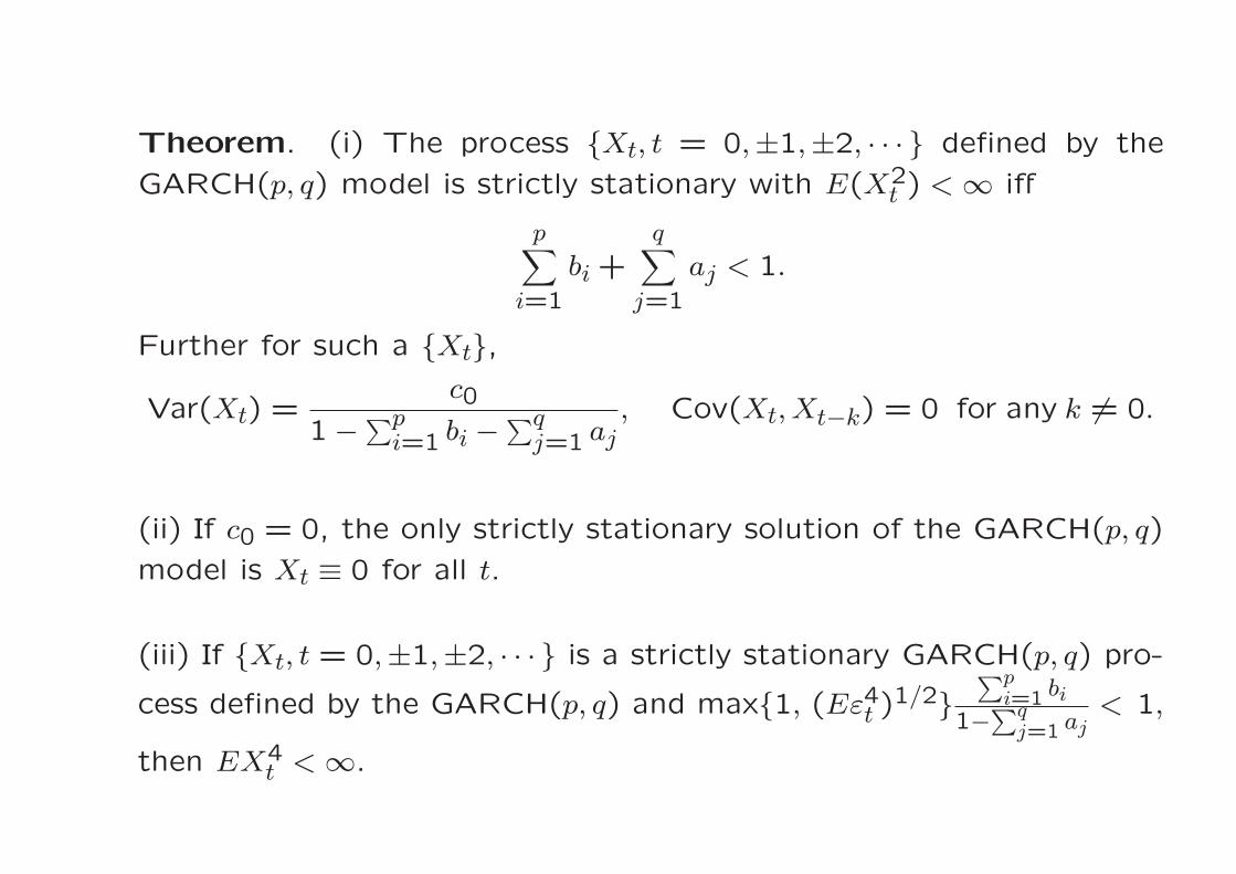
Theorem. (i) The process {Xt, t = 0,±1,±2, · · · } defined by the
GARCH(p, q) model is strictly stationary with E(X2t ) < ∞ iff
p∑
i=1
bi +q∑
j=1
aj < 1.
Further for such a {Xt},
Var(Xt) =c0
1− ∑pi=1 bi −
∑qj=1 aj
, Cov(Xt, Xt−k) = 0 for any k 6= 0.
(ii) If c0 = 0, the only strictly stationary solution of the GARCH(p, q)
model is Xt ≡ 0 for all t.
(iii) If {Xt, t = 0,±1,±2, · · · } is a strictly stationary GARCH(p, q) pro-
cess defined by the GARCH(p, q) and max{1, (Eε4t )1/2}
∑pi=1 bi
1−∑q
j=1 aj< 1,
then EX4t < ∞.

Note. Bougerol and Picard (1992) established a necessary and suf-
ficient condition for the existence of a strictly stationary solution of
the GARCH model, which may not have finite second moment. The
condition is defined in terms of Lyapunov exponents for some random
matrices associated with the model and is typically difficult to check
in practice.

Remark. (i) Stationary GARCH process is WN(0, c0(1 − ∑pi=1 bi −∑q
j=1 aj)).
(ii) The ARMA representation for X2t
X2t = c0 +
p∨q∑
i=1
(bi + ai)X2t−i + et −
q∑
j=1
ajet−j
is causal and invertible, where et = X2t − σ2t . Thus
(a) Formally {X2t } ∼ AR(∞)
(b) EX2t = Eε2t Eσ2t = Eσ2t , and E(Xt|Xt−1, Xt−2, · · · ) = 0.
(c) Eet = E(et|Xt−1, Xt−2, · · · ) = 0
(d) Var(Xt|Xt−1, Xt−2, · · · ) = E(X2t |Xt−1, Xt−2, · · · )
= c0 +∑p
i=1 biX2t−i +
∑qj=1 ajσ
2t−j = σ2t .
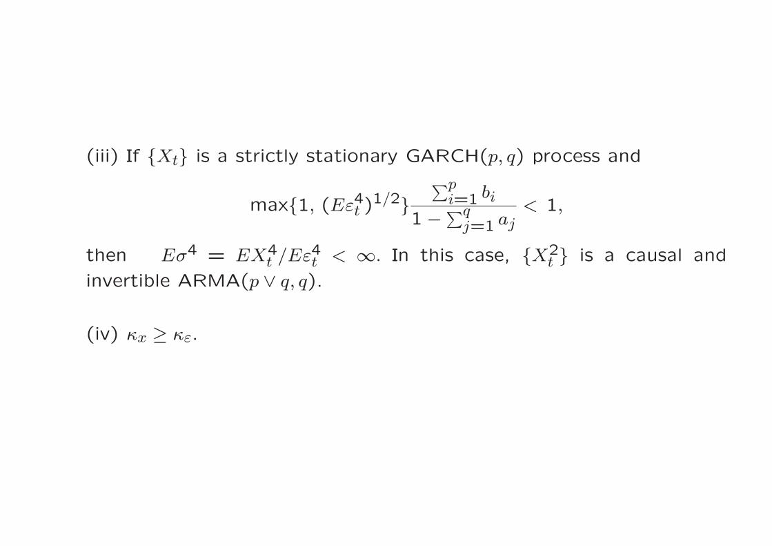
(iii) If {Xt} is a strictly stationary GARCH(p, q) process and
max{1, (Eε4t )1/2}
∑pi=1 bi
1− ∑qj=1 aj
< 1,
then Eσ4 = EX4t /Eε4t < ∞. In this case, {X2
t } is a causal and
invertible ARMA(p ∨ q, q).
(iv) κx ≥ κε.

Example. GARCH(1,1) model: Xt = σtεt and
σ2t = c0 + b1X2t−1 + a1σ
2t−1,
where c0, b1 and a1 are positive, b1 + a1 < 1, and {εt} ∼ IID(0,1).
Then EX2t = c0/(1− b1 − a1). Note
(1− a1B)σ2t = c0 + b1X2t−1.
Thus
σ2t =∞∑
j=0
aj1B
j(c0 + b1X2t−1) =
c01− a1
+ b1
∞∑
j=0
aj1X
2t−j−1.
and
Var(Xt|Xt−k, k ≥ 1) =c0
1− a1+ b1
∞∑
j=0
aj1X
2t−j−1,
which is a marked difference from ARCH(1) process for which
Var(Xt|Xt−k, k ≥ 1) depends on Xt−1 only: volatility cluster is more
persistent in GARCHprocesses than in ARCHprocesses.

Nelson (1990) showed that the necessary and sufficient condition for
existence of a strictly stationary GARCH(1,1) process is
E{log(b1ε2t + a1)} < 0.
By Jensen’s inequality,
E{log(b1ε2t + a1)} ≤ logE(b1ε2t + a1) = log(b1 + a1).
Hence, the condition b1 + a1 < 1 is sufficient for the existence of a
strictly (also weakly) stationary solution. If εt is normal, and
1.732b1 < 1− a1,
EX4t < ∞. Then {X2
t } is a causal and invertible ARMA(1,1) process
X2t = c0 + (b1 + a1)X
2t−1 + et − a1et−1,
where
et = (ε2t − 1)(c0 + b1X2t−1 + a1σ
2t−1).
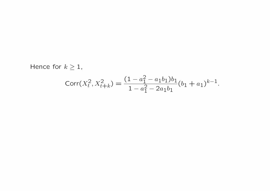
Hence for k ≥ 1,
Corr(X2t , X
2t+k) =
(1− a21 − a1b1)b1
1− a21 − 2a1b1(b1 + a1)
k−1.

A sample of 1000
were generated from
the GARCH(1,1)
model: c0 = 1.5,
b1 = 0.6, a1 = 0.3,
and εt ∼ N(0,1)
•
•••
••
•••
•
••••
•
•
•••••••••••
••
•
•
••
••
•••
••••
•
••••
•
•
••
•
•
•••
•
••••••••••••
••••
•
••
•••
•••
••
••
••
••
••
•
•••
••
••••
•
•
•
•
•
••
••
•••
•
•
••
•••
•
•
•
•
••
•
•••
•
••••••
•••
•
•
••
•
•••••••••
••
•
•
••
•••
•
••••••••
•
•••••
••••••
•
••
•
•••
•
••
•
•
•
•
•
•
•
••
•
•
•
•••••••
••
•
•
••••••••••
••••••
•
••
•
•
••••••
•••••
(a) GARCH(1,1) time series
t0 50 100 150 200 250
-15
-10
-50
510
15
-15 -10 -5 0 5 10 15
0.0
0.05
0.10
0.15
(b) Histogram
••••••••••••••••
•
••••••••••••
•
••
•••••
••
•••••••••
•
•••
••
•••
••••••••••••
••••
•
•••
•••
•••••••••••••
•
•••
••
••••
••
•
•
•
•
•
•••••••••
••
•
•
•
•
•••
•
•
••••••••••••
•
•••
••••••••••••
••
••
•••••••••••••••••
•
•••••••••••••
•
•••
•
•
•
•
•
•
••
••••••••••••••
•••••••••••••••
•••••
•••••••••••
(c) Conditional STD
t0 50 100 150 200 250
24
68
1012
•
••
•
• •
•••
•
••••
•
•
•••
••••
••• •
••
•
•
••
••
•• •
••••
•
••
• •
•
•
••
•
•
•••
•
•••
••
••
••••
•
•••
•
•
••
••
•
• ••
• •
••
• •
••
••
•
• ••
••
•••
•
•
•
•
•
•
••
••
••
•
•
•
••
•••
•
•
•
•
••
•
••
•
••••
••
• ••
•
•
••
•
•••
••
••
••
• •
•
•
••
•• •
•
•••••
••
•
•
•••
••
••••
• •
•
••
•
••
•
•
••
•
•
•
•
•
•
•
••
•
•
•
••• •••
•
••
•
•
•••
••
••
•••
••••
••
•
••
•
•
••
•••
•
•••••
••••
••
•
••
•
•
••
•••
••• • ••
••
•
•
•
•
•••
•
••
•
••••
•
•
••
•
•
•
•
•••
•
•
•
•••
•••
• •• •••
•
•••
•••••
•
•
•• •
• ••••
•
• • •••
••
•
•••••
•
••
•
•
•
•
•
•
•
•
••
•
•
•••
•• •• • •
••
•
•
•
•
•
•
•
•
•
•
•••
•
• ••
••
•••
• ••••
• •
•
•
• •
•
•
•
•
• ••
••••
••
•
•
••
•• •••••
••••
•
••• ••
•
• ••••
••
••
••
•
• ••
•
•
• • • ••
•
••
•••
••
• ••
•••
••
•
•
••••••
•• ••
••••
••
••
•
•••
••
•
•
• •••• ••
•••••
•
•• •
•
•
•••
•
•
••
••
•
••• •
•••
••••
••
•• • •••
• •••
•
•
•
•
••
•••
•
••
•
•
••
••
••
•
•
•
•
••
•
••
••
••
••
•••••
••
•
••• ••
•
• ••
•••••
••
••
•
•••
•••••
•••
•
•
•
•
••
••••
••
•
•
•
•
•
•
•
••
• ••
••
••
•
•
•
•
•
•
•
•
•
•
•
• •
••
•
•••
•
••• ••••
•
••
••
•••••••
• ••
••••
••
•••
•
•
•
•
••••
•••
•
• •
•
•
•
•
•••
• •
•
• •
••
•
••
•
•
••
•
•
••
•
•
••
•••
• ••
••
••••
• • ••
•
•
• ••
••
••
•
•
•
•
••
•
•
•••
•
•
•
•
•
•••••••
•••
••
•
••
•
••
•• ••
••
•
• •• ••
•• ••
••
•
••
••
•••
•• ••
•
••
• •
•
•••
•
•
••
•
••••
••
• ••
••••
• •••
••
•••
•
•
•
••
••
• •• •••
•••••
••
•
•••
•
••••
•
••••
••
••
••••
•• •
••
•
•
••••
••
• •
•••••
•
•
•
•
••••
••
••
•
•
•••••
•• •
•••
•
•••••
•••
••
• •••
•
•••• ••
••
• •• •
• ••
•
(d) QQ-plot
Normal quantile
GA
RC
H q
uant
ile
-2 0 2
-15
-10
-50
510
15
Lag
AC
F
0 5 10 15 20 25 30
0.0
0.2
0.4
0.6
0.8
1.0
(e) ACF
Lag
AC
F
0 5 10 15 20 25 30
0.0
0.2
0.4
0.6
0.8
1.0
(f) ACF of squared series

A sample of 1000
were generated from
the GARCH(1,1)
model: c0 = 1.5,
b1 = 0.3, a1 = 0.3,
and εt ∼ N(0,1)
•
•
•
•
••
•
••
•
••
••
•
•
••
•
•••
•
•
•••
••
•
•
•
•
•
•
•
••
••••
•
•
•
••
•
•
••
•
•
•••
•
••
•
•
•
•
•
•
••
•
•
•
••
•
•
•
•
•
•
•
••
•
••
•
•
••
•
•
•
•
•
••
•
••
•
•••
•
•
•
•
•
••
••
••
•
•
•
•
•
••
•
•
•
•
•
••
•
•••
•
•••
•
••
••
•
•
•
••
•
•••
•
•
•
•
•
•
••
•
•
••
•
••
•
•
••••
•
•
•
•
•
••
•
•
••
••
••
•
•
•
•
••
•
•
•
•
•
•
•
•
•
•
•
••
•
•
•
••
•••
•
•
••
•
•
•••
••
•
•
•
••
•••
•
•
•
•
•
•
•
•
•
•••
•
•
•
••••
(a) GARCH(1,1) time series
t0 50 100 150 200 250
-6-4
-20
24
-6 -4 -2 0 2 4
0.0
0.05
0.15
0.25
(b) Histogram
•
•••••••••
•
•••••
•
•
•••••••
••••
•
•
•
••
•••
••
••••••
•••
•
•••
•
•
•••
•
•••••••••••
•
•••
•
•••
•
••
••
•
•••
•••
••
••
•
•
••
••
•
•
••
••
••
•
••••••
•
••••
••
•
•
•
•
•••
•
•
••
••••••••••
•
•••
•
••••••••
•
••
•
•
••
•
•
•
••
•••••••
•
••••
•
••••••
•
••
••••
•
•
••
•
•
•
••
•
•
•
•••••••••
•
••••
•••••••
•
••••••
•
••
•••
•
•
••••
•••••
(c) Conditional STD
t0 50 100 150 200 250
1.5
2.0
2.5
3.0
3.5
•
•
•
•
••
•
••
•
••
••
•
•
••
•
•••
•
•
••
•
••
•
•
•
•
•
•
•
••
••••
•
•
•
••
•
•
••
•
•
•••
•
••
•
•
•
•
•
•
••
•
•
•
••
•
•
•
•
•
•
•
••
•
••
•
•
•
•
•
•
•
•
••
•
••
•
••
•
•
•
•
•
•
••
••
••
•
•
•
•
•
••
•
•
•
•
•
••
•
•••
•
•••
•
••
••
•
•
•
••
•
•••
•
•
•
•
•
•
••
•
•
••
•
••
•
•
••••
•
•
•
•
•
••
•
•
••
••
••
•
•
•
•
••
•
•
•
•
•
•
•
•
•
•
•
••
•
•
•
• •
•••
•
•
••
•
•
•••
••
•
•
•
••
•••
•
•
•
•
•
•
•
•
•
••
•
•
•
•
••••
••
•
•
••
•
•
••
•
•
•
• •
••••
•• •
•
•
•
•
•
•
• ••
•
••
•
••
••
•
•
••
•
•
•
•
••
••
•
•
••
•
•
•
••
•••
•
•
•
••
•••
•
••
•
•
••
••
•••
•
••
••
•
•
•
•
•
••• •
•
•
•
•
•
•
•
•
•
•
•
••
•
•
•••
•
••
••
•
•
•
•
•
•
•
•
•
•
•
•
•
•
••
•
• ••
••
•••
••
•••
••
•
•
•
•
•
•
•
•
• ••
••••
••
•
•
•
•
••
•••
•
•
••••
•
•
• ••
•
•
•
•
••
•
•
•
•
•
•
•
•
••
•
•
•
•••
•
•
•
•
•
•
••
•
•
• •
••
••
••
•
•
•
•••• •
•
• ••
••
•
•
••
••
•
••
•
••
•
•
••• •
•••
••••
•
•
•
••
•
•
••
•
•
•
••
••
•
•
•••
••
•
••
•
•
•
•
•• •
••
•
••
••
•
•
•
•
•
•
•
••
•
•
•
•
•
•
••
••
•
•
•
•
•
•
•
•
•
•
•
•
•
•
•
•
••••
•
•
•
•
•
•••
•
•
•
•
•
•••
••
••
••
•
••
•
•••
••
•
••
•
•
•
•
•
•
••
••
•
•
•
•
•
•
•
•
•
••
••
•
•
•
•
•
•
•
•
•
•
•
•
•
•
•
•
••
••
•
•••
•
•••••
••
•
••
•
••
••
••
••
••
•
•••
•
•
•
••
•
•
•
•
•
••••
•
••
•
••
•
•
•
•
••••
•
•
••
•
•
•
••
•
•
••
•
•
••
•
•
••
••
•
••
•
•
•
••
••
••
•
•
•
•
••
••
•
•
•
•
•
•
•
••
•
•
•••
•
•
•
•
•
•
•••• ••
••
••
•
•
•
•
•
•
••
•••
•
•
•
•
• ••
•
•
••
•
•
•
•
•
••
•
•
••
•
•
• ••
•
•
••
•
•
•
••
•
•
• •
•
•
•••
•
•
••
•
••
•
•
••
••
••
••
••
•
•
••
•
••
•••
•
•
•••
••
•
•
•
•
••
••
•
•••
•
•••
•
••
•
•
•
•••
••
•
•
•
•
•
•••
•
•
•
••
•• •
••
•
•
•
•
••
••
••
•
•
•
•
••
•••
•
••
••
•
•
•
••• •
•
••
•
•
••
••
•
•
••••
•
•
•
••
••
••
•
•
(d) QQ-plot
Normal quantile
GA
RC
H q
uant
ile
-2 0 2
-6-4
-20
24
Lag
AC
F
0 5 10 15 20 25 30
0.0
0.2
0.4
0.6
0.8
1.0
(e) ACF
Lag
AC
F
0 5 10 15 20 25 30
0.0
0.2
0.4
0.6
0.8
1.0
(f) ACF of squared series
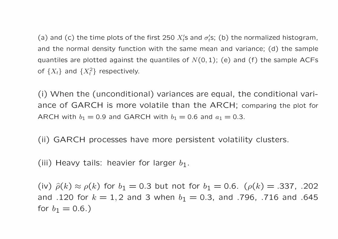
(a) and (c) the time plots of the first 250 X ′ts and σ′
ts; (b) the normalized histogram,
and the normal density function with the same mean and variance; (d) the sample
quantiles are plotted against the quantiles of N(0,1); (e) and (f) the sample ACFs
of {Xt} and {X2t } respectively.
(i) When the (unconditional) variances are equal, the conditional vari-
ance of GARCH is more volatile than the ARCH; comparing the plot for
ARCH with b1 = 0.9 and GARCH with b1 = 0.6 and a1 = 0.3.
(ii) GARCH processes have more persistent volatility clusters.
(iii) Heavy tails: heavier for larger b1.
(iv) ρ(k) ≈ ρ(k) for b1 = 0.3 but not for b1 = 0.6. (ρ(k) = .337, .202
and .120 for k = 1,2 and 3 when b1 = 0.3, and .796, .716 and .645
for b1 = 0.6.)

Bougerol and Picard (1992) proved: the GARCH(p, q) model admits
a strictly stationary solution {Xt} with EX2t = ∞ if
p∑
i=1
bi +q∑
j=1
aj = 1,
and the distribution of εt has unbounded support and has no atom at
zero.
The GARCH processes fulfilled the above equation has been unfor-
tunately called integrated GARCH(p, q) (IGARCH) processes, in anal-
ogy to integrated ARMA (ARIMA) processes (i.e. processes with unit
roots).
Note. ARIMA processes are always non-stationary while an IGARCH
process may be strictly stationary.

Estimation
Observations: X1, · · · , XT be observations for a (G)ARCH process.
Goal: to estimate the parameters in the model.
5.1 Conditional MLE.
For ARCH(p) model
Xt = σtεt, and σ2t = c0 + b1X2t−1 + · · ·+ bpX
2t−p,
if we know the pdf p(·) of εt, the (conditional) log-likelihood function
is
l({bj}, c0, σ2) =T∑
t=p+1
{log p(Xt/σt)− logσt}.
The MLEs for c0, b′js and σ2 could be obtained by maximising the
above function.

Often we use qMLE resulted from assuming εt ∼ N(0,1),
l({bj}, c0, σ2) = −1
2
T∑
t=p+1
{X2t
σ2t+ logσ2t }
Note. (i) Under some mild regularity conditions, the qMLE is con-sistent. The asymptotic normality requires more conditions such asEε4t < ∞ (which may be questionable in financial application).
(ii) For a GARCH model with
σ2t = c0 +p∑
i=1
biX2t−i +
q∑
j=1
ajσ2t−j,
it can be shown that
σ2t =c0
1− ∑qj=1 aj
+p∑
i=1
biX2t−i
+p∑
i=1
bi
∞∑
k=1
q∑
j1=1
· · ·q∑
jk=1
aj1 · · · ajkX2t−i−j1−···−jk
.

Apply truncation: define for t > p
σ2t =c0
1− ∑qj=1 aj
+p∑
i=1
biX2t−i
+p∑
i=1
bi
∞∑
k=1
q∑
j1=1
· · ·q∑
jk=1
aj1 · · · ajkX2t−i−j1−···−jk
I(t− i− j1 − · · · − jk ≥ 1).
The conditional MLE (b, a, c0) minimises
T∑
t=ν
{log σt − log f(Xt/σt)} ,
where ν > p+1.
(iii) The estimation for conditional second moments is more difficult
than that for conditional mean; the likelihood functions tend to be
rather flat (unless T is very large).

Simulation with 1000 replications for ARCH(1) with b1 = 0.9, c0 = 0.2
and εt ∼ N(0,1)
T Eb1 MSE(b1) P (b1 ≥ 1)
100 .8522 .2574 .266250 .8839 .1636 .239500 .8927 .1066 .1521000 .8980 .0814 .100
Simulation with 1000 replications for GARCH(1,1) with b1 = c0 = 0.2,
a1 = 0.7 and εt ∼ N(0,1)
T E(b1 + a1) MSE(b1 + a1) P (b1 + a1 ≥ 1)
100 .8787 .1467 .206250 .8868 .1025 .143500 .8968 .0658 .0601000 .8991 .0489 .019

(vi) To increase the fatness of tails, we may let εt have one of the
following distributions (all with tails heavier than normal):
(a) t(k): fk(x) =Γ((k+1)/2)
(πk)1/2Γ(k/2)1
(1+x2/k)(k+1)/2.
(b) Double exponential distribution:
f(x) = 2−1/2 exp{−√2|x|}.
(c) Generalized Gaussian distribution:
f(x) =k
λ21+1/kΓ(1/k)exp{−1
2|x/λ|k},
where λ = {2−2/kΓ(1/k)/Γ(3/k)}1/2.
Note. All above distributions have been normalised with variance 1.

(v) Model selection: We may use AIC or BIC to determine the orders
of model.
AIC = −2(maximised log likelihood)
+ 2(No. of estimated parameters)
BIC = −2(maximised log likelihood)
+ logT (No. of estimated parameters)
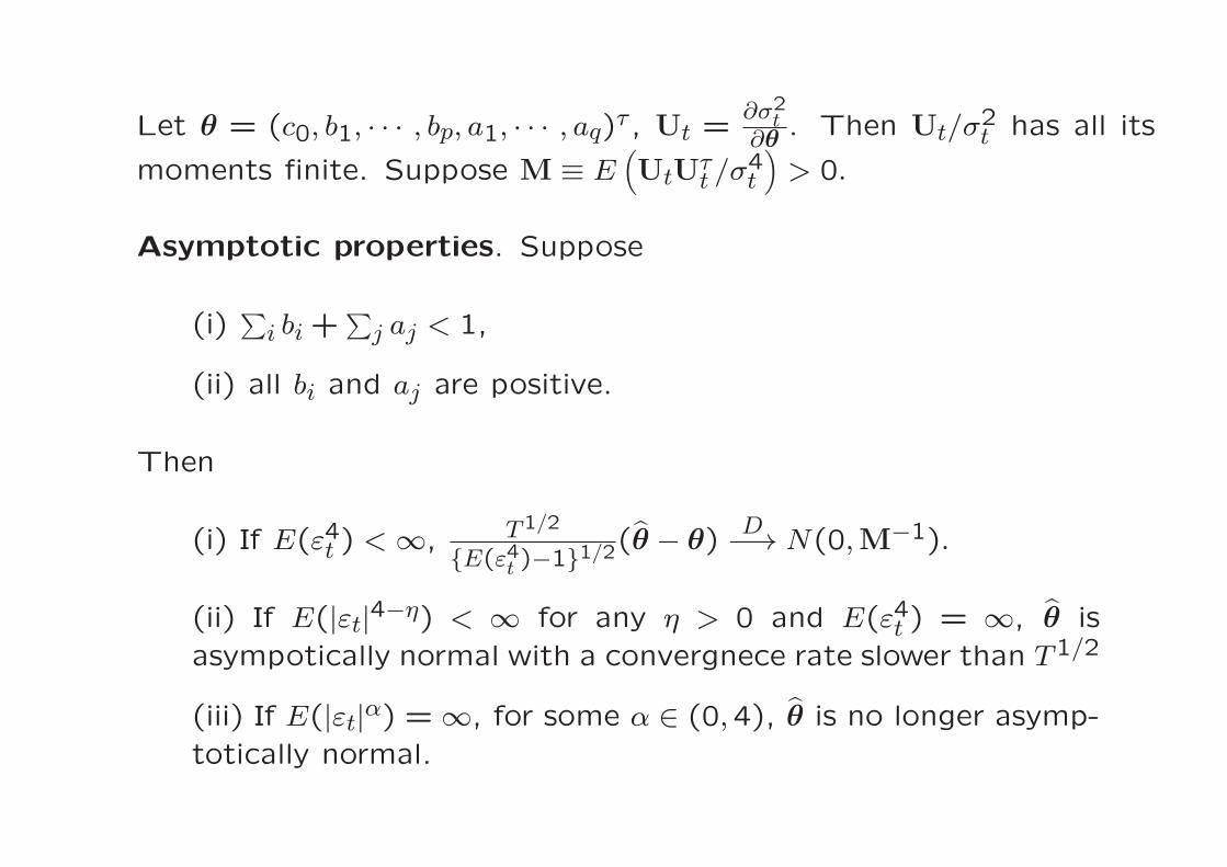
Let θ = (c0, b1, · · · , bp, a1, · · · , aq)τ , Ut =∂σ2t∂θ . Then Ut/σ
2t has all its
moments finite. Suppose M ≡ E(UtU
τt /σ
4t
)> 0.
Asymptotic properties. Suppose
(i)∑
i bi +∑
j aj < 1,
(ii) all bi and aj are positive.
Then
(i) If E(ε4t ) < ∞, T1/2
{E(ε4t )−1}1/2(θ − θ)D−→ N(0,M−1).
(ii) If E(|εt|4−η) < ∞ for any η > 0 and E(ε4t ) = ∞, θ is
asympotically normal with a convergnece rate slower than T1/2
(iii) If E(|εt|α) = ∞, for some α ∈ (0,4), θ is no longer asymp-
totically normal.

L1-estimation
Model: Xt = σtεt, εt ∼ (0,1), and
σ2t ≡ σt(θ)2 = c0 +
p∑
i=1
biX2t−i +
q∑
j=1
ajσ2t−j,
where θ = (c0, b1, · · · , bp, a1, · · · , aq)τ .
Reparametrisation: Eεt = 0, Median(ε2t ) = 1.
Note. Under the new parametrisation, c0 and bi’s differ by a common positive
constant factor while aj’s unchanged
Now
X2t /σ
2t = 1+ (ε2t − 1).
This leads to
θ1 = argminθ
T∑
t=ν+1
|X2t /σt(θ)
2 − 1|.
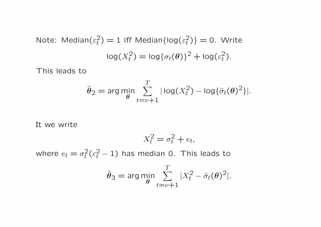
Note: Median(ε2t ) = 1 iff Median{log(ε2t )} = 0. Write
log(X2t ) = log{σt(θ)}2 + log(ε2t ).
This leads to
θ2 = argminθ
T∑
t=ν+1
| log(X2t )− log{σt(θ)2}|.
It we write
X2t = σ2t + et,
where et = σ2t (ε2t − 1) has median 0. This leads to
θ3 = argminθ
T∑
t=ν+1
|X2t − σt(θ)
2|.

Asymptotic normality. Suppose
(i)∑
i “bi”+∑
j aj < 1,
(ii) all bi and aj positive,
(iii) log ε2t has the unique median zero, and its density function
f is continuous at zero.
Then,
(i) T1/2(θ2 − θ) is asymptotically normal with mean 0
(ii) T1/2(θ1−θ) is also asymptotically normal with a non-zero
mean (i.e. bias).
(iii) The asymptotic normality for T1/2(θ3 − θ) requires more
conditions such as Eε4t < ∞.

Simulation comparison of conditional MLE and LADE
ARCH(2): σ2t = c0 + b1X2t−1 + b2X
2t−2
GARCH(1,1): σ2t = c0 + b1X2t−1 + a1σ
2t−1
with c0 = 3, b1 = 0.5 and b2 = a1 = 0.4
εt ∼ N(0,1), t3 or t4. (E|εt|d = ∞ if εt ∼ td.)
Sample size: 300 Simulation replications: 500
The average absolute error (AAE):
(|b1/c0 − b1/c0|+ |b2/c0 − b2/c0|)/2 (for ARCH(2)),
(|b1/c0 − b1/c0|+ |a1 − a1|)/2 (for GARCH(1,1)),
Estimates were obtained through exhausting search.

0.0
0.2
0.4
0.6
0.8
t(3)MLE
t(3)LADE1
t(3)LADE2
t(3)LADE3
t(4)MLE
t(4)LADE1
t(4)LADE2
t(4)LADE3
NormMLE
NormLADE1
NormLADE2
NormLADE3
(a)
0.0
0.4
0.8
1.2
t(3)MLE
t(3)LADE1
t(3)LADE2
t(3)LADE3
t(4)MLE
t(4)LADE1
t(4)LADE2
t(4)LADE3
NormMLE
NormLADE1
NormLADE2
NormLADE3
(b)

Tests for ARCH effect
Tests on GARCH models can be divided into two categories:
1. The LR tests can be constructed in the standard manner.
2. Apply the standard tests for ARMA models to the process {X2t }.

Suppose that {Xt} is a strictly stationary process defined by
Xt = σtεt, σ2t = c0 +p∑
i=1
bjX2t−i,
where c0 > 0 and aj ≥ 0.
We are interested in testing
H0 : b1 = · · · bp = 0
against
H1 : bj 6= 0 for at least one j.
Suppose the density function f(·) of εt in is known, the (conditional)
likelihood ratio test based on the test statistic
T∏
t=p+1
σt(c0, b)−1f{Xt/σt(c0, b)}
σt(c0,0)−1f{Xt/σt(c0,0)},
where (c0, b) is the (conditional) MLE for an ARCH(p) model, and c0is the constrained (conditional) MLE under H0.

Under the null hypothesis H0
2 log(ST,1)D−→ χ2
p
provided that the density function f(·) is enough smooth, and theFisher information matrix
I(c0,b) ≡(
I11(c0,b) I12(c0,b)I21(c0,b) I22(c0,b)
)= E{ℓ(Xt; c0,b)ℓ(Xt; c0,b)}τ .
exists and is positive-definite; see §4.4.4 of Serfling (1980). (Those
conditions are fulfilled for GARCH models with εt ∼ N(0,1).) In the
above expression, ℓ(Xt; c0,b) denotes the derivative of log[σ−1t f(Xt/σt)]
with respect to (c0,b).
The above asymptotic distribution under the null hypothesis is also
shared by both score test and Wald test.

The score test is also called the Lagrange multiplier test by econome-
tricians. It is based on the fact that the gradient of a log-likelihood
function should be close to 0 under a null hypothesis. More precisely,
it can be shown that under H0,
1√T − p
T∑
t=p+1
ℓ2(Xt; c0, 0)D−→ N(0, I22(c0, 0)),
where
ℓ2(Xt; c0,b) =∂
∂blog[σ−1
t f(Xt/σt)],
and I22 is defined in the above Fisher information matrix.
The score statistic is defined as
ST,2 =1
T − p{
∑
t=p+1
ℓ2(Xt; c0, 0)}τ{I22(c0, 0)}−1
×∑
t=p+1
ℓ2(Xt; c0, 0).

If εt is normal, Engle (1982) shown that the score test may be per-
formed in terms of the statistic TR2 which is asymptotically equiva-
lent to ST,2, where R2 is the multiple correlation coefficient of Xt and
(Xt−1, · · · , Xt−p), namely
R2 = Xτp+1X (X τX )−1X τ
Xp+1/(Xτp+1Xp+1),
where Xk = (X2k , X
2k+1, · · · , X2
T−p−1+k)τ , X = (1,Xp,Xp−1, · · · ,X1),
and 1 is a vector with all components 1.

§7. A case study — SP500 index
We illustrate the GARCH modeling techniques in terms of the daily
SP500 index data set in 3 January 1972 – 31 December 1999.
0 2000 4000 6000
4.5
5.0
5.5
6.0
6.5
7.0
The Standard and Poor’s 500 Index
Define the returns
Xt = 100(logYt − logYt−1), t = 1, · · · ,7075.

Graphical investigation
-20 -15 -10 -5 0 5 10
0.0
0.1
0.2
0.3
0.4
0.5
Histogram of the SP500 returns and a normal density function with the
same mean and variance.
The histogram has a long stretch on its left due to the single large
negative return — the stock market crash of October 1987. However
if we discard this single ‘outlier’, the marginal distribution seems fairly
symmetric but not normal.

Lag
AC
F
0 20 40 60 80 100
0.0
0.2
0.4
0.6
0.8
1.0
(a) ACF of returns
Lag
AC
F
0 20 40 60 80 100
0.0
0.2
0.4
0.6
0.8
1.0
(b) ACF of squared returns
The correlogram of (a) the SP500 returns, and (b) the squared returns.
There is almost no significant autocorrelation in the return series {Xt}itself, but such a autocorrelation does exist in the squared series {X2
t }.

The sample quantiles of the
SP500 returns are plotted
against, respectively, the
quantiles of N(0,1) and
t-distributions with degrees
of freedom between 7 and
3.
Both tails the empirical dis-
tribution of the returns are
heavier than those of N(0,1)
and tk for k = 6 and 7, is
considerably lighter than t3.
Therefore,
E(X6t ) = ∞, E(|Xt|3−ǫ) < ∞
for any ǫ > 0.
• •••• ••••••• •••
••••• • •• •• • ••••
•••• ••• •• • •• • •••••••• •••
• •••••
•• • •••• ••• •• •• •••• • • •• • • ••••
•• ••• • •••• •••••••• •• •• • • •••• ••••• •• • •• • •
••• •••
• • ••• •
• •• •••••••••• ••
••• •• ••• •• •• •••• ••••
•••• ••• •• ••••• ••
•••••• •••••
•••• •• •••• •
•• ••• ••
••• ••• • •• ••• ••••• •• •• •••
••• •••• •••••
•• • •••• ••
•• • •• • • •
• ••••
••
••• •
• •••
••••
••• • ••• ••
•••
• • ••
••• • • •
• •••••••••
•••
••
• •• •
••
•••••
•••• •••
••
•• •••
••
•••
•••••
•••
••
•• ••
• •••
• • •
••
•• •• •• • ••••••
•• ••••
••••
• ••• ••
••• •
• ••• ••• • • • •••
•••• •••• • •••
••••
••
••• • •
•••• •
•• • •••
•• •
• • ••
••
••
••
••
•
•••
••
•••
•••
••
•••• •
••
• •••
••••
•
••
• ••
••
••••• ••
•••
• ••••
••••
••••
••••• •
••
•• •• •••
• ••• • ••
••••
••
•• •
••• ••
••• •
•• ••
• ••
•• • •••
• ••••
•• •
••
••
•
•••
••
•••
• • ••• ••••
••
••• •
•••
•
•
••
•
••
••• • ••
••••
• • •• •
•
• •••••••
•
•••
•
•••
•
••
•
•
•••
• •
•••
•
••
••
•••• •
••
•
•
••
• •
• •
• •••
••
••
••
• ••
•
••
• •
•••
••
•• • •
••••
••
•
••
••
••••
•••••
••• •
• ••••
•
• •
••••
•••
•• •
•
• •
•
•••
•• •• •
••••
• •••
•
•• • ••••••
•••
• •
••• ••
••
••• •• ••
••
••••• •
••
••
• •••
•• ••
••• •
•••
•••••
••
•• •••
•• ••• •
••• •
• ••
• ••••• ••••
• ••
•• •••• ••••
•• •••••••
•••••
••
••
•••
•••
••
••
••••
• • • ••••
••
• ••
• ••••
••
••
••••
• • ••••• •
••
••
•••• ••• • •
••• •
•• • • ••
•••••
••
•• •• • • •••
••••••• • •
••• •••
•
••
•••
• •••
••••• • •
• •• •••••
• •••
•••
• • •••
•••• •
•••
•• •••
• ••••
• ••
•• •• •
••
• • •••• •• •••••
•• • •
•••• • •••
••
•• • •• ••
• • •• • •••
••
• •• • ••• •••
•• •• ••
• •• ••• ••••• • • ••
••• •••
• •• • •••• ••
•• • • • •
• • ••• •• • ••••
•• • •• • ••
•• • ••••
•
•• •• •
••• •••
••
••
• •••
••
•• • •• •
•• •
• • ••••• •••• ••••••••
•••
•••• •
•• •• •
••••
••
•••• • •• ••• ••••••
•• ••• ••• • • •
• ••••••• •••••• •• •• • •
••
•• •• •• •
• •••• •••
••• ••••• • •
• • ••• •••
• •••
• ••
••
•••• •• •
• •• ••• • ••• • •• •• ••• • • • •••• •• •
••• •
• • ••• • •• • •• ••• ••••
••
••• •••
•• • • •••• •• •• •• • •••• • ••••• • •••
•••••
••••• • • ••• •
•••
•• • ••
•••••
•••••
• • ••• •• •• • • •••• ••
••••• •• ••• • •
• •• • ••
• •• ••• •
••• •• •• •• ••
•••
••••••
•• •• • ••
• • •••••••
• •• •••••
••
•• •
••••
•••
•• ••
•• ••••••
• ••
•• •• ••• ••
•• ••• ••• •
•• • ••
•••••••
• •• ••••
••
••• • ••• ••
•••• ••
•••• ••••• •••• • •• • •••
••••• •• ••••• •
•• ••• ••• •
••
• •• • •••
•• •
•••
•
•
••
•••• •
••
• •••• •••
••
• ••
••••
••• ••
•
•••••
• • • • •••• •
•• ••
•• ••• •
•••
•••••
••
•••• ••••
••• • •
•• ••
•• • •• ••• • ••
•••••
•• •••
•• ••• •
• ••• •
• • • ••• • ••••••
• ••
•• • ••
• • •• • •••
••••••• • •
• ••• •• ••••
••••
• • ••••• • •
• •• •• • •••• •••• •
•••
••• •• • ••• • ••• •• •
• •••
•• ••••
••• • ••
•••
• • •
••
••••• ••
•• • ••
•••
••••••
• • •
•• •
• •• • •
•
• ••• ••• •
• •• ••••
• • •• •••• ••
••
••
• •• • ••• • ••
•••
••
••
••
• •••
•••
• • •
•
• ••
••
••
••
•• ••
•••
•
•
••
• •
•
•••
••
• ••
•
••
••• •• •••
•
• •••• ••
• ••
•••
••
•• ••• •• •••
•
•• •
•• •• • •
• ••• •• •
• • •• •
•••
••• •
••
•
••
•••••••• •
••• •• • •• •
• ••
•
••
• ••
• •••• • •
••••••• • • •
•• •
••
•••
••• • •
••
•••
••
• ••
• ••
••
•••
• • •
•••
••
•••
••
•• •
•••
•
•••••
••
••
• • •• •
•• ••
••••
••
• •••• • •••
••• ••
•• ••
•
•• ••
••• • •
•••
• •• • ••••
•• •
•••
•
••
• ••• •
•
•
•••
•••••• •••
• ••• •
• ••••
•• •••
• • •••
•• •••• •••
•••• •
••• ••• • •
• ••
••
•••
• ••••• •••• •• •• •• •
•••
• • •• • ••
• • •••
• •• ••••
•••
•
• ••
••
• •• ••
•••
•••• ••
•• ••
••• •
•••
••• ••
•
•• •
•••• •
•••
••••
• ••
• ••••
••
• ••
•• ••
••
• •• • •••
•••
••• •• •••
•••
•• • •
•••
•••• •
•• •• •
••
•
••
• •
••
•• ••• ••
••
•• • ••
• • ••
•••••
••••
••
• ••
•••••
• •• •• •• ••••
••••
• •••• •• ••
••
•• •• •• • •••• •• • ••
••••
••
•••• • •
• •••
••••• • • •
••••
• •••• •••••
••
•
•• •• • •••
•
•
••
••
•
••
••
•
•
• •
••
•••• •
•••
•
• •• ••• •
•• •
••• •
••
• •
•
••
••
•
•••
•••
•
••
•
•
••
•• •
••
••
•••
•
•
•••
••
••• •
• ••
•
•
•• •
•
••
••
•
••
•
••
••
••••••
••
••
•• •
•• • ••
• ••
• ••• • •
•
••
••
•••••
•
•• •• •
•• • •
••
••• ••
• •••• • •• • •• •
••
• ••
••
••
•• •• •
• •• • ••
••• • • •••••• •••
• •• • •• • •
••••• •
••
••••
•• •
••
• •• • •
•
•• • •
• ••• •
••
••
• •• • ••
••
•••• •
•• ••
• ••
•••• • ••
••••
•• •
• ••• • • • •• •
•• •• •
•• •• • •• ••
•• •• • • •
••
••
•••••••••
••
•• •• •• • •••••••
•••
••• ••••
••• ••• • ••••••
• • •••• •
•••
•• •
••
• ••• • ••
•
•• ••
••••
••
•• • ••
•••
•• ••
••• • ••
•• ••
••
••• ••
•• •• •
•••
•• •
• •• •••
• ••••••
•••
••
••
• •• • •• •
•• •
• ••••••• •
• ••
••
••••
••••••••
••
•••
•••
•
•••••• •
•• • •
•••• •
• ••
• • •••
••• • •• • • ••
•• •••••• •• ••
• •
•
•• • ••• ••
••
• • •• •• •• ••
• •••
•
••
•• •• ••
•• ••••••
•
••••
•• • •• ••
•• ••
••
••• ••
••
• ••••••••• ••
••
••• •••• •
•• •
•• •
• • •• •• ••
••
• ••• • •• •••• •• • ••••••• •• •• ••• ••
• •• •• • ••• • • • •
•••••• •
•• •• •
• •••••
• •• ••
• •• ••••••
••••••
•••
••• • •••
• •••••
• ••• • ••• • ••
• • • •••••• • •••• • • ••• •
••
••••
•• ••• • •• • •
••
•• • •••• • •••
•• ••• •
••
••
• •• ••
•• • •••
••
•••• ••
••• • • •
• •• •••
•••
•
•• • •• ••••••
• •• •••
••• • • • •
• • • ••
•
•••• •
••• • • •• •
•••
•
••• •
•
••
••••
•••
••
••
• •••
•••
• • • ••
••
•••
•••••
• ••
••
•• •••••
••••
•• ••
••
•••
•
•••• • ••••
••
•••••
•••• ••••
••
•••
••• •••••••••
•• •
•
••• •
•
• •
• • ••
•
•
••• •••••
••
•• ••• ••
•• • ••
•••
•• •
•• •• • •
• •••• • • •••
••
•
•••
••••••
••• •••
• • • •• •
•••
••• ••
• •• •••••
••• •••
•
••
••
• ••
•••
••••
•• •
••••
• •• •• ••
••••
• ••••
• ••••• •
••
•• ••
•
••
••
••
••
•
•
••
•• • • •
• ••
•••••••
••
••
••
• •• ••
••
••
•• • •••• •• •••
•• •
••
••
••• •••
• ••••
•• ••• •••••• ••
•••
•• •
••
••
••
••••
•••••
•• •
•• •
•••
•
•• • •• •
•••
•
•• • •
•
• •
•
•
•
•
•
•
•
•
••
•
••
•
••
•
••
••
•
•
•
•••
••
•
••
•
•
• ••
•
••
••
•
•
•••
••
••
•
•
•• •
•
•
•••
•
••
•
••
•
••
••
••
••••
••
•• •
••••
••••
•
• ••• • ••
•
•••••
••••
•••
••
••
••
••
• ••
•
•••• ••••••• • •
• ••••
••
••••
•••
•• ••
••
•••
•
•
•••
••
••
•• •
•••
••
••
•
••• •
••• •
•••
••••
•
••
•• ••••••••
•••••
••
•
•• •
•••
•••• •• • •
••
•••• ••• •
•••• ••
•••
••• • •
•
••• ••
••••••
•••
• •
•• •
•• •• • •
•• • •
• ••••• •••••
• •• •• •• • •••
••••• •••••
••••
•• ••• •
•• •••
•••••
•• ••
••
••••
•• •• •••
•• • •
••
••••••• ••
• •••• ••
•
••
•••
••• • •••• •••• • • •
••
•••
•••
•• ••
•• ••
•••••• ••
•••• ••
••
••
•••• ••••• •••
••
•• •
•••
•• •••
•••
•• •
••• ••
••
•• •
••• •
•• • •• •• •
••••• •• • • •
• • ••• •••••
•
•
• ••
•• ••• •
••
•• •
•• •
•••••• •
• • •••••• •
•• •• ••••• •
•• • • •
• •• ••
••••
• ••
••
••
••
•
••••••
•• ••
••
• ••
•• •••
••••
•• ••
••
••
••
••••
•••••
•••••
•• •• ••• •••
• •••• ••
••• •• •••••
••
•• •••••••
••• • •
••••• •
•• ••
•• •• • •
••• •••
•••
•••••••
••• •••
•••••
•
•••
•
•••
••
•
• ••
••
••
•
•• •
••
• • •• •
•••
••
•
•
••
••
••
•••
•••
••
••
•••
• ••• •
••• ••
••
•••
••
•• •
••• ••••
••• •
•• ••
••• •
••• •
• ••
• •••
••
••
•••
• •
•
•••
• ••••
•••
•••
••
•
••
•
••
•• • •
•
••
••
••••••
•• ••
••• • •
•• •
•
•
• ••
••
••••
••
•• •••
••
•• •
•••••
•
•
•• •
••• •••
• •• ••
• •• ••• •
••
•• ••
• •
•• • •
•
••
•• •
• • • •••••
••• • •• • ••• •••
••• • •••••
••
• ••••
••• • • •••
• ••
•• •••••••• ••••• • •
•••
•••• ••• •• •••••••• • •
• • •••
•
••
• •• •
•••
••••
•••••••• •••
•• •
••
•• •• • ••• ••
•• ••••
••••
••
•• •
••••• •
• ••
••
• •••
•• • ••• • • •• • •• •
• • •••• ••
• •••
• •
••
•••••
••
•• •• • • ••
••• • •
• •••• •
•••
• ••
• ••
•• ••••••••
••
•• ••• ••
••
• ••
• ••• •• ••• ••
••••••• ••••• ••• • •••
• •••• •• •• •••••
• ••
•
••• •
••
• ••
•• ••• • ••
••
•••• • ••••••
• ••••
••• •• •••••
•• ••
•••••• • • ••••• ••• •
••• ••• •• •• •
• • •• • ••••••• •
•• •• ••••••• ••
••
•• ••••
••••
•• ••
• •••
••••
•• •• ••
•••••
•• •••
••• ••• •• •••
• •• ••••• • •••
••••
••
•• •••
•••••••• ••• ••
••••
•• •• ••••
••
• •• ••• • ••••••••
••••• • •• •• • •• ••••
•••• •••• •• • • ••• •• •• •
••••
••• ••••• •••••••• ••• ••• •• ••
••••• •
• ••
•• •••
•••• •• •••••• • •• • • •• •• ••••• • ••• • •
• •••• ••••• • • •• •
•••
•
•• ••
•• •••••
••
••• •• ••• ••
••• •••• •••• •••
••
•• •
••
• • ••• •••
••
•••••• •••
••
••••••
•• ••••• •• •• •• •• •• •
••••
••
•• •
•••• ••• • • ••••• •• ••• • ••• •• • •• ••
••••• •• • •
••
• •••• •• •• • •
•• •
•• •• •• •
• •••
•• • • •• •••• •
• •••• •
••• • •
•• ••••
•• ••••
•• •••••
•••••
• •••
• ••• ••• •
• •• • •• •• ••••••••• •• •• •• •• • ••• •• •• • ••• • •••
••
• • •••••
•• ••
•••• •••••••• • •••••• ••
• •• • • •• •••• •
••• •• •• • •••
••
•••••
••
•• ••• ••• •
•• • •••
••• • •• • ••
•••••
•• •••
•• • •• •• •• • •• •••••
•• •• •• •• • •• •• • ••• •• •• ••• • •
• • ••••
•• •• ••• • • ••••• •
•• •••
••• • ••••••••
••••
•• •• ••• • •••
• ••• •• •
•
••
•• ••• • ••• • •••
••••
• • ••••
••• ••••••• •
• ••••••
• ••
• •••• ••
• •
•
•• •••
••• • •• •
• •••
••••
••
••••
• •• ••• ••••••
• •••
•• •••• •••
•• •
• ••
• •••
• •••••• •• •• •••••• •
• ••
•••
••
•
•• •
•••• ••
••• • •
• ••• • ••
•• •••••
••••• •••
•• •
• •• •••• • ••• ••••• ••
•••• •
••• •• ••• •• •••• •• • • •
•••• • ••• •••• •
•• ••• • ••
••••
••
•••
•• •••••
••
• ••
••••
• • •• ••• • • •
• ••• •
••
••
•••
••
•••
•••• •
••
••
• •••
•
••• •• • •
• •
••
••
••••
• •
•
• ••• •
•
••••
••
••
• •
••
•••
•• •
•• •
•••
••• •••••
••• •
•••••
••
•
•
• •••
• •••
••
••• • ••
••
•••••
• •••
•• ••
•
•• • •
•
•••
•••• •
• •
•
• •• ••• •
••
•
• •• ••••
•••
••• • •• •• •••••
• ••
••
•
•
••
••
•••• ••
•
•• •
•• •
••
•• ••
• ••
••••
••
••••••
• ••
••• ••
• •••
••••
• •
•• • ••••
•
••••
••
•• •• • ••
•••
•••• •••
•
•••••
•• •• ••
•• •• •
•• •••• •
•• ••
•
•• ••
•••
•• ••••••
••
•••• • • •••
•• •
• • ••
• ••••
••
•
• ••• •
••• •••
••
••
••
•••
••••
••
•• •
••
•
••
•
•••••
•
••
•••••
•••
•
•
•
•
•••
•
••
••••
•
• • •
•
•
• ••
••
•
••
• •
••
••
•
••• • •• ••
•••
• • ••• •• •
• •• • • ••
• ••
•
••
•
••
• ••
•
•
••
•• ••
•
•••
• ••• •
• ••
••
•
•••
••
• ••
••••
•
••
•
•
••
•
•
•
••
•
•• •• ••
•• •
•• • ••
•••
•
••
•
••
•
•
•••
•
•• •
• ••
•••
•
•••
• ••• ••
•
•
•
••
••••
•
•••
••••
•
•
•• • •
••
••
• • • ••
•• •• •
••
• ••••• •• •
•• • •••
•
••
•••
•• •
••••
• ••
••
•• •
••• •
••
• •••
••
•
•• •• •••••
••
•
•
•• ••
•
••
••
•
••
•••
•
•
•••
••
•••
••
• •••••
••• •
••
••
• ••
••••
• ••
•• • • •••••••
••
••• •• •
(a) Returns vs Normal
normal quantile
quan
tile
of r
etur
ns
-4 -2 0 2 4
-15
-10
-50
510
•••••
•••••••••••
••••••••••••••••••••••••••••••••••••••••••••••••••••••••••••••••••••••••••••••••••••••••••••••••
••••••••••••••••••••••••••••••••••••••••••••••••••••••••••••••••••••••••••••••••••••••••••••••••••••••••••••••••••
•••••••••••••••••••••••••••••••••••••••••••••••••••••••••••••••••••••••••••••••••••••••••••••••••••••••••••
••••••••••••••••••••••••••••••••••••••••••••••••••••••••
••••••• •
•
(b) Returns vs t(7)
quantile of t(7)
quan
tile
of r
etur
ns
-5 0 5
-15
-10
-50
510
•••••
•••••••••••
•••••••••••••••••••••••••••••••••••••••••••••••••••••••••••••••••••••••••••••••••••••••••••••
•••••••••••••••••••••••••••••••••••••••••••••••••••••••••••••••••••••••••••••••••••••••••••••••••••••••••
•••••••••••••••••••••••••••••••••••••••••••••••••••••••••••••••••••••••••••••••••••••••••••••••••••••••
•••••••••••••••••••••••••••••••••••••••••••••••••••••••••
••••••• •
•
(c) Returns vs t(6)
quantile of t(6)
quan
tile
of r
etur
ns
-5 0 5
-15
-10
-50
510
•• •••
•••••••••••
•••••••••••••••••••••••••••••••••••••••••••••••••••••••••••••••••••••••••••••••••••••••
•••••••••••••••••••••••••••••••••••••••••••••••••••••••••••••••••••••••••••••••••••••••••••••••
•••••••••••••••••••••••••••••••••••••••••••••••••••••••••••••••••••••••••••••••••••••••••••••••
••••••••••••••••••••••••••••••••••••••••••••••••••••••••
•••••• • •
•
(d) Returns vs t(5)
quantile of t(5)
quan
tile
of r
etur
ns
-10 -5 0 5 10
-15
-10
-50
510
•• •••
•••••••••••
•••••••••••••••••••••••••••••••••••••••••••••••••••••••••••••••••••••••••••••••••••
••••••••••••••••••••••••••••••••••••••••••••••••••••••••••••••••••••••••••••••••
•••••••••••••••••••••••••••••••••••••••••••••••••••••••••••••••••••••••••••••••••••
••••••••••••••••••••••••••••••••••••••••••••••••••••
•••••• • •
•
(e) Returns vs t(4)
quantile of t(4)
quan
tile
of r
etur
ns
-15 -10 -5 0 5 10 15
-15
-10
-50
510
•• •••
•••••••••••
••••••••••••••••••••••••••••••••••••••••••••••••••••••••••••••••••••••••••
••••••••••••••••••••••••••••••••••••••••••••••••••••••••••••••••••••••••••••••••••••••••••••••••••••••••••••••••••••••••••••••••••
•••••••••••••••••••••••••••••••••••••••••••••••••
•••••• • •
•
(f) Returns vs t(3)
quantile of t(3)
quan
tile
of r
etur
ns
-20 -10 0 10 20
-15
-10
-50
510
Testing for conditional heteroscedasticity
Fix the conditional mean for the daily returns at 0, see J.P. Morgan’s
RiskMetrics (Morgan, 1996, p.92). Fitting a GARCH model to the
return data.
The likelihood ratio test for ARCH effect rejects the null hypothesis
(of homoscedasticity) with p-value virtually 0 for
• εt ∼ N(0,1), or tk for k = 3, · · · ,8, and
• p = 1, · · · ,4.

Fitting a GARCH model with Gaussian innovation
Suppose εt ∼ N(0,1), both AIC and BIC selected the GARCH(1,3)model with
σ2t = 0.015+ 0.112X2
t−1 +0.492σ2t−1 − 0.034σ2
t−2 +0.420σ2t−3,
with AIC= 17792.2 and BIC= 17826.5. The standard errors of the
five estimated coefficients on the RHS of the above equations are
0.002, 0.004, 0.070, 0.083 and 0.055 respectively. The coefficient
-0.034 in the above model is not significant since the corresponding
p-value of the t-test is 0.341. Therefore the term containing σ2t−2
may be removed from the model.

The time plots of (a) the
SP500 returns {Xt}, (b)
the estimated conditional
standard deviations {σt}, and
(c) the residual {εt = Xt/σt}.The estimates were derived
based on a GARCH(1,3)
model with εt ∼ N(0,1).
The residuals are less
volatile.
(a) Returns of the S&P 500 Index
t0 2000 4000 6000
-20
-10
05
(b) Estimated conditional STD
t0 2000 4000 6000
24
68
(c) Residuals
t0 2000 4000 6000
-20
-10
05

0 20 40 60 80 100
0.0
0.2
0.4
0.6
0.8
1.0
(a) Residuals
0 20 40 60 80 100
0.0
0.2
0.4
0.6
0.8
1.0
(b) Sq-residuals
••
••••••••••••••••••••••••••••••••••••••••••••••••••••••••••••••••••••••••••••••••••••••
••••••••••••••••••••••••••••••••••••••••••••••••••••••••••••
••••••••••••••••••••••••••••••••••••••••••••••••••••••••••••••••••••••
•••••••••••••••••••••••••••••••••••••••••••••••••••••••••••••••••••••••••
•••••••••••••••••••••••••••••••••••••••••••••••••••••••••••••••••
•••••••••••••••••••••••••••••••••••••••••••••••••••••••••••
••••••••••••••••••••••••••••
•••
•
(c) QQ-plot
Normal quantile
Qua
ntile
of r
esid
ual
-4 -2 0 2 4
-10
-50
5
The correlogram of (a) residuals from the fitted model, and (b) the squared
residuals. (c) The QQ-plot of the residuals verses a normal distribution.
No significant autocorrelation in both the residual sequence and its
squared sequence. In fact the residuals pass the likelihood ratio test
with normal conditional density.
However the fitting is not adequate; both tails of the empirical distri-
bution of the residuals are heavier than those of a normal distribution.

Fitting a GARCH model with εt ∼ td
Fitting a GARCH model with εt ∼ td, d is estimated by the MLE. Both
AIC and BIC selected a GARCH(1,1) model with
σ2t = 0.007+ 0.047X2t−1 +0.945σ2t−1,
and d = 7.41 with standard error 0.487. The standard errors for
the above model are 0.001, 0.005 and 0.005. AIC= 17411.7 and
BIC= 17439.2.

The time plots of (a) the
SP500 returns {Xt}, (b) the
estimated conditional stan-
dard deviations {σt}, and (c)
the residual {εt = Xt/σt}. The
estimates were derived based
on a GARCH(1,1) model with
t-distributed εt with the esti-
mated degree freedom 7.41.
(a) Returns of the S&P 500 Index
t0 2000 4000 6000
-20
-10
05
(b) Estimated conditional STD
t0 2000 4000 6000
12
34
5
(c) Residuals
t0 2000 4000 6000
-20
-10
05

0 20 40 60 80 100
0.0
0.2
0.4
0.6
0.8
1.0
(a) Residuals
0 20 40 60 80 100
0.0
0.2
0.4
0.6
0.8
1.0
(b) Sq-residuals
•
•
•
•••••••••••
•••••••••••••••••••••••••••••••••••••••••••••••••••••
••••••••••••••••••••••••••••••••••••••••••••••••••••••••••
•••••••••••••••••••••••••••••••••••••••••••••••••••••••••••
•••••••••••••••••••••••••••••••••••••••••••••••••••••••••••
••••••••••••••••••••••••••••••••••••••••••••••••••••••••
•••••••••••••••••••••••••••••••••••••••••••••••••••••
••••••••••••••
•
(c) QQ-plot
Quantile of t(7.41)
Qua
ntile
of r
esid
ual
-6 -2 0 2 4 6
-10
-50
5
The correlogram of (a) residuals from the fitted model, and (b) the squared
residuals. (c) The QQ-plot of the residuals verses t-distribution with d.f.
7.41.
No significant autocorrelation in both the residual sequence and its
squared sequence.
The fitting appears adequate.

Estimation of VaR – extremal quantiles
Why important to have a good fitting at the tails? — Estimation of
VaR
For α ∈ (0,1), the 100α%-th (conditional) quantile is defined as
xα = inf{x : P (Xt ≤ x|Xt−k, k ≥ 1) ≥ α}.
An extremal high quantile xα with α very close to 1 (or an extremal
low quantile xα with α very close to 0) represents the potential ‘loss’
at the probability α (or 1− α).
For a GARCH process, xα = σt xα,0, where∫∞xα,0
f(x)dx = α, and f(·)is the pdf of εt.

For the SP500 returns, the fitted GARCH(1,3) with Gaussian innova-
tion is inappropriate for a VaR estimation. The GARCH(1,1) model
t-distributed innovation would be better.
With εt ∼ t7.41, xα,0 = 2.952,3.434 and 4.656 for α = 0.99,0.995 and
0.999 respectively.
However it may still underestimate the low quantiles of the returns as
the left tail of the innovation distribution may be heavier than that
of the t7.41.

Other volatility models
ARCH and GARCH models may catch three stylized features: heavy-
tails, volatility clusters, and aggregational Gaussianity — due to CLT
for martingale difference.
However, GARCH models, in their classic form, fail to catch the styl-
ized features asymmetry and long-range dependence.

EGARCH
Exponential GARCH model that specifies the model
Xt = εt exp(ht/2), ht = γ0 + γ1ht−1 + g(εt−1),
where
g(x) = ωx+ λ(|x| − E|x|). (1)
In contrast to the form of σt in the GARCH model, the value of the
function g(·) depends on both the size and the sign of its argument.
As a result, EGARCH responds nonsymmetrically to random shocks
εt.
It is rather straightforward to identify the properties of the process
{ht} and therefore also those of {Xt}. Note that {g(εt)} is i.i.d. pro-
vided {εt} is i.i.d. Therefore {ht} is a causal linear AR(1) process if
|γ1| < 1.
For further discussion on EGARCH models, see Bollerslev, Engle and
Nelson (1994).

FIARCH
In order to model the persistent correlations in squared returns, at-
tempts have been made to construct long-memory ARCH type mod-
els. Similar to FARIMA models, we define a fractionally integrated
ARCH (FIARCH) model as
Xt = σtεt, σ2t = c0 + {1− (1−B)d}X2
t−1 = c0 + b(B)X2t−1,
where d ∈ (−0.5,0.5), and b(·) is a polynomial with hyperbolically
(rather than exponentially) decaying coefficients. Although a FIARCH
model is in the form of ARCH(∞), the slow-decaying coefficients
cause the long-term autocorrelation in the series {X2t }.
For further discussion on FIARCH processes, see Baillie, Bollerslev
and Mikkelsen (1996), Ding and Granger (1996), and Mikosch and
Starica (1999).

ARCH-M
In finance theory, the relationship between risk and return plays a
predominant role. If we take conditional deviation as a measure for
risk, it is possible to use risk as a regressor in modeling returns. Engle,
Lilien, and Robins (1987) proposed the ARCH in mean (ARCH-M)
model
Xt = g(σ2t , θ) + εtσt,
σ2t = c0 + b{Xt−1 − g(σ2t−1, θ)}2.
A commonly used parameterization is the linear one: g(y, θ) = θ0+θ1y.
See Hong (1991) for its statistical properties.

Stochastic Volatility Models
An alternative for modeling conditional heteroscedasticity of financial
returns.
A survey: Shephard (1996)
Basic idea: introduce a latent process to represent the random and
uneven flow of new information that is too complex to be modeled
as a function of the lagged values Xt−1, Xt−2, · · · only.
A general form of model:
Xt = εtg(ht) and ht = a0 + a1ht−1 + et,
where {εt} ∼ IID(0,1), {et} ∼ IID(0, σ2e ), {εt} and {et} are independent,
and g(·) > 0 is a known function.

When |a1| < 1, {ht} is strictly stationary with
µh ≡ E(ht) =a0
1− a1and γh(k) ≡ Cov(ht, ht−k) =
σ2e1− a21
a|k|1 .
This, in turn, also ensures that {Xt} is a strict stationarity process.
The most popular form (Taylor 1986);
Xt = εt exp(ht/2), ht = a0 + a1ht−1 + et,
where both {εt} and {et} are Gaussian white noise. Now {ht} is a
Gaussian AR(1) process. Therefore, we may derive that, for all k ≥ 1,
E(X2kt ) = E(ε2kt )E{exp(kht)} =
(2k)! exp{kµh + k2σ2h/2}2kk!
,
Consequently, the kurtosis of Xt fulfills the inequality
κx = E(X4t )/{E(X2
t )}2 = 3exp{σ2h} > κε = 3.
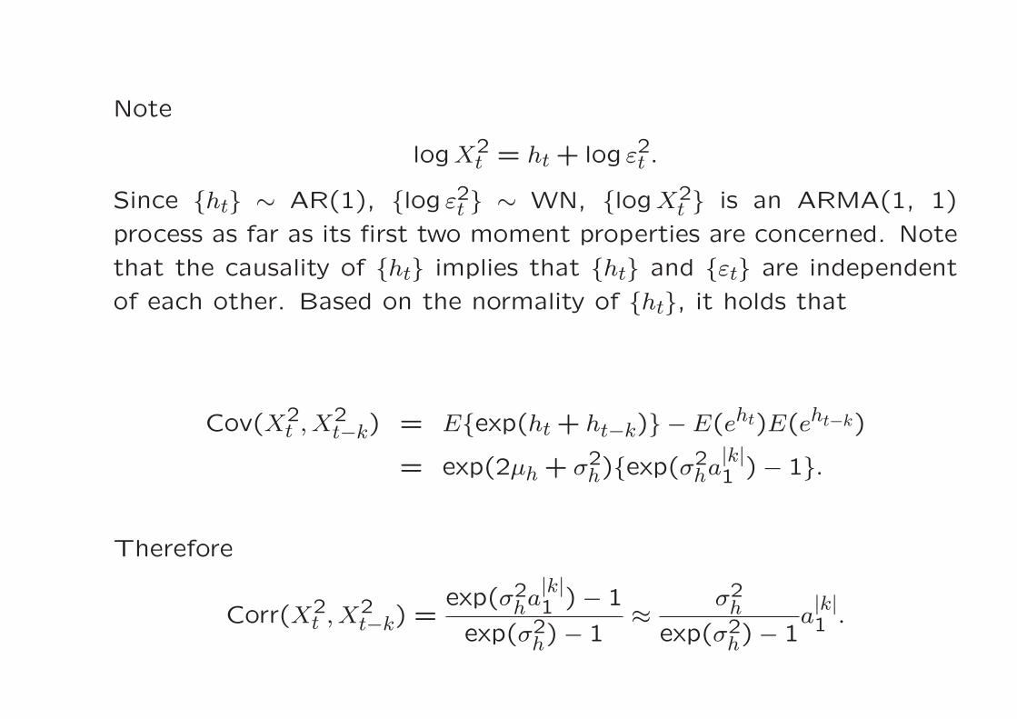
Note
logX2t = ht + log ε2t .
Since {ht} ∼ AR(1), {log ε2t } ∼ WN, {logX2t } is an ARMA(1, 1)
process as far as its first two moment properties are concerned. Note
that the causality of {ht} implies that {ht} and {εt} are independent
of each other. Based on the normality of {ht}, it holds that
Cov(X2t , X
2t−k) = E{exp(ht + ht−k)} − E(eht)E(eht−k)
= exp(2µh + σ2h){exp(σ2ha|k|1 )− 1}.
Therefore
Corr(X2t , X
2t−k) =
exp(σ2ha|k|1 )− 1
exp(σ2h)− 1≈ σ2h
exp(σ2h)− 1a|k|1 .
The approximation holds for large |k|, which may be justified by a
Taylor expansion. Note that the term on the RHS of the expression
above is an ACF for an ARMA(1, 1) process. In this sense a stochas-
tic volatility process behaves in a manner similar to a GARCH(1, 1)
process.
Statistical Inference: difficult due to the lack explicit likelihood func-
tions
Generalized method-of-moments estimates for parameters: Hamil-
ton (1989)
Kalman filter based on estimation for {ht}: Melino and Turnbull (1990),
Harvey, Ruiz and Shephard (1994)
MCMC approximate likelihood methods: see references in Shephard (1996)