modsim

7/14/2019 modsim

http://slidepdf.com/reader/full/modsim 1/94

1

Mineral Technologies International, Inc.

Modeling and Simulation of Mineral

Processing Systems

An online tutorial for learning Modsim

Course software

You should be a licensed Modsim user or have the student version of Modsim thatis distributed with the book Modeling and Simulation of Mineral ProcessingSystems, by R.P. King.

We will be using the virtual laboratory later in the course. You will need to installthis on your machine and you can download it from here.

Virtual laboratory

Here are a couple of useful utilities for you to download from this part of the coursesite. These are listed below and feel free to help yourself.

1 SI unit converter

A conversion routine to convert from obsolete units into the SI system. You can

use it also to convert back from SI to whatever system you like to use or see. Thiswill help when you want to check the values that MODSIM displays on its datainput forms. Remember that MODSIM always displays in SI units except on finaloutput where you can choose your units in the output format. When you install thisutility, I recommend that you add it to the Accessories group in your Programsfolders list in Windows (that is the group where you usually find Notepad, Paintetc). You do this during the installation. Double click on Accessories in the lower frame when you are asked to select the Program Folder. This makes the utility veryeasy to find even if you are running another job like MODSIM. The file that youdownload is a self installing executable so just download it to a convenient folder on your hard drive and then run it to do the installation.. Remember, as always, to

close down all applications before you do an install.

2 Graphics for Mineral Processors.

This utility allows you to plot graphs in any of six standard coordinate systems -arithmetic, linear-log, log-log, Rosin-Rammler, log-normal and logistic. Thesecoordinate systems are described in Technical Notes 2 where you can see someexamples. You can also plot truncated distributions if you know the truncation size.

http://www.mineraltech.com/MODSIM/ModsimTraining/Software/SETUPVLab.EXE


http://www.mineraltech.com/MODSIM/ModsimTraining/Software/SETUPSIUnitConverter.EXE



http://www.mineraltech.com/MODSIM/ModsimTraining/Software/SetupPSD.exe






7/14/2019 modsim


2

Module 1

If you have arrived here on your first visit, and you are not familiar with a WebCTcourse site, you should read at least some of the information in the courseinstructions.

This module is designed to introduce you to the graphics editor in MODSIM. Theeditor is used to draw and edit flowsheets and it is necessary to become fluent withthe editor in order to use MODSIM effectively.

If you have never used MODSIM before you should look at the first few viewlets inthe MODSIM TRAINER

The exercises are grouped into sections for easy reference.

Drawing operations.

Editing operations.

You can read a short description of simulation in Technical Note 1.

You can now complete assignment 1-1 which can be found in the drop box.

Drawing operations

These exercises will give you some practice with the drawing operations that are used in thegraphics editor.

Exercise 1-1 Drawing the unit icons.

Exercise 1-2 Changing icon size.

Exercise 1-1

Open a new job in MODSIM and draw one copy of each of the unit icons. You willnot be able to fit them all on to a single sheet. When you have filled a sheet, closethe job without saving it and start a new job. Before closing the flowsheet, add anannotation to each icon and finally use Move on the Edit menu to rearrange iconsand annotations to make a neat drawing like those shown below.

http://www.mineraltech.com/MODSIM/ModsimTraining/Module1/FrmDrawingOperations.html


http://www.mineraltech.com/MODSIM/ModsimTraining/Module1/FrmEditingOps.html


http://www.mineraltech.com/MODSIM/ModsimTraining/Module1/Simulation.PDF



http://www.mineraltech.com/MODSIM/ModsimTraining/Module1/FrmExercise1-1.html









7/14/2019 modsim


3

7/14/2019 modsim


4

Exercise1-2

Start a new flowsheet and draw three stockpiles of different size.

7/14/2019 modsim


5

Exercise 1-3

Draw two vibrating screens on a new flowsheet with one in the reflectedorientation.

Exercise 1-4

Draw several conveyor belts of different lengths and in different orientations.

Editing operations

Here is a simple exercise to practise editing functions in the graphics editor.

Exercise 1-5 Re-arrange a flowsheet.

Exercise 1-5

Start MODSIM and retrieve the Exercise 1-5 job from the Internet.

Edit the flowsheet and transform it as shown below.




7/14/2019 modsim


6

Figure 1 An untidy flowsheet.

7/14/2019 modsim


7

Figure 2 This one is much neater. Note that the feed stream was not deleted. Thisis good practice because deleting the feed stream will delete its associated data aswell. That will mean specifying the data again.

Module 2

Data specification.

Before the operation of a plant can be simulated it is necessary to specify preciselythe characteristics of the material that is to be processed and the parameters thatdefine the behavior of the individual unit operations in the flowsheet.

MODSIM uses the population balance method to model the operation of the units.This method requires the particulate nature of the solids to be specified usingdistribution functions. The particle size distribution is familiar and this is the basicdistribution function that is used. However it is usually necessary to describe other

properties of the particles as well as the size and provision is made for this as well.The basic principles of distribution functions and population balance methods aredescribed in Chapter2 of the textbook or in Technical Notes 2

MODSIM makes a clear distinction between data that is needed to describe the oreand the data that is necessary to define the behavior of the unit models.

The objectives of this module are

1. Learn to specify the properties of the ore - the system data.

2. Learn to specify parameters for the unit models.

3. Learn to find and analyze the data produced by the simulator.

System data

The system data includes any information that applies to the flowsheet as a whole.This includes information that MODSIM needs to set up its calculation algorithmssuch as for example the number of size classes that it must use for all calculations,the number of minerals that it must keep track of and the liberation characteristicsof the minerals in the ore. In some cases additional physical properties must bespecified as well. The following exercises will illustrate the procedures for specifying these data.

Exercise 2-1: Basic system data and the particle size distribution of the feed.

Exercise 2-3: Data for multi-component ore

http://www.mineraltech.com/MODSIM/ModsimTraining/Module2/TechnicalNotes2.pdf



http://www.mineraltech.com/MODSIM/ModsimTraining/Module2/FrmSystemData.html



http://www.mineraltech.com/MODSIM/ModsimTraining/Module2/FrmUnitParameters.html












7/14/2019 modsim


8

Exercise 2-1: Basic system data and the particle size distribution of the feed.

The specification of the data will be illustrated using a simple exercise based onsimulating the performance of a single hydrocyclone.

The flowsheet

Start a new job in MODSIM and draw a flowsheet containing only a singlehydrocyclone. Add a stream for the feed and one each for the overflow and theunderflow. Add flyouts to each of the streams. The flowsheet should looksomething like this. You will probably need to move the flyouts to make theflowsheet look a bit neater.

Accept the flowsheet, save the job and start to edit the system data.

The sytem data

The material to be processed will contain only 1 mineral - silica of specific gravity2.7. The density of the solid material will influence behavior of the particles in mostunits and this must be specified before any simulation is attempted. Enter thisinformation on the form. Choose to specify specific gravity by mineral.

The basis of the population balance method is the calculation of the behavior of each type of particle in the equipment that is being simulated. To do this, theparticle population is conceptually divided into many classes in such a way that theparticles in a single class are all similar to each other. The behavior of each classof material is then calculated and the overall behavior is calculate by accumulatingthe results from each particle class. In general the calculations produce moreaccurate results the more classes that are used and the narrower the classintervals. But of course the amount of calculational effort will increase as thenumber of classes increases. MODSIM allows particle populations to be distributedin up to 3 dimensions. The first dimension describes the particle size. The seconddimension describes the mineral composition or grade of the particles and the thirddimension is available to describe any other particle property that might be usefulin any particular simulation. It is necessary therefore to consider carefully what

7/14/2019 modsim


9

level of detail should be used to describe the solid material so that the results of the simulation are useful and meaningful. In this exercise we will simulate theclassification of a homogeneous solid so that only the particle size is relevant. Thesolid phase should be described by as many size classes as possible to enableMODSIM to model the hydrocyclone in sufficient detail. The student version of

MODSIM allows a maximum of 25 size classes so choose this value for thisexercise. Because no other properties of the solid are relevant in this exercise, nofurther distribution of the particle population need be considered. Thus the number of grade classes will be 1 and the number of S-classes will also be 1. MODSIMalso requires a specification of the largest particle size that will be relevant in theproblem. MODSIM uses this size to set up the size classes that it will use internallyto do the modeling and simulation calculations. The classes are contructed using asquare root of 2 geometrical sequence starting at the largest size and workingdownward for the specified number of size classes. In this exercise a largest sizeof 2mm will be satisfactory. Please note that this size must be specified in m (ie0.002 in this case). As a general rule MODSIM allows you to specify data in avariety of units but in some cases this would clutter the forms too much and whenno alternatives for units are specified you should use the SI system. InternallyMODSIM uses only SI units.

This is sufficient data to specify the ore characteristics for this exercise and youshould complete the ore characteristics section of the system data form. Thesystem data form looks like this.

7/14/2019 modsim


10

The feed stream data

The hydrocyclone is primarily a size classification device and obviously the sizedistribution in the feed material will be of particular importance and must bespecified before the operation of the hydrocyclone can be simulated. Other

important properties of the feed will be the solids content and the feed rate.

The feed material for this exercise is silica having a size distribution given in thetable below.

Meshsize

microns

850 600 425 300 212 150 106 75 53 38

%passing

95.7 88.3 77.0 63.3 49.6 37.4 27.3 19.6 13.8 10.2

The feed rate will be set at 50 tonnes/hr of solid and the feed slurry will contain40% solids by mass.

Since these data items are specific to the material in the feed stream, they must beattached to the appropriate stream in the flowsheet. All the streams are shown inone or other box on the right hand side of the sytem data form. You should nowdouble click on the feed stream number in the feed stream box in order to specifythe properties of the feed.

The first thing to do is give the stream a name so that it can be identified easilylater.

The next thing to do is to specify the size distribution. Note that the experimentaldata for the size distribution that is usually determined by screening will includeless mesh sizes than the number that you previously specified for internalcomputations. You can specify just as many mesh sizes as are available andMODSIM will interpolate your data to match the internal size distributions. In thetable above there are 11 size intervals (note not 10 as you might think if you countthe columns in the table because the oversize on the top screen is not shownexplicitly). So specify 11 mesh sizes in the form. Clear the default data and type inthe data from the table. Remember to choose the units of size that you are using.

When this is complete, specify the feed rate and the percent solids in the feed in

the appropriate boxes on the form.

Note that all other selections on the form are greyed out in this case because theyare not required and MODSIM always tries to help the user to specify only the datathat is necessary for the problem on hand. The feed data input screen should looklike this.

7/14/2019 modsim


11

Accept the data when you are satisfied that it is what you want.

Naming internal and product streams

Finally you should name the overflow and underflow streams for future reference.To do this double click on the stream number in the "Internal and product streams"box. This will open the "Particle size distribution" form for the chosen stream.Specify the name for the stream and click Accept to return to the previous form.

Save the job. This completes this exercise. Now go to exercise 2-2 which you willfind in objective 2 for this module.

Exercise 2-3 Data for multicomponent ore.

This exercise will demonstrate the specification of data when the ore contains morethan one mineral component. The problem studied in exercises 2-1 and 2-2 will beused but now the material to be processed is an iron ore consisting of 48%magnetite by mass in silica. To keep things simple assume that 80% of the silica iscompletely liberated and 75% of the magnetite is completely liberated. Theremainder of the ore is unliberated and for simplicity assume that all incompletelyliberated particles have the same composition or grade. (You will examine the




7/14/2019 modsim


12

correct way to get accurate representations of unliberated ore in Module 7).Sections 2.5 - 2.7 in the text book will be useful.

Load the previous job from Exercise 2-2 if this is not your current job. Change the job name to Exercise 2-3 and save this job. Open the flowsheet editor to check that

you have got the correct flowsheet and if so Accept the flowsheet to register thenew job name on the flowsheet. Edit the system data. Change the number of minerals to 2, select "Specific gravity by mineral " and add magnetite of specificgravity 5.2. Change the number of grade classes to 3, one for liberated silica, onefor incompletely liberated particles and one for liberated magnetite. It is nownecessary to specify the composition of the particles in each grade class. Click on"Set up grade classes". This brings up a form that enables the grade of eachparticle type to be specified. Note that the default composition of the unliberatedparticles is 50% silica and 50% gangue. This must be changed in this exampleaccording to the following calculation.

Calculate distribution over G-classes

Consider 100 mass units of ore:

Units of liberated silica = 52 x 0.8 = 41.60

Units of liberated magnetite = 48 x 0.75 = 36.00

Units of unliberated ore = 100 - 41.60 - 36.00 = 22.40

Units of silica in unliberated portion = 52 - 41.60 = 10.40

Units of magnetite in unliberated portion = 48 - 36.00 = 12.00

Average silica grade in unliberated particles = 10.40/22.40 = 0.4643

Average magnetite in unliberated particles = 12.00/22.40 = 0.5357.

Change the composition of grade-class 2 to 0.4643 0.5357. Note that you cannotchange the specific gravity of the unliberated particles. MODSIM will calculate thisfor you because you previously specified that specific gravities are to be specifiedby mineral. The easiest way to get the calculation done is to select "Default" in the"Data set" box and then immediately reselect "New" which will show the new datawith the specific gravity calculated. You can now accept this data.

7/14/2019 modsim


13

It is now necessary to specify how the particles in the feed population aredistributed over these three grade classes. To do this double click on the feedstream in the "Feed streams" box on the system data editing form. This will bringup the particle-size distribution form for the feed stream. NOTE THAT THE"Specify grade distributions" BOX IS GREYED OUT in this example. This is

because MODSIM remembers that the current data was inherited from theprevious exercise which did not require G-classes. To register the new data click"Accept" which takes you back one form and immediately double click on the feedstream. This time the particle size distribution form opens with the "Specify gradedistributions" button enabled. You will keep the size distribution used in theprevious exercise so click on the "Specify grade distribution" button. This opens theform to specify the distribution of particles among the grade classes. From thecalculation given above the mass fraction of the particles in G-class 1 is 0.4160, inG-class 2 (the unliberated particles) it is 0.2240 and in G-class 3 it is 0.3600. Clear the default data and enter these values.

Accept this data and the particle size data and the system data (Click three Acceptbuttons in succession). This will take you back to the main page. Take a quick lookat the unit parameters to make sure everything is OK and you are ready to run thesimulation. Run it and then view the flowsheet to see the results. We expect thatthe hydrocyclone should show an upgrading of the heavier mineral in the underflow

and it is interesting to check this. A convenient way to do this is to show the Fecontent of each stream in the vacant quadrant of each flyout. This is done usingthe output format facility so cancel the flowsheet and edit the output format.

7/14/2019 modsim


14

Select your preferred units for the solid and water flowrates. Enter Fe into the firstfield under "Metals or elements". This will tell MODSIM that you want to keep trackof iron in the flowsheet streams. Because MODSIM does all calculations using theindividual minerals you must specify how much Fe is in each mineral that is listed -

0% in silica and 72.4% in magnetite (enter 0.724). To display the Fe content ineach stream check the "Recovery and grade of individual metals" in the "Selectquantities to display" frame. While your cursor is in the neighborhood, check the"Recovery and grade of individual minerals" because you will need this informationshortly. Check the "Display latest output data" box and accept the form.The resultsfrom the simulation are displayed in a formatted file which you can examine. Thisfile is most often used to insert simulation data into a report. Close this form. Viewthe flowsheet and notice that the iron content of each stream is displayed in the 4thquadrant of the flyouts. Note the upgrading of the heavy mineral in the underflow.

7/14/2019 modsim


15

Right click on the overflow and underflow streams and note the d80 size for eachstream.

Right click on the hydrocyclone icon and open its report file. Scroll down and checkthe d50c sizes for each G-class. Note that these decrease from G-class 1 to G-class 3. Why? Note also that d50c for silica is smaller now than in exercise 2-2.Why? (Here is another 2 point bonus to any for-credit student who can post anexplanation on the bulletin board before any not-for-credit student).

One final piece of information should be checked before you start investigatingpossible parameter changes. Recall that we never specified that the magnetitecontent of the feed should be 48%. MODSIM had to reconstruct this from the G-class information. To check this, View the simulation results from the main Viewmenu. Because the grade and recovery of the minerals was selected in the outputformat these are displayed in the table. The grade of magnetite in the feed is

correctly calculated as 48%.

This concludes the exercises for module 2.

These jobs for exercises 2-1, 2-2 and 2-3 can be loaded into MODSIM from theInternet if you do not succeed in setting them up correctly yourself.

Parameters for the unit models.

Each unit model will require some parameters that define the operating conditionsfor the unit. These need to be specified before the plant is simulated. The models

that are available in MODSIM are very varied so that the data required for eachunit model is unique. Futhermore the parameters required for the different unitsthat use the same model may very well be different. It is therefore necessary tospecify model parameters for every unit in the flowsheet.

Exercise 2-2: Specification of data for the models for the unit operations.




7/14/2019 modsim


16

Exercise 2-2 Specification of unit model parameters.

In this exercise you will use the job that you started in exercise 2-1. If this is notyour current job, close the current job and open the job you previously saved inexercise 2-1.

Edit the unit model parameters. (This can be accessed form the main Edit menu).

For this exercise you should use the Plitt hydrocyclone model which you will finddescribed in Section 4.5.7 in the textbook or in Technical Notes 3. The model isidentified as model CYCL in MODSIM.

Selecting models for units

The flowsheet for this exercise includes only a single hydrocyclone so there is onlyone entry in the "Units" block of the "Select models and parameters for units" form.

Click on "hydrocyclone" and the models that are available for a hydrocyclone willbe listed in the "Models" list. Note MODSIM uses 4-character mnemonics toidentify unit models. Check the "Help" box if you wish to see a brief description of the model before you specify the parameters. Double click on the model that youwish to use. If "Help" is checked you will see a description of the model including adescription of the parameters that are required for the model. At this stage you canelect to accept the model or cancel your selection and try another model.

Specifying model parameters

The forms that are provided to specify parameters for the unit models are uniqueand each model has its own form. Some are very simple and some are quitelengthy including more than 20 parameters for complex models such as those for

autogenous mills. The form for specifying parameters for the Plitt hydrocyclonemodel looks like this.




7/14/2019 modsim


17

For this exercise use the default values for all parameters except the cyclonediameter. Choose a cyclone of 60 cm diameter with standard geometry. Accept thisdata and click Accept and you are back on the "Select models and parameters for unit" form. Click accept to accept all parameter model parameter data for thisflowsheet.

Save the job.

Running the simulation

Open the main Run menu and click "Run simulation". If you do not get the"Simulation was completed successfully" and the "Data output completedsuccessfully" messages you have specified some data badly. Review your systemdata and model parameters carefully.

It is unlikely that anything will go seriously wrong in this simple exercise so youshould be able to see the results of the simulation now. This is a good time to save

the job.

Getting results from the simulator

7/14/2019 modsim


18

Open the main View menu and view the flowsheet. The flowsheet appears and youcan get an immediate summary of the plant behavior from the data in the stream

flyouts.

Note in particular that the overflow has 13.7% solids and the underflow 70.9%solids. (If you do not see these values you have not specified some of the data asrequired and you ought to check all your data before proceeding. If you cannot findany error you should get job Exercise 2-1 from the Internet. (If you have not usedthis feature before, watch the viewlet "Loading a JOB from the Internet" in theMODSIM Trainer). The 70.9% solids in the underflow should catch your attentionbecause a hydrocyclone will probably rope when discharging such a dense slurry.This will be discussed further later in this exercise.

The first thing to note are the units that are used to display the flowrates in theflyouts. The defaults (kg/s) should be showing in this exercise. In most problems

you will want to choose more appropriate units. To do this you must leave theflowsheet (Select Accept flowsheet or Cancel from the File menu) and edit theoutput format. (Open the main Edit menu and choose "Edit output format"). Selecttonnes/hr in the "Units for solid flowrate" block and L/min in the "Units for water flowrate" block. Uncheck the "Display latest output data" box and click "Accept".View the flowsheet again. Note that the flyouts now display quantities using theunits that you have selected. The lower right space in the flyouts is reserved for thedisplay of metal content. This will be covered in a later exercise.

Calculated properties of the streams

You can obtain more information about the properties and composition of anystream by right clicking on the stream while viewing the flowsheet. This will pop upa menu from which you can select the "Stream properties".

7/14/2019 modsim


19

Right click on a stream

to see its properties

This will display most if not all of the information that you may wish to obtain aboutthe stream including flowrates, solid yield and the particle size distribution in thestream. The d80, d50 and d20 sizes of the solids are also given. Right click on theoverflow stream and note that the d80 size for the cyclone overflow is 81.6

microns. Right click on the underflow stream and note that the d80 size for theunderflow is 516 microns.

You can also display a plot of the particle size distribution in the stream.

Calculated performance of the units

The next type of data to look at is the report on the operation of the hydrocyclone.This is contained in the report file for the unit which is produced whenever thesimulation is run. The easiest way to access the report file for the unit is to rightclick on the unit icon for the hydrocyclone and select "Report file" from the pop-up

menu.

Right click on the unit to see its performanc

A formated file is displayed that is specific to the simulated performance of the unit.Scroll through this file and note the kind of information that is displayed. Inparticular note the following items: the parameters used are shown for reference,the size distributions in the feed and product streams are tabulated and the

7/14/2019 modsim


20

calculated d50c size for the operating conditions (90.9 m) is shown. The actuald50 achieved can be read from the graph of the actual classification function whichcan be displayed by selecting the "Classification function" item from the pop-upmenu Note that at the bottom of the file a warning is issued to the effect that theMular-Judd criterion indicates that the cyclone will rope in operation. This

correlation suggests that a spigot diameter of at least 7.4 cm is required to preventroping. Furthermore the Concha analysis indicates that the air core diameter is13% larger than the spigot diameter. This also indicates that roping can beexpected. Before proceeding it is advisable to fix this potential problem. Recall thata 60 cm diameter cyclone was chosen with "standard" geometry. This requires thespigot diameter to be 11.6% the cyclone diameter which is equivalent to 6.9 cm. Sonow go back to edit the unit parameters and set the spigot diameter to 15% of thecyclone diameter. This can be done most conveniently by selecting "Change modelparameters" from the pop-up menu. The new data looks like this.

Running modified simulations

RUN THE SIMULATION AGAIN and view the flowsheet. This is done most easilyby right clicking anywhere on the flowsheet background and clicking on the "runsimulation" pop-up. You could also use the main menu bar or go back to the mainRun menu. Notice that the underflow is now 55.1% solids. Look at the report file for

the hydrocyclone and note that d50c is now 75.8 m. At the bottom of the file youwill note that the Mular-Judd criterion is still issuing a warning but the Conchaformula indicates that operation is fine with an air core 92% of the spigot diameter.In our experience the Mular-Judd criterion is too conservative and flags a warningtoo easily. Although we always take note of a warning like this, it is alwaysnecessary to exercise some judgement about it. (A well substantiated criterion for

cyclone roping would be a valuable addition to the cyclone model so please let usknow if you have any good operating data which could be used to develop a better criterion). This is a good time to change the job name to Exercise2-2 and save the

job.

7/14/2019 modsim


21

Plotting the calculated size distributions

The next type of output data that are of interest are the particle-size distributiongraphs. These are accessed from the View menu by selecting "Size distributiongraphs". This will display the "Plot size distributions" window. Double click each of

the three streams and these will be placed in the graph list. Click View graph to seethe graphs.

Comparing size distributions from different simulations

At this point you will probably want to see the difference in the overflow sizedistributions that resulted from the increase in spigot diameter. In order to do this, itis necessary to accumulate the size distributions from the separate simulationsoutside of MODSIM. (Remember that MODSIM handles only one job at a time).The most conveient way to save a size distribution is to right ckick on the stream inthe flowsheet and select "Plot size distribution' from the pop-up menu. This shows

a small graph of the size distribution of the material in the stream. Right clickanywhere on the face of this graph and you will be able to save the size distributionas a comma delimited file which will import nicely into many other applicationsincluding an Excel spreadsheet. For our purposes the Graphics for MineralProcessors application is specially convenient. If you have not already done so thisis a good time to install it from the course CD-ROM or download it from the coursesite and install it. Start Graphics for Mineral Processors (It usually shows up as aprogram named PSD - short for particle size dostributions- if you did not specifyanother name during installation) and select "Size distributions" from the selectmenu. Import the saved size distribution file( it has the file type .csv)

Run Exercise 2-1 again and save the size distribution of the overflow as describedabove. Import this into "Graphics for Mineral Processors" and select eachdistribution into the graph list by double clicking. Display the graph. (Log - logcoordinate system is probably best but feel free to experiment). Look carefully andyou will see that in spite of the smaller d50 size with the larger spigot the overflowsize distribution is slightly coarser. Why? (You will need a sharp understanding of the behavior of hydrocyclones to answer this. Here's an incentive. There is a 2point bonus for any for-credit student who can post an explanation on the bulletinboard. A careful review of of Section 4.5.4 in the textbook or Technical Note 3 should supply the answer.)

That completes exercise 2-2. You may wish to vary some of the other parametersin the cyclone model now and check the results. In fact you could really spendsome time and put the Plitt model through its paces. You can also experiment withthe other models that are available for simulating hydrocyclone classifiers. Youshould now tackle exercise 2-3 from objective 1








7/14/2019 modsim


22

Module 3. Simulation of Crushing and Screening Circuits.

Objectives:

1. Review the basic principles that are used to model the operation of crushers and

screens.2. Learn how to specify parameters for screen and crusher models.3. Learn to understand the relationship between model parameters and the sizedistribution in the product streams.4. Learn how to set up and simulate complete crushing plants.5. Learn how to set up crushers and screens for best operation.

Schedule:

We recommend that you tackle the segments in this module in the following order:

1. Vibrating screens

2. Crushers

3. Putting it all together - integrated crushing and screening plants. Exercise 3-5

Simulation of Vibrating Screens

We will examine two screen models that are based on the traditional method that isused to size screens for industrial applications. These models are based on a

series of capacity factors that can be used to determine the tonnage of a particular material that can be handled by a screen of specified mesh size. The traditionalmethod does not attempt to make a realistic calculation of the size distribution inthe oversize and undersize products from the screen. However this traditionalmodel is convenient for preliminary simulations particularly in the early stages of aproject when not much data is available and the precise details of the screens thatare to be used are not known.

A useful modification to the traditional model was made by Dr. V.K. Karra whoused an extensive collection of industrial data to model the actual screeningprocess in terms of the physical parameters that define the screen operation. Thismodel is to be preferred when simulating a screening operation for which thephysical properties of the screen are known such as the simulation of a screeningoperation in an existing plant. The Karra model has proved to be reliable whencompared against industrial operating data and is the recommended screen modelfor real plant simulation.

These models are described in Technical Notes 4 - Vibtrating Screens. The morefundamental kinetic model for screening is also described in these notes but its use

http://www.mineraltech.com/MODSIM/ModsimTraining/Module3/FrmVibratingScreens.html


http://www.mineraltech.com/MODSIM/ModsimTraining/Module3/FrmCrushers.html



http://www.mineraltech.com/MODSIM/ModsimTraining/Module3/VibratingScreens.pdf






7/14/2019 modsim


23

will not be covered in this course because there is as yet insufficient operating datato make good estimates of the specific transmission rates for typical industrialscreens. It is hoped that these data will become available in the future.

The traditional model is demonstrated in exercise 3-1 and the Karra model is

demonstrated in exercise 3-2.

Exercise 3-1 Investigate the information generated by the traditional screen modelin a typical operating environment.

Start a new job in MODSIM and draw a flowsheet containing only a single-deckscreen.

Add a feed stream and product streams for oversize and undersize. Add flyouts toeach stream.

Accept the flowsheet and edit system data.

Use the following settings: 1 mineral sp. gr. 2.7, 25 size classes, maximum particlesize 15 cms.

Specify the feed: 300 tonne/hr. at 95% solids with Rosin-Rammler distributionhaving D63.2 = 4 cm and = 1.2 Use 20 mesh sizes in the feed size distributiondata.

Don't forget to name the two product streams for convenient reference later.

Edit unit parameters. Use model SCRN for the vibrating screen. Check the helpbox the first time you select the model to see a brief description of the model.Choose the following parameters: mesh size 3 cm, transmission efficiency 90%,surface water on oversize 2%. Do not specify screen dimensions on the first run.

Accept the parameters and run the simulation. View the flowsheet. Check the datain the stream flyouts which show the total tonnages in each stream.

Right click on the screen icon to see the report file for that unit. Examine the reportfile carefully to become familiar with the information that it provides. Note inparticular that the basic capacity factor for this screen is 60.5 tonnes/hr. Note thecalculated values of the six correction factors and that 5.76 sq.meters of screenarea would be required for this duty.








7/14/2019 modsim


24

Size distributions of the feed oversize and undersize using the traditional model.

Unit number 1 MODSIM model name SCRN

Job name: Exercise 3-1

There is/are 1 screen/s inparallel

Tonnage to be processed 300.0 tonnes/hr.Tonnage in undersize product 137.3 tonnes/hr.

Mesh size 30.00 mms.

Surface water on deck oversize 2.0 %

Factors are calculated for horizontal screen.

Basic capacity = 60.490 tons per hour per square meter

Particle size distribution in the feed.

Size % passing

mms

126. 98.11

89.2 92.70

63.1 82.22

44.6 68.00

31.5 52.85

22.3 39.09

15.8 27.91

11.2 19.42

7.88 13.28

7/14/2019 modsim


25

5.58 8.97

3.94 6.01

2.79 4.01

1.97 2.66

1.39 1.76

.986 1.17

.696 .77

.493 .51

.348 .34

.247 .23

.174 .16

.123 .11

.616E-01 .06

.435E-01 .04

.000 .00

Percent oversize in feed 49.26%

Oversize factor is 1.164

Percent half size in feed 26.53%

Half-size factor is .731

Deck location factor 1.00Specific gravity of material in feed 2.70

Bulk density of material in feed 1620. kgs/m**3

Bulk density factor is 1.013

Screen area required 5.762 sq meters

Particle size distribution in the overflow.

Size % passing

mms

126. 96.51

89.2 86.54

63.1 67.22

44.6 40.9931.5 13.04

22.3 7.21

15.8 5.15

11.2 3.58

7.88 2.45

5.58 1.65

3.94 1.11

2.79 .74

1.97 .49

1.39 .33

.986 .22

.696 .14

.493 .09

.348 .06

.247 .04

.174 .03

.123 .02

.871E-01 .01

.616E-01 .01

.435E-01 .01

7/14/2019 modsim


26

.871E-01 .08

.000 .00

Particle size distribution in the underflow

Size % passing

mms

126. 100.00

89.2 100.00

63.1 100.00

44.6 100.00

31.5 100.00

22.3 76.86

15.8 54.87

11.2 38.18

7.88 26.10

5.58 17.63

3.94 11.82

2.79 7.88

1.97 5.24

1.39 3.47

.986 2.29

.696 1.52

.493 1.00

.348 .66

.247 .45

.174 .32

.123 .23

.871E-01 .16

.616E-01 .11

.435E-01 .08

.000 .00

Exercise 3-2 Karra model for vibrating screens

Load the job from exercise 3-1. From the edit menu change the job name toexercise 3-2

Keep the same flowsheet consisting of a single screen and edit the system data toregister the change in job name.

Edit the unit parameters. Note that the current model for the screen, SCRN, isshown at the top of the models list for the screen. Change the model to SCR2, setthe screen mesh size to 3 cm and the screen length to 3.0 m and the screen widthto 1.92 m. This gives a screen of area equal to that found necessary in example 3-

1. Choose woven wire mesh with wire dimater 7.94 m. All other parameters can beleft at default values.

Run the simulation and view the flowsheet. Right click the screen icon to get thereport file for the unit. Scroll through the report file to check the performance of thescreen. Note the capacity factors and note that the area utilization factor is 1.11This parameter has been found to be useful in assessing the results of a simulationof screening behavior using the Karra model. It is calculated as the ratio between

7/14/2019 modsim


27

the actual amount of undersize that is transmitted by the screen to the amount of undersize that the screen is capable of transmitting as calculated using the Karramodel. Thus it gives a measure of the loading on the screen relative to itstheoretical capacity. An area utilization factor less than unity indicates that thescreen is under loaded while a value greater than unity indicates that the screen is

over loaded. Since the screen chosen had the area suggested by the traditionalmodel in Exercise 3-1, the Karra model indicates that the traditional model under estimates the required area by about 11% with the medium heavy woven wiremesh that we have chosen.

Look at the size distribution in the three streams from the view menu.

The report file and size distributions are shown below for reference.

You can now investigate a number of what-if scenarios. For example check howthe area utilization factor varies as the wire diameter changes. Standard wire

diameters for this mesh size are: heavy duty 9.53 mm, medium heavy 7.94 mm,medium 6.35 mm and medium light 5.72 mm.

You could also investigate how the area utilization factor varies as the feed ratechanges.

You could also substitute a double check screen and simulate its performance.

Unit number 1 MODSIM model name SCR2


Tonnage to be processed : 300. tons/hour.

Screen length is : 3.00 mScreen width is : 1.92 m

Mesh aperture is : 3.00 cms

Wire diameter is : .79 cms

Screen is inclined at .00 degrees to the horizontal

PARTICLE SIZE DISTRIBUTION IN THE FEED.

Size % passing

cms

12.6 98.11

8.92 92.70

6.31 82.224.46 68.00

3.15 52.85

2.23 39.09

1.58 27.91

1.12 19.42

.788 13.28

.558 8.97

.394 6.01

7/14/2019 modsim


28

0.279 4.01

.197 2.66

.139 1.76

.986E-01 1.17

.696E-01 .77

.493E-01 .51

.348E-01 .34

.247E-01 .23

.174E-01 .16

.123E-01 .11

.871E-02 .08

.616E-02 .06

.435E-02 .04

.000 .00

Calculated throughfall aperture : 3.00 cms

Percent oversize in feed : 49.264 %

Percent half size in feed : 26.528 %

Near size in feed : 20.951 %D50 for separation : 2.55 cms

Percent moisture in feed : 5.00 %

Bulk density of material in feed : 1603.00 kgs/m**3

Basic capacity factor A : 22.964 tph/m*m

Oversize factor B : 1.009

Half-size factor C : 1.018

Deck location factor D : 1.000

Wet screening factor E : 1.000

Material weight factor F : 1.001

Near-size factor Gc : .865

Tonnage in underflow : 130.59 tph

Total capacity factor (B*C*D*E*F*Gc) : 88.88 %

Simulated efficiency : 85.80 %

Area utilisation factor : 1.11

WARNING: This screen is overloaded. A larger screen should be considered.

Calculated rate of travel : .24 m/s

Bed depth at feed end : 11.08 cms

Bed depth at discharge end : 6.26 cms

PARTICLE SIZE DISTRIBUTION IN THE OVERFLOW.

Size % passing

cms

12.6 96.65

8.92 87.08

6.31 68.52

7/14/2019 modsim


29

4.46 43.33

3.15 16.53

2.23 2.39

1.58 .25

1.12 .02

.788 .00

.558 .00

.394 .00

.279 .00

.197 .00

.139 .00

.986E-01 .00

.696E-01 .00

.493E-01 .00

.348E-01 .00

.247E-01 .00

.174E-01 .00

.123E-01 .00

.871E-02 .00

.616E-02 .00

.435E-02 .00

.000 .00

PARTICLE SIZE DISTRIBUTION IN THE UNDERFLOW

Size % passing

cms

12.6 100.00

8.92 100.00

6.31 100.00

4.46 100.00

3.15 99.95

2.23 86.70

1.58 63.79

1.12 44.58

.788 30.49

.558 20.60

.394 13.81

.279 9.21

.197 6.12

.139 4.05

.986E-01 2.68

.696E-01 1.78

.493E-01 1.17

.348E-01 .77

.247E-01 .53

.174E-01 .37

.123E-01 .26

.871E-02 .19

.616E-02 .13

.435E-02 .09

.000 .00

7/14/2019 modsim


30

NOTES:

The screen was shown as operating without water sprays

Using water sprays could increase the capacity of the screen.

Surface water retained on the oversize 2.04 %

CRUSHERS

Several types of crushers are modeled in MODSIM. In this module we will consider three types: primary crushers (gyratory and jaw crushers), secondary crushers(standard cone crushers) and tertiary crushers (short head cone crushers).

Primary Crushers

The models used for primary crushers are elementary and follow a method thathas been traditionally used by crusher manufacturers. The product size distributionis assumed to follow a standard pattern which is normalized with respect to asingle reference size on the curve which is often d80. The reference size is closelyrelated to the open size setting of the crusher. The standard size distributions havebeen determined from many crushers operating in industry. In spite of the simplicityof this model, the results are adequate for many simulations since the product fromthese primary crushers is generally the feed to a further stage of crushing usingstandard or short head cone crushers. An improved form of the model developedby Csoke et al. is also available for primary crushers. The simulation of primarycrushers is illustrated in exercise 3-3.





7/14/2019 modsim


31

Standard and Short Head Cone Crushers

The models for both standard and short head cone crushers are based on the ideaof internal breakage and classification developed by Whiten. This model allowscalculations of realistic size distributions in the product given the size distribution in

the feed and the closed side setting of the crusher. These models are described inSection 5.6 of the textbook and in Technical Notes 5: Models for Crushers.

The model for the standard cone crusher is demonstrated in exercise 3-4 and for the short head crusher in exercise 3-5.

Exercise 3-3. Gyratory crusher

The next three exercises step you through the method to develop a crusher circuitto produce 1200 tonnes/hr of 80% passing 10 mm aggregate.

Start a new MODSIM job.

Select a single gyratory crusher for the flowsheet and add a feed stream and aproduct stream.

Edit the system data and select one mineral of specific gravity 2.7.

Set the largest size to 1.2 m with 25 size classes.

Double click on the number of the feed stream to specify feed stream data. Namethe feed stream, show 20 size classes, and use Rosin-Rammler distribution with

D63.2 = 40 cm, lambda = 1.4. Remember to click the clear button to generate theR-R distribution.

Name the product stream before accepting the system data.

Edit the unit parameter and select model GYRA for the gyratory crusher.

Select the following parameters: OSS = 15 cm, WI = 12 kWh/tonne. Average oretype.

Edit the output format and select tonne/hr for solid flowrate.

Run the simulation.

View the particle size distributions in the feed and product streams.

View the flowsheet. Right click on the crusher icon to view its report file. Note thatthe output includes a table of size distributions for the crusher feed and the crusher product. An estimate of the power required is also calculated using the crushing

http://www.mineraltech.com/MODSIM/ModsimTraining/Module3/Crushers.pdf











7/14/2019 modsim


32

work index and the d80 sizes of feed and product. You should investigate how thesize distribution of the crusher product varies as the open side setting is varied.

Unit number 1 MODSIM model name GYRA


Tonnage to be processed 1500. tons per hour

Open side discharge setting 15.00 cms

Size distribution in feed

Size % passing

cms

101. 97.41

71.3 89.45

50.5 74.94

35.7 57.34

25.2 40.81

17.8 27.59

12.6 18.03

8.92 11.52

6.30 7.26

4.46 4.53

3.15 2.81

2.23 1.74

1.58 1.08

7/14/2019 modsim


33

1.12 .67

.788 .41

.558 .26

.394 .16

.279 .09

.197 .06

.139 .04

.985E-01 .03

.697E-01 .02

.493E-01 .01

.348E-01 .01

.000 .00

Top size in feed is approximately119.08 cms

Dimension A of crusher must be at least148.85 cms

Minimum head diameter required to handle the tonnage.....

"Fall through" material in feed 22.38 percent.Scalping of the feed is recommended.

Size distribution in product

Size % passing

cms

101. 100.00

71.3 100.00

50.5 100.00

35.7 99.91

25.2 98.40

17.8 91.46

12.6 76.858.92 58.11

6.30 43.95

4.46 35.02

3.15 27.47

2.23 21.28

1.58 16.32

1.12 12.43

.788 9.41

.558 7.10

.394 5.34

.279 4.00

.197 3.00

.139 2.24

.985E-01 1.67

.697E-01 1.25

.493E-01 .93

.348E-01 .70

.000 .00

Impact work index of the material is 12.00 kWhr/ton

80% passing size in feed is 561.95 mms.

7/14/2019 modsim


34

80% passing size in product is 134.43 mms.

Estimated power requirements 251. kW

Power requirement to allow for 35% surge capacity 338.6 KW.

Crusher selected.....

Crusher capacity from manufacturer's tables.....tons per hour.

Number of crushers required......

Exercise 3-4. Two-stage crushing

Add a second-stage cone crusher to handle the product from the gyratory crusher that was used in example 3-3. Since cone crusher capacity is less than thegyratory you must either use more than one secondary crusher in parallel or,preferably, screen the primary crusher product and send only the oversize to thesecond-stage crusher.

Change the jobname to exercise 3-4 and edit the system data to name the

additional product stream.

Edit the unit parameters for the additional crusher, use the model CRSH, and setthe CSS to 35 mm. Leave other parameters at their default values.

Edit the parameters for the screen. Use model SCRN with 45 mm mesh.

7/14/2019 modsim


35

Run the simulation and view the flowsheet. Right click on the cone crusher icon toview the report file for this unit. Check the crusher capacity in Technical Notes 5:Crushers. One 7-ft standard crusher would be required to handle the tonnage.

Save this job as exercise 3-4.

Unit number 3 MODSIM model name CRSHJob name: Exercise 3-4 Two-stage crushing

PARAMETERS:

Fines fraction .2000

Classification function parameters .653 1.600

Tonnage to be processed 819.3 tons per hour

Closed side setting 35.00 mms


Size % passing

mms

.101E+04 100.00

713. 100.00

505. 100.00

357. 99.86

252. 97.66

178. 87.49






7/14/2019 modsim


36

126. 66.10

89.2 38.64

63.0 17.90

44.6 5.13

31.5 4.02

22.3 3.12

15.8 2.39

11.2 1.827.88 1.38

5.58 1.04

3.94 .78

2.79 .59

1.97 .44

1.39 .33

.985 .25

.697 .18

.493 .14

.348 .10

.000 .00

Top size in feed is approximately 286. mms

Open side feed opening must be at least 358. mms


Size % passing

mms

.101E+04 100.00

713. 100.00

505. 100.00

357. 100.00

252. 100.00

178. 100.00

126. 100.0089.2 100.00

63.0 100.00

44.6 92.03

31.5 64.67

22.3 45.30

15.8 35.18

11.2 28.82

7.88 23.97

5.58 20.01

3.94 16.73

2.79 13.99

1.97 11.71

1.39 9.81.985 8.22

.697 6.89

.493 5.77

.348 4.84

.000 .00

7/14/2019 modsim


37

Select a crusher size and cavity type to suit the closed side setting and

feed opening requirements.

Crusher selected is......

Capacity in tons per hour? ....

Number of crushers required?....





Exercise 3-5. Three-stage crusher circuit

The folowing elements are included in this exercise:

1. Instructions

2. Flowsheet

3. Size distribution graphs

4.Report file for tertiary crushers.

http://www.mineraltech.com/MODSIM/ModsimTraining/Module3/FrmExercise3-5.html#ancInstructions


http://www.mineraltech.com/MODSIM/ModsimTraining/Module3/FrmExercise3-5.html#ancFlowsheet


http://www.mineraltech.com/MODSIM/ModsimTraining/Module3/FrmExercise3-5.html#ancSizeDistributions


http://www.mineraltech.com/MODSIM/ModsimTraining/Module3/FrmExercise3-5.html#ancReportFile






7/14/2019 modsim


38

In this exercise you will add a third stage of crushing to the flowsheet to reduce thesize to meet the requirement that the product should have a d80 size of 10 mm.The third stage will be operated in closed circuit, and this will introduce you to thesimulation of plants with recycle.

Open the job that you saved as exercise 3-4. Change the job name to Exercise 3-5. Add a screen and a cone crusher and connect the final product as the feed tothe screen. (You can draw the screen icon then move it so that it just touches thearrowhead of the product stream. MODSIM will recognize the connection when yourefresh the flowsheet.) Direct the screen oversize to the crusher. At this stage it isnot advisable to close the circuit, and you should run the simulator in open circuit atleast once to make sure that all parameters are properly set up.

Use model SCRN for the screen with a mesh size of 13 mm. Choose the shorthead model SHHD for the crusher and set the CSS to 13 mm.

Run the simulation and check the report files for the two units that have beenadded. You should also check the size distributions in the products from the screenand the mill. When you are satisfied that the units are functioning properly, directthe crusher product back to the screen. Remember that the screen icon can acceptonly one feed stream so that a mixer or sump must be inserted in the flowsheetahead of the screen to receive the secondary screen undersize, the secondarycrusher product, and the tertiary crusher product.

Run the closed-circuit simulation and MODSIM should converge easily. If you areusing a slow computer (<66 MHz), you should notice that the calculation does takea little longer because the recirculating load is calculated by iteration. In theunlikely event of some difficult with the iterative calculation, MODSIM will give yousome diagnostic information to pinpoint the trouble. By far the most common causeof difficulty with iterative calculations is caused by inappropriate choice of modelparameters. Check these thoroughly and you should find your error. If you cannotdiagnose the problem, download the exercise job from the course FTP site andinvestigate any differences that you can find. If you cannot sort out a problem, packthe job and send it by internal course e-mail to the instructor.

When you are comfortable with the simulation, you could try any number of what-if scenarios. Try all or some of the following:

1. Vary the mesh size of the tertiary screen over the range 8 mm to 15 mm andobserve how the recirculating load and the size distribution of the final productchange.

2. Vary the mesh size and the CSS in the tertiary circuit and seek out an optimalcombination that will minimize the size and number of crushers required. Also keeptrack of the area requirements for the screen.

7/14/2019 modsim


39

3. Reverse the order of the tertiary screen and the tertiary crusher so that the entireproduct from the secondary circuit passes through the crusher which is thenscreened to close the circuit.

Tertiary milling flowsheet

7/14/2019 modsim


40

Unit number 6 MODSIM model name SHHD

Job name: Exercise 3-5 Three-stage crushing

PARAMETERS:

Fines fraction .2000

Breakage function K(x/y)^0.518 + (1-K)(x/y)^2.475

Classification function parameters .653 2.000 n=2

Tonnage to be processed 1429. tons per hour

Closed side setting 13.00 mms


Size % passing

mms

.101E+04 100.00

713. 100.00

505. 100.00357. 100.00

252. 100.00

178. 100.00

126. 100.00

89.2 100.00

63.0 100.00

44.6 95.26

31.5 73.86

22.3 56.55

15.8 30.43

11.2 7.65

7.88 5.33

5.58 3.883.94 2.98

2.79 2.36

1.97 1.91

1.39 1.56

.985 1.28

.697 1.05

.493 .87

.348 .72

.000 .00

Top size in feed is approximately 53.1 mms

Open side feed opening must be at least 66.4 mms


Size % passing

mms

.101E+04 100.00

713. 100.00

7/14/2019 modsim


41

505. 100.00

357. 100.00

252. 100.00

178. 100.00

126. 100.00

89.2 100.00

63.0 100.00

44.6 100.0031.5 100.00

22.3 98.47

15.8 81.90

11.2 50.63

7.88 32.41

5.58 21.98

3.94 16.19

2.79 12.58

1.97 10.10

1.39 8.26

.985 6.82

.697 5.66

.493 4.71

.348 3.92

.000 .00

Select a crusher size and cavity type to suit the closed side setting and

feed opening requirements.

Crusher selected is......

Capacity in tons per hour? ....

Number of crushers required?....





Module 4 Gravity Separation Operations

Gravity sepration operations can be classified into two broad categories:manufactured media separators and autogenous media separators. In the former,

separation takes place in an artificial medium which is manufactured to have adensity intermediate between that of the particles to be separated. In the latter, theparticles make up their own media in which they separate. This distinction isimportant in practice because autogenous media separators behave in a nonlinear manner in the sense that the separation that is achieved is a strong function of thecomposition of the feed to the unit. Models for manufactured media separators aregenerally based on the partitition curve but this method is not suitable for

7/14/2019 modsim


42

autogeous media separators and,for these, radically different models are requiredfor satisfactory simulation.

Objectives:

1. Learn how to specify parameters for and simulate dense-medium separators.

2. Learn how to specify parameters for autogenous media separators.

3. Learn how to simulate the different gravity separation unit operations.

4. Learn how to simulate and optimize the performance of gravity separationflowsheets.

We suggest that you tackle the sections in this module in the following sequence.

Dense-medium separators.

Autogenous gravity separators

Dense-medium Separators

Manufactured media gravity separators are easiest to model. It is only necessary toestablish the cutpoint and the shape of the partition curve. We will demonstrate theprinciples involved using a simple dense medium cyclone circuit. Exercise 4-1 usesa simple single stage dense medium cyclone circuit. Exercise 4-2 extends this to atwo-stage circuit. These examples are based on some early work that was done at

the Dutch State Mines Laboratory. This work forms an ideal exercise and shows just how effective a dense-medium cyclone circuit can be to achieve a desiredresult even for a difficult separation. These examples will also show that there aredefinite limitations to the separations that can be achieved using a dense-mediumcyclone circuit. The DSM team's early enthusiasm for the dense-medium cyclonehas, of course, been vindicated by many successful applications in the interveningyears and these devices are now widely used. One can speculate that Dr Dreissenand his group would have appreciated a simulator like MODSIM and would haveput it to good use.

Details of the models can be found in Sections 7.1, 7.2 and 7.4 in the textbook andin the Technical Notes 6 - Manufactured-Media Gravity Separators.

Exercise 4-1 Dense-medium cyclone - Single stage

One of the first investigations on the use of the dense-medium cyclone wasreported by the Dutch State Mines in the 1960s. (Davies D. S., Dreissen H. H., andOliver R. H. Advances in hydrocyclone heavy media separation technology for fineores. Proc 6th International Mineral Procesing Congress, Cannes 1963 Roberts A.,

http://www.mineraltech.com/MODSIM/ModsimTraining/Module4/FrmManSeps.html


http://www.mineraltech.com/MODSIM/ModsimTraining/Module4/FrmAutogSeps.html








http://www.mineraltech.com/MODSIM/ModsimTraining/Module4/ManuSeps.pdf








7/14/2019 modsim


43

Editor. Pergamon Press pp 303 - 321). They were interested in separatingmagnesite from calcite and producing a low-silica magnesite concentrate using thedense-medium cyclone. In these two exercises we will investigate the possibility of using a two-stage dense-medium cyclone circuit to achieve the desiredconcentrate. Data for these examples is taken from the reference that is cited

above. The target concentrate was specified as containing no more than 2% CaOand no more than 3.5% SiO2.

Start a new job in MODSIM.

Draw a flowsheet containing a single dense-medium cyclone and add a feedstream, an overflow stream and an underflow stream and add stream flyouts.

Accept the flowsheet, specify a job name and edit the system data. Although weare interested ultimately in a two-stage circuit it is always a good idea to build upyour flowsheet unit by unit so that you can test each individual model as you go.This exercise will enable you to extend your experience of specifying data for a

multi-component ore.

Specify 3 minerals, calcite, silica and magnesite with specific gravities 2.70, 2.67and 3.00 respectively. Specify sp. gr. by mineral.

Select 25 size classes with a largest size of 0.01 m.

Select 6 grade classes and 1 S-class.

Click "Set up grade classes" and specify the composition of each class accordingto the data in Table I. Compositions are specified by mass but please note that thelaboratory data is given in terms of %CaO which must be converted to %CaCO3 tospecify the mineral grade in the G-classes. (Calcite, CaCO3, contains 56% CaO).The class specific gravities need not be specified because these will be computedby MODSIM. How can you use the calculated specific gravities to check theexperimental data given in Table 1? (The correct answer is worth a 2-point bonusfor the first for-credit student who posts it)

It is not necessary to specify a liberation model since no grinding mills will be usedin the flowsheet.

Double click on the plant feed stream and specify the particle size distribution fromTable II.

Set the feed rate at 100 tonnes/hr at 30% solids.

Click "specify grade distributions" and specify the distribution among the gradeclasses from Table I. Note that the grade distribution does not vary with particlesize so only one size range is required. This completes the specifications of thesystem data.

http://www.mineraltech.com/MODSIM/ModsimTraining/Module4/FrmExercise4-1.html#anchorTable1



http://www.mineraltech.com/MODSIM/ModsimTraining/Module4/FrmExercise4-1.html#anchorPSD







7/14/2019 modsim


44

Why is it necessary to specify the particle size distribution even though thewashability data in Table 1 applies to all sizes? Another 2-pointer for for-creditstudents for this.

Edit the unit parameters and check the help file for the dense-medium cyclone

model DMCY. Select target specific gravity of 2.80. This will invoke the Gottfried-Jacobsen model to calculate the variation of both cut point and imperfection withthe particle size.

Run the simulation. View the flowsheet. In this plant we want to keep track of theCaO content of each stream and this can be displayed in the fourth quadrant of theflyouts. To set this up, edit the output format. In the "metals or elements" section,specify CaO in the first block. Specify 0.56 for the CaO content of calcite, 0 for theCaO content of silica and 0 for the CaO content of magnesite.

You should now investigate how the grades of CaO and SiO2 in the underflow vary

as the target specific gravity in the dense-medium cyclone is changedsystematically over the range 2.80 to 3.1. This can be reported most effectively ona graph of grade vs target specific gravity. This will give you the opportunity to tryout the the method for transfering output data from MODSIM directly to aspreadsheet or to your favorite graph plotting program. In this example this can bedone mostly conveniently by running the simulation and choosing "Displaysimulation results" from the main View menu. Locate the underflow stream by itsstream number, select that row in the table and copy (Use copy from the Edit menuor Ctrl-C) it to the clipboard. Open your spreadsheet and paste the row to aconvenient location in the spread sheet. Go back to MODSIM, edit the unitparameter data and change the target specific gravity to the next value. Accept thenew parameter data and run the simulation again and copy and paste the results.Do this until you have built up enough data to plot a graph of grade vs. targetspecific gravity for CaO and SiO2. You should also plot the recovery of magnesitevs CaO grade on a separate graph. From these graphs you can easily find thetarget specific gravity that is required to meet the product specification and also theyield of magnesite that can be achieved. (For the for-credit students, a 3-pointgrade bonus is available for anyone who can post a neat spreadsheet, includingthe graphs, before noon on Sunday June 22).

If this seems to be a bit complicated you can download a working Excelspreadsheet or view a completed spread sheet to help you along. Remember thatyou get one row on your spreadsheet for each completed simulation run.

You could also repeat the whole exercise using the alternative method of settingthe cutpoint by specifying the medium specific gravity. If you decide to do this youwill, you will gain some insight into these different modeling techniques for dense-medium cyclones. You will have to consult the textbook or the Technical Notes for detailed information.

http://www.mineraltech.com/MODSIM/ModsimTraining/Module4/Exercise4-1.xls


http://www.mineraltech.com/MODSIM/ModsimTraining/Module4/Exercise4-1.PDF





7/14/2019 modsim


45

When you are comfortable with the simulation of a single stage dense-mediumcyclone you are ready to add a second stage to the flowsheet. Save this job for future reference.

Density g/cc Yield %CaO %SiO2

Float at 2.85

2.85 - 2.88

2.88 - 2.91

2.91 - 2.94

2.94 - 2.96

2.96 - 3.03

Sink at 3.03

21.6

5.70

3.20

0.90

7.60

61.00

0.00

19.3

21.76

10.15

9.67

2.95

0.96

-

18.2

2.49

1.52

2.92

3.89

2.55

-

Table 1 Washability data for the magnesite ore

Meshsizemm

6.00 4.21 3.00 2.11 1.48 1.05 0.74 0.53 0.37 0.26 0.19

%

passing 95.0 82.0 62.7 43.2 27.6 17.0 10.2 6.0 3.5 2.0 1.2

Table 2 Particle size distribution.

Exercise 4-2. Dense-medium cyclone - two stage

Open the job saved in exercise 4-1. Change the job name to Exercise4-2.

Edit the flowsheet and add a second dense-medium cyclone to receive theunderflow (sink fraction) from the first stage. Note that it is necessary to process

the underflow in order to make a heavy concentrate with minimum silica content.

At this stage do not attempt to simulate closed-circuit operation. Your flowsheetshould look similar to Figure 1

Because the flowsheet has changed, the system data must be edited to register the changes. You can take this opportunity to name any of the intermediate

http://www.mineraltech.com/MODSIM/ModsimTraining/Module4/FrmExercise4-2.html#anchorFlowsheet1




7/14/2019 modsim


46

streams. Check that MODSIM has recognized all the new streams that wereadded.

Edit the unit parameters and set the second stage medium density at 2.8.

Run the simulation and view the flowsheet note the silica content of the second-stage underflow. You can now run several simulations with varying medium densityin the second-stage cyclone. You should easily find the medium density thatminimizes the silica content of the second stage underflow. You should also look atthe data output file to check the recovery of the valuable mineral nagnesite.

You are now in a position to simulate closed-circuit operation. Edit the flowsheet.Delete the second stage overflow stream and add a new stream from the secondstage overflow and mix it with the fresh feed to the first stage. Remember to use amixer or sump to mix the recycle with the feed. If you do not know how to insert amixer into an existing stream, watch the appropriate viewlet in the Trainer. Your

flowsheet should look similar to Figure 2.

Run the simulation and note that the silica content of the second stage underflowinevitably increases but the recovery of the magnesite increases significantly.

To complete this exercise you should plot a series of grade recovery curves usingthe two medium densities as the control variables. To accumulate the grade-recovery data you should copy and paste the appropriate data from the simulationresults screen into a spreadsheet program from which you can plot the graderecovery curves. A sample spreadhseet can be downloaded or viewed.

This simple exercise has introduced you to dense-medium circuits and has shownyou how to generate grade-recovery curves quickly and easily for a concentrationplant with recycle.







http://www.mineraltech.com/MODSIM/ModsimTraining/Module4/FrmExercise4-2.html#anchorSpreadsheet






7/14/2019 modsim


47

Figure 1 Two-stage open circuit configuration

Figure 2 Two-stage closed circuit configuration

Exercise 4-2 Two-stage dense-medium circuit

7/14/2019 modsim


48

Stage 1 sg = 2.75Recovery of Magnesite

Grade of silica

Stage 2 sg

2.7 70.31 162.2 30.23 70.3 26.56 4.47 36.93 3.3 79.17 92.21 36.93 3.3

2.8 62.53 131.9 32.15 62.53 15.01 2.84 28.72 2.88 71.97 94.26 28.72 2.88

2.9 43.88 52.3 45.59 43.88 8.56 2.31 19.16 2.74 50.89 94.96 19.16 2.74Stage 1 sg = 2.8

Stage 2 sg

2.7 60.12 139.6 30.1 60.12 16.2 3.19 28.43 2.97 68.9 93.85 28.43 2.97

2.8 49 103.9 32.03 48.99 9.87 2.39 21.55 2.76 56.77 94.88 21.55 2.76

2.9 21.66 34.3 38.65 21.66 4.01 2.19 9.34 2.71 25.15 95.1 9.34 2.71

3 5.59 11.8 32.05 5.59 1.14 2.41 2.48 2.78 6.47 94.79 2.48 2.78

Autogenous-Media Separators

Autogenous media separators require somewhat more complex models. We willillustrate the possibilities that are offered by these models using two typical

systems: a single-stage coal jig and a Reichert cone. The assignment for thismodule will deal with a multistage Reichert cone circuit.

The model for the Reichert cone is particularly complex because each unit is itself a multistage separator with a fairly complex internal arrangement of flow streams.The model used in MODSIM allows each of the important configurations to befaithfully simulated and, in spite of the complexity of the stratification model, goodresults can be obtained.

Exercise 4-3 illustrates the simulation of a single-stage coal jig when thewashability of the coal is known in some detail.

Exercise 4-4 will give you practice in setting up and simulating a single Reichertcone.

The details of the models used for the jig and the Reichert cone are described indetail in Sections 7.3 and 7.4 in the textbook and in Technical Notes 7:

Autogenous-media Separators

Exercise 4-3 Coal washing jig

In this exercise you will learn how to enter coal washability data into MODSIM and

investigate the modeling of coal washing jigs. You will use the equilibriumstratification model for the jig. The washability data for the coal is given in Table I.

Start a new job in MODSIM. Place a single Batac jig on the flowsheet. Draw a feedstream and clean coal and discard streams. Accept the flowsheet.

Edit the system data. Select coal processing plant but do not check proximateanalysis becaause this is not available in this case. Specify specific gravity by





http://www.mineraltech.com/MODSIM/ModsimTraining/Module4/AutogSeps.pdf







7/14/2019 modsim


49

particle type because washability data is available and the density of eachwashability fraction will be known. Set the number of size classes to 1 sincewashability is not available at different sizes in this example. Set largest particlesize to 0.02 m. Specify 10 washability classes.

Double click on the feed stream, name the feed stream, clear the default sizedistribution data. Now specify the washability data. The data from Table I can betranscribed into the washability form. This is straightforward. Check all boxes thatapply to the data. Only calorific value in the present case. It is necessary to specifythe average density of each washability fraction. This is usually specified as theaverage density in washability classes 2 to 9. In the two extreme classes theaverage density is obtained by extrapolation assuming a linear relationshipbetween the ash content and the reciprocal of the average density. Thuswashability class I is assigned an average density of 1.295 and washability class10 an average density of 2.336.

Finally make sure that the correct units for calorific value are specified.

Accept this data, edit the unit parameters and run the simulation. To see thestratification profiles in the jig, right click on the jig icon.

Density Class density Weight % Ash %Calorific

value MJ/kg

Float -1.30 1.295 35.1 1.84 35.21.30 - 1.35 1.325 28.3 4.85 34.1

1.35 - 1.40 1.375 15.4 9.78 32.1

1.40 - 1.45 1.425 4.5 15.21 30.0

1.45 - 1.50 1.475 2.0 19.48 27.6

1.50 - 1.60 1.550 1.5 26.58 25.2

1.60 - 1.70 1.650 2.1 35.20 21.7

1.70 - 1.80 1.750 3.2 41.02 16.4

1.80 - 2.20 2.000 3.8 56.8 11.2

2.20 Sink 2.336 4.1 72.8 5.2

Table 1 Washability data for coal.




http://www.mineraltech.com/MODSIM/ModsimTraining/Module4/FrmExercise4-3.html#anchorWash


http://www.mineraltech.com/MODSIM/ModsimTraining/Module4/FrmExercise4-3.html#anchorProfiles





7/14/2019 modsim


50

Washability data in MODSIM

7/14/2019 modsim


51

These profiles are accessible from the View Flowsheet menu and right clicking onthe jig icon. These profiles are described in Technical Notes 7: Autogenous-mediaSeparators.

Exercise 4-4 The Model for the Reichert Cone

This exercise will allow you to investigate the model for the Reichert cone. Theseinteresting devices can be installed in any one of many different configurations.You should take some time to investigate these configurations which are describedin Section 7.3.5 of the textbook and in Technical Notes 7 Section 7.1.4: A Model for the Pinched Sluice and Reichert Cone.

Start a new MODSIM job.

Select a Reichert cone from the gravity separation group in the select menu. Add afeed stream, a concentrate stream, a tailing stream and a middling stream.

The cone will treat 60 tonnes/hr of iron ore at 60% solids. The feed material hasthe following specifications:

Minerals: Magnetite specific gravity 5.2 and silica specific gravity 2.7

Table 1 Size distribution in the feed

Mesh size mm % passing

4.29 99.0

3.04 90.0

2.15 68.4

1.52 43.8

1.07 25.0

0.76 13.4

0.54 6.9

0.38 3.5

0.27 1.8










7/14/2019 modsim


52

Table 2 Liberation data for the iron ore. Distribution by mass in 3 size ranges.

G-class Fraction % magnetite 0x1.07 mm 1.07x2.15 mm >2.15 mm

1 Float 2.7 0.0 0.6 0.5 0.4

2 2.7x3.17 16.3 0.2 0.25 0.25 3 3.17x3.94 49.8 0.0 0.05 0.10

4 3.94x5.2 85.1 0.1 0.1 0.2

5 Sink 5.2 100 0.1 0.1 0.05

Edit the system data to specify the feed material. Specify 2 minerals: Silica andmagnetite. Specify the specific gravity by mineral.

Specify 10 size classes, 5 grade classes and largest particle size = 0.005 m.

Click "Set up grade classes" to specify the composition of the 5 types of particles.The default compositions must be changed to reflect the magnetite compositions of the 5 particles types as shown in Table 2. The specific gravities of the particletypes will be calculated automatically.

Double click the feed stream in the system data form. Specify a name for thestream and enter the particle size distribution from Table 1. Specify a feed rate of 60 tonnes/hr at 60% solids.

Click on "Specify the grade distribution" to specify the distributions over the grade

classes. Note that the distribution varies with particle size and data for 3 sizeranges is given in Table 2. Change the upper size of the size range to 0.00107(1.07mm) and press enter. A second size range is automatically created. Createthe third size range by changing the upper size of the second size range to0.00215. A new size range is automatically created. Select the size ranges in turnand enter the distributions over the grade-classes as specified in Table II. The datasheet should now look like this.

Edit the model parameter data for the Reichert cone. The model is quite versatileand any of the standard cone configurations can be simulated. For this exercisethe 4DSV configuration is suggested. Note that because a middling stream hasbeen drawn on the flow sheet, the cone configurations that do not permit thewithdrawal of a middling stream cannot be selected. If you need more informationon the various cone configurations consult section 7.1.4 of the Technical Notes.

For the first run of this model set the slots at value 5 for each stage. This meansthat each stage slot is set at the mid point of the available range. Choose thenumber of stage concentrates that make up the middling stream. From Table 7.3 inthe Technical Notes select the coordinates of the point of convergence as (-31.0.

http://www.mineraltech.com/MODSIM/ModsimTraining/Module4/FrmExercise4-4.html#anchorG-class




7/14/2019 modsim


53

2.5). The specific stratification constant = 0.002 which is a typical value for theReichert cone. The completed data form is shown here. This completes the dataspecification for this exercise. Accept the data and run the simulation.

The iron content of each of the process streams would normally be of interest in an

operation such as this. The iron content can be displayed in the stream flyouts onthe flow sheet and this needs to be set up in the output format. Edit the outputformat. Choose Fe as the metal and specify the Fe content of the two minerals thatare present (0% in silica and 72.4% in magnetite).

A typical output is shown here and you can immediately assess the effectivenessof the Reichert cone for this type of application.

You should now investigate the many possible variations that are available for thisversatile piece of equipment. You should investigate the effect of using the differentslot settings and also the effect of allocating concentrate streams between the

concentrate and middlings. An interesting exercise is the investigation of thechange in performance as the middling stream is recycled to the head of the unit.

Form to specify the distribution of particles over the G-classes in the 0x1.07 mmsize range.

http://www.mineraltech.com/MODSIM/ModsimTraining/Module4/FrmExercise4-4.html#anchorConeData


http://www.mineraltech.com/MODSIM/ModsimTraining/Module4/FrmExercise4-4.html#anchorOutputFormat



http://www.mineraltech.com/MODSIM/ModsimTraining/Module4/FrmExercise4-4.html#anchorFlowsheet






7/14/2019 modsim


54

Form to specify the operating parameters for the Reichert cone. A 4DSVconfiguration has been chosen here.

7/14/2019 modsim


55

Set up the output format using this form. Note that "Recovery and grade of separatemetals" is checked which generates the data for the fourth quadrant in the stream

flyouts.

7/14/2019 modsim


56

Module 5 Froth Flotation

Froth flotation is the most difficult of the mineral processing unit operations tomodel and simulate. Although the basic processes that govern the flotation processhave been identified and researched for many years, the complex interactions

between the many chemical and physical microprocesses require careful analysisin order to build models that are reliable and can be used for effective and accuratesimulation. In this module we will look at two of the most successful flotationmodels - the Klimpel model and the distributed rate constant model. The Klimpelmodel has been used widely to evaluate flotation systems but it is not reallyeffective for plant simulation work. The distributed rate constant model wasdeveloped specifically for flotation plant simulation. A more modern approach toflotation modeling is described in Chapter 9 of the textbook or Technical Notes 9 -Flotation

Objectives

In this model you will learn to specify kinetic parameters for a flotation system andhow to fix the water balance in a flotation cell. The water balance fixes theresidence time in the cell which ultimately determines the recovery of eachcomponent. You will also observe the benefits of multistage and recycleconfigurations.

1. The Klimpel model for a single flotation cell.

2. The distributed rate constant model for a bank of flotation cells and a completeplant.

The Klimpel flotation model

This model is the simplest formulation of the distributed rate constant model. It isbased on an observation that was made in the earliest experimental kinetic studiesof flotation, namely, that not all particles will be recovered by flotation no matter how much residence time they have in the flotation environment. Each particle typehas an ultimate recovery that is less than 100%. The particles that do float arerecovered at a rate that is governed by a simple first-order kinetic law. Thus twokinetic parameters are required for each type of particle: the ultimate recovery andthe kinetic constant. The model does not usually distinguish between particles on

the basis of size and in addition the aeration of the pulp and the behavior of thefroth are not specifically considered. The model is not capable of describing thebehavior of a bank of flotation cells and each bank is regarded as a single largecell. In general the kinetic parameters do not hold their values as the tailings andconcentrates move from rougher to cleaner and from rougher to scavenger andMODSIM allows the user to specify the rate constant and ultimate recovery for each particle type in each stage. Exercise 5-1 shows how to simulate a singleflotation cell using the Klimpel model.





http://www.mineraltech.com/MODSIM/ModsimTraining/Module5/FrmKlimpelModel.html



http://www.mineraltech.com/MODSIM/ModsimTraining/Module5/FrmDistributedRateConstantModel.html










7/14/2019 modsim


57

All kinetic models for flotation have one requirement in common: they must includea model for water recovery so that the water balance can be established. This isnecessary because a significant fraction of the water that is fed to a cell is taken off with the froth. Three methods are commonly used: specify the solid content of theconcentrate, specify the solid content of the tails or specify the volumetric flowrate

of water into the froth launder. The first two of these methods are demonstrated inthis module.

Exercise 5-2 illustrates the advantages that are gained by using a multi-stagerougher-scavenger-cleaner flowsheet configuration. The Klimpel model is notideally suited to this task but is often used for this purpose so we illustrate how itcan be done in this exercise.

Exercise 5-1 Single-stage flotation plant using the Klimpel model.

Draw a flowsheet with a single flotation cell (A bank of flotation cells with one cell).

The ore to be treated is from a porphyry copper sulfide deposit with chalcopyriteand pyrite as the main sulfide minerals in a silicate gangue. To keep a focus on theflotation model we will assume that the minerals are perfectly liberated. Thereforethere are three minerals, silicates with specific gravity 2.71, pyrite with specificgravity 5.0 and chalcopyrite with specific gravity 4.1 in 3 grade classes. Since theKlimpel model does not allow the kinetic constant to vary with particle size, onlyone size class is required. Set largest particle size to 5.0E-4 m. Each grade classconsists of one pure mineral so check the grade-class set up. Specify a feed rateof 75 tonnes/hr at 28% solids. The composition of the feed is 80% silica, 8.5%pyrite and 11.5% chalcopyrite. Specify 1 mesh size on the feed stream form andclear the default size distribution.

It will be useful to track the grades and recoveries of Cu and Fe in this exercise soedit the output format and request grades and recoveries of individual metals.Chalcopyrite contains 34.6% Cu and 30.4% Fe. Pyrite contains no Cu and 46.7%Fe.




7/14/2019 modsim


58

Choose model KLIM for the flotation cell. Choose a single cell of 10 m^3 with 15%air holdup. Set the concentrate percent solids to 55%. This value will fix the water balance around the cell. The kinetic parameters for the minerals are

Mineral Ultimate recovery % Kinetic constant 1/min

Silicates 12 0.12 (0.0020 1/sec)

Pyrite 53 0.8 (0.0133 1/sec)

Chalcopyrite 83 2.5 (0.0417 1/sec)

Table 1. Klimpel parameters for the feed.

Run the simulation and you should find that the cell will recover 71% of the copper at a grade of 21% Cu. The concentrate will also contain 29% Fe.

Save this job when you are satisfied with the result.

Exercise 5-2 Multi-stage flotation plant

This exercise will use the same feed material as was used in exercise 5-1 and alsothe same rougher stage. Therefore open the existing saved job from exercise 5-1.Edit the flowsheet and add a scavenger cell to take the tailings from the rougher

and a cleaner cell to take the concentrate from the rougher. Add concentrate andtailings streams from these cells but at this stage DO NOT CONNECT THERECYCLES. Flotation plants can be tricky to calculate when they have recyclesand you should run a few simulations with the open-circuit configuration until youare satisfied that the various units in the flowsheet are behaving as expected.

You should also add water to the concentrate launder of the rougher cell. Recallthat you specified a rougher concentrate at 55% solids in exercise 5-1. This would

7/14/2019 modsim


59

be too dense to serve as the feed to the cleaner cell so it must be diluted. You canadd a water stream directly to the concentrate launder of the rougher cell as shownhere.

Accept the flowsheet and this is a good time to change the job name.

Edit the system data to register the new flowsheet structure and to specify thewater flowrate in the rougher launder. Specify that this should dilute theconcentrate to 25% solids which will make a satisfactory feed to the cleaner.

Edit the unit model parameters and choose model KLIM for each stage in thecircuit. Specify one cell of 10 m^3 for the scavenger and one cell of 2 m^3 for thecleaner.The kinetic constant should be set to the values shown in Table 1. It is notpossible to specify accurately the ultimate recoveries in the scavenger and cleaner cells. Most of the sulfide minerals that gets to the scavenger is non-floating since itconsists of all of the non-floatable fraction in the rougher as well as theunrecovered portion of the floatable fraction. Almost all of the sulfide mineral in the

cleaner is floatable since the only non-floatable material that gets to the cleaner isby entrainment into the rougher froth. It is impossible to know these amountsbefore the simulation is done so the ultimate recoveries must be estimated for thescavenger and cleaner cells. Use the values given in Table 2.

Scavenger Cleaner

Silicates 2% 15%

Pyrite 15% 80%

Chalcopyrite 15% 98%

Table 2 Assumed ultimate recoveries in scavenger and cleaner.

This difficulty in specifying the ultimate recoveries is made even worse when theplant includes recycle streams and makes the Klimpel model unsuitable for any butthe most approximate simulations. MODSIM has a better method that is based onthe distributed rate constant model and you will investigate this in exercise 5-3.

7/14/2019 modsim


60

Run the simulation to check that all parameters have been set up correctly.

When you are satisfied that all three cells are operating properly you are ready toclose the recycle loops. To do this you need to insert a mixer in the feed streamahead of the rougher cell. Close the recycle from the scavenger concentrate and

run the simulation. If this is satisfactory, close the recycle from the cleaner tailing.This should produce a final concentrate containing 27% Cu at 69% recovery. Theadvantage of multistage operation is immediately apparent by comparison with theresults from a single rougher stage in exercise 5-1.

The Distributed Rate Constant Model

About 10 years after Morris (T.M. Morris, Measurement and Evaluation of the Rate of Flotation as aFunction of Particle Size, Trans AIME 193, 794-798, 1952) showed that the observed flotationkinetics could be explained by the presence of a non-floatable component, Imaizumi and Inoue (T.Imaizumi and T. Inoue, Kinetic Considerations of Froth Flotation, Proc. 6th Intl Mineral ProcessingCongress, 581-593, 1965) proposed that the kinetic rate constant should be regarded as a randomconstant with values spread over a wide range reflecting the inherent variability of the behavior of mineral particles. This idea was given practical application by Zaidenberg, Lisovskii and Burovoi (I.Sh. Zaidenberg, D.I. Lisowskii and I.A. Burovoi, One Approach to the Construction of aMathematical Model for Flotation Processes, Soviet Journal of Non-Ferous Metals, Englishtranslation Vol 5, 26-32, 1964) who proposed that the mineral particle population should be divided

into size classes, each size class should be divided into groups according to composition and eachclass of given size and composition into separate classes of floatability. This interesting and usefulidea formed the basis of the first successful flotation plant simulator which was developed atMINTEK's Chemical Engineering research Group in the late 1960s and which was the precursor of

MODSIM. This 3-way classification of the particles allows the simulator to keeptrack of each type of particle throughout the plant no matter how complex theflowsheet. For example, particles that belong to the non-floatable class remain nonfloatable in every flotation cell that they visit and particles that are associated with ahigh specific flotation rate constant retain that character throughout the plant.

7/14/2019 modsim


61

MODSIM is built around the 3-way classification of particles and the thirdclassification dimension uses the S-classes. MODSIM offers two flotation modelsbased on the distributed rate constant model. Exercise 5-3 will use the simpler of these models and will introduce you to the use of S-classes in MODSIM.

Assignment 4 uses the full distributed rate constant model and introduces you tooptimization of the layout of a flotation plant.

Exercise 5-3 Flotation plant using distributed rate constants.

Use the flowsheet and system data that were set up for exercise 5-2.

Edit the system data and specify 25 size classes, 3 grade classes and 4 S classes.4 S classes will allow each of the 3 grade classes to be divided into a floatable anda non-floatable class. (Note that 4 not 6 S classes are required to do this). Click the"set up S classes" button on the system data form. Specify the values of the kinetic

constants in the four S classes as follows.

S class K value

1 0.0

2 0.12

3 0.8

4 2.5

Table 1. K values associated with S classes

Note in particular that S class 1 has a kinetic constant of zero and therefore isassociated with non-floatable particles.

Make sure that the largest particle size is set to 500 microns (5.0E-4 m) and editthe data for the feed stream. Specify 20 mesh sizes and generate a Rosin-Rammler distribution with D63.2 = 100 microns and lambda = 1.2. Feed rateshould be 20.83 kg/s at 28% solids. Check that grade distribution is 80% silicates,8.5% pyrite and 11.5% chalcopyrite.

Specify the distribution over S classes to reflect the kinetic behavior of eachmineral type according to the data in Table 2.

Mineral Ultimate recovery Kinetic constant 1/min

Silcates 12 0.12

Pyrite 53 0.8

Chalcopyrite 83 2.5

Table 2. Kinetic constants for chalcopyrite-pyrite ore.




7/14/2019 modsim


62

Thus for the grade class that is associated with silicates, the particles aredistributed as 0.88 in S class 1 and 0.12 in S class 2. For the grade class that isassociated with pyrite, the particles are distributed as 0.47 in S class 1 and 0.53 inS class 3. For the grade class associated with chalcopyrite, the particles aredistributed as 0.17 in S class 1 and 0.83 in S class 4.

This completes the specification of the system data. Accept the system data andedit the unit model parameters.

Choose model FLTN for the three flotation stages. Since MODSIM will now keeptrack of each S class as the particles move from cell to cell in a bank of flotationcells, it is possible to specify that each stage is actually a bank of cells as wouldnormally be found in practice. Specify the rougher and scavenger as 5 cells eachof 2 cubic meters and the cleaner as 4 cells of 0.5 cubic meters. Notice that thedata input form automatically defaults the kinetic constants to those defined for theS classes in the system data. You can change these values for this particular unit if

you wish. This is done, for example, when additional collector is added in the circuitahead of a particular bank to boost the flotation kinetics. It is also necessary whenthe chemical environment is changed for a particular flotation stage to change theflotation behavior radically. The chemical environment is changed by changing thetype of collector, the pH, the frother or by the addition of depressants. In thepresent example this would occur if we wanted to make a differential separation of chalcopyrite from pyrite by floating the mixed chalcopyrite-pyrite concentrate.There is a 5 point grade bonus for any for-credit student who can post a feasiblesuggestion for a flotation reagent regime to make such a differential separation.

We do not want to investigate these aspects of flotation technology in this exerciseso do not change any of the flotation kinetic constants in any of the three stages.

The trickiest parameter to set when using the FLTN model for flotation is the solidshold-up in the cells. This is the parameter that defines the water balance. Thebehavior of the individual cells and the plant as a whole is very sensitive to thevalue of this parameter and it must be chosen with care. The following values arerecommended for this exercise: rougher 300 kg/m^3, scavenger 300 kg/m^3 andcleaner 250 kg/m^3. It is common to run cleaner cells at lower pulp densities thanroughers and scavengers. This parameter defines the solid content in the floationcell in terms of the solid hold up per unit cell volume.

All other unit parameters should be left at their default values. If you started from asuccessful simulation in exercise 5-2, the current data should lead to a successfulsimulation. Run the simulation and you should make a concentrate that assays23% Cu and 31% Fe at a copper recovery of 79%. This represents a more realisticsimulation than exercise 5-2. As an interesting point you should note the largeincrease in residence time as the pulp progresses from cell to cell down thecleaner bank. Why does this happen and does it suggest a possible designmodification to you? (You can see the residence times for the individual cells in thereport file for the unit.) Try a few alternatives and see what the simulator tells you.

7/14/2019 modsim


63

MODULE 6 Comminution

Models for comminution operations are comparatively well developed and

comminution circuits are comparatively easy to model and simulate. Comminutionprocesses are quite complex and it is necessary to understand what kind of information and data is required to model and simulate comminution circuitssuccessfully. It is also necessary to have an appreciation of the different modeltypes that are available. In this module we will restrict attention to an analysis of aconventional closed ball mill circuit. We will use the classic time-based approachthat is usually associated with the name of Len Austin and then look at themodeling of the same circuit using the specific grinding energy method that is dueto John Herbst and Doug Fuerstenau. Both methods use the breakage andselection function approach. Three different ores will be investigated in theexercises: limestone, taconite and a tough porphyry ore.

Objectives

1. Learn the use of basic breakage and selection function models for ball mills andlearn to appreciate the role that is played by the parameters in these models.

2. Learn how to diagnose the operational effectiveness of a particular ball millcircuit.

This module is divided into two sections.

Classical breakage-selection function models that are based on the residence time.

Time-based Selection Function Model

The population balance is based on the idea that grinding can be described as asimple kinetic process and that the rate at which a particular type of particle isdestroyed in the mill is proportional to the mass of that type of particle in the millcharge. The constant in this simple rate law is, however, a complicated function of the environment in the mill and of the mechanical operation of the mill. Some of theinternal mill parameters that influence the rate constant are the slurry density, thesize of the grinding media, the speed of rotation of the mill, the mill diameter and

the lifter and liner geometry.

The kinetic model implies that the longer the small material stays in the mill, themore finely it is ground. The parameter that determines the amount of grinding andtherefore the fineness of grind in the product is the average residence time of thesolid material in the mill.

http://www.mineraltech.com/MODSIM/ModsimTraining/Module6/FrmTimeBased.html



7/14/2019 modsim


64

Exercise 6-1 illustrates the simulation of a closed ball milling circuit using the time-based breakage-selection function model when an easily-ground material(limestone) is processed.

Exercise 6-3 illustrates the use of the same circuit to grind a tougher material,

taconite.

Exercise 6-5 illustrates how the circuit must change to deal with a very toughporphyry ore.

EXERCISE 6-1 Ball milling circuit using Austin's model - Limestone

Simulate a ball milling circuit that must handle 100 tonnes/hr of ore. The largestparticle size in the feed is 10 mm. The feed has a Rosin-Rammler size distributionwith D63.2 = 2.5 mm and lambda = 1.2. The specifications of the equipment are

Ball mill

Mean residence time 7 minutes

Overflow discharge with no overfilling and no post classification. 70% solids in themill.

Cyclones

38 cm diameter "standard" geometry with 10 cyclones in the cluster. Sufficientwater should be added to the sump to make the cyclone feed 45% solids by

weight.

The circuit is standard with preclassification of feed. A suitable flowsheet isillustrated in Figure 1










7/14/2019 modsim


65

Name the plant feed stream, the ball mill feed stream, the ball mill product streamand the cyclone overflow stream for future reference. Simulate the operation of thiscircuit when it processes limestone. Parameters that define the selection functionfor limestone have been determined and are preloaded for selection using themodel GMIL in MODSIM. Limestone has a specific gravity of 2.7 and Bond Workindex of 11.1 kWhr/tonne.

Use the preset parameters for the selection function and the breakage function.These parameters can be changed by the user to suit any particular material butfor the purposes of this exercise the default values should be used.

7/14/2019 modsim


66

Edit the parameters for the hydrocyclone. Choose the Plitt model CYCL. Set thecyclone diameter to 38 cm and specify 10 cyclones in the cluster. Leave all other parameters at their default settings.

Run the simulation and make a note of the following information.

1. Recirculating load = 100xball mill feed/plant feed

2. Cyclone underflow % solids

3. D80 in the mill feed and product. Calculate the power required using Rowland'sfactor for Bond work index in open circuit.

4. D50 in the cyclone

5. Pressure drop across the cyclone

6. Right click on the mill icon to generate a plot of the selection function that wasgenerated by the mill model. Save a copy of this graph for future reference.

7. Plot the size distributions in the plant feed, the ball mill feed and the cycloneoverflow.

7/14/2019 modsim


67

View the size distribution graphs for the plant feed, the ball mill feed, the ball millproduct and the cyclone overflow make a pattern that gives an immediatediagnosis of the health of the milling circuit. The graphs for this case are shownbelow. Note the spread between the plant feed and plant product graphs and themuch narrower spread between the ball mill feed and the ball mill product. Thisshows the additional size reduction that is achieved by the circulating load over and above that generated by the ball mill itself. In a well designed and operated

ball mill circuit the inner mill envelop should be entirely within the outer circuitenvelope. In this example the plant and mill feed lines cross at about 4 mmindicating that >4 mm material is accumulating in the circuit which is symptomaticof a media ball size that is too small for the material that is processed.

The graphs for this case are shown below

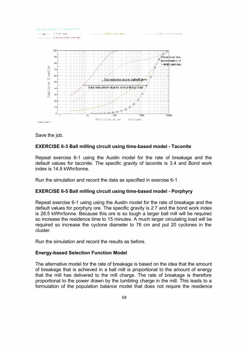
7/14/2019 modsim


68

Save the job.

EXERCISE 6-3 Ball milling circuit using time-based model - Taconite

Repeat exercise 6-1 using the Austin model for the rate of breakage and thedefault values for taconite. The specific gravity of taconite is 3.4 and Bond workindex is 14.9 kWhr/tonne.

Run the simulation and record the data as specified in exercise 6-1.

EXERCISE 6-5 Ball milling circuit using time-based model - Porphyry

Repeat exercise 6-1 using using the Austin model for the rate of breakage and thedefault values for porphyry ore. The specific gravity is 2.7 and the bond work indexis 28.5 kWhr/tonne. Because this ore is so tough a larger ball mill will be requiredso increase the residence time to 15 minutes. A much larger circulating load will berequired so increase the cyclone diameter to 76 cm and put 20 cyclones in thecluster.

Run the simulation and record the results as before.

Energy-based Selection Function Model

The alternative model for the rate of breakage is based on the idea that the amountof breakage that is achieved in a ball mill is proportional to the amount of energythat the mill has delivered to the mill charge. The rate of breakage is thereforeproportional to the power drawn by the tumbling charge in the mill. This leads to aformulation of the population balance model that does not require the residence

7/14/2019 modsim


69

time of the solids in the mill to be specified as the primary capacity parameter. It isnecessary only to specify the net power drawn by the mill.

The variation of the selection function with particle size is usually modeled using aslightly different relationship to that used by Austin. The alternative model is used

in exercise 6-2 which illustrates the use of the closed circuit ball mill to grindlimestone.

Exercise 6-4 illustrates the model when applied to the grinding of taconite andexercise 6-6 illustrates its application to the tough porphyry ore.

Exercise 6-2 Ball mill circuit - Energy-based model for Limestone

This exercise uses the flowsheet that was constructed in exercise 6-1.

Open the job that was saved in exercise 6-1.

All data remains the same except that the ball mill will be modeled using theHerbst-Furstenau energy-specific model for the rate of breakage. Use MODSIMmodel HFMI. The parameters for the selection have these values S1E = 1.15tonnes/kWhr, zeta1 = 0.185 and zeta 2 = -0.100 (Note the negative value which isessential). Breakage function values are Beta = 3.723, gamma = 0.748, delta = 0.0and Phi 5 = 0.720.

Note that the Herbst-Furstenau model requires the power input to the mill and notthe average residence time. Set the power to the estimate power obtained inexercise 6-1 (1.07 MW)

Run the simulation and record the data as in exercise 6-1 and compara the datafrom the two exercises.

Exercise 6-4 Ball mill circuit - Energy-based model for Taconite

Repeat exercise 6-2 using the Herbst-fuerstenau model. Use the power that wascalculated in exercise 6-3 (2.34 MW).

Selection function parameters for this ore are:

S1E = 0.75 tonnes/kWhr

zeta1 = 0.23

zeta2 = -0.2(Note the negative value)

Breakage function parameters are:










7/14/2019 modsim


70

beta = 3.723

gamma = 0.624

delta = 0

Phi5 = 0.65

Exercise 6-6 Ball mill circuit - Energy-based model for porphyry

Repeat exercise 6-5 using the Herbst-fuerstenau model. Use the power that wascalculated in exercise 6-5 (1.48 MW).

Selection function parameters for this ore are:

S1E = 0.3 tonnes/kWhr

zeta1 = 0.3

zeta2 = -0.25

Breakage function parameters are:

beta = 3.723

gamma = 0.748

delta = 0

Phi5 = 0.72

This exercise provides a good opportunity to observe the behavior of the circuitprocessing this ore as the power input to the mill varies. Run the simulation severaltimes varying the power input in steps from 3000 kW down to 1300 kW. Plot thecirculating load as a function of the power and observe the size distribution graphsat each power level. This will give you a good idea how to interpret the four sizedistribution graphs as the mill handles less and less of the comminution load.

MODULE 7 Liberation

A liberation model for comminution operations can be used effectively when themodel is based on the Population Balance approach. Two such models have beenimplemented in Modsim. The "ljubljana" model and the "beta function model". Bothmodels describe the internal structure of the bivariate breakage function, a.k.a. the

7/14/2019 modsim


71

Andrews-Mika diagram. The ljubljana model is a clever conceptual model of the A-M diagram. Its main advantage is that it contains a single parameter that can bechanged to describe a wide range of textures, and therefore simulate the liberationprocess. The beta function model on the other hand is based on carefulobservation of the liberation process in real ores. It contains a number of

parameters that can be adjusted to provide an as accurate as possible descriptionof the liberation process under almost all circumstances, including differential andpreferential breakage. Both models are currently two-phase models, and onephase is invariably the gangue phase while the other is the phase of interest, thevaluable. Although this may be seen as a limitation, it represents a tremendousimprovement over assuming that liberation remains constant in comminutioncircuits.

Simulation of liberation is quite a complex subject. However, and fortunately, theinterface implemented in MODSIM greatly facilitates the effective use of this rather advanced technology.

The details of the modeling of simulation and comminution can be found in Chapter 3 of the textbook and in Technical Notes 10

Objectives

1. Learn how to specify liberation data for a binary ore feed stream in MODSIM.

2. Learn how to simulate the liberation process together with the size reductionprocess in a Ball Mill using a liberation model.

3. Learn to view and interpret liberation simulation results.

This module contains a single section:

Simulation of a closed continuous grinding circuit with concentration andclassification of a Taconite ore.

Simulation of a closed continuous grinding circuit with concentration andclassification of a Taconite ore.

Taconite is an iron ore containing mainly Chert and Iron Oxides. In this case theore is not supergenic, and the iron oxides are represented almost exclusively byMagnetite. The texture of the ore is rather complex, and liberation is fundamentallyimportant for this operation to be economic.

The liberation of magnetite in the plant that is to be studied in this module isdescribed in Section 10.6 of the textbook.

Flowsheet

http://www.mineraltech.com/MODSIM/ModsimTraining/Module7/TechnicalNotes-10-Liberation.pdf



http://www.mineraltech.com/MODSIM/ModsimTraining/Module7/module7-toptframe.html



http://www.mineraltech.com/MODSIM/ModsimTraining/Module7/module7-toptframe.html#anchor381688






7/14/2019 modsim


72

System Data

Unit Model Parameters Simulation Results Exercises

Flowsheet

The grinding circuit to be studied here is a simplified version of a real Taconitegrinding/concentration operation. The flowsheet is described here. Your first task isto draw this flowsheet in MODSIM. Save your job when done.

System Data

When simulating a grinding circuit with liberation, additional information is requiredabout the ore:

1. the ore's liberation spectra, i.e. the distribution of particle grades at several sizeranges is required. This describes the liberation state of the ore as it enters thecircuit.

2. the ore's textural parameters. This describes how the liberation spectra changesas the ore is ground.

Click here to see the complete system data specification for this simulation. Enter this system data in Modsim. Save your job at this stage.

Unit model parameters

As usual we need to enter model parameters for each unit in the simulation. Clickhere to see a set of parameters that work with this simulation. Pay special attentionto the Ball Mill model.

Simulation results

After running this simulation, it is possible to view one of the Andrews-Mikadiagrams that was generated by the Ljubljana model. More importantly, you shouldbe able to review the liberation distributions in the circuit streams, and understandwhat the grade distributions mean.

1. View the Andrews-Mika diagram 2. Liberation spectra around the Ball Mill 3. Liberation spectra around the Wet Magnetic Drum

4. Liberation Spectra around the Hydrocyclone









http://www.mineraltech.com/MODSIM/ModsimTraining/Module7/flowsheetdesc.html



http://www.mineraltech.com/MODSIM/ModsimTraining/Module7/systemdatadesc.html


http://www.mineraltech.com/MODSIM/ModsimTraining/Module7/unitmodelparam.html


http://www.mineraltech.com/MODSIM/ModsimTraining/Module7/ViewingAM.html


http://www.mineraltech.com/MODSIM/ModsimTraining/Module7/ViewingBMDlib.html


http://www.mineraltech.com/MODSIM/ModsimTraining/Module7/ViewingWMDlib.html


http://www.mineraltech.com/MODSIM/ModsimTraining/Module7/ViewingHClib.html













7/14/2019 modsim


73

Exercises

Two simple exercises are to be attempted in this module:

1. Exercise 7-1

2. Exercise 7-2

Flowsheet Description

The circuit grinds Taconite that has been pre-concentrated in a Cobber MagneticDrum, thus the feed stream is labeled Cobber Conc. For those unfamiliar with thisprocess, a Cobber is basically a high-intensity magnetic drum separator, designedto operate with relatively coarse ore particles. The Cobber Concentrate enters thecircuit through a sump, which regulates the flow and solids content to the feed to aBall Mill. Different than a standard closed grinding circuit with classification, this

circuit contains a concentrating stage between the milling and classification stages.This concentration is accomplished by a bank of Wet Magnetic Drums, treating theBall Mill Discharge. The solids content in the feed to the drum must also beregulated by a sump, since the Ball Mill discharge solids content is too high for thisprocess. The tailings of the Magnetic Drum are discarded. This makes a lot of sense since regrinding particles that contain little or no Iron is definitely not costeffective. The magnetic drum concentrate is fed to a hydrocyclone classifier cluster, through a sump, again to regulate the solids content. The hydrocyclone

http://www.mineraltech.com/MODSIM/ModsimTraining/Module7/exercise7-1.html






7/14/2019 modsim


74

underflow is recirculated, with the circuit feed, back to the mill. The overflow streamis the product of the grinding circuit, and this undergoes further concentration andscreening.

Note: when drawing the magnetic drum icon you will have to reflect the icon if you

want your flowsheet to look similar to the one in the figure. Also, if you would like tosee this flowsheet being drawn you can use your ScreenCam Player that wasinstalled with your Modsim, CD ROM version 3.2. Just run scplayer from your Programs -> ModsimV32 Student shortcuts.Click on the upper-left icon on theScreenCam player window frame and choose File Open... Load the Mod7-

A1drawing-smallfairlane.scm file from the Course directory in the Modsiminstallation directory. Push Play. Unfortunately, ScreenCam files are too large todeliver over the internet, and we have abandoned this tool in favor of viewlets.

System Data

Ore Characteristics

The ore contains two phases, namely Chert and Magnetite. Phase densities are2.76 and 5.38 g/cc respectively. The maximum particle size is about 10 mm in theCobber Concentrate and 25 sizes are more than enough. Set the number of gradeclasses to 12 and make sure that you are specifying specific gravities by Mineral.

7/14/2019 modsim


75

Click on Set up grade classes. Modsim automatically sets up 10 equally spacedgrade classes and the two liberated ends. This is the standard setup for liberation

data, and liberation is normally measured using these same grade classes whenimage analysis techniques are employed. Note that the densities of each of the 12particle types are correctly calculated by Modsim.

At this stage, you should go ahead and set up the liberation model data, so click onthe Specify liberation model data button. For this simulation we are going to use

7/14/2019 modsim


76

the Ljubljana model. Set the parameter to 50 and check the Calculate Andrews-Mika diagram check box.

Accept these parameters and then accept the specified particle types.

Feed stream data

We now need to specify the characteristics of the feed stream. Double-click on thefeed stream number. For the size distribution you can use a Rosin-Rammler distribution with D63.2 = 1.4 mm and Lambda = 1.2, and 20 size classes. The feedrate is about 300 tonnes/hour and the solids content is about 70% in the Cobber Concentrate.

Normally, system data is complete at this stage when there is no liberation dataavailable. In this case, the complete liberation spectra has been measured for theCobber Concentrate stream. Click on Specify grade distributions.

Specifying grade distributions by hand demands time and is error prone.Fortunately, the liberation spectra can be imported from a file. Click on Import datafrom file, and browse your way to the DemoJobs directory in your Modsim

7/14/2019 modsim


77

installation directory. Double click on the LiberationData folder and select thecobcon.dat file. Click on Open.

Click on the differentSize range

radio buttons to see the particle gradedistributions that are associated with each size. This is the liberation spectra for asingle stream and this data was measured by Image Analysis on a sample takenfrom the real plant. To see how this data looks like in a 3D chart, click here.

Cobber Concentrate Liberation Spectra

http://www.mineraltech.com/MODSIM/ModsimTraining/Module7/CobberConcentrate.html




7/14/2019 modsim


78

This is a conditional, on size, grade distribution. Liberation was measured in 11size ranges. All particles in the same size range are identified by an unique color.The distributuion is called conditional on size because each size adds up to 100%,i.e. there is no size distribution information associated to these numbers, and onlythe liberation characteristics at each size is shown. There are 12 particle types.

Grade 0 represents pure Chert and grade class 100 represents pure Magnetite.Notice how particles above 355 microns are completely unliberated in thispopulation. Also, notice the transition between unliberated and mostly liberated inthe range 355 x 75 microns. We could say that the liberation size for this ore isabout 106 microns, because bellow 106 microns we can separate Chert and lowgrade particles from Magnetite and high grade particles.

Note: This data was measured by Image Analysis of particles sampled in the realplant. There is quite a lot of controversy in the literature about liberationmeasurement. One of the reasons for this controversy is that even experiencedresearchers confuse the three fundamental liberation problems: measurement,prediction and simulation. In the keynote address to the Australian Comminution 98conference, Dr. King decided to put a lecture together aimed at clearly definingthese problems and thus putting an end to this confusion (hopefully). This keynoteaddress was included with the student version of Modsim. If you are interested inliberation, you should view this presentation. Just double-click in thekeynoteAudio.exe file in the Course folder contained in your Modsim installationfolder. PDF files related to the keynote address are also included in this folder.

Accept this grade distribution and then accept the feed stream data.

Water addition streams data

Double-click on the water streams to specify water rates. All water streams in this job are specified by the percentage of solids in the Sump units. In this way,Modsim calculates how much water is needed so that the desired solids content isachieved. Specify 77% solids in the Ball Mill Feed sump, 50% solids in theMagnetic Drum Feed sump and 57% solids in the Hydrocyclone Feed sump. It isalso a goog idea to add names to the water addition streams.

Closing remarks

No other system data is required but it would be nice to have all internal streamsnamed as well. Click on Accept. You will see the following Notice window.

7/14/2019 modsim


79

This is because we checked the "Calculate Andrews-Mika diagram for Ljubljanamodel on exit" when specifying the Liberation model. Modsim calculates several

Andrews-Mika diagrams, one for each particle type specified, using the singlemodel parameter PhiA. You will be able to see one of these Andrews-Mikadiagrams once you completed the simulation.

Unit model parameters

Ball Mill Wet Drum magnetic Separator Hydrocyclone

Ball Mill

Choose model GMIL.

residence time = 4 minutes

Selection function: Taconite

Liberation model: Ljubljana model

Note: This model has a set of pre-determined Selection and Breakage functions. Itis necessary to tell Modsim that the Ljubljana model is to be used. This is becausethe Beta function model cannot be pre-calculated in the same fashion as theLjubljana model, and it depends on the Breakage function parameters specified inthe mill model. This is so because the Beta function model allows for preferential

breakage, and the solution is constrained by the traditional breakage function andthe principle of conservation of phase. If you are interested in phenomena such asdifferential breakage, preferential breakage, selective breakage, and the Andrews-Mika itself, read this technical paper on Mineral Liberation and the BatchComminution Equation.

Here the particle size distribution in the mill product is calculated using thetraditional PBM approach. The selection function is used to determine theprobability a particle of a given size breaks (independent of its composition) andthe breakage function is used to calculate the probability that a progeny reports toa given size below that of the parent particle size. The Andrews-Mika is used to

determine the probability that the progeny reports to any one of the twelve gradeclasses that have been defined, and this of course depends on the parentcomposition, and how much smaller than the parent the progeny is. Here is adescription of an Andrews-Mika diagram and this should help you understand therole of this important function when liberation is involved. The conception of theLjubljana model has been published in ths technical paper on Calculation of theLiberation Spectrum in Products Produced in Continuous Milling Circuits.

http://www.mineraltech.com/MODSIM/ModsimTraining/Module7/unitmodelparam.html#anchor506335






http://www.mineraltech.com/MODSIM/ModsimTraining/Module7/MinLib.pdf



http://www.mineraltech.com/MODSIM/ModsimTraining/Module7/AMmodel.html


http://www.mineraltech.com/MODSIM/ModsimTraining/Module7/ljubljana.pdf











7/14/2019 modsim


80

Wet Drum Magnetic Separator

Choose model WDM2

Sharpness index = 0.9

Grade for 50% recovery = 0.1

Small size limit of short circuit = 0.466

Bypass coefficient = 56

Water Split to tail stream = 0.78

The magnetic separator is largely dependent on grade, and grade is indeed theoperating variable in this separation model. Particles with as little as 10%Magnetite have a 50% probability of being recovered in the magnetics stream. Lowgrade particles cannot be economically ground and these are removed from thecircuit.

Hydrocyclone

Choose model CYCA

Short circuit to underflow = 0.1


Cut size = 120 microns

Classification function = Logistic

Allow D50 to vary with density and specify the parameter for D50 x density as 0.8

This is a simple model for the Hydrocyclone. In the plant, it was observed thatparticles with high Magnetite content tend to concentrate in the Underflow. This is

because D50 is smaller for havier particles, as previuosly discussed in the course.

Ball Mill

Choose model GMIL.

residence time = 4 minutes

7/14/2019 modsim


81

Selection function: Taconite

Liberation model: Ljubljana model

Note: This model has a set of pre-determined Selection and Breakage functions. It

is necessary to tell Modsim that the Ljubljana model is to be used. This is becausethe Beta function model cannot be pre-calculated in the same fashion as theLjubljana model, and it depends on the Breakage function parameters specified inthe mill model. This is so because the Beta function model allows for preferentialbreakage, and the solution is constrained by the traditional breakage function andthe principle of conservation of phase. If you are interested in phenomena such asdifferential breakage, preferential breakage, selective breakage, and the Andrews-Mika itself, read this technical paper on Mineral Liberation and the BatchComminution Equation.

Here the particle size distribution in the mill product is calculated using the

traditional PBM approach. The selection function is used to determine theprobability a particle of a given size breaks (independent of its composition) andthe breakage function is used to calculate the probability that a progeny reports toa given size below that of the parent particle size. The Andrews-Mika is used todetermine the probability that the progeny reports to any one of the twelve gradeclasses that have been defined, and this of course depends on the parentcomposition, and how much smaller than the parent the progeny is. Here is adescription of an Andrews-Mika diagram and this should help you understand therole of this important function when liberation is involved. The conception of theLjubljana model has been published in ths technical paper on Calculation of theLiberation Spectrum in Products Produced in Continuous Milling Circuits.


Choose model WDM2






The magnetic separator is largely dependent on grade, and grade is indeed theoperating variable in this separation model. Particles with as little as 10%














7/14/2019 modsim


82

Magnetite have a 50% probability of being recovered in the magnetics stream. Lowgrade particles cannot be economically ground and these are removed from thecircuit.

Hydrocyclone

Choose model CYCA






This is a simple model for the Hydrocyclone. In the plant, it was observed thatparticles with high Magnetite content tend to concentrate in the Underflow. This isbecause D50 is smaller for havier particles, as previuosly discussed in the course.


Choose model WDM2






The magnetic separator is largely dependent on grade, and grade is indeed theoperating variable in this separation model. Particles with as little as 10%

Magnetite have a 50% probability of being recovered in the magnetics stream. Lowgrade particles cannot be economically ground and these are removed from thecircuit.

Hydrocyclone

Choose model CYCA

7/14/2019 modsim


83







Hydrocyclone

Choose model CYCA







View the A-M diagram

There are in fact 300 A-M diagrams that are generated by the Ljubljana model for this simulation, one for each particle type, 12 grade classes x 25 size classes. Tosee one of the A-M diagrams generated by the Ljubljana model, select View ->Flowsheet. Right-click on the ball mill icon and select Andrews-Mika diagram. Take

some time analysing the diagram. Make a note of the liberation size, i.e. the size atwhich liberated particles start appearing from breakage of a parent particle of about45% Magnetite. Note the ratio between parent size and liberation size. You maywant to run this simulation at several values of phiA and compare the diagramsthat are generated. remember tha phiA is the parameter that is defined by thetexture of the ore.

Liberation spectra around the ball mill

7/14/2019 modsim


84

To view the liberation spectra in the ball mill streams select View->Liberationdistribution graphs. The Plot liberation distribution s form is opened. This workssimilarly to the size distribution interface.

Double-click on the streams you want liberation spectrum to be displayed. Thestream numbers are added to the Graph list. In this case we want to view the ball

mill feed and discharge streams. Click on view graph.

7/14/2019 modsim


85

For each stream, the line represents the distribution of particle grades over all sizeranges. The ball mill feed stream has no liberated chert particles and smallamounts of low grade particles. It also shows that most particles are accumulatingin the 30 to 50% Magnetite grade range. Also, about 9% of liberated Magnetiteparticles is present in the mill feed. This leads to an important and fundamentalquestion: Do we want to further grind liberated Magnetite? The ball mill dischargeon the other hand contains about 17% liberated Chert particles and 21% liberatedMagnetite particles, and the unliberated particles are spread more uniformely over the grade domain. The mill is indeed doing its job!

Note: Why are there so few particles of low grade in the ball mill feed? See the

liberation distributions around the Wet magnetic Drum.

Liberation spectra around the Wet Magnetic Drum

Now select the Wet Magnetic Drum feed (ball mill discharge), concentrate andtailings streams. Clear the ball mill feed stream if this is still selected. Click on viewgraph.

7/14/2019 modsim


86

The feed stream is the ball mill discharge. We have already discussed this in theprevious section. The tailings stream is made up of almost 50% of liberated Chertparticles, and an accumulation of low grade particles. It also contains about 7% of liberated magnetite particles. In the actual plant, this stream is treated in ascavenging unit, and the liberated Magnetite is recovered. Their presence in thetailings stream is due to the by-pass factor in the Drum. The concentrate streamcontains no liberated Chert particles. That is the reason the ball mill feed does notcontain this type of particles. From about 30% Magnetite content and up, the Drumrecovers most particles, which is expected. The concentrate stream contains about27% liberated Magnetite particles.

Liberation spectra around the Hydrocyclone

Now select the Hydrocyclone streams. Click on view graph.

7/14/2019 modsim


87

The underflow contains mostly particles in the 30 to 50% Magnetite grade range.However, it also contains significant amounts of liberated and high grade Magnetiteparticles, even though most of these particles are in the smaller size ranges. Thisis a good indication of the concentrating action in the Hydrocyclone. These smallhigh grade particles are redirected to the mill. Surely, we would rather regrind onlythe unliberated particles, but this inherent Hydrocyclone concentrating action isdifficult to avoid.

Exercise 7-1

Complete the simulation described in the section above. Make a note of the

recovery and grade of Magnetite in the cyclone overflow stream.

Exercise 7-2

Ore bodies are not homogeneous and variability in grade, texture and other properties is in fact the norm. The Taconite studied in this module has a texturecharacterized by the parameter phiA in the Ljubljana model. Taconite from different

7/14/2019 modsim


88

areas in the ore body may be different in texture. Consider the hypothetical casesbelow:

In the images above, Chert is dull grey while Magnetite is bright. Note how thetexture parameter is directly related to the complexity of texture, in themorphological sense. In the left particle, texture is so complex that grain sizebecomes a concept that is difficult to grasp. Interphase area per unit volume of phase is the quantitative property that applies in all cases, and this is how theparameter phiA is derived.

Run simulations using the values of phiA in the Table above. Compare grade andrecovery of Magnetite for each case in the Cyclone Overflow stream. (You alreadycompleted the simulation for PhiA = 50 in the previous exercise.)

MODULE 8 Assessment of Existing Plants and Model Calibration

Once a simulator such as MODSIM has been mastered, the simulation of evencomplex plants becomes a straightforward task. It is a matter of specifying theflowsheet, choosing suitable models for the unit operations and characterising thefeed material. The real difficulty with the method lies in the choice of parametersand settings for the unt models. In most cases these values do not have absolutevalues and they must be chosen to suit the characteristics of the particular materialthat is to be processed in a particular plant or installation . Usually the parametershave values that are strongly influenced by the material that is to be processed, soparameters parameter values must be obtained for every project. Parameters for

the models can be obtained from data collected in the laboratory or from data thatis collected on an operating plant. Clearly the second alternative is not available if the plant does not yet exist. A number of standard laboratory methods have beendeveloped to measure the parameters for many of the models and one of these willbe discussed later in the course. We will concentrate in this module on methodsthat can be used to obtain model parameter values from operating plant data andon the interpretation of these values in terms of plant performance.

7/14/2019 modsim


89

OBJECTIVES OF THIS MODULE

1. Learn to use the features in MODSIM that can be used to compare simulationoutput with real data.

2. Learn to interpret parameter values in terms of the operating characteristics of the units and to diagnose operating problems.

3. Learn how to use simulation to achieve better plant operation.

Two examples are included in this module. The first examines an existingconventional grinding circuit and the second an existing milling circuit that hasspecific mineral liberation characteristics.

Determining Parameters from Operating Data

When good data are available from a plant sampling campaign, the operatingvalues of the parameters in the models for the unit operations can be estimatedusing conventional parameter estimation techniques. Typically plant streams aresampled and analysed and, if the feed and product streams from any particular unitare available, the parameters for that unit can be estimated using the MODSIMmodel directly. All MODSIM models accept the details of the unit feed as input andproduce the simulated output of that unit. When experimental data are available for the feed and product streams, the least-squares best estimates of the unitparameters can be obtained by matching the simulated output to the measuredoutput to minimize the sum of squared deviations. This is best done by embeddingthe code for the unit model as it is used in MODSIM into a least-squaresminimization search program. This method is very effective and usually producesgood estimates of the parameters for the unit in question. Sometimes data that arespecific to the material inside the unit must also be used to estimate all theparameters for that unit. The size distribution in the load of a ball or SAG mill is anexample when it is necessary to estimate the parameters that define theclassification action of the grate discharge. Data of this sort are typically difficult toget and it is often necessary to use best guess values for these parameters.

When operating data are not available for all the process streams that areassociated with a particular unit, data from a larger section of the plant must beused. This can be done by embedding the entire Modsim simulator inside a leastsquares minimization program. Typically, measured size distributions from severalof the plant streams are matched against the simulator outputs for those streams.Modern optimization codes make this possible and the method is now usedroutinely.

Exercise 8-1 illustrates this method.

Exercise 8-1 Assessment of a rod and ball mill circuit.

http://www.mineraltech.com/MODSIM/ModsimTraining/Module8/FrmDetermineParameters.html


http://www.mineraltech.com/MODSIM/ModsimTraining/Module8/FrmMineralLiberation.html







7/14/2019 modsim


90

The data given in the spreadsheet resulted from a careful sampling campaign onan operating plant. The spreadsheet can be viewed by clicking here.

In particular, both feed and product streams were sampled for the rod and ballmills. These data were used to estimate the breakage and selection function

parameters for both of these mills. In each case the average residence time of thesolids in the mill was estimated from the mill dimensions, the media load and theestimated flowrate through the mill. The values found for the residence times were3.40 minutes in the rod mill and 2.19 minutes in the ball mill. The simple perfectlymixed mill model MILL in MODSIM was used for the ball mill and the model RODMwas used for the rod mill. The least-squares best estimates of the parameters aregiven in Tables 1 and 2. Since the size distrinbution in the cyclone feed was notmeasured during the sampling campaign, the parameters for the cyclone could notbe estimated directly.

Table 1 Estimated parameters for the rod mill.

Selection function Breakage function

S1 = 1.658 1/min beta = 3.696

alpha = 0.602 gamma = 1.481

mu = 1.4 mm delta = 0.0

Lambda = 0.736 Phi = 0.242

Table 2 Estimated parameters for the ball mill.

Selection function Breakage function

S1 = 1.508 1/min beta = 7.699 alpha = 1.662 gamma = 0.683

mu 1.4 delta = 0.0

Lambda = 0.735 Phi = 0.683

These values can be tested in the simulation and the calculated size distributionscan be compared to those measured during the plant sampling campaign. Thecomparison is facilitated in MODSIM since the measured data can be entered aspart of the system data. The measured data are entered using the system dataform. Double click on each stream for which measured size distribution data are

available and enter the experimental data in the usual way. It is a good idea tospecify a name for the stream at the same time. The information that is entered inthis way is not used by MODSIM for simulation calculations in any way. It is merelydisplayed in the graphs for comparison.

The physical dimensions of the hydrocyclones were specified in the data set andunder normal opertaing conditions no other infromation is required to specify theoperation of the hydrocyclones if the Plitt model is used. The feed head was



http://www.mineraltech.com/MODSIM/ModsimTraining/Module8/Exercise8-1Wks.htm





7/14/2019 modsim


91

estimated to be 3.81 m. However in practice the cyclones should be calibrated tomatch the actual operation. Three calibration factors are provided in the model for this purpose. It is a simple matter to adjust these using least-squares stimation tofind a good fit to the experimental size distributions. In this case the factors foundwere for D50c, 0.293, for the sharpness index 0.152 and fo rthe flow split 0.856.

The resulting simulated output for this plant is shown in Figure 1.

Figure 1 Simulator output for the plant as sampled. Points are experimental dataand lines are the simulator output.

It should be immediately obvious that the simulation is a good representation of theactual plant operation since the size distributions match the experimental data well.However, this is an example of a poorly operating milling circuit. Note how the rodmill is accounting for the greatest portion of the size reduction. The ball mill is notproducing as much size reduction as it could if the circuit were set up moreappropriately.

Some unusual aspects of this data are apparent. The media for the ball mill aredescribed as slugs rather than balls. This means that the media are not sphericalbut have flat surfaces which have the effect of cushioning the very fine particles.

This shows up as an unusually high value for alpha (1.662) in the selection functionfor the ball mill. This makes the specific rate of breakage fall off rapidly as the sizedeceases. This can be seen by inspecting the selection function for the ball mill. (Right click the mill icon when viewing the flowsheet). In this case this leads toinefficient grinding in the ball mill.

Both the spigot and vortex finder diameters are unususally large in this plant. Thisgives rise to an unusually large cut point for the size of cyclone that is used.

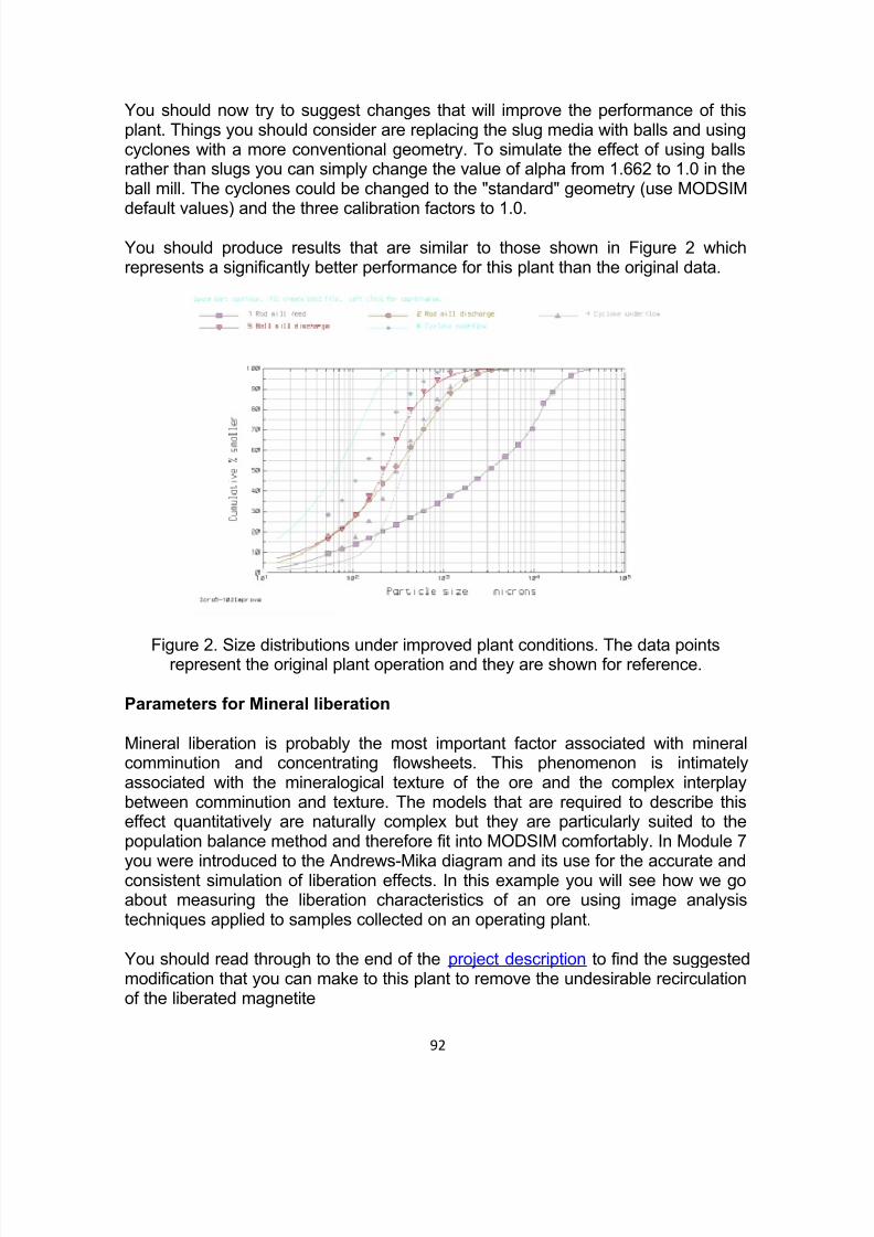
7/14/2019 modsim


92

You should now try to suggest changes that will improve the performance of thisplant. Things you should consider are replacing the slug media with balls and usingcyclones with a more conventional geometry. To simulate the effect of using ballsrather than slugs you can simply change the value of alpha from 1.662 to 1.0 in theball mill. The cyclones could be changed to the "standard" geometry (use MODSIM

default values) and the three calibration factors to 1.0.

You should produce results that are similar to those shown in Figure 2 whichrepresents a significantly better performance for this plant than the original data.

Figure 2. Size distributions under improved plant conditions. The data pointsrepresent the original plant operation and they are shown for reference.

Parameters for Mineral liberation

Mineral liberation is probably the most important factor associated with mineralcomminution and concentrating flowsheets. This phenomenon is intimatelyassociated with the mineralogical texture of the ore and the complex interplaybetween comminution and texture. The models that are required to describe thiseffect quantitatively are naturally complex but they are particularly suited to thepopulation balance method and therefore fit into MODSIM comfortably. In Module 7

you were introduced to the Andrews-Mika diagram and its use for the accurate andconsistent simulation of liberation effects. In this example you will see how we goabout measuring the liberation characteristics of an ore using image analysistechniques applied to samples collected on an operating plant.

You should read through to the end of the project description to find the suggestedmodification that you can make to this plant to remove the undesirable recirculationof the liberated magnetite

http://www.mineraltech.com/MODSIM/ModsimTraining/Module8/Module8data.pdf




7/14/2019 modsim


93

MODULE 9

OWN FLOWSHEETS

This module has been set aside for participants to investigate any flowsheet/s that

is/are of particular interest.

We encourage you to look around for some interesting flowsheet and start toinvestigate what data would be required to achieve a successful simulation. It isusually possible to get started using defaults that are supplied by MODSIM but it isessential to learn to be sensitive to the effect of assumptions on a simulationoutput. Another important aspect of trying to simulate unusual flowsheets is theavailability of suitable models for all the unit operations that are involved. We willnever have enough models. New equipment is being invented and tried continuallyand model development inevitably lags behind. Reliable models are not easy todevelop and this can be done successfully only when good experimental data are

available.

Another issue that is topical in this group is the provision of basic simple models inMODSIM for preliminary simulations. We remain unconvinced that this is a goodidea. This is an opportunity to find some examples to show the utility of thisapproach.

We encourage you to post any interesting flowsheets on the bulletin board and wewill make suggestions about the best way to simulate them and also try to identifythe critical elements and data. Remember that you can pack incomplete jobs sothat even if you have no data it may be worth packing a job that consists only of the

flowsheet and attaching it to a bulletin.

Module 10: Investigating Mineral Processing in a VirtualLaboratory

All of the simulations that you have done up to now require the specifications of parameters for the models that are used to simulate the units that make up theflowsheet. These parameters define the operation of the units for the application onhand and they usually vary with the ore that is to be processed. It is important toobtain good values for these parameters if the simulation is to be realistic. Thereare three techniques that are commonly used to obtain estimates of theparameters: sampling a plant that is currently in operation, by generating data from

samples taken during careful laboratory experiments and finally using accumulateddata banks of parameter values from previous successful simulation studies. Of these, the first method provides the most reliable data but is usually the mostdifficult method to use because of the difficulties inherent in obtaining goodconsistent samples from a large operating plant. In most cases a pilot plant shouldbe used if this is available. The third method is the most commonly used approachbut it does require access to good operating databases. The second method using

7/14/2019 modsim


laboratory experimentation can be very effective and it is the subject of thismodule. It is important to plan and execute a laboratory experiment properly in order toensure that it does yield good information about the model that is being tested. Wewill use one of the newest education techniques, the virtual laboratory, to

investigate a common laboratory experiment that is often used to measure specificrate of breakage in a ball mill. If you work through this experiment, you will learnthe technique and also how to interpret the data that are obtained in the laboratory. The virtual laboratory has been designed to allow you to undertake a virtualexperiment that is a close replica of the actual experiment and to gather data thatare closely similar to data that are obtained in a well-conducted real experiment inthe laboratory. Objectives for this module. You will learn the standard procedure for conducting one of the experiments thatare normally used to measure parameters for the ball mill model. You will learn how to analyze the data and to extract values of model paramentersthat can be used for simulation purposes.

A brief description of the experiment is given here. You must install the Virtual Laboratory software on your computer in order to dothe experiment. You can download the Virtual Laboratory setup program from here. The file is SETUPVLab.EXE which you should run when the download iscomplete. Like MODSIM this program can be uninstalled if you do not wish to keepit on your machine. The experimental procedure is described here.

http://www.mineraltech.com/MODSIM/ModsimTraining/Module10/BatchBallMillExperiment.htm



http://www.mineraltech.com/mete6010/Module10/SETUPVLab.EXE


http://www.mineraltech.com/MODSIM/ModsimTraining/Module10/ExperimentalProcedure.htm






modsim

Documents