Barba‑Montoya et al. BMC Ecol Evo (2021) 21:83 https://doi.org/10.1186/s12862‑021‑01798‑6

RESEARCH ARTICLE

Molecular and morphological clocks for estimating evolutionary divergence timesJose Barba‑Montoya1,2, Qiqing Tao1,2 and Sudhir Kumar1,2,3*

Abstract

Background: Matrices of morphological characters are frequently used for dating species divergence times in sys‑tematics. In some studies, morphological and molecular character data from living taxa are combined, whereas others use morphological characters from extinct taxa as well. We investigated whether morphological data produce time estimates that are concordant with molecular data. If true, it will justify the use of morphological characters alongside molecular data in divergence time inference.

Results: We systematically analyzed three empirical datasets from different species groups to test the concordance of species divergence dates inferred using molecular and discrete morphological data from extant taxa as test cases. We found a high correlation between their divergence time estimates, despite a poor linear relationship between branch lengths for morphological and molecular data mapped onto the same phylogeny. This was because node‑to‑tip distances showed a much higher correlation than branch lengths due to an averaging effect over multiple branches. We found that nodes with a large number of taxa often benefit from such averaging. However, considerable discordance between time estimates from molecules and morphology may still occur as some intermediate nodes may show large time differences between these two types of data.

Conclusions: Our findings suggest that node‑ and tip‑calibration approaches may be better suited for nodes with many taxa. Nevertheless, we highlight the importance of evaluating the concordance of intrinsic time structure in morphological and molecular data before any dating analysis using combined datasets.

Keywords: Species divergence time estimation, Molecular clock, Morphological clock, Fossil calibration, Bayesian inference

© The Author(s) 2021. Open Access This article is licensed under a Creative Commons Attribution 4.0 International License, which permits use, sharing, adaptation, distribution and reproduction in any medium or format, as long as you give appropriate credit to the original author(s) and the source, provide a link to the Creative Commons licence, and indicate if changes were made. The images or other third party material in this article are included in the article’s Creative Commons licence, unless indicated otherwise in a credit line to the material. If material is not included in the article’s Creative Commons licence and your intended use is not permitted by statutory regulation or exceeds the permitted use, you will need to obtain permission directly from the copyright holder. To view a copy of this licence, visit http:// creat iveco mmons. org/ licen ses/ by/4. 0/. The Creative Commons Public Domain Dedication waiver (http:// creat iveco mmons. org/ publi cdoma in/ zero/1. 0/) applies to the data made available in this article, unless otherwise stated in a credit line to the data.

BackgroundThere is a growing interest in using morphological data to infer species divergence times in systematics by using it in morphological clock analyses (e.g., [1–8]) or combining it with molecular data in total-evidence dat-ing approaches (e.g., [9–14]). In total-evidence dating, morphological characters from dated fossil species and extant species are analyzed along with molecular data under character-specific models of morphological and

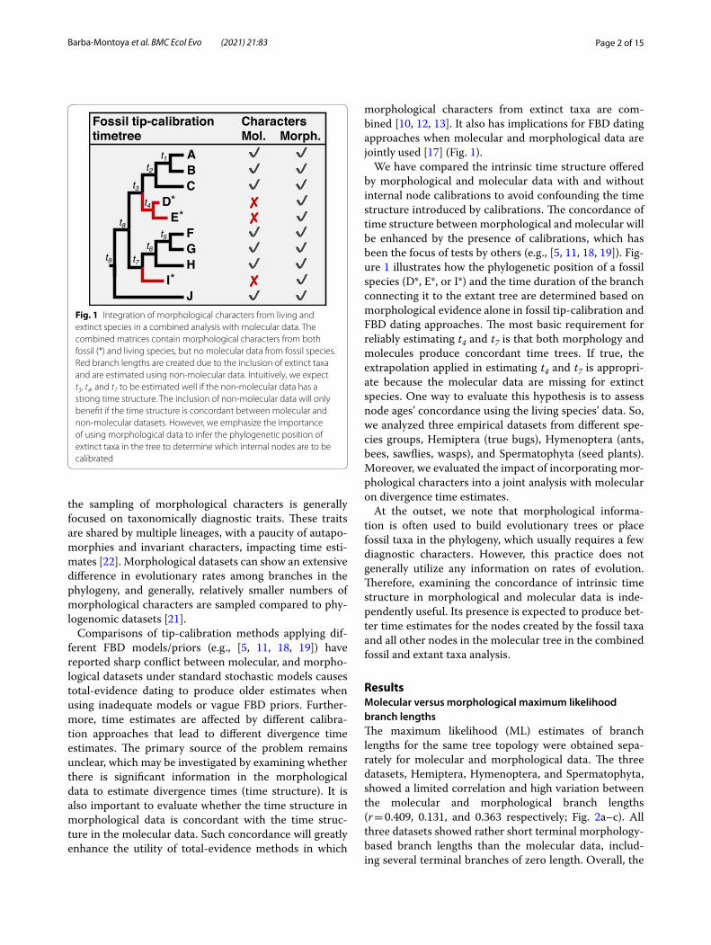
molecular evolution (e.g., [10, 15]). Tip-calibrations are typically used as constraints on the timing of lineage divergence by including dated fossil species in the relaxed clock analyses [16] (Fig.  1). Moreover, in the fossilized birth–death (FBD) process [17, 18], the fossil species’ age provides the calibration information that translates the morphological distances into absolute times and rates, which are propagated to the other nodes on the phylogeny.

Nevertheless, utilizing morphological characters in a dating analysis is complicated [11, 16, 19–23]. Morpho-logical traits are driven by natural selection and adapta-tion, may experience convergent evolution, and rarely evolve in a clock-like fashion [24, 25]. Furthermore,

Open Access

BMC Ecology and Evolution

*Correspondence: s.kumar@temple.edu1 Institute for Genomics and Evolutionary Medicine, Temple University, Philadelphia, PA 19122, USAFull list of author information is available at the end of the article

Page 2 of 15Barba‑Montoya et al. BMC Ecol Evo (2021) 21:83

the sampling of morphological characters is generally focused on taxonomically diagnostic traits. These traits are shared by multiple lineages, with a paucity of autapo-morphies and invariant characters, impacting time esti-mates [22]. Morphological datasets can show an extensive difference in evolutionary rates among branches in the phylogeny, and generally, relatively smaller numbers of morphological characters are sampled compared to phy-logenomic datasets [21].

Comparisons of tip-calibration methods applying dif-ferent FBD models/priors (e.g., [5, 11, 18, 19]) have reported sharp conflict between molecular, and morpho-logical datasets under standard stochastic models causes total-evidence dating to produce older estimates when using inadequate models or vague FBD priors. Further-more, time estimates are affected by different calibra-tion approaches that lead to different divergence time estimates. The primary source of the problem remains unclear, which may be investigated by examining whether there is significant information in the morphological data to estimate divergence times (time structure). It is also important to evaluate whether the time structure in morphological data is concordant with the time struc-ture in the molecular data. Such concordance will greatly enhance the utility of total-evidence methods in which

morphological characters from extinct taxa are com-bined [10, 12, 13]. It also has implications for FBD dating approaches when molecular and morphological data are jointly used [17] (Fig. 1).

We have compared the intrinsic time structure offered by morphological and molecular data with and without internal node calibrations to avoid confounding the time structure introduced by calibrations. The concordance of time structure between morphological and molecular will be enhanced by the presence of calibrations, which has been the focus of tests by others (e.g., [5, 11, 18, 19]). Fig-ure 1 illustrates how the phylogenetic position of a fossil species (D*, E*, or I*) and the time duration of the branch connecting it to the extant tree are determined based on morphological evidence alone in fossil tip-calibration and FBD dating approaches. The most basic requirement for reliably estimating t4 and t7 is that both morphology and molecules produce concordant time trees. If true, the extrapolation applied in estimating t4 and t7 is appropri-ate because the molecular data are missing for extinct species. One way to evaluate this hypothesis is to assess node ages’ concordance using the living species’ data. So, we analyzed three empirical datasets from different spe-cies groups, Hemiptera (true bugs), Hymenoptera (ants, bees, sawflies, wasps), and Spermatophyta (seed plants). Moreover, we evaluated the impact of incorporating mor-phological characters into a joint analysis with molecular on divergence time estimates.

At the outset, we note that morphological informa-tion is often used to build evolutionary trees or place fossil taxa in the phylogeny, which usually requires a few diagnostic characters. However, this practice does not generally utilize any information on rates of evolution. Therefore, examining the concordance of intrinsic time structure in morphological and molecular data is inde-pendently useful. Its presence is expected to produce bet-ter time estimates for the nodes created by the fossil taxa and all other nodes in the molecular tree in the combined fossil and extant taxa analysis.

ResultsMolecular versus morphological maximum likelihood branch lengthsThe maximum likelihood (ML) estimates of branch lengths for the same tree topology were obtained sepa-rately for molecular and morphological data. The three datasets, Hemiptera, Hymenoptera, and Spermatophyta, showed a limited correlation and high variation between the molecular and morphological branch lengths (r = 0.409, 0.131, and 0.363 respectively; Fig.  2a–c). All three datasets showed rather short terminal morphology-based branch lengths than the molecular data, includ-ing several terminal branches of zero length. Overall, the

Fig. 1 Integration of morphological characters from living and extinct species in a combined analysis with molecular data. The combined matrices contain morphological characters from both fossil (*) and living species, but no molecular data from fossil species. Red branch lengths are created due to the inclusion of extinct taxa and are estimated using non‑molecular data. Intuitively, we expect t3, t4, and t7 to be estimated well if the non‑molecular data has a strong time structure. The inclusion of non‑molecular data will only benefit if the time structure is concordant between molecular and non‑molecular datasets. However, we emphasize the importance of using morphological data to infer the phylogenetic position of extinct taxa in the tree to determine which internal nodes are to be calibrated

Page 3 of 15Barba‑Montoya et al. BMC Ecol Evo (2021) 21:83

morphological trees had shorter terminal branch lengths as compared to molecular phylogenies. The morphologi-cal subsets might not have sampled autapomorphies as much as internal branches’ changes, generating artefac-tually truncated terminal branches for the morphological tree [26]. To examine the effect of analyzing morpho-logical data consisting only of phylogenetically informa-tive characters, we tested for proportionality in internal branch lengths only by excluding terminal branches. The

correlations improved for Hemiptera (r = 0.529) and Hymenoptera (r = 0.622). Spermatophyta showed a weak  opposite trend (r = 0.028), suggesting discordance on intermediate and deep branches (Additional file 1: Fig. S1). We also tested proportionality in branch lengths by using a likelihood ratio test for nested models as we com-pared models with proportionate (linked) and unlinked branch lengths. For all three datasets (Hemiptera,

Hem

iptera

Hym

enoptera

Spermatophyta

a

b

c

Molecular branch lengths

Molecular tree Morphological tree

Molecular branch lengths

Mor

phol

ogic

al b

ranc

h le

ngth

sMolecular tree Morphological tree

Mor

phol

ogic

al b

ranc

h le

ngth

s

Molecular branch lengths

Molecular tree Morphological treeM

orph

olog

ical

bra

nch

leng

ths

0 .2

0.03 0.1

0.30.06

0.07

0.0 0.1 0.2 0.3 0.4 0.5

0.0

0.1

0.2

0.3

0.4

0.5 Y = 0.573x

r = 0.409p = 1e−04

0.0 0.1 0.2 0.3 0.4 0.5

0.0

0.1

0.2

0.3

0.4

0.5 Y = 0.696x

r = 0.131p = 0.176

0.0 0.5 1.0 1.5 2.0

0.0

0.5

1.0

1.5

2.0

Y = 1.778xr = 0.363p = 0.038

Fig. 2 Branch lengths and substitution model parameters were optimized on the same topology for both molecular and morphological data only for a Hemiptera, b Hymenoptera, and c Spermatophyta. The scatterplots to the trees’ right show the linear relationship between the branch lengths obtained from molecules versus morphology. The slope, correlation coefficient (r) and p‑value are shown. The black dashed line represents the best‑fit linear regression through the origin. The solid grey line represents equality between estimates

Page 4 of 15Barba‑Montoya et al. BMC Ecol Evo (2021) 21:83

Hymenoptera, and Spermatophyta), unlinked models had significantly higher log-likelihoods (Table 1).

Assessing molecular and morphological divergence time estimatesAnalyses without internal calibrationsWe first compared time estimates applying only a root calibration (strategy Cr), which is critical to learn about the intrinsic time structure in the data. In the Hemip-tera dataset, the correlation between the time estimates obtained from molecules and morphology was significant (R2 = 0.677; Fig.  3a), which was in contrast to the pat-tern observed for branch lengths (Fig. 2a). Overall, 72% of morphological node times fell within the 95% high-est posterior density credibility intervals (HPD-CIs) for molecular node times. Some of the nodes with significant differences are evident in Fig.  3a and Additional file  1: Fig. S2A (nodes 56, 57, 58, 59, 60, 65, 67, 72, 73, 77, and 79; numbered as in Fig. 8a). These nodes are connected to branches that showed extreme disagreement between morphological and molecular data. We found that mor-phological data produced wider HPD-CIs than molecular data, the mean of %HPD-CIs (HPD-CI width/time) was 111% and 89%, respectively (Fig. 4a).

In the Hymenoptera dataset, the correlation between the time estimates obtained from molecules and mor-phology was highly significant (R2 = 0.801), but so was the variation (Fig. 3d). Morphological data generally pro-duced younger estimates than molecular data, but node times were slightly older than molecular ages for a few nodes (Fig. 3d, Additional file 1: S3A). Nodes that show a large difference in Fig.  3d and Additional file  1: Fig. S3A (nodes 57, 58, 65, 68, 72, 73, 74, 75, 76, 77, 78, 84, 85, and 90; numbered as in Fig. 8b) are related to highly disproportional branches between morphological and molecular data. Only 62% of morphological node times fell within the HPD-CIs for molecular time estimates (Additional file  1: Fig. S3A). Morphological data pro-duced wider HPD-CIs than molecular data. The mean of the %HPD-CIs was 120% and 72%, respectively (Fig. 4b).

In the Spermatophyta dataset, the correlation between the time estimates obtained from molecules and mor-phology was again high (R2 =  0.844), but the linear

relationship was much tighter (Fig.  3g). This is interest-ing because the branch lengths showed very little cor-respondence (see Fig.  2c). For most of the nodes in the timetree, morphological data produced younger esti-mates than molecular. A likely explanation for younger morphological time estimates than the molecular time estimates is that terminal branches are short for mor-phological data due to the exclusion of singleton changes (autapomorphy) on terminal branches that result in underestimating times near the tips of the timetree. The nodes with the most significant differences (nodes 20, 21, 28, 29, and 35; numbered as in Fig. 8c) are related to highly discordant morphological and molecular branches (Fig. 3g, Additional file 1: Fig. S4A). 88% of morphologi-cal node times fell within the HPD-CIs for molecular time estimates (Additional file 1: Fig. S4A). Morphologi-cal data produced wider HPD-CIs than molecular data. The mean of the %HPD-CIs was 169% and 96%, respec-tively (Fig. 4c).

In the three datasets analyzed, the uncertainty of mor-phological divergence time estimates was higher than that from molecular data (Fig. 4a–c). The reason appears to be because morphological characters evolve at much more variable rates than molecules and are sampled in relatively smaller numbers than molecular characters, increasing the uncertainty in posterior time estimates and, therefore, the HPD-CI widths of morphological time estimates.

Analyses with multiple calibrationsWe expected the above results to improve with the addition of internal calibrations. So, we used multiple calibration constraints but made them diffuse in our first analyses, reflecting agnosticism on the fossil ages, which is considered a more realistic scenario (strategy C1). Indeed, in the Hemiptera dataset, the correlation between the time estimates obtained from molecules and morphology became higher under this calibration strategy (R2 = 0.866; Fig.  3b). It is worth mentioning that, although differences were still found between age estimates from morphology and molecules, on average, timescales were similar (Fig.  3b, slope = 1.103). 85% of morphological node times fell within the HPD-CIs for

Table 1 Proportionality in morphological and molecular ML branch lengths

The model with the highest likelihood in each dataset is shown in bold type

Dataset Linked branch lengths Unlinked branch lengths 2∆l p-value

Parameters Log-likelihood (l) Parameters Log-likelihood (l)

Hemiptera 137 ‑37362.8 222 ‑37126.8 471.9 < 0.001

Hymenoptera 144 ‑69956.0 253 ‑69498.0 916.1 < 0.001

Spermatophyta 95 ‑164470.3 128 ‑164345.1 250.4 < 0.001

Page 5 of 15Barba‑Montoya et al. BMC Ecol Evo (2021) 21:83

molecular time estimates (Additional file  1: Fig. S2B). Morphological and molecular data produced similar HPD-CIs. The mean of the %HPD-CIs from morphologi-cal data was 92% and 80% from molecular data (Fig. 4a).

In the Hymenoptera dataset, the correlation between the time estimates obtained from molecules and mor-phology remained similar (R2 = 0.804; Fig.  3e) than in strategy Cr. Morphological data produced younger esti-mates than molecular, except for a few node times, which

were slightly older than molecular ages (Fig.  3e, Addi-tional file 1: Fig. S3B). 42% of morphological node times fell within the HPD-CIs for molecular time estimates (Additional file  1: Fig. S3B). Morphological data pro-duced wider HPD-CIs than molecular data. The mean of the %HPD-CIs from morphological data was 101% and 54% from molecular data (Fig. 4b). In the Spermato-phyta dataset, the correlation between the time estimates obtained from molecules and morphology was very high

0 50 100 150 200 250 300

050

100

150

200

250

300

Y = 1.021x R^2 = 0.901 p < 2.2e 16

0 50 100 150 200 250 300

050

100

150

200

250

300

Y = 1.103x R^2 = 0.866 p < 2.2e 16

0 50 100 150 200 250 300

050

100

150

200

250

300

Y = 1.079x R^2 = 0.677 p < 2.2e 16

0 100 200 300 400

010

020

030

040

0

Y = 0.898x R^2 = 0.874 p < 2.2e 16

0 100 200 300 400

010

020

030

040

0Y = 0.782x

R^2 = 0.804 p < 2.2e 16

0 100 200 300 400

010

020

030

040

0

Y = 0.785x R^2 = 0.801 p < 2.2e 16

0 100 200 300 400

010

020

030

040

0Y = 0.974x

R^2 = 0.948 p = 1.48e 15

0 100 200 300 400

010

020

030

040

0

Y = 0.938x R^2 = 0.941 p = 5.09e–16

0 100 200 300 400

010

020

030

040

0

Y = 0.759x R^2 = 0.844 p = 3.21e 11

Molecular time estimates (Myr)

Hem

iptera

Mo

rph

olo

gic

alt

ime

est

ima

tes

(Myr

)

Hym

enop

tera

Mo

rph

olo

gic

alt

ime

est

ima

tes

(Myr

)Cr

Cr

C1

C1

C2

C2

Cr C1 C2

Spe

rmatop

hyta

Mo

rph

olo

gic

alt

ime

est

ima

tes

(Myr

)

a b c

d e f

g h i

Fig. 3 The posterior mean times (empty black dots) and 95% HPD‑CIs under calibration strategies Cr (green lines), C1 (red lines), and C2 (purple lines) for the molecular subsets are plotted against the morphological from Hemiptera, Hymenoptera, and Spermatophyta datasets. The slope, coefficient of determination (R2) for the linear regression through the origin, and p‑values are shown. The black dashed line represents the best‑fit linear regression through the origin. The solid grey line represents equality between estimates

Page 6 of 15Barba‑Montoya et al. BMC Ecol Evo (2021) 21:83

(R2 = 0.941; Fig. 3h). Morphological data produced nearly identical time estimates to molecular dates, except for node 28 that was very young compared to molecular dates (Fig. 3h, Additional file 1: Fig. S4B). 94% of morpho-logical node times fell within the HPD-CIs for molecular time estimates (Additional file 1: Fig. S4B). Morphologi-cal data produced wider HPD-CIs than molecular data. The mean of the %HPD-CIs from morphological data was 93% and 73% from molecular (Fig.  4c). The use of multiple internal calibrations reduced the uncertainty of divergence time estimates for both morphological and molecular data in the three datasets (Hemiptera, Hyme-noptera, and Spermatophyta), producing narrower HPD-CIs than in strategy Cr.

Analyses with multiple narrow calibrationsIn many studies, however, investigators apply narrower calibration densities. So, we applied narrow calibration constraints in strategy C2, reflecting a prior assumption that fossil ages are relatively close to the "true" age of the corresponding lineage. We thus expected an even greater concordance between morphological and molecular esti-mates of the above results when we use multiple narrow calibrations. In effect, in the Hemiptera dataset, the con-cordance of dates between morphological and molecular data became higher (R2 = 0.901; Fig. 3c, Additional file 1: Fig. S2C). The differences among molecular and morpho-logical time estimates were the smallest for calibration strategy C2, showing a linear slope close to 1. Although differences were found between age estimates from mor-phology and molecules, on average, timescales were simi-lar. Under strategy C1, 85% of morphological node times fell within the HPD-CIs for molecular time estimates,

while this proportion increased to 96% under strategy C2 (Fig. 3b, c, Additional file 1: Fig. S2). Morphological and molecular data produced similar HPD-CIs. The mean of the %HPD-CIs from morphological data was 70% and 68% (Fig. 4a).

In the Hymenoptera dataset, the concordance of dates also improved (R2 = 0.874; Fig.  3f, Additional file  1: Fig. S3C). As under strategy C1, morphological data pro-duced mostly younger estimates than molecular (with only a few exceptions; Fig.  3f ). The differences among molecular and morphological time estimates were the smallest for calibration strategy C2, showing a linear slope close to 0.9, and 69% of morphological node times fell within the HPD-CIs for molecular time estimates (Fig. 3f, Additional file 1: Fig. S3C). Morphological data produced wider HPD-CIs than molecular data. The mean of the %HPD-CIs from morphological data was 93% and from molecular data was 52% (Fig. 4b).

In the Spermatophyta dataset, the concordance of dates from morphological and molecular subsets remained high (R2 = 0.948; Fig. 3i). As under strategy C1, morpho-logical data produced nearly identical time estimates to molecular data, except for node 28, which was very young compared to molecular dates (Fig.  3i, Additional file  1: Fig. S4C). The differences among molecular and morphological time estimates were the smallest for cali-bration strategy C2, showing a linear slope close to 1. 94% of morphological node times fell within the HPD-CIs for molecular time estimates (Fig.  3i, Additional file  1: Fig. S4C). Morphological data produced wider HPD-CIs than molecular data. The mean of the %HPD-CIs from mor-phological data was 68% and 50% from molecular data (Fig.  4c). The strong similarity between morphological

Cr C1 C2

020

4060

8010

012

0

Cr C1 C2

020

6010

014

018

0

Cr C1 C2

020

4060

8010

012

0

Mea

n pe

rcen

t HP

D-C

I w

idth

Hemiptera Hymenoptera Spermatophyta

a b c

Calibration strategiesFig. 4 Mean relative width of 95% HPD‑CIs (HPD‑CI width/time) generated under calibration strategies Cr, C1, and C2 for molecular (dotted lines), morphological (dashed lines), and combined (solid line) subsets from Hemiptera (a), Hymenoptera (b) and Spermatophyta (c) datasets

Page 7 of 15Barba‑Montoya et al. BMC Ecol Evo (2021) 21:83

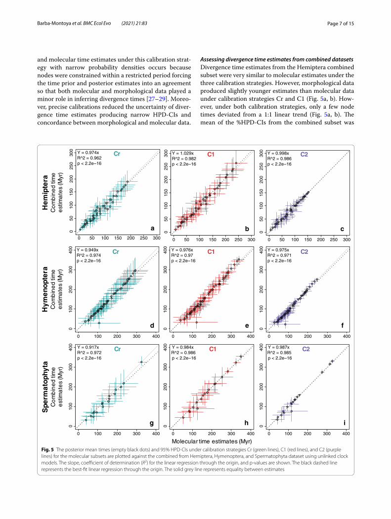
and molecular time estimates under this calibration strat-egy with narrow probability densities occurs because nodes were constrained within a restricted period forcing the time prior and posterior estimates into an agreement so that both molecular and morphological data played a minor role in inferring divergence times [27–29]. Moreo-ver, precise calibrations reduced the uncertainty of diver-gence time estimates producing narrow HPD-CIs and concordance between morphological and molecular data.

Assessing divergence time estimates from combined datasetsDivergence time estimates from the Hemiptera combined subset were very similar to molecular estimates under the three calibration strategies. However, morphological data produced slightly younger estimates than molecular data under calibration strategies Cr and C1 (Fig. 5a, b). How-ever, under both calibration strategies, only a few node times deviated from a 1:1 linear trend (Fig.  5a, b). The mean of the %HPD-CIs from the combined subset was

0 50 100 150 200 250 300

050

100

150

200

250

300

Y = 1.029x R^2 = 0.982 p < 2.2e 16

Molecular time estimates (Myr)

Hem

iptera

Co

mb

ine

dtim

ee

stim

ate

s(M

yr)

Hym

enop

tera

Co

mb

ine

dtim

ee

stim

ate

s(M

yr)

Cr

Cr

C1

C1

C2

C2

Cr C1 C2

Spe

rmatop

hyta

Co

mb

ine

dtim

ee

stim

ate

s(M

yr)

a b c

d e f

g h i

0 50 100 150 200 250 300

050

100

150

200

250

300

Y = 0.974x R^2 = 0.962 p < 2.2e 16

0 50 100 150 200 250 300

050

100

150

200

250

300

Y = 0.998x R^2 = 0.986 p < 2.2e 16

0 100 200 300 400

010

020

030

040

0

Y = 0.976x R^2 = 0.97 p < 2.2e 16

0 100 200 300 400

010

020

030

040

0

Y = 0.949x R^2 = 0.974 p < 2.2e 16

0 100 200 300 400

010

020

030

040

0

Y = 0.975x R^2 = 0.971 p < 2.2e 16

0 100 200 300 400

010

020

030

040

0

Y = 0.984x R^2 = 0.986 p < 2.2e 16

0 100 200 300 400

010

020

030

040

0

Y = 0.917x R^2 = 0.972 p < 2.2e 16

0 100 200 300 400

010

020

030

040

0

Y = 0.987x R^2 = 0.985 p < 2.2e 16

Fig. 5 The posterior mean times (empty black dots) and 95% HPD‑CIs under calibration strategies Cr (green lines), C1 (red lines), and C2 (purple lines) for the molecular subsets are plotted against the combined from Hemiptera, Hymenoptera, and Spermatophyta dataset using unlinked clock models. The slope, coefficient of determination (R2) for the linear regression through the origin, and p‑values are shown. The black dashed line represents the best‑fit linear regression through the origin. The solid grey line represents equality between estimates

Page 8 of 15Barba‑Montoya et al. BMC Ecol Evo (2021) 21:83

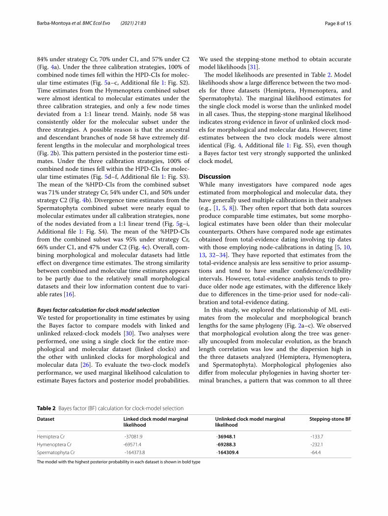
84% under strategy Cr, 70% under C1, and 57% under C2 (Fig. 4a). Under the three calibration strategies, 100% of combined node times fell within the HPD-CIs for molec-ular time estimates (Fig. 5a–c, Additional file 1: Fig. S2). Time estimates from the Hymenoptera combined subset were almost identical to molecular estimates under the three calibration strategies, and only a few node times deviated from a 1:1 linear trend. Mainly, node 58 was consistently older for the molecular subset under the three strategies. A possible reason is that the ancestral and descendant branches of node 58 have extremely dif-ferent lengths in the molecular and morphological trees (Fig. 2b). This pattern persisted in the posterior time esti-mates. Under the three calibration strategies, 100% of combined node times fell within the HPD-CIs for molec-ular time estimates (Fig. 5d–f, Additional file 1: Fig. S3). The mean of the %HPD-CIs from the combined subset was 71% under strategy Cr, 54% under C1, and 50% under strategy C2 (Fig. 4b). Divergence time estimates from the Spermatophyta combined subset were nearly equal to molecular estimates under all calibration strategies, none of the nodes deviated from a 1:1 linear trend (Fig. 5g–i, Additional file  1: Fig. S4). The mean of the %HPD-CIs from the combined subset was 95% under strategy Cr, 66% under C1, and 47% under C2 (Fig. 4c). Overall, com-bining morphological and molecular datasets had little effect on divergence time estimates. The strong similarity between combined and molecular time estimates appears to be partly due to the relatively small morphological datasets and their low information content due to vari-able rates [16].

Bayes factor calculation for clock model selectionWe tested for proportionality in time estimates by using the Bayes factor to compare models with linked and unlinked relaxed-clock models [30]. Two analyses were performed, one using a single clock for the entire mor-phological and molecular dataset (linked clocks) and the other with unlinked clocks for morphological and molecular data [26]. To evaluate the two-clock model’s performance, we used marginal likelihood calculation to estimate Bayes factors and posterior model probabilities.

We used the stepping-stone method to obtain accurate model likelihoods [31].

The model likelihoods are presented in Table 2. Model likelihoods show a large difference between the two mod-els for three datasets (Hemiptera, Hymenoptera, and Spermatophyta). The marginal likelihood estimates for the single clock model is worse than the unlinked model in all cases. Thus, the stepping-stone marginal likelihood indicates strong evidence in favor of unlinked clock mod-els for morphological and molecular data. However, time estimates between the two clock models were almost identical (Fig.  4, Additional file  1: Fig. S5), even though a Bayes factor test very strongly supported the unlinked clock model,

DiscussionWhile many investigators have compared node ages estimated from morphological and molecular data, they have generally used multiple calibrations in their analyses (e.g., [1, 5, 8]). They often report that both data sources produce comparable time estimates, but some morpho-logical estimates have been older than their molecular counterparts. Others have compared node age estimates obtained from total-evidence dating involving tip dates with those employing node-calibrations in dating [5, 10, 13, 32–34]. They have reported that estimates from the total-evidence analysis are less sensitive to prior assump-tions and tend to have smaller confidence/credibility intervals. However, total-evidence analysis tends to pro-duce older node age estimates, with the difference likely due to differences in the time-prior used for node-cali-bration and total-evidence dating.

In this study, we explored the relationship of ML esti-mates from the  molecular and morphological  branch lengths for the same phylogeny (Fig. 2a–c). We observed that morphological evolution along the tree was gener-ally uncoupled from molecular evolution, as the branch length correlation was low and the dispersion high in the three datasets analyzed (Hemiptera, Hymenoptera, and Spermatophyta). Morphological phylogenies also differ from molecular phylogenies in having shorter ter-minal branches, a pattern that was common to all three

Table 2 Bayes factor (BF) calculation for clock‑model selection

The model with the highest posterior probability in each dataset is shown in bold type

Dataset Linked clock model marginal likelihood

Unlinked clock model marginal likelihood

Stepping-stone BF

Hemiptera Cr ‑37081.9 ‑36948.1 ‑133.7

Hymenoptera Cr ‑69571.4 ‑69288.3 ‑232.1

Spermatophyta Cr ‑164373.8 ‑164309.4 ‑64.4

Page 9 of 15Barba‑Montoya et al. BMC Ecol Evo (2021) 21:83

datasets. The low correlation suggests that morphologi-cal characters evolve at much more variable rates than molecules, and the shorter terminal branches are likely to be due to ascertainment bias. We expected these disa-greements between molecular and morphological branch lengths to have a significant detrimental impact on the efficacy of dating analysis.

However, the observed concordance between diver-gence times produced by these two types of data seems to be much more than that anticipated based on comparing individual branch lengths. One fundamental reason for this observation is that relative node-to-tip distances in morphological and molecular phylogenies have a much better correlation than the branch lengths (Fig.  6). The node-to-tip distance estimate for a node is the sum of branch lengths of all paths from this node to all descend-ent tips divided by the total number of descendant tips. In the Hemiptera dataset, the correlation between node-to-tip distances (r = 0.708) was much higher than that for the branch lengths (r = 0.409), although the relation-ship was still noisy (Fig.  6a). In the Hymenoptera and the Spermatophyta datasets, the correlation between node-to-tip distances was also high (r = 0.755 and 0.735 respectively) compared to the branch lengths (r = 0.131, and 0.363, respectively). The dispersion was lower for each dataset than that for branch lengths (Fig. 6b, c).

Therefore, a better relationship between node-to-tip distances from morphological and molecular data is a primary reason for the concordance between divergence times produced by these two types of data. The averag-ing of path lengths to multiple descendants in calculating node-to-tip distances is likely creating the time structure

in both molecular and morphological phylogenies, as they have the same branching pattern. If so, we would expect this benefit to be weaker for nodes with fewer descendants because there are fewer evolutionary paths to average over. This effect was observed in the Hemip-tera and Hymenoptera datasets; terminal nodes showed weaker node-to-tip distance relationships reflected in their significant deviation from the linear trend (Fig. 7). The terminal nodes represent the split of one lineage to form two living taxa, for which the r was similar  in the node-to-tip comparison  to that for the branch lengths.

0.0 0.5 1.0 1.5

0.0

0.5

1.0

1.5

Y = 1.905xr = 0.735p = 7e−04

0.0 0.2 0.4 0.6 0.8

0.0

0.2

0.4

0.6

0.8

Y = 1.536xr = 0.755p = 2.7e−11

0.0 0.1 0.2 0.3 0.4 0.5 0.6 0.7

0.0

0.1

0.2

0.3

0.4

0.5

0.6

0.7

Y = 1.02xr = 0.708p = 1.1e−07

Mor

phol

ogic

al

node

-to-

tip d

ista

nces

Molecular node-to-tip distances

Hemiptera Hymenoptera Spermatophyta

a b c

Fig. 6 The linear relationship between node‑to‑tip distances from molecules alone versus morphology for a Hemiptera, b Hymenoptera, and c Spermatophyta. The black dashed line represents the best‑fit linear regression through the origin. The slope, correlation coefficient (r) and p‑values are shown. The black dashed line represents the best‑fit linear regression through the origin. The solid grey line represents equality between estimates

Hemiptera

Hymenoptera

Spermatophyta

r of node-to-tip distances

Terminal nodes Intermediate nodes Deep nodes

0 0.2 0.6 10.80.4

p = 0.655

p = 0.127

p = 0.091

p = 0.001

p = 2.7e 04

p = 2.7e 06

p = 0.034

p = 1.7e 03

p = 0.443

Fig. 7 Linear relationships of molecular and morphological estimates of node‑to‑tip distances for nodes that locate at the terminal (solid), intermediate (open), and deep (hatch) divergence regions for Hemiptera, Hymenoptera, and Spermatophyta. An r of one indicates a perfect linear relationship between molecular and morphological estimates, marked as the gray dashed line. P‑values are shown next to the bars

Page 10 of 15Barba‑Montoya et al. BMC Ecol Evo (2021) 21:83

The linear relationships of molecular and morphologi-cal node-to-tip distance estimates were higher for inter-mediate divergence nodes (Fig.  7). These nodes had at least three descendants, excluding the root and nodes representing the set of deep divergence nodes. Then, the linear relationships of molecular and morphological node-to-tip distance estimates of the deepest nodes were also higher than  for terminal nodes. This suggests that for the Hemiptera  and Hymenoptera datasets, tip-cal-ibration methods might be better suited for nodes with many taxa. However, the linear relationships of molecu-lar and morphological node-to-tip distance estimates of the intermediate nodes were the lowest in the Spermato-phyta dataset, indicating discordance of estimated dates for intermediate  nodes. Therefore, tip-calibration meth-ods might be better suited for deep  and shallow nodes for  this dataset (Fig.  7). Based on our results, it seems possible that the duration of the branches connecting fossils to the extant tree, which are determined based on morphological evidence, may not be wrongly inferred for deepest and intermediate nodes in tip-calibration and FBD dating approaches (see also, Püschel et al. [20]). The discordance observed is because the Bayesian dat-ing analysis tends to be too sensitive to BD (birth–death) process used to specify the time prior without constraints on interior nodes [24].

Moreover, the high concordance of relative time esti-mates between morphological and molecular data when multiple internal calibrations are applied, and the

extreme similarity of time estimates between combined and molecular data, justify the use of morphological data in node-, tip-calibration and FBD dating approach. This kind of analysis is especially useful for total-evidence approaches because they are likely impacted by the rela-tionship between morphological and molecular esti-mates, in contrast to node-dating approaches that do not use morphological data. Nevertheless, the concordance of time estimates between datasets needs to be carefully examined. As we showed, discordance on time structure can only be corrected by calibrations, but some nodes remain different (e.g., Hemiptera nodes 58 and 59; Hyme-noptera nodes 58 73, 74, 75, and 85; Spermatophyta node 28. Additional file 1: Figs. S2, S3, S4; nodes are numbered as in Fig. 8a–c).

We examined if the high correlation between morpho-logical and molecular time estimates could arise due to using the same topology and speciation tree prior in the Bayesian analysis (suggested by S. Guindon). We gen-erated time estimates using a uniform BD branching process in MCMCTree [35], conditioning on the topol-ogy and root node calibration. Neither molecular nor morphological data were used. The correlation between the resulting times was determined to evaluate the time structure imposed by the tree prior when the tree topol-ogy is fixed. The correlation between node times gen-erated using a uniform BD branching process and time estimates obtained from molecular and morphologi-cal data was high for the three datasets (R2 = 0.733, 0.5

111

Taxonus

Gilpinia

Paremphytus

Cephus

Urocerus

Ichneumonidae

Megalodontes_C

Acordulecera

Evanioidea

Diprion

Macroxyela

Metallus

PamphiliusCephalcia

Xiphydria

LophyrotomaPhylacteophaga

Aglaostigma

Selandria

Neurotoma

Xeris

Vespidae

Syntexis

Perga

Onycholyda

Runaria

Dolerus

Apoidea_A

ArgeSterictiphora

Decameria

Megalodontes_SK

Monophadnoides

Blasticotoma

Tenthredo

Cladius

Corynis

Trigonalidae

Abia

Sirex

Hoplocampa

Calameuta

Tremex

Stephanidae_sp_A

Acantholyda

Cynipoidea

Xyela

Nematus

Megalyra

Nematinus

Strongylogaster

Cimbicinae

Orussus

AthaliaMonoctenus

Hartigia

110

109

107

106

105

104

103

102

101100

99

98

97

9695

94

9392

9190

89

8887

86

85

84

8382

81

80

77

76

7574

7372

71

70

6867

66

6564

6261

60

59

58

63

57

7978

69

108

Juniperus

SarcandraSaruma

Nuphar

PinusCedrus

Cunninghamia

Cycas

Amborella

Taxus

Ephedra

Houttuynia

Prumnopitys

Zamia

Kadsura

WelwitschiaGnetum

Ginkgo

3334

32

28

2625

24

2322

21

36

35

30

27

20

29

31

c

Eulecanium_tiliae

Eriococcus_coccineus

Conchaspis_lata

Puto_yuccae

Coelostomidia_wairoensis

Crypticerya_genistae

Marchalina_hellenica

Gallacoccus_secundus

Insignorthezia_insignis

Bambusaspis_miliaris

Kuwania_quercus

Chionaspis_salicis

Eumargarodes_laingi

Tanyscelis_verrucula

Aonidiella_aurantii

Newsteadia_floccosa

Dactylopius_confususCeroplastes_japonicus

Ovaticoccus_agavium

Beesonia_dipterocarpi

Stictococcus_vayssievei

Coccus_hesperidum

Pseudococcus_longispinus

Parlatoria_oleae

Icerya_seychellarum

Eriococcus_buxi

Planococcus_citriFerrisia_virgata

Phoenicococcus_martelli

Kermes_quercus

Aclerda_arundinariae

Matsucoccus_matsumurae

Antonina_graminis_crawi

Coelostomidia_pilosa

Neosteingelia_texana

Pseudococcus_maritimus

Puto_superbus

Drosicha_pinicola

Icerya_purchasi

Lecanodiaspis_baculifera

Gigantococcus_maximus

Dysmicoccus_alazon

Drosicha_corpulenta

Orthezia_urticae90

89

88

87

86

85

8483

82

81

80

70

78

76

75

73

69

71

68

67

66

65

63

6261

60

5958

57

5352

51

5655

54

91

72

74

79

77

64

4950a

b

Fig. 8 Phylogenies for a 44 Hemiptera species, b 56 Hymenoptera species, and c 18 Spermatophyta species. Closed red dots indicate calibration nodes

Page 11 of 15Barba‑Montoya et al. BMC Ecol Evo (2021) 21:83

and 0.84 for molecular subsets and R2 = 0.841, 0.726 and 0.722 for morphological subsets), rivaling the correlation between molecular and morphological time estimates (R2 = 0.677, 0.801, 0.844 for Hemiptera, Hymenoptera and Spermatophyta, respectively). While we expected some correlation because of the same time prior and branching process, which results in drawing times from the same probability distribution of times for each node in the phylogeny [24], the magnitude of correlation observed was surprising. Therefore, the species phylog-eny and the use of the same tree-prior would introduce similar time structures for different data types in their joint Bayesian analysis. In the future, we plan to examine how this correlation of time structure affects the accu-racy of Bayesian node age estimates, as compared to the performance non-Bayesian methods that estimate times based primarily on branch lengths without using any spe-ciation tree-priors (Tao et al. 2020).

ConclusionsOverall, our study allows us to conclude that (1) relative ML branch lengths between morphological and molecu-lar characters were very different, but relative node-to-tip distances were considerably more concordant, suggest-ing a much more concordant time structure in the mor-phological and molecular dataset than that captured in the comparison of branch lengths. (2) When no internal calibrations were applied, morphological and molecular clock produced time estimates with a high correlation, which may be caused by the same speciation tree prior applied in the joint consideration of molecular and mor-phological data in the Bayesian analyses. The concord-ance between time estimates was improved by applying multiple and/or narrow internal calibrations. (3) The combination of molecular and morphological data gen-erally resulted in time estimates nearly identical to the ones from molecular data alone. Our study allows us to conclude that although there is a concordant time struc-ture in morphological and molecular data, the interpre-tation of fossil ages is determinant for the agreement of time estimates from morphological and molecular clock analyses. We emphasize the importance of evaluating the concordance of time structure in morphological and molecular data before any dating analysis using com-bined datasets.

MethodsTaxon sampling, molecular and morphological data, and tree topologiesFor comparison between results from molecules and morphology, we composed three datasets consisting of extant species, for which both molecular and morpho-logical data were available. Thus, extinct taxa were not

included in our matrices. First, a dataset of 174 discrete morphological characters and 3731 molecular charac-ters (base pairs—bp) from 44 Hemiptera species was obtained from Vea and Grimaldi (2016) [32]. Second, a dataset of 353 discrete morphological characters and 5096 molecular characters (bp) from 55 Hymenoptera species was taken from Ronquist et al. (2012) [10]. Third, a dataset of 121 discrete morphological characters and 19,870 molecular characters (bp) from 18 Spermatophyta species was obtained from Doyle (2006) [36] and Morris et al. (2018) [37], respectively. Three rooted trees (Fig. 8) were constructed based on the literature: one for Hemip-tera species [32], one for Hymenoptera species [10], and one for Spermatophyta species [37]. The three topologies from Fig. 8 were fixed in all analyses to ensure consistent calibrations and avoid the confounding effects of alterna-tive phylogenies and calibrations. Moreover, the use of a phylogeny reliably inferred as a fixed topology for dating is a common practice (e.g., [7, 37–40]).

Fossil calibrations and calibration strategiesFossil calibrations are the foremost source of information for translating the distances between molecular/morpho-logical sequences into estimates of absolute times and absolute rates in clock dating analysis. Thus, the calibra-tions’ quality is expected to impact divergence time esti-mates significantly, even if a large amount of sequence data is available. Therefore, we employed three fossil cali-bration strategies simulating different quality of calibra-tions based on fossil evidence. Fossil calibrations were employed following justifications from the original stud-ies (Hemiptera [32], Hymenoptera [10], Spermatophyta [27]; Fig.  8 and Table  3). For the three strategies, node calibrations were specified using a uniform distribution from fossil minimum-ages (Table 3).

Calibration strategy CrOnly one calibration on the root was specified (no inter-nal calibrations), assigning a uniform distribution bor-rowed from calibration strategy C1 as described below (Table  3). This strategy reflects a poor fossil record and the lack of fossil evidence for the internal nodes. How-ever, it has the advantage of being the baseline for exam-ining the impact of using calibration constraints on divergence time estimates.

Calibration strategy C1Calibrations were specified using a uniform distribu-tion U(tL, tU), where tL is the minimum age bound and tU the maximum age bound, with mean tM =

1

2(tL + tU) .

The offset and mean values from the original calibration were used respectively as the minimum bound (tL) and

Page 12 of 15Barba‑Montoya et al. BMC Ecol Evo (2021) 21:83

mean (tM) for the uniform distribution so that the maxi-mum bound was tU =

tM0.5

− tL (Table  3). This strategy reflects agnosticism about the true time of divergence between these bounds, which is considered a more real-istic scenario.

Calibration strategy C2Calibrations were also specified using a uniform distri-bution U(tL, tU). The offset value from the original expo-nential distribution was used as the minimum bound (tL), and the maximum bound was specified at tU = tL +

tL10

, which assigns a probability of 10% for the minimum bound (tL) to be older (Table  3). This strategy reflects a prior belief that the fossil minima are a close approxima-tion of clade age. Such a strategy is only appropriate for calibration nodes within a restricted time, assuming that fossil ages represent the "true" age of the corresponding lineage.

Modeling morphological and molecular evolutionTo model morphological evolution, we used the Mk model [15], with the ascertainment bias set to variable (only variable characters scored), equal state frequencies, and assuming discrete gamma-distributed heterogeneity among sites (Mk + Γ5). To model molecular evolution, we

used the GTR general time-reversible (GTR) model [41], with discrete gamma-distributed heterogeneity among sites (GTR + Γ5). Unlike the model applied for morpho-logical data (Mk + Γ5), the GTR + Γ5 model relaxes the assumption of equal character frequencies in molecular substitutions. A ML optimization of model parameters and branch lengths for the given topology was performed for both molecular and morphological data separately in MEGAX [42] and RAxML [43], respectively, for the Hemiptera, Hymenoptera, and Spermatophyta datasets to assess the pattern of branches lengths from the mor-phological and molecular subsets. Tests of proportional-ity of branch lengths were performed using a likelihood ratio test to compare nested models with either linked or unlinked branch lengths in RAxML-ng [44]. We also cal-culated the node-to-tip distances using the ML trees. For each node, the node-to-tip distance is the sum of branch lengths of all paths from this node to all descendent tips divided by the total number of descendant tips.

Bayesian divergence time estimationIn each data analysis (Hemiptera, Hymenoptera, and Spermatophyta), we used one molecular subset, one morphological subset, and one combined (morphologi-cal + molecular) subset, and applied three calibration

Table 3 Summary of fossil calibrations and calibration strategies used in this study in million years before the present

Nodes are numbered as in Fig. 8. Fossil taxa are indicated by a dagger (†) before their names. N/A, not applicable

Dataset Node Clade Minimum divergence time (Ma) Calibration strategy Cr

Calibration strategy C1

Calibration strategy C2

Hemiptera 91 (root) Coccomorpha 140 (†Eomatsucoccus casei) U(140,340) U(140,340) U(140,354)

Hemiptera 79 Kuwaniidae 45 (†Hoffeinsia foldi) N/A U(45,155) U(45,50)

Hemiptera 77 Ortheziidae 135 (†Cretorhezia hammanaica) N/A U(135,145) U(135,149)

Hemiptera 74 Putoidae 45 (†Puto sp.) N/A U(45,155) U(45,50)

Hemiptera 72 Pseudococcidae 135 (†Williamsicoccus megalops) N/A U(135,145) U(135,149)

Hemiptera 64 Coccidae 98 (†Rosahendersonia prisca) N/A U(98,122) U(98,108)

Hemiptera 50 Diaspididae 50 (†Normarkicoccus cambayae) N/A U(50,150) U(50,55)

Hymenoptera 111 (root) Hymenoptera 235 (†Triassoxyela, Asioxyela) U(235,369) U(235,369) U(235,259)

Hymenoptera 108 Tenthredinoidea 140 (†Palaeathalia) N/A U(140,328) U(140,154)

Hymenoptera 79 Vespina 180 (†Brigittepteris) N/A U(180,290) U(180,198)

Hymenoptera 78 Apocrita 176 (†Cleistogaster) N/A U(176,294) U(176,194)

Hymenoptera 69 Siricoidea 161 (†Aulisca) N/A U(161,309) U(161,177

Hymenoptera 63 Pamphiloidea 161 (†Aulidontes, Pamphilidae sp.) N/A U(161,309) U(161,177)

Hymenoptera 57 Xylidae 180 (†Eoxyela) N/A U(180,298) U(180,198)

Spermatophyta 36 (root) Spermatophytes 308.14 (†Cordaites iowensis) U(308,366) U(308,366) U(308,339)

Spermatophyta 35 Angiosperms 125.9 (tricolpate pollen) N/A U(126,247) U(126,139)

Spermatophyta 31 Stem‑Saururus 44.3 (†Saururus tuckerae) N/A U(44,247) U(44,48)

Spermatophyta 30 Acrogymnosperms 308.14 (†Cordaties iowensis) N/A U(308,366) U(308,339)

Spermatophyta 29 Gingko‑Cycas 264.7 (†Crossozamia) N/A U(265,366) U(265,282)

Spermatophyta 27 Conifers 147 (†Rissikia media) N/A U(147,312) U(147,162)

Spermatophyta 20 Gnetales 119.6 (†Eoantha zherkihinii) N/A U(120,312) U(120,132)

Page 13 of 15Barba‑Montoya et al. BMC Ecol Evo (2021) 21:83

strategies, Cr, C1, and C2. All Bayesian analyses (27 in total) were carried out with the program MrBayes [31]. The sequence likelihood of the morphological and molecular subsets was calculated under the Mk + Γ5 and the GTR + Γ5 substitution models, respectively. The com-bined subset was treated as two partitions under sepa-rate substitution models (Mk + Γ5, and GTR + Γ5), with separate substitution-rate parameters assigned and esti-mated for each partition. Two sets of analyses were per-formed, using: a single clock for the entire morphological and molecular dataset (linked clocks) or unlinked clocks for morphological and molecular data [26]. The MCMC sampling settings were determined through pilot runs and differed among the datasets. We ran each analysis at least twice and checked for convergence by compar-ing the posterior mean estimates between runs and plot-ting the samples’ time series traces. We then merged the samples from the runs before summarizing the posterior. Moreover, we ran analyses without sequence data to esti-mate the effective time prior that informed the result-ing marginal priors for the node ages after truncation. We plotted these alongside node age estimates from the posteriors to assess how much the data influences age estimates (Additional file  1: Figs. S2, S3, S4). The prior settings and the MCMC run parameters of each data-set analysis are detailed below. For the Bayes factor test, marginal likelihoods were estimated using stepping-stone sampling based on 50 steps with 490,000 generations (490 samples) within each step.

Analysis of Hemiptera datasetAnalyses were performed on three subsets from 44 Hemiptera species, one of 174 morphological charac-ters with 12.15% of missing data; one of 3731 molecular characters (bp) with 47.96% of missing data; and one combined subset (morphological + molecular) of 3905 characters with 46.36% of missing data. The rooted tree topology with seven calibration nodes (Fig. 8a) was fixed in all analyses. Detailed information on the calibrations is given in Table 3. Models of evolution for each subset were implemented, as described earlier. Priors for rates were set as in Vea and Grimaldi (2016) [32]. The Independent Gamma Rate (IGR) model, in which the rates of evolu-tion on branches varied independently from a gamma distribution [45], was used as a rate prior. The gamma model is parametrized using two parameters: the mean and variance. The time unit was 100 Myr. The mean was assigned a lognormal hyperprior L.N. (− 6.0605,0.0519), with the mean of exp{− 6.0605 + 0.05192/2} = 0.0023. The variance (Igrvarpr) was assigned an exponential hyperp-rior with a mean of 0.039. Analyses were performed with either linked or unlinked relaxed clock models (i.e., link Igrvar = (all)) or unlink Igrvar = (all)). For each analysis,

four MCMC runs were performed, each consisting of 5 × 106 iterations, sampling every 200, with the burn-in set to 10%, resulting in a total of 9 × 104 samples from the four runs, which were used to obtain posterior time estimates.

Analysis of Hymenoptera datasetAnalyses were performed on three subsets from 56 Hymenoptera species; one of 353 morphological char-acters with 19.97% of missing data; one of 5096 molecu-lar characters (bp) with 25.65% of missing data; and one combined subset (morphological + molecular) of 5449 characters with 25.28% of missing data. The rooted tree topology with seven calibration nodes (Fig. 8b) was fixed in all analyses. Detailed information on the calibrations is given in Table  3. Models of evolution for each sub-set were implemented, as described earlier. Priors for rates were set as in Ronquist et  al. (2012) [10] for the three subsets. The IGR model was used to specify prior for rates. The time unit was 100 Myr. The mean of the gamma was assigned a lognormal hyperprior LN(− 7.1, 0.5), with the mean exp{− 7.1 + 0.52/2} = 0.001. The vari-ance of the gamma was assigned an exponential hyperp-rior with a mean of 0.027. Analyses were performed with either linked or unlinked relaxed clock models (i.e., link Igrvar = (all)) or unlink Igrvar = (all)). Four MCMC runs were performed, each consisting of 5 × 106 iterations, sampling every 200, with the burn-in set to 10%, resulting in a total of 9 × 104 samples from the four runs.

Analysis of Spermatophyta datasetAnalyses were performed on three subsets from 18 Sper-matophyta species; one of 121 morphological charac-ters with 27.5% of missing data; one of 19,870 molecular characters (bp) with 14.11% of missing data; and one combined subset (morphological + molecular) of 5449 characters with 14.18% of missing data. The rooted tree topology with seven calibration nodes (Fig. 8c) was fixed in all analyses. Detailed information on the calibrations is given in Table 3. Models of evolution for each subset were implemented, as described earlier. Priors for rates were set as in Barba-Montoya et  al. (2018) [27] for the three subsets. The IGR model was used to specify prior for rates. The time unit was 100 Myr. The mean of the gamma was assigned a lognormal hyperprior LN (− 2.79, 0.5), with the mean exp{− 2.79 + 0.52/2} = 0.07, and the variance of the gamma is assigned an exponential hyper-prior with a mean of 0.1. Analyses were performed with either linked or unlinked relaxed clock models (i.e., link Igrvar = (all)) or unlink Igrvar = (all)). Six MCMC runs were performed, each consisting of 1 × 107 iterations,

Page 14 of 15Barba‑Montoya et al. BMC Ecol Evo (2021) 21:83

sampling every 200, with the burn-in set to 10%, resulting in a total of 2.7 × 105 samples from all six runs.

AbbreviationsFBD: Fossilized birth–death; ML: Maximum likelihood; CIs: Credibility intervals; BF: Bayes factor; BD: Birth–death; bp: Base pairs; GTR : General time‑reversible.

Supplementary InformationThe online version contains supplementary material available at https:// doi. org/ 10. 1186/ s12862‑ 021‑ 01798‑6.

Additional file 1: Figure S1. The linear relationship between internal branch lengths obtained from molecules versus morphology (excluding terminal branches) for (A) Hemiptera, (B) Hymenoptera, and (C) Sperma‑tophyta. The slope, correlation coefficient (r) and p‑values are shown. The black dashed line represents the best‑fit linear regression through the origin. The solid grey line represents equality between estimates. Figure S2. Calibration densities (dark grey bands), 95% HPD‑CIs in the time prior (light grey bands), and posterior (colored lines) for 47 nodes in the Hemiptera timetrees under calibration strategies (A) Cr‑green, (B) C1‑red, and (C) C2‑purple. Figure S3. Calibration densities (dark grey bands), 95% HPD‑CIs in the time prior (light grey bands), and posterior (colored lines) for 55 nodes in the Hymenoptera timetrees under calibration strategies (A) Cr‑green, (B) C1‑red, and (C) C2‑purple. Figure S4. Calibration densities (dark grey bands), 95% HPD‑CIs in the time prior (light grey bands), and posterior (colored lines) for 17 nodes in the Spermatophyta timetrees under calibration strategies (A) Cr‑green, (B) C1‑red, and (C) C2‑purple. Figure S5. The posterior mean times (empty black dots) and 95% HPD‑CIs under calibration strategies Cr (green lines), C1 (red lines), and C2 (purple lines) for the molecular subsets are plotted against the combined from Hemiptera, Hymenoptera, and Spermatophyta datasets using linked clock models.

AcknowledgementsWe thank Aishwarya Durgam for technical support and Dr. Beatriz Mello for comments and editorial suggestions.

Authors’ contributionsSK and JBM designed the study. JBM and QT assembled the datasets. JBM performed the analyses. JBM and SK wrote the manuscript. All authors read and approved the final manuscript.

FundingThis research was supported in part by grants from the National Institutes of Health (NIH GM0126567‑03) and National Science Foundation (NSF 1661218 and 1932765) to S.K.

Availability of data and materialsThe datasets generated and/or analyzed during the current study are available in the figshare repository: https:// doi. org/ 10. 6084/ m9. figsh are. 97757 30. [46].

Declarations

Ethics approval and consent to participateNot applicable.

Consent for publicationNot applicable.

Competing interestsThe authors declare that they have no competing interests.

Author details1 Institute for Genomics and Evolutionary Medicine, Temple University, Philadelphia, PA 19122, USA. 2 Department of Biology, Temple University,

Philadelphia, PA 19122, USA. 3 Center for Excellence in Genome Medicine and Research, King Abdulaziz University, Jeddah, Saudi Arabia.

Received: 12 May 2020 Accepted: 20 April 2021

References 1. Schrago CG, Mello B, Soares AER. Combining fossil and molecular

data to date the diversification of New World Primates. J Evol Biol. 2013;26:2438–46.

2. Beck RMD, Lee MSY. Ancient dates or accelerated rates? Morpho‑logical clocks and the antiquity of placental mammals. Proc R Soc B. 2014;281:20141278.

3. Lee MSY, Cau A, Naish D, Dyke GJ. Morphological clocks in paleontology, and a mid‑cretaceous origin of crown aves. Syst Biol. 2014;63:442–9.

4. Matzke NJ, Wright A. Inferring node dates from tip dates in fossil Canidae: the importance of tree priors. Biol Lett. 2016;12:20160328.

5. Puttick MN, Thomas GH, Benton MJ. Dating placentalia: morphological clocks fail to close the molecular fossil gap. Evolution. 2016;70:873–86.

6. King B, Qiao T, Lee MSY, Zhu M, Long JA. Bayesian morphological clock methods resurrect placoderm monophyly and reveal rapid early evolu‑tion in jawed vertebrates. Syst Biol. 2017;66:499–516.

7. Álvarez‑Carretero S, Goswami A, Yang Z, Dos Reis M. Bayesian estimation of species divergence times using correlated quantitative characters. Syst Biol. 2019;68:967–86.

8. Caldas IV, Schrago CG. Data partitioning and correction for ascertain‑ment bias reduce the uncertainty of placental mammal divergence times inferred from the morphological clock. Ecol Evol. 2019;9:2255–62.

9. Pyron RA. Divergence time estimation using fossils as terminal taxa and the origins of lissamphibia. Syst Biol. 2011;60:466–81.

10. Ronquist F, Klopfstein S, Vilhelmsen L, Schulmeister S, Murray DL, Rasnit‑syn AP. A total‑evidence approach to dating with fossils, applied to the early radiation of the hymenoptera. Syst Biol. 2012;61:973–99.

11. Ronquist F, Lartillot N, Phillips MJ, Lyon CB. Closing the gap between rocks and clocks using total‑evidence dating. Philos Trans R Soc Lond B. 2016;371:20150136.

12. Wood HM, Matzke NJ, Gillespie RG, Griswold CE. Treating fossils as termi‑nal taxa in divergence time estimation reveals ancient vicariance patterns in the palpimanoid spiders. Syst Biol. 2013;62:264–84.

13. O’Reilly JE, dos Reis M, Donoghue PCJ. Dating tips for divergence‑time estimation. Trends Genet. 2015;31:637–50.

14. Gavryushkina A, Heath TA, Ksepka DT, Stadler T, Welch D, Drummond AJ. Bayesian total‑evidence dating reveals the recent crown radiation of penguins. Syst Biol. 2017;66:57–73.

15. Lewis PO. A likelihood approach to estimating phylogeny from discrete morphological character data. Syst Biol. 2001;50:913–25.

16. dos Reis M, Donoghue PCJ, Yang Z. Bayesian molecular clock dating of species divergences in the genomics era. Nat Rev Genet. 2016;17:71–80.

17. Heath TA, Huelsenbeck JP, Stadler T. The fossilized birth–death process for coherent calibration of divergence‑time estimates. Proc Natl Acad Sci USA. 2014;111:E2957–66.

18. Zhang C, Stadler T, Klopfstein S, Heath TA, Ronquist F. Total‑evidence dat‑ing under the fossilized birth‑death process. Syst Biol. 2016;65:228–49.

19. Luo A, Duchene D, Zhang C, Zhu C‑D, Ho SYW. A simulation‑based evalu‑ation of total‑evidence dating under the fossilized birth‑death process. bioRxiv. 2018. https:// doi. org/ 10. 1101/ 436303.

20. Püschel HP, O’Reilly JE, Pisani D, Donoghue PCJ. The impact of fossil stratigraphic ranges on tip‑calibration, and the accuracy and precision of divergence time estimates. Palaeontology. 2019. https:// doi. org/ 10. 1111/ pala. 12443.

21. Klopfstein S, Ryer R, Coiro M, Spasojevic T. Mismatch of the morphology model is mostly unproblematic in total‑evidence dating: insights from an extensive simulation study. bioRxiv. 2019. https:// doi. org/ 10. 1101/ 679084.

22. Bromham L, Duchêne S, Hua X, Ritchie AM, Duchêne DA, Ho SYW. Bayesian molecular dating: opening up the black box. Biol Rev. 2018;93:1165–91.

Page 15 of 15Barba‑Montoya et al. BMC Ecol Evo (2021) 21:83

• fast, convenient online submission

•

thorough peer review by experienced researchers in your field

• rapid publication on acceptance

• support for research data, including large and complex data types

•

gold Open Access which fosters wider collaboration and increased citations

maximum visibility for your research: over 100M website views per year •

At BMC, research is always in progress.

Learn more biomedcentral.com/submissions

Ready to submit your researchReady to submit your research ? Choose BMC and benefit from: ? Choose BMC and benefit from:

23. Goloboff PA, Pittman M, Pol D, Xu X. Morphological data sets fit a com‑mon mechanism much more poorly than DNA sequences and call into question the Mkv model. Syst Biol. 2019;68:494–504.

24. Barba‑Montoya J, dos Reis M, Yang Z. Comparison of different strategies for using fossil calibrations to generate the time prior in Bayesian molecu‑lar clock dating. Mol Phylogenet Evol. 2017;114:386–400.

25. Kimura M. The neutral theory of molecular evolution. In: Molecular evolu‑tionary rates contrasted with phenotypic evolutionary rates. Cambridge: Cambridge University Press; 1983. p. 55–97.

26. Lee MSY. Multiple morphological clocks and total‑evidence tip‑dating in mammals. Biol Lett. 2016;12:20160033.

27. Barba‑Montoya J, dos Reis M, Schneider H, Donoghue PCJ, Yang Z. Constraining uncertainty in the timescale of angiosperm evolution and the veracity of a Cretaceous Terrestrial Revolution. New Phytol. 2018;218:819–34.

28. Magallón S, Gómez‑Acevedo S, Sánchez‑Reyes LL, Hernández‑Hernández T. A metacalibrated time‑tree documents the early rise of flowering plant phylogenetic diversity. New Phytol. 2015;207:437–53.

29. Magallón S, Hilu KW, Quandt D. Land plant evolutionary timeline: gene effects are secondary to fossil constraints in relaxed clock estimation of age and substitution rates. Am J Bot. 2013;100:556–73.

30. Duchêne S, Foster CSP, Ho SYW. Estimating the number and assign‑ment of clock models in analyses of multigene datasets. Bioinformatics. 2016;32:1281–5.

31. Ronquist F, Teslenko M, Van Der Mark P, Ayres DL, Darling A, Höhna S, et al. Mrbayes 3.2: efficient bayesian phylogenetic inference and model choice across a large model space. Syst Biol. 2012;61:539–42.

32. Vea IM, Grimaldi DA. Putting scales into evolutionary time : the diver‑gence of major scale insect lineages (Hemiptera) predates the radiation of modern angiosperm hosts. Sci Rep. 2016;6:1–11.

33. Cascini M, Mitchell KJ, Cooper A, Phillips MJ. Reconstructing the evolution of giant extinct kangaroos: comparing the utility of DNA, morphology, and total evidence. Syst Biol. 2019;68:520–37.

34. Arcila D, Pyron RA, Tyler JC, Ortí G, Betancur R. An evaluation of fossil tip‑dating versus node‑age calibrations in tetraodontiform fishes (Teleostei: Percomorphaceae). Mol Phylogenet Evol. 2015;82:131–45.

35. Yang Z. PAML 4: phylogenetic analysis by maximum likelihood. Mol Biol Evol. 2007;24:1586–91.

36. Doyle JA. Seed ferns and the origin of angiosperms. J Torrey Bot Soc. 2006;133:169–209.

37. Morris JL, Puttick MN, Clark JW, Edwards D, Kenrick P, Pressel S, et al. The timescale of early land plant evolution. Proc Natl Acad Sci USA. 2018. https:// doi. org/ 10. 1073/ pnas. 17195 88115.

38. Dos RM, Gunnell GF, Barba‑Montoya J, Wilkins A, Yang Z, Yoder AD. Using phylogenomic data to explore the effects of relaxed clocks and calibra‑tion strategies on divergence time estimation: primates as a test case. Syst Biol. 2018. https:// doi. org/ 10. 1093/ sysbio/ syy001.

39. Oliveros CH, Field DJ, Ksepka DT, Keith Barker F, Aleixo A, Andersen MJ, et al. Earth history and the passerine superradiation. Proc Natl Acad Sci USA. 2019;116:7916–25.

40. Li HT, Yi TS, Gao LM, Ma PF, Zhang T, Yang JB, et al. Origin of angiosperms and the puzzle of the Jurassic gap. Nat Plants. 2019;5:461–70.

41. Tavaré S. Some probabilistic and statistical problems on the analysis of DNA sequences. Lect Math life Sci. 1986;17:57–86.

42. Kumar S, Stecher G, Li M, Knyaz C, Tamura K. MEGA X: molecular evo‑lutionary genetics analysis across computing platforms. Mol Biol Evol. 2018;35:1547–9.

43. Stamatakis A. RAxML version 8: a tool for phylogenetic analysis and post‑analysis of large phylogenies. Bioinformatics. 2014;30:1312–3.

44. Kozlov AM, Darriba D, Flouri T, Morel B, Stamatakis A. RAxML‑NG: a fast, scalable and user‑friendly tool for maximum likelihood phylogenetic inference. Bioinformatics. 2019;35:4453–5.

45. Lepage T, Bryant D, Philippe H, Lartillot N. A general comparison of relaxed molecular clock models. Mol Biol Evol. 2007;24:2669–80.

46. Barba‑Montoya J, Tao Q, Kumar S. Data from: molecular and morphologi‑cal clocks for estimating evolutionary divergence times. figshare. 2021. https:// doi. org/ 10. 6084/ m9. figsh are. 97757 30.

Publisher’s NoteSpringer Nature remains neutral with regard to jurisdictional claims in pub‑lished maps and institutional affiliations.