molecular hydrodynamics of the moving contact line in two
TRANSCRIPT
COMMUNICATIONS IN COMPUTATIONAL PHYSICSVol. 1, No. 1, pp. 1-52
Commun. Comput. Phys.February 2006
Molecular Hydrodynamics of the Moving Contact
Line in Two-phase Immiscible Flows
Tiezheng Qian1,∗, Xiao-Ping Wang1 and Ping Sheng2
1 Department of Mathematics, The Hong Kong University of Science and Technology,
Clear Water Bay, Kowloon, Hong Kong, China.2 Department of Physics, The Hong Kong University of Science and Technology, Clear
Water Bay, Kowloon, Hong Kong, China.
Received 1 June 2005; Accepted (in revised version) 17 September 2005
Communicated by Weinan E
Abstract. The no-slip boundary condition, i.e., zero fluid velocity relative to the solid at thefluid-solid interface, has been very successful in describing many macroscopic flows. A problemof principle arises when the no-slip boundary condition is used to model the hydrodynamicsof immiscible-fluid displacement in the vicinity of the moving contact line, where the interfaceseparating two immiscible fluids intersects the solid wall. Decades ago it was already knownthat the moving contact line is incompatible with the no-slip boundary condition, since thelatter would imply infinite dissipation due to a non-integrable singularity in the stress nearthe contact line. In this paper we first present an introductory review of the problem. Wethen present a detailed review of our recent results on the contact-line motion in immiscibletwo-phase flow, from molecular dynamics (MD) simulations to continuum hydrodynamicscalculations. Through extensive MD studies and detailed analysis, we have uncovered theslip boundary condition governing the moving contact line, denoted the generalized Navierboundary condition. We have used this discovery to formulate a continuum hydrodynamicmodel whose predictions are in remarkable quantitative agreement with the MD simulationresults down to the molecular scale. These results serve to affirm the validity of the generalizedNavier boundary condition, as well as to open up the possibility of continuum hydrodynamiccalculations of immiscible flows that are physically meaningful at the molecular level.
Key words: Moving contact line; slip boundary condition; molecular dynamics; continuum hydrody-namics.
∗Correspondence to: Tiezheng Qian, Department of Mathematics, The Hong Kong University of Science andTechnology, Clear Water Bay, Kowloon, Hong Kong, China. Email: [email protected]
http://www.global-sci.com/ 1 c©2005 Global-Science Press
Qian, Wang and Sheng / Commun. Comput. Phys., 1 (2006), pp. 1-52 2
1 Introduction
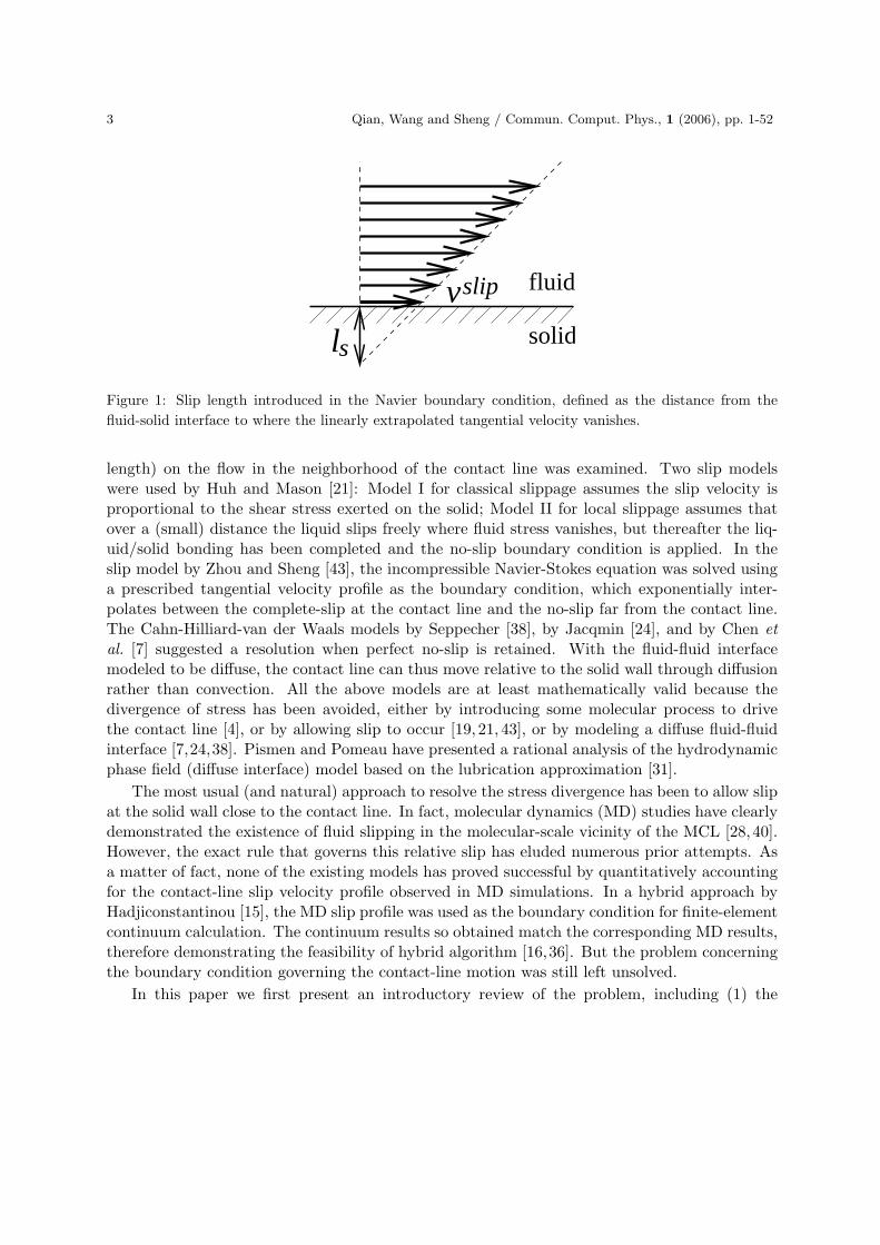
The no-slip boundary condition, i.e., zero relative tangential velocity between the fluid and solidat the interface, serves as a cornerstone in continuum hydrodynamics [3]. Although fluid slippingis generally detected in molecular dynamics (MD) simulations for microscopically small systemsat high flow rate [2, 8, 39, 41], the no-slip boundary condition still works well for macroscopicflows at low flow rate. This is due to the Navier boundary condition which actually accounts forthe slip observed in MD simulations [2, 8, 39,41]. This boundary condition, proposed by Navierin 1823 [30], introduces a slip length ls and assumes that the amount of slip is proportional tothe shear rate in the fluid at the solid surface:
vslip = −lsn ·[
(∇v) + (∇v)T]
,
where vslip is the slip velocity at the surface, measured relative to the (moving) wall, [(∇v)+(∇v)T
]
is the tensor of the rate of strain, and n denotes the outward surface normal (directedout of the fluid). According to the Navier boundary condition, the slip length is defined asthe distance from the fluid-solid interface to where the linearly extrapolated tangential velocityvanishes (see Fig. 1). Typically, ls ranges from a few angstroms to a few nanometers [2,8,39,41].For a flow of characteristic length R and velocity U , the slip velocity is on the order of Uls/R.This explains why the Navier boundary condition is practically indistinguishable from the no-slipboundary condition in macroscopic flows where vslip/U ∼ ls/R → 0.
It has been well known that the no-slip boundary condition is not applicable to the movingcontact line (MCL) where the fluid-fluid interface intersects the solid wall [11,12,20] (see Fig. 2for both the static and moving contact lines). The problem may be simply stated as follows. Inthe two-phase immiscible flow where one fluid displaces another fluid, the contact line appears to“slip” at the solid surface, in direct violation of the no-slip boundary condition. Furthermore, theviscous stress diverges at the contact line if the no-slip boundary condition is applied everywherealong the solid wall. This stress divergence is best illustrated in the reference frame where thefluid-fluid interface is time-independent while the wall moves with velocity U (see Fig. 2b). Asthe fluid velocity has to change from U at the wall (as required by the no-slip boundary condition)to zero at the fluid-fluid interface (which is static), the viscous stress varies as ηU/x, where ηis the viscosity and x is the distance along the wall away from the contact line. Obviously, thisstress diverges as x → 0 because the distance over which the fluid velocity changes from U tozero tends to vanish as the contact line is approached. In particular, this stress divergence isnon-integrable (the integral of 1/x yields lnx), thus implying infinite viscous dissipation.
Over the years there have been numerous models and proposals aiming to resolve the incom-patibility of the no-slip boundary condition with the MCL. For example, there have been thekinetic adsorption/desorption model by Blake [4], the fluid slip models by Hocking [19], by Huhand Mason [21], and by Zhou and Sheng [43], and the Cahn-Hilliard-van der Waals models bySeppecher [38], by Jacqmin [24], and by Chen et al. [7]. In the kinetic adsorption/desorptionmodel by Blake [4], the role of molecular processes was investigated. A deviation of the dynamiccontact angle from the static contact angle was shown to be responsible for the fluid/fluid dis-placement at the MCL. In the slip model by Hocking [19], the effect of a slip coefficient (slip
3 Qian, Wang and Sheng / Commun. Comput. Phys., 1 (2006), pp. 1-52
ls
fluid
solid
vslip
Figure 1: Slip length introduced in the Navier boundary condition, defined as the distance from the
fluid-solid interface to where the linearly extrapolated tangential velocity vanishes.
length) on the flow in the neighborhood of the contact line was examined. Two slip modelswere used by Huh and Mason [21]: Model I for classical slippage assumes the slip velocity isproportional to the shear stress exerted on the solid; Model II for local slippage assumes thatover a (small) distance the liquid slips freely where fluid stress vanishes, but thereafter the liq-uid/solid bonding has been completed and the no-slip boundary condition is applied. In theslip model by Zhou and Sheng [43], the incompressible Navier-Stokes equation was solved usinga prescribed tangential velocity profile as the boundary condition, which exponentially inter-polates between the complete-slip at the contact line and the no-slip far from the contact line.The Cahn-Hilliard-van der Waals models by Seppecher [38], by Jacqmin [24], and by Chen et
al. [7] suggested a resolution when perfect no-slip is retained. With the fluid-fluid interfacemodeled to be diffuse, the contact line can thus move relative to the solid wall through diffusionrather than convection. All the above models are at least mathematically valid because thedivergence of stress has been avoided, either by introducing some molecular process to drivethe contact line [4], or by allowing slip to occur [19, 21, 43], or by modeling a diffuse fluid-fluidinterface [7,24,38]. Pismen and Pomeau have presented a rational analysis of the hydrodynamicphase field (diffuse interface) model based on the lubrication approximation [31].
The most usual (and natural) approach to resolve the stress divergence has been to allow slipat the solid wall close to the contact line. In fact, molecular dynamics (MD) studies have clearlydemonstrated the existence of fluid slipping in the molecular-scale vicinity of the MCL [28,40].However, the exact rule that governs this relative slip has eluded numerous prior attempts. Asa matter of fact, none of the existing models has proved successful by quantitatively accountingfor the contact-line slip velocity profile observed in MD simulations. In a hybrid approach byHadjiconstantinou [15], the MD slip profile was used as the boundary condition for finite-elementcontinuum calculation. The continuum results so obtained match the corresponding MD results,therefore demonstrating the feasibility of hybrid algorithm [16,36]. But the problem concerningthe boundary condition governing the contact-line motion was still left unsolved.
In this paper we first present an introductory review of the problem, including (1) the

Qian, Wang and Sheng / Commun. Comput. Phys., 1 (2006), pp. 1-52 4
θs γ2
solid wall
γ
γ1
fluid 2fluid 1
contact line
(a)
γ2
solid wall
γ θd
γ
U
x
(b)fluid 1 fluid 2
1
Figure 2: (a) Static contact line. A fluid-fluid interface is formed between two immiscible fluids and
intersects the solid wall at a contact line. The static contact angle θs is determined by the Young’s
equation: γ cos θs + γ2 − γ1 = 0, where γ1, γ2, and γ are the three interfacial tensions at the three
interfaces (two fluid-solid and one fluid-fluid). (b) Moving contact line. When one fluid displaces another
immiscible fluid, the contact line is moving relative to the solid wall. (Here fluid 1 displaces fluid 2.) Due
to the contact-line motion, the dynamic contact angle θd deviates from the static contact angle θs. We
will show that this deviation is primarily responsible for the near-complete slip at the contact line.
origin of the stress singularity, (2) the ad hoc introduction of the slip boundary condition,(3) the MD evidence of fluid slipping, (4) the gap between the existing MD results and acontinuum hydrodynamic description, and (5) a preliminary account on how to bridge the MDresults and a continuum description. We then present a detailed review of our recent resultson the contact-line motion in immiscible two-phase flow, from MD simulations to continuumhydrodynamics calculations [34]. In our MD simulations, we consider two immiscible densefluids of identical density and viscosity, with the temperature controlled above the gas-liquidcritical point. (Similar results would be obtained if the temperature is below the critical point.)For fluid-solid interactions, we choose the wall density and interaction parameters to makesure (1) there is no epitaxial locking of fluid layer(s) to the solid wall, (2) a finite amount ofslip is allowed in the single-phase flow for each of the two immiscible fluids, (3) the fluid-fluidinterface makes a finite microscopic contact angle with the solid surface. Through extensiveMD simulations and detailed analysis, we have uncovered the boundary condition governing thefluid slipping in the presence of a MCL. With the help of this discovery, we have formulated acontinuum hydrodynamic model of two-phase immiscible flow. Numerical solutions have beenobtained through an explicit finite-difference scheme. A comparison of the MD and continuumresults shows that velocity and fluid-fluid interface profiles from the MD simulations can bequantitatively reproduced by the continuum model.
The paper is organized as follows. In Sect. 2 we review a few known facts in mathematicsand physics concerning the contact line motion. Together, they point out the right direction toapproach and elucidate the problem. In fact, they almost tell us what is expected for a boundarycondition governing the slip at the MCL and in its vicinity. In Sect. 3 we outline the main resultsfrom MD simulations to continuum hydrodynamic modeling. In Sect. 4 we present the first part
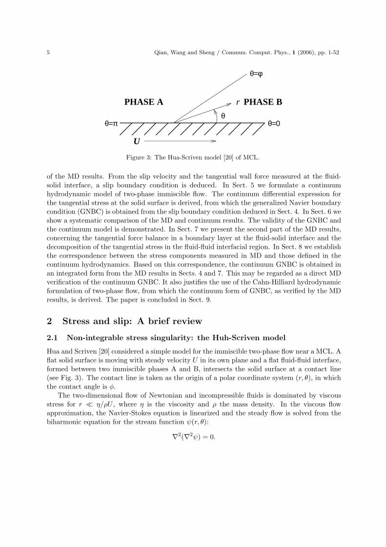
5 Qian, Wang and Sheng / Commun. Comput. Phys., 1 (2006), pp. 1-52
θ=0
PHASE A
θ=φ
θ
r PHASE B
U
θ=π
Figure 3: The Hua-Scriven model [20] of MCL.
of the MD results. From the slip velocity and the tangential wall force measured at the fluid-solid interface, a slip boundary condition is deduced. In Sect. 5 we formulate a continuumhydrodynamic model of two-phase immiscible flow. The continuum differential expression forthe tangential stress at the solid surface is derived, from which the generalized Navier boundarycondition (GNBC) is obtained from the slip boundary condition deduced in Sect. 4. In Sect. 6 weshow a systematic comparison of the MD and continuum results. The validity of the GNBC andthe continuum model is demonstrated. In Sect. 7 we present the second part of the MD results,concerning the tangential force balance in a boundary layer at the fluid-solid interface and thedecomposition of the tangential stress in the fluid-fluid interfacial region. In Sect. 8 we establishthe correspondence between the stress components measured in MD and those defined in thecontinuum hydrodynamics. Based on this correspondence, the continuum GNBC is obtained inan integrated form from the MD results in Sects. 4 and 7. This may be regarded as a direct MDverification of the continuum GNBC. It also justifies the use of the Cahn-Hilliard hydrodynamicformulation of two-phase flow, from which the continuum form of GNBC, as verified by the MDresults, is derived. The paper is concluded in Sect. 9.
2 Stress and slip: A brief review
2.1 Non-integrable stress singularity: the Huh-Scriven model
Hua and Scriven [20] considered a simple model for the immiscible two-phase flow near a MCL. Aflat solid surface is moving with steady velocity U in its own plane and a flat fluid-fluid interface,formed between two immiscible phases A and B, intersects the solid surface at a contact line(see Fig. 3). The contact line is taken as the origin of a polar coordinate system (r, θ), in whichthe contact angle is φ.
The two-dimensional flow of Newtonian and incompressible fluids is dominated by viscousstress for r ¿ η/ρU , where η is the viscosity and ρ the mass density. In the viscous flowapproximation, the Navier-Stokes equation is linearized and the steady flow is solved from thebiharmonic equation for the stream function ψ(r, θ):
∇2(∇2ψ) = 0.
Qian, Wang and Sheng / Commun. Comput. Phys., 1 (2006), pp. 1-52 6
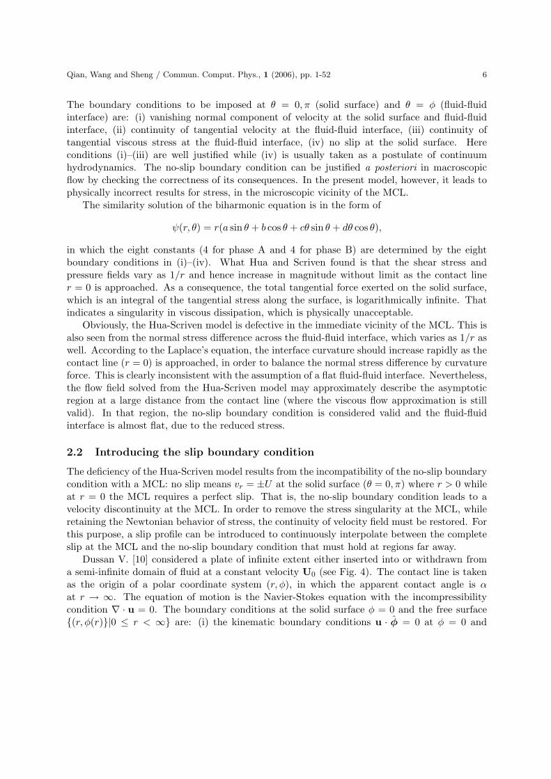
The boundary conditions to be imposed at θ = 0, π (solid surface) and θ = φ (fluid-fluidinterface) are: (i) vanishing normal component of velocity at the solid surface and fluid-fluidinterface, (ii) continuity of tangential velocity at the fluid-fluid interface, (iii) continuity oftangential viscous stress at the fluid-fluid interface, (iv) no slip at the solid surface. Hereconditions (i)–(iii) are well justified while (iv) is usually taken as a postulate of continuumhydrodynamics. The no-slip boundary condition can be justified a posteriori in macroscopicflow by checking the correctness of its consequences. In the present model, however, it leads tophysically incorrect results for stress, in the microscopic vicinity of the MCL.
The similarity solution of the biharmonic equation is in the form of
ψ(r, θ) = r(a sin θ + b cos θ + cθ sin θ + dθ cos θ),
in which the eight constants (4 for phase A and 4 for phase B) are determined by the eightboundary conditions in (i)–(iv). What Hua and Scriven found is that the shear stress andpressure fields vary as 1/r and hence increase in magnitude without limit as the contact liner = 0 is approached. As a consequence, the total tangential force exerted on the solid surface,which is an integral of the tangential stress along the surface, is logarithmically infinite. Thatindicates a singularity in viscous dissipation, which is physically unacceptable.
Obviously, the Hua-Scriven model is defective in the immediate vicinity of the MCL. This isalso seen from the normal stress difference across the fluid-fluid interface, which varies as 1/r aswell. According to the Laplace’s equation, the interface curvature should increase rapidly as thecontact line (r = 0) is approached, in order to balance the normal stress difference by curvatureforce. This is clearly inconsistent with the assumption of a flat fluid-fluid interface. Nevertheless,the flow field solved from the Hua-Scriven model may approximately describe the asymptoticregion at a large distance from the contact line (where the viscous flow approximation is stillvalid). In that region, the no-slip boundary condition is considered valid and the fluid-fluidinterface is almost flat, due to the reduced stress.
2.2 Introducing the slip boundary condition
The deficiency of the Hua-Scriven model results from the incompatibility of the no-slip boundarycondition with a MCL: no slip means vr = ±U at the solid surface (θ = 0, π) where r > 0 whileat r = 0 the MCL requires a perfect slip. That is, the no-slip boundary condition leads to avelocity discontinuity at the MCL. In order to remove the stress singularity at the MCL, whileretaining the Newtonian behavior of stress, the continuity of velocity field must be restored. Forthis purpose, a slip profile can be introduced to continuously interpolate between the completeslip at the MCL and the no-slip boundary condition that must hold at regions far away.
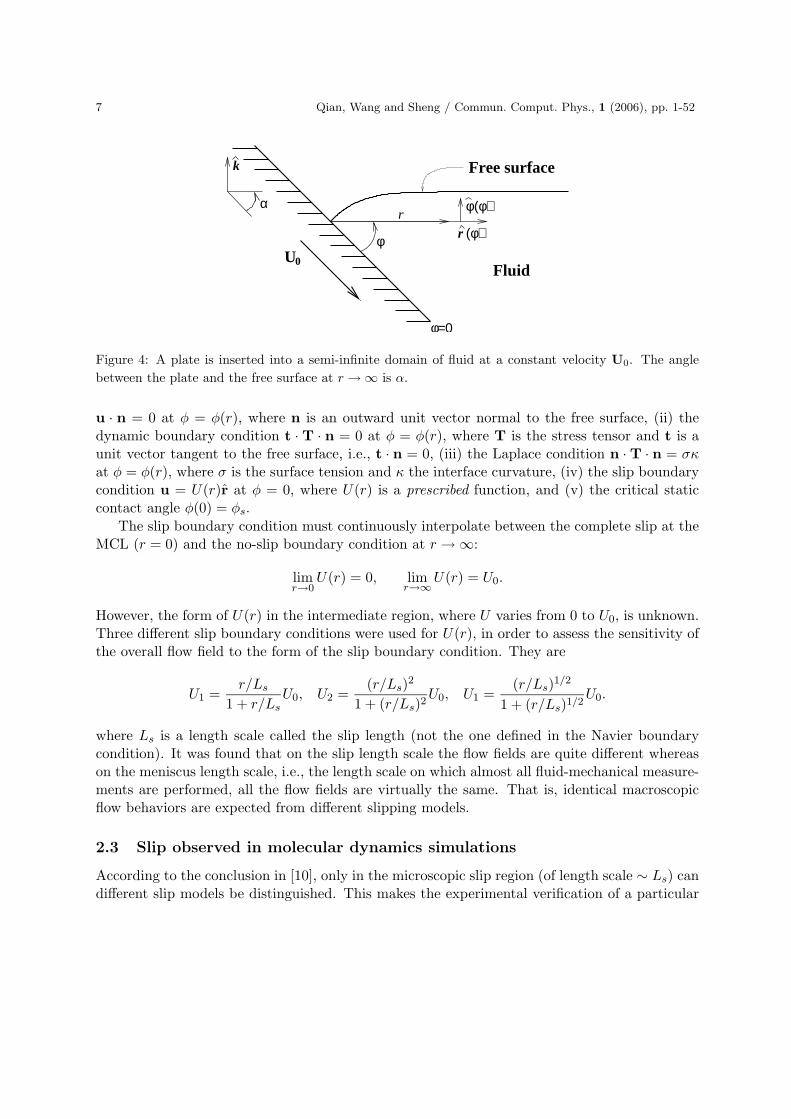
Dussan V. [10] considered a plate of infinite extent either inserted into or withdrawn froma semi-infinite domain of fluid at a constant velocity U0 (see Fig. 4). The contact line is takenas the origin of a polar coordinate system (r, φ), in which the apparent contact angle is αat r → ∞. The equation of motion is the Navier-Stokes equation with the incompressibilitycondition ∇ · u = 0. The boundary conditions at the solid surface φ = 0 and the free surface{(r, φ(r)}|0 ≤ r < ∞} are: (i) the kinematic boundary conditions u · φ = 0 at φ = 0 and
7 Qian, Wang and Sheng / Commun. Comput. Phys., 1 (2006), pp. 1-52
r
φ r (φ)
φ(φ)
Fluid
Free surface
0U
φ=0
α
k
Figure 4: A plate is inserted into a semi-infinite domain of fluid at a constant velocity U0. The angle
between the plate and the free surface at r → ∞ is α.
u · n = 0 at φ = φ(r), where n is an outward unit vector normal to the free surface, (ii) thedynamic boundary condition t · T · n = 0 at φ = φ(r), where T is the stress tensor and t is aunit vector tangent to the free surface, i.e., t · n = 0, (iii) the Laplace condition n · T · n = σκat φ = φ(r), where σ is the surface tension and κ the interface curvature, (iv) the slip boundarycondition u = U(r)r at φ = 0, where U(r) is a prescribed function, and (v) the critical staticcontact angle φ(0) = φs.
The slip boundary condition must continuously interpolate between the complete slip at theMCL (r = 0) and the no-slip boundary condition at r → ∞:
limr→0
U(r) = 0, limr→∞
U(r) = U0.
However, the form of U(r) in the intermediate region, where U varies from 0 to U0, is unknown.Three different slip boundary conditions were used for U(r), in order to assess the sensitivity ofthe overall flow field to the form of the slip boundary condition. They are
U1 =r/Ls
1 + r/LsU0, U2 =
(r/Ls)2
1 + (r/Ls)2U0, U1 =
(r/Ls)1/2
1 + (r/Ls)1/2U0.
where Ls is a length scale called the slip length (not the one defined in the Navier boundarycondition). It was found that on the slip length scale the flow fields are quite different whereason the meniscus length scale, i.e., the length scale on which almost all fluid-mechanical measure-ments are performed, all the flow fields are virtually the same. That is, identical macroscopicflow behaviors are expected from different slipping models.
2.3 Slip observed in molecular dynamics simulations
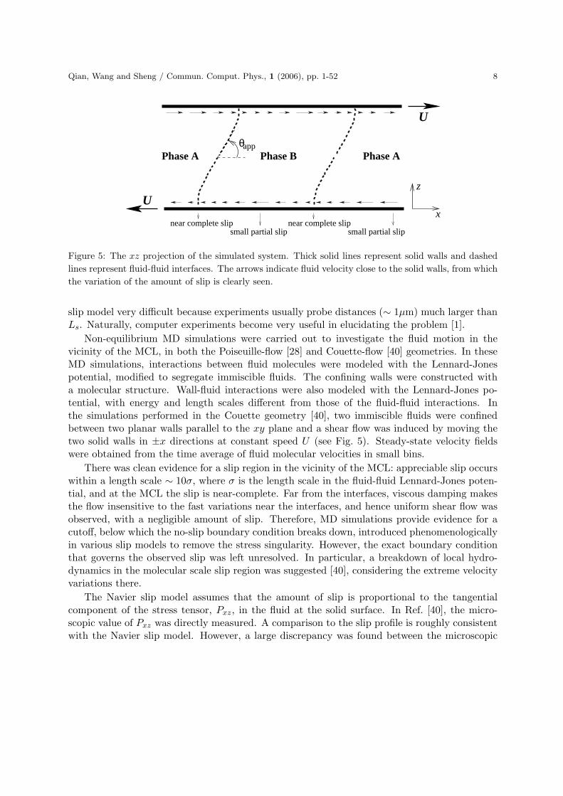
According to the conclusion in [10], only in the microscopic slip region (of length scale ∼ Ls) candifferent slip models be distinguished. This makes the experimental verification of a particular
Qian, Wang and Sheng / Commun. Comput. Phys., 1 (2006), pp. 1-52 8
U
U
Phase B Phase APhase A
near complete slip near complete slipsmall partial slip small partial slip
z
x
θapp
Figure 5: The xz projection of the simulated system. Thick solid lines represent solid walls and dashed
lines represent fluid-fluid interfaces. The arrows indicate fluid velocity close to the solid walls, from which
the variation of the amount of slip is clearly seen.
slip model very difficult because experiments usually probe distances (∼ 1µm) much larger thanLs. Naturally, computer experiments become very useful in elucidating the problem [1].
Non-equilibrium MD simulations were carried out to investigate the fluid motion in thevicinity of the MCL, in both the Poiseuille-flow [28] and Couette-flow [40] geometries. In theseMD simulations, interactions between fluid molecules were modeled with the Lennard-Jonespotential, modified to segregate immiscible fluids. The confining walls were constructed witha molecular structure. Wall-fluid interactions were also modeled with the Lennard-Jones po-tential, with energy and length scales different from those of the fluid-fluid interactions. Inthe simulations performed in the Couette geometry [40], two immiscible fluids were confinedbetween two planar walls parallel to the xy plane and a shear flow was induced by moving thetwo solid walls in ±x directions at constant speed U (see Fig. 5). Steady-state velocity fieldswere obtained from the time average of fluid molecular velocities in small bins.
There was clean evidence for a slip region in the vicinity of the MCL: appreciable slip occurswithin a length scale ∼ 10σ, where σ is the length scale in the fluid-fluid Lennard-Jones poten-tial, and at the MCL the slip is near-complete. Far from the interfaces, viscous damping makesthe flow insensitive to the fast variations near the interfaces, and hence uniform shear flow wasobserved, with a negligible amount of slip. Therefore, MD simulations provide evidence for acutoff, below which the no-slip boundary condition breaks down, introduced phenomenologicallyin various slip models to remove the stress singularity. However, the exact boundary conditionthat governs the observed slip was left unresolved. In particular, a breakdown of local hydro-dynamics in the molecular scale slip region was suggested [40], considering the extreme velocityvariations there.
The Navier slip model assumes that the amount of slip is proportional to the tangentialcomponent of the stress tensor, Pxz, in the fluid at the solid surface. In Ref. [40], the micro-scopic value of Pxz was directly measured. A comparison to the slip profile is roughly consistentwith the Navier slip model. However, a large discrepancy was found between the microscopic
9 Qian, Wang and Sheng / Commun. Comput. Phys., 1 (2006), pp. 1-52
S
fluid 1
L
fluid 2θ
S/1 γ
s1γ s2γ12 S/2
rv
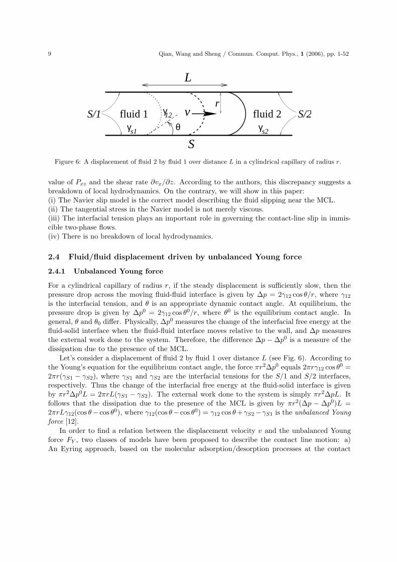
Figure 6: A displacement of fluid 2 by fluid 1 over distance L in a cylindrical capillary of radius r.
value of Pxz and the shear rate ∂vx/∂z. According to the authors, this discrepancy suggests abreakdown of local hydrodynamics. On the contrary, we will show in this paper:(i) The Navier slip model is the correct model describing the fluid slipping near the MCL.(ii) The tangential stress in the Navier model is not merely viscous.(iii) The interfacial tension plays an important role in governing the contact-line slip in immis-cible two-phase flows.(iv) There is no breakdown of local hydrodynamics.
2.4 Fluid/fluid displacement driven by unbalanced Young force
2.4.1 Unbalanced Young force
For a cylindrical capillary of radius r, if the steady displacement is sufficiently slow, then thepressure drop across the moving fluid-fluid interface is given by ∆p = 2γ12 cos θ/r, where γ12
is the interfacial tension, and θ is an appropriate dynamic contact angle. At equilibrium, thepressure drop is given by ∆p0 = 2γ12 cos θ0/r, where θ0 is the equilibrium contact angle. Ingeneral, θ and θ0 differ. Physically, ∆p0 measures the change of the interfacial free energy at thefluid-solid interface when the fluid-fluid interface moves relative to the wall, and ∆p measuresthe external work done to the system. Therefore, the difference ∆p − ∆p0 is a measure of thedissipation due to the presence of the MCL.
Let’s consider a displacement of fluid 2 by fluid 1 over distance L (see Fig. 6). According tothe Young’s equation for the equilibrium contact angle, the force πr2∆p0 equals 2πrγ12 cos θ0 =2πr(γS1 − γS2), where γS1 and γS2 are the interfacial tensions for the S/1 and S/2 interfaces,respectively. Thus the change of the interfacial free energy at the fluid-solid interface is givenby πr2∆p0L = 2πrL(γS1 − γS2). The external work done to the system is simply πr2∆pL. Itfollows that the dissipation due to the presence of the MCL is given by πr2(∆p − ∆p0)L =2πrLγ12(cos θ− cos θ0), where γ12(cos θ− cos θ0) = γ12 cos θ +γS2 −γS1 is the unbalanced Young
force [12].
In order to find a relation between the displacement velocity v and the unbalanced Youngforce FY , two classes of models have been proposed to describe the contact line motion: a)An Eyring approach, based on the molecular adsorption/desorption processes at the contact
Qian, Wang and Sheng / Commun. Comput. Phys., 1 (2006), pp. 1-52 10
xλ
U(a) (b)
W
~F
λ
fluid 1θfluid 2v
ξ
K K−+
Y
2λ
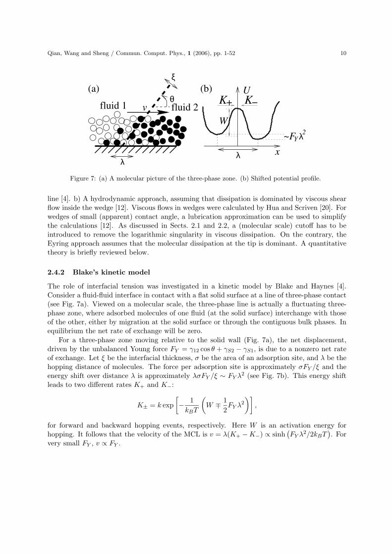
Figure 7: (a) A molecular picture of the three-phase zone. (b) Shifted potential profile.
line [4]. b) A hydrodynamic approach, assuming that dissipation is dominated by viscous shearflow inside the wedge [12]. Viscous flows in wedges were calculated by Hua and Scriven [20]. Forwedges of small (apparent) contact angle, a lubrication approximation can be used to simplifythe calculations [12]. As discussed in Sects. 2.1 and 2.2, a (molecular scale) cutoff has to beintroduced to remove the logarithmic singularity in viscous dissipation. On the contrary, theEyring approach assumes that the molecular dissipation at the tip is dominant. A quantitativetheory is briefly reviewed below.
2.4.2 Blake’s kinetic model
The role of interfacial tension was investigated in a kinetic model by Blake and Haynes [4].Consider a fluid-fluid interface in contact with a flat solid surface at a line of three-phase contact(see Fig. 7a). Viewed on a molecular scale, the three-phase line is actually a fluctuating three-phase zone, where adsorbed molecules of one fluid (at the solid surface) interchange with thoseof the other, either by migration at the solid surface or through the contiguous bulk phases. Inequilibrium the net rate of exchange will be zero.
For a three-phase zone moving relative to the solid wall (Fig. 7a), the net displacement,driven by the unbalanced Young force FY = γ12 cos θ + γS2 − γS1, is due to a nonzero net rateof exchange. Let ξ be the interfacial thickness, σ be the area of an adsorption site, and λ be thehopping distance of molecules. The force per adsorption site is approximately σFY /ξ and theenergy shift over distance λ is approximately λσFY /ξ ∼ FY λ2 (see Fig. 7b). This energy shiftleads to two different rates K+ and K−:
K± = k exp
[
− 1
kBT
(
W ∓ 1
2FY λ2
)]
,
for forward and backward hopping events, respectively. Here W is an activation energy forhopping. It follows that the velocity of the MCL is v = λ(K+ −K−) ∝ sinh
(
FY λ2/2kBT)
. Forvery small FY , v ∝ FY .

11 Qian, Wang and Sheng / Commun. Comput. Phys., 1 (2006), pp. 1-52
x
z0z=z
z=0
Figure 8: A boundary layer of fluid at the fluid-solid interface, responsible for viscous momentum trans-
port between fluid and solid. Circles represent fluid molecules and solid squares represent wall molecules.
Blake’s kinetic model shows that fluid slipping can be induced by the unbalanced Youngforce at the contact line. Therefore, it emphasizes the role of interfacial tension, though not in ahydrodynamic formulation. On the contrary, the authors of Ref. [40] considered the viscous shearstress as the only driving force. In fact a large discrepancy was found between the shear rateand the microscopic value of the tangential stress (the driving force according to the Navier slipmodel). In this paper we will show that in the two-phase interfacial region, such a discrepancyis exactly caused by the neglect of the non-viscous contribution from interfacial tension.
2.5 From the Navier boundary condition to the generalized Navier boundarycondition: a preliminary discussion
Here we give a preliminary account on the main finding reported in Ref. [34], the GNBC. Basedon the results reviewed in Sects. 2.1, 2.2, 2.3, and 2.4, we try to show: a) The Navier boundarycondition may actually work for the single-phase slip region near the MCL. b) In the two-phasecontact-line region, the GNBC is a natural extension of the Navier boundary condition, withthe fluid-fluid interfacial tension taken into account.
2.5.1 Navier boundary condition and slip length
The validity of the Navier boundary condition vslip = −lsn ·[
(∇v) + (∇v)T]
has been wellestablished by many MD studies for single-phase fluids [2, 8, 39, 41]. This boundary conditionis a constitutive equation that locally relates the amount of slip to the shear rate at the solidsurface, though in most of the reported simulations, the hydrodynamics involves no spatialvariation along the solid surface. Physically, the Navier boundary condition is local in naturesimply because intermolecular wall-fluid interactions are short-ranged.
The slip length ls is a phenomenological parameter that measures the local viscous couplingbetween fluid and solid. Fig. 8 illustrates the viscous momentum transport between fluid andsolid through a boundary layer of fluid. The thickness of this boundary layer, z0, must be ofmolecular scale, within the range of wall-fluid interactions. Now we show that the slip length lsis defined based on a linear law for tangential wall force and the Newton’s law for shear stress.
Hydrodynamic motion of fluid at the solid surface is measured by the slip velocity vslipx in
the x direction, defined relative to the (moving) wall. When vslipx is present, a tangential wall
Qian, Wang and Sheng / Commun. Comput. Phys., 1 (2006), pp. 1-52 12
force Gwx is exerted on the boundary-layer fluid, defined as the rate of tangential (x) momentum
transport per unit wall area, from the wall to the (boundary-layer) fluid. Physically, this forcerepresents a time-averaged effect of wall-fluid interactions, to be incorporated into a hydrody-namic slip boundary condition. The linear law for Gw
x is expressed by Gwx = −βvslip, where β is
called the slip coefficient and the minus sign means the fluid-solid coupling is viscous (frictional).For the boundary layer of molecular thickness, the tangential wall force Gw
x must be balancedby the tangential fluid force Gf
x =∫ z0
0 dz (∂xσxx + ∂zσzx), where the integral is over the z-spanof the boundary layer (see Fig. 8), σxx(zx) are the xx(zx) components of the fluid stress tensor,and ∂xσxx + ∂zσzx is the fluid force density in the x direction. From the equation of tangentialforce balance Gw
x + Gfx = 0, we obtain
∫ z0
0dz (∂xσxx + ∂zσzx) = ∂x
∫ z0
0dzσxx(x, z) + σzx(x, z0) = βvslip(x).
This equation should be regarded as a microscopic expression for the Navier slip model: theamount of slip is proportional to the tangential fluid force at the fluid-solid interface. When thenormal stress σxx varies slowly in the x direction and the tangential stress σzx is caused by shearviscosity only, the above equation becomes η∂zvx(x, z0) = βvslip(x), where η is the viscosity and∂zvx(x, z0) is the shear rate “at the solid surface”. For flow fields whose characteristic lengthscale is much larger than z0, the boundary layer thickness, we replace z0 by z = 0 and recover theNavier boundary condition for continuum hydrodynamics, in which the slip length is given byls = η/β. To summarize, the hydrodynamic viscous coupling between fluid and solid is actuallymeasured by the slip coefficient β. The Navier boundary condition, in which the slip length isintroduced, is due to the Newton’s law for viscous shear stress. For very weak viscous couplingbetween fluid and solid, β → 0, and thus ls → ∞, making ∂zvx → 0: the fluid-solid interfacebecomes a free surface.
2.5.2 Single-phase region
A number of MD studies have shown that for single-phase flows, the Navier boundary conditionis valid in describing the fluid slipping at solid surface [2, 8, 39, 41]. Therefore, we expect thatit can also describe the partial slip observed in the single-phase region near the MCL [40].However, according to the authors of Ref. [40], the Navier boundary condition failed even inthe single-phase region: the velocity gradient ∂vx/∂z was not proportional to the amount ofslip. This discrepancy was attributed to a breakdown of local hydrodynamics, considering thevery large velocity variations observed near the MCL. Here we present a heuristic discussion,to explain why such a discrepancy is expected even if the Navier boundary condition actuallyworks for the single-phase region.
First, the success of the hybrid approaches outlined below strongly indicates that localhydrodynamics doesn’t break down in the slip region. In Ref. [40], an apparent contact angleθapp was defined at half the distance between two solid surfaces (see Fig. 5). For θapp < 135◦,fluid-fluid interfaces could be approximated by planes. The Navier-Stokes equation was solvedfor the simplified geometry. For this purpose, the tangential velocity along fluid-fluid interface

13 Qian, Wang and Sheng / Commun. Comput. Phys., 1 (2006), pp. 1-52
θ =π/2app
no−slip condition
Navier−Stokes equation
x
z
vNavier condition
x
O U
Figure 9: Two-dimensional corner flow caused by one rigid plane sliding over another, with constant
inclination θapp = 90◦. In the reference frame of the vertical plane, the horizontal plane is moving to the
left with constant speed U .
was set to be zero (according to the simulation results) and the slip velocity ∆V (r) (measuredrelative to the moving wall) was specified as a function of distance r from the MCL: ∆V (r) =±U exp[−r ln 2/S], with + and − for the lower and upper walls, respectively. This ∆V (r),proposed according to the MD slip profile, continuously interpolates between the complete slipat the MCL (∆V (r) = ±U at r = 0) and the no-slip boundary condition (∆V (r) → 0 atr → ∞). With a proper value chosen for S (≈ 1.8σ), the MD flow fields were reproduced bysolving the Navier-Stokes equation with the above boundary conditions. Recently, an improvedhybrid approach has been used to reproduce the MD simulation results for contact-line motionin a Poiseuille geometry [15].
To further test the validity of continuum modeling, we have solved the Navier-Stokes equationfor a corner flow [33]. Consider one rigid plane sliding steadily over another, with constantinclination θapp (see Fig. 9). The fluid is Newtonian and incompressible. The no-slip boundarycondition is applied at the vertical plane and the Navier boundary condition applied at thehorizontal plane. The kinematic condition of vanishing normal component of velocity at thesolid surface requires vx = 0 at the vertical plane and vz = 0 at the horizontal plane, andhence v = 0 at the intersection O, which is taken as the origin of the coordinate system (x, z).This corner-flow model resembles the continuum model used in the hybrid approach above, andproduces similar flow fields for quantitative comparison with MD results. In particular, thecorner flow exhibits a slip profile very close to ∆V (r): the slip velocity vx + U shows a lineardecrease over a length scale ∼ ls, the slip length in the Navier condition, followed by a moregradual decrease. (Note that vx + U = U at O implies complete slip.)
From the hybrid approach with the prescribed slip velocity ∆V (r) to the corner-flow modelwith the Navier boundary condition, they indicate that the single-phase region near the MCLcan be modeled by the Navier-Stokes equation for an incompressible Newtonian fluid, supple-mented by appropriate boundary conditions. Then a simple question arises: Given a continuumhydrodynamic model that uses the Navier boundary condition and approximately reproduces
Qian, Wang and Sheng / Commun. Comput. Phys., 1 (2006), pp. 1-52 14
the MD flow fields in the single-phase region near the MCL, why do the MD simulation resultsshow a large discrepancy between the velocity gradient ∂vx/∂z and the amount of slip?
The answer lies in the fast velocity variation in the vicinity of the MCL, where the flow isdominated by viscous stress. With the characteristic velocity scale set by U and the characteristiclength scale set by ls, the normal stress σxx must show as well a fast variation along the solidsurface: ∂xσxx ∼ ηU/l2s . According to Sect. 2.5.1, the microscopic value of the tangential fluid
force Gfx is given by ∂x
∫ z0
0 dzσxx(x, z) + σzx(x, z0). This expression is necessary because Gfx
is distributed in a boundary layer of molecular thickness z0. Obviously, to represent Gfx by
σzx ≈ η∂vx/∂z at z = z0 alone, the normal stress σxx near the solid surface has to vary slowlyin the x direction. This is not the case in the vicinity of the MCL if the Navier slip modelworks there, as implied by the continuum corner-flow calculation which yields ∂xσxx ∼ ηU/l2snear the intersection. (It is reasonable to expect that if the Navier slip model is valid, then thenormal stress measured in MD simulations should in general agree with that from continuummodel calculation with the Navier condition.) Given ∂x
∫ z0
0 dzσxx ∼ ηUz0/l2s according to thecorner-flow model, and that z0 and ls are both ∼ 1σ, it is obvious that considering only η∂vx/∂z
at z = z0 would lead to an appreciable underestimate of Gfx ∼ ηU/ls in the slip region. In short,
the large discrepancy between the velocity gradient ∂vx/∂z and the amount of slip, observed inthe single-phase slip region near the MCL, cannot be used to exclude the microscopic Navier slipmodel and the hydrodynamic Navier slip boundary condition, for if the Navier model is valid,then the tangential viscous stress η∂vx/∂z, measured at some level away from the solid surface,
is not enough for a complete evaluation of the tangential fluid force Gfx.
2.5.3 Two-phase region
The linear law for tangential wall force, Gwx = −βvslip
x , describes the hydrodynamic viscouscoupling between fluid and solid. Assume that in the two-phase region, the two fluids interactwith the wall independently. Then the tangential wall force becomes Gw
x = −βvslipx at the
contact line, with the slip coefficient given by β = (β1ρ1 + β2ρ2)/(ρ1 + ρ2), where β1 and β2 arethe slip coefficients for the two single-phase regions separated by the fluid-fluid interface, andρ1 and ρ2 are the local densities of the two fluids in the contact-line region. Obviously, β variesbetween β1 and β2 across the fluid-fluid interface.
The equation of tangential force balance Gwx + Gf
x = 0 must hold as well in the two-phaseregion. Therefore the Navier slip model is still of the form
∂x
∫ z0
0dzσxx(x, z) + σzx(x, z0) = βvslip(x).
Nevertheless, this does not lead to the Navier boundary condition η∂zvx = βvslip anymorebecause in the two-phase region, the tangential stress is not contributed by shear viscosity only:there is a non-viscous component in σzx, caused by the fluid-fluid interfacial tension. Put in anideal form of decomposition, the tangential stress σzx(x, z) at level z can be expressed as
σzx(x, z) = σvzx(x, z) + σY
zx(x, z),
15 Qian, Wang and Sheng / Commun. Comput. Phys., 1 (2006), pp. 1-52
where σvzx is the viscous component due to shear viscosity and σY
zx (the tangential Young stress) isthe non-viscous component, which is narrowly distributed in the two-phase interfacial region andrelated to the interfacial tension through
∫
int dxσYzx(x, z) = γ cos θ(z). Here
∫
int dx denotes theintegration across the fluid-fluid interface along the x direction, γ is the interfacial tension, andθ(z) is the angle between the interface and the x direction at level z. Physically, the existence ofa fluid-fluid interface causes an anisotropy in the stress tensor in the two-phase interfacial region.The interfacial tension is an integrated measure of that stress anisotropy. When expressed in acoordinate system different from the principal system, the stress tensor is not diagonalized and anonzero σY
zx appears. In the presence of shear flow, while the shear viscosity leads to the viscouscomponent σv
zx in σzx, the non-viscous component σYzx is still present. A detailed discussion on
the stress decomposition will be given in Sect. 7.3.Consider an equilibrium state in which the tangential stress σ0
zx is balanced by the gradientof the normal stress σ0
xx:
∂x
∫ z0
0dzσ0
xx(x, z) + σ0zx(x, z0) = 0,
where the superscript 0 denotes equilibrium quantities. Here the equilibrium tangential stressσ0
zx is narrowly distributed in the two-phase interfacial region and related to the interfacialtension through
∫
int dxσ0zx(x, z) = γ cos θ0(z). (There is no viscous stress in equilibrium, and
hence σ0zx is caused by the interfacial tension only.) Subtracting the equation of equilibrium
force balance from the expression of Navier slip model, we obtain
∂x
∫ z0
0dz[σxx(x, z) − σ0
xx(x, z)] + [σzx(x, z0) − σ0zx(x, z0)]
= ∂x
∫ z0
0dz[σxx(x, z) − σ0
xx(x, z)] + [σvzx(x, z0) + σY
zx(x, z0) − σ0zx(x, z0)]
= βvslip(x).
This equation will be the focus of our continuum deduction from molecular hydrodynamics.In fact it leads to the GNBC which governs the fluid slipping everywhere, from the two-phasecontact-line region to the single-phase regions away from the MCL. This will be elaborated inSects. 4, 5, 7, and 8.
To summarize, our preliminary analysis shows that compared to the single-phase regionwhere the tangential stress is due to shear viscosity only, the two-phase region has the tangentialYoung stress as the additional component. Naturally, the Navier boundary condition, whichconsiders the tangential viscous stress only, needs to be generalized to include the tangentialYoung stress.
3 Statement of results
We have carried out MD simulations for immiscible two-phase flows in a Couette geometry (seeFig. 10) [34]. The two immiscible fluids were modeled by using the Lennard-Jones (LJ) potentialsfor the interactions between fluid molecules. The solid walls were modeled by crystalline plates.
Qian, Wang and Sheng / Commun. Comput. Phys., 1 (2006), pp. 1-52 16
V
V
x
z
y
H
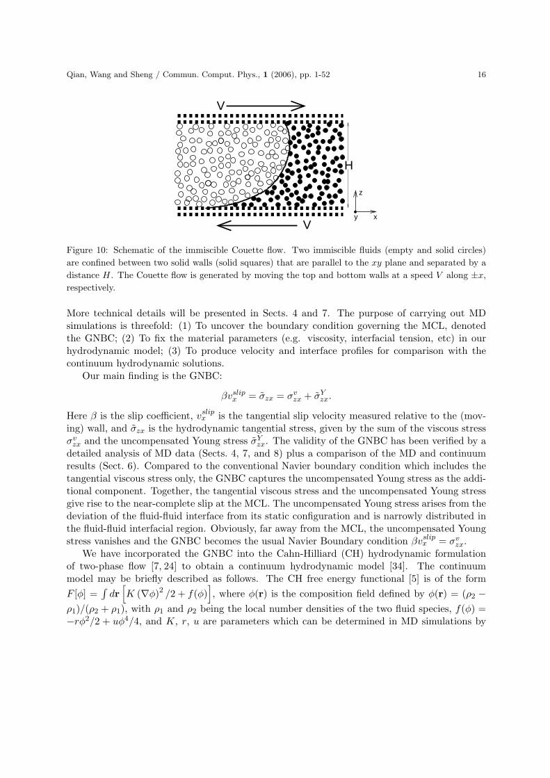
Figure 10: Schematic of the immiscible Couette flow. Two immiscible fluids (empty and solid circles)
are confined between two solid walls (solid squares) that are parallel to the xy plane and separated by a
distance H. The Couette flow is generated by moving the top and bottom walls at a speed V along ±x,
respectively.
More technical details will be presented in Sects. 4 and 7. The purpose of carrying out MDsimulations is threefold: (1) To uncover the boundary condition governing the MCL, denotedthe GNBC; (2) To fix the material parameters (e.g. viscosity, interfacial tension, etc) in ourhydrodynamic model; (3) To produce velocity and interface profiles for comparison with thecontinuum hydrodynamic solutions.
Our main finding is the GNBC:
βvslipx = σzx = σv
zx + σYzx.
Here β is the slip coefficient, vslipx is the tangential slip velocity measured relative to the (mov-
ing) wall, and σzx is the hydrodynamic tangential stress, given by the sum of the viscous stressσv
zx and the uncompensated Young stress σYzx. The validity of the GNBC has been verified by a
detailed analysis of MD data (Sects. 4, 7, and 8) plus a comparison of the MD and continuumresults (Sect. 6). Compared to the conventional Navier boundary condition which includes thetangential viscous stress only, the GNBC captures the uncompensated Young stress as the addi-tional component. Together, the tangential viscous stress and the uncompensated Young stressgive rise to the near-complete slip at the MCL. The uncompensated Young stress arises from thedeviation of the fluid-fluid interface from its static configuration and is narrowly distributed inthe fluid-fluid interfacial region. Obviously, far away from the MCL, the uncompensated Youngstress vanishes and the GNBC becomes the usual Navier Boundary condition βvslip
x = σvzx.
We have incorporated the GNBC into the Cahn-Hilliard (CH) hydrodynamic formulationof two-phase flow [7, 24] to obtain a continuum hydrodynamic model [34]. The continuummodel may be briefly described as follows. The CH free energy functional [5] is of the form
F [φ] =∫
dr[
K (∇φ)2 /2 + f(φ)]
, where φ(r) is the composition field defined by φ(r) = (ρ2 −ρ1)/(ρ2 + ρ1), with ρ1 and ρ2 being the local number densities of the two fluid species, f(φ) =−rφ2/2 + uφ4/4, and K, r, u are parameters which can be determined in MD simulations by
17 Qian, Wang and Sheng / Commun. Comput. Phys., 1 (2006), pp. 1-52
measuring the interface width ξ =√
K/r, the interfacial tension γ = 2√
2r2ξ/3u, and the twohomogeneous equilibrium phases φ± = ±
√
r/u (= ±1 in our case). The two coupled equationsof motion are the CH convection-diffusion equation for φ and the Navier-Stokes equation (withthe addition of the capillary force density):
∂φ
∂t+ v · ∇φ = M∇2µ, (3.1)
ρm
[
∂v
∂t+ (v · ∇)v
]
= −∇p + ∇ · σv + µ∇φ + mρgext, (3.2)
together with the incompressibility condition ∇·v = 0. Here M is the phenomenological mobilitycoefficient, ρm is the fluid mass density, p is the pressure, σv is the Newtonian viscous stresstensor, µ∇φ is the capillary force density with µ = δF/δφ being the chemical potential, andmρgext is the external body force density (for Poiseuille flows). The boundary conditions atthe solid surface are vn = 0, ∂nµ = 0 (n denotes the outward surface normal), a relaxationalequation for φ at the solid surface:
∂φ
∂t+ v · ∇φ = −ΓL(φ), (3.3)
and the continuum form of the GNBC:
βvslipx = −η∂nvx + L(φ)∂xφ, (3.4)
Here Γ is a (positive) phenomenological parameter, L(φ) = K∂nφ + ∂γwf (φ)/∂φ with γwf (φ)
being the fluid-solid interfacial free energy density, β is the slip coefficient, vslipx is the (tangential)
slip velocity relative to the wall, η is the viscosity, and L(φ)∂xφ is the uncompensated Youngstress.
Compared to the Navier boundary condition, the additional component captured by theGNBC in Eq. (3.4) is the uncompensated Young stress σY
zx. Its differential expression is givenby
σYzx = L(φ)∂xφ = [K∂nφ + ∂γwf (φ)/∂φ]∂xφ (3.5)
at z = 0. Here the z coordinate is for the lower fluid-solid interface where ∂n = −∂z (samebelow), with the understanding that the same physics holds at the upper interface. It canbe shown that the integral of this uncompensated Young stress along x across the fluid-fluidinterface yields
∫
intdx[L(φ)∂xφ](x, 0) = γ cos θsurf
d + ∆γwf , (3.6)
where∫
int dx denotes the integration along x across the fluid-fluid interface, γ is the fluid-fluid
interfacial tension, θsurfd is the dynamic contact angle at the solid surface, and ∆γwf is the
change of γwf (φ) across the fluid-fluid interface, i.e., ∆γwf ≡∫
int dx∂xγwf (φ). The Young’s
equation relates ∆γwf to the static contact angle θsurfs at the solid surface:
γ cos θsurfs + ∆γwf = 0, (3.7)
Qian, Wang and Sheng / Commun. Comput. Phys., 1 (2006), pp. 1-52 18
which is obtained as a phenomenological expression for the tangential force balance at the contactline in equilibrium. Substituting Eq. (3.7) into Eq. (3.6) yields
∫
intdx[L(φ)∂xφ](x, 0) = γ(cos θsurf
d − cos θsurfs ), (3.8)
implying that the uncompensated Young stress arises from the deviation of the fluid-fluid in-terface from its static configuration. Equations (3.5), (3.6), (3.7), and (3.8) will be derived inSect. 5. In essence, our results show that in the vicinity of the MCL, the tangential viscousstress −η∂nvx as postulated by the usual Navier boundary condition can not account for thecontact-line slip profile without taking into account the uncompensated Young stress. This isseen from both the MD data and the predictions of the continuum model.
Besides the external conditions such as the shear speed V and the wall separation H, thereare nine parameters in our continuum model, including ρm, η, β, ξ, γ, |φ±|, M , Γ, and θsurf
s .
The values of ρm, η, β, ξ, γ, |φ±|, and θsurfs were directly obtained from MD simulations. The
values of the two phenomenological parameters M and Γ were fixed by an optimized comparisonwith one MD flow field. The same set of parameters (corresponding to the same local propertiesin a series of MD simulations) has been used to produce velocity fields and fluid-fluid interfaceshapes for comparison with the MD results obtained for different external conditions (V , H,and flow geometry). The overall agreement is excellent in all cases, demonstrating the validityof the GNBC and the hydrodynamic model.
The CH hydrodynamic formulation of immiscible two-phase flow has been successfully used toconstruct a continuum model. We would like to emphasize that while the phase-field formulationdoes provide a convenient way of modeling that is familiar to us, it should not be conceived asthe unique way. After all, what we need is to incorporate our key finding, the GNBC, into acontinuum formulation of immiscible two-phase flow. The GNBC itself is simply a fact found inMD simulations, independent of any continuum formulation.
4 Molecular Dynamics I
4.1 Geometry and interactions
MD simulations have been carried out for two-phase immiscible flows in Couette geometry (seeFigs. 10 and 11) [34]. Two immiscible fluids were confined between two planar solid wallsparallel to the xy plane, with the fluid-solid boundaries defined by z = 0, H. The Couetteflow was generated by moving the top and bottom walls at a constant speed V in the ±xdirections, respectively. Periodic boundary conditions were imposed along the x and y directions.Interaction between fluid molecules separated by a distance r was modeled by a modified LJpotential
Uff = 4ε[
(σ/r)12 − δff (σ/r)6]
,
where ε is the energy scale, σ is the range scale, with δff = 1 for like molecules and δff = −1for molecules of different species. (The negative δff was used to ensure immiscibility.) The
19 Qian, Wang and Sheng / Commun. Comput. Phys., 1 (2006), pp. 1-52
average number density for the fluids was set at ρ = 0.81σ−3. The temperature was controlledat 2.8ε/kB. (This high temperature was used to reduce the near-surface layering induced bythe solid wall.) Each wall was constructed by two [001] planes of an fcc lattice, with each wallmolecule attached to a lattice site by a harmonic spring. The mass of the wall molecule was setequal to that of the fluid molecule m. The number density of the wall was set at ρw = 1.86σ−3.The wall-fluid interaction was modeled by another LJ potential
Uwf = 4εwf
[
(σwf/r)12 − δwf (σwf/r)6]
,
with the energy and range parameters given by εwf = 1.16ε and σwf = 1.04σ, and δwf forspecifying the wetting property of the fluid. There is no locked layer of fluid molecules at thesolid surface. We have considered two cases. In the symmetric case, the two fluids have theidentical wall-fluid interactions with δwf = 1. Consequently, the static contact angle is 90◦ andthe fluid-fluid interface is flat, parallel to the yz plane. In the asymmetric case, the two fluidshave different wall-fluid interactions, with δwf = 1 for one and δwf = 0.7 for the other. Asa consequence, the static contact angle is 64◦ and the fluid-fluid interface is curved in the xzplane. In most of our simulations, the shearing speed V was on the order of 0.1
√
ε/m, the sampledimension along y was 6.8σ, the wall separation along z varied from H = 6.8σ to 68σ, and thesample dimension along x was set to be long enough so that the uniform single-fluid shear flowwas recovered far away from the MCL. Steady-state quantities were obtained from time averageover 105τ or longer where τ is the atomic time scale
√
mσ2/ε. Throughout the remainder ofthis paper, all physical quantities are given in terms of the LJ reduced units (defined in termsof ε, σ, and m).
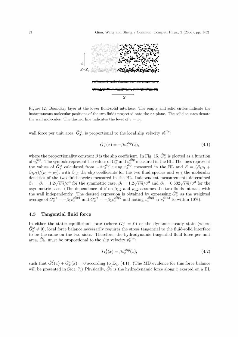
4.2 Boundary-layer tangential wall force
We denote the region within z0 = 0.85σ from the wall the boundary layer (BL) (see Fig. 12).It must be thin enough to ensure sufficient precision for measuring the slip velocity at the solidsurface, but also thick enough to fully account for the tangential wall-fluid interaction force,which is of a finite range. The wall force can be singled out by separating the force on each fluidmolecule into wall-fluid and fluid-fluid components. The fluid molecules in the BL, being closeto the solid wall, can experience a strong periodic modulation in interaction with the wall. Thislateral inhomogeneity is generally referred to as the “roughness” of the wall potential [41]. Whencoupled with kinetic collisions with the wall molecules, there arises a nonzero tangential wall forcedensity gw
x that is sharply peaked at z ≈ z0/2 and vanishes beyond z ≈ z0 (see Fig. 13). Fromthe force density gw
x , we define the tangential wall force per unit area as Gwx (x) =
∫ z0
0 dzgwx (x, z),
which is the total tangential wall force accumulated across the BL.The short saturation range of the tangential wall force may be understood as follows. Out
of the BL, each fluid molecule can interact with many wall molecules on a nearly equal basis.Thus the modulation amplitude (the roughness) of the wall potential would clearly decreasewith increasing distance from the wall. That’s why the tangential wall force tends to saturateat z ≈ z0, which is still within the cutoff distance of wall-fluid interaction. On the contrary, thenormal wall force arises from the direct wall-fluid interaction, independent of whether the wall
Qian, Wang and Sheng / Commun. Comput. Phys., 1 (2006), pp. 1-52 20
symmetric asymmetric
fluid 2fluid 1 fluid 1 fluid 1 fluid 2 fluid 1
(a)
x
y
z
V
V
fluid 2 fluid 1fluid 1
(b)
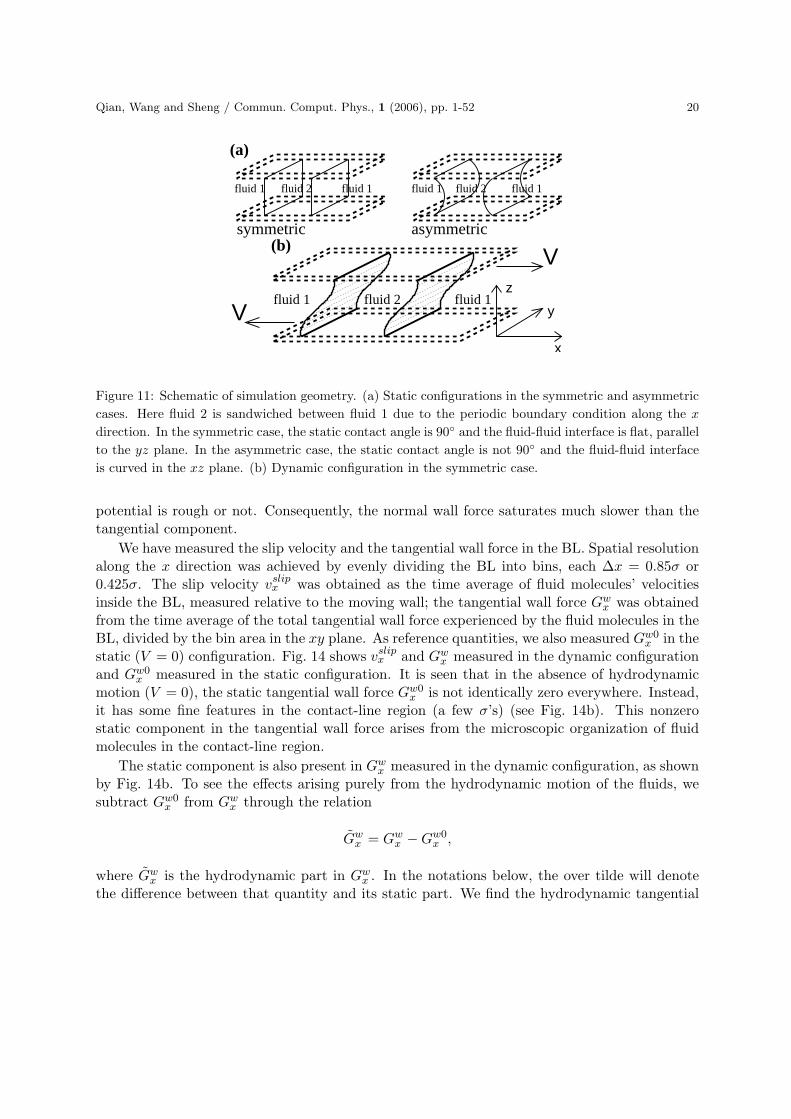
Figure 11: Schematic of simulation geometry. (a) Static configurations in the symmetric and asymmetric
cases. Here fluid 2 is sandwiched between fluid 1 due to the periodic boundary condition along the x
direction. In the symmetric case, the static contact angle is 90◦ and the fluid-fluid interface is flat, parallel
to the yz plane. In the asymmetric case, the static contact angle is not 90◦ and the fluid-fluid interface
is curved in the xz plane. (b) Dynamic configuration in the symmetric case.
potential is rough or not. Consequently, the normal wall force saturates much slower than thetangential component.
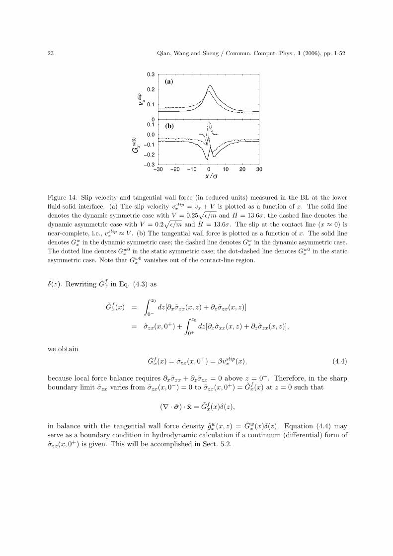
We have measured the slip velocity and the tangential wall force in the BL. Spatial resolutionalong the x direction was achieved by evenly dividing the BL into bins, each ∆x = 0.85σ or0.425σ. The slip velocity vslip
x was obtained as the time average of fluid molecules’ velocitiesinside the BL, measured relative to the moving wall; the tangential wall force Gw
x was obtainedfrom the time average of the total tangential wall force experienced by the fluid molecules in theBL, divided by the bin area in the xy plane. As reference quantities, we also measured Gw0
x in thestatic (V = 0) configuration. Fig. 14 shows vslip
x and Gwx measured in the dynamic configuration
and Gw0x measured in the static configuration. It is seen that in the absence of hydrodynamic
motion (V = 0), the static tangential wall force Gw0x is not identically zero everywhere. Instead,
it has some fine features in the contact-line region (a few σ’s) (see Fig. 14b). This nonzerostatic component in the tangential wall force arises from the microscopic organization of fluidmolecules in the contact-line region.
The static component is also present in Gwx measured in the dynamic configuration, as shown
by Fig. 14b. To see the effects arising purely from the hydrodynamic motion of the fluids, wesubtract Gw0
x from Gwx through the relation
Gwx = Gw
x − Gw0x ,
where Gwx is the hydrodynamic part in Gw
x . In the notations below, the over tilde will denotethe difference between that quantity and its static part. We find the hydrodynamic tangential
21 Qian, Wang and Sheng / Commun. Comput. Phys., 1 (2006), pp. 1-52
x
z=z0
z
Figure 12: Boundary layer at the lower fluid-solid interface. The empty and solid circles indicate the
instantaneous molecular positions of the two fluids projected onto the xz plane. The solid squares denote
the wall molecules. The dashed line indicates the level of z = z0.
wall force per unit area, Gwx , is proportional to the local slip velocity vslip
x :
Gwx (x) = −βvslip
x (x), (4.1)
where the proportionality constant β is the slip coefficient. In Fig. 15, Gwx is plotted as a function
of vslipx . The symbols represent the values of Gw
x and vslipx measured in the BL. The lines represent
the values of Gwx calculated from −βvslip
x using vslipx measured in the BL and β = (β1ρ1 +
β2ρ2)/(ρ1 + ρ2), with β1,2 the slip coefficients for the two fluid species and ρ1,2 the moleculardensities of the two fluid species measured in the BL. Independent measurements determinedβ1 = β2 = 1.2
√εm/σ3 for the symmetric case, β1 = 1.2
√εm/σ3 and β2 = 0.532
√εm/σ3 for the
asymmetric case. (The dependence of β on β1,2 and ρ1,2 assumes the two fluids interact withthe wall independently. The desired expression is obtained by expressing Gw
x as the weightedaverage of Gw1
x = −β1vslip1x and Gw2
x = −β2vslip2x and noting vslip1
x ≈ vslip2x to within 10%).
4.3 Tangential fluid force
In either the static equilibrium state (where Gwx = 0) or the dynamic steady state (where
Gwx 6= 0), local force balance necessarily requires the stress tangential to the fluid-solid interface
to be the same on the two sides. Therefore, the hydrodynamic tangential fluid force per unitarea, Gf
x, must be proportional to the slip velocity vslipx :
Gfx(x) = βvslip
x (x), (4.2)
such that Gfx(x) + Gw
x (x) = 0 according to Eq. (4.1). (The MD evidence for this force balance
will be presented in Sect. 7.) Physically, Gfx is the hydrodynamic force along x exerted on a BL
Qian, Wang and Sheng / Commun. Comput. Phys., 1 (2006), pp. 1-52 22
0 0.2 0.4 0.6 0.8 1
z /
0
2
4
6
8
gxw(z
) / Gxw (
)
σ
σ−1
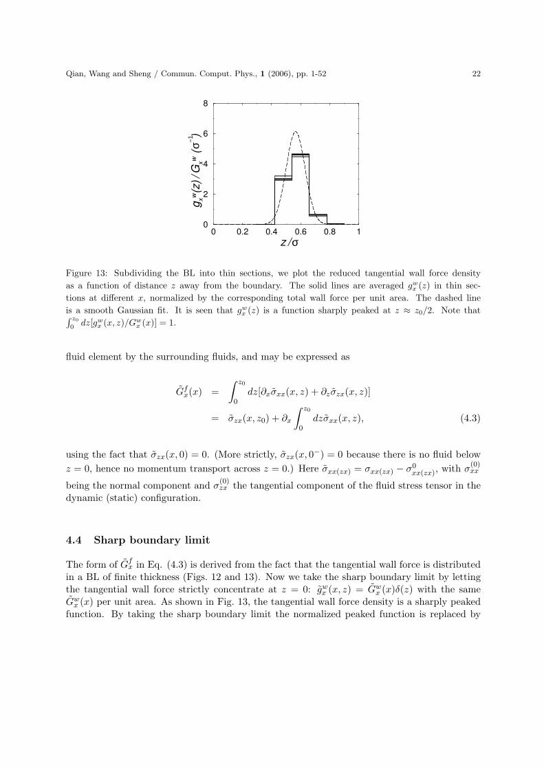
Figure 13: Subdividing the BL into thin sections, we plot the reduced tangential wall force density
as a function of distance z away from the boundary. The solid lines are averaged gwx (z) in thin sec-
tions at different x, normalized by the corresponding total wall force per unit area. The dashed line
is a smooth Gaussian fit. It is seen that gwx (z) is a function sharply peaked at z ≈ z0/2. Note that
∫ z0
0dz[gw
x (x, z)/Gwx (x)] = 1.
fluid element by the surrounding fluids, and may be expressed as
Gfx(x) =
∫ z0
0dz[∂xσxx(x, z) + ∂zσzx(x, z)]
= σzx(x, z0) + ∂x
∫ z0
0dzσxx(x, z), (4.3)
using the fact that σzx(x, 0) = 0. (More strictly, σzx(x, 0−) = 0 because there is no fluid below
z = 0, hence no momentum transport across z = 0.) Here σxx(zx) = σxx(zx) − σ0xx(zx), with σ
(0)xx
being the normal component and σ(0)zx the tangential component of the fluid stress tensor in the
dynamic (static) configuration.
4.4 Sharp boundary limit
The form of Gfx in Eq. (4.3) is derived from the fact that the tangential wall force is distributed
in a BL of finite thickness (Figs. 12 and 13). Now we take the sharp boundary limit by lettingthe tangential wall force strictly concentrate at z = 0: gw
x (x, z) = Gwx (x)δ(z) with the same
Gwx (x) per unit area. As shown in Fig. 13, the tangential wall force density is a sharply peaked
function. By taking the sharp boundary limit the normalized peaked function is replaced by
23 Qian, Wang and Sheng / Commun. Comput. Phys., 1 (2006), pp. 1-52
−30 −20 −10 0 10 20 30
x /
−0.3
−0.2
−0.1
0.0
0.1
Gxw
(0)
0
0.1
0.2
0.3
vxslip
σ
(a)
(b)
Figure 14: Slip velocity and tangential wall force (in reduced units) measured in the BL at the lower
fluid-solid interface. (a) The slip velocity vslipx = vx + V is plotted as a function of x. The solid line
denotes the dynamic symmetric case with V = 0.25√
ε/m and H = 13.6σ; the dashed line denotes the
dynamic asymmetric case with V = 0.2√
ε/m and H = 13.6σ. The slip at the contact line (x ≈ 0) is
near-complete, i.e., vslipx ≈ V . (b) The tangential wall force is plotted as a function of x. The solid line
denotes Gwx in the dynamic symmetric case; the dashed line denotes Gw
x in the dynamic asymmetric case.
The dotted line denotes Gw0x in the static symmetric case; the dot-dashed line denotes Gw0
x in the static
asymmetric case. Note that Gw0x vanishes out of the contact-line region.
δ(z). Rewriting Gfx in Eq. (4.3) as
Gfx(x) =
∫ z0
0−dz[∂xσxx(x, z) + ∂zσzx(x, z)]
= σzx(x, 0+) +
∫ z0
0+
dz[∂xσxx(x, z) + ∂zσzx(x, z)],
we obtain
Gfx(x) = σzx(x, 0+) = βvslip
x (x), (4.4)
because local force balance requires ∂xσxx + ∂zσzx = 0 above z = 0+. Therefore, in the sharpboundary limit σzx varies from σzx(x, 0−) = 0 to σzx(x, 0+) = Gf
x(x) at z = 0 such that
(∇ · σ) · x = Gfx(x)δ(z),
in balance with the tangential wall force density gwx (x, z) = Gw
x (x)δ(z). Equation (4.4) mayserve as a boundary condition in hydrodynamic calculation if a continuum (differential) form ofσzx(x, 0+) is given. This will be accomplished in Sect. 5.2.
Qian, Wang and Sheng / Commun. Comput. Phys., 1 (2006), pp. 1-52 24
−20 −10 0 10 20
1 / v
xslip
−30
−20
−10
0
10
20
30
1 / G
xw
~
Figure 15: 1/Gwx plotted as a function of 1/vslip
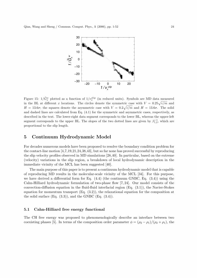
x (in reduced units). Symbols are MD data measured
in the BL at different x locations. The circles denote the symmetric case with V = 0.25√
ε/m and
H = 13.6σ; the squares denote the asymmetric case with V = 0.2√
ε/m and H = 13.6σ. The solid
and dashed lines are calculated from Eq. (4.1) for the symmetric and asymmetric cases, respectively, as
described in the text. The lower-right data segment corresponds to the lower BL, whereas the upper-left
segment corresponds to the upper BL. The slopes of the two dotted lines are given by β−11,2 , which are
proportional to the slip length.
5 Continuum Hydrodynamic Model
For decades numerous models have been proposed to resolve the boundary condition problem forthe contact-line motion [4,7,19,21,24,38,43], but so far none has proved successful by reproducingthe slip velocity profiles observed in MD simulations [28,40]. In particular, based on the extreme(velocity) variations in the slip region, a breakdown of local hydrodynamic description in theimmediate vicinity of the MCL has been suggested [40].
The main purpose of this paper is to present a continuum hydrodynamic model that is capableof reproducing MD results in the molecular-scale vicinity of the MCL [34]. For this purpose,we have derived a differential form for Eq. (4.4) (the continuum GNBC, Eq. (3.4)) using theCahn-Hilliard hydrodynamic formulation of two-phase flow [7, 24]. Our model consists of theconvection-diffusion equation in the fluid-fluid interfacial region (Eq. (3.1)), the Navier-Stokesequation for momentum transport (Eq. (3.2)), the relaxational equation for the composition atthe solid surface (Eq. (3.3)), and the GNBC (Eq. (3.4)).
5.1 Cahn-Hilliard free energy functional
The CH free energy was proposed to phenomenologically describe an interface between twocoexisting phases [5]. In terms of the composition order parameter φ = (ρ2 − ρ1)/(ρ2 + ρ1), the
25 Qian, Wang and Sheng / Commun. Comput. Phys., 1 (2006), pp. 1-52
CH free energy functional reads
F =
∫
dr
[
1
2K (∇φ)2 + f(φ)
]
,
with f(φ) = −12rφ2 + 1
4uφ4. Two thermally stable phases are given by φ± = ±√
r/u at which∂f/∂φ = 0. An interface can be formed between the phases of φ+ and φ− in coexistence.
5.1.1 Chemical potential
The chemical potential µ is defined by
µ =δF
δφ= −K∇2φ − rφ + uφ3,
from which the diffusion current J = −M∇µ is obtained with M being the mobility coefficient.The convection-diffusion equation (Eq. (3.1)) comes from the continuity equation
Dφ
Dt=
∂φ
∂t+ v · ∇φ = −∇ · J.
5.1.2 Interfacial tension
A few important physical quantities can be derived from the CH free energy. We first derive theinterfacial tension γ for the interface formed between φ+ and φ−. In equilibrium, the spatialvariation of φ is determined by the condition that µ(r) is constant, i.e.,
−K∂2zφ − rφ + uφ3 = constant.
Here the interface is assumed to be in the xy plane with the interface normal along the z directionand the constant equals to zero because limz→±∞ φ = φ± and limz→±∞ µ = 0. The interfacialprofile is solved to be
φ0(z) = φ+ tanhz√2ξ
,
with ξ =√
K/r being a characteristic length along the interface normal. The first integral is
−1
2K (∂zφ)2 + f(φ) = C,
where the integral constant C equals f(φ±). It follows the interfacial free energy per unit area,i.e., the interfacial tension, is given by
γ =
∫
dz
[
1
2K (∂zφ)2 + f(φ) − f(φ±)
]
=
∫
dzK (∂zφ)2 .
Using the interfacial profile φ0(z), we obtain
γ =Kφ2
±√2ξ
∫
dz cosh−4 z =2√
2Kφ2±
3ξ=
2√
2r2ξ
3u.
Qian, Wang and Sheng / Commun. Comput. Phys., 1 (2006), pp. 1-52 26
5.1.3 Capillary force and Young stress
We now turn to the forces arising from the interface. Consider a virtual displacement u(r) andthe corresponding variation in φ, δφ(r) = −u(r) · ∇φ. The change of the free energy due to thisδφ is
δF =
∫
dr
[
∂f(φ)
∂φδφ
]
+
∫
dr
∂[
12K (∇φ)2
]
∂(∂jφ)δ (∂jφ)
=
∫
dr [µδφ] +
∫
ds [K∂nφδφ]
= −∫
dr [g · u] +
∫
ds[
σYniui
]
,
where g = µ∇φ is the capillary force density in the Navier-Stokes equation (Eq. (3.2)), andσY
ni = −K∂nφ∂iφ is the tangential Young stress (the i direction is along the fluid-solid interface,i ⊥ n).
The body force g(r) = µ∇φ can be reduced to the familiar curvature force in the sharpinterface limit [6]. The unit vector normal to the level sets of constant φ is given by m = ∇φ/|∇φ|and
µ∇φ = [−K∇2φ − rφ + uφ3]|∇φ|m= −K∇2
t φ|∇φ|m + [−K∂2mφ − rφ + uφ3]|∇φ|m
where ∇t and ∂m denote the differentiations tangential and normal to the interface respectively.For gently curved interfaces, the order parameter φ along the interface normal can be approx-imated by the one-dimensional stationary solution φ0, i.e., −K∂2
mφ − rφ + uφ3 ≈ 0. Hence,µ∇φ ≈ −K∇2
t φ|∇φ|m, from which we obtain the desired relation
µ∇φ ≈ K|∇φ|2κm ≈ γκδ(lm)m,
where κ = −∇2t φ/|∇φ| is the curvature and γ ≈
∫
dlmK (∇φ)2 ≈∫
dlmK (∂mφ)2 is the interfa-cial tension, with lm being the coordinate along the interface normal and the interface locatedat lm = 0.
For gently curved interfaces, K∂nφ ≈ K∂mφ cos θsurf , where n is the outward (solid) surfacenormal, m the (fluid-fluid) interface normal, and θsurf the angle at which the interface intersectsthe solid surface (n · m = cos θsurf ). For the tangential Young stress σY
zx = K∂nφ∂xφ atz = 0 where n = −z and i = x, the integral
∫
int dxσYzx along x across the interface equals
to∫
int dxK∂nφ∂xφ = (∫
int dφK∂mφ) cos θsurf , where∫
int dφK∂mφ =∫
int dlmK (∂mφ)2 = γ.Hence,
∫
intdxσY
zx = γ cos θsurf , (5.1)
where θsurf may be the dynamic contact angle at the solid surface θsurfd or the static contact
angle θsurfs . This
∫
int dxσYzx is the tangential force per unit length at the contact line (aligned
along y), exerted by the fluid-fluid interface of tension γ, which intersects the solid wall at thecontact angle θsurf . So it equals to γ cos θsurf .
27 Qian, Wang and Sheng / Commun. Comput. Phys., 1 (2006), pp. 1-52
5.1.4 Young’s equation
The Young’s equation for the static contact angle θsurfs can be derived as well. Consider the
interfacial free energy at the fluid-solid interface, Fwf =∫
dsγwf (φ). Minimizing the total freeenergy F + Fwf with respect to φ at the solid surface yields
[
K∂nφ +∂γwf (φ)
∂φ
]
φeq
= 0, (5.2)
from which an equation of local tangential force balance[
σYzx
]
φeq
=[
σYzx + ∂xγwf (φ)
]
φeq
= σ0zx + ∂xγwf (φeq) = 0, (5.3)
is obtained at z = 0. Here σYzx = σY
zx+∂xγwf is the uncompensated Young stress (first introducedin Eq. (3.5)), φeq is the equilibrium composition field, and σ0
zx denotes the static Young stressσY
zx(φeq). Integrating Eq. (5.3) along x across the interface leads to the Young’s equation
γ cos θsurfs + ∆γwf = 0 (Eq. (3.7)), where γ cos θsurf
s =∫
int dxσ0zx and ∆γwf ≡
∫
int dx∂xγwf (φ)is the change of fluid-solid interfacial free energy per unit area across the fluid-fluid interface.A microscopic picture for the Young’s equation as an (integrated) equation of tangential forcebalance will be elaborated in Sect. 7.2.1.
5.2 Two boundary conditions
Equations (5.2) and (5.3) are boundary conditions for the equilibrium state. In the dynamicsteady state, however, neither K∂nφ + ∂γwf (φ)/∂φ = L(φ) nor σY
zx + ∂xγwf (φ) = L(φ)∂xφvanishes. In fact, the nonzero L(φ) is responsible for the relaxation of φ at the solid surfacewhile the nonzero L(φ)∂xφ is necessary to a slip boundary condition that is able to account forthe near-complete slip at the MCL.
The convection-diffusion equation (Eq. (3.1)) is fourth-order in space. Consequently, besidesthe usual impermeability condition ∂nµ = 0, one more boundary condition is needed. Thedynamics of φ at the solid surface is plausibly assumed to be relaxational, governed by thefirst-order extension of Eq. (5.2). More explicitly, when the system is driven away from theequilibrium, both ∂φ/∂t + v · ∇φ and L(φ) become nonzero, and they are related to each otherby a linear relation
∂φ
∂t+ v · ∇φ ∝ L(φ).
This leads to Eq. (3.3) with Γ introduced as a phenomenological parameter.The GNBC (Eq. (3.4)) is obtained by substituting
σzx(x, 0+) = σzx(x, 0) − σ0zx(x, 0) = σv
zx(x, 0) + σYzx(x, 0) − σ0
zx(x, 0)= σv
zx(x, 0) + σYzx(x, 0) + ∂xγwf
= σvzx(x, 0) + σY
zx.(5.4)
into Eq. (4.4). Here the hydrodynamic tangential stress σzx is decomposed into a viscouscomponent σv
zx and a non-viscous component σYzx. The viscous component is simply given by
Qian, Wang and Sheng / Commun. Comput. Phys., 1 (2006), pp. 1-52 28
σvzx = η∂zvx; the non-viscous component is the uncompensated Young stress σY
zx, given byσY
zx = σYzx + ∂xγwf (φ) (Eq. (3.5)). According to Eq. (5.3), this uncompensated Young stress
vanishes in the equilibrium state. But in a dynamic configuration, from the integral of σYzx along
x across the fluid-fluid interface (Eqs. (3.6), (3.7), and (3.8))∫
intdxσY
zx = γ cos θsurfd + ∆γwf = γ(cos θsurf
d − cos θsurfs ),
there is always a non-viscous contribution to the total tangential stress σzx as long as the fluid-fluid interface deviates from its static configuration.
In Sect. 6 we will show that the GNBC, with the uncompensated Young stress included, canaccount for the slip velocity profiles in the vicinity of the MCL, especially the near-completeslip at the contact line. In Sects. 7.2 and 7.3 we will present more MD evidence supporting theGNBC. A “derivation” of the GNBC, based on the tangential force balance (Sect. 7.2) and thetangential stress decomposition (Sect. 7.3), will be given in Sect. 8.
5.3 Dimensionless equations
Dimensionless equations suitable for numerical computation are obtained as follows. We scaleφ by |φ±| =
√
r/u, length by ξ =√
K/r, velocity by the wall speed V , time by ξ/V , andpressure/stress by ηV/ξ. In dimensionless forms, the convection-diffusion equation is
∂φ
∂t+ v · ∇φ = Ld∇2(−∇2φ − φ + φ3), (5.5)
the Navier-Stokes equation is
R[
∂v
∂t+ (v · ∇)v
]
= −∇p + ∇2v + B(−∇2φ − φ + φ3)∇φ, (5.6)
the relaxational equation for φ at the solid surface is
∂φ
∂t+ vx∂xφ = −Vs
[
∂nφ −√
2
3cos θsurf
s sγ(φ)
]
, (5.7)
and the GNBC is
[Ls(φ)]−1 vslipx = B
[
∂nφ −√
2
3cos θsurf
s sγ(φ)
]
∂xφ − ∂nvx. (5.8)
Here sγ(φ) = (π/2) cos(πφ/2) is from the fluid-solid interfacial free energy
γwf (φ) = (∆γwf/2) sin(πφ/2),
which denotes a smooth interpolation between ±∆γwf/2. Five dimensionless parameters appearin the above equations. They are (1) Ld = Mr/V ξ, which is the ratio of a diffusion length Mr/Vto ξ, (2) R = ρV ξ/η, (3) B = r2ξ/uηV = 3γ/2
√2ηV , which is inversely proportional to the
capillary number Ca = ηV/γ, (4) Vs = KΓ/V , and (5) Ls(φ) = η/β(φ)ξ, which is the ratioof the slip length ls(φ) = η/β(φ) to ξ, where β(φ) = (1 − φ)β1/2 + (1 + φ)β2/2. A numericalalgorithm based on a fixed uniform mesh has been presented in Ref. [34].
29 Qian, Wang and Sheng / Commun. Comput. Phys., 1 (2006), pp. 1-52
6 Comparison of MD and continuum results
To demonstrate the validity of our continuum model, we have obtained numerical solutions thatcan be directly compared to the MD results for flow field and fluid-fluid interface shape. We havecarried out the MD-continuum comparison in such a way that virtually no adjustable parameteris involved in the continuum calculations. This is achieved as follows.
There are totally nine material parameters in our continuum model. They are ρm, η, β, ξ, γ,|φ±|, M , Γ, and θsurf
s . (Note (1) For the asymmetric case, two unequal slip coefficients β1 and β2
are involved in β; (2) The three parameters ξ, γ, and |φ±| are equivalent to the three parameters
K, r, and u in the CH free energy density; (3) θsurfs is for ∆γwf = −γ cos θsurf
s .) Among thenine parameters, seven are directly obtainable (measurable) in MD simulations. They are ρm,
η, β1,2, ξ, γ, |φ±|, and θsurfs . (The fluid mass density ρm is set in MD simulations, the viscosity
η and the slip coefficients β1,2 can be measured in suitable single-fluid MD simulations, the in-terfacial thickness ξ can be obtained by measuring the interfacial profile φ = (ρ2 − ρ1)/(ρ2 + ρ1)in MD simulations, the interfacial tension γ can be obtained by measuring an integral of thepressure/stress anisotropy in the interfacial region [26], |φ±| = 1 means the total immiscibility of
the two fluids, and the static contact angle θsurfs is directly measurable.) The two phenomeno-
logical parameters M and Γ have been introduced to describe the composition dynamics in theinterfacial region. Their values are fixed by an optimized MD-continuum comparison. Thatis, one MD flow field is best matched by varying the continuum flow field with respect to thevalues of M and Γ. Once all the parameter values are obtained (7 measured in MD simulationsand 2 fixed by one MD-continuum comparison), our continuum hydrodynamic model can yieldpredictions that can be readily compared to the results from a series of MD simulations withdifferent external conditions (V , H, and flow geometry). The overall agreement is excellentin all cases, thus demonstrating the validity of the GNBC and the hydrodynamic model. Weemphasize that the MD-continuum agreement has been achieved both in the molecular-scalevicinity of the contact line and far way from the contact line. This opens up the possibility ofnot only continuum simulations of nano- and microfluidics involving immiscible components, butalso macroscopic immiscible flow calculations that are physically meaningful at the molecularlevel. (Molecular-scale details may be resolved through the iterative grid redistribution methodwithout significantly compromising computation efficiency, see [35,37]).
6.1 Immiscible Couette flow
6.1.1 Two symmetric cases
In Figs. 16 and 17 we show the MD and continuum velocity fields for two symmetric cases ofimmiscible Couette flow. In MD simulations, these two cases have the same local properties (fluiddensity, temperature, fluid-fluid interaction, wall-fluid interaction, etc) but different externalconditions (H and V ). Correspondingly, the continuum results are obtained using the same set
of nine material parameters ρm, η, β (= β1 = β2), ξ, γ, |φ±|, M , Γ, and θsurfs .
Qian, Wang and Sheng / Commun. Comput. Phys., 1 (2006), pp. 1-52 30
6.1.2 Two asymmetric cases
In Figs. 18 and 19 we show the MD and continuum velocity fields for two asymmetric cases ofimmiscible Couette flow. In MD simulations, these two cases have the same local properties (fluiddensity, temperature, fluid-fluid interaction, wall-fluid interaction, etc) but different externalconditions (H and V ). Correspondingly, the continuum results are obtained using the same set
of ten material parameters ρm, η, β1, β2, ξ, γ, |φ±|, M , Γ, and θsurfs . In particular, among these
parameters, β2 and θsurfs are measured in MD simulations while all the others directly come
from the symmetric cases. Therefore, the comparison here is without adjustable parameters.
6.1.3 From near-complete slip to uniform shear flow
From Figs. 16, 17, 18, and 19, we see that at the MCL, the slip is near-complete, i.e., vx ≈ 0and |vslip
x | ≈ V , while far away from the contact line, the flow field is not perturbed by thefluid-fluid interface and the single-fluid uniform shear flow is recovered. The slip amount inthe uniform shear flow is 2lsV/(H + 2ls), vanishing in the limit of H À ls. Here we encounteran intriguing question: In a mesoscopic or macroscopic system, what is the slip profile whichconsistently interpolates between the near-complete slip at the MCL and the no-slip boundarycondition that must hold at regions far away? Large-scale MD and continuum simulations havebeen carried out to answer this question [35].
6.1.4 Steady-state fluid-fluid interface
In Fig. 20 we show the MD and continuum fluid-fluid interface profiles for one symmetric andone asymmetric cases whose velocity fields are shown in Figs. 16 and 18.
6.2 Immiscible Poiseuille flow
In order to further verify that the continuum model is local and the parameter values are localproperties, hence applicable to different flow geometries, we have carried out MD simulationsand continuum calculations for immiscible Poiseuille flows. We find that the continuum modelwith the same set of parameters is capable of reproducing the MD results for velocity field andfluid-fluid interface profile, shown in Fig. 21. Similar to what we have observed in Couette flows,here at the MCL the slip is near-complete, i.e., vx ≈ 0 and |vslip
x | ≈ V , while far away fromthe contact line, the flow field is not perturbed by the fluid-fluid interface and the single-fluidunidirectional Poiseuille flow is recovered. In particular, the slip amount in the unidirectionalPoiseuille flow vanishes in the limit of H À ls.
We emphasize that the overall agreement is excellent in all cases (from Fig. 16 to 21),therefore the validity of the GNBC and the hydrodynamic model is well affirmed.
6.3 Flow in narrow channels
It is generally believed that continuum hydrodynamic predictions tend to deviate more fromthe “true” MD results as the channel is further narrowed [42]. This tendency has indeed been
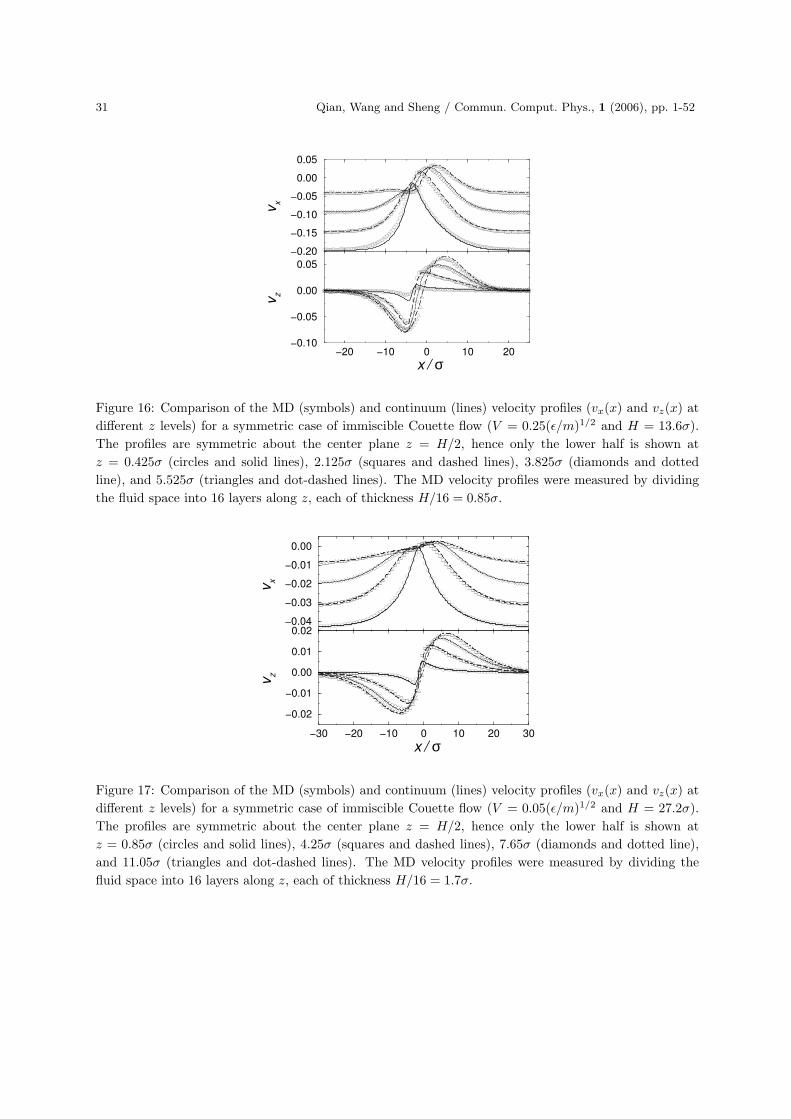
31 Qian, Wang and Sheng / Commun. Comput. Phys., 1 (2006), pp. 1-52
−20 −10 0 10 20
x /
−0.10
−0.05
0.00
0.05v
z
−0.20
−0.15
−0.10
−0.05
0.00
0.05
vx
σ
Figure 16: Comparison of the MD (symbols) and continuum (lines) velocity profiles (vx(x) and vz(x) at
different z levels) for a symmetric case of immiscible Couette flow (V = 0.25(ε/m)1/2 and H = 13.6σ).
The profiles are symmetric about the center plane z = H/2, hence only the lower half is shown at
z = 0.425σ (circles and solid lines), 2.125σ (squares and dashed lines), 3.825σ (diamonds and dotted
line), and 5.525σ (triangles and dot-dashed lines). The MD velocity profiles were measured by dividing
the fluid space into 16 layers along z, each of thickness H/16 = 0.85σ.
−30 −20 −10 0 10 20 30
x /
−0.02
−0.01
0.00
0.01
0.02
vz
−0.04
−0.03
−0.02
−0.01
0.00
vx
σ
Figure 17: Comparison of the MD (symbols) and continuum (lines) velocity profiles (vx(x) and vz(x) at
different z levels) for a symmetric case of immiscible Couette flow (V = 0.05(ε/m)1/2 and H = 27.2σ).
The profiles are symmetric about the center plane z = H/2, hence only the lower half is shown at
z = 0.85σ (circles and solid lines), 4.25σ (squares and dashed lines), 7.65σ (diamonds and dotted line),
and 11.05σ (triangles and dot-dashed lines). The MD velocity profiles were measured by dividing the
fluid space into 16 layers along z, each of thickness H/16 = 1.7σ.
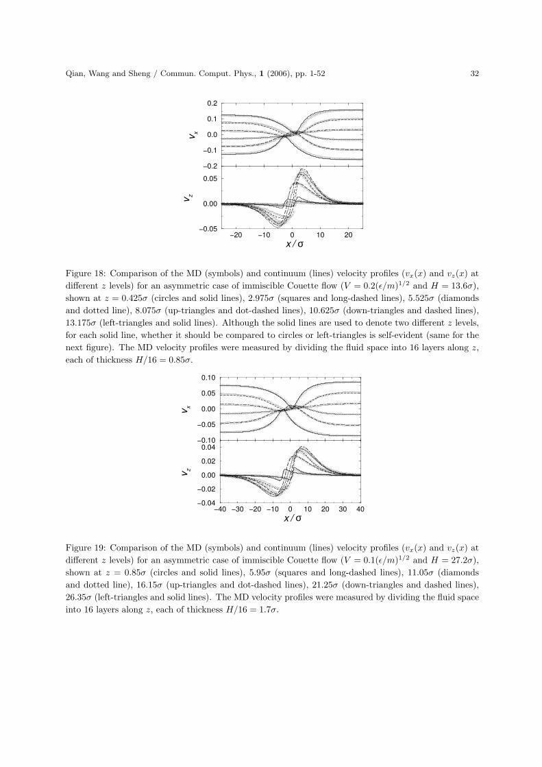
Qian, Wang and Sheng / Commun. Comput. Phys., 1 (2006), pp. 1-52 32
−0.2
−0.1
0.0
0.1
0.2
vx
−20 −10 0 10 20
x /
−0.05
0.00
0.05v
z
σ
Figure 18: Comparison of the MD (symbols) and continuum (lines) velocity profiles (vx(x) and vz(x) at
different z levels) for an asymmetric case of immiscible Couette flow (V = 0.2(ε/m)1/2 and H = 13.6σ),
shown at z = 0.425σ (circles and solid lines), 2.975σ (squares and long-dashed lines), 5.525σ (diamonds
and dotted line), 8.075σ (up-triangles and dot-dashed lines), 10.625σ (down-triangles and dashed lines),
13.175σ (left-triangles and solid lines). Although the solid lines are used to denote two different z levels,
for each solid line, whether it should be compared to circles or left-triangles is self-evident (same for the
next figure). The MD velocity profiles were measured by dividing the fluid space into 16 layers along z,
each of thickness H/16 = 0.85σ.
−40 −30 −20 −10 0 10 20 30 40
x /
−0.04
−0.02
0.00
0.02
0.04
vz
−0.10
−0.05
0.00
0.05
0.10
vx
σ
Figure 19: Comparison of the MD (symbols) and continuum (lines) velocity profiles (vx(x) and vz(x) at
different z levels) for an asymmetric case of immiscible Couette flow (V = 0.1(ε/m)1/2 and H = 27.2σ),
shown at z = 0.85σ (circles and solid lines), 5.95σ (squares and long-dashed lines), 11.05σ (diamonds
and dotted line), 16.15σ (up-triangles and dot-dashed lines), 21.25σ (down-triangles and dashed lines),
26.35σ (left-triangles and solid lines). The MD velocity profiles were measured by dividing the fluid space
into 16 layers along z, each of thickness H/16 = 1.7σ.
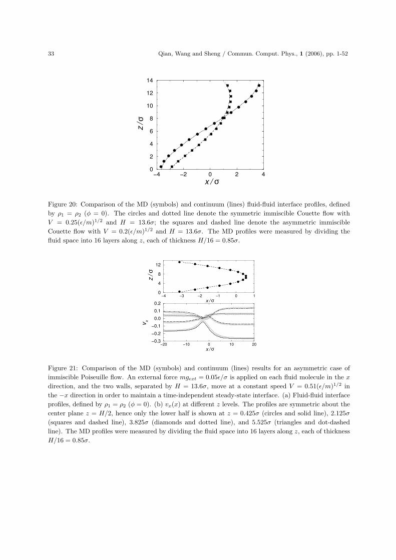
33 Qian, Wang and Sheng / Commun. Comput. Phys., 1 (2006), pp. 1-52
−4 −2 0 2 4
x /
0
2
4
6
8
10
12
14
z /
σ
σ
Figure 20: Comparison of the MD (symbols) and continuum (lines) fluid-fluid interface profiles, defined
by ρ1 = ρ2 (φ = 0). The circles and dotted line denote the symmetric immiscible Couette flow with
V = 0.25(ε/m)1/2 and H = 13.6σ; the squares and dashed line denote the asymmetric immiscible
Couette flow with V = 0.2(ε/m)1/2 and H = 13.6σ. The MD profiles were measured by dividing the
fluid space into 16 layers along z, each of thickness H/16 = 0.85σ.
−20 −10 0 10 20
x /
−0.3
−0.2
−0.1
0.0
0.1
0.2
vx
−4 −3 −2 −1 0 1
x /
0
4
8
12
z /
σ
σ
σ
Figure 21: Comparison of the MD (symbols) and continuum (lines) results for an asymmetric case of
immiscible Poiseuille flow. An external force mgext = 0.05ε/σ is applied on each fluid molecule in the x
direction, and the two walls, separated by H = 13.6σ, move at a constant speed V = 0.51(ε/m)1/2 in
the −x direction in order to maintain a time-independent steady-state interface. (a) Fluid-fluid interface
profiles, defined by ρ1 = ρ2 (φ = 0). (b) vx(x) at different z levels. The profiles are symmetric about the
center plane z = H/2, hence only the lower half is shown at z = 0.425σ (circles and solid line), 2.125σ
(squares and dashed line), 3.825σ (diamonds and dotted line), and 5.525σ (triangles and dot-dashed
line). The MD profiles were measured by dividing the fluid space into 16 layers along z, each of thickness
H/16 = 0.85σ.
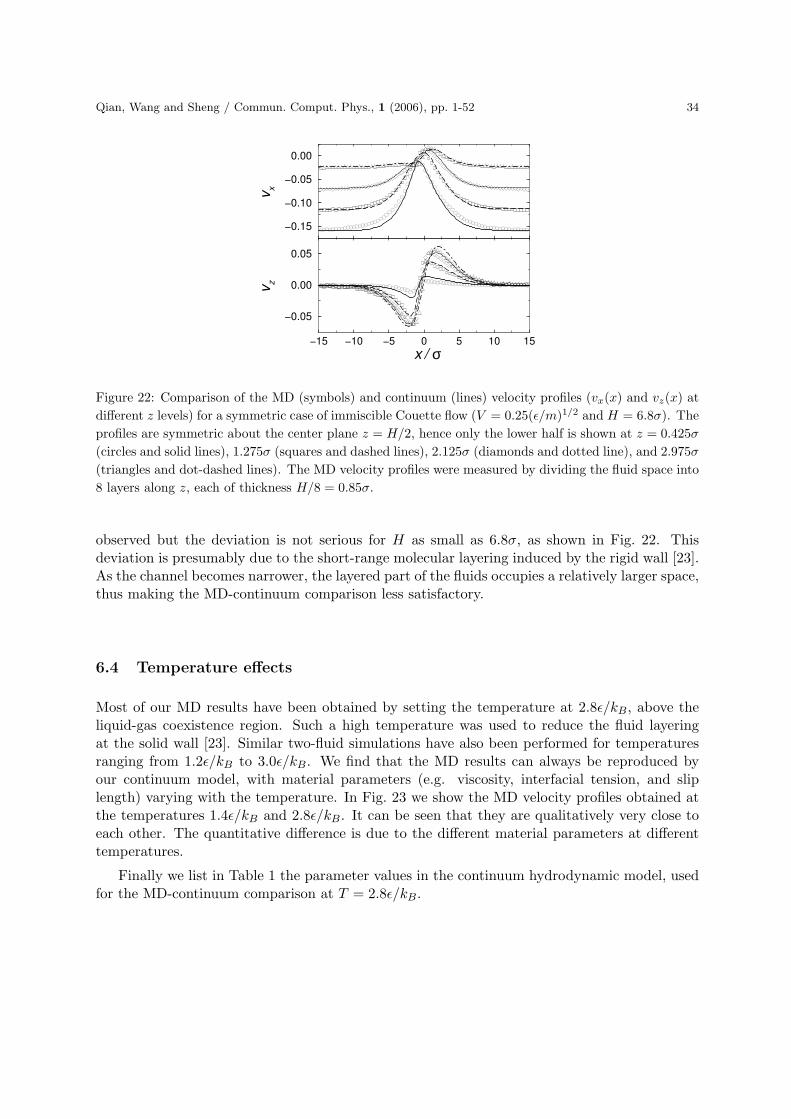
Qian, Wang and Sheng / Commun. Comput. Phys., 1 (2006), pp. 1-52 34
−15 −10 −5 0 5 10 15
x /
−0.05
0.00
0.05v
z
−0.15
−0.10
−0.05
0.00
vx
σ
Figure 22: Comparison of the MD (symbols) and continuum (lines) velocity profiles (vx(x) and vz(x) at
different z levels) for a symmetric case of immiscible Couette flow (V = 0.25(ε/m)1/2 and H = 6.8σ). The
profiles are symmetric about the center plane z = H/2, hence only the lower half is shown at z = 0.425σ
(circles and solid lines), 1.275σ (squares and dashed lines), 2.125σ (diamonds and dotted line), and 2.975σ
(triangles and dot-dashed lines). The MD velocity profiles were measured by dividing the fluid space into
8 layers along z, each of thickness H/8 = 0.85σ.
observed but the deviation is not serious for H as small as 6.8σ, as shown in Fig. 22. Thisdeviation is presumably due to the short-range molecular layering induced by the rigid wall [23].As the channel becomes narrower, the layered part of the fluids occupies a relatively larger space,thus making the MD-continuum comparison less satisfactory.
6.4 Temperature effects
Most of our MD results have been obtained by setting the temperature at 2.8ε/kB, above theliquid-gas coexistence region. Such a high temperature was used to reduce the fluid layeringat the solid wall [23]. Similar two-fluid simulations have also been performed for temperaturesranging from 1.2ε/kB to 3.0ε/kB. We find that the MD results can always be reproduced byour continuum model, with material parameters (e.g. viscosity, interfacial tension, and sliplength) varying with the temperature. In Fig. 23 we show the MD velocity profiles obtained atthe temperatures 1.4ε/kB and 2.8ε/kB. It can be seen that they are qualitatively very close toeach other. The quantitative difference is due to the different material parameters at differenttemperatures.
Finally we list in Table 1 the parameter values in the continuum hydrodynamic model, usedfor the MD-continuum comparison at T = 2.8ε/kB.
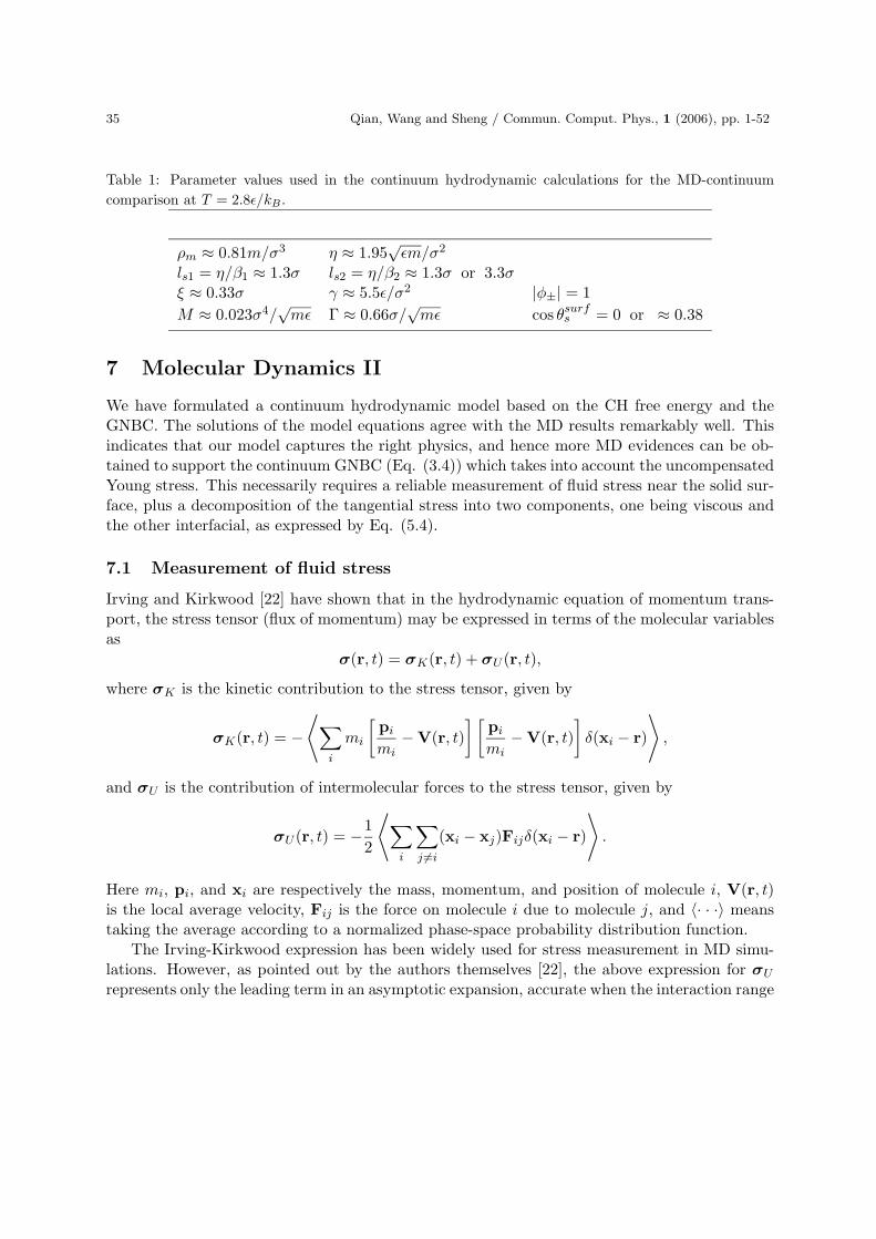
35 Qian, Wang and Sheng / Commun. Comput. Phys., 1 (2006), pp. 1-52
Table 1: Parameter values used in the continuum hydrodynamic calculations for the MD-continuum
comparison at T = 2.8ε/kB .
ρm ≈ 0.81m/σ3 η ≈ 1.95√
εm/σ2
ls1 = η/β1 ≈ 1.3σ ls2 = η/β2 ≈ 1.3σ or 3.3σξ ≈ 0.33σ γ ≈ 5.5ε/σ2 |φ±| = 1
M ≈ 0.023σ4/√
mε Γ ≈ 0.66σ/√
mε cos θsurfs = 0 or ≈ 0.38
7 Molecular Dynamics II
We have formulated a continuum hydrodynamic model based on the CH free energy and theGNBC. The solutions of the model equations agree with the MD results remarkably well. Thisindicates that our model captures the right physics, and hence more MD evidences can be ob-tained to support the continuum GNBC (Eq. (3.4)) which takes into account the uncompensatedYoung stress. This necessarily requires a reliable measurement of fluid stress near the solid sur-face, plus a decomposition of the tangential stress into two components, one being viscous andthe other interfacial, as expressed by Eq. (5.4).
7.1 Measurement of fluid stress
Irving and Kirkwood [22] have shown that in the hydrodynamic equation of momentum trans-port, the stress tensor (flux of momentum) may be expressed in terms of the molecular variablesas
σ(r, t) = σK(r, t) + σU (r, t),
where σK is the kinetic contribution to the stress tensor, given by
σK(r, t) = −⟨
∑
i
mi
[
pi
mi− V(r, t)
] [
pi
mi− V(r, t)
]
δ(xi − r)
⟩
,
and σU is the contribution of intermolecular forces to the stress tensor, given by
σU (r, t) = −1
2
⟨
∑
i
∑
j 6=i
(xi − xj)Fijδ(xi − r)
⟩
.
Here mi, pi, and xi are respectively the mass, momentum, and position of molecule i, V(r, t)is the local average velocity, Fij is the force on molecule i due to molecule j, and 〈· · ·〉 meanstaking the average according to a normalized phase-space probability distribution function.
The Irving-Kirkwood expression has been widely used for stress measurement in MD simu-lations. However, as pointed out by the authors themselves [22], the above expression for σU
represents only the leading term in an asymptotic expansion, accurate when the interaction range
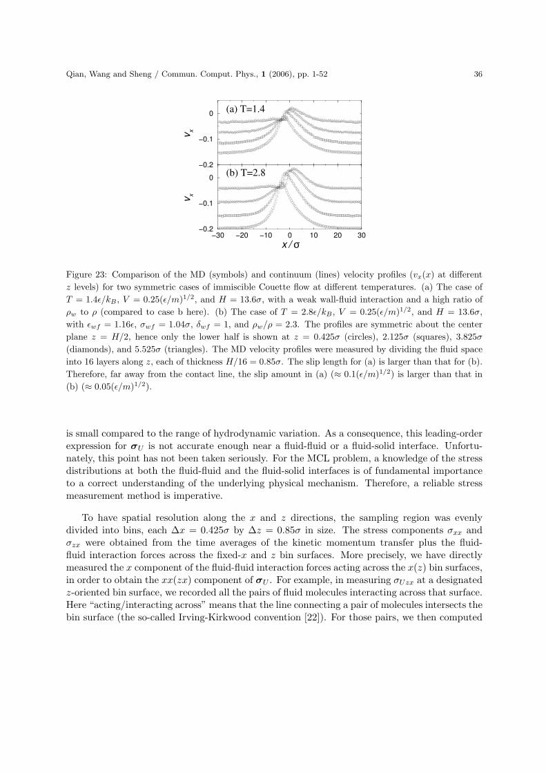
Qian, Wang and Sheng / Commun. Comput. Phys., 1 (2006), pp. 1-52 36
−30 −20 −10 0 10 20 30
x /
−0.2
−0.1
0
vx
−0.2
−0.1
0
vx
σ
(a) T=1.4
(b) T=2.8
Figure 23: Comparison of the MD (symbols) and continuum (lines) velocity profiles (vx(x) at different
z levels) for two symmetric cases of immiscible Couette flow at different temperatures. (a) The case of
T = 1.4ε/kB , V = 0.25(ε/m)1/2, and H = 13.6σ, with a weak wall-fluid interaction and a high ratio of
ρw to ρ (compared to case b here). (b) The case of T = 2.8ε/kB , V = 0.25(ε/m)1/2, and H = 13.6σ,
with εwf = 1.16ε, σwf = 1.04σ, δwf = 1, and ρw/ρ = 2.3. The profiles are symmetric about the center
plane z = H/2, hence only the lower half is shown at z = 0.425σ (circles), 2.125σ (squares), 3.825σ
(diamonds), and 5.525σ (triangles). The MD velocity profiles were measured by dividing the fluid space
into 16 layers along z, each of thickness H/16 = 0.85σ. The slip length for (a) is larger than that for (b).
Therefore, far away from the contact line, the slip amount in (a) (≈ 0.1(ε/m)1/2) is larger than that in
(b) (≈ 0.05(ε/m)1/2).
is small compared to the range of hydrodynamic variation. As a consequence, this leading-orderexpression for σU is not accurate enough near a fluid-fluid or a fluid-solid interface. Unfortu-nately, this point has not been taken seriously. For the MCL problem, a knowledge of the stressdistributions at both the fluid-fluid and the fluid-solid interfaces is of fundamental importanceto a correct understanding of the underlying physical mechanism. Therefore, a reliable stressmeasurement method is imperative.
To have spatial resolution along the x and z directions, the sampling region was evenlydivided into bins, each ∆x = 0.425σ by ∆z = 0.85σ in size. The stress components σxx andσzx were obtained from the time averages of the kinetic momentum transfer plus the fluid-fluid interaction forces across the fixed-x and z bin surfaces. More precisely, we have directlymeasured the x component of the fluid-fluid interaction forces acting across the x(z) bin surfaces,in order to obtain the xx(zx) component of σU . For example, in measuring σUzx at a designatedz-oriented bin surface, we recorded all the pairs of fluid molecules interacting across that surface.Here “acting/interacting across” means that the line connecting a pair of molecules intersects thebin surface (the so-called Irving-Kirkwood convention [22]). For those pairs, we then computed
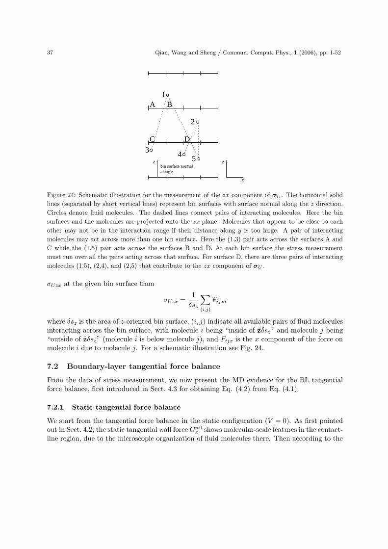
37 Qian, Wang and Sheng / Commun. Comput. Phys., 1 (2006), pp. 1-52
z
x
A
D
1
2
3 4 5
C
B
z
along zbin surface normal
Figure 24: Schematic illustration for the measurement of the zx component of σU . The horizontal solid
lines (separated by short vertical lines) represent bin surfaces with surface normal along the z direction.
Circles denote fluid molecules. The dashed lines connect pairs of interacting molecules. Here the bin
surfaces and the molecules are projected onto the xz plane. Molecules that appear to be close to each
other may not be in the interaction range if their distance along y is too large. A pair of interacting
molecules may act across more than one bin surface. Here the (1,3) pair acts across the surfaces A and
C while the (1,5) pair acts across the surfaces B and D. At each bin surface the stress measurement
must run over all the pairs acting across that surface. For surface D, there are three pairs of interacting
molecules (1,5), (2,4), and (2,5) that contribute to the zx component of σU .
σUzx at the given bin surface from
σUzx =1
δsz
∑
(i,j)
Fijx,
where δsz is the area of z-oriented bin surface, (i, j) indicate all available pairs of fluid moleculesinteracting across the bin surface, with molecule i being “inside of zδsz” and molecule j being“outside of zδsz” (molecule i is below molecule j), and Fijx is the x component of the force onmolecule i due to molecule j. For a schematic illustration see Fig. 24.
7.2 Boundary-layer tangential force balance
From the data of stress measurement, we now present the MD evidence for the BL tangentialforce balance, first introduced in Sect. 4.3 for obtaining Eq. (4.2) from Eq. (4.1).
7.2.1 Static tangential force balance
We start from the tangential force balance in the static configuration (V = 0). As first pointedout in Sect. 4.2, the static tangential wall force Gw0
x shows molecular-scale features in the contact-line region, due to the microscopic organization of fluid molecules there. Then according to the
Qian, Wang and Sheng / Commun. Comput. Phys., 1 (2006), pp. 1-52 38
local force balance, static fluid stress must vary in such a way that the total force density vanishes.An integrated form of the static tangential force balance is given by Gw0
x (x)+Gf0x (x) = 0, where
Gw0x (x) =
∫ z0
0 dzgw0x (x, z) and the static tangential fluid force Gf0
x (x) is of the form
Gf0x (x) =
∫ z0
0dz[∂xσ0
xx(x, z) + ∂zσ0zx(x, z)] = σ0
zx(x, z0) + ∂x
∫ z0
0dzσ0
xx(x, z). (7.1)
Here σ0xx and σ0
zx are the xx and zx components of fluid stress in the static configuration, bothmeasured as reference quantities. In Fig. 25 we show
∫ z0
0 dzσ0xx, σ0
zx(z0), Gf0x , and Gw0
x (whichis the same as in Fig. 14b). In the symmetric case,
∫
int dxσ0zx(x, z0)
∫
int dx∂x
∫ z0
0 dzσ0xx(x, z),
and∫
int dx∫ z0
0 dzgw0x (x, z) all vanish because θsurf
s = 90◦. For the asymmetric case, Gw0x (x) +
Gf0x (x) = 0 means
σ0zx(x, z0) + ∂x
∫ z0
0dzσ0
xx(x, z) +
∫ z0
0dzgw0
x (x, z) = 0, (7.2)
which corresponds to the continuum equation (Eq. (5.3))[
σYzx + ∂xγwf
]
φeq
= 0 at the solid
surface. Here σ0zx(x, z0) corresponds to the continuum σY
zx(φeq) at the solid surface while∂x
∫ z0
0 dzσ0xx +
∫ z0
0 dzgw0x corresponds to the continuum ∂xγwf (φeq) at the solid surface. The
Young’s equation (Eq. (3.7)) γ cos θsurfs +∆γwf = 0 is then obtained through integration, using
∫
intdxσ0
zx(x, z0) =
∫
intdxσY
zx = γ cos θsurfs (7.3)
and∫
intdx∂x
∫ z0
0dzσ0
xx +
∫
intdx
∫ z0
0dzgw0
x =
∫
intdx∂xγwf = ∆γwf . (7.4)
Here γ cos θsurfs and ∆γwf are the two tangential forces per unit length along the contact line
(along y), the former due to the tilt of the fluid-fluid interface (θsurfs 6= 90◦) while the latter due
to the different wall-fluid interactions for the two fluid species. In fact, equations (7.3) and (7.4)
are the microscopic definitions for the two continuum quantities γ cos θsurfs and ∆γwf in the
Young’s equation, whose validity is based on the microscopic tangential force balance expressedin Eq. (7.2).
7.2.2 Dynamic tangential force balance
An integrated form of the dynamic tangential force balance is given by Gwx (x) + Gf
x(x) = 0,
where Gwx (x) =
∫ z0
0 dzgwx (x, z) and the dynamic tangential fluid force Gf
x(x) is of the form
Gfx(x) =
∫ z0
0dz[∂xσxx(x, z) + ∂zσzx(x, z)] = σzx(x, z0) + ∂x
∫ z0
0dzσxx(x, z). (7.5)
Here σxx and σzx are the xx and zx components of fluid stress in the dynamic configuration. InFig. 26 we show
∫ z0
0 dzσxx, σzx(z0), and Gwx . From a comparison between Figs. 25 and 26, we
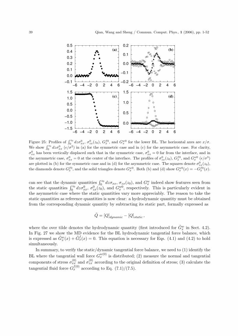
39 Qian, Wang and Sheng / Commun. Comput. Phys., 1 (2006), pp. 1-52
−6 −4 −2 0 2 4 6−1.5
−1.0
−0.5
0.0
0.5
1.0
1.5
−6 −4 −2 0 2 4 6−0.1
0.0
0.1
0.2
0.3
0.4
0.5
−6 −4 −2 0 2 4 6
0.0
0.5
1.0
1.5
−6 −4 −2 0 2 4 6−0.2
−0.1
0.0
0.1
0.2(a)
(c)
(b)
(d)
Figure 25: Profiles of∫ z0
0dzσ0
xx, σ0zx(z0), Gf0
x , and Gw0x for the lower BL. The horizontal axes are x/σ.
We show∫ z0
0dzσ0
xx (ε/σ2) in (a) for the symmetric case and in (c) for the asymmetric case. For clarity,
σ0xx has been vertically displaced such that in the symmetric case, σ0
xx = 0 far from the interface, and in
the asymmetric case, σ0xx = 0 at the center of the interface. The profiles of σ0
zx(z0), Gf0x , and Gw0
x (ε/σ3)
are plotted in (b) for the symmetric case and in (d) for the asymmetric case. The squares denote σ0zx(z0),
the diamonds denote Gf0x , and the solid triangles denote Gw0
x . Both (b) and (d) show Gw0x (x) = −Gf0
x (x).
can see that the dynamic quantities∫ z0
0 dzσxx, σzx(z0), and Gwx indeed show features seen from
the static quantities∫ z0
0 dzσ0xx, σ0
zx(z0), and Gw0x , respectively. This is particularly evident in
the asymmetric case where the static quantities vary more appreciably. The reason to take thestatic quantities as reference quantities is now clear: a hydrodynamic quantity must be obtainedfrom the corresponding dynamic quantity by subtracting its static part, formally expressed as
Q = [Q]dynamic − [Q]static ,
where the over tilde denotes the hydrodynamic quantity (first introduced for Gwx in Sect. 4.2).
In Fig. 27 we show the MD evidence for the BL hydrodynamic tangential force balance, whichis expressed as Gw
x (x) + Gfx(x) = 0. This equation is necessary for Eqs. (4.1) and (4.2) to hold
simultaneously.
In summary, to verify the static/dynamic tangential force balance, we need to (1) identify the
BL where the tangential wall force Gw(0)x is distributed; (2) measure the normal and tangential
components of stress σ(0)xx and σ
(0)zx according to the original definition of stress; (3) calculate the
tangential fluid force Gf(0)x according to Eq. (7.1)/(7.5).

Qian, Wang and Sheng / Commun. Comput. Phys., 1 (2006), pp. 1-52 40
−20 −10 0 10 20−11
−10
−9
−8
−7
−20 −10 0 10 20−11.0
−10.5
−10.0
−9.5
−20 −10 0 10 20
0.0
0.6
1.2
1.8
−20 −10 0 10 20
−0.2
0.0
0.2
0.4
0.6
0.8
(a)
(c)
(b)
(d)
Figure 26: Profiles of∫ z0
0dzσxx, σzx(z0), and Gw
x for the lower BL. The horizontal axes are x/σ. We
show∫ z0
0dzσxx (ε/σ2) in (a) for the symmetric case (V = 0.25
√
ε/m and H = 13.6σ) and in (c) for the
asymmetric case (V = 0.2√
ε/m and H = 13.6σ). The profiles of σzx(z0) and Gwx (ε/σ3) are plotted
in (b) for the symmetric case and in (d) for the asymmetric case. The squares denote σzx(z0) and the
diamonds denote Gwx . Note that in the vicinity of the contact line, Gw
x + σzx(z0) 6= 0. The importance of
the x-gradient of the z-integrated normal stress ∂x
∫ z0
0dzσxx is therefore evident.
−20 −10 0 10 20
x /
−0.25
−0.20
−0.15
−0.10
−0.05
0.00
Gx
w a
nd
−G
x
f ~
~
σ
Figure 27: Hydrodynamic force balance for the lower BL. The circles represent the symmetric case (V =
0.25√
ε/m and H = 13.6σ); the squares represent the asymmetric case (V = 0.2√
ε/m and H = 13.6σ).
The empty symbols denote Gwx ; the solid symbols denote −Gf
x. It is seen that Gwx (x) = −Gf
x(x).

41 Qian, Wang and Sheng / Commun. Comput. Phys., 1 (2006), pp. 1-52
7.3 Tangential Young stress
Here we present the MD evidence for the decomposition of the tangential stress. In a dynamicconfiguration, away from the interfacial region the tangential viscous stress σv
zx = η(∂zvx +∂xvz)is the only component in the (single-fluid) tangential stress σzx. But in the (two-fluid) interfacialregion, the tangential stress σzx can be decomposed into a viscous component σv
zx and a non-viscous component σY
zx:
σzx = σvzx + σY
zx, (7.6)
where σvzx is still η(∂zvx + ∂xvz) and σY
zx is the tangential Young stress, satisfying
Σd ≡∫
intdxσY
zx(x, z) = γ cos θd(z). (7.7)
Here θd(z) is the dynamic interfacial angle at level z. Equation (7.6) is essential to obtainingEq. (5.4) for σzx(x, 0). In a static configuration, the viscous stress σv
zx vanishes and σzx becomesσ0
zx, satisfying
Σs ≡∫
intdxσ0
zx(x, z) = γ cos θs(z), (7.8)
where θs(z) is the static interfacial angle at level z. Fig. 28 shows that both σYzx and σ0
zx arenonzero in the interfacial region only. The inset to Fig. 28 shows the evidence for Eqs. (7.7)and (7.8), which identify σY
zx and σ0zx as the dynamic and static Young stresses.
Equations (7.7) and (7.8) can be derived from the mechanical definition for the interfacialtension γ [26]:
γ =
∫
intdlm
[
P⊥(lm) − P‖(lm)]
,
i.e., γ is the integral (along the interface normal across the interface) of the difference between thenormal and parallel components of the pressure, where lm is the coordinate along the interfacenormal m, and P⊥ and P‖ are the pressure-tensor components normal and parallel to theinterface, respectively. (Note that far away from the interface the pressure is isotropic andP⊥ = P‖). When the interfacial angle θd (or θs) is 90◦, the interface normal m = x and thenon-viscous stress tensor in the interfacial region is diagonal in the xyz coordinate system:
σnon−viscous =
−P⊥ 0 00 −P‖ 0
0 0 −P‖
= −P⊥I + (P⊥ − P‖)(I − mm),
where I is the identity matrix. According to this expression, when the interfacial angle θd (or θs)deviates from 90◦ (see Fig. 29), the Young stress σY
zx (or σ0zx) arises from the interfacial stress
anisotropy as the off-diagonal zx component of the microscopic stress tensor:
σY (0)zx = z · σnon−viscous · x = (P⊥ − P‖) [z · (I − mm) · x]
= −(P⊥ − P‖)mzmx = (P⊥ − P‖) cos θd(s) sin θd(s),
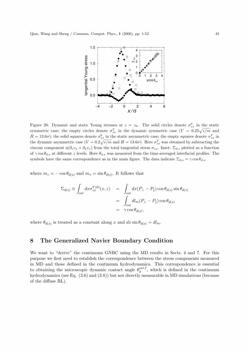
Qian, Wang and Sheng / Commun. Comput. Phys., 1 (2006), pp. 1-52 42
−4 −2 0 2 4 6
x /
0.0
0.5
1.0
1.5
tangential Y
oung s
tress
0 1 2 3 4
γ θ
0
1
2
3
4
Σ
σ
cos d,s
d,s
Figure 28: Dynamic and static Young stresses at z = z0. The solid circles denote σ0zx in the static
symmetric case; the empty circles denote σYzx in the dynamic symmetric case (V = 0.25
√
ε/m and
H = 13.6σ); the solid squares denote σ0zx in the static asymmetric case; the empty squares denote σY
zx in
the dynamic asymmetric case (V = 0.2√
ε/m and H = 13.6σ). Here σYzx was obtained by subtracting the
viscous component η(∂zvx + ∂xvz) from the total tangential stress σzx. Inset: Σd,s plotted as a function
of γ cos θd,s at different z levels. Here θd,s was measured from the time-averaged interfacial profiles. The
symbols have the same correspondence as in the main figure. The data indicate Σd,s = γ cos θd,s.
where mz = − cos θd(s) and mx = sin θd(s). It follows that
Σd(s) ≡∫
intdxσY (0)
zx (x, z) =
∫
intdx(P⊥ − P‖) cos θd(s) sin θd(s)
=
∫
intdlm(P⊥ − P‖) cos θd(s)
= γ cos θd(s),
where θd(s) is treated as a constant along x and dx sin θd(s) = dlm.
8 The Generalized Navier Boundary Condition
We want to “derive” the continuum GNBC using the MD results in Sects. 4 and 7. For thispurpose we first need to establish the correspondence between the stress components measuredin MD and those defined in the continuum hydrodynamics. This correspondence is essentialto obtaining the microscopic dynamic contact angle θsurf
d , which is defined in the continuumhydrodynamics (see Eq. (3.6) and (3.8)) but not directly measurable in MD simulations (becauseof the diffuse BL).

43 Qian, Wang and Sheng / Commun. Comput. Phys., 1 (2006), pp. 1-52
z
x
dl
dx
m d(s)θm
fluid−fluid interface
Figure 29: Schematic illustration for the origin of the tangential Young stress σY (0)zx as an off-diagonal
component of the microscopic stress tensor.
8.1 MD-continuum correspondence
It has been verified that for a BL of finite thickness, the GNBC is given by
βvslipx (x) = Gf
x(x) − Gf0x (x)
=∂
∂x
∫ z0
0dz
[
σxx(x, z) − σ0xx(x, z)
]
+[
σzx(x, z0) − σ0zx(x, z0)
]
,(8.1)
in which only MD measurable quantities are involved. Now we interpret these MD-measuredquantities in terms of the various continuum variables in the hydrodynamic model. In so doingit is essential to note the following. (1) σxx can be decomposed into a molecular componentand a hydrodynamic component: σxx = Txx + σHD
xx . Meanwhile, σ0xx can be composed into
the same molecular component and a hydrostatic component: σ0xx = Txx + σHS
xx . Physically,Txx is the normal stress σ0
xx for the case of a flat, static fluid-fluid interface. Such an interfaceexists in the symmetric case (θsurf
s = 90◦) for any value of H. It also exists in the asym-
metric case (θsurfs 6= 90◦) for H → ∞ (with vanishing curvature ∼ 1/H). In either case, the
interface has zero curvature and the hydrostatic stress σHSxx vanishes according to the Laplace’s
equation: σ0xx → Txx as σHS
xx → 0. (To be more precise, γ cos θsurfs and ∆γwf should be de-
fined in Eqs. (7.3) and (7.4) when the fluid-fluid interface has zero curvature. However, in the
asymmetric case where ∆γwf (= −γ cos θsurfs ) is nonzero, there is a static interfacial curvature
≈ 2 cos θsurfs /H. This results in a hydrostatic σHS
xx , which should be subtracted from σ0xx in the
left-hand side of Eq. (7.4). That is, ∆γwf should be obtained with σ0xx replaced by Txx. Mean-
while, due to the static interfacial curvature, the static interfacial angle θs(z0) determined by
cos θs(z0) = γ−1∫
int dxσ0zx(x, z0) is a bit different from the true θsurf
s . In fact, cos θs(z0) deviates
from cos θsurfs by the BL-integrated curvature ≈ 2z0 cos θsurf
s /H.) The molecular componentTxx exists even if there is no hydrodynamic fluid motion or fluid-fluid interfacial curvature. Onthe contrary, the hydrodynamic component σHD
xx arises from the hydrodynamic fluid motionand interfacial curvature. In the static configuration, σHD
xx becomes σHSxx , which comes from the
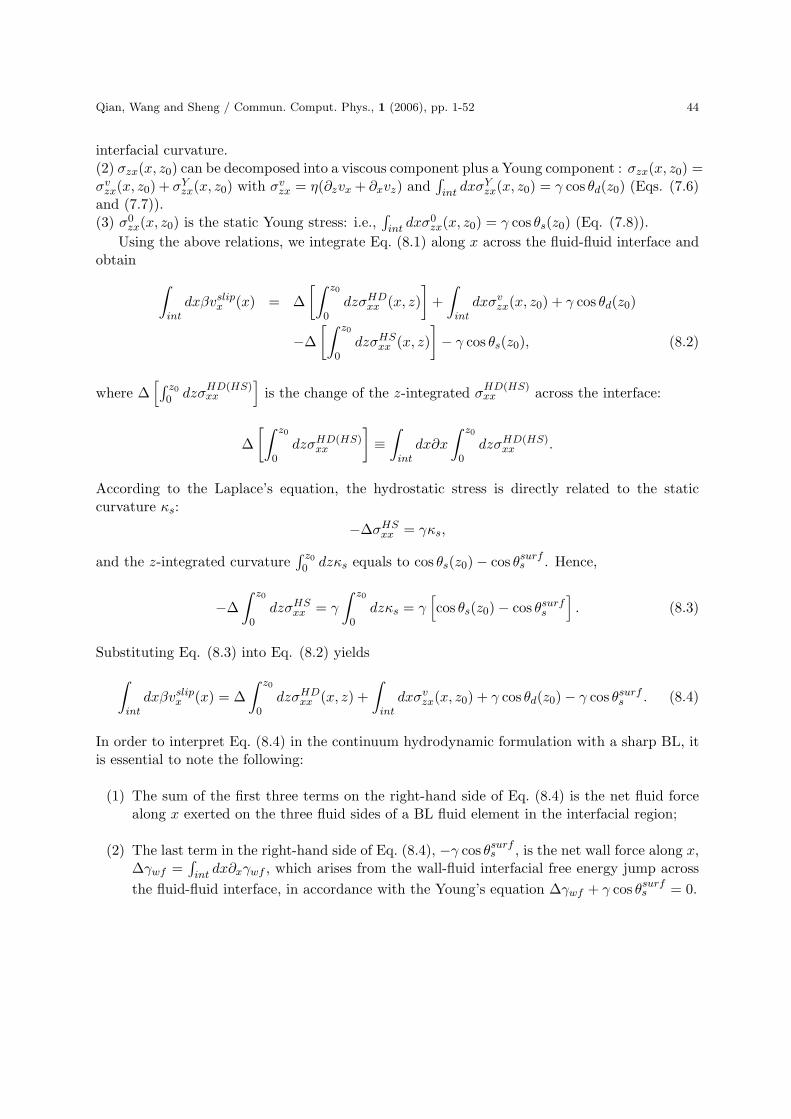
Qian, Wang and Sheng / Commun. Comput. Phys., 1 (2006), pp. 1-52 44
interfacial curvature.(2) σzx(x, z0) can be decomposed into a viscous component plus a Young component : σzx(x, z0) =σv
zx(x, z0) + σYzx(x, z0) with σv
zx = η(∂zvx + ∂xvz) and∫
int dxσYzx(x, z0) = γ cos θd(z0) (Eqs. (7.6)
and (7.7)).(3) σ0
zx(x, z0) is the static Young stress: i.e.,∫
int dxσ0zx(x, z0) = γ cos θs(z0) (Eq. (7.8)).
Using the above relations, we integrate Eq. (8.1) along x across the fluid-fluid interface andobtain
∫
intdxβvslip
x (x) = ∆
[∫ z0
0dzσHD
xx (x, z)
]
+
∫
intdxσv
zx(x, z0) + γ cos θd(z0)
−∆
[∫ z0
0dzσHS
xx (x, z)
]
− γ cos θs(z0), (8.2)
where ∆[
∫ z0
0 dzσHD(HS)xx
]
is the change of the z-integrated σHD(HS)xx across the interface:
∆
[∫ z0
0dzσHD(HS)
xx
]
≡∫
intdx∂x
∫ z0
0dzσHD(HS)
xx .
According to the Laplace’s equation, the hydrostatic stress is directly related to the staticcurvature κs:
−∆σHSxx = γκs,
and the z-integrated curvature∫ z0
0 dzκs equals to cos θs(z0) − cos θsurfs . Hence,
−∆
∫ z0
0dzσHS
xx = γ
∫ z0
0dzκs = γ
[
cos θs(z0) − cos θsurfs
]
. (8.3)
Substituting Eq. (8.3) into Eq. (8.2) yields
∫
intdxβvslip
x (x) = ∆
∫ z0
0dzσHD
xx (x, z) +
∫
intdxσv
zx(x, z0) + γ cos θd(z0) − γ cos θsurfs . (8.4)
In order to interpret Eq. (8.4) in the continuum hydrodynamic formulation with a sharp BL, itis essential to note the following:
(1) The sum of the first three terms on the right-hand side of Eq. (8.4) is the net fluid forcealong x exerted on the three fluid sides of a BL fluid element in the interfacial region;
(2) The last term in the right-hand side of Eq. (8.4), −γ cos θsurfs , is the net wall force along x,
∆γwf =∫
int dx∂xγwf , which arises from the wall-fluid interfacial free energy jump across
the fluid-fluid interface, in accordance with the Young’s equation ∆γwf + γ cos θsurfs = 0.
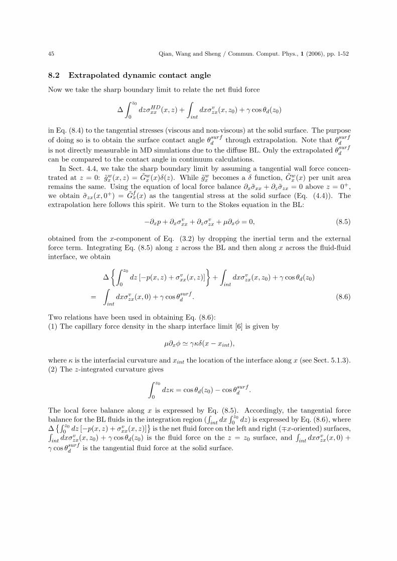
45 Qian, Wang and Sheng / Commun. Comput. Phys., 1 (2006), pp. 1-52
8.2 Extrapolated dynamic contact angle
Now we take the sharp boundary limit to relate the net fluid force
∆
∫ z0
0dzσHD
xx (x, z) +
∫
intdxσv
zx(x, z0) + γ cos θd(z0)
in Eq. (8.4) to the tangential stresses (viscous and non-viscous) at the solid surface. The purpose
of doing so is to obtain the surface contact angle θsurfd through extrapolation. Note that θsurf
d
is not directly measurable in MD simulations due to the diffuse BL. Only the extrapolated θsurfd
can be compared to the contact angle in continuum calculations.
In Sect. 4.4, we take the sharp boundary limit by assuming a tangential wall force concen-trated at z = 0: gw
x (x, z) = Gwx (x)δ(z). While gw
x becomes a δ function, Gwx (x) per unit area
remains the same. Using the equation of local force balance ∂xσxx + ∂zσzx = 0 above z = 0+,we obtain σzx(x, 0+) = Gf
x(x) as the tangential stress at the solid surface (Eq. (4.4)). Theextrapolation here follows this spirit. We turn to the Stokes equation in the BL:
−∂xp + ∂xσvxx + ∂zσ
vzx + µ∂xφ = 0, (8.5)
obtained from the x-component of Eq. (3.2) by dropping the inertial term and the externalforce term. Integrating Eq. (8.5) along z across the BL and then along x across the fluid-fluidinterface, we obtain
∆
{∫ z0
0dz [−p(x, z) + σv
xx(x, z)]
}
+
∫
intdxσv
zx(x, z0) + γ cos θd(z0)
=
∫
intdxσv
zx(x, 0) + γ cos θsurfd . (8.6)
Two relations have been used in obtaining Eq. (8.6):(1) The capillary force density in the sharp interface limit [6] is given by
µ∂xφ ' γκδ(x − xint),
where κ is the interfacial curvature and xint the location of the interface along x (see Sect. 5.1.3).(2) The z-integrated curvature gives
∫ z0
0dzκ = cos θd(z0) − cos θsurf
d .
The local force balance along x is expressed by Eq. (8.5). Accordingly, the tangential forcebalance for the BL fluids in the integration region (
∫
int dx∫ z0
0 dz) is expressed by Eq. (8.6), where∆
{∫ z0
0 dz [−p(x, z) + σvxx(x, z)]
}
is the net fluid force on the left and right (∓x-oriented) surfaces,∫
int dxσvzx(x, z0) + γ cos θd(z0) is the fluid force on the z = z0 surface, and
∫
int dxσvzx(x, 0) +
γ cos θsurfd is the tangential fluid force at the solid surface.
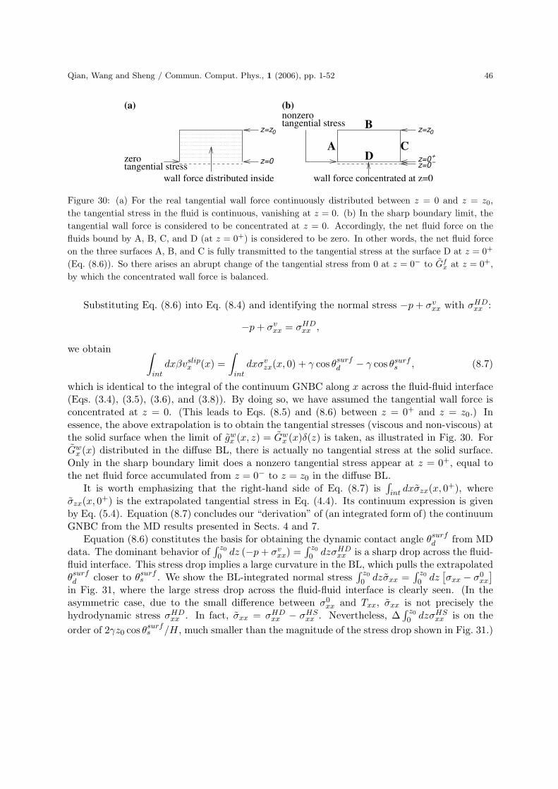
Qian, Wang and Sheng / Commun. Comput. Phys., 1 (2006), pp. 1-52 46
zero
wall force distributed inside
z=0
z=z0
z=0z=0
+−
z=z0
A CD
Btangential stressnonzero
tangential stress
wall force concentrated at z=0
(b)(a)
Figure 30: (a) For the real tangential wall force continuously distributed between z = 0 and z = z0,
the tangential stress in the fluid is continuous, vanishing at z = 0. (b) In the sharp boundary limit, the
tangential wall force is considered to be concentrated at z = 0. Accordingly, the net fluid force on the
fluids bound by A, B, C, and D (at z = 0+) is considered to be zero. In other words, the net fluid force
on the three surfaces A, B, and C is fully transmitted to the tangential stress at the surface D at z = 0+
(Eq. (8.6)). So there arises an abrupt change of the tangential stress from 0 at z = 0− to Gfx at z = 0+,
by which the concentrated wall force is balanced.
Substituting Eq. (8.6) into Eq. (8.4) and identifying the normal stress −p + σvxx with σHD
xx :
−p + σvxx = σHD
xx ,
we obtain∫
intdxβvslip
x (x) =
∫
intdxσv
zx(x, 0) + γ cos θsurfd − γ cos θsurf
s , (8.7)
which is identical to the integral of the continuum GNBC along x across the fluid-fluid interface(Eqs. (3.4), (3.5), (3.6), and (3.8)). By doing so, we have assumed the tangential wall force isconcentrated at z = 0. (This leads to Eqs. (8.5) and (8.6) between z = 0+ and z = z0.) Inessence, the above extrapolation is to obtain the tangential stresses (viscous and non-viscous) atthe solid surface when the limit of gw
x (x, z) = Gwx (x)δ(z) is taken, as illustrated in Fig. 30. For
Gwx (x) distributed in the diffuse BL, there is actually no tangential stress at the solid surface.
Only in the sharp boundary limit does a nonzero tangential stress appear at z = 0+, equal tothe net fluid force accumulated from z = 0− to z = z0 in the diffuse BL.
It is worth emphasizing that the right-hand side of Eq. (8.7) is∫
int dxσzx(x, 0+), whereσzx(x, 0+) is the extrapolated tangential stress in Eq. (4.4). Its continuum expression is givenby Eq. (5.4). Equation (8.7) concludes our “derivation” of (an integrated form of) the continuumGNBC from the MD results presented in Sects. 4 and 7.
Equation (8.6) constitutes the basis for obtaining the dynamic contact angle θsurfd from MD
data. The dominant behavior of∫ z0
0 dz (−p + σvxx) =
∫ z0
0 dzσHDxx is a sharp drop across the fluid-
fluid interface. This stress drop implies a large curvature in the BL, which pulls the extrapolatedθsurfd closer to θsurf
s . We show the BL-integrated normal stress∫ z0
0 dzσxx =∫ z0
0 dz[
σxx − σ0xx
]
in Fig. 31, where the large stress drop across the fluid-fluid interface is clearly seen. (In theasymmetric case, due to the small difference between σ0
xx and Txx, σxx is not precisely thehydrodynamic stress σHD
xx . In fact, σxx = σHDxx − σHS
xx . Nevertheless, ∆∫ z0
0 dzσHSxx is on the
order of 2γz0 cos θsurfs /H, much smaller than the magnitude of the stress drop shown in Fig. 31.)
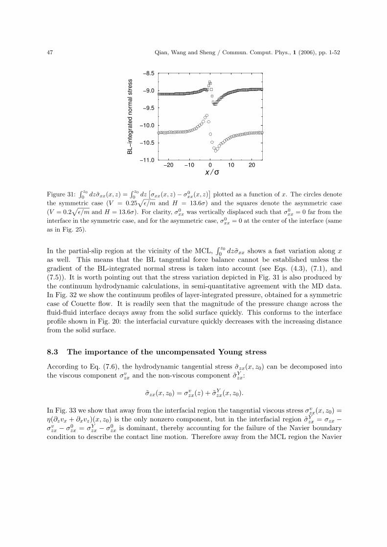
47 Qian, Wang and Sheng / Commun. Comput. Phys., 1 (2006), pp. 1-52
−20 −10 0 10 20
x /
−11.0
−10.5
−10.0
−9.5
−9.0
−8.5
BL−
inte
gra
ted n
orm
al str
ess
σ
Figure 31:∫ z0
0dzσxx(x, z) =
∫ z0
0dz
[
σxx(x, z) − σ0xx(x, z)
]
plotted as a function of x. The circles denote
the symmetric case (V = 0.25√
ε/m and H = 13.6σ) and the squares denote the asymmetric case
(V = 0.2√
ε/m and H = 13.6σ). For clarity, σ0xx was vertically displaced such that σ0
xx = 0 far from the
interface in the symmetric case, and for the asymmetric case, σ0xx = 0 at the center of the interface (same
as in Fig. 25).
In the partial-slip region at the vicinity of the MCL,∫ z0
0 dzσxx shows a fast variation along xas well. This means that the BL tangential force balance cannot be established unless thegradient of the BL-integrated normal stress is taken into account (see Eqs. (4.3), (7.1), and(7.5)). It is worth pointing out that the stress variation depicted in Fig. 31 is also produced bythe continuum hydrodynamic calculations, in semi-quantitative agreement with the MD data.In Fig. 32 we show the continuum profiles of layer-integrated pressure, obtained for a symmetriccase of Couette flow. It is readily seen that the magnitude of the pressure change across thefluid-fluid interface decays away from the solid surface quickly. This conforms to the interfaceprofile shown in Fig. 20: the interfacial curvature quickly decreases with the increasing distancefrom the solid surface.
8.3 The importance of the uncompensated Young stress
According to Eq. (7.6), the hydrodynamic tangential stress σzx(x, z0) can be decomposed intothe viscous component σv
zx and the non-viscous component σYzx:
σzx(x, z0) = σvzx(z) + σY
zx(x, z0).
In Fig. 33 we show that away from the interfacial region the tangential viscous stress σvzx(x, z0) =
η(∂zvx + ∂xvz)(x, z0) is the only nonzero component, but in the interfacial region σYzx = σzx −
σvzx − σ0
zx = σYzx − σ0
zx is dominant, thereby accounting for the failure of the Navier boundarycondition to describe the contact line motion. Therefore away from the MCL region the Navier
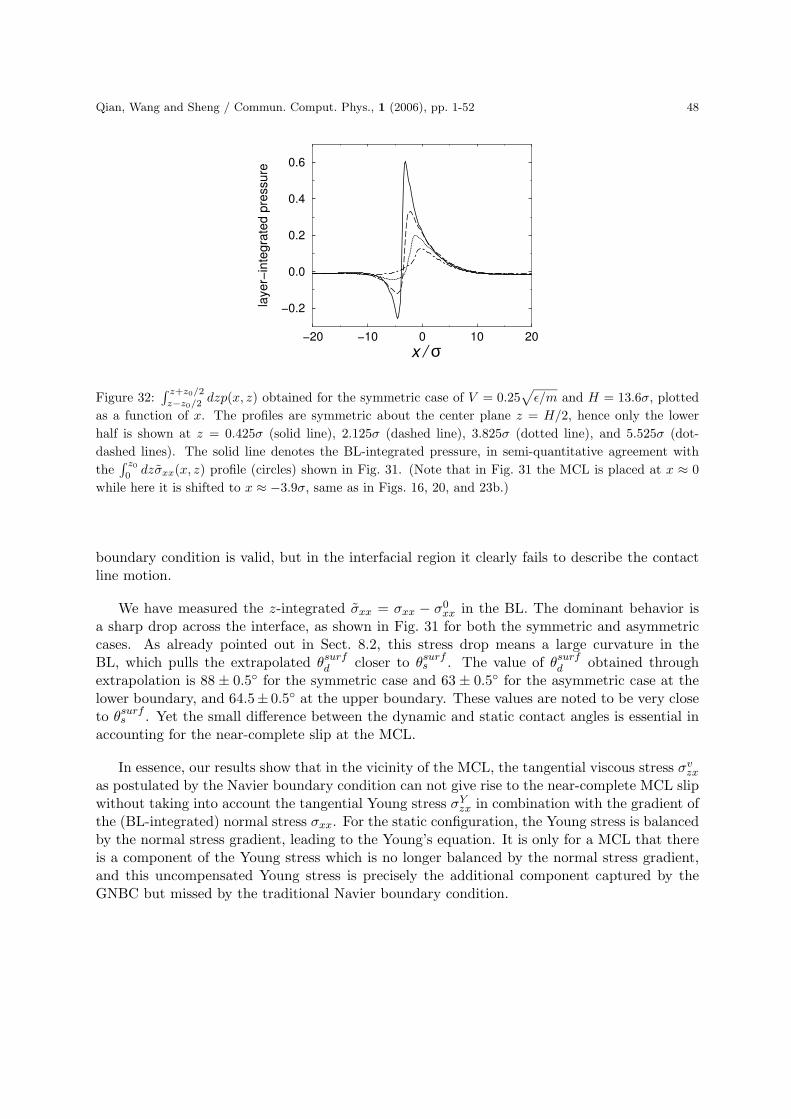
Qian, Wang and Sheng / Commun. Comput. Phys., 1 (2006), pp. 1-52 48
−20 −10 0 10 20
x /
−0.2
0.0
0.2
0.4
0.6
layer−
inte
gra
ted p
ressure
σ
Figure 32:∫ z+z0/2
z−z0/2dzp(x, z) obtained for the symmetric case of V = 0.25
√
ε/m and H = 13.6σ, plotted
as a function of x. The profiles are symmetric about the center plane z = H/2, hence only the lower
half is shown at z = 0.425σ (solid line), 2.125σ (dashed line), 3.825σ (dotted line), and 5.525σ (dot-
dashed lines). The solid line denotes the BL-integrated pressure, in semi-quantitative agreement with
the∫ z0
0dzσxx(x, z) profile (circles) shown in Fig. 31. (Note that in Fig. 31 the MCL is placed at x ≈ 0
while here it is shifted to x ≈ −3.9σ, same as in Figs. 16, 20, and 23b.)
boundary condition is valid, but in the interfacial region it clearly fails to describe the contactline motion.
We have measured the z-integrated σxx = σxx − σ0xx in the BL. The dominant behavior is
a sharp drop across the interface, as shown in Fig. 31 for both the symmetric and asymmetriccases. As already pointed out in Sect. 8.2, this stress drop means a large curvature in theBL, which pulls the extrapolated θsurf
d closer to θsurfs . The value of θsurf
d obtained throughextrapolation is 88 ± 0.5◦ for the symmetric case and 63 ± 0.5◦ for the asymmetric case at thelower boundary, and 64.5± 0.5◦ at the upper boundary. These values are noted to be very closeto θsurf
s . Yet the small difference between the dynamic and static contact angles is essential inaccounting for the near-complete slip at the MCL.
In essence, our results show that in the vicinity of the MCL, the tangential viscous stress σvzx
as postulated by the Navier boundary condition can not give rise to the near-complete MCL slipwithout taking into account the tangential Young stress σY
zx in combination with the gradient ofthe (BL-integrated) normal stress σxx. For the static configuration, the Young stress is balancedby the normal stress gradient, leading to the Young’s equation. It is only for a MCL that thereis a component of the Young stress which is no longer balanced by the normal stress gradient,and this uncompensated Young stress is precisely the additional component captured by theGNBC but missed by the traditional Navier boundary condition.

49 Qian, Wang and Sheng / Commun. Comput. Phys., 1 (2006), pp. 1-52
−10 −5 0 5 10 15
x /
0.0
0.2
0.4
0.6
tan
ge
ntia
l str
ess
σ
(εσ−3
)
Figure 33: Two components of the hydrodynamic tangential stress at z = z0, plotted as a function
of x. The symbols connected by dashed lines denote σYzx; the solid and dotted lines represent the
viscous component. Here the symmetric case is represented by circles and solid line; the asymmetric case
represented by squares and dotted line. In the contact line region the non-viscous component is almost
one order of magnitude larger than the viscous component. The difference between the two components,
however, diminishes towards the boundary, z = 0, due to the large interfacial pressure drop (implying a
large curvature) in the BL, thereby pulling θsurfd closer to θsurf
s .
9 Concluding remarks
In summary, we have found the slip boundary condition, i.e., the GNBC, for the contact-linemotion. Based on this finding, we have formulated a hydrodynamic model that is capable ofreproducing the MD results of slip profile, including the near-complete slip at the MCL. It shouldbe noted, however, that the present continuum formulation can not calculate fluctuation effectsthat are important in MD simulations.
Based on the results and experiences obtained in the present study of the MCL, we havebeen working on the following.
(1) Large scale MD simulations on two-phase immiscible flows show that associated with theMCL, there is a very large 1/x partial-slip region, where x denotes the distance from the contactline. This power-law partial-slip region has been reproduced in large-scale adaptive continuumcalculations [35, 37] based on the local, continuum hydrodynamic formulation presented in thispaper. MD simulations and continuum solutions both indicate the existence of a universal slipprofile in the Stokes-flow regime, well described by vslip(x)/V = 1/(1 + x/als), where vslip isthe slip velocity, V the speed of moving wall, ls the slip length, and a is a numerical constant∼ 1 [35]. A large 1/x partial slip region is significant, because the outer cutoff length scaledirectly determines the integrated effects, such as the total steady-state dissipation. While inthe past the 1/x stress variation away from the MCL has been known [20], to our knowledgethe fact that the partial slip also exhibits the same spatial dependence has not been previously
Qian, Wang and Sheng / Commun. Comput. Phys., 1 (2006), pp. 1-52 50
seen, even though the validity of the Navier boundary condition at high shear stress has beenverified [2, 8, 39,41].
(2) By explicitly taking into account the long-range wall-fluid interactions, our hydrodynamicmodel for two-phase immiscible flow at the solid surface can be used to investigate the dryspreading of a pure, nonvolatile liquid, attracted towards the solid by long-range van der Waalsforces [12]. The precursor film, driven by the gradient of disjoining pressure due to the long-rangeforce [9], was observed decades ago [13, 17, 25]. Nevertheless, the theoretical analysis remainsto be difficult, because of a wide separation of different length scales involved [12, 14, 18, 32].Application of our model to this multi-scale problem is currently underway.
(3) Decades ago it became well known that the driven cavity flow is incompatible with the no-slip boundary condition, since the latter would lead to stress singularity and infinite dissipation(known as corner-flow singularity) [3, 29]. While MD studies [27] have clearly demonstratedrelative fluid-wall slipping near the corner intersection, the exact rule that governs this relativeslip has been left unresolved. Based on the simulation technique developed in the present study,we have verified the validity of the Navier boundary condition in governing the fluid slippingin driven cavity flows. We have used this discovery to formulate a continuum hydrodynamicswhose predictions are in remarkable quantitative agreement with the MD simulation results atthe molecular level [33].
Acknowledgments
The authors would like to thank Weinan E and Weiqing Ren for helpful discussions. This workwas partially supported by the grants DAG03/04.SC21 and RGC-CERG 604803.
References
[1] M. Allen and D. Tildesley, Computer Simulation of Liquids, Clarendon, New York, 1987.[2] J-L. Barrat and L. Bocquet, Large slip effect at a nonwetting fluid-solid interface, Phys. Rev. Lett.,
82 (1999), p. 4671; Influence of wetting properties on hydrodynamic boundary conditions at afluid/solid interface, Faraday Discuss., 112 (1999), p. 119.
[3] G.K. Batchelor, An Introduction to Fluid Dynamics, Cambridge University Press, Cambridge, 1991.[4] T. D. Blake and J. M. Haynes, Kinetics of liquid/liquid displacement, J. Colloid Interf. Sci., 30
(1969), p. 421; T. D. Blake, Dynamic contact angles and wetting kinetics, in: J. C. Berg (Ed.),Wettability, Marcel Dekker Inc., 1993, p. 251.
[5] J. W. Cahn and J. E. Hilliard, Free energy of a nonuniform system. I. Interfacial free energy, J.Chem. Phys., 28 (1958), p. 258.
[6] R. Chella and J. Vinals, Mixing of a two-phase fluid by cavity flow, Phys. Rev. E, 53 (1996), p. 3832.[7] H. Y. Chen, D. Jasnow and J. Vinals, Interface and contact line motion in a two phase fluid under
shear flow, Phys. Rev. Lett., 85 (2000), p. 1686.[8] M. Cieplak, J. Koplik and J. R. Banavar, Boundary conditions at a fluid-solid interface, Phys. Rev.
Lett., 86 (2001), p. 803.[9] B. V. Derjaguin, Theory of the capillary condensation and other capillary phenomena taking into
account the disjoining effect of long-chain molecular liquid films (in Russian), Zh. Fiz. Khim., 14(1940), p. 137.
51 Qian, Wang and Sheng / Commun. Comput. Phys., 1 (2006), pp. 1-52
[10] E. B. Dussan V., The moving contact line: the slip boundary condition, J. Fluid Mech., 77 (1976),p. 665.
[11] E. B. Dussan, V., On the spreading of liquids on solid surfaces: static and dynamic contact lines,Ann. Rev. Fluid Mech., 11 (1979), p. 371.
[12] P. G. de Gennes, Wetting: statics and dynamics, Rev. Mod. Phys., 57 (1985), p. 827.[13] H. Ghiradella, W. Radigan and H. L. Frisch, Electrical-resistivity changes in spreading liquid-films,
J. Colloid Interf. Sci., 51 (1975), p. 522.[14] K. B. Glasner, Spreading of droplets under the influence of intermolecular forces, Phys. Fluid, 15
(2003), p. 1837.[15] N. G. Hadjiconstantinou, Combining atomistic and continuum simulations of contact-line motion,
Phys. Rev. E, 59 (1999), p. 2475.[16] N. G. Hadjiconstantinou, Hybrid atomistic-continuum formulations and the moving contact-line
problem, J. Comput. Phys., 154 (1999), p. 245.[17] W. B. Hardy, The spreading of fluids on glass, Philos. Mag., 38 (1919), p. 49.[18] H. Hervet and P. G. de Gennes, Physique des surfaces et des interfaces — Dynamique du mouillage:
films precurseurs sur solide, C. R. Acad. Sci. Paris II, 299 (1984), p. 499.[19] L. M. Hocking, A moving fluid interface. Part 2. The removal of the force singularity by a slip flow,
J. Fluid Mech., 79 (1977), p. 209.[20] C. Hua and L. E. Scriven, Hydrodynamic model of steady movement of a solid/liquid/fluid contact
line, J. Colloid Interf. Sci., 35 (1971), p. 85.[21] C. Huh and S. G. Mason, The steady movement of a liquid meniscus in a capillary tube, J. Fluid
Mech., 81 (1977), p. 401.[22] J. H. Irving and J. G. Kirkwood, The statistical mechanical theory of transport processes. IV. The
equations of hydrodynamics, J. Chem. Phys., 18 (1950), p. 817. For the validity of the Irving-Kirkwood expression, see the paragraph following equation (5.15) in this paper.
[23] J. N. Israelachivili, Intermolecular and Surface Forces (2nd ed), Academic Press, London, 1992.[24] D. Jacqmin, Calculation of two-phase Navier-Stokes flows using phase-field modeling, J. Comput.
Phys. 155 (1999), p. 96; D. Jacqmin, Contact-line dynamics of a diffuse fluid interface, J. Fluid.Mech., 402 (2000), p. 57.
[25] H. P. Kavehpour, B. Ovryn and G. H. McKinley, Microscopic and macroscopic structure of theprecursor layer in spreading viscous drops, Phys. Rev. Lett., 91 (2003), p. 196104.
[26] J. G. Kirkwood and F. P. Buff, The statistical mechanical theory of surface tension, J. Chem. Phys.,17 (1949), p. 338.
[27] J. Koplik and J. R. Banavar, Corner flow in the sliding plate problem, Phys. Fluids, 7 (1995),p. 3118.
[28] J. Koplik, J. R. Banavar and J. F. Willemsen, Molecular dynamics of Poiseuille flow and movingcontact lines, Phys. Rev. Lett., 60 (1988), p. 1282; J. Koplik, J. R. Banavar and J. F. Willemsen,Molecular dynamics of fluid flow at solid surfaces, Phys. Fluids A, 1 (1989), p. 781.
[29] H. K. Moffatt, Viscous and resistive eddies near a sharp corner, J. Fluid. Mech., 18 (1964), p. 1.[30] C. L. M. H. Navier, Memoire sur les lois du mouvement des fluides, Memoires de l’Academie Royale
des Sciences de l’Institut de France, 6 (1823), 389-440.[31] L. M. Pismen and Y. Pomeau, Disjoining potential and spreading of thin liquid layers in the diffuse-
interface model coupled to hydrodynamics, Phys. Rev. E, 62 (2000), p. 2480; L. M. Pismen, Meso-scopic hydrodynamics of contact line motion, Colloid Surface A, 206 (2002), p. 11.
[32] L. M. Pismen, B. Y. Rubinstein and I. Bazhlekov, Spreading of a wetting film under the action ofvan der Waals forces, Phys. Fluid, 12 (2000), p. 480.
[33] T. Z. Qian and X. P. Wang, Driven cavity flow: from molecular dynamics to continuum hydrody-
Qian, Wang and Sheng / Commun. Comput. Phys., 1 (2006), pp. 1-52 52
namics, SIAM Multiscale Model. Simul., 3 (2005), p. 749.[34] T. Z. Qian, X. P. Wang and P. Sheng, Molecular scale contact line hydrodynamics of immiscible
flows, Phys. Rev. E, 68 (2003), p. 016306.[35] T. Z. Qian, X. P. Wang and P. Sheng, Power-law slip profile of the moving contact line in two-phase
immiscible flows, Phys. Rev. Lett., 93 (2004), p. 094501.[36] W. Ren and Weinan E, Heterogeneous multiscale method for the modeling of complex fluids and
micro-fluidics, J. Comput. Phys., 204 (2005), p. 1.[37] W. Ren and X. P. Wang, An iterative grid redistribution method for singular problems in multiple
dimensions, J. Comput. Phys., 159 (2000), p. 246.[38] P. Seppecher, Moving contact lines in the Cahn-Hilliard theory, Int. J. Engng. Sci., 34 (1996), p. 977.[39] P. A. Thompson and M. O. Robbins, Shear flow near solids: epitaxial order and flow boundary
conditions, Phys. Rev. A, 41 (1990), p. 6830.[40] P. A. Thompson and M. O. Robbins, Simulations of contact-line motion: slip and the dynamic
contact angle, Phys. Rev. Lett., 63 (1989), p. 766; P. A. Thompson, W. B. Brinckerhoff and M. O.Robbins, Microscopic studies of static and dynamic contact angles, J. Adhesion Sci. Tech., 7 (1993),p. 535.
[41] P. A. Thompson and S. M. Troian, A general boundary condition for liquid flow at solid surfaces,Nature, 389 (1997), p. 360.
[42] K. P. Travis and K. E. Gubbins, Poiseuille flow of Lennard-Jones fluids in narrow slit pores, J.Chem. Phys., 112 (2000), p. 1984.
[43] M. Y. Zhou and P. Sheng, Dynamics of immiscible-fluid displacement in a capillary tube, Phys.Rev. Lett., 64 (1990), p. 882; P. Sheng and M. Y. Zhou, Immiscible-fluid displacement: Contact-linedynamics and the velocity-dependent capillary pressure, Phys. Rev. A, 45 (1992), p. 5694.