Momentum and Energy Transfer betweenCoupled Mass-Spring Chains

Henry Jacobs

June 3, 2009

1 Introduction

In this paper I hope to illustrate how variational integrators can be used in thestudy of momentum and energy transfer, perhaps as a means to understand frictionand dissipation. We will first be looking at a system of two colliding mass-springchains, denoted Ct for the top chain and Cb for the bottom chain. The particlesbetween chains are coupled by a nonlinear potential V2. This creates a repulsiveforce making the model reminiscent of elastic collisions. All the springs are linearwith spring constant k, and all masses are equal with masses mt = mb = 1. Inthe final section will will switch the nonlinear coupling into an attractive force andstudy how Ct transmits the energy to Cb from a random perturbation of a stableequilibrium. This last idea is intended to model heat.

C t

C b

Figure 1: A schematic diagram of the model to be studied. Thegray lines represent the nonlinear coupling betweenthe chains.

1

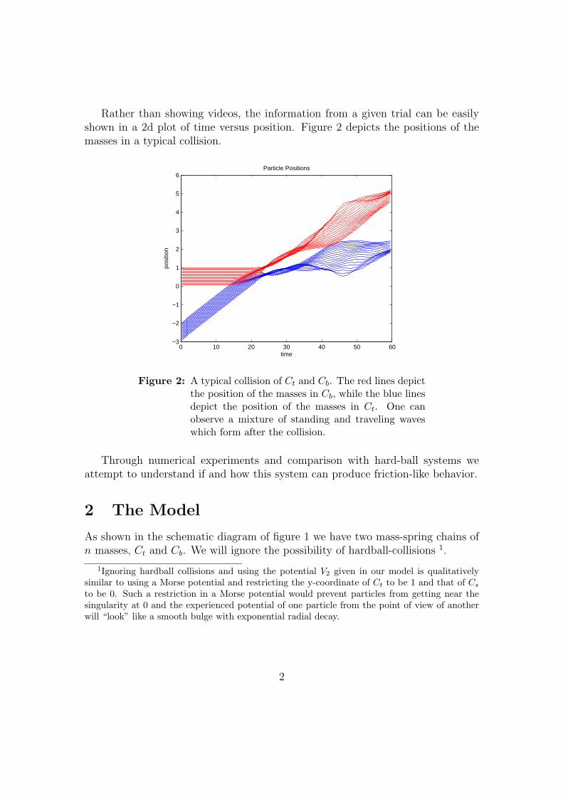
Rather than showing videos, the information from a given trial can be easilyshown in a 2d plot of time versus position. Figure 2 depicts the positions of themasses in a typical collision.

0 10 20 30 40 50 60−3

−2

−1

0

1

2

3

4

5

6Particle Positions

time

posi

tion

Figure 2: A typical collision of Ct and Cb. The red lines depictthe position of the masses in Cb, while the blue linesdepict the position of the masses in Ct. One canobserve a mixture of standing and traveling waveswhich form after the collision.

Through numerical experiments and comparison with hard-ball systems weattempt to understand if and how this system can produce friction-like behavior.

2 The Model

As shown in the schematic diagram of figure 1 we have two mass-spring chains ofn masses, Ct and Cb. We will ignore the possibility of hardball-collisions 1.

1Ignoring hardball collisions and using the potential V2 given in our model is qualitativelysimilar to using a Morse potential and restricting the y-coordinate of Ct to be 1 and that of Cs

to be 0. Such a restriction in a Morse potential would prevent particles from getting near thesingularity at 0 and the experienced potential of one particle from the point of view of anotherwill “look” like a smooth bulge with exponential radial decay.

2

2.1 Equations of Motions

Let qt, qb ∈ Rn store the positions of particles in Ct and Cb respectively. Thepotential energy from the linear springs is given by

V1(qt, qb) =k1

2

n−1∑i=1

(qi+1t − qit − l)2 + (qi+1

b − qib − l)2

Where l is the natural length of the spring, by default we set this to 1N

. By defaultwe set the spring constant k1 = 1.0. The potential energy for the coupling betweenCt and Cb will be

V2(qt, qb) = k2

n∑i,j=1

exp

(−(qit − q

jb)

2

2σ2

)

By defaults we set k2 = 0.001. From observation a higher k prevents a lot ofinteresting interaction for initial velocites less than 1. Together, these potentialfunctions give the total potential energy of V = V1 + V2. The mass of the eachparticle is simply m = 1 and so our kinetic energy can be written

K =m

2‖q̇‖2

We construct the Lagrangian

L(q, q̇) = K(q̇)− V (q)

The Euler-Lagrange equations are the familiar equations of motion for a particlein a potential,

mq̈ +∇V (q) = 0

Explicity these are

mq̈lt + k1(ql+1t − 2qlt + ql−1

t ) + k2

(n∑j=1

1

σ2(qlt − q

jb) exp

(−(qlt − q

jb)

2

2σ2

))= 0

and similarly for qlb

mq̈lb + k1(ql+1b − 2qlb + ql−1

b )− k2

(n∑i=1

1

σ2(qit − qlb) exp

(−(qit − qlb)2

2σ2

))= 0

3

2.2 Conservations of Momentum

As an exercise we show explicitly how to show conservation of linear momentum.It’s easy to see that the continuous system is invariant under the action of the groupG = R of uniform translations in position, simply substitute φr(q

l) = ql(t)+ r intothe Lagrangian (allowing for the abuse of notation that q+ r is the vector qit,b+ r).

L(q + r, q̇) =m

2‖q̇‖2 − V (q + r)

and use that

V1(q + r) =k1

2

n−1∑i=1

((qi+1t + r)− (qit + r)− l)2 + ((qi+1

b + r)− (qib + r)− l)2

=k1

2

n−1∑i=1

(qi+1t − qit − l)2 + (qi+1

b − qib − l)2

= V1(q)

and that

V2(q + r) = k2

n∑i,j=1

exp

(−((qit + r)− (qjb + r))2

2σ2

)

= k2

n∑i,j=1

exp

(−((qit + r)− (qjb + r))2

2σ2

)= V2(q)

We see that the exponential map from the lie-algebra g = R is exp(ξ) = ξ, thusinfinitesimal generator for ξ ∈ g is

ξQ =

ξ...ξ

The corresponding momentum map J : TQ→ g∗ satisfies

〈J(q, q̇), ξ〉 = 〈FL(q, q̇), ξQ〉Where the fiber derivative FL = ∂L

∂q̇in this case. Putting together the pieces we

find

J(q, q̇) = q̇TM ·

1...1

=∑i

mq̇i

We will see later that the analogous arguments for discrete mechanics produce aslightly different discrete momentum.

4

3 Variational Integrators

A variational integrator is formed by maximizing an approximation of the action in-tegral, rather than working with the Euler-Lagrange equations directly. Assumingthe configuration manifold is a vector space, we can approximate the LagrangianL : TQ→ R with Ld : Q×Q→ R defined by

Ld(q1, q2) = L(q1 + q2

2,q2 − q1

∆t)

Where ∆t is some sufficiently small interval of time. We then define the discreteaction integral

Sd[q] =N−1∑k=1

Ld(qk, qk+1)

Which upon setting ∂Sd

∂qk= 0 we find

D1 · Ld(qk, qk+1) +D2 · Ld(qk, qk+1) = 0

A trajectory [q] = {qk}Nk=1 that satisfies the above equation will maximize Sd[q] ,and hence approximately maximize the action integral of the continuous systemover short periods of time (a concern of backward error analysis).

In the case of the typical L = K − V type of Lagrangian the discrete Euler-Lagrange equations are

M

(qk+1 − 2qk + qk−1

h2

)+

1

2

(∇V (

qk+1 + qk2

) +∇V (qk + qk−1

2)

)= 0

This is the method we implement on the Lagrangian explained in section 2 (Seethe Appendix for code).

3.1 Conservation of Discrete Momentum

As an exercise I’ll explicitly show the symmetry that will give conservation of linearmomentum for the system. Let our group be G = R. We define the action on Qto be

Φg(q) = qi + g

That is, we just add g to each coordinate. The action on Q×Q is simply Φ(q0, q1) =(Φ(q0),Φ(q1)). It’s easy to see that this action leaves Ld invariant.

Ld(q1 + r, q2 + r) = L((q1 + r) + (q2 + r)

2,(q2 + r)− (q1 + r)

∆t)

= L(q1 + q2

2+ r,

q2 − q1

∆t)

5

because Φ leave L invariant

= L(q1 + q2

2,q2 − q1

∆t)

= Ld(q1, q2)

The lie algebra is again g = R, and the exponential map is exp(ξ) = ξ ∈ G. Theinfinitesimal generator from Φ is

ξQ×Q =

ξ...ξ

, In the arena of discrete mechanics this symmetry implies a discrete momentummap satisfying

J−Ld(q0, q1) · ξ = 〈Θ−Ld

Ld, ξQ×Q〉(q0, q1)

Where Θ−Ldis the minus discrete Lagrangian one form [1]. In this case

Θ−LdLd =

−1

∆t2(q1 − q0)TM − 1

2dV

(q1 + q0

2

)So that J−Ld

is

J−Ld(q0, q1) =

∑i

1

h2m(qi1 − qi0) +

1

2dV i

(q1 + q0

2

)Not quite what I’d expect. If you caught me off-guard I’d expect the momentumto be Jguess = m

h

∑i (q

i1 − qi0), but this is not quite conserved by the algorithm.

Although Jguess does seem to oscillate quite rapidly with low amplitude (like 10−14)about a constant value, and doesn’t bias towards any one direction. This is likelyrelated to what occures when we take the continuum limit of the discrete momen-tum times the time-step h. If q1 = q(h+ t) and q0 = q(t) we see

limh→0

(h× Jd(q(t+ h), q(t)) =∑i

mq̇i + 0 = J(q, q̇)

4 Numerical Performance

We start in an arrangement where all the particles within each chain are spaced lapart (This is the equilibrium arrangement when V2 is absent). We make a series

6

0 50 100 150 200 250 300 350 400−20

−15

−10

−5

0

5

10

15

20time evolution of positions

time

posi

tion

of p

artic

les

Figure 3: Depicts the position of the particles. Red is for Cband blue is for Ct, it appears I mismatched my labelso that Ct is below Cb.

0 50 100 150 200 250 300 350 4000.049984

0.049986

0.049988

0.04999

0.049992

0.049994

0.049996

0.049998

0.05

0.050002

time

Ene

rgy

Figure 4: Energy Preservation properties, Note the scale on they-axis. The largest change in total energy is 3.3944×10−04 of the largest change in potential energy.

7

of observations on the quality of the integrator for Ct and Cb initially separatedby a distance of 3, heading towards each other with an initial velocity v0 = 0.1and. The evolution of the particles is depicted in figure 3

We observe that the algorithm does a very good job of preserving energy andsymmetries. Figure 4 depicts how energy evolves in time.

to find φ∗L = L. This gives us conservation of linear momentum via Noether’stheorem. This is shown to hold for a general system of N particles on the config-uration manifold Q = R3N in [1], section 11.4. The momentum map is found tobe J(ξr)(q, p) =

∑p. In the discrete case we notice that Ld is invariant under the

same symmetry since Thus Ld is invariant as well and we can apply the discreteNoether’s theorem as described in [2]. We get a discrete momentum map∑

i

1

h2m(qi1 − qi0) +

1

2dV i

(q1 + q0

2

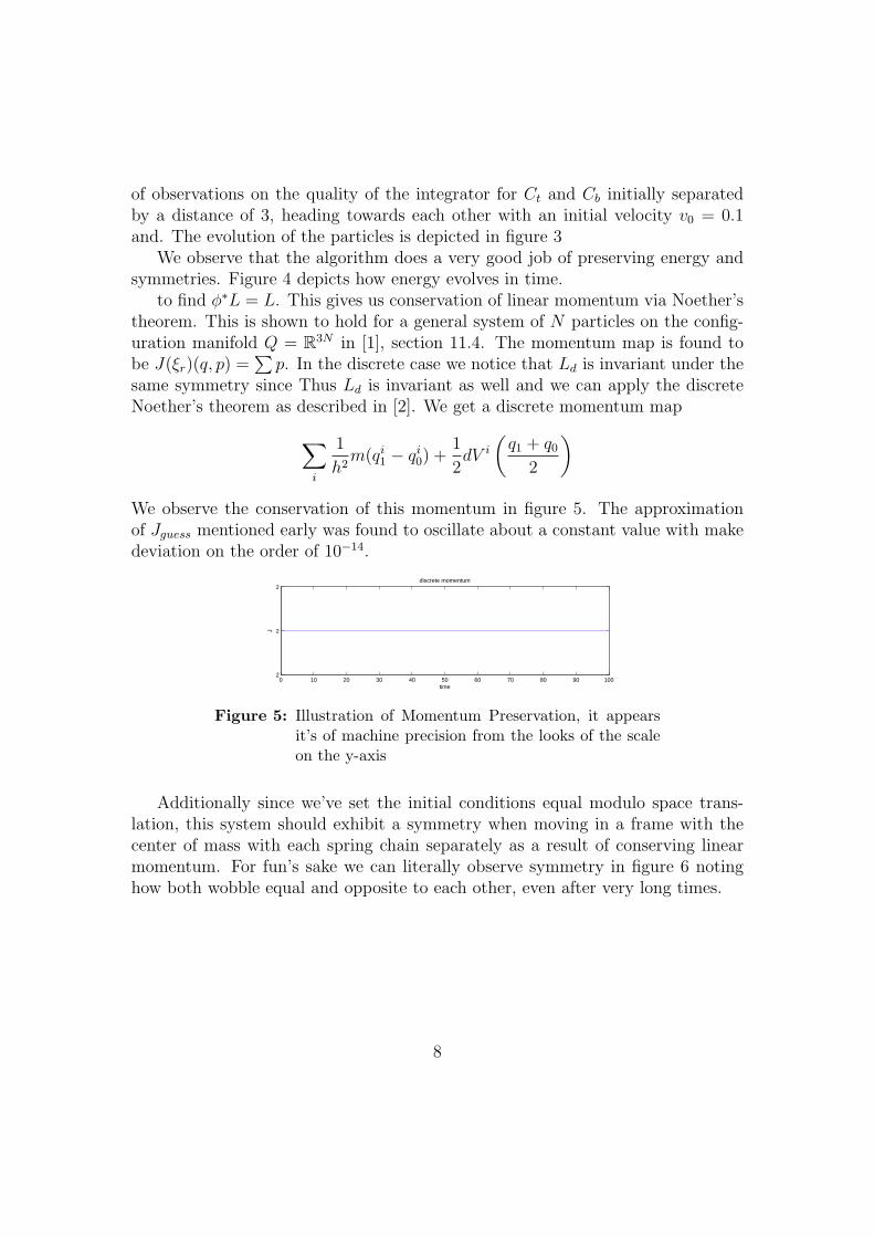
)We observe the conservation of this momentum in figure 5. The approximationof Jguess mentioned early was found to oscillate about a constant value with makedeviation on the order of 10−14.

0 10 20 30 40 50 60 70 80 90 1002

2

2discrete momentum

time

J

Figure 5: Illustration of Momentum Preservation, it appearsit’s of machine precision from the looks of the scaleon the y-axis

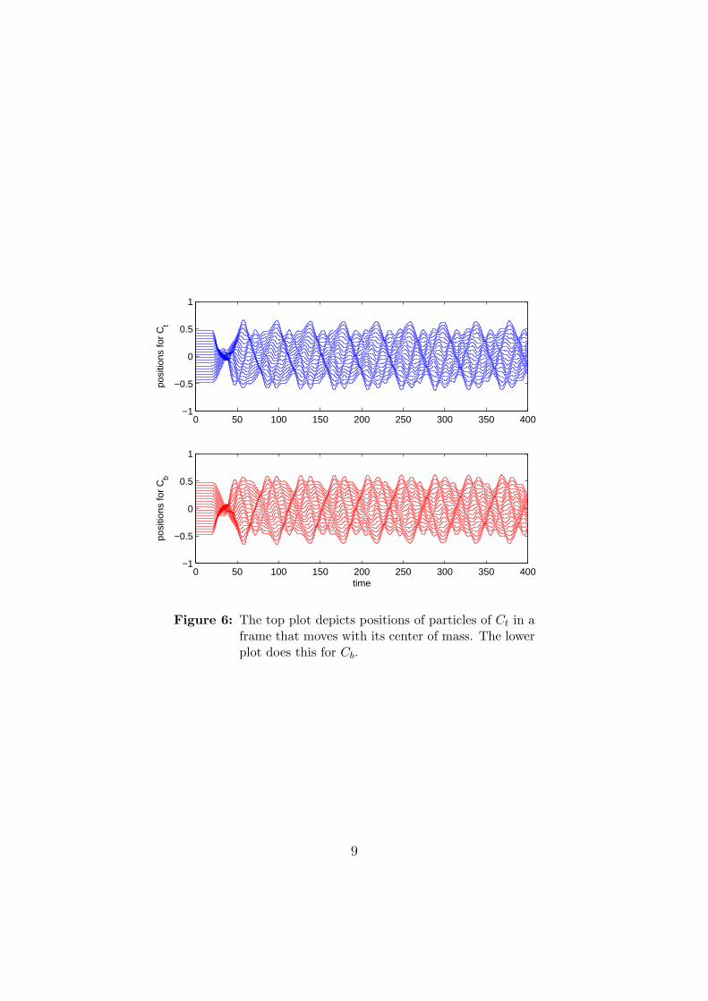
Additionally since we’ve set the initial conditions equal modulo space trans-lation, this system should exhibit a symmetry when moving in a frame with thecenter of mass with each spring chain separately as a result of conserving linearmomentum. For fun’s sake we can literally observe symmetry in figure 6 notinghow both wobble equal and opposite to each other, even after very long times.

8

0 50 100 150 200 250 300 350 400−1

−0.5

0

0.5

1

posi

tions

for

Ct

0 50 100 150 200 250 300 350 400−1

−0.5

0

0.5

1

time

posi

tions

for

Cb

Figure 6: The top plot depicts positions of particles of Ct in aframe that moves with its center of mass. The lowerplot does this for Cb.

9

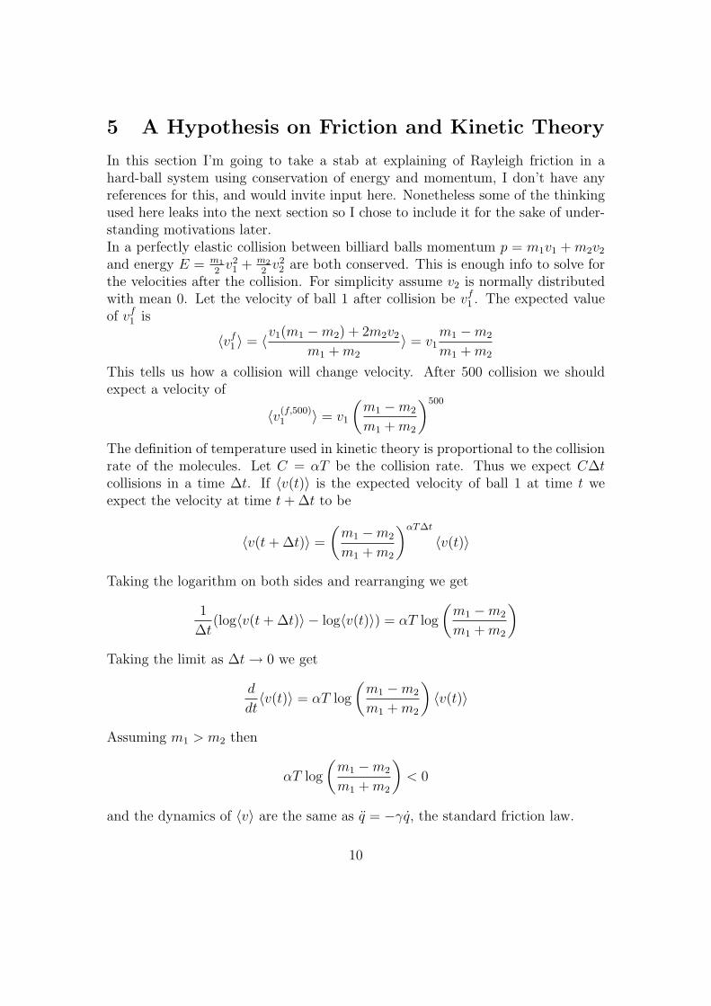
5 A Hypothesis on Friction and Kinetic Theory

In this section I’m going to take a stab at explaining of Rayleigh friction in ahard-ball system using conservation of energy and momentum, I don’t have anyreferences for this, and would invite input here. Nonetheless some of the thinkingused here leaks into the next section so I chose to include it for the sake of under-standing motivations later.In a perfectly elastic collision between billiard balls momentum p = m1v1 + m2v2

and energy E = m1

2v2

1 + m2

2v2

2 are both conserved. This is enough info to solve forthe velocities after the collision. For simplicity assume v2 is normally distributedwith mean 0. Let the velocity of ball 1 after collision be vf1 . The expected valueof vf1 is

〈vf1 〉 = 〈v1(m1 −m2) + 2m2v2

m1 +m2

〉 = v1m1 −m2

m1 +m2

This tells us how a collision will change velocity. After 500 collision we shouldexpect a velocity of

〈v(f,500)1 〉 = v1

(m1 −m2

m1 +m2

)500

The definition of temperature used in kinetic theory is proportional to the collisionrate of the molecules. Let C = αT be the collision rate. Thus we expect C∆tcollisions in a time ∆t. If 〈v(t)〉 is the expected velocity of ball 1 at time t weexpect the velocity at time t+ ∆t to be

〈v(t+ ∆t)〉 =

(m1 −m2

m1 +m2

)αT∆t

〈v(t)〉

Taking the logarithm on both sides and rearranging we get

1

∆t(log〈v(t+ ∆t)〉 − log〈v(t)〉) = αT log

(m1 −m2

m1 +m2

)Taking the limit as ∆t→ 0 we get

d

dt〈v(t)〉 = αT log

(m1 −m2

m1 +m2

)〈v(t)〉

Assuming m1 > m2 then

αT log

(m1 −m2

m1 +m2

)< 0

and the dynamics of 〈v〉 are the same as q̈ = −γq̇, the standard friction law.

10

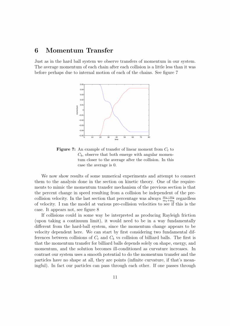
6 Momentum Transfer

Just as in the hard ball system we observe transfers of momentum in our system.The average momentum of each chain after each collision is a little less than it wasbefore perhaps due to internal motion of each of the chains. See figure 7

0 10 20 30 40 50 60 70 80−0.05

−0.04

−0.03

−0.02

−0.01

0

0.01

0.02

0.03

0.04

0.05

time

mom

entu

m

Figure 7: An example of transfer of linear moment from Ct toCb, observe that both emerge with angular momen-tum closer to the average after the collision. In thiscase the average is 0.

We now show results of some numerical experiments and attempt to connectthem to the analysis done in the section on kinetic theory. One of the require-ments to mimic the momentum transfer mechanism of the previous section is thatthe percent change in speed resulting from a collision be independent of the pre-collision velocity. In the last section that percentage was always m1−m2

m1+m2regardless

of velocity. I ran the model at various pre-collision velocities to see if this is thecase. It appears not, see figure 8

If collisions could in some way be interpreted as producing Rayleigh friction(upon taking a continuum limit), it would need to be in a way fundamentallydifferent from the hard-ball system, since the momentum change appears to bevelocity dependent here. We can start by first considering two fundamental dif-ferences between collisions of Ct and Cb vs collision of billiard balls. The first isthat the momentum transfer for billiard balls depends solely on shape, energy, andmomentum, and the solution becomes ill-conditioned as curvature increases. Incontrast our system uses a smooth potential to do the momentum transfer and theparticles have no shape at all, they are points (infinite curvature, if that’s mean-ingful). In fact our particles can pass through each other. If one passes through

11

0.05 0.1 0.15 0.2 0.25 0.30

10

20

30

40

50

60

70

speed

v 0/vf

Ratio of pre−collision velocity to final collision velocity as a function of initial speed

Figure 8: Ratio of initial to final velocity for various velocities.

another at a speed v both will experience an impulse from V2 proportional to thetime spent close to one another. This time spent is inversely proportional to v,and provides one hypothesis as to why figure 8 looks a bit like 1

v. This also sug-

gests that in order for a potential to mimic the “friction” I interpreted from thehard-ball system requires a singularity somewhere. A potential with a singularitymay have the property that moving at higher speeds is countered by a steepen-ing potential and can produce a change in momentum that doesn’t decrease withincreased speeds. Additionally, such a singularity would make it impossible forparticles to pass through each other. The second difference is that the billiardballs practice elastic collisions, while Ct and Cb have internal degrees of freedom,and if you close your eyes to those degrees of freedom the collisions will appearinelastic. This difference is a bit less dramatic, but should result in a superficiallyfaster than expected loss of average momentum and energy of Ct and Cb (again,with eyes closed to there internal dynamics, the full system is still conservativeand momentum preserving).

7 Modeling Heat

One idea worth investigating further is how to use mass-spring chains to modelheat. A popular model from solid state physics is known as the Frenkel-KontorovaModel (FKM) where a chain of masses is dragged over a substrate with sinusoidalpotential. The model exhibits lots of interesting behavior. It serves as a means ofmodeling material impurities and kinks in crystal lattices among about a thousandother things. In the continuum limit the FKM becomes the Sine-Gordon equation(SGE) which we know to be a Hamiltonian system with soliton solutions, whichexist in the analogous form in the FKM. Despite the complete integrability of theSGE, such tidiness does not flow down to the FKM, as the discrete complexities

12

become possible. It is known that the FKM is capable of producing Rayleighfriction if one tries to include the unknown internal dynamics of the substratethrough a stochastic transition operator (see [3], chapter 7). A diagram of theoriginal FKM is shown in figure 9.

substrate potential

Figure 9: A diagram of the Frenkel Kontorova model. In theoriginal model the substrate potential is independentof the motions of the masses.

Here we consider Cb our substrate, bearing the flavor the FKM model. Weplace Ct above Cb in a stable equilibrium so that total energy is zero and themasses are in a potential well. We then then add a random perturbation to theparticles of Ct so that the energy of the system can be completely attributed tothis random perturbation. Upon running the integrator we can view if and howthis energy is exchanged to Cb in a deterministic way (the only thing random isthe initial condition). First we must find a stable equilibria to perturb.

7.1 Finding Stable Initial Conditions

Finding a stable initial condition amounts to finding where ∇V = 0. This problemis probably not analytically solvable, and fails to converge under Newton-Raphsonfrom singular derivatives. In order to find an equilibria I added a weak frictionforce by apending the term 1

∆t(q2 − q1) to the Discrete-Euler Lagrange equations.

This dissipative system will guide trajectories towards an equilibrium of the sys-tem. Upon re-substituting this computed equilibrium into the original conservativesystem I observed it to be stable.

7.2 Numerical Results of the Heat Model

Given the stable initial condition q0 we add a normally distributed vector with theaverage adjusted to 0 to the Ct part of q0 to get q1 in an attempt to model thermalnoise. The idea is that Ct will be “hot”, and Cb will be “cold”. The particlestrajectories of Ct should look very disordered to the naked eye. We then run the

13

simulation and observe if and how energy is transferred from Ct to Cb through thenon-linear coupling. The positions of the masses is shown in figure 10

0 100 200 300 400 500 600 700 800−2

0

2

q t

0 100 200 300 400 500 600 700 800−1

0

1

time

q b

Figure 10: Time Evolution of mass positions. Ct is blue, in-tended to be the “hot” substrate, while Cb in redis intended to be the cold substrate. We observe aslow transfer of kinetic energy to Cb, it appears toonly be absorbing certain resonant frequencies.

I do not observe a “heat-like” energy transfer. The energy dynamics are de-picted in figure 11. The energy settles but doesn’t equilibrate. The oscillations inCt are pretty wild. The power spectrum of the signals qt(t) and qb(t),the positionsin the top and bottom chains respectively, can shed some light. We show the powerspectrum in figure 12

0 100 200 300 400 500 600 700 8000.62

0.64

0.66

0.68

0.7

0.72

0.74Energy of Top Chain

0 100 200 300 400 500 600 700 8000

0.02

0.04

0.06

0.08

0.1Energy of Bottom Chain

time

Figure 11: Energy transfer from Ct to Cb is slow, and does notseem to settle to an even distribution between Ctand Cb. For reassurance, my time step is about onetenth the natural frequency

It seems energy is trapped in high-frequency modes. Roughly speaking, as amass qt of Ct wobbles by a mass qb of Cb, the potential V2 only “turns on” in a regionof size σ. Similar to the argument made in section 6, explaining why the change

14

in velocity after a collision appeared ∼ v−1. If qt is in this region for a time-span tthen by equating impulse with change in momentum, it can alter the momentumof qb by an amount ∼ t. If qt is dominated by high frequency signals, then t ∼ f−1

is bound to be really small, and change in momentum follows ∆p ∼ f−1 is smallas well.

100

101

102

10−1

100

101

102

103

freq

|f|

power spectrum of the first mas on each chain

Figure 12: We observe that for the most part, ‖q̂1t ‖ and ‖q̂1

b‖are relatively close at low frequencies, and the reso-nant modes nearly match. At the higher frequenciesthe energy seems stuck in Ct.

8 Future Work

We have seen that variational integrators serve as a great tool for analyzing theintricacies of momentum and energy transfer between coupled systems. Possiblefuture directions for this project would be to get a better grasp on the analyticalside of inelastic collisions and the friction like properties of the FKM and theramifications of random initial conditions. Unfortunately I learned too recentlyhow to begin to deal with this. We begin with a density ρ(qt, qb, q̇t, q̇b), the onewe’ve chosen in the section on heat would be a product of normal distributionfor the Ct part and impulse functions for the Cb part. Then we note that the

15

distribution evolves according to

∂ρ

∂t= −{ρ,H}

Where we’ve converted to the poisson bracket form of the system [4], which wecould just as easily pullback to the Langrangian side. Then the expected value forthe energy of Cb would be

〈Eb〉 =

∫Q

(m2‖q̇b‖2 + Vb,springs(qb)

)ρ(q)dQ

and it would evolve in time according to

d

dt〈Eb〉 = 〈∂V

∂qb+ dVb,springs〉+

∫Q

(m

2q̇b

2 + Vb,springs(qb))∂ρ

∂tdQ

The details for the distribution i’ve chosen seem to propagate complexity, and I’mnot done working through it yet. Additionally I have some concerns with the non-homogenous nature of finite mass spring chains. A way to amend this is to userings instead, i.e. a model of two rings of mass springs constrained to a distanceof 1 from each other but free to rotate, this could be easily modified to mimic theFKM with periodic boundary conditions. I initially wanted to do something likethis. I got bogged down in debugging, and an overly complex choice of integrator.So for now I chose to compromise in the interest of time. I suspect I’m closeto getting the two ring model off the ground soon though. For comparison withhard ball systems, using different potentials (ones with a singularity at the origin)should produce different results, and the dependence on the shape of the potentialin general seems like a fun problem. A simultaneous though less urgent pursuitwould be trying to understand the connection between friction and randomness,which at the moment is just a notion for me.

16

9 Appendix: Matlab Code

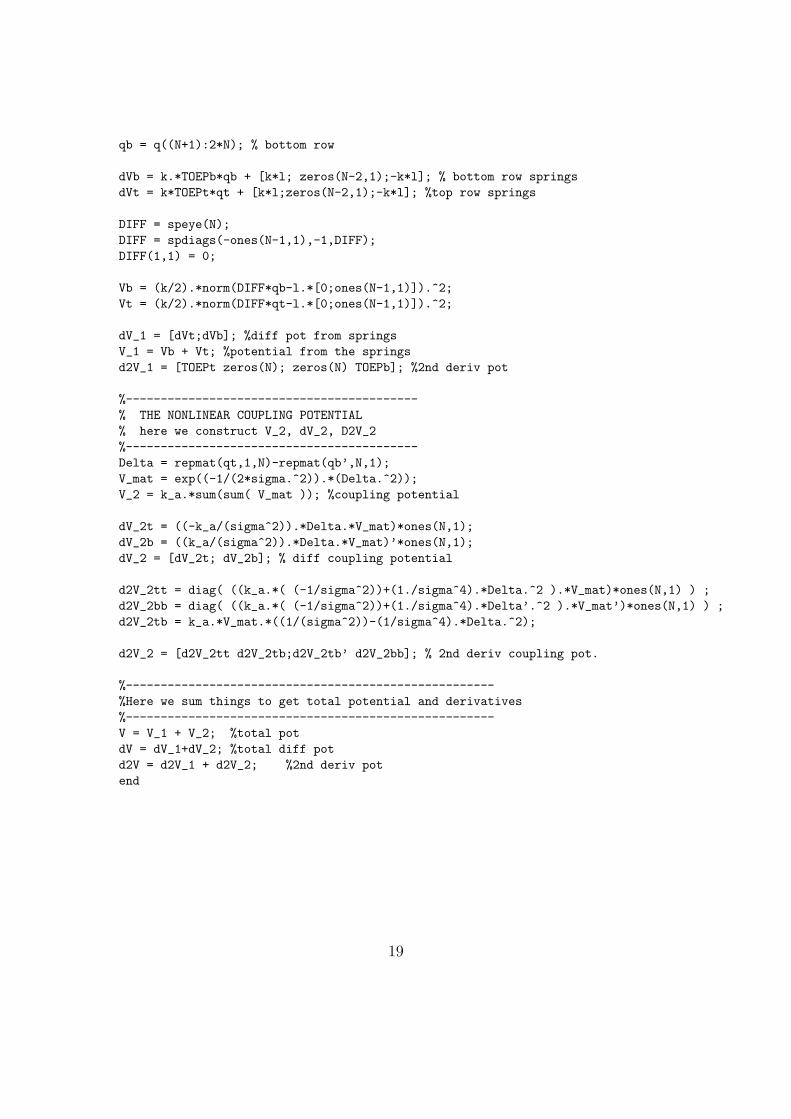
Here’s the program I used to implement the scheme outlined in section 2.

function [q,t,K,K_b,K_t,V,V_b,V_t,p_b,p_t] = model11(v0)% Simulates two Hookean mass spring chains with% a nonlinear coupling between each other. The% positions of the masses are stored in the vector q.

global N l k k_a sigmaN = 20;l = 1./N;k = 1.0; % spring constantk_a = 0.001; % coupling (+ for repulsion)sigma = 0.1;mt = 1.0; % mass of springs on topmb = 1.0; % mass of springs below

M = [mt*eye(N) zeros(N);zeros(N) mb*eye(N)]; %mass matrixh = min(2*pi./(10*sqrt(k)),0.1); % time-step sizestep_max = 1000; %number of time steps to implement

% initial conditionsqt0 = (l.*(1:N)’)-3;qt1 = qt0 + h.*v0;qb0 = l.*(1:N)’;qb1 = qb0;% - h.*v0./2;

% initialize qq = zeros(2*N,step_max);q(:,1) = [qt0;qb0];q(:,2) = [qt1;qb1];

% run integratordisplay(’running integrator’)V = zeros(1,step_max-2);V_t = zeros(1,step_max-2);V_b = zeros(1,step_max-2);

K = zeros(1,step_max-2);K_t = K;K_b = K;p_t = K;p_b = K;for ind = 3:step_max

q1 = q(:,ind-1);q0 = q(:,ind-2);q2 = 2*q1-q0;error = 1;

17

while error > 10^(-8)[V1,dV1,d2V1, Vt_1, Vb_1] = potential(0.5.*(q0+q1));[V2,dV2,d2V2, Vt_2, Vb_2] = potential(0.5.*(q2+q1));F = (1./(h^2)).*M*(q2-2.*q1+q0)+0.5.*(dV1+dV2);error = max(abs(F));q2 = q2 - ((1/h^2).*M+0.25*d2V2)\F;

endq(:,ind) = q2;V(ind-2) = 0.5*(V1+V2);V_t(ind-2) = 0.5*(Vt_1+Vt_2);V_b(ind-2) = 0.5*(Vb_1+Vb_2);vel = (q2-q0)./(2*h);K(ind-2) = 0.5.*(vel’*M*vel);vel_t = vel(1:N);p_t(ind-2) = mean(mt*vel_t);K_t(ind-2) = 0.5*mt*(vel_t’*vel_t);vel_b = vel((N+1):(2*N));p_b(ind-2) = mean(mb*vel_b);K_b(ind-2) = 0.5*mb*(vel_b’*vel_b);

endt = h.*(1:(step_max-2))’;store = q;q = store(:,2:(end-1));

display(’done integrating’)beepend

function [V, dV, d2V, Vt, Vb] = potential(q )% [V, dV, d2V, Vt, Vb] = potential(q )% Gives the potential and fist and 2nd derivatives% of the potential function V = V_1 + V_2

global N k k_a l sigma

%--------------------------------------------% HOOKEAN SPRINGS% Here we construct V_1, dV_1, d2V_1% The linear spring potential%--------------------------------------------TOEPb = spalloc(N,N,3*N);TOEPb = spdiags(ones(N,1),0,TOEPb);TOEPb = spdiags(-ones(N-1,1),-1,TOEPb);TOEPb = TOEPb+TOEPb’; % Toeplitz MatrixTOEPb(1,1) = 1;TOEPb(N,N) = 1;TOEPt = TOEPb;

qt = q(1:N); % top row

18

qb = q((N+1):2*N); % bottom row

dVb = k.*TOEPb*qb + [k*l; zeros(N-2,1);-k*l]; % bottom row springsdVt = k*TOEPt*qt + [k*l;zeros(N-2,1);-k*l]; %top row springs

DIFF = speye(N);DIFF = spdiags(-ones(N-1,1),-1,DIFF);DIFF(1,1) = 0;

Vb = (k/2).*norm(DIFF*qb-l.*[0;ones(N-1,1)]).^2;Vt = (k/2).*norm(DIFF*qt-l.*[0;ones(N-1,1)]).^2;

dV_1 = [dVt;dVb]; %diff pot from springsV_1 = Vb + Vt; %potential from the springsd2V_1 = [TOEPt zeros(N); zeros(N) TOEPb]; %2nd deriv pot

%------------------------------------------% THE NONLINEAR COUPLING POTENTIAL% here we construct V_2, dV_2, D2V_2%------------------------------------------Delta = repmat(qt,1,N)-repmat(qb’,N,1);V_mat = exp((-1/(2*sigma.^2)).*(Delta.^2));V_2 = k_a.*sum(sum( V_mat )); %coupling potential

dV_2t = ((-k_a/(sigma^2)).*Delta.*V_mat)*ones(N,1);dV_2b = ((k_a/(sigma^2)).*Delta.*V_mat)’*ones(N,1);dV_2 = [dV_2t; dV_2b]; % diff coupling potential

d2V_2tt = diag( ((k_a.*( (-1/sigma^2))+(1./sigma^4).*Delta.^2 ).*V_mat)*ones(N,1) ) ;d2V_2bb = diag( ((k_a.*( (-1/sigma^2))+(1./sigma^4).*Delta’.^2 ).*V_mat’)*ones(N,1) ) ;d2V_2tb = k_a.*V_mat.*((1/(sigma^2))-(1/sigma^4).*Delta.^2);

d2V_2 = [d2V_2tt d2V_2tb;d2V_2tb’ d2V_2bb]; % 2nd deriv coupling pot.

%-----------------------------------------------------%Here we sum things to get total potential and derivatives%-----------------------------------------------------V = V_1 + V_2; %total potdV = dV_1+dV_2; %total diff potd2V = d2V_1 + d2V_2; %2nd deriv potend

19

10 References

[1] J. E. Marsden & T. S. Ratiu, “Introduction to Mechanics and Symmetry: 2ndEdition”, Springer, NY, 1999

[2] M. West, “Variational Integrators”, Caltech, 2004

[3] O.M. Braun & Y.S. Kivshar, “The Frenkel-Kontorova Model”, Springer,NY 2003

[4] R.C. Tolman, “The Principles of Statistical Mechanics”, Dover, 1980

20