Money DemandECON 40364: Monetary Theory & Policy

Eric Sims

University of Notre Dame

Spring 2020

1 / 38

Readings

I Mishkin Ch. 19

2 / 38

Classical Monetary Theory

I We have now defined what money is and how the supply ofmoney is set

I What determines the demand for money?

I How do the demand and supply of money determine the pricelevel, interest rates, and inflation?

I We will focus on a framework in which money is neutral andthe classical dichotomy holds: real variables (such as outputand the real interest rate) are determined independently ofnominal variables like money

I We can think of such a world as characterizing the “medium”or “long” runs (periods of time measured in several years)

I We will soon discuss the “short run” when money is notneutral

3 / 38

Velocity and the Equation of Exchange

I Let Yt denote real output in period t, which we can take tobe exogenous with respect to the money supply

I Pt is the dollar price of output, so PtYt is the dollar value ofoutput (i.e. nominal GDP)

I 1Pt

is the “price” of money measured in terms of goods

I Define velocity as as the average number of times per yearthat the typical unit of money, Mt , is spent on goods andserves. Denote by Vt

I The “equation of exchange” or “quantity equation” is:

MtVt = PtYt

I This equation is an identity and defines velocity as the ratio ofnominal GDP to the money supply

4 / 38

From Equation of Exchange to Quantity Theory

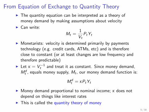
I The quantity equation can be interpreted as a theory ofmoney demand by making assumptions about velocity

I Can write:

Mt =1

VtPtYt

I Monetarists: velocity is determined primarily by paymentstechnology (e.g. credit cards, ATMs, etc) and is thereforeclose to constant (or at least changes are low frequency andtherefore predictable)

I Let κ = V−1t and treat it as constant. Since money demand,Md

t , equals money supply, Mt , our money demand function is:

Mdt = κPtYt

I Money demand proportional to nominal income; κ does notdepend on things like interest rates

I This is called the quantity theory of money

5 / 38

Money and Prices

I Take natural logs of equation of exchange:

lnMt + lnVt = lnPt + lnYt

I If Vt is constant and Yt is exogenous with respect to Mt ,then:

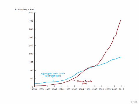
d lnMt = d lnPt

I In other words, a change in the money supply results in aproportional change in the price level (i.e. if the money supplyincreases by 5 percent, the price level increases by 5 percent)

6 / 38

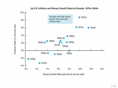
Money and Inflation

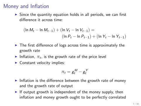
I Since the quantity equation holds in all periods, we can firstdifference it across time:

(lnMt − lnMt−1) + (lnVt − lnVt−1) =

(lnPt − lnPt−1) + (lnYt − lnYt−1)

I The first difference of logs across time is approximately thegrowth rate

I Inflation, πt , is the growth rate of the price level

I Constant velocity implies:

πt = gMt − gY

t

I Inflation is the difference between the growth rate of moneyand the growth rate of output

I If output growth is independent of the money supply, theninflation and money growth ought to be perfectly correlated

7 / 38

8 / 38

9 / 38

10 / 38

Nominal and Real Interest Rates

I The nominal interest rate tells you what percentage of yournominal principal you get back (or have to pay back, in thecase of borrowing) in exchange for saving your money. Denoteby it

I There are many interest rates, differing by time to maturityand risk. Ignore this for now. Think about one period(riskless) interest rates – i.e. between t and t + 1

I The real interest rate tells you what percentage of a good youget back (or have to pay back, in the case of borrowing) inexchange for saving a good. Denote by rt

I Putting one good “in the bank” ⇒ Pt dollars in bank ⇒(1 + it)Pt dollars tomorrow ⇒ purchases (1 + it)

PtPt+1

goodstomorrow

11 / 38

The Fisher Relationship

I The relationship between the real and nominal interest rate isthen:

1 + rt = (1 + it)Pt

Pt+1

I Since the inverse of the ratio of prices across time is theexpected gross inflation rate, we have:

1 + rt =1 + it

1 + πet+1

I Here πet+1 is expected inflation between t and t + 1

I Approximately:rt = it − πe

t+1

12 / 38

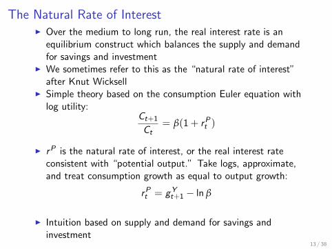
The Natural Rate of InterestI Over the medium to long run, the real interest rate is an

equilibrium construct which balances the supply and demandfor savings and investment

I We sometimes refer to this as the “natural rate of interest”after Knut Wicksell

I Simple theory based on the consumption Euler equation withlog utility:

Ct+1

Ct= β(1 + rPt )

I rP is the natural rate of interest, or the real interest rateconsistent with “potential output.” Take logs, approximate,and treat consumption growth as equal to output growth:

rPt = gYt+1 − ln β

I Intuition based on supply and demand for savings andinvestment

13 / 38

Money, Inflation, and Interest Rates

I Over the medium to long run, the natural rate of interest justdepends on output growth and attitudes about saving,captured by β. Independent of monetary factors. Think ofthis as constant.

I Over the medium to long run, we should also expect expectedinflation to equal realized inflation, πe

t+1 = πt

I From the Fisher relationship, this means that nominal interestrates and inflation ought to move together

14 / 38

0

2

4

6

8

10

12

14

16

0 2 4 6 8 10

1955

19561957

1958

19591960

19611962

19631964

1965

19661967

1968

19691970

19711972

19731974

197519761977

1978

1979

1980

1981

1982

1983

1984

1985

19861987

1988

19891990

1991

19921993

1994

19951996199719981999

2000

2001

20022003

2004

2005

20062007

2008

20092010 201120122013201420152016

Inflation Rate

Thre

e M

onth

Tre

asur

y B

ill R

ate

Correlation = 0.74

15 / 38

Theoretical Predictions

I The basic quantity theory in which the classical dichotomyholds (real output, real output growth, and the real interestrate independent of nominal things) makes a number of starkpredictions

1. The level of the money supply and the price level are closelylinked

2. The growth rate of the money supply and the inflation rate areclosely linked

3. The inflation rate and the nominal interest rate are closelylinked

16 / 38

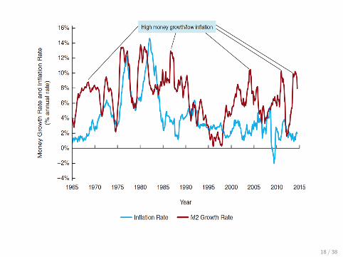
Problems with the Quantity Theory

I The quantity theory seems to provide a pretty good theory ofinflation and interest rates over the medium to long run aswell as in a cross section of countries

I What about the short run?I Problems with the quantity theory:

I The shorter term relationships between money growth andboth inflation and nominal interest rates are weak

I Velocity is not constant and has become harder to predict,particularly since the early 1980s

17 / 38

18 / 38

19 / 38

20 / 38

21 / 38

Moving Beyond the Quantity TheoryI The key assumption in the quantity theory is that the demand

for money (i.e. velocity) is stable (or at least predictable) –you hold money to buy stuff, and how much money you needis proportional to how much you buy

I Liquidity preference theory of money demand: moneycompetes with other assets as a store of value. Money is moreliquid (can be used in exchange), but how much you want tohold depends on return on other assets

I Demand for real money balances, mt =MtPt

, is an increasingfunction of output, Yt , but a decreasing function of thenominal interest rate, it :

Mt

Pt= L(it

−,Yt+)

I But then velocity:

Vt =PtYt

Mt=

Yt

L(it ,Yt)

22 / 38

Money in the Utility Function

I Suppose that there is a representative household who receivesutility from consuming goods and holding real moneybalances, mt =

MtPt

. Flow utility:

U

(Ct ,

Mt

Pt

)= lnCt + ψ ln

(Mt

Pt

)

I Flow budget constraint:

PtCt + Bt − Bt−1 +Mt −Mt−1 ≤ PtYt − PtTt + it−1Bt−1

I Bt−1 and Mt−1: stocks of bonds and money household enterst with

I Both enter as stores of value. Difference being that bonds payinterest

I Household discounts future utility flows by β ∈ [0, 1)

23 / 38

Optimality Conditions

I Plugging constraints in and taking derivatives yields:

1

Ct= βEt

1

Ct+1(1 + it)

Pt

Pt+1

ψPt

Mt=

1

Ct− βEt

1

Ct+1

Pt

Pt+1

I Government’s budget constraint with Gt = 0 (ignoredistinction between base and money supply):

PtTt = (1 + it)BG ,t−1 − BG ,t − (Mt −Mt−1)

I Market-clearing: BG ,t = Bt , so Ct = Yt

24 / 38

Money Demand Function

I Making use of market-clearing and combining the FOC yields:

ψm−1t =1

Yt

it1 + it

I Re-arranging:

mt = ψYt1 + itit

I Demand for real balances: (i) increasing in Yt , (ii) decreasingin it

I Zero lower bound: must have it ≥ 0 to get non-negative realbalances. At it → 0, demand for real balances goes to infinity

25 / 38

Baumol-Tobin

I You need to spend Y over the course of a period (say, a year)

I You keep wealth “in the bank” earning nominal interest it(say a savings account, not demand deposit)

I You need to determine how many trips you take to bank

I Each trip incurs a cost (“shoeleather cost”) of K

I Let mt denote average real balances holdings over the period.Opportunity cost of holding money is itmt

I Each time you withdraw money, you withdraw 2mt dollars.Total trips to bank is Y

2mt

I Objective is to pick mt to minimize:

minmt

itmt +KY

2mt

26 / 38

Money Demand Function

I Use calculus to get first order condition:

mt =

√KYt

2it

I Or re-arranging:

mt =

(KYt

2

) 12

i− 1

2t

I Demand for real balances again increasing in Yt anddecreasing in it

I There is again a zero lower bound: it ≥ 0 for demand for realbalances to be positive

27 / 38

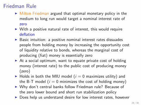
Friedman RuleI Milton Friedman argued that optimal monetary policy in the

medium to long run would target a nominal interest rate ofzero

I With a positive natural rate of interest, this would requiredeflation

I Basic intuition: a positive nominal interest rates dissuadespeople from holding money by increasing the opportunity costof liquidity relative to bonds, whereas the marginal cost ofproducing (fiat) money is essentially zero

I At a social optimum, want to equate private cost of holdingmoney (interest rate) to the public cost of producing money(zero)

I Holds in both the MIU model (i = 0 maximizes utility) andthe B-T model (i = 0 minimizes the cost of holding money)

I Why don’t central banks follow Friedman rule? Because ofthe zero lower bound and short run stabilization policy

I Does help us understand desire for low interest rates, however28 / 38

Optimality of i = 0

i0 2 4 6

Aln

m

0

0.5

1

1.5

2MIU Model

i0 2 4 6

i"m

+K

Y2m

0

1

2

3

4B-T Model

29 / 38

Instability of Velocity: Movement Away from Focusing onMonetary Aggregates

I Paul Volcker and the Fed experimented with targetingmonetary aggregates in the early 1980s

I This brought inflation down from the 1970s, but led to highand variable interest rates

I Most monetary economists concluded that the demand formoney is not in fact stable, i.e. a rejection of monetarism

I If the money supply is not closely and predictably connectedto aggregate spending, targeting the money supply probablynot a good policy

I This has led most monetary economists to instead favoringfocusing on short term interest rates as the target of monetarypolicy, as we saw with a discussion of the Taylor rule and theFed controlling the Fed Funds Rate (FFR)

30 / 38

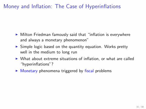
Money and Inflation: The Case of Hyperinflations

I Milton Friedman famously said that “inflation is everywhereand always a monetary phenomenon”

I Simple logic based on the quantity equation. Works prettywell in the medium to long run

I What about extreme situations of inflation, or what are called“hyperinflations”?

I Monetary phenomena triggered by fiscal problems

31 / 38

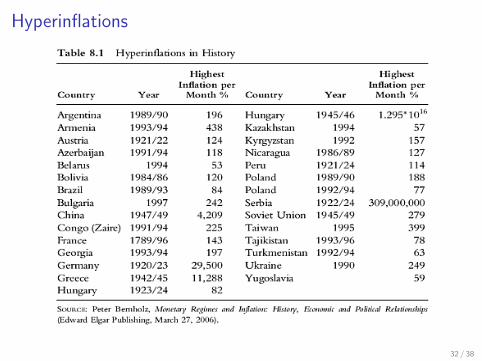
Hyperinflations

32 / 38

Hyperinflations Usually a Fiscal Phenomenon

I Most hyperinflations in history are associated with fiscalmischief

I Government’s budget constraint:

PtGt + it−1BG ,t−1 = PtTt +Mt −Mt−1 + BG ,t − BG ,t−1

I Here Pt is the nominal price of goods (i.e. the price level),BG ,t−1 is the stock of debt with which a government entersperiod t, BG ,t is the stock of debt the government takes fromt to t + 1, it−1 is the nominal interest rate on that debt, Tt istax revenue (real), and Mt is the money supply

I Deficit equals change in money supply plus change in debt:

PtGt + it−1BG ,t−1 − PtTt = Mt −Mt−1 + BG ,t − BG ,t−1

33 / 38

Monetizing the Debt

I If tax revenue doesn’t cover expenditure (spending plusinterest on debt), then government either has to issue moredebt or “print more money”

I In some cases printing more money is explicit, in othersimplicit

I Monetizing the debt: fiscal authority issues debt to financedeficit, but monetary authority buys the debt by doing openmarket operations, which creates base money

34 / 38

Application: Seigniorage and the Inflation Tax

I Recall from the government’s budget constraint above whentalking about hyperinflations that nominal revenue fromprinting money is simply: Mt −Mt−1

I Real revenue from printing money is Mt−Mt−1Pt

I We call the real revenue from printing money seigniorage

I This can be written:

Seigniorage =Mt −Mt−1

Pt

I This can equivalently be written:

Seigniorage =Mt −Mt−1

Mt−1

Mt−1Mt

Mt

Pt

35 / 38

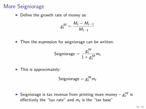
More Seigniorage

I Define the growth rate of money as:

gMt =

Mt −Mt−1Mt−1

I Then the expression for seigniorage can be written:

Seigniorage =gMt

1 + gMt

mt

I This is approximately:

Seigniorage = gMt mt

I Seigniorage is tax revenue from printing more money – gMt is

effectively the “tax rate” and mt is the “tax base”

36 / 38

Seigniorage in the Medium to Long RunI Suppose that the growth rate of money is constant in the

medium to long run, gMt = gM

I Suppose that output, Yt , is independent of the money growthrate and is constant, so Yt = Y

I Suppose that the real interest rate equals the natural rate ofinterest, so the nominal rate is constant and is:

i = rP + π

I Suppose that the inflation rate equals the money growth rate,so:

i = rP + gM

I If demand for real balances is generically given by:mt = L(it ,Yt), then we can write demand for real balances as:

m = L(rP + gM ,Y )

37 / 38

“Optimal” Inflation TaxI Suppose that a central bank wants to pick gM to maximize

seigniorage. Problem is:

maxgM

gML(rP + gM ,Y )

I Provided money demand is decreasing in nominal interest rate(i.e. Li (·) < 0), then two competing effects of higher gM :

1. Tax rate: higher gM ⇒ higher tax rate2. Base: higher gM ⇒ lower tax base

I First order condition:

gM = − L(rP + gM ,Y )

Li (rP + gM ,Y )

I Revenue-maximizing growth rate of money inversely related tointerest sensitivity of money demand

I If money demand interest insensitive (e.g. quantity theory),then revenue-maximizing gM = ∞!

I Desire for seigniorage another reason to move away fromFriedman rule

38 / 38