mr image super-resolution reconstruction using sparse representation, nonlocal...

MR image super-resolution reconstruction using sparse representation,nonlocal similarity and sparse derivative prior

Di Zhang a,c,n, Jiazhong He b, Yun Zhao a, Minghui Du c

a School of Information Engineering, Guangdong Medical College, Dongguan, Chinab Department of Physics, Shaoguan University, Shaoguan, Chinac School of Electronics and Information, South China University of Technology, Guangzhou, China

a r t i c l e i n f o

Article history:Received 29 June 2014Accepted 30 December 2014

Keywords:Magnetic resonance imagingSuper-resolutionSparse representationSparse derivative priorNonlocal similarity

a b s t r a c t

In magnetic resonance (MR) imaging, image spatial resolution is determined by various instrumentallimitations and physical considerations. This paper presents a new algorithm for producing a high-resolution version of a low-resolution MR image. The proposed method consists of two consecutivesteps: (1) reconstructs a high-resolution MR image from a given low-resolution observation via solving ajoint sparse representation and nonlocal similarity L1-norm minimization problem; and (2) applies asparse derivative prior based post-processing to suppress blurring effects. Extensive experiments onsimulated brain MR images and two real clinical MR image datasets validate that the proposed methodachieves much better results than many state-of-the-art algorithms in terms of both quantitativemeasures and visual perception.

& 2015 Elsevier Ltd. All rights reserved.

1. Introduction

Compared with other medical imaging techniques, MR imaginguses non-ionizing radiation and provides distinct microscopicchemical and physical information of molecules. However, thespatial resolution of MR images is limited by various instrumentallimitations (e.g., gradients’ intensity, filter bandwidth) and physi-cal considerations. The resolution limitation could result in partialvolume effect (PVE), a phenomenon that each pixel in the MRimages could contain more than one material or tissue type. Toreduce PVEs, a common practice is to magnify the images usingstandard interpolation techniques. However, interpolation techni-ques usually do not take into account the fact that a low-resolution(LR) pixel is actually a weighted average of the high-resolution(HR) pixels inside it, thus the magnified HR images are typicallyfeatured with blurred edges and tissues.

To overcome this problem, various methods have been pro-posed [1,5–8,11,12,17–20] so far. Among them, super-resolution(SR) is one of the most promising methods and receives muchattention in the research community. SR image reconstruction isthe process of recovering a HR image from a single (e.g., [2])or a set of LR images (e.g., [3]). The essential difference between

single-frame and multi-frame SR image reconstruction is that newhigh-frequency information could also be recovered from differentLR frames [4]. In MR image analysis, SR was first used toreconstruct a HR image by merging multiple LR acquisitions withsubpixel displacements. In [5], Herment et al. reduced total dataacquisition time by merging multiple k-space data. Shilling et al.[6] improved the resolution and contrast of MR images by fusingmultiple 2D slices with different slice directions. Greenspan et al.[7] used iterative back-projection and Islamet al. [8] used awavelet-based deblurring approach to improve the resolution of3D MR images.

Though multi-frame SR image reconstruction is theoreticallymore promising than single-frame SR image reconstruction, itsuffers many difficulties in real applications, such as subpixelimage registration/acquisition, the increase of computational com-plexity as frame number increases. On the other hand, manyresearches [9,10] have demonstrated that, given a proper priorimage model, single-frame SR image reconstruction can also be aseffective as multi-frame SR image reconstruction. To reconstruct aHR image from a single MR image, Rousseau [11] used the ideapresented in [9] and proposed a patch-based nonlocal regulariza-tion framework for brain MR image reconstruction. Manjón et al.[12] extended the patch-based nonlocal regularization frameworkto include a coherence constraint.

Recently, a powerful statistical image modeling technique,sparse representation [13,14], has been successfully applied innatural image SR applications [15,16,22]. In MR image analysis,

Contents lists available at ScienceDirect

journal homepage: www.elsevier.com/locate/cbm

Computers in Biology and Medicine

http://dx.doi.org/10.1016/j.compbiomed.2014.12.0230010-4825/& 2015 Elsevier Ltd. All rights reserved.

n Corresponding author at: Guangdong Medical College, School of InformationEngineering, Song Shan Hu, Dongguan, China. Tel./fax: þ86 20 3876 9529.

E-mail address: [email protected] (D. Zhang).

Computers in Biology and Medicine 58 (2015) 130–145

www.sciencedirect.com/science/journal/00104825

www.elsevier.com/locate/cbm

http://dx.doi.org/10.1016/j.compbiomed.2014.12.023



http://crossmark.crossref.org/dialog/?doi=10.1016/j.compbiomed.2014.12.023&domain=pdf



mailto:[email protected]


however, many efforts have been focused on applying compressedsensing (CS) [17–20], a technique through which a perfect MRimage reconstruction is possible by only a small subset of k-spacesamples that is far less than the Nyquist sampling theorem. Sincethese CS-based SR methods [17–20] focus on manipulating k-spacesamples, they do have many advantages, e.g., theoretical simplicityand low computational cost. Nevertheless, they also present someimportant drawbacks. For example, recovering high frequencyinformation in the k-space will inevitably cause visual artifactsin the image space, thus they need to work in the frequency andthe image space in turn to suppress artifacts [20,21]. On the otherhand, sparse representation based techniques manipulate imagepatches in the image space, thus provide much more interpretableinformation to human eyes, and more importantly, facilitateexperts to adopt a much more flexible observation model (e.g.,local motion) and incorporate various image priors. Based on theseconsiderations, Andrea et al. [21] proposed to reconstruct HR 3Dbrain MR image from LR 3D image volumes using overcompletedictionaries.

Motivated by the ideas presented in Refs. [11,12,21,36,37], inthis paper, we propose a new algorithm for reconstructing a HRMR image from a single LR image. The proposed method consistsof two consecutive steps: (1) reconstructs a HR MR image from agiven LR observation via solving a joint sparse representation andnonlocal similarity L1-normminimization problem; and (2) appliesa sparse derivative prior based post-processing on the recon-structed HR image to suppress blurring effects.

The rest of the paper is organized as follows. In Section 2, wegive a brief review of SR image reconstruction based on sparserepresentation. Sections 3 and 4 present the nonlocal similarityand sparse derivative prior image model, respectively. Section 5presents the new algorithm. Extensive experiments on simulatedbrain MR images and two real clinical MR image datasets areconducted in Section 6 to verify the efficiency of our method.Finally, we provide discussion in Section 7.

2. SR image reconstruction based on sparse representation

In SR image reconstruction, the LR image can be modeled as adown-sampled version of the HR image which has been blurred,i.e.,

Y ¼ WZ ð1Þwhere Y is the observed LR image, Z is the original HR image, andW is a degradation operator representing the blur and down-sampling operator which operates on Z to yield Y (geometric shiftis not included in W since we focus on the single-frame SRreconstruction). A maximum a posterior (MAP) estimate of theunknown HR image Z can be computed as

Z¼ arg maxZ

f log PrðZjYÞg

¼ arg minZ

‖Y�WZ‖22 � log PrðZÞ� � ð2Þ

where Pr(Z) is the prior image model. Many works have beencontributed to find a good prior image model, and total variation(TV) [23–26] is one of the most commonly used models. Sparserepresentation has also been successfully applied as a prior imagemodel as well. Given an image Z, the sparse representationassumes that there exists a sparse vector Λ and a proper learneddictionary Ψ (each column in Ψ is referred to as an atom), suchthat

Z�ΨΛ; s:t: ‖Λ‖0rε ð3Þwhere ε is a predefined threshold to control the sparsity of Λ andL0-norm ‖U‖0 counts the number of nonzero elements in a vector.

Let Ψh and Ψl are the coupled two dictionaries for the HR andLR images, respectively. For single-frame SR reconstruction, givena HR image Z and the corresponding LR image Y, there exists asparse vector Λ simultaneously satisfies [15]

Z�ΨhΛ and Y�ΨlΛ; s:t: ‖Λ‖0rε; ð4ÞWith the sparsity prior image model defined in (4), finding the

solution to (1) is equivalent to finding the representation of Z overΨh, which can be estimated from its LR observation Y by solvingthe following L0-norm minimization problem:

Λ¼ arg minΛ

‖Y�ΨlΛ‖22þλ‖Λ‖0� � ð5Þ

where λ is a parameter controlling the importance of sparsityprior. Since L0-norm is nonconvex and solving (5) is NP-hard,many recent works [13,27] demonstrated that if the coefficients Λis sparse enough, the solution to (5) can be efficiently approxi-mated by solving the following L1-norm minimization problem

Λ¼ arg minΛ

‖Y�ΨlΛ‖22þλ‖Λ‖1� � ð6Þ

where L1-norm ‖U‖1 calculates the sum of the absolute of eachelement in a vector. Notice that (6) is also known as the Lasso instatistical literature [28].

Once Λ is obtained, Z can then be estimated as

Z¼ΨhΛ ð7ÞTraditionally, we divide an image into overlapped or non-

overlapped patches, apply (6) and (7) to each image patch andfuse all the reconstructed HR patches to get the final HR image.To avoid confusion, we use letters in lowercase or uppercase torepresent an image patch or an entire image throughout this paperunless otherwise stated. For the convenience of later discussion,we write the patch-based version of (6) and (7) as follows:

α¼ arg minα

‖y�Ψlα‖22þλ‖α‖1� � ð8Þ

z¼Ψhα ð9Þ

3. Nonlocal similarity

A critical issue in sparse representation prior is the choice ofdictionaries. In general, the more redundant the dictionary is, thebetter SR result will be. Unfortunately, the computational com-plexity will also increase as the size of dictionary increases. Manydictionary learning algorithms thus aim at getting a compact over-complete dictionary to represent various image patches. Never-theless, due to the diversity of natural image patterns, it isimpossible for such compact dictionary to cover all the patterns.As a result, the similar patterns can well be reconstructed whilethe dissimilar ones cannot. Considering the fact that either similaror dissimilar patterns, there are often many repetitive patternsthroughout an image, such nonlocal redundancy is very helpful inpreserving edge sharpness and suppressing noise in the recon-structed images [12,14,29,30]. As a supplementary to the sparserepresentation prior, in this section, we will develop a nonlocalsimilarity regularization term for SR image reconstruction.

For a given image patch zj, we search for the similar patcheswithin a sufficiently large area around zj. Two similarity criteriahave been frequently used so far: (1) a patch zsj is selected as asimilar patch to zj if dsj ¼ j jzsj �zj j j 22rt, where t is a presetthreshold, or (2) one can select the patch if it is within the first L(e.g., L¼15) closest patches to zj. However, they are all based onEuclidean norm in the vector space and do not truly reflect the

D. Zhang et al. / Computers in Biology and Medicine 58 (2015) 130–145 131

similarity between two vectors. In this paper, we use the cosine ofthe angle between two vectors as the distance measurement,

dsj ¼zsj ; zjD E

ðj jzsj j j 2 U j jzj j j 2Þð10Þ

Suppose L similar patches (zsj , s¼1,2,…,L) have been located forzj, let zsj be the central pixel of zsj and zj be the central pixel of zj.We can use the weighted average of zsj to predict zj,

zj ¼XL

s ¼ 1zsj c

sj ð11Þ

where csj is the weight assigned to zsj , determined by

csj ¼expð�dsj =hÞPL

s ¼ 1 expð�dsj =hÞð12Þ

where dsj is determined by (10) and h is a controlling factor of theweight. Considering the fact that there are plenty of repetitivepatterns throughout a MR image, the mean squared error betweenthe prediction and the ground truth, i.e.,

j j zj� zj j j 22 ¼ j j zj�XL

s ¼ 1zsj c

sj j j 22 ð13Þ

should be sufficiently small. Let cj be the column vector containingall the weights csj and patch pj be the column vector containing allzsj . By summing the mean squared prediction error across thewhole image patch zj, we get

Xzj Azj

j j zj�XL

s ¼ 1zsj c

sj j j 22 ¼

Xzj Azj

j j zj�cTj pj j j 22 ð14Þ

Since (8) calculates the sparse representation coefficients of HRimage patch z only using fidelity constraint and sparsity prior, toincorporate the nonlocal similarity regularization, we revise (8) asfollows:

α¼ arg minα

‖y�Ψlα‖22þλ‖α‖1þηXzj A zj

j j zj�cTj pj j j 22

8<:

9=; ð15Þ

where η is a parameter controlling the contribution of nonlocalsimilarity regularization. If we define a matrix C as

Cjs ¼csj ; ifz

sj Apj; c

sj Acj

0;otherwise

(ð16Þ

By substituting (16) and z¼Ψlα into (15), we get

α¼ arg minα

‖y�Ψlα‖22þλ‖α‖1þηj j ðI�CÞΨlαj j 22� � ð17Þ

where I is an identity matrix. By introducing

yn ¼ y0

� �and Γ¼

IηðI�CÞ

" #ð18Þ

Eq. (17) can further be simplified as

α¼ arg minα

‖yn�ΓΨlα‖22þλ‖α‖1� � ð19Þ

Please note that (19) has exactly the same form of (8), which isalso a L1-norm minimization problem.

4. Sparse derivative prior image model

Compared with the TV model, using sparsity prior or nonlocalsimilarity can improve the quality of the final HR image. However, we

will demonstrate in Section 6 that sparsity prior or nonlocalsimilarity based methods also produce blurry effects along strongedges or in soft tissue areas in the reconstructed MR images. Ingeneral, the blurry effect is caused by the average operation in thesemethods. For sparsity prior based methods, overlapped HR patchesare separately reconstructed and the pixels in the overlapped regionsare averaged via various strategies to maintain compatibility betweenadjacent patches, and as a result, the selected averaging strategylargely determines the blurry degree. On the other hand, for nonlocalsimilarity based methods, L similar patches (not identical patches)are averaged to predict the central pixel of the target patch, andcertainly the higher the degree of similarity, the less blurry effect inthe final HR MR image. Since balancing the blurry effect of sparsityprior and nonlocal similarity under a unified L1-norm minimizationframework is difficult and complicated, in this paper, we adopt thesparse derivative prior image model to suppress blurry effects.

For lots of natural images, researchers have found that afterapplying a localized, oriented, and bandpass filtering operation, thehistogram of the filtered images are exponential with high fourth-order statistics (kurtosis) [38–40]. For example, Fig. 1(a) shows anatural image, the histogram of the filtered image via a 1-D filter [�1,0, 1] is shown in Fig. 1(b). We canmodel the distribution in Fig. 1(b) via

PrðxÞp exp �12

jxjσ

� �α� �ð20Þ

where σ is the standard deviation, and α is the exponent parameter.Fig. 1(b) reveals the fact that the gradients of an image are largelyzeros, i.e., strong derivatives are sparse in a given natural image. Eq.(20) is also known as the natural image prior when 0oαo1, for itcan model lots of natural images [38–40]. Unlike the TV modelassumes local smoothness, the natural image prior tends to encou-rage a single strong derivative, which would appear as a sharp edgein local regions. The natural image prior has been successivelyapplied in natural image noise reduction [41], compression [42],deconvolution [43,44], and SR as well [36,37]. In [37], Tappen et al.simultaneously used fidelity constraint and natural image prior toperform SR. Kwang and Younghee [36] first used kernel ridgeregression and then applied natural image prior based post-processing to suppress ringing artifacts. Nevertheless, to the authors’best knowledge, by far there are many works reported on naturalimage processing utilizing natural image prior, little similar job wasdone on MR images or other medical images. To validate whether thenatural image prior can be applied to MR images, we filter a brain MRimage (shown in Fig. 2(a)) with the same 1-D filter used in Fig. 1 andshow the histogram of the filtered image in Fig. 2(b). By comparingFig. 1 with Fig. 2, it is clear that though the two images shown inFig. 1(a) and Fig. 2(a) are quite different in nature, the distributionsare almost the same, which implies that the natural image prior canalso be used in MR image processing.

In [37], Tappen et al. estimated the HR patch z by maximizingthe following joint posterior probability distribution

Prð zf gj y� �Þ ¼ 1

C∏

j; iAN8ðjÞexp � ‖zj�zi‖1

σN

� �α� �∏jexp � ‖Wzj�yj‖2

σR

� �2" #

ð21Þ

where {y} denotes the observed variables corresponding to thepixels in LR image Y, {z} represents the latent variables corre-sponding to the patch in HR image Z which satisfies y¼Wz, N8(j)denotes for 8-connected neighbors of the pixel at location j, C isthe normalization constant, σN and σR are standard deviationparameters. The first product in (21) is the natural image priorterm and the second one is the fidelity constraint term. Consider-ing that the data fidelity constraint has already been incorporatedin the reconstruction process via the coupled two dictionaries Ψh

D. Zhang et al. / Computers in Biology and Medicine 58 (2015) 130–145132

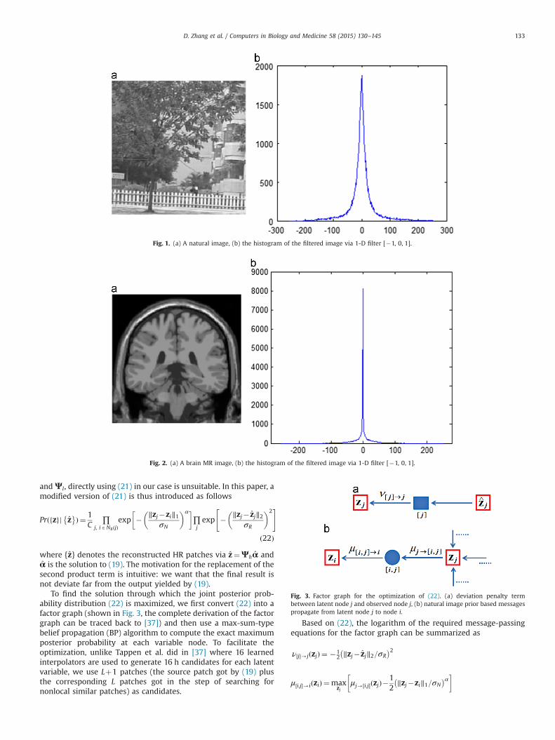
andΨl, directly using (21) in our case is unsuitable. In this paper, amodified version of (21) is thus introduced as follows

Prð zf gj z� �Þ ¼ 1

C∏

j; iAN8ðjÞexp � ‖zj�zi‖1

σN

� �α� �∏jexp � ‖zj� zj‖2

σR

� �2" #

ð22Þ

where {z} denotes the reconstructed HR patches via z¼Ψhα andα is the solution to (19). The motivation for the replacement of thesecond product term is intuitive: we want that the final result isnot deviate far from the output yielded by (19).

To find the solution through which the joint posterior prob-ability distribution (22) is maximized, we first convert (22) into afactor graph (shown in Fig. 3, the complete derivation of the factorgraph can be traced back to [37]) and then use a max-sum-typebelief propagation (BP) algorithm to compute the exact maximumposterior probability at each variable node. To facilitate theoptimization, unlike Tappen et al. did in [37] where 16 learnedinterpolators are used to generate 16 h candidates for each latentvariable, we use Lþ1 patches (the source patch got by (19) plusthe corresponding L patches got in the step of searching fornonlocal similar patches) as candidates.

Based on (22), the logarithm of the required message-passingequations for the factor graph can be summarized as

ν½j�-jðzjÞ ¼ �12 ‖zj� zj‖2=σR� 2

μ½i;j�-iðziÞ ¼maxzj

μj-½i;j�ðzjÞ�12

‖zj�zi‖1=σN� α� �

Fig. 2. (a) A brain MR image, (b) the histogram of the filtered image via 1-D filter [�1, 0, 1].

Fig. 3. Factor graph for the optimization of (22). (a) deviation penalty termbetween latent node j and observed node j, (b) natural image prior based messagespropagate from latent node j to node i.

Fig. 1. (a) A natural image, (b) the histogram of the filtered image via 1-D filter [�1, 0, 1].


μj-½i;j�ðzjÞ ¼ ν½j�-jðzjÞþX

kAN8ðjÞ\iμ½j;k�-jðzjÞ ð23Þ

where ν½j�-j calculates the message sent from constraint node [j] tovariable node zj, μ½i;j�-i represents the message sent from con-straint node [i,j] to variable node zi, and μj-½i;j� is the message sentfrom variable node j to constraint node [i,j]. In (23), μj-½i;j� andμ½i;j�-i are natural image prior based messages propagate fromlatent node j to node i, while ν½j�-j is the deviation penalty termbetween latent node j and observed node j.

With Lþ1 candidate HR patches in hand, the sparse derivativeprior based post-processing is summarized in Algorithm 1.

Algorithm 1.

(1) Run BP algorithm X times using the three message-passingequations defined in (23).

(2) For each variable node zj, select the candidate HR patch withthe highest belief.

(3) Insert the selected candidate HR patches into the correspond-ing position to form the final output HR image.

5. The proposed method

In this section, we first discuss how to construct the coupled HRand LR dictionaries, and then propose a new SR algorithm toreconstruct a HR image from a single LR MR image.

5.1. Dictionary construction

In this paper, we use a modified version of the methodpresented in [15,21] to construct the coupled two dictionariesΨh and Ψl (as illustrated in Fig. 4). Each HR training image in thetraining set {Zj, j¼1,2,…, N} is first blurred and down-sampled by afactor of q to produce the corresponding LR image set {Yj, j¼1,2,…,N} (i.e., Yj¼WZj, where W is the degradation operator defined in(1)). Then a upsampled set {YU

j , j¼1,2,…, N} is obtained by scalingeach image in {Yj} by the same factor q via bicubic interpolation(i.e., YU

j ¼UqYj, where Uq is the bicubic interpolator with amagnification factor of q). Since we want dictionary Ψh containsuseful discriminative high-frequency information, the original HRtraining set {Zj} is further processed to obtain an updated HRtraining set {ZU

j ; j¼1,2,…, N} via ZUj ¼ Zj�YU

j . For dictionary Ψl,many previous work demonstrated that building it in featurespace is more suitable than in image space [15,16,21]. Consideringthe fact that the high-frequency information of the LR image iscritical for predicting the lost high-frequency information in thetarget HR image, people often choose the feature space as somekind of high-pass filtered image. For example, Yang et al. [15] usedthe first- and second-order derivatives as the feature due to theirsimplicity and effectiveness, Rueda et al. [21] applied a multi-scaleedge analysis, where a series of 6 different filters (Sobel kernels,size 3�3�3 and 5�5�5, in x, y and z directions) are used. To

combine the merits of both multi-scale analysis and the first- andsecond-order derivatives, in this paper, we use a multi-scale (size3�3 and 5�5) first- and second-order derivative analysis toextract features from the upsampled image set {YU

j }.The eight 1-D filters used to extract multi-scale first- and

second-order derivatives are

F11 ¼ ½�1;0;1�; F12 ¼ ½�1;0;1�T ; F13 ¼ ½�1; �2; 0; 2; 1�;F14 ¼ ½�1; �2; 0; 2; 1�T

F21 ¼ ½1; �2;1�; F22 ¼ ½1; �2;1�T ; F23 ¼ ½1; 0; �2; 0; 1�;F24 ¼ ½1; 0; �2; 0; 1�T ð24Þwhere F1i and F2i (i¼1 to 4) are the first- and second-orderderivative filters, respectively. For each image in the upsampledimage set {YU

j }, applying these eight filters we obtain eightdifferent filtered images {FriY

Uj , r¼1,2 and i¼1 to 4}.

Following the preprocessing steps described hereinbefore, foreach updated HR training image ZU

j , we now have eight differentfiltered LR images {FriY

Uj }. The procedure for constructing diction-

aries Ψh and Ψl are thus summarized as follows:

1. At each location d of the updated HR training image ZUj , extract

a patch pdZ of size m�m.

2. Extract the corresponding LR patches of the same size from theeight filtered images {FriY

Uj , r¼1,2 and i¼1 to 4} at the same

location. Then concatenate all the eight LR patches to form asingle vector pd

Y of length 8 m2.3. Construct the HR dictionary Ψh and a temporary LR dictionary

Ψn

l by gathering all patches {pdZ} and {pd

Y }, respectively.4. Apply Principal Component Analysis (PCA) to Ψn

l , build thecorresponding orthogonal transformation matrix Q by collect-ing the eigenvectors of the covariance matrix that represents atleast 90% of the original variance.

5. Construct the LR dictionary Ψl via QΨn

l .

The reasonwhy we useΨl instead ofΨn

l as the final LR dictionaryis the redundancy of multi-scale first- and second-order derivativeanalysis, since eight different filters are applied to the same image,resulting in complementary but redundant information.

5.2. Global regularization by back-projection

Since LR dictionary Ψl is not constructed in the original LRimage space, thus the original fidelity constraint ‖y�Ψlα‖22 in theimage space must be replaced by a corresponding constraint in thefeature space, which does not demand exact equality between theLR patch y and its estimation Ψlα. On the other hand, because nocontinuity conditions are imposed along the boundaries betweenpatches, the reconstructed HR image Z4 should thus be furtherrefined to satisfy the SR model (1). To this end, we simply projectZ4 onto the solution space (i.e., Y ¼ WZ[15,21]), computing

Zn ¼ arg minZ

‖Y�WZ‖22þξj jZ� Zj j 22n o

ð25Þ

where ξ is a controlling parameter. Instead of using standardgradient descent method to solve (25), we can iteratively calculatethe difference Y�WZ, convolve it with a back-projection kernel,then warp back into the HR image space to update the estimatedHR image. This process can be written as [15,21,48,49]

Ztþ1 ¼ ZtþðUqðY�WZtÞÞng ð26Þwhere Zt is the estimate of the HR image after the tth iteration, Uq

the bicubic interpolator with a magnification factor of q, g is theback-projection filter and n is the convolution operator. Thisupdating process is iteratively repeated until the differencebetween two consecutive images is less than a given threshold.Fig. 4. Illustration of low- and high-resolution dictionary construction.


5.3. The proposed SR algorithm

With dictionaries Ψh and Ψl, to reconstruct a HR image Z froma given LR image Y, our proposed SR image reconstructionalgorithm (as depicted in Fig. 5) is outlined in Algorithm 2.

Algorithm 2.

1) Upsample the LR image Y using YU ¼UqY2) Perform multi-scale first- and second-order derivative analysis

(i.e., apply the eight 1-D filters defined in (24) to YU to get eightdifferent filtered images {FriY

U , r¼1,2 and i¼1 to 4})3) Divide YU into a grid of nonoverlapping patches with size of

m�m. For each patch y in the image YU, do� Concatenate the patches of the eight filtered images {FriY

U}that correspond to the same location of y to form a patchvector pd

Y� Reduce the dimensionality of pdY via pd

Y ¼QpdY� Substitute pd

Y for y in (18) and solve the optimizationproblem defined in (19)

� Generate the HR patch z via z¼Ψhα� Insert patch z into the corresponding location of the HRimage Z4

4) Update Z using Z¼ ZþYU

5) Use Algorithm 1 to update Z6) Use (26), find the image Zn, which is the closest image to Z that

satisfies the global reconstruction constraint (25)7) Output Zn as the final result of SR image reconstruction

6. Experimental results

6.1. Tested methods

To examine more comprehensively the proposed approach, wetest two versions of the proposed method: one using sparserepresentation prior and nonlocal similarity (denoted by SRNL, step5 is thus excluded from Algorithm 2); the other one using sparserepresentation prior, nonlocal similarity and sparse derivative prior(denoted by SRNINL). To examine the effect of sparse representationprior and nonlocal similarity separately, we test the sparse repre-sentation prior based method proposed by Rueda et al. [21](denoted by SRA) and nonlocal similarity based upsampling [12](denoted by NLUP). Table 1 clearly shows the relation among thesefour methods. On the other hand, two state-of-the-art methods,adaptive sparse domain selection and adaptive regularization(denoted by ASAR) [16], sparse regression and natural image prior(denoted by SRNI) [36], are also tested. Moreover, for a clearcomparison among the above mentioned six methods, we alsoprovide the results yielded by two baseline techniques, i.e., bicubicinterpolation (denoted by SBI) and TV prior [23] (denoted by TV).

Since SRA and NLUP are originally designed for 3D MR imagereconstruction, here we implement a 2D version of SRA and simplydraw out 2D slices from the 3D HR volume reconstructed by NLUP forcomparison. On the other hand, considering that the original NLUPincludes an additional image denoising step using MNLM3D [34]while the other tested approaches do not, to do a fair comparison, weexclude denoising operation from NLUP in all our experiments.

6.2. Implementation details

For dictionary construction, each HR training image is firstblurred with a Gaussian kernel of size 3�3 and standard deviation1, then down-sampled by a factor of 2 to produce the correspond-ing LR image. Finally, the LR image is magnified by a factor of 2 viabicubic interpolation to produce the upsampled LR image.

For the proposed algorithm, the observed LR image Y is alsoupsampled using bicubic interpolation with a magnification factorof 2. In our experiments, the magnification factor is also set to 2,with a patch size of 3�3 in LR image and 6�6 in HR image.Accordingly, the image patch size m at step 3 of Algorithm 2 is alsoset to 6. To search for nonlocal similar patches, the searchingradius is set to 7 which represents a 15�15 searching window andthe first 15 (i.e., L¼15) closest patches are chosen to calculate thenonlocal similarity regularization term.

To evaluate the performance of SR algorithms we use fourdifferent MR data sets: one dictionary dataset and three evaluationdatasets. Dictionary dataset contains twenty T1-weighted brain MRimages of normal person or patients suffering from mild cognitiveimpairment (MCI) and Alzheimer’s disease, all downloaded fromInternet. For each image in the dictionary dataset, the slice thick-ness is 1.0 mm, slice dimension is 512�512 and the pixel size is0.469 mm�0.469 mm. The number of slices per volume variesbetween 144 and 168. Three evaluation datasets are Brainweb [33]dataset, ADNI dataset [45] and Cardiac MRI dataset [46].

To build the dictionaries, four slices per volume in the dic-tionary dataset are selected as the original training HR images. Inorder to improve the representative ability of dictionaries, wepreprocess these images by cropping out the texture and edgeregions and discarding the smooth parts. Dictionaries Ψh and Ψl

are then constructed from the preprocessed HR and LR images,respectively. For all the tested sparse representation based meth-ods (i.e., SRNL, SRNINL, SRA and ASAR), the size of final diction-aries is reduced to 1024 atoms.

In this paper, two quantitative measures are used to performcomparison between the reconstructed image A and the originalimage B:

� Peak signal-to-noise ratio (PSNR):

PSNRðA;BÞ ¼ 10� log 102552

j jA�Bj j 22=C

!ð27Þ

where C is the dimension of A or B.

Fig. 5. Illustration of the proposed SR image reconstruction algorithm.

Table 1The close related four algorithms.

Method Description

SRNINL(the proposed method)

Use sparse representation prior,nonlocal similarity, and sparsederivative prior

SRNL Use sparse representation prior andnonlocal similarity

SRA Use only sparse representation prior [21]NLUP Use only nonlocal similarity [12]


� Structural Similarity Index (SSIM) [32]:

SSIMðA;BÞ ¼ ð2μAμBþc1Þð2σABþc2Þðμ2

Aþμ2Bþc1Þðσ2

Aþσ2Bþc2Þ

ð28Þ

where μA and μB are the mean value of images A and B, σA and σB

are the standard deviation of images A and B, σAB is the covarianceof A and B, c1¼(k1L)2 and c2¼(k2L)2 (L is the dynamic range,k1¼0.01 and k2¼0.03). To evaluate the computational complexity,the exact running time (denoted by CPU time) of each algorithm isused. For NLUP, since it reconstructs 3D MR images, we use theratio of running time to the total slice number for comparison.

For the proposed SRNINL algorithm, there are total six para-meters, i.e., the parameters σN ;σR; α; X in Algorithm 1 and λ;η inAlgorithm 2. Since it is very difficult to determine these para-meters at the same time, a stepwise selection strategy is morefeasible and thus is adopted here [47]. Specifically, we fix theparameters σN ;σR; α;X in Algorithm 1 in advance and try to findthe optimal values for λ and η. To this end, we choose the BasisPursuit Solver provided in SparseLab library [31] to solve the L1-norm optimization problem defined in (19). We fix the firstparameter λ in advance and try to find the optimal η, then theoptimal λ is determined based on the chosen η. Finally, based onthe chosen λ and η, the four parameters σN ;σR; α; X in Algorithm 1are determined using the same strategy. Fig. 6 shows the perfor-mance of SRNINL (in PSNR) over the variation of one parameterwith other parameters fixed. From Fig. 6, we empirically setλ¼0.01, η¼0.18, α¼ 0:8, σR ¼ 1,σN ¼ 100, and X¼8.

All the experiments are implemented in MATLAB R2010b,running on a personal computer with Intel(R) Core(TM)2 DuoCPU P8700 @ 2.53 GHz, 4 GB memory.

6.3. Tests on Brainweb dataset

In this section, we use T1-weighted normal brain MR imageswith a slice dimension of 181�217 (pixel size is 1 mm�1 mm)and an interslice distance of 1 mm, generated by Brainweb [33]digital brain phantom.

6.3.1. SR results on clean dataWe test the clean (here clean means with 0% intensity non-

uniformity and 0% noise) data first. We randomly pick out 10slices, downsample them by a factor of two to generate thecorresponding LR images, and then perform SR image reconstruc-tion using SRNL, SRNINL, SBI, TV, SRA, ASAR, and SRNI. For NLUP,we downsample the original volume data by a factor of two to getthe LR volume data and pick out the corresponding reconstructed2D HR slices for comparison. Fig. 7 presents one of the recon-structed slices by all the methods. From Fig. 7, we can see thatcomparing with the result got by SRNL, TV and SRA produce jaggyartifacts and NLUP produces more blurry edges in the center(marked by the red box). TV and SRA also blur the details on thebottom left (marked by the white box). The results got by SRNI andASAR are as better as SRNL. Nevertheless, by jointly using sparserepresentation prior, nonlocal similarity and sparse derivativeprior, the proposed SRNINL algorithm produces the best resultamong all the tested methods. The averages of two quantitativemeasures across 10 slices are reported in Table 2. Note that the twoquantitative measures show good consistence with the visualresults in Fig. 7. To compare the computational complexity,Table 3 lists the corresponding CPU time. Except SBI, the fastestalgorithm is NLUP. This is mainly because NLUP is an iterativefiltering process that converges very fast. Its main drawback is thatit must reconstruct the whole 3D image completely. The actualrunning time of NLUP in this case is 1.106 s�180 slices¼199.08 s.

Since the basic principle of SRA and SRNL is the same, thecomputational complexity of SRA is comparable with that of SRNL.By adding a filtering operation to SRNL, the resulted SRNINL is alittle bit slower than SRNL, but still faster than ASAR.

6.3.2. SR results on noisy dataIn the second test, we test the algorithms’ robustness to noise.

We download the noisy data (noise: 9%, intensity non-uniformity:0%) and repeat the same procedure as we did in the firstexperiment. Fig. 8 presents one of the reconstructed slices by allthe methods. From Fig. 8, we see that unlike methods using eitherlocal smooth assumption (e.g., TV) or nonlocal similarity (e.g.,NLUP, SRNL, ASAR, SRNINL) to suppress noise, SRA and SRNI aremore sensitive to noise and there are many obvious noise-causedartifacts in the center. On the other hand, NLUP, ASAR, and SRNLproduce blurry details in the center (marked by the red box), andthe structures on the bottom left (marked by the white box)produced by NLUP and ASAR is over-smoothed. In contrast, theproposed SRNINL shows good robustness to noise: not only thenoise is effectively suppressed, but also the weak edges are wellreconstructed. This is mainly because the noise can be moreeffectively removed and the edges can be better preserved viajointly using sparse representation prior, nonlocal similarity andsparse derivative prior. Table 4 lists the corresponding averagequantitative measures. An interesting observation is that, althoughSRNINL generates visually more appealing image than NLUP andASAR do, its quantitative measure SSIM is actually lower than thatof NLUP and ASAR. Since intensive noise is included in thisexperiment and the PSNR of SRNINL is much higher than that ofother methods, we believe that SSIM may not be a good measureunder noisy cases (as we will demonstrate later in other experi-ments that the SSIM of SRNINL on other noiseless data is the bestamong all the test methods).

6.3.3. Effect of intensity non-uniformityTo study the effect of intensity non-uniformity, we download

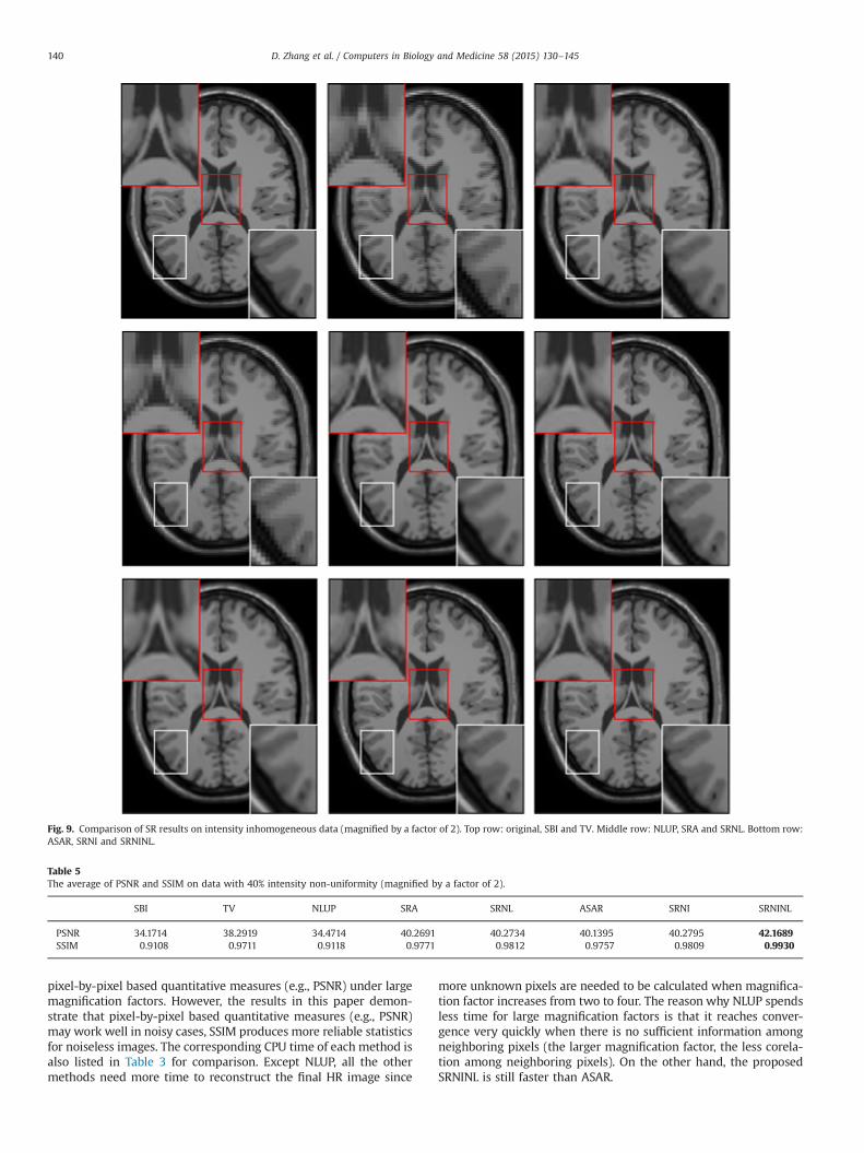
the data with 40% intensity non-uniformity (0% noise) and repeatthe same procedure as we did in the previous two experiments.Fig. 9 presents the reconstructed results of the same slice in Fig. 7by all the tested methods and Table 5 lists the correspondingquantitative measures. By comparing Fig. 9 with Fig. 7, as well asTable 5 with Table 2, we can easily see that

1) Intensity non-uniformity makes almost invisible structurechanges to the original clean slice.

2) The performance of SBI, TV, SRA, SRNL, ASAR, SRNI and SRNINL arealmost the same as they are in Section 6.3.1, since they all build a2D HR image from the given 2D LR image. Moreover, SRNINL stillproduces the best result among all the tested methods.

3) The performance of NLUP degrades dramatically in Fig. 9 andTable 5. This is mainly because that though intensity non-uniformity does not make great visible structure changes insideslice plane, it causes interslice structure changes, which willhamper NLUP to extract useful sub-pixel information viainterslice correspondence.

6.3.4. SR results under large magnification factorIn the previous experiments, the scaling factor is fixed to 2.

However, it could be interesting to test the algorithms’ performanceunder a larger magnification factor, since more HR patch patternsare associated to a single LR patch. To this end, we set the scalingfactor to 4, with a patch size of 3�3 in LR image and 12�12 in HRimage. For SRNL, SRNINL, and SRA, we do not use the LR imagesdownsampled by a factor of 4 to construct a new dictionary Ψl

as Rueda et al. did in [21], we instead adopt the same dictionaries


Fig. 6. Illusion of the performance of SRNINL (in PSNR) over the variation of λ; η, σN ; σR ; α; and X.


Fig. 7. Comparison of SR results (magnified by a factor of 2). Top row: original, SBI and TV. Middle row: NLUP, SRA and SRNL. Bottom row: ASAR, SRNI and SRNINL. (Forinterpretation of the references to color in this figure legend, the reader is referred to the web version of this article.)

Table 2The average of PSNR and SSIM on clean data (magnified by a factor of 2).

SBI TV NLUP SRA SRNL ASAR SRNI SRNINL

PSNR 33.918 37.496 41.292 39.559 40.144 39.454 39.363 43.033SSIM 0.9088 0.9702 0.9862 0.9774 0.9833 0.9766 0.9802 0.9952

Table 3The average of CPU time on clean data (seconds).


CPU time �2 0.003 5.726 1.106 107.371 104.974 138.945 4.904 107.805�4 0.004 133.967 0.519 145.578 123.318 150.782 15.478 134.209


used in the previous experiments and magnify a LR image by twoconsecutive steps with a magnification of 2 for each step. For TV,NLUP, ASAR, and SRNI, we simply magnify the LR image by a factorof 4 since the codes provided by the authors are capable ofexecuting a magnification of 4 directly. Fig. 10 presents one of thereconstructed slices by all the methods and the correspondingnumeric results are reported in Table 6. From Fig. 10, we can still

see that the proposed SRNINL algorithm produces the best resultamong all the tested algorithms. However, Table 6 shows that thePSNR of SRNINL is lower than that of SRNL, though it generatesvisually more appealing image than SRNL does. This is because forthe proposed SRNINL algorithm, an extra post-filtering operation (ifwe add Algorithm 1, the sparse derivative prior based post-filteringoperation into SRNL, it turns out to be SRNINL) may degrade

Fig. 8. Comparison of SR results on noisy data (magnified by a factor of 2). Top row: original, SBI and TV. Middle row: NLUP, SRA and SRNL. Bottom row: ASAR, SRNI andSRNINL. (For interpretation of the references to color in this figure legend, the reader is referred to the web version of this article.)

Table 4The average of PSNR and SSIM on data with 9% noise (magnified by a factor of 2).


PSNR 30.205 30.694 30.841 30.895 30.881 30.847 30.944 32.281SSIM 0.6883 0.7124 0.7529 0.6831 0.7438 0.7503 0.6862 0.7455


pixel-by-pixel based quantitative measures (e.g., PSNR) under largemagnification factors. However, the results in this paper demon-strate that pixel-by-pixel based quantitative measures (e.g., PSNR)may work well in noisy cases, SSIM produces more reliable statisticsfor noiseless images. The corresponding CPU time of each method isalso listed in Table 3 for comparison. Except NLUP, all the othermethods need more time to reconstruct the final HR image since

more unknown pixels are needed to be calculated when magnifica-tion factor increases from two to four. The reason why NLUP spendsless time for large magnification factors is that it reaches conver-gence very quickly when there is no sufficient information amongneighboring pixels (the larger magnification factor, the less corela-tion among neighboring pixels). On the other hand, the proposedSRNINL is still faster than ASAR.

Fig. 9. Comparison of SR results on intensity inhomogeneous data (magnified by a factor of 2). Top row: original, SBI and TV. Middle row: NLUP, SRA and SRNL. Bottom row:ASAR, SRNI and SRNINL.

Table 5The average of PSNR and SSIM on data with 40% intensity non-uniformity (magnified by a factor of 2).


PSNR 34.1714 38.2919 34.4714 40.2691 40.2734 40.1395 40.2795 42.1689SSIM 0.9108 0.9711 0.9118 0.9771 0.9812 0.9757 0.9809 0.9930


6.4. Tests on ADNI dataset

The data used in this section were obtained from the Alzheimer’sDisease Neuroimaging Initiative (ADNI) database [45]. The PrincipalInvestigator of ADNI is Michael W.Weiner, MD, VAMedical Center andUniversity of California. ADNI is the result of efforts of manycoinvestigators from a broad range of academic institutions and

private corporations. The primary goal of ADNI has been to testwhether serial MR imaging, positron emission tomography (PET),other biological markers, and clinical and neuropsychological assess-ment can be combined to measure the progression of mild cognitiveimpairment (MCI) and early Alzheimer’s disease (AD).

We download the data and repeat the same procedure as wedid in the previous experiments. Fig. 11 presents one of the

Fig. 10. Comparison of SR results (magnified by a factor of 4). Top row: original, SBI and TV. Middle row: NLUP, SRA and SRNL. Bottom row: ASAR, SRNI and SRNINL.

Table 6The average of PSNR and SSIM on clean data (magnified by a factor of 4).


PSNR 31.785 33.170 33.319 33.211 34.110 33.459 33.250 34.079SSIM 0.7182 0.8614 0.8652 0.8581 0.8861 0.8640 0.8565 0.9096


reconstructed slices by all the methods and the correspondingnumeric results are reported in Table 7. From Fig. 11, we can seethat for the down-right area (marked by the red box), SRA andASAR produce the most blurry results. By incorporating thenonlocal similarity information properly, SRNL and NLUP producemore clear tissue structures. Though SRNI produces better resultthan SRNL does, by jointly using sparse representation prior,nonlocal similarity and sparse derivative prior, the proposedSRNINL recovers more fine details. Note that in Table 7 thequantitative measures of NLUP are higher than that of SRNI, whichis in contradiction with the visual perception shown in Fig. 11.

6.5. Tests on Cardiac MRI dataset

The Cardiac MRI dataset [46] contains 4D MR images acquiredfrom 33 subjects. Each subject’s sequence consists of 20 frames and8–15 slices along the long axis, for a total of 7980 images. Since theoriginal data contains time axis, we simply choose the volume data bysetting t to zero and repeat the same procedure as we did in theprevious experiments. Fig. 12 presents one of the reconstructed slicesby all the methods and the corresponding numeric results are

reported in Table 8. From Fig. 12, we can see that for the tissuesmarked by the small white and red boxes, SRA and ASAR still producethe most blurry results. On the other hand, SRNL and NLUP producemore clear tissue structures since nonlocal similarity information isproperly incorporated into the reconstruction process. The resultyielded by SRNI is slightly better than that of SRNL. Nevertheless,our proposed SRNINL still produces the best tissue structures amongall the tested methods. Again, as we found in Table 7, though SRNIgenerates visually more appealing image than NLUP does, in Table 8,the quantitative measures of NLUP are higher than that of SRNI.

7. Discussion

In this paper, we propose a new algorithm for reconstructing aHR image from a single LR MR image by jointly using sparserepresentation prior, nonlocal similarity, and sparse derivativeprior. The proposed method has been demonstrated to achievemuch better results than many state-of-the-art algorithms interms of both quantitative measures and visual perception. Ourmain contribution is threefold: (1) the use of multi-scale first- and

Fig. 11. Comparison of SR results on ADNI dataset (magnified by a factor of 2). Top row: original, SBI and TV. Middle row: NLUP, SRA and SRNL. Bottom row: ASAR, SRNI andSRNINL. (For interpretation of the references to color in this figure legend, the reader is referred to the web version of this article.)


second-order derivative analysis to estimate the missing high-frequency information, (2) the joint use of sparse representationand nonlocal similarity under a unified L1-norm minimizationframework, and (3) the use of sparse derivative prior based post-processing in MR image SR reconstruction.

The use of multi-scale edge analysis to estimate high-frequencyinformation was first proposed by Rueda et al. [21] based on twoconsiderations: (1) compared with low-frequency information,high-frequency information has more influence on the reconstruc-tion of sharp edges, and (2) image coherence and regularity are also

Table 7The average of PSNR and SSIM on ADNI dataset (magnified by a factor of 2).


PSNR 35.6354 35.7876 36.4898 35.6288 35.7580 35.6512 35.8142 37.7246SSIM 0.8929 0.8983 0.9199 0.8860 0.9050 0.8871 0.9056 0.9281

Fig. 12. Comparison of SR results on Cardiac MRI dataset (magnified by a factor of 2). Top row: original, SBI and TV. Middle row: NLUP, SRA and SRNL. Bottom row: ASAR,SRNI and SRNINL. (For interpretation of the references to color in this figure legend, the reader is referred to the web version of this article.)

Table 8The average of PSNR and SSIM on Cardiac MRI dataset (magnified by a factor of 2).


PSNR 37.4095 37.5550 38.4542 37.6537 37.8962 37.7649 37.9704 39.6499SSIM 0.9303 0.9350 0.9528 0.9224 0.9400 0.9230 0.9408 0.9703


preserved via multi-scale analysis to some extent, which makespatch overlapping unnecessary. However, only multi-scale first-order derivative analysis was applied in [21]. Since most edges inimages are often gradual transitions from one intensity to another,using first-order derivative one would usually get a curve withrising gradient magnitude, and then a falling gradient magnitude.Extracting the ideal edge is thus a matter of finding this curve withoptimal gradient. For patch-based SR image reconstruction, how-ever, such curve may pass through many neighboring patches, theexact location of the edges would probably be lost for theseneighboring patches are separately reconstructed. Second-orderderivate, on the other hand, could be used to extract optimal edgelocation by finding where it is zero. We must point out that thoughonly the simplest second-order derivative analysis is used in thispaper, using other more reliable ones, e.g., Laplacian operator, Marr–Hildreth operator, is also possible.

Nonlocal similarity refers to the fact that the patches with similarpatterns can be spatially far from each other, we can collect them inthe whole image and process them simultaneously for variouspurposes, e.g., image denoising [29,35], deblurring [16,34], and SR[12,30]. In this paper, by incorporating the nonlocal similarityregularization into the process of MR image SR reconstruction, wegot better results than only using either nonlocal similarity or sparserepresentation prior. Moreover, thanks for the averaging operationof similar patches across the image, the proposed method is morerobust to noise than TV, SRA and SRNI. Finally, the proposed SRNINLalgorithm handles nonlocal similarity information in pixel domain,how about coding nonlocal similarity via sparse representation andincluding it in the same unified SR image reconstruction framework,this is one of our future research directions.

Though natural image prior has been proven to be effective invarious natural image processing tasks, in this paper, we validatethat it is also applicable to MR image processing. In fact, we cansee that a MR image consists mainly of zero gradient regionsinterspersed with occasional strong gradient transitions. By com-paring the results yielded by SRNL and SRNINL, it is easy to findthat a sharp edge is preferred over a blurry one in the final outputwhen applying the natural image prior based post-processingoperation. However, a more direct and elegant approach for jointlyusing sparse representation prior, nonlocal similarity, and sparsederivative prior is to incorporate a sparse derivative prior basedregularization term into (19) as follows

α¼ arg minα

‖yn�ΓΨlα‖22þλ‖α‖1þζ DnΨlα =σ� αn o

ð29Þ

where D is the desired localized, oriented, and bandpass filter, andζ is a parameter controlling the contribution of sparse derivativeprior. Unfortunately, for sparse derivative prior, the exponentparameter α must satisfy 0oαo1, which makes solving (29) viadirectly applying standard L1-norm optimization techniquesimpossible. One of our future research directions will focus onfinding an efficient algorithm to solve (29).

Conflict of interest statement

None declared.

Acknowledgement

This work was supported by the China Postdoctoral ScienceFoundation (Grant no. 2012M511804) and the Natural ScienceFoundation of Guangdong Medical College (Grant no. XB1349).The authors would also like to thank all of the anonymousreviewers for their valuable comments and constructive

suggestions that have significantly improved the presentation ofthis paper.

References

[1] H. Greenspan, Super-resolution in medical imaging, Comput. J. 52 (1) (2008)43–63.

[2] X.G. Wang, X. Tang, Hallucinating face by eigentransformation., IEEE Trans.Syst. Man Cybern. Part C 35 (3) (2005) 425–434.

[3] D. Zhang, H.F. Li, M.H. Du, Fast MAP-based multiframe super-resolution imagereconstruction, Image Vision Comput. 23 (7) (2005) 671–679.

[4] S.C. Park, M.K. Park, M.G. Kang, Super-resolution image reconstruction: atechnical overview, IEEE Signal Process. Mag. (May, 21–36, 2003).

[5] A. Herment, E. Roullot, I. Bloch, O. Jolivet, A.D. Cesare, F. Frouin, J. Bittoun,E. Mousseaux, Local reconstruction of stenosed sections of artery usingmultiple MRA acquisitions, Magn. Reson. Imaging 49 (4) (2003) 731–742.

[6] R. Shilling, T. Robbie, T. Bailloeul, K. Mewes, R. Mersereau, M. Brummer,A super-resolution framework for 3-D high-resolution and high-contrast imagingusing 2-D multislice MRI, IEEE Trans. Med. Imaging 28 (5) (2009) 633–644.

[7] H. Greenspan, G. Oz, N. Kiryati, S. Peled, MRI inter-slice reconstruction usingsuper-resolution, Magn. Reson. Imaging 20 (5) (2002) 437–446.

[8] R. Islam, A.J. Lambert, M.R. Pickering, Super resolution of 3D MRI images usinga Gaussian scale mixture model constraint, in: Proc. ICASSP, 2012, pp. 849-852.

[9] S. Baker, T. Kanade, Limits on super- resolution and how to break them, IEEETrans. Pattern Anal. Mach. Intell. 24 (9) (2002) 1167–1183.

[10] D. Zhang, J.Z. He, M.H. Du, Morphable model space based face super-resolutionreconstruction and recognition, Image Vision Comput. 30 (2) (2012) 100–108.

[11] F. Rousseau. Brain hallucination, in: Proc. the European Conference onComputer Vision: Part I, 2008, pp. 497–508.

[12] J.V. Manjón, P. Coupé, A. Buades, V. Fonov, D.L. Collins, M. Robles, Non-localMRI upsampling, Med. Image Anal. 14 (12) (2010) 784–792.

[13] E. Candès, T. Tao, Near optimal signal recovery from random projections:universal encoding strategies? IEEE Trans. Inf. Theory 52 (12) (2006)5406–5425.

[14] W. Dong, L. Zhang, G. Shi, X. Li, Nonlocally centralized sparse representationfor image restoration, IEEE Trans. Image Process 22 (4) (2013) 1620–1630.

[15] J. Yang, J. Wright, T. Huang, Y. Ma, Image super-resolution via sparserepresentation, IEEE Trans. Image Process 19 (11) (2010) 2861–2873.

[16] W. Dong, L. Zhang, G. Shi, X. Wu, Image deblurring and super-resolution byadaptive sparse domain selection and adaptive regularization, IEEE Trans.Image Process 20 (7) (2011) 1838–1857.

[17] L. Michael, L.D. David, J.M. Santos, M.P. John, Compressed sensing MRI, IEEESignal Process. Mag. 25 (2) (2008) 72–82.

[18] J.C. Ye, S. Tak, Y. Han, H.W. Park, Projection reconstruction MR imaging usingFOCUSS, Magn. Reson. Med. 57 (4) (2007) 764–775.

[19] G. Adluru, C. McGann, P. Speier, E.G. Kholmovski, A. Shaaban, E.V.R. DiBella,Acquisition and reconstruction of undersampled radial data for myocardialperfusion magnetic resonance imaging, J. Magn. Reson. Imaging 29 (2) (2009)466–473.

[20] S. Ravishankar, Y. Bresler, MR image reconstruction from highly undersampledk-space data by dictionary learning, IEEE Trans. Med. Imaging 30 (5) (2011)1028–1041.

[21] Andrea Rueda, Norberto Malpica, Eduardo Romero, Single-image super-resolution of brain MR images using overcomplete dictionaries, Med. ImageAnal. 17 (1) (2013) 113–132.

[22] D. Zhang, M.H. Du Super-resolution image reconstruction via adaptive sparserepresentation and joint dictionary training, in: Proc. CISP, 2013, pp. 492-497.

[23] L. Rudin, S. Osher, E. Fatemi, Nonlinear total variation based noise removalalgorithms, Phys. D 60 (1992) 259–268.

[24] S.D. Babacan, R. Molina, A.K. Katsaggelos. Total variation super resolution usinga variational approach, in: Proc. Int. Conf. Image Process, 2008, pp. 641–644.

[25] H.A. Aly, E. Dubois, Image up-sampling using total-variation regularizationwith a new observation model, IEEE Trans. Image Process 14 (10) (2005)1647–1659.

[26] A. Marquina, S.J. Osher, Image super-resolution by TV-regularization andBregman iteration, J. Sci. Comput. 37 (2008) 367–382.

[27] J. Wright, A.Y. Yang, A. Ganesh, S.S. Sastry, Y. Ma, Robust face recognition viasparse representation, IEEE Trans. Pattern Anal. Mach. Intell. 31 (2) (2009)210–227.

[28] R. Tibshirani, Regression shrinkage and selection via the lasso, J. R. Stat. Soc.,Ser. B 58 (1) (1994) 267–288.

[29] L. Zhang, W. Dong, D. Zhang, G. Shi, Two-stage image denoising by principalcomponent analysis with local pixel grouping, Pattern Recognit. 43 (4) (2010)1531–1549.

[30] M. Protter, M. Elad, H. Takeda, P. Milanfar, Generalizing the nonlocal means tosuper-resolution reconstruction, IEEE Trans. Image Process 18 (1) (2009) 36–51.

[31] ⟨http://sparselab.stanford.edu/⟩.[32] Z. Wang, A.C. Bovik, H.R. Sheikh, E.P. imoncelli, Image quality assessment:

from error visibility to structural similarity, IEEE Trans. Image Process 13 (4)(2004) 600–612.

[33] D.L. Collins, A.P. Zijdenbos, V. Kollokian, J.G. Sled, N.J. Kabani, C.J. HolmesA.C. Evans, Design and construction of a realistic digital brain phantom, IEEETrans. Med. Imaging 17 (3) (1998) 463–468.


http://refhub.elsevier.com/S0010-4825(15)00002-5/sbref1































































http://sparselab.stanford.edu/







[34] S. Kindermann, S. Osher, P.W. Jones., Deblurring and denoising of images bynonlocal functional, Multiscale Model. Simul. 4 (4) (2005) 1091–1115.

[35] A. Buades, B. Coll, J.M. Morel., A review of image denoising algorithms, with anew one, Multiscale Model. Simul. 4 (2) (2005) 490–530.

[36] I.K. Kwang, K. Younghee, Single-image super-resolution using sparse regres-sion and natural image prior, IEEE Trans. Pattern Anal. Mach. Intell. 32 (6)(2010) 1127–1133.

[37] M.F. Tappen, B.C. Russel, W.T. Freeman. Exploiting the sparse derivative priorfor super-resolution and image demosaicing, in: Proc. IEEE Workshop Statis-tical and Computational Theories of Vision, 2003.

[38] B.A. Olshausen, D.J. Field, Emergence of simple-cell receptive field propertiesby learning a sparse code for natural images, Nature 381 (1996) 607–609.

[39] D.L. Ruderman, W. Bialek, Statistics of natural images: scaling in the woods,Phys. Rev. Lett. 73 (6) (1994) 814–817.

[40] E.P. Simoncelli. Statistical models for images: compression, restoration andsynthesis, in: 31st Asilomar Conference on Signals Systems, and Computers.Pacific Grove, CA, 1997, pp. 673–678.

[41] E.P. Simoncelli, Bayesian denoising of visual images in the wavelet domain,Lecture Notes in Statistics, vol. 141, Springer-Verlag, New York (1999) 291–308.

[42] R.W. Buccigrossi, E.P. Simoncelli, Image compression via joint statisticalcharacterization in the wavelet domain, IEEE Trans. Image Process 8 (12)(1999) 1688–1701.

[43] J. Dias. Fast GEM wavelet-based image deconvolution algorithm, in: IEEEInternational Conference on Image Processing, 2003.

[44] M. Figueiredo, R. Nowak Image restoration using the EM algorithm andwavelet-based complexity regularization, in: International Conference onImage Processing, 2002.

[45] ⟨http://adni.loni.usc.edu/⟩.[46] A. Alexande, K.T. John, Efficient and generalizable statistical models of shape

and appearance for analysis of Cardiac MRI, Med. Image Anal. 12 (3) (2008)335–357.

[47] J. Yang, A.F. Frangi, J.Y. Yang, D. Zhang, J. Zhong, KPCA plus LDA: a completekernel fisher discriminant framework for feature extraction and recognition,IEEE Trans. Pattern Anal. Mach. Intell. 27 (2) (2005) 230–244.

[48] M. Irani, S. Peleg, Motion analysis for image enhancement: resolution,occlusion, and transparency, J. Visual Commun. Image Represent. 4 (4)(1993) 324–335.

[49] D. Capel, Image Mosaicing and Super-Resolution, Springer-Verlag, 2004.

Di Zhang received his M.Sc. in Physics in 1996 from Wuhan University, Wuhan,China, and his Ph.D. in Communication and Information Systems in 2005 fromSouth China University of Technology, Guangzhou. From 2005 to 2011, He joinedthe Department of Computer Science, Shaoguan University, Shaoguan. He iscurrently an Associate Professor at the School of Information Engineering, Guang-dong Medical College, Dongguan. His current research interests include signalprocessing, image processing and pattern recognition.

Jiazhong He received his Ph.D. degree in communication and information systemsin 2007 from South China University of Technology, Guangzhou. He is currently anassociate professor at the Department of Physics, Shaoguan University, Shaoguan.His current research interests include pattern recognition and image processing.

Yun Zhao is currently a teacher at the School of Information Engineering,Guangdong Medical College, Dongguan. Her current research interests includecomputer vision and computer programming.

Minghui Du received his B.Sc. degree in electronics in 1985 from Fudan University,Shanghai, China, and his Ph.D. degree in electronic and communication systems in1991 from South China University of Technology, Guangzhou, where he is currentlya professor with the department of Electronics and communication engineering.Prof. Du is the vice chairman of Guangdong Institute of Graphics and Image, acommittee member of the Chinese institute of Graphics and image, a committeemember of the Chinese institute of biomedical engineering. His current researchinterests include digital imaging, medical image processing, signal processing andbiomedical engineering.


















http://adni.loni.usc.edu/











mr image super-resolution reconstruction using sparse representation, nonlocal...

Documents