This article was downloaded by: [University of Toronto Libraries]On: 25 November 2011, At: 12:25Publisher: Taylor & FrancisInforma Ltd Registered in England and Wales Registered Number: 1072954 Registered office: Mortimer House,37-41 Mortimer Street, London W1T 3JH, UK

International Journal of Production ResearchPublication details, including instructions for authors and subscription information:http://www.tandfonline.com/loi/tprs20

Multi-threaded simulated annealing for a bi-objectivemaintenance scheduling problemNima Safaei a , Dragan Banjevic a & Andrew K.S. Jardine aa Department of Mechanical and Industrial Engineering, University of Toronto, Canada

Available online: 13 Jun 2011

To cite this article: Nima Safaei, Dragan Banjevic & Andrew K.S. Jardine (2011): Multi-threaded simulatedannealing for a bi-objective maintenance scheduling problem, International Journal of Production Research,DOI:10.1080/00207543.2011.571444

To link to this article: http://dx.doi.org/10.1080/00207543.2011.571444

PLEASE SCROLL DOWN FOR ARTICLE

Full terms and conditions of use: http://www.tandfonline.com/page/terms-and-conditions

This article may be used for research, teaching, and private study purposes. Any substantial or systematicreproduction, redistribution, reselling, loan, sub-licensing, systematic supply, or distribution in any form toanyone is expressly forbidden.

The publisher does not give any warranty express or implied or make any representation that the contentswill be complete or accurate or up to date. The accuracy of any instructions, formulae, and drug doses shouldbe independently verified with primary sources. The publisher shall not be liable for any loss, actions, claims,proceedings, demand, or costs or damages whatsoever or howsoever caused arising directly or indirectly inconnection with or arising out of the use of this material.

International Journal of Production Research2011, 1–18, iFirst

Multi-threaded simulated annealing for a bi-objective maintenance scheduling problem

Nima Safaei*, Dragan Banjevic and Andrew K.S. Jardine

Department of Mechanical and Industrial Engineering, University of Toronto, Canada

(Final version received February 2011)

A parallel Simulated Annealing algorithm with multi-threaded architecture is proposed to solve a real bi-objective maintenance scheduling problem with conflicting objectives: the minimisation of the total equipmentdowntime caused by maintenance jobs and the minimisation of the multi-skilled workforce requirements overthe given horizon. The maintenance jobs have different priorities with some precedence relations betweendifferent skills. The total weighted flow time is used as a scheduling criterion to measure the equipmentavailability. The multi-threaded architecture is used to speed up a multi-objective Simulated Annealingalgorithm to solve the considered problem. Multi-threading is a form of parallelism based on shared memoryarchitecture where multiple logical processing units, so-called threads, run concurrently and communicate viashared memory. The performance of the parallel method compared to the exact method is verified using anumber of test problems. The obtained results imply the high efficiency and robustness of the proposedheuristic for both solution quality and computational effort.

Keywords: maintenance scheduling; workforce allocation; multi-objective optimisation; mixed-integerprogramming; parallel simulated annealing; multi-threading

1. Introduction

Today, maintenance service is an essential sector of industry with the aim of increasing the reliability and availabilityof production equipment to meet growing competition in the global market. This sector is responsible for decreasingthe downtime of equipment through both preventive maintenance (PM) actions and timely responses to occasionalrequests upon unexpected or potential failures. However, improved efficiency of maintenance service requires bettermanagement of the available resources among the skilled workforce. Hence, the scheduling of the PM and failurerepair (FR) jobs is an important issue for a maintenance department. The occurrence time of failures is almostunpredictable, and jobs have different priorities and degrees of importance. Moreover, maintenance jobs are labourintensive, and the workforce performing these jobs is often highly paid and highly skilled with differentproficiencies. This means job scheduling should minimise the workforce costs, and a trade-off must be madebetween workforce cost and the timely completion of all maintenance jobs by the maintenance department.

The key contribution of this article is to provide an efficient approach to solving a real maintenance schedulingproblem already investigated in a recently published paper by the authors (Safaei et al. 2011). The consideredproblem is related to a steel company which has recently moved to a plant-wide scheduling approach through acentral department, called Central Services Department (CSD), which responds to the maintenance requirements ofmanufacturing areas (MAs) located in the plant. The aim of this department is to minimise the workforce costs aswell as to avoid long-term disruptions and equipment shutdown within MAs. Note that there is no correlationamong the failures and all equipment breakdowns are independent. Each MA schedules its maintenance jobs andsubmits them to CSD which, in turn, attempts to schedule the skilled workforce to meet needs across the plant.Given the number and variety of jobs, the limitation of labour resources and job priorities, CSD has foundit difficult to prioritise maintenance jobs and to optimally schedule them while considering the available resources.It is worth noting that maintainers with different skills are categorised into a number of trades with variousproficiencies.

The considered problem is NP-hard in a strong sense because it is a combination of ‘scheduling’ and ‘allocation’problems. In other words, maintenance jobs should be scheduled over the given planning horizon, while theworkforce volume required per period of horizon cannot exceed the available labour resource. Moreover, as pointed

*Corresponding author. Email: safaei@mie.utoronto.ca

ISSN 0020–7543 print/ISSN 1366–588X online

� 2011 Taylor & Francis

DOI: 10.1080/00207543.2011.571444

http://www.informaworld.com

Dow

nloa

ded

by [

Uni

vers

ity o

f T

oron

to L

ibra

ries

] at

12:

25 2

5 N

ovem

ber

2011

out earlier, because we encounter a multi-skilled workforce, jobs should be scheduled in different trades in a parallel

manner. Considering each period of the horizon as a ‘knapsack’, we solve the ‘parallel scheduling’ and ‘multiple

knapsack’ problems concurrently. Furthermore, because of uncertainty over the workforce availability, CSD would

like to have alternative solutions/schedules for different workforce sizes. These alternative solutions provide some

flexibility, thus ensuring better decision making. They also help CSD achieve a compromise solution for external/

subcontracted resource planning. A further complication is that a proportion of the available labour is usually

reserved for catastrophic failures or emergency situations. To avoid the repetitious solving of a single-objective

problem and to simultaneously provide alternative solutions, we have selected the multi-objective strategy

(Quan et al. 2007). That is, the minimisation of the workforce requirements is considered an objective function.

On the other hand, because of the stochastic nature of equipment failure, we have a dynamic environment in which

jobs are re-scheduled frequently over a short term horizon, say a day. With all these complexities, it is difficult to

solve the considered problem using traditional optimisation approaches in a reasonable time.With the increasing computational ability of computers, stochastic search-based and meta-heuristic approaches

are becoming a reality in the combinatorial optimisation field. In practice, many of these novel approaches fail to

reach near optimal solutions within an acceptable time, especially when we encounter the so-called ‘combinatorial

explosion’ for overly complex problems. In short, these approaches should somehow be speeded up. One way to

speed up meta-heuristics is to use parallel or distributed approaches. The rapid evolution of technology in computer

science in terms of processors, networks and architectures makes parallelisation very popular. From an optimisation

point of view, a parallel strategy can be defined as simultaneously searching different regions of the solution/

objective space with two or more processing units with the aim of increasing the search efficiency and decreasing the

CPU time. There may be some interaction between the processing units as they interchange elite solutions or

synchronise information; such interactions are necessary to avoid interference in the processing of the units.

Different architectures are available to develop parallel applications, including message passing, shared memory,

high throughput computing, and grid computing (Talbi et al. 2008). The parallel processing units are the physical

units integrated in a single computer or distributed in a network (Master–Slave structure) or they are logical units

run simultaneously on a single processor. Multi-threading is a form of parallelism based on shared memory

architecture where multiple logical processing units, so-called threads, run concurrently and communicate via

shared memory. In this strategy, the processor switches between different threads. This context switching can

happen so fast as to give the illusion of simultaneity to the end user. Actually, threads are a way for a program to

fork (or split) itself into two or more pseudo-simultaneously running tasks. From an algorithmic point of view,

multi-threading is used to enlarge the available amount of concurrently executable instructions by providing access

to more than a single independent instruction stream. Larger or smaller independent sequences of instructions

(threads) can be found in nearly all algorithms (Wittenburg et al. 1999), including meta-heuristic algorithms. The

main advantages of multi-threading over other parallel architectures are lower hardware requirements, lower

specialist knowledge, and flexibility in the number of used threads. With present technologies, the user can employ

up to 25 threads simultaneously on a single processor.In this article, we propose Multi-Threaded Simulated Annealing (MTSA) to solve the considered problem; here,

two threads operate simultaneously, each responsible for searching a certain region of the objective space. The

proposed MTSA supposes that the optimal Pareto set (OPS) is a bi-section curve, and each section is constructed by

a thread. Each thread has its own Pareto archive, and there is no interaction between threads. Moreover, in the

proposed MTSA, the archived Pareto solutions and their neighbours can be combined to generate new solutions, a

mechanism which helps the threads remain in their assigned regions as much as possible. The above features

constitute the advantages of the proposed approach; because of them, CPU time is significantly decreased while the

size of the common region being searched by both threads is significantly reduced. This results in high efficiency and

a robust search process. It is worth noting that communication between threads is an inherent drawback of multi-

threading because it results in low efficiency and race conditions between threads for access to shared memory (Evjen

et al. 2008). Finally, to the best of our knowledge, none of the approaches proposed in the literature guarantees that

the threads will remain in their assigned regions (Talbi et al. 2008). Hence, there will always be a common search

region between the threads.The rest of this article is organised as follows. Section 2 gives a literature review of the workforce-constrained

maintenance scheduling and parallel approaches for optimisation. Section 3 describes the problem and presents its

formulation. The implementation of the proposed MTSA is explained in Section 4, and its performance is verified

and discussed in Section 5. Section 6 constitutes a conclusion and provides suggestions for future research.

2 N. Safaei et al.

Dow

nloa

ded

by [

Uni

vers

ity o

f T

oron

to L

ibra

ries

] at

12:

25 2

5 N

ovem

ber

2011

2. Literature review

Whilst the literature on maintenance scheduling problem is intensive, only a few studies focus on the workforce as amajor concern. A comprehensive review of the literature on workforce-constrained maintenance scheduling problemcan be found in Safaei et al. (2011). Wagner et al. (1964) were the first to formulate the PM job-scheduling problemas a mathematical programming model with the aim of minimising/balancing the fluctuation of workforcerequirements during a given horizon. Subsequent studies considered the workforce factor with different assumptionsand objectives, including optimal workforce size determination (Vergin 1966), workforce utilisation maximisation(Roberts and Escudero 1983, Mjema 2002), multi-skilled workforce availability (Gopalakrishan et al. 1997, Higgins1998, Ahire et al. 2000), subcontracting (Yanga et al. 2003), and workforce cost minimisation (Quan et al. 2007).

A number of studies have taken novel approaches to solving maintenance scheduling problems. For instance,Quere et al. (2003) proposed a reactive scheduling approach to schedule the maintenance jobs in a system with a set ofhighly-specialised and resource-independent decision centres that must be coordinated to ensure global performance.However, each centre has its own objective which could be dependent or contradictory with others. Safaei et al. (2008)solved a workforce-constrained maintenance scheduling problem using a multi-objective simulated annealingalgorithm. Marmier et al. (2009) proposed a dynamic scheduling approach to schedule maintenance jobs byconsidering the insertion of new jobs into a current schedule. They assumed the submission date and due date of PMjobs to be uncertain; the processing time of FR jobs was also assumed to be uncertain. Maintainers were considered ashaving different proficiencies with uncertain qualification levels and uneven competency rates. The total weightedtardiness was used as a measure of asset availability. In their solution, the weight of each job represents its priority andis determined by the penalty which could be claimed if the job were not completed on time.

The literature on parallel approaches to optimisation problems is relatively strong; however, it is rare to findpreviouswork focusing onmulti-threaded architecture formeta-heuristics. A comprehensive taxonomy of parallel anddistributed approaches for multi-objective optimisation can be found in Talbi et al. (2008). In the area of parallel anddistributed architectures for SA, Sohn (1995) used a parallel strategy called Generalised Speculative Computation(GSC) to solve TSPwith amaximumof 500 nodes.GSCuses an n-ary speculative tree to execute ndifferent iterations inparallel on nprocessors.ApplyingGSC toSA, he obtained anover 20-fold speedupon100processors.Ram et al. (1996)proposed two distributed SA algorithms and applied these to the job shop scheduling problem and TSP. Theyimplemented the proposed algorithms in a network of 18 SUNworkstations and obtained satisfactory results. In theirsolutions, each network node runs an SA algorithm using a different initial solution. After a fixed number of iterations,the nodes exchange the partial results to get the best one. With respect to multi-threaded meta-heuristics, Zalzala andGreen (1999) proposed a multi-threaded genetic programming (MTGP) application that has since been developed byJava applets. In MTGP, the individuals from four sub-populations are manipulated concurrently, and these sub-populations exchange their best individuals at fixed intervals during a run. Each sub-population is handled by a thread.Finally, Lazarova (2008) investigated the efficiency of MTSA and a distributed SA to solve a room assignmentproblem. In the proposed MTSA, each thread constructs and manipulates a portion of the current solution.

3. Problem description

3.1 Nomenclature

T length of the planning horizon in terms of a given unit time (say hour)M number of maintenance jobs submitted to CSDK number of tradesrm submission time of job mdm due date of job m

ptmk processing time required for trade k to do job mWmk required number of maintainers of trade k to do job m

pmkl¼ 1 if trade k must be completed immediately before trade l (precedence relations) on job m; and equals zerootherwise

wm weigh or priority of job mstmk starting time of job m by trade kctmk completion time of job m by trade k’m overall completion time of job m where ’m¼maxk{ctmk}�k size of trade k

International Journal of Production Research 3

Dow

nloa

ded

by [

Uni

vers

ity o

f T

oron

to L

ibra

ries

] at

12:

25 2

5 N

ovem

ber

2011

At the beginning of the time horizon (zero time), M jobs consisting of preventive and corrective/repairmaintenance tasks have been already submitted to CSD and should be scheduled over the incoming horizon. Eachjob m has been submitted rm unit times before zero time (�rm� 0) and must be finished by the given due date dim� 0.Note that dm may or may not be greater than the horizon length T. Moreover, each job m has a priority that isspecified by weight wm so that wm(0, 1) and

Pmwm¼ 1. The priority of the jobs is determined by the local crew in

MAs based on such criteria as equipment downtime criticality, equipment maintainability, and severity of the failure(Moore and Starr 2006). In general, the jobs causing high downtime for equipment also have a high priority inscheduling. Jobs associated with critical or bottleneck equipment also have relatively high priority (Gopalakrishanet al. 1997). Sometimes jobs may be prioritised based on the customer orders awaiting the repair of failed equipment(Worrall and Mert 1989). In our case, the due date has a direct relationship on job priority. That is, the higher thejob priority, the earlier its due date. Obviously, jobs with due dates during the new horizon should be considered ashaving the highest priority (Gopalakrishnan et al. 1997). Without loss of generality, assuming insufficient resources,jobs with late due dates or low priority can be postponed for scheduling in succeeding periods.

As pointed out earlier, skilled maintainers are divided into a number of trades with specific proficiencies, such asmechanical, electrical, pipefitting and lubrication. Each job needs the input of more than one trade to be completed.The required number of maintainers of trade k to carry out job m (Wmk) as well as the time required to process(ptmk) can be estimated using the CMMS1 dataset and expert knowledge. Precedence relations between the tradesmust also be considered.

The main objective is to minimise the total equipment downtime caused by maintenance jobs. From a schedulingpoint of view, the downtime of equipment is equivalent to the flow time of the corresponding maintenance job. Theflow time is defined as the difference between the submission and the completion times of a job; during this period, theequipment will obviously not be available. It is assumed that the equipment has been stopped at the time of submissionwith the aim of preparing it for PM/repair tasks or preventing possible secondary failures. Because jobs have differentpriorities, the minimisation of the total weighted flow time (TWFT) is considered an objective. TWFT can be stated asPM

m¼1 wmðctm � rmÞwhere ctm represents the completion time of jobm. TWFTminimisation ensures that high-priorityjobs are scheduled before low-priority jobs. However, concentrating only on this objective increases the workforcerequirement, defined as the number of required maintainers of all trades to do all jobs over the time horizon.Moreover, as discussed earlier, CSD is interested in alternative solutions/schedules in terms of workforce size. Hence,the minimisation of workforce requirements is the second objective. The trade-off between these two conflictingobjectives results in a set of non-dominated Pareto solutions which help CSD make better decisions about theworkforce reserved for emergency situations and even the size of the subcontracted workforce.

The above problem can be considered a parallel scheduling problem in which the various trades can be treated asparallel processors/machines for which maintenance jobs should be scheduled. Each maintenance job represents aproduct with a number of operations that must be done by predetermined trades according to certain precedencerelations. The time-capacity (i.e. available man-hours) of trades is limited over the given horizon. At the beginningof the horizon, the jobs on the waiting list (not yet started) are prioritised along with newly arrived jobs; those withhigher priority are scheduled in the new horizon, depending on the available workforce. It is assumed that thehorizon is long enough to accommodate the estimated duration of the jobs. Otherwise, jobs that have alreadyviolated the horizon length must be considered fixed jobs in the horizon and cannot be re-scheduled. On the otherhand, it is assumed that the horizon is short enough so that the failures which occurred at the middle of the horizoncan be postponed to be scheduled at the next horizon.

A schematic mapping of the considered problem into the parallel scheduling problem with three trades and fivejobs over a daily horizon is shown in Figure 1. Symbol ‘Wm’ represents job m, and bolded rectangles represent theschedule bars corresponding to the jobs. The numbers within the rectangles represent the required number ofmaintainers from the given trades to process the jobs. The length of the rectangles indicates the duration of the jobs.For instance, consider the processing route of W4 in Figure 3. As is evident in the figure, W4 needs Trades 1, 2 and 3to be completed. We assume that Trade 1 must finish the processing of job 4 before Trade 3; this indicates aprecedence relation between Trades 1 and 3 to do W4. Moreover, Trades 1, 2 and 3 need 1, 2 and 1 maintainers and6, 3 and 2 h, respectively, to do W4. If we assume that CSD schedules the jobs every day starting at 8:00 am, then8:00 am represents the scheduling moment (i.e. t¼ 0) used to express the submission time and due date of the jobs.For example, job W4 is submitted 2 h before zero time (i.e. 6:00 am), i.e. r4¼�2, and its due date is 9 h after zerotime (i.e. 3:00 pm), i.e. d4¼ 9. Since job 4 will be completed at t¼ 8, its flow time is 8� (�2)¼ 10 h.

One major concern is the workforce availability limitation. That is, the number of required maintainers of tradek per period t, �tk, cannot exceed the available number of maintainers in trade k over the horizon, �k, whilst the value

4 N. Safaei et al.

Dow

nloa

ded

by [

Uni

vers

ity o

f T

oron

to L

ibra

ries

] at

12:

25 2

5 N

ovem

ber

2011

of �tk completely depends on the current schedule, andP

k�k actually represents the value of the second objectivefunction in the considered problem. Assume that qtmk equals one if job m is being carried out in time period t(stmk� t5 ctmk) and equals zero otherwise. Then, we have �tk ¼

PMm¼1 q

tmk �Wmk, and consequently,

�k ¼ max1�t�Tf�tkg yields the required size of trade k based on the current schedule. Such a strategy to determine

the required size of trades can be extremely complicated from a mathematical programming point of view because itis time dependent and its complexity increases progressively by decreasing the period length.

An alternative strategy is network flow formulation (Safaei et al. 2011) in which the workforce is considered asflow and jobs as nodes in the network. Maintainers are assigned to jobs from a nominal depot and must go back tothe depot after completing the jobs. No matter how the maintainers are assigned to the jobs and move betweenthem, the output and input flows must be equal. In this case, the number of maintainers required to do all jobs is thesame as the input (or output) flow. A typical example of the assignment of the workforce for four scheduled jobs asa network is shown in Figure 2. The icons within the boxes represent the required number of maintainers to do thecorresponding jobs. As evident in this figure, five maintainers are needed to do all the jobs, which is equal to theinput (or output) of the network.

3.2 Mathematical formulation

In this section, the problem is formulated as a bi-objective mixed-integer programming model. The followingnotation is used to formulate the workforce network flow explained in Figure 2.

xkmn number of maintainers of trade k who should shift to job n after completion of job mykmn ¼ 1 if there is a possibility to shift the maintainers of trade k from job m to job n; otherwise equals zero

emk number of maintainers of trade k dispatched from depot to job mzmk number of maintainers of trade k who go back to depot from job n

W1 3 W2 2

Trade 1 W3 14W

W5 2

W1 2 W2 1

Trade 2 W3 3 W4 1 W5 2

W1 1 W2

Trade 3 W3 2 W4 1 W5 2 Time -4 -3 -2 -1 1 2 3 4 5 6 7 8 9

Calendar 4:00 am

5:00 am

6:00 am

7:00 am

8:00 am

9:00 am

10:00 am

10:00 am

11:00 am

12:00 pm

01:00 pm

02:00 pm

03:00 pm

doireptxeNdoirepsuoiverP

ct4st4d4

r4Flow time

Downtime

Figure 1. Mapping of considered problem into the parallel scheduling problem.

1

2

111

1 2

2

1Input flow Output flow

Depot Depot

Figure 2. Calculation of the Workforce requirements as a network flow problem.

International Journal of Production Research 5

Dow

nloa

ded

by [

Uni

vers

ity o

f T

oron

to L

ibra

ries

] at

12:

25 2

5 N

ovem

ber

2011

Mþ positive large number" positive small number

Using the above notation and the provided nomenclature, the proposed model is stated as

minZ1 ¼XMm¼1

wm ’m � rmð Þ ð1Þ

minZ2 ¼XKk¼1

�k ð2Þ

s.t:

ctmk ¼ stmk þ ptmk 8k,m; ptmk 4 0 ð3Þ

’m � ctmk 8m, k ð4Þ

’m � dm 8m ð5Þ

ctmk � stml � 0 8k, l,m; pmkl ¼ 1, ptmk 4 0, ptml 4 0 ð6Þ

ykmn � 1þ stnk�ctmk

Mþ

� �ykmn � "þ

stnk�ctmk

Mþ

� ��

8m, n, k; ptmk 4 0, ptnk 4 0,m 6¼ n ð7Þ

xkmn �Mþ � ykmn 8m, n, k; ptmk 4 0, ptnk 4 0 ð8Þ

XMm¼1m 6¼n

xkmn þ enr ¼Wmk 8n, k; ptnk 4 0 ð9Þ

XMn¼1n6¼m

xkmn þ smk ¼Wmk 8m, k; ptmk 4 0 ð10Þ

�k ¼XMm¼1

zmk 8k ð11Þ

ykmn 2 f0, 1g, xkmn, emk, zmk, ctmk, stmk, ’m � 0, �k 2 N

þð12Þ

The objective function given in Equation (1) is intended to minimise TWFT. The objective function in Equation

(2) is to minimise the workforce requirements. Equation (3) computes the completion time of the jobs on trades.

Constraint (4) determines the overall completion time of the jobs. Inequality (5) requires that the overall completion

time cannot violate the due date. Constraint (6) guarantees the satisfaction of precedence relations between the

trades. Constraints (7) and (8) are used to compute the required number of maintainers according to the network

flow strategy explained in Figure 2. As noted, there is a nominal depot for each trade, and all maintainers must be

dispatched from and go back to this depot. In Constraint (7), the values ofMþ and " should be determined such that

Mþ4max{stnk� ctmk} and "5min{stnk –ctmk} 8k, m, n and m6¼n. To satisfy these conditions, we assume that

Mþ¼Tþ 1 and "¼ 0.001 represent selected errors so that a¼ b() |a� b|� ". Constraints (7) and (8) ensure that

some maintainers of trade k released from job m may be shifted to job n, if ctmk� stmk. Constraint (9) guarantees

that the total input flow re-assigned to a given job will satisfy the job workforce requirements. Likewise, Constraint

(10) ensures that the total output flow from a given job is equal to its input flow. Constraints (9) and (10) guarantee

that the total input and output flow of the network is equal. Constraint (11) determines the size of each trade to be

6 N. Safaei et al.

Dow

nloa

ded

by [

Uni

vers

ity o

f T

oron

to L

ibra

ries

] at

12:

25 2

5 N

ovem

ber

2011

used in the second objective function. For more details about the proposed model, refer to Safaei et al. (2011).To generate the optimal Pareto set (OPS) for the given problem, the classical "-Constraint algorithm is used asfollows (Miettinen 1999):

fMinimise Z1 subject to the original constraints, Z2 5 " and Zmin2 5 " � Zmax

2 g,

where Zmin2 and Zmax

2 are the minimum and maximum values of the second objective function, respectively. Thesevalues are obtained by solving the proposed model with the individual objective functions using the Branch-and-Bound (B&B) method. At each iteration of the algorithm, the value of " is replaced by the recently obtained value ofZ2, and the model is solved again until no improvement in " is possible. The set of solutions obtained during theiterations forms the OPS.

4. Multi-threaded simulated annealing

In this section, an MTSA algorithm is developed to solve the bi-objective model proposed in Section 3. The MTSAalgorithm consists of two threads, each containing a revised SA algorithm that is responsible for minimising oneobjective while trying to improve the obtained solutions with respect to another objective. To this end, one Paretoarchive is considered for each thread so that the non-dominated solutions obtained during the search are insertedinto this archive. A newly generated solution will be accepted either if its quality is better than the previous solution(i.e. classical acceptance criterion of SA) or if it is eligible to be added to the Pareto archive of the thread. Thismechanism logically divides the objective space into two search regions, each simultaneously explored by a thread asshown in Figure 3. However, a very small common region will be explored by both threads. After finishing theprocess of all threads, the final Pareto set is created by uniting the Pareto archives of both threads. The pseudo-flowchart of the proposed MTSA is shown in Figure 4. The main idea behind the proposed MTSA is that the OPS isa bi-section curve so that each section is constructed by a thread as depicted in Figure 3.

To significantly increase the exploration power of MTSA, especially at initial iterations, it is possible to combinethe newly generated solution with the solutions in the thread’s Pareto archive. The experimental results show thatthis allows us to find more Pareto solutions whilst keeping the thread within the pre-defined search region so thatthe intersection of the Pareto archive of threads remains at the minimum level during the search. This combinationstrategy is performed by some crossover operators. However, the rate of combination decreases with elapsed time.

The biggest advantage of the proposed mechanism is the non-existence of interactions between the threads; thisleads to a significant reduction in CPU time. It is worth noting that the overlap between the search spaces ofdifferent threads should be as small as possible to be able to increase the efficiency of the search process.

4.1 Solution representation

A matrix consisting of K rows (number of trades) and M columns (number of jobs) is used to represent the solutionof the developed mathematical model. Considering the typical solution X¼ [xkm]K�M, the entry xkm is the same

Z1

Z2

Thread 1 search region

Thread 2 search region

Commonregion

Pareto archive 2

Pareto archive 1

Optimal Pareto Set

Figure 3. Proposed multi-threading strategy for bi-objective optimisation.

International Journal of Production Research 7

Dow

nloa

ded

by [

Uni

vers

ity o

f T

oron

to L

ibra

ries

] at

12:

25 2

5 N

ovem

ber

2011

variable as stmk in the model; this indicates the starting time of job m on trade k. Obviously, some entries in thesolution representation are inherently zero or null since all jobs do not need to be performed by all trades.

4.2 Fitness functions

As discussed earlier, each objective function is optimised by an individual thread. Even so, the solutionrepresentation X¼ [xkm] does not guarantee that the precedence relations presented in Constraint (6) are satisfied.Hence, the fitness function for each thread equals the associated objective function plus a penalty term. The penaltyterm is a proportion of the infeasibility degree corresponding to the given solution multiplied by a penaltycoefficient. The infeasibility degree of a solution is defined as the sum of the time-overlaps resulting from theprecedence relations violation. Note that the total infeasibility should be incurred by both fitness functions tobalance both CPU time and the search power of the threads. Otherwise, the probability of the existence of someinfeasible solutions in the final Pareto set greatly increases. The fitness functions that evaluate the given solution Xin threads 1 and 2 are given as

F1ðXÞ ¼XMm¼1

wm maxK

k¼1fxmkg � rm

� �þ ��

XMm¼1

XKk¼1

XKl¼1

maxfpmkl � ðxmk þ ptmk � xmlÞ, 0g ð13Þ

F2ðXÞ ¼XKk¼1

�k þ �ð1� �ÞXMm¼1

XKk¼1

XKl¼1

maxfpmkl � ðxmk þ ptmk � xmlÞ, 0g ð14Þ

where �40 represents the penalty coefficient, and � (05 �5 1) represents the proportion of infeasibility that shouldbe allocated to fitness function F1. Likewise, (1��) is the proportion of infeasibility that should be allocated tofitness function F2. The second term in Equations (13) and (14) calculates the infeasibility of solution X in whichxmkþ ptmk (¼ctmk) equals the completion time of job m in trade k. The term maxkfxmkg(¼’m) in Equation (13)indicates the overall completion time of job m. In Equation (14), �k is computed based on the time-dependentstrategy explained in Section 3 so that �k ¼ max1�t�Tf�

tkg where �

tk ¼

PMm¼1 q

tmk �Wmk and qtmk¼ 1 if stmk� t5 ctmk

and equals zero otherwise.

4.3 Neighbour solution generation

To generate neighbour solutions, three mutation operators with different structures are developed. Given thecurrent solution X¼ [xkm]K�M, the developed mutation operators are as follows:

. Minor mutation (MIM): The entry xij is randomly selected and then reduced or increased by one with equalprobability,(xkm xkm� 1).

Common region

Thread 1 Thread 2

Start parallel processing

Pareto archive 1 Pareto archive 2

End parallel processing

Final Pareto set = Archive 1 ∪ Archive 2

Updating

Figure 4. Proposed MTSA mechanism.

8 N. Safaei et al.

Dow

nloa

ded

by [

Uni

vers

ity o

f T

oron

to L

ibra

ries

] at

12:

25 2

5 N

ovem

ber

2011

. Moderate mutation (MOM): The entry xij, is randomly selected and then reduced or increased by the

following rules, with equal probability:

� xkm xkmþ z� (dm� xkm) where z!U(0, 1) and dm is due date of job m or,� xkm xkm� z� xkm.

. Major mutation (MAM): This is a boundary mutation which moves the selected entry to the one of its

feasible bounds. That is, the entry xkm is uniformly changed to 0 or dm. Note that in the case of z¼ 1, MOM

and MAM will be same.

Three crossover operators are also considered with the aim of combining the current solution with the solutions in

the Pareto archive of threads. Assume that in the current solution X¼ [xkm]K�M, Pareto solution E¼ [ekm]K�M and a

spare solution Y¼ [ykm]K�M are given. The reason for Y is that the crossover operators always generate two

offspring at the same time. Hence, one offspring will be replaced by X while the other will be saved in spare solution

Y to better search the solution space (Figure 6).

. Arithmetic crossover (AC): This operator generates a linear combination of X and E. That is, a uniform

variable �(0,1) is randomly generated and X elements are updated as xmk ¼ �xmk þ ð1� �Þemk and Y

elements are set to ymk ¼ ð1� �Þxmk þ �emk.. Vertical crossover (VC): The cut-point cp is randomly generated within interval (1, K), i.e. vertical direction

of the solution matrix (Tavakkoli-Moghaddam et al. 2005, Batouche et al. 2006), and the elements of X and

Y are changed as follows:

� xkm ¼ ekm; k ¼ 1, . . . , cp, m ¼ 1, . . . ,M� ykm ¼ xkm for k ¼ 1, . . . , cp, m ¼ 1, . . . ,M and ykm ¼ ekm for k ¼ cpþ 1, . . . ,K, m ¼ 1, . . . ,M

. Horizontal crossover (HC): Likewise, the cut-point cp is randomly generated within interval (1, M), and the

elements of X and Y are changed as follows:

� xkm ¼ ekm; k ¼ 1, . . . ,K, m ¼ 1, . . . , cp� ykm ¼ xkm for k ¼ 1, . . . ,K, m ¼ 1, . . . , cp and ykm ¼ ekm for k ¼ 1, . . . ,K, m ¼ cpþ 1, . . . ,M

4.4 Dynamic tuning of operators

One way to control and balance the exploration and exploitation of the meta-heuristic algorithms during the search

is with a time-varying strategy or the dynamic tuning of the operators. That is, the usage rate of operators will be

changed in an efficient manner as time goes on. The experimental results show that having operators with constant

usage rates significantly decreases the exploration power of MTSA and leads to low-quality solutions and an

imperfect Pareto set. To this end, the following time-varying strategy is applied:

. Overall tuning: At the initial iterations, the crossover is applied at a relatively high rate. However, the

overall rate of crossover is gradually decreased while the overall rate of mutation is increased as time goes

on.. Interior mutation tuning: The interior rate of three mutation operators will be changed during the search.

That is, during the initial iterations, MAM is applied at a high rate and then its power is gradually replaced

by MIM. However, MOM is applied with a constant but moderate rate during the search.. Interior crossover tuning: The three crossover operators AC, VC and HC are applied at the same rate during

the search.

To implement the above strategy, the rate of operators is controlled by the following linear relations:

RuðnÞ ¼ RIu þ

RFu � RI

u

N� 1

� �� ðn� 1Þ; u ¼ 1, 2, 3 ð15Þ

International Journal of Production Research 9

Dow

nloa

ded

by [

Uni

vers

ity o

f T

oron

to L

ibra

ries

] at

12:

25 2

5 N

ovem

ber

2011

rðnÞ ¼ rI þrF � rI

N� 1

� �� ðn� 1Þ ð16Þ

where

Ru(n) rate of mutation type of u at iteration nRI

u initial rate of mutation type of u where u¼ 1, 2 and 3, respectively, represents operators MIM, MOM andMAM

RFu final rate of mutation type of u when algorithm is terminated

r(n) rate of crossover at iteration nrI initial rate of crossoverrF final rate of crossover

Note that Equation (15) ensures R1(n)þR2(n)þR3(n)¼ 1 8n. The integration of the above time-varying strategyinto the neighbour solution generation procedure is shown in Figure 5. This procedure receives current solution X,spare solution Y and current iteration n as arguments and then provides the updated version of X and Y.

4.5 Cooling schedule

The classical cooling schedule of SA is used for each thread as Tn ¼ �Tn�1 where � represents the cooling rate ordecrement factor. According to the fundamental concept of SA, non-improver solutions are accepted in the primaryiterations with high probability. Thus, we set the initial temperature (for each objective) in such a way that the non-improver solutions are accepted with a high probability, say 95%, in the primary iterations (for more details pleasesee Safaei et al. (2008); Figure 7).

SUB NEIGHBOUR GENERATION (X, Y, n)Compute Ru(n) and r(n) using Equations (18) and (19) respectively z → U(0,1) IF z < r(n) THEN

z → U(0,1) SELECT CASE z

CASE 0 TO R1(n): Minor_Mutation(X) CASE R1(n) TO R1(n)+ R2(n): Moderate_Mutation(X) CASE R1(n)+ R2(n) TO R1(n)+ R2(n)+ R3(n): Major_Mutation(X)

END SELECT ELSE

z → U(0,3) {Constant rate} Select randomly solution E from the pareto list of current threadSELECT CASE z

CASE 0 TO 1: Arithmatic_Crossver(E, X, Y) CASE 1 TO 2: Horizontal_Crossover(E, X, Y) CASE 2 TO 3: Vertical_Crossover(E, X, Y)

END SELECT END IF

UPDATE X, YEND SUB

Figure 5. Pseudo code of neighbour solution generation procedure considering the dynamic tuning strategy.

10 N. Safaei et al.

Dow

nloa

ded

by [

Uni

vers

ity o

f T

oron

to L

ibra

ries

] at

12:

25 2

5 N

ovem

ber

2011

4.6 Stoppage criterion

Each thread is terminated if the maximum number of consecutive temperature trials (Q) or the minimum allowable

value of temperatures (Tf) is satisfied.

4.7 MTSA algorithm

According to the above explanations, the revised SA algorithm embedded in each thread to optimise corresponding

objective is shown in Figure 6, using the following notation:

P number of accepted solutions at each temperatureN maximum number of consecutive temperature trialsT0 initial temperatureTf final temperature� cooling rateX current solution

Xnew new solutionY spare solution

Fi(X) fitness value of solution X with respect to objective i where i¼ 1, 2 – Equations (13) and (14)DFi difference between the fitness value of current solution and previous one with respect to objective i where

i¼ 1, 2Tn temperature in iteration n where n¼ 1, 2, . . . ,N

�¼ 1 if new solution can be added to the Pareto archive of thread; otherwise equals zero

SUB THREAD_i ( ) Set T0, Tf, P, QGENERATE X0

n = 0 DO (Outer loop)

p = 0 DO (Inner loop)

IF Y = ∅ THEN CALL NEIGHBOUR_GENERATION(Xn, Y, n) Xnew = Xn ELSE Xnew = Y : Y = ∅ END IF ΔF1 = F1(X

new) – F1(Xn) : ΔF2 = F2(X

new) – F2(Xn)

η = PARETO_ARCHIVE_UPDATING(X,ΔF1,ΔF2) IF ΔFi < 0 OR η =1 THEN p = p +1 and Xn = Xnew

ELSE y → U(0,1) z = EXP(-ΔFi/Tr) IF y < z THEN p = p +1 and Xn = Xnew

END IF LOOP WHILE( p < P)n = n + 1 Tn =a× Tn-1

LOOP WHILE (n < N and Tn > Tf)END SUB

Figure 6. SA pseudo code for thread i (i¼ 1, 2).

International Journal of Production Research 11

Dow

nloa

ded

by [

Uni

vers

ity o

f T

oron

to L

ibra

ries

] at

12:

25 2

5 N

ovem

ber

2011

The main structure of the algorithm shown in Figure 6 is the same as the classical SA with a different acceptancestrategy. The new solution is generated using NEIGHBOUR_GENERATION procedure (Figure 5), and its fitness isevaluated with respect to both objectives using Equations (13) and (14). The procedure PARETO_

ARCHIVE_UPDATING () is responsible for checking whether or not the new solution, Xnew, can be added tothe Pareto archive of the thread. If the quality of the new solution is better than the current solution or it can beadded to the Pareto archive, then it is accepted. Otherwise, the new solution is accepted with the same probability asthe classical SA. The same procedure is applied for the spare solution Y to ensure that the maximum potential ofcrossover is achieved.

5. Computational results

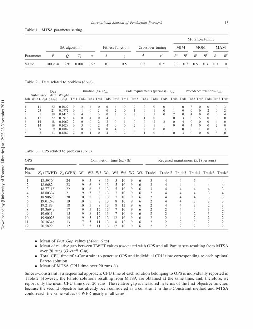
In this section, the performance of the proposed MTSA to solve the considered problem is investigated using anumber of test problems adopted from real data. To generate OPS, the proposed model is solved by "-Constraintmethod using LINGO 10.0 software. The used system is an x64-based work station with 8 Intel Xeon processor2.0GHz and 2 GB memory. MTSA is coded by Visual Basic 2008. Six test problems with 8 to 13 jobs and 6 tradesare adopted from the real data related to the daily (24 h) work requests. The detailed information for the first testproblem with M¼ 8 jobs and K¼ 6 trades (or 8� 6 for short) is presented in Table 2. In the section ‘PrecedenceRelations’ in Table 2, a non-zero entry q in row m and column k means trade q is prior to trade k to do job i. TheOPS associated with example (8� 6) resulting from "-Constraint algorithm is shown in Table 3. In total, 12 Paretosolutions are obtained; this illustrates the scheduling of the jobs is not possible with fewer than 12 maintainers andthe best result can be achieved by 24 maintainers. In other words, the flow time of the jobs will not be improved evenif more than 24 maintainers are employed. The Pareto front corresponding to the OPS presented in Table 1 isgraphically shown in Figure 7; the trade-off between TWFT and workforce requirements (WFR) is clearlydemonstrated. As is evident in this figure, when the total number of available maintainers decreases, TWFTincreases with an ascending trend. For further discussion, refer to Safaei et al. (2011).

To compare the performance of "-Constraint and MTSA, the six test problems resulting in 90 Pareto solutionsare solved using both approaches. To determine the best combination of MTSA’s parameter, an experimental designis performed in the predefined intervals based on the dynamic tuning strategy explained in Section 4. The bestobtained parameter setting is summarised in Table 1.

The MTSA is run 20 times for each test problem, and the following outputs are reported in Table 4:

. OPS resulting from "-Constraint and the best Pareto set (BPS) resulting from MTSA

. Relative gap between TWFT values associated with OPS and BPS (Best_Gap)

Figure 7. Optimal Pareto frontier for problem 8� 6.

12 N. Safaei et al.

Dow

nloa

ded

by [

Uni

vers

ity o

f T

oron

to L

ibra

ries

] at

12:

25 2

5 N

ovem

ber

2011

. Mean of Best_Gap values (Mean_Gap)

. Mean of relative gap between TWFT values associated with OPS and all Pareto sets resulting from MTSAover 20 runs (Overall_Gap)

. Total CPU time of "-Constraint to generate OPS and individual CPU time corresponding to each optimalPareto solution

. Mean of MTSA CPU time over 20 runs (s).

Since "-Constraint is a sequential approach, CPU time of each solution belonging to OPS is individually reported inTable 2. However, the Pareto solutions resulting from MTSA are obtained at the same time, and, therefore, wereport only the mean CPU time over 20 runs. The relative gap is measured in terms of the first objective functionbecause the second objective has already been considered as a constraint in the "-Constraint method and MTSAcould reach the same values of WFR nearly in all cases.

Table 3. OPS related to problem (8� 6).

OPS Completion time (’m) (h) Required maintainers (�k) (persons)

ParetoNo. Z1 (TWFT) Z2 (WFR) W1 W2 W3 W4 W5 W6 W7 W8 Trade1 Trade 2 Trade3 Trade4 Trade5 Trade6

1 18.59104 24 9 5 8 13 5 10 9 6 3 4 4 5 4 42 18.66824 23 9 6 8 13 5 10 9 6 3 4 4 4 4 43 18.77118 22 10 6 8 13 5 10 9 6 3 4 4 4 4 34 18.80334 21 9 5 8 13 7 10 9 6 2 4 4 4 3 45 18.90628 20 10 5 8 13 7 10 9 6 2 4 4 4 3 36 19.01243 19 10 5 8 13 8 10 9 6 2 4 4 3 3 37 19.2183 18 10 5 8 13 8 12 9 6 2 4 4 3 2 38 19.36949 17 9 5 12 13 7 10 9 6 2 2 4 4 3 29 19.6011 15 9 8 12 13 7 10 9 6 2 2 4 2 3 210 19.90025 14 9 5 12 13 12 10 9 6 2 2 4 2 2 211 20.36346 13 17 5 11 13 8 12 9 6 2 2 2 3 2 212 20.5822 12 17 5 11 13 12 10 9 6 2 2 2 2 2 2

Table 2. Data related to problem (8� 6).

JobSubmissiondate (- rm)

Duedate(þdm)

Weight(wm)

Duration (h) - ptmk Trade requirements (persons) -Wmk Precedence relations - pmkl

Trd1 Trd2 Trd3 Trd4 Trd5 Trd6 Trd1 Trd2 Trd3 Trd4 Trd5 Trd6 Trd1 Trd2 Trd3 Trd4 Trd5 Trd6

1 11 22 0.1029 0 2 4 0 0 4 0 2 2 0 0 1 0 3 0 0 0 32 23 21 0.0772 0 1 0 3 0 2 0 1 0 1 0 1 0 0 0 2 0 23 5 19 0.1415 0 4 0 3 0 2 0 2 0 1 0 2 0 4 0 0 0 44 15 22 0.0918 4 0 4 0 4 0 1 0 1 0 1 0 3 0 5 0 0 05 14 18 0.1062 2 0 0 2 2 0 1 0 0 2 2 0 4 0 0 0 4 06 14 19 0.1029 0 3 0 2 4 0 0 2 0 1 1 0 0 4 0 0 2 07 9 9 0.1887 2 0 2 0 0 4 2 0 2 0 0 1 0 0 1 0 0 38 5 13 0.1887 2 0 1 0 4 0 2 0 1 0 1 0 3 0 0 0 3 0

Table 1. MTSA parameter setting.

SA algorithm Fitness function Crossover tuning

Mutation tuning

MIM MOM MAM

Parameter P Q Tf � � � rI rF RI RF RI RF RI RF

Value 100�M 250 0.001 0.95 10 0.5 0.8 0.2 0.2 0.7 0.5 0.3 0.3 0

International Journal of Production Research 13

Dow

nloa

ded

by [

Uni

vers

ity o

f T

oron

to L

ibra

ries

] at

12:

25 2

5 N

ovem

ber

2011

Table 4. Comparison between MTSA and "-Constraint method.

"-Constraint MTSA

ProblemParetoNo.

Z1

(TWFT)Z2

(WFR)CPU

time (s)Z1

(TWFT)Z2

(WFR)Mean CPUtime (s)

Best_Gap(%)

OverallGap (%)

8� 6 1 18.59104 24 1 18.59104 24 39.2 0 0.8672 18.66824 23 1 18.66824 23 03 18.77118 22 2 18.77118 22 04 18.80334 21 2 18.80334 21 05 18.90628 20 2 18.90628 20 06 19.01243 19 2 19.01243 19 07 19.2183 18 10 19.30194 18 0.4338 19.36949 17 6 19.51424 17 0.7429 19.6011 15 10 19.94529 15 1.72610 19.90025 14 24 20.20906 14 1.52811 20.36346 13 43 20.37633 13 0.06312 20.5822 12 43 20.74356 12 0.778

Total¼ 146 Mean gap ! 0.439

9� 6 1 19.25899 27 1 19.25899 27 51.15 0 1.1462 19.34622 26 1 19.34622 26 03 19.38415 25 1 19.43345 25 0.2544 19.5093 23 1 19.5093 23 05 19.64583 22 2 19.6608 22 0.0766 19.77099 21 5 19.77098 21 07 19.92249 20 9 19.92249 20 08 20.07228 19 9 20.19914 19 0.6289 20.19744 18 14 21.01763 18 3.90210 20.71146 17 16 21.1074 17 1.87611 21.31309 16 17 21.32063 16 0.03512 21.82711 15 24 21.95981 15 0.604

Total¼ 100 Mean gap! 0.614

10� 6 1 26.87772 25 1 26.95793 25 54.09 0.298 1.3502 26.95993 24 1 27.04014 24 0.2973 27.04215 23 1 27.19855 23 0.5754 27.21501 22 3 27.28077 22 0.2415 27.36298 21 5 27.36509 21 0.0086 27.44731 20 6 27.45152 20 0.0157 27.61595 19 13 27.78671 19 0.6158 27.78038 18 20 28.4249 18 2.2679 27.98591 17 20 28.44272 17 1.60610 28.25978 16 36 28.64826 16 1.35611 28.76571 15 38 - - -12 29.40526 14 40 - - -

Total¼ 184 Mean gap! 0.727

11� 6 1 20.958384 32 1 20.95838 32 79.5 0 1.1872 21.031986 31 1 – – *3 21.031986 30 1 21.03199 30 04 21.146278 29 1 21.14838 29 0.015 21.206579 28 2 21.22512 28 0.0876 21.278078 27 3 21.29873 27 0.0977 21.368238 26 7 21.36824 26 08 21.484633 25 15 21.55108 25 0.3089 21.556132 24 37 21.64045 24 0.3910 21.685229 23 38 21.88868 23 0.92911 21.800958 22 86 22.02771 22 1.02912 22.033748 21 425 22.09722 21 0.28713 22.186596 20 326 22.1866 20 0

(continued )

14 N. Safaei et al.

Dow

nloa

ded

by [

Uni

vers

ity o

f T

oron

to L

ibra

ries

] at

12:

25 2

5 N

ovem

ber

2011

The obtained results are satisfactory and, indeed, are very promising from both CPU time and solution qualitypoints of view. For 90 Pareto solutions, the average of Overall_Gap is about 1% while the average of Best_Gap is0.65%. Moreover, the CPU time of MTSA is practically negligible compared to the exact approach. For instance, asshown in Table 4, the total time required to generate OPS for problems (12� 6) and (13� 6) was about 9.5 h and

Table 4. Continued.

"-Constraint MTSA

ProblemParetoNo.

Z1

(TWFT)Z2

(WFR)CPU

time (s)Z1

(TWFT)Z2

(WFR)Mean CPUtime (s)

Best_Gap(%)

OverallGap (%)

14 22.373846 19 1329 22.46862 19 0.42215 22.542975 18 579 22.74668 18 0.89616 22.779221 17 1364 23.10854 17 1.42517 23.070208 16 1910 23.3866 16 1.35318 23.414404 15 1363 23.79133 15 1.58419 23.91144 14 2090 24.05337 14 0.5920 24.402293 13 471 25.19203 13 3.135

Total¼ 10,049 Mean gap! 0.660

12� 6 1 22.51672 31 0 22.51672 31 92.4 0 1.4982 22.60079 30 0 22.60079 30 03 22.71289 29 3 22.73927 29 0.1164 22.73113 28 1 22.76894 28 0.1665 22.8152 27 8 22.83256 27 0.0766 22.92587 26 19 - - *7 22.92587 25 14 22.93708 25 0.0498 22.9895 24 27 23.00071 24 0.0499 23.12797 23 39 23.15963 23 0.13710 23.30442 22 236 23.30442 22 011 23.47257 21 558 23.58466 21 0.47512 23.72313 20 1464 23.80886 20 0.3613 23.89128 19 6489 23.94733 19 0.23414 24.06503 18 4320 24.24581 18 0.74615 24.32493 17 8471 25.39587 17 4.21716 24.56912 16 8132 25.48653 16 3.617 24.94837 15 2720 25.518 15 2.23218 25.41996 14 1112 25.625 14 0.819 25.84528 13 419 26.11119 13 1.018

Total: 9:30 h Mean gap! 0.793

13� 6 1 23.45482 37 1 23.45482 37 103.25 0 0.9343 23.50966 35 1 23.50966 35 04 23.60741 34 1 23.60741 34 0.4145 23.61423 33 1 23.61423 33 0.0296 23.71198 32 34 23.71198 32 0.4127 23.77482 31 37 23.77482 31 0.2648 23.83868 30 63 23.87257 30 0.4099 23.91679 29 273 23.9168 29 0.32710 23.94325 28 341 24.02386 28 0.44611 24.041 27 284 24.07739 27 0.55712 24.18349 26 1800 24.38588 26 1.41413 24.28125 25 9842 24.49051 25 1.25414 24.42176 24 11304 24.59758 24 1.28615 24.6238 23 23769 24.96216 23 2.16516 N/A 22 412 hours 25.09111 22 1.86217 N/A 21 412 hours 25.5641 21 N/A18 N/A 20 412 hours 26.0233 20 N/A

Total:424 h Mean gap! 0.722

International Journal of Production Research 15

Dow

nloa

ded

by [

Uni

vers

ity o

f T

oron

to L

ibra

ries

] at

12:

25 2

5 N

ovem

ber

2011

more than 14 h, respectively, whilst MTSA reached near-optimal Pareto sets within 94 s and 103 s, respectively,which is very satisfactory. The OPS versus the Pareto sets resulting from MTSA over 20 runs for problems (12� 6)and (13� 6) are graphically shown in Figures 8 and 9 respectively. In test problem 13� 6, the four last Paretosolutions cannot be individually obtained within 12 h; however, based on MTSA results, we have determined thatthese solutions exist. The trend of the optimal Pareto front in Figure 9 indicates that the MTSA outputs and themissed part of OPS for (12� 6) and (13� 6) are very close. One interesting issue in the computational aspect of theproposed MTSA is that by decreasing the size of the available workforce, CPU time increases progressively as isevident in Table 2. When workforce size is decreased, the number of feasible workforce allocations increasesprogressively in a given schedule. From the mathematical programming point of view, the decreasing of theworkforce size greatly increases the number of non-zero variables ykmn in Constraint (10), and this results in a largeincrease of search space in the B&B method.

Figure 8. Optimal Pareto front versus Pareto fronts resulted from MTSA during 20 runs – problem (12� 6).

Figure 9. Optimal Pareto front versus Pareto fronts resulted from MTSA during 20 runs – problem (13� 6).

16 N. Safaei et al.

Dow

nloa

ded

by [

Uni

vers

ity o

f T

oron

to L

ibra

ries

] at

12:

25 2

5 N

ovem

ber

2011

6. Conclusions

In this article, a simulated annealing algorithm with parallel architecture, so-called multi-threading simulatedannealing (MTSA), is proposed to solve a bi-objective maintenance scheduling problem with a multi-skilledworkforce constraint. In the considered problem, a central department is responsible for scheduling the maintenancejobs submitted by different manufacturing areas throughout the plant. The jobs have different priorities, and thereare some precedence relations between different skills in carrying out the jobs. The problem has been alreadyformulated as a bi-objective mixed-integer programming model to simultaneously minimise equipmentunavailability and workforce requirements. The total weighted flow time is used as a scheduling criterion tomeasure equipment availability.

The proposed MTSA supposes that the optimal Pareto set (OPS) is a bi-section curve so that each section will beconstructed by a thread. Thus, each thread has its own Pareto archive, and there is no interaction between thethreads. This property represents the greatest advantage of the proposed MTSA, because CPU time significantlydecreases whilst the size of the common region being searched by both threads is significantly reduced.

The performance of the proposed MTSA is considerable in terms of both solution quality and computationaleffort. The proposed MTSA has the ability to search the whole objective space in a reasonable time so that theaverage of the relative Gap between OPS and Pareto set resulting fromMTSA is about 1%, while the computationaleffort of MTSA is practically negligible when compared to the exact approach. The multi-threading strategy can beapplied to other meta-heuristics, such as evolutionary algorithms, to solve the considered problem. Moreover, themulti-threading architecture may be used to hybridise several meta-heuristics together as a powerful solutionstrategy. However, the optimal number of used threads will be a challenging issue.

Acknowledgement

Our sincere thanks go to Elizabeth Thompson from C-MORE Lab for her careful editing.

Note

1. Computerised maintenance management system.

References

Ahire, S., et al., 2000. Workforce-constrained preventive maintenance scheduling using evolution strategies. Decision Science

Journal, 31 (4), 833–859.Batouche, M., Meshoul, S., and Abbassene, A., 2006. On solving edge detection by emergence. Lecture Notes in Computer

Science, 4031, 800–808.Evjen, B., et al., 2008. Professional visual basic 2008. India: Wiley.

Gopalakrishnan, M., Ahire, S.L., and Miller, D.M., 1997. Maximizing the Effectiveness of a preventive maintetance system: an

adaptive modelling approach. Management Science, 43 (6), 827–840.Higgins, A., 1998. Scheduling of railway track maintenance activities and crews. Journal of the Operational Research Society, 49,

1026–1033.Marmier, F., Varnier, C., and Zerhouni, N., 2009. Proactive, dynamic and multi-criteria scheduling of maintenance activities.

International Journal of Production Research, 47 (8), 2185–2201.Miettinen, K.M., 1999. Nonlinear multiobjective optimization. Kluwer Academic.Mjema, E., 2002. An analysis of personnel capacity requirement in the maintenance department by using a simulation method.

Journal of Quality Maintenance Engineering, 8 (3), 253–273.

Moore, W.J. and Starr, A.G., 2006. An intelligent maintenance system for continuous cost-based prioritization of maintenance

activities. Computers in Industry, 57 (6), 595–606.Lazarova, M., 2008. Parallel simulated annealing for solving the room assignment problem on shared and distributed memory

platforms, ACM International Conference Proceeding Series Vol. 374(2), Proceedings of the 9th International Conference on

Computer Systems and Technologies and Workshop for PhD Students in Computing, Gabrovo, Bulgaria, 2008, 1–6.Quan, G., et al., 2007. Searching for multiobjective preventive maintenance schedules: combining preferences with evolutionary

algorithms. European Journal of Operational Research, 177 (3), 1969–1984.Quere, Y.L., et al., 2003. Reactive scheduling of complex system maintenance in a cooperative environment with communication

times. IEEE Transactions on Systems, Man, and Cybernetics—Part C: Applications and Reviews, 33 (2), 225–234.

International Journal of Production Research 17

Dow

nloa

ded

by [

Uni

vers

ity o

f T

oron

to L

ibra

ries

] at

12:

25 2

5 N

ovem

ber

2011

Ram, D.J., Sreenivas, T.H., and Subramanian, K.G., 1996. Parallel simulated annealing algorithms. Journal of Parallel andDistributed Computing, 37 (2), 207–212.

Roberts, S.M. and Escudero, L.F., 1983. Scheduling of plant maintenance personnel. Journal of Optimization Theory andApplications, 39 (3), 323–343.

Safaei, N., Banjevic, D., and Jardine, A.K.S., 2008. Multi-objective simulated annealing for a maintenance workforce schedulingproblem: a case study. In: Cher Ming Tan, ed. Global optimization: focus on simulated annealing. Vienna, Austria: ARS

Publishing, 27–48.Safaei, N., Banjevic D., and Jardine, A.K.S., 2011. Workforce-constrained maintenance scheduling: a case study. Journal of

Operational Research Society, 62, 1005–1018.

Sohn, A., 1995. Parallel N-ary speculative computation of simulated annealing. IEEE Transactions on Parellel and DistributedSystems, 6 (10), 997–1005.

Talbi, E.G., et al., 2008. Parallel approaches for multiobjective optimization. Lecture Notes in Computer Science, 5252, 349–372.

Tavakkoli-Moghaddam, R., et al., 2005. Solving a dynamic cell formation problem using metaheuristics. Applied Mathematicsand Computation, 170 (2), 761–780.

Vergin, R.C., 1966. Scheduling maintenance and determining crew size for stochastically failing equipment. Management Science,13 (2), 52–65.

Wagner, H.M, Giglio, R.J., and Glaser, R.G., 1964. Preventive maintenance scheduling by mathematical programming.Management Science, 10 (2), 316–334.

Wittenburg, J.P., Pirsch, P., and Meyer, G, 1999, A multithreaded architecture approach to parallel DSPs for high performance

image processing applications, IEEE Workshop on Signal Processing Systems (SiPS 99), 20–22 Oct, 241–250.Worrall, B. M. and Mert, B., 1980. Application of dynamic scheduling rules in maintenance planning and scheduling.

International Journal of Production Research, 18 (1), 57–71.

Yanga, T-H., Yanb, S., and Chen, H-H., 2003. An airline maintenance manpower planning model with flexible strategies.Journal of Air Transport Management, 9, 233–239.

Zalzala, A.M.S. and Green, D., 1999. MTGP: a multithreaded Java tool for genetic programming applications. Proceedings of

Congress on Evolutionary Computation (CEC), 2, 904–911.

18 N. Safaei et al.

Dow

nloa

ded

by [

Uni

vers

ity o

f T

oron

to L

ibra

ries

] at

12:

25 2

5 N

ovem

ber

2011