Multiple Ecosystem Markets 

in Maryland:  

Quantifying the Carbon Benefits  Associated with Nutrient Trading 

 A study commissioned by 

The Maryland Department of the Environment  

Center for Integrative Environmental Research (CIER) University of Maryland 

 In collaboration with  

World Resources Institute (WRI)  

December 2010 

 

Research Team  University of Maryland Rebecca Gasper Graduate Research Assistant, Center for Integrative Environmental Research,  Gwen Bagley Graduate Research Assistant, Center for Integrative Environmental Research,  Matthias Ruth Director, Center for Integrative Environmental Research, and Roy F. Weston Chair for Natural Economics  World Resources Institute Mindy Selman Senior Associate  Liz Marshall Former Senior Economist 

  

 We wish to thank the Maryland Department of the Environment for their support of this research.   Cover Photo: Jane Thomas, IAN Image Library                            (ian.umces.edu/imagelibrary/)   The Center for Integrative Environmental Research (CIER) at the University of Maryland addresses complex environmental challenges through research that explores the dynamic interactions among environmental, economic and social forces and stimulates active dialogue with stakeholders, researchers and decision makers. Researchers and students at CIER, working at local, regional, national and global scales, are developing strategies and tools to guide policy and investment decisions. For additional information, please visit www.cier.umd.edu.

 

 

1 | P a g e

Contents Executive Summary .................................................................................................................................. 2 

Key Findings ..................................................................................................................................... 4Scenarios Analyzed ........................................................................................................................... 2 

Future Research................................................................................................................................. 4 

Glossary .................................................................................................................................................... 5 

List of Acronyms and Units ...................................................................................................................... 6 

List of Figures ........................................................................................................................................... 6 

List of Tables ............................................................................................................................................ 7 

Introduction ............................................................................................................................................... 9 

Model Development ................................................................................................................................ 12 

Modeling Best Management Practices (BMPs) .............................................................................. 13 

Scenario descriptions ...................................................................................................................... 15 

Scenario analysis ............................................................................................................................. 18 

Results ..................................................................................................................................................... 18 

Expected carbon benefits from water quality trading ..................................................................... 18 

Marketable carbon........................................................................................................................... 19 

Market rules and carbon supply ...................................................................................................... 20 

Capturing true project costs ............................................................................................................ 22 

Market prices of carbon .................................................................................................................. 23 

Conclusion .............................................................................................................................................. 24 

References ............................................................................................................................................... 24 

Appendices .............................................................................................................................................. 26 

Appendix A. Markets for Ecosystem Services: Principles, Objectives, Designs, and Dilemmas ...... 26 

A.1 Background and Introduction ................................................................................................... 26 

A2. Markets for Ecosystem Services .............................................................................................. 29 

A3. Ecosystem Services Markets and Environmental Improvement .............................................. 35 

A4. Ecosystem Services and Multiple Markets .............................................................................. 37 

A5. Regulatory Approaches to Multiple Markets ........................................................................... 45 

A6. Conclusion ............................................................................................................................... 52 

A7. References ................................................................................................................................ 53 

Appendix B. ........................................................................................................................................ 56 

B1. Introduction .............................................................................................................................. 56 

B2. Water Quality Trading Markets in the Chesapeake Bay .......................................................... 58 

B3.Voluntary and Regulatory Carbon Markets .............................................................................. 68 

Appendix C. Model Description ......................................................................................................... 79  

C1. Model overview ........................................................................................................................ 79 

2 | P a g e

Executive Summary Maryland recently established a nutrient trading program for nonpoint sources in the state to improve water quality in the Chesapeake Bay and its tributaries1. This program uses a market (i.e. a platform for trading goods and services) for nutrients to create an incentive for sources to reduce water pollution at low cost. To reach targets for nitrogen and phosphorous, nonpoint sources implement projects from a suite of best management practices (BMPs) that reduce the amounts of nutrients that enter nearby water sources. Examples of BMPs include conservation buffers, conservation tillage, cover crops and wetland restoration among others. Once sources have reduced nutrient loading levels beyond the Total Maximum Daily Load (TMDL) allocations specified in Maryland’s Tributary Strategy, they can sell additional load reductions as credits to those sources that remain above their TMDLs. Many of the BMPs that improve water quality by removing nutrients from runoff also have ancillary carbon benefits – they sequester carbon dioxide from the atmosphere. This creates the possibility for sources to generate credits for sale in two different markets (water quality and carbon) with a single project, a process known as stacking. There is currently some debate whether stacking can compromise the environmental integrity of markets because it may reward carbon reductions that are not truly additional, meaning that they would have occurred even if the market had not been created. Rules and stipulations regarding participation in multiple markets have been developed to maintain the environmental integrity of markets while also preserving their potential to incentivize pollution reduction. Since the concept of developing markets for multiple ecosystem services is relatively new, however, there are few reliable case studies and little empirical data upon which to develop rules for Maryland’s trading program. As a step toward informing the development of Maryland’s Nutrient Trading with Carbon Benefits plan, this study evaluates the following two primary questions:

• What are the carbon benefits (measured as carbon sequestration potential) associated with Maryland’s nutrient trading market?

• What relative marketable carbon supply can be expected from this plan given a variety of market rules and stipulations designed to ensure that all marketable carbon is truly additional?

To answer these questions, the Center for Integrative Environmental Research (CIER) together with the World Resources Institute (WRI) developed a dynamic systems model of agriculture in the state of Maryland to calculate carbon sequestration and marketable supply resulting from the nutrient trading program through 2030.

Scenarios Analyzed Given the many potential variations for such a program, we modeled three different Market Scenarios subject to three different overarching Baseline Scenarios for the five major watershed basins in MD (Susquehanna, Eastern Shore, Western Shore, Patuxent, Potomac). This resulted in the six unique sets of rules described in Table E1.

1 See Maryland Climate Action Plan, AFW-8, http://www.mde.state.md.us/assets/document/Air/ClimateChange/Appendix_D_Mitigation.pdf

3 | P a g e

Table E 1 Market participation rules for each combination of Market Scenario (MS) and Baseline Scenario (BS). Each of the six scenarios was run for all possible combinations of nutrient and carbon prices from $5-10 to assess marketable carbon supply through 2030.

BS MS

TMDL Baseline (1)

No Baseline (2)

Credit Retirement (3)

Stacking Permitted (1)

Before TMDL is reached, source will not participate in either market After TMDL is reached, source implements cost-effective BMPs and participates in both markets

Before TMDL is reached, source participates in the carbon market Before TMDL is reached, source participates in the carbon market

Conditions are always the same as in the No Baseline (2) Scenario, but only 75% of credits are added to the market supply of carbon because 25% are retired toward MD’s emission reduction goal.

Stacking Never Permitted (2)

Before TMDL is reached, source will not participate in either market After TMDL is reached, source implements cost-effective BMPs and participates in whichever market (carbon or nutrient) gives a larger anticipated return

Before TMDL is reached, landowner will participate in the carbon market After TMDL is reached, source continues to implement cost-effective BMPs and participates in whichever market (carbon or nutrient) gives a larger anticipated return

Financial Additionality (3)

Before TMDL is reached, source will not participate in either market After TMDL is reached, source implements cost-effective BMPs and participates in both carbon and nutrient markets for eligible projects. For those projects not eligible for stacking but still cost-effective, he will participate in the market that gives a larger anticipated return

Before TMDL is reached, source participates in the carbon market After TMDL is reached, source implements cost-effective BMPs and participates in both carbon and nutrient markets for eligible projects. For those projects not eligible for stacking but still cost-effective, he will participate in the market that gives a larger anticipated return

The three Baseline Scenarios determined if sources were subject to a baseline requirement before participating in the carbon market: 1) Sources must meet the nutrient TMDL before participating in the carbon market; 2) No baseline for participation in the carbon market; 3) No baseline for participation in the carbon market, but 25 percent of carbon credits generated by a project must be retired toward Maryland’s goal of reducing greenhouse gas emissions 25 percent by 2020. The Market Scenarios determined whether or not sources could participate in multiple markets with the same BMP: 1) Credit

4 | P a g e

stacking permitted; 2) Credit stacking not permitted, sources must choose to participate in either the nutrient or the carbon market; 3), Financial additionality applies, which only permits stacking when the cost of a BMP is not covered by a single market alone. We then simulated each scenario under every possible combination of market price for nutrients and carbon from $5/credit to $50/credit. For each scenario we calculated carbon sequestration and the magnitude of marketable carbon supply. We also developed carbon supply curves that show the relationship between carbon credit market price and the quantity of carbon supplied to the market.

Key Findings 1. Expected carbon sequestration due to the nutrient trading policy reaches between 1.01-1.78

million metric tons of carbon per year by 2030. 2. Total cumulative carbon sequestration due to the nutrient trading policy is expected to reach

between 12.5-21.6 million metric tons of carbon by 2030. 3. Of the carbon sequestered, roughly 7 percent is marketable in the TMDL Baseline Scenario (BS

1), 23 percent is marketable in the No Baseline Scenario (BS 2), and 17 percent is marketable in the Credit Retirement Scenario (BS 3).

4. Market rules and requirements influence the shape of the carbon supply curve and, therefore, how sensitive the amount of carbon supplied is to changes in carbon credit price in the market.

a. When nutrient prices are low, quantity of carbon supplied in the market increases as carbon market prices increase for Stacking Permitted (MS 1) and Stacking Never Permitted (MS 2) Scenarios.

b. In contrast, carbon supply in the Financial Additionality Scenario (MS 3) increases with carbon credit prices up to a threshold value (estimated around $25/metric ton carbon) then begins to decrease as fewer projects meet the financial additionality criterion.

c. When nitrogen prices are between $15-20/lb, the quantity of carbon supplied is less sensitive to changes in carbon price.

5. Most BMPs generate more revenue in the nutrient market than carbon market. 6. Carbon prices on average have to be 5-8 times higher than nutrient prices to provide adequate

incentive for sources to choose to participate in the carbon market when stacking is not permitted.

Future Research This study provides insights on expected carbon supply in a market that interacts with a nutrient trading water quality market. We incorporate a range of credit prices to show how carbon supply changes depending both on carbon credit prices and nutrient credit prices. Because this is a supply side analysis, however, we have no way of predicting the value of credit prices in the market over time. Fluctuating prices will of course influence the magnitude of carbon supply and implementation of BMPs. Future research should focus on potential demand for carbon both from regional and potential national markets. When interpreted in tandem with our supply-side results, such studies could provide an idea of what prices to expect in the market in the future and can further inform the development of Maryland’s nutrient trading program.

5 | P a g e

Glossary Additionality – With respect to carbon emissions, reductions that would not have occurred in the absence of a carbon market Carbon market – A specific type of ecosystem market where credits representing carbon emissions are exchanged Market – An economic system in which goods and services are exchanged Ecosystem market – A system in which environmental goods and services (e.g. carbon credits generated from emissions reductions) are exchanged Ecosystem service – A benefit to human societies from naturally existing resources and processes Elastic– The condition of a market supply curve whereby quantity of the good supplied changes rapidly as price changes Externality – Positive or negative impacts of an activity that are not included in the price of the activity Inelastic – The condition of a supply curve whereby quantity of the good supplied does not change as its price changes Market rules – Requirements and stipulations that govern market function, including eligibility for participation in the market as well as use of credits and revenue generated in the market Nonpoint source – A diffuse source of pollution Nutrient Trading with Carbon Benefits – The policy option (AFW-8) described in Appendix D of the Maryland Climate Action Plan that establishes a water quality trading (referred to as nutrient trading) program in MD and emphasizes the potential for projects that improve water quality to simultaneously sequester carbon dioxide from the atmosphere Total Maximum Daily Load - A calculation for an impaired waterbody of the maximum amount of a pollutant the waterbody can receive and still meet applicable water quality standards (accounting for seasonal variations and a margin of safety), including an allocation of pollutant loadings to point sources (WLAs) and nonpoint sources (load allocations (LAs)). Tributary Strategy (TS) Program - Establishes specific nutrient reduction targets for each of these watersheds from every source, including agricultural fields, urban and suburban lands, and wastewater treatment plants Supply Curve – The relationship between price and quantity supplied of a given good in a market Stacking – (Sometimes referred to as ‘credit stacking’ in text) A single project receives more than one payment for more than one associated ecosystem benefit

6 | P a g e

Water quality market – A specific type of ecosystem market where credits representing nutrients (commonly nitrogen and phosphorus) emitted into water sources are exchanged

List of Acronyms and Units BMP – Best Management Practice BS – Baseline Scenario C - Carbon CO2 – Carbon dioxide CBP – Chesapeake Bay Program CCX – Chicago Climate Exchange CREP – Conservation Reserve Enhancement Program EPA – Environmental Protection Agency MACS – Maryland Agricultural Water Quality Cost Share MDA – Maryland Department of Agriculture MDE – Maryland Department of the Environment MS – Market Scenario Mt – Metric tons N - Nitrogen OTC – Over the Counter RGGI – Regional Greenhouse Gas Initiative TMDL – Total Maximum Daily Load TS – Tributary Strategy USDA – United States Department of Agriculture

List of Figures Figure 1 Schematic of primary model sectors with descriptions of inputs and data sources. CBP=Chesapeake Bay Program; USDA=United States Department of Agriculture; MDE=Maryland Department of Agriculture; EPA= Environmental Protection Agency. Squares represent exogenous variables (i.e., set by the user of the model) and rounded corners represent endogenous variables (i.e., calculated within the model). .................................................................................................................. 12 Figure 2 Decision-making process used by the model each year to simulate BMP implementation within each basin (Susquehanna, Eastern Shore, Western Shore, Patuxent, Potomac) for each land use category (high till, low till, manure). ...................................................................................................... 13 Figure 3 Decision-making process for Market Scenario 1 (stacking permitted) after relevant baselines have been achieved. ................................................................................................................................ 16 Figure 4 Decision-making process for Market Scenario 2 (stacking not permitted) after relevant baselines have been achieved. ................................................................................................................. 17 Figure 5 Decision-making process for Market Scenario 3 (financial additionality) after relevant baselines have been achieved. ................................................................................................................. 18 Figure 6 Total carbon sequestered (Metric tons – Mt) each year from all BMPs as a result of Maryland's nutrient trading policy. ......................................................................................................... 19 Figure 7 Marketable carbon (Mt) supply under three rules for market participation: No baseline, 25% Banking (25% of carbon credits generated from any project must be banked) and Baseline (nutrient TS sets the carbon baseline). ........................................................................................................................ 20 Figure 8 Relative carbon supply curves showing the relationship between price of carbon, P(C), and quantity of carbon supplied in the market, Q(C), subject to three different market additionality rules: S1

7 | P a g e

= Market Scenario 1 (Stacking), S2= Market Scenario 2 (No Stacking), S3 = Market Scenario 3 (Financial Additionality). Panel (a) shows supply under low nitrogen prices ($5-10/lb N) and panel (b) shows supply under mid-range nitrogen prices ($15-20/lb N). .............................................................. 21 

Figure A. 1 MEA categorization of ecosystem services. ........................................................................ 27 

 Figure A. 2 PES refer to a suite of incentive-based mechanisms that operate within a broader framework of environmental policy instruments. (Source: Jack et al. 2008). ........................................ 28 

Figure A. 4 Theoretical market equilibrium ........................................................................................... 40Figure A. 3 Financial additionality criterion. (Source: Bianco, 2009) ................................................... 40 

Figure A. 5 Supply and demand for nutrient credits ............................................................................... 41 

Figure A. 6 Supply and demand for nutrient credits ............................................................................... 41 

Figure A. 7 Supply and demand for nutrient credits with an interacting carbon credit (CC) market. .... 42 

Figure A. 8 Supply and demand with baseline performance requirements. ........................................... 43  

Figure A. 9 A buyer, investment seller framework for ecosystem services (Binning 2002) .................. 46  Figure C. 1 Sample model run to show BMP cost variation. The BMP modeled here is a forest buffer with an imposed normal cost distribution (mean=$800/acre; SD=$25/acre). ........................................ 81 Figure C. 2 Sample carbon supply curve generation in a low nitrogen price ($5-10/credit) environment when stacking is permitted. Simulation output of aggregate supplied carbon from panel (a) are used to graphically create the general supply curve shown in panel (b) of quantity supplied, Q(C), at different carbon prices, P(C). ................................................................................................................................. 83 

List of Tables Table 1 Tributary Strategies, nitrogen loading levels, and reduction required from 2008 levels to meet the Tributary Strategy goals for agriculture and manure nonpoint sources by basin for Maryland. ...... 11 Table 2 BMP nutrient reduction effectiveness, carbon sequestration potential and costs for those BMPs that could be used to generate carbon credits (Data: EPA, USDA, MDA). Costs are listed as Not Applicable (N/A) for those BMPs that are not considered marketable. ................................................. 14 Table 3 Total and cumulative carbon benefits (measured in '000 Mt) under a range of low to high carbon sequestration rates for BMPs ...................................................................................................... 19 Table 4 Break-even prices for nitrogen (N) and carbon (C) when stacking is not permitted. ................ 22 Table 5 Break-even prices for nitrogen (N) and carbon (C) under three cost scenarios: (1) the landowner incurs the entire cost including rental payments; (2) the landowner incurs the full cost not including rental payments; and (3) 50% of the entire project including soil rent is covered by cost share. ................................................................................................................................................................. 23 

Table B.1 GHG co-benefits of BMPs eligible in nutrient trading markets ............................................. 57 

 

Table B.3 State Trading Basins ............................................................................................................... 63Table B.2 State Water Quality Trading Programs .................................................................................. 61 

Table B.4 Current State Baseline Requirements for Agriculture ............................................................ 64 

Table B.5 Best management practices and associated nutrient efficiencies ........................................... 66 

Table B.6 Carbon Offset Prices (2008) ................................................................................................... 68  

Table B.7 CCX Offset registration ......................................................................................................... 73 

Table C. 1 Data sources for model parameters ....................................................................................... 80  

 Table C. 2 Nitrogen edge of stream (EOS) factors for modeled basins in MD. (Data source: CBP) ..... 80 

8 | P a g e

Table C. 3 Historical BMP implementation and average implementation rates for modeled BMPs: Conservation tillage (cons tillage), cover crops, forest buffers (FB), grass buffers (GB), wetland restoration (wetland) and manure management (manure). Values in grey are not included in the averagerate calculation. Acreage data were provided by CBP. ........................................................................... 81

 

Table C. 4 BMP carbon sequestration ranges used in model (Sources: USDA, ERS TB 1909, EPA) .. 82 

 

9 | P a g e

Introduction Maryland recently established a nutrient trading program to improve the water quality of the Chesapeake Bay and its tributaries. Some of the management practices that can be used to improve water quality by removing harmful nutrients from nonpoint sources have other environmental benefits, including sequestration of carbon dioxide (CO2) from the atmosphere. The potential exists for sources that use these practices to participate in multiple markets including the nutrient trading market as well as regional carbon markets. However, there are few examples of multiple markets in practice to use as guides to design policies that provide incentives that are both economically and environmentally sound. The purpose of this study is to explore how differently structured markets influence the carbon supply that could be generated by practices used by nonpoint sources to meet water quality goals. Specifically, we quantify the carbon sequestration potential associated with Maryland’s nutrient trading program and analyze the magnitude of marketable carbon credits under various market rules. This report is organized as follows: First, we provide a brief background on ecosystem services and the role that markets play in valuing these resources. Second, we describe Maryland’s nutrient trading program and its potential to provide ancillary carbon benefits. Third, we describe and present the results of a modeling analysis undertaken to quantify these benefits and compare carbon supply under a variety of scenarios. Fourth, the report concludes with recommendations for future research that could provide additional insight into the function of markets for multiple ecosystem services in Maryland. Three Appendices are included to supplement the material presented in this report. Appendices A and B were prepared by the World Resources Institute to provide background information and context for the modeling exercise described in the main document. Appendix A provides a comprehensive overview of the concept of markets for multiple ecosystem services, with an emphasis on associated economic and environmental challenges and potential policy tools to address these challenges. Appendix B provides information on water quality and carbon markets in Maryland and throughout the Chesapeake Bay region with a focus on the role of agriculture within these markets. The background in this Appendix can be used to inform discussions of carbon and nutrient stacking in Maryland, as well as to explore potential synergies among states in the future. Appendix C was prepared by CIER as a detailed explanation of the modeling techniques used to conduct the nutrient trading analysis. This Appendix is meant to supplement the methods described in the text with further technical information. Markets for Ecosystem Services2 Ecosystem services are the natural processes and resources that contribute to the functioning of human society, including clean air and water, natural filtration of toxins, and the raw materials we use to harness energy and create goods (de Groot et al. 2002). Most of these vital services are “public goods,” an economics classification referring to resources that are nonrival and nonexcludable (Costanza et al. 1997, Kline et al. 2009). Nonrival means that use of a resource by one individual does not reduce its availability for use by others, and nonexcludable means that nobody can be prevented from using the resource (Marshall and Selman 2010). Any person can breathe clean air, for instance, without reducing the supply available for others to breathe. At the same time, it is not possible to prevent someone from accessing the supply of clean air. Air is both nonrival and nonexcludable and is therefore a public good.

2 For a comprehensive background discussion of markets, see Appendix A.

10 | P a g e

Economic markets, systems in which goods and services are exchanged, theoretically should lead to efficient levels of use and prices of goods through laws of supply and demand. Because public goods are nonrival and nonexcludable, though, the market doesn’t capture them appropriately. One example of a market failure that occurs with respect to public goods is a concept known as an externality, an effect of an activity that is not included in the price of that activity. For example, burning fossil fuels has harmful environmental and human health effects that are not taken into consideration in determining the price of the fuel. Because fuel price is lower than it would be if it included the externalities of health and environmental harm, we tend to use more fuel than we would in a perfectly functioning market. Inefficient use of ecosystem services results in the many examples of environmental degradation we see today. Economists and policy makers try to develop mechanisms to correct these market failures to improve environmental quality. Market-based techniques to improve environmental quality are increasingly being implemented in the United States as complements or alternatives to “command-and-control” approaches. In contrast to command and control methods, which specify how sources must limit pollution, market-based mechanisms attempt to correct the price of various resources and activities so that ecosystem services are efficiently managed. Examples of market mechanisms include fees for use of public goods, subsidies for implementing new technology, and establishment of cap-and-trade programs. Development of markets for ecosystem services is increasingly seen as an effective approach and potential cost reduction tool for those sources operating under regulatory constraints or load caps. In an ecosystem market, sources that reduce pollution below their caps can sell any additional reduction on the market as pollution credits. Sources exceeding their limits can then purchase credits that they need to match their limits with their current levels of pollution. Some practices used to reduce pollution provide more than one environmental benefit. For example, forest and grass buffers planted around agricultural land reduce the amounts of nitrogen and phosphorus that reach local water sources and also remove CO2 from the atmosphere through the biological process of photosynthesis. In theory, sources could undertake an activity known as stacking, participating in more than one market with a single project. Policy makers and economists have been debating whether stacking undermines the environmental integrity of ecosystem markets by allowing sources to generate revenue from carbon reductions that are not truly additional. The concept of additionality means that carbon sequestration occurs as a result of project that would not have been implemented without the existence of the market (Marshall and Selman 2010). If markets honor carbon reductions that are not truly additional, they will not work to correct the externalities that cause inefficient levels of pollution. In this case, using a command and control approach could be more environmentally beneficial. The set of stipulations and requirements for market participation, known as market rules, can be designed to permit only those projects that will result in additional reductions. Establishing a cap or goal, hereafter referred to as a baseline, is a common method of encouraging additionality that requires that certain reductions are made before sources may sell credits in a market. In the case of water quality trading, a watershed TMDL serves as the baseline for credit generation for nitrogen and phosphorous. The TMDL is allocated among all sources in the watershed, and the source must reduce to its assigned allocation. Reductions beyond these allocations are then eligible for sale to other nonpoint or point sources that have not yet reached their assigned TMDL allocation.

11 | P a g e

Designing market rules can be a difficult process in part because it is sometimes impossible to measure additionality or determine if a project is or is not additional. Projects that are potentially eligible in multiple markets are even more challenging because rules must determine the conditions under which stacking is permitted, if it is permitted at all. There have been arguments against allowing stacking based on the premise that stacking rewards benefits that are not truly additional (Bianco 2009). Still, some level of stacking may encourage reductions that would not likely occur under a single ecosystem service market. For example, assume a source has reached its baseline and now the owner of the source must decide whether to implement additional BMPs to generate nutrient or carbon credits. If the most feasible BMP is relatively costly (e.g. installation of a conservation buffer), the owner may not anticipate recovering the cost in the nutrient or the carbon market alone. If stacking in this case is allowed, the owner may anticipate recovering the cost by generating credits for sale in both markets and may implement a BMP he otherwise would not have considered. Water Quality Trading with Carbon Benefits in Maryland Maryland’s water quality standards for the Chesapeake Bay require significant reductions in the amounts of nitrogen and phosphorus that reach the Bay and contribute to poor water quality. Reducing these pollutants has been a major policy focus of Maryland and other states in Chesapeake Bay watershed jurisdictions3. Through the Chesapeake Bay Program, each state has agreed to reduce its contribution of nutrients to the Bay to a specific annual loading level (lbs/year). Each state’s plan for reducing nutrient loads is referred to as its Tributary Strategy (TS). Maryland requires reductions in nutrient loading from nonpoint sources to meet the goals for each basin set in its TS. Table 1 shows TS goals and 2008 nitrogen loading levels for agriculture and manure sources. Table 1 Tributary Strategies, nitrogen loading levels, and reduction required from 2008 levels to meet the Tributary Strategy goals for agriculture and manure nonpoint sources by basin for Maryland.

Basin N loading 2008 (lb N) Tributary Strategy (lb N/yr) Reduction required(%)

Susquehanna 640,277 361, 040 56 Eastern Shore 9,878,244 4,982,612 50 Western Shore 1,138,058 655,835 58 Patuxent 525,565 216,428 41 Potomac 4,677,929 2,689,643 57

In April 2008, Governor O’Malley approved the Nutrient Trading with Carbon Benefits (AFW-8) policy of the Maryland Climate Action Plan Appendix D-14. This strategy encourages adoption of land use management that reduces nutrient loading through the establishment of a water quality trading program. To generate nutrient credits to sell in the market, farmers implement projects that reduce nutrient runoff from a suite of Best Management Practices (BMPs), including conservation buffers, conservation tillage, cover crops and wetland restoration among others. The plan emphasizes the potential of these BMPs to confer ancillary carbon benefits through carbon sequestration, although unresolved issues regarding baselines remain. While some general estimates on the magnitude of the carbon benefits for the nutrient trading policy in have been calculated, no studies to date have used dynamic modeling techniques to calculate these

3 For an overview of the technical details of existing nutrient trading programs in the Chesapeake Bay states, see Appendix B. 4 The final plan was released to the public in August 2008

estimates more accurately. Moreover, no studies to our knowledge have examined the effects of differing water quality market rules on the magnitude of marketable carbon supply. To aid the development of a policy governing markets for projects with multiple ecosystem benefits and associated rules, this study focuses on the following questions: 1) what are the carbon benefits associated with the Maryland nutrient trading policy? and 2) what is the relative carbon supply generated under various market rules?

Model Development To answer the questions described above, we developed a dynamic systems model to simulate nutrient loading in Maryland5. The model was constructed at the watershed basin (hereafter referred to as basin) level for ease of data use, since the most comprehensive data available from the Chesapeake Bay Program are at this level. The five major basins in the state are Susquehanna, Eastern Shore, Western Shore, Patuxent, and Potomac. Figure 1 shows the primary sets of endogenous (i.e. calculated by the model) and exogenous (i.e. set by the model user) variables and their relationships within our model. The land use sector of the model simulates three land use categories (high till, low till and manure) in each basin and the pre-BMP loading level for nitrogen based on historical loading levels calculated from the Chesapeake Bay Program data.

Figure 1 Schematic of primary model sectors with descriptions of inputs and data sources. CBP=Chesapeake Bay Program; USDA=United States Department of Agriculture; MDA=Maryland Department of Agriculture; EPA= Environmental Protection Agency. Squares represent exogenous variables (i.e., set by the user of the model) and rounded corners represent endogenous variables (i.e., calculated within the model).

Figure 2 demonstrates the decision-making process the model uses to apply BMPs and calculate the supply of marketable carbon credits. First, the model calculates a nitrogen loading level based on land area and nutrient runoff data. The model then compares each basin’s total loading level with its loading

12 | P a g e

5 For a technical discussion of model development, see Appendix C.

goal from Maryland’s TS, hereafter referred to as its Total Maximum Daily Load (TMDL)6. If the TMDL is not yet reached, the next least-cost BMP is implemented. When the loading level is below the TMDL, the model then calculates expected revenue from additional projects in each market based on anticipated credits generated from the project and the current market price for credits. If anticipated revenue in the market exceeds BMP cost over ten years, the model implements the BMP and calculates associated credits subject to the specified market rules, which are described in detail later in this report. Nutrient levels, total carbon benefits and marketable carbon levels are calculated annually through 2030.

Figure 2 Decision-making process used by the model each year to simulate BMP implementation within each basin (Susquehanna, Eastern Shore, Western Shore, Patuxent, Potomac) for each land use category (high till, low till, manure).

Modeling Best Management Practices (BMPs) We considered seven agricultural BMPs recognized by the MDA that reduce nutrient runoff and sequester carbon: conservation tillage, cover crop use, forest buffers, grass buffers, nutrient management planning, manure management, and wetland restoration (Table 2). The choice of this suite of BMP options was guided by personal communication with experts at MDA. Each BMP is associated with a nitrogen-reduction efficiency, calculated from the Chesapeake Bay Model, and a carbon sequestration range combining estimates from the USDA and EPA7. The model implemented BMPs based on their cost-effectiveness subject to market rules and credit prices (Figure 2). If a BMP was cost-effective (here defined as generating enough revenue over the course of 10 years to cover the cost of the project), it was implemented at the average observed rate from 2000-2008. There is no way to predict whether these rates will remain constant in reality, but use of the observed

6 The Environmental Protection Agency (EPA) is currently developing a TMDL for sources within Bay tributaries. Since this will not be issued until 2011, we use the goals for each source set in Maryland’s TS as the TMDL for each basin.

13 | P a g e

7 These ranges were chosen based on guidance from the first Carbon Advisory Group meeting in 2009.

adoption rate is the most reasonable available basis for modeling future adoption. The data used to calculate these rates were provided by the Chesapeake Bay Program.

Table 2 BMP nutrient reduction effectiveness, carbon sequestration potential and costs for those BMPs that could be used to generate carbon credits (Data: EPA, USDA, MDA). Costs are listed as Not Applicable (N/A) for those BMPs that are not considered marketable.

BMP N reduction (% ) C sequestration (Metric ton/acre)

Cost**

($/acre)

Nutrient management plan 44 0.02-0.06 N/A

Manure management 30 0.02 N/A

Conservation tillage 19-65 0.09-0.18 N/A

Cover crops

19-24 0.04-0.12 N/A

Forest buffers* 19-65 0.13-0.25 800

Grass buffers* 13-46 0.13-0.25 400

Wetland restoration*

25 0.10 330

* BMPs that could be used to generate marketable carbon

** This is an average or mid-range cost estimate. In the model, ranges of costs were used.

Nutrient management plans Every agricultural source in MD is required by state law to implement a nutrient management plan that minimizes nutrient loading by: (1) applying nutrients only at the rate necessary to achieve realistic crop yields; (2) optimizing the timing of fertilizer application; and (3) employing new technology (e.g. applicators that allow farmers to apply fertilizer in precise amounts, reducing the amount of chemicals in runoff). Since there was no numerical efficiency requirement for these plans, we used an estimated percent reduction from the Chesapeake Bay Model (Table 2). Because this BMP is required, costs were not taken into account in its implementation in the model. In 2008, approximately 80 percent of land was currently associated with a plan. We phased in the remaining 20 percent of land under a management plan by 2030. Conservation tillage Conservation tillage refers to agricultural methods that limit soil disturbance, reducing erosion and nutrient loss. Because of production gains associated with low-till methods, net costs have been shown to be very small or negative (Wieland et al. 2009). As a result, we assumed that farmers continued to convert land to low-till management at the current adoption rate (2 percent per year) until all cropland acres are managed this way.

14 | P a g e

15 | P a g e

Cover crops Planting cover crops reduces nutrient and sediment export that would normally occur if the land were left unused during the winter (Simpson and Weammert, 2007). When cover crops were employed within the model, they increased by the average 2000-2008 implementation rate of 7 percent per year. Forest and grass riparian buffers Riparian buffers are BMPs designed to remove nutrients from runoff before it reaches a water source. A forest buffer is a stand of trees at least 35 feet wide bordering a stream or river. A grass buffer performs the same function but consists of grasses rather than trees (Simpson and Weammert 2007). The ecological benefits of buffer BMPS are two-fold: they serve as abutments drawing nutrients out of runoff heading for local water sources and they sequester carbon dioxide from the atmosphere. Costs associated with buffers include planting costs, pesticides to reduce competition from weeds and insects, maintenance and replanting (Wieland et al. 2009). Additionally, there is a basin-specific land rental cost for those sources that have not purchased their land. When buffers were implemented in the model, they increased by the average 2000-2008 implementation rate of 3 percent per year for forest and 1 percent for grass. The maximum buffer area that could be converted to a buffer was calculated as a 35ft wide border around the total agricultural area in each basin assuming that the area was rectangular. This prevented the model from creating an unrealistically large area of buffers. Wetland restoration Wetland restoration involves re-establishment of a wetland in a field that had been drained for agricultural or other uses (DNR 2003). Wetlands are natural water filters, removing nutrients as water passes through them at a rate related to wetland size. Costs of wetland restoration are highly variable including land rental payments, costs of plants and soil, and in some cases additional costs to physically move plants and soil into the area to be restored. The maximum wetland area could be restored was calculated by allocating the TS goal for wetland acres restored in Maryland (16,678acres) among the five basins. When this BMP was employed in the model, wetland acres increased by 3 percent, the average implementation rate from 2000-2008.

Scenario descriptions We modeled three different Market Scenarios subject to two different overarching Baseline Scenarios, described in detail below. The Baseline scenarios determined whether a baseline was required before sources participated in the carbon market. The Market Scenarios specified participation in multiple markets with the same BMP based on whether credit stacking was always permitted, never permitted, or permitted with restriction. Baseline Scenarios As discussed earlier in this report, baselines are often used to ensure that sources may only generate credits with projects that provide benefits that would not have occurred in the absence of the market. The model tested three baseline assumptions that determined when sources participated in the carbon market:

1. TMDL baseline

Sources must reach their nutrient TMDL before they participate in the carbon market. The amount of carbon sequestered from projects that result in nutrient reductions below the TMDL can be sold in the carbon market subject to stacking rules (discussed below).

2. No baseline There is no baseline requirement for sources to enter the carbon market. The carbon sequestered from BMPs implemented to meet the nutrient TMDL can be sold on the market even if the TMDL has not yet been reached.

3. Credit retirement There is no baseline requirement for sources to enter the carbon market. However, 25 percent of all credits generated must be retired toward Maryland’s goal of reducing greenhouse gas emissions 25 percent by 2020. For example, if a BMP implemented sequesters 100 Metric tons (Mt) of carbon, the source is permitted to sell 75Mt on the market.

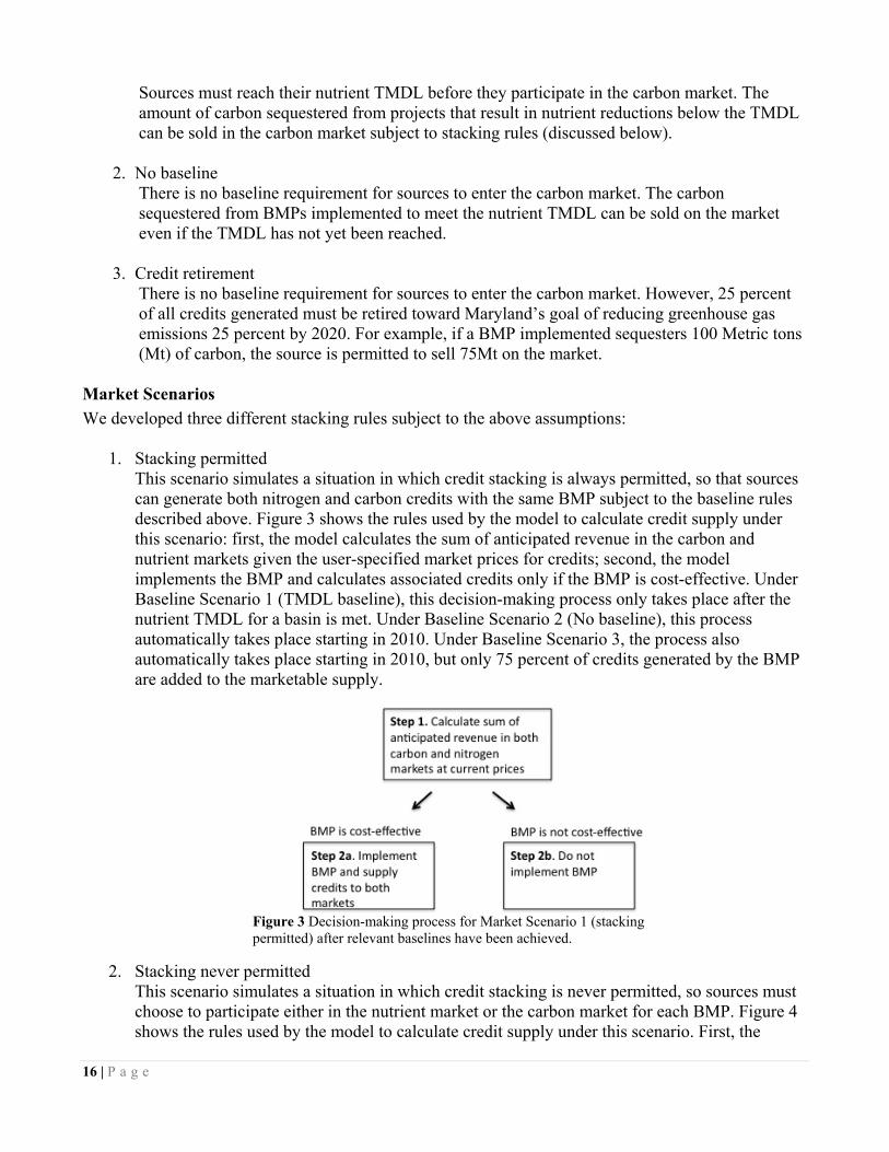
Market Scenarios We developed three different stacking rules subject to the above assumptions:

1. Stacking permitted This scenario simulates a situation in which credit stacking is always permitted, so that sources can generate both nitrogen and carbon credits with the same BMP subject to the baseline rules described above. Figure 3 shows the rules used by the model to calculate credit supply under this scenario: first, the model calculates the sum of anticipated revenue in the carbon and nutrient markets given the user-specified market prices for credits; second, the model implements the BMP and calculates associated credits only if the BMP is cost-effective. Under Baseline Scenario 1 (TMDL baseline), this decision-making process only takes place after the nutrient TMDL for a basin is met. Under Baseline Scenario 2 (No baseline), this process automatically takes place starting in 2010. Under Baseline Scenario 3, the process also automatically takes place starting in 2010, but only 75 percent of credits generated by the BMP are added to the marketable supply.

Figure 3 Decision-making process for Market Scenario 1 (stacking permitted) after relevant baselines have been achieved.

2. Stacking never permitted This scenario simulates a situation in which credit stacking is never permitted, so sources must choose to participate either in the nutrient market or the carbon market for each BMP. Figure 4 shows the rules used by the model to calculate credit supply under this scenario. First, the

16 | P a g e

model calculates the anticipated revenue in each market individually given the user-specified market prices for each market. If the BMP is not cost-effective in either market, it is not implemented. If it is cost-effective in only one market, it is implemented and the source participates in that market. If it is cost-effective in both markets, it is implemented and the source participates in whichever market generates greater revenue given current market prices. Again, this process only takes place once any relevant baselines have been reached.

Figure 4 Decision-making process for Market Scenario 2 (stacking not permitted) after relevant baselines have been achieved.

3. Financial additionality

This scenario simulates a situation in which a financial additionality criterion is used to determine whether carbon reductions are eligible to generate credits in the carbon market. A project is eligible under financial additionality when the cost of a BMP is not covered in either the carbon or the nutrient market. Under this circumstance, sources are permitted to stack credits by participating in both markets with the same BMP. On the other hand, if the cost of the BMP is covered in either market individually, the source may not stack credits and is only permitted to participate in a single market (Bianco 2009). For instance, an afforestation project meets the financial additionality criterion if its cost will not be recovered by participating in either market; it can therefore be used to generate credits in both the nitrogen and the carbon markets. Figure 5 shows the rules used by the model to calculate credit supply under this scenario. First, the model calculates the anticipated revenue in each market individually given the user-specified market prices for each market. If the BMP is not cost-effective in either market, it is not implemented. If it is cost-effective in only one market, it is implemented and the source participates in that market. If it is cost-effective in both markets, it is implemented and the source participates in whichever market generates greater revenue given current market prices. Again, this process only takes place once any relevant baselines have been reached.

17 | P a g e

Figure 5 Decision-making process for Market Scenario 3 (financial additionality) after relevant baselines have been achieved.

Scenario analysis We simulated the three Market Scenarios subject to the two Baseline Scenarios for a total of six unique market conditions. To determine how credit prices played a role in market supply of carbon, we ran each of the six scenarios under every possible combination of nitrogen and credit prices from $5-$50 per credit. For each scenario, we calculated the following:

• Carbon sequestered (Mt) through 2030 (annually and cumulatively) as a result of BMPs implemented

• Marketable carbon (Mt) supplied as a result of BMPs implemented • Supply curves showing quantity of carbon supplied to the market at a range of carbon credit

prices. We calculated these supply curves under a range of nutrient prices to show the interplay between carbon and nutrient supplies in a stacked market.

Results This section displays the results from the model scenario analysis described above. Two sets of results are presented: (1) expected carbon sequestration benefits from all BMPs implemented and (2) expected carbon supply to the market from all BMPs implemented given the various market rules described above.

Expected carbon benefits from water quality trading Carbon sequestration for all BMPs in the absence of a carbon baseline (Baseline Scenario 1) reached 1.01 million metric tons (Mt) of carbon per year by 2030 (Fig 6).

18 | P a g e

Figure 6 Total carbon sequestered (Metric tons – Mt) each year from all BMPs as a result of Maryland's nutrient trading policy.

These results were sensitive to the carbon sequestration potential of each BMP, ranging from 1.01 million Mt/year in 2030 at the low range to 1.78 million Mt/year on the high range. Total and cumulative carbon benefits from low, mid-point, and high sequestration estimates for BMPs are compiled in Table 3.

Table 3 Total and cumulative carbon benefits (measured in '000 Mt) under a range of low to high carbon sequestration rates for BMPs

Year Total C, low

Cum. C, low

Total C, mid

Cum. C, mid

Total C, high

Cum. C, high

2010 147 252 185 309 222 366 2015 360 1,620 488 2,137 616 2,653 2020 596 4,119 812 5,542 1,028 6,959 2025 829 7,841 1,133 10,610 1,436 13,367 2030 1,010 12,548 1,398 17,088 1,784 21,610

Marketable carbon As described in the Model Development section of this report, we analyzed three Baseline Scenarios for carbon: 1) no baseline; (2) a baseline set by the nutrient TMDL; and 3) a 25 percent banking requirement. The first scenario permits sources to generate carbon credits before reaching the nutrient TMDL. The second scenario requires sources to reach the nutrient TMDL before participating in the carbon market. The third scenario does not institute a baseline, but requires sources to retire 25 percent of the carbon credits generated from each best management plan project in line with Maryland’s statewide goal to reduce its greenhouse gas emissions 25 percent by 2020. Of the 1.01 million Mt of total carbon sequestered per year by 2030, about 23,000Mt per year was marketable by landowners in Baseline Scenario 1 (no baseline). In Baseline Scenario 2 (TMDL baseline), sources began entering the carbon market around 2023 (the year basins began reaching their

19 | P a g e

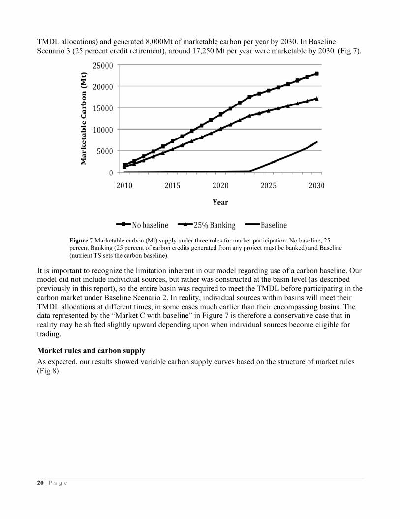
TMDL allocations) and generated 8,000Mt of marketable carbon per year by 2030. In Baseline Scenario 3 (25 percent credit retirement), around 17,250 Mt per year were marketable by 2030 (Fig 7).

Figure 7 Marketable carbon (Mt) supply under three rules for market participation: No baseline, 25 percent Banking (25 percent of carbon credits generated from any project must be banked) and Baseline (nutrient TS sets the carbon baseline).

It is important to recognize the limitation inherent in our model regarding use of a carbon baseline. Our model did not include individual sources, but rather was constructed at the basin level (as described previously in this report), so the entire basin was required to meet the TMDL before participating in the carbon market under Baseline Scenario 2. In reality, individual sources within basins will meet their TMDL allocations at different times, in some cases much earlier than their encompassing basins. The data represented by the “Market C with baseline” in Figure 7 is therefore a conservative case that in reality may be shifted slightly upward depending upon when individual sources become eligible for trading.

Market rules and carbon supply As expected, our results showed variable carbon supply curves based on the structure of market rules (Fig 8).

20 | P a g e

Figure 8 Relative carbon supply curves showing the relationship between price of carbon, P(C), and quantity of carbon supplied in the market, Q(C), subject to three different market additionality rules: S1 = Market Scenario 1 (Stacking), S2= Market Scenario 2 (No Stacking), S3 = Market Scenario 3 (Financial Additionality). Panel (a) shows supply under low nitrogen prices ($5-10/lb N) and panel (b) shows supply under mid-range nitrogen prices ($15-20/lb N).

When credit stacking was always allowed (Market Scenario 1), carbon supply was relatively inelastic, which means that supply changed little with respect to carbon prices. This is because BMP cost was nearly always covered when projects could generate credits in both markets. Since most projects generated carbon supply even when credits prices were low, credit supply remains relatively stable as prices rose. In contrast, when stacking was never permitted (Market Scenario 2), sources only participated in the carbon market when they anticipated generating greater revenue from credit sale in the carbon market than in the nutrient market. At low nutrient prices, carbon supply was much more sensitive to price (i.e. elastic) than it was when stacking was permitted. Carbon credit supply increased substantially as carbon price rose as ever more carbon projects became cost-effective in the carbon market. However, as nutrient prices rose to $15-20/lb N, most BMPs generated more revenue in the nutrient market than in the carbon market. As a result, the carbon supply curve shifted left (lower supply) and became less elastic (Fig 8). At high nutrient prices ($40-50/lb N), sources never entered the carbon market because the nutrient market always offered greater revenue, even at the highest tested carbon prices. The financial additionality criterion made it somewhat more complex to determine the interplay between carbon and nutrient prices and their combined effects on carbon credit supply. At low nitrogen prices, the carbon supply curve increased with carbon price, then “bent” backward at $25/Mt C (Fig 8). 21 | P a g e

22 | P a g e

Typical supply curves show increasing supply of a good as its price increases. The bend in the supply curve under the financial additionality criterion was explained by looking in closer detail at BMPs that were eligible for stacking. When the carbon price was less than $25/Mt, most projects met the financial additionality criterion because their cost could not be covered in either market. Carbon supply increased up until this price because higher credit prices created greater incentive to participate. Beyond this price threshold, however, fewer projects were eligible for stacking BMP costs were recovered in a single market. The decreasing carbon supply after $25/Mt shown in Figure 8 reflects the fact that fewer and fewer projects qualified for stacking as prices rose beyond this point and sources has to choose between the carbon and nutrient markets. Because most projects were more lucrative in the nutrient market, supply shifted from the carbon market to the nutrient market after stacking was no longer an option. Our results showed that in general a given marketable BMP generated more revenue in the nutrient market than in the carbon market. This is because most BMPs reduce nutrients by a greater magnitude than they sequester carbon in terms of the amounts equivalent to marketable credits. For instance, a 100-acre wetland restoration may remove hundreds of pounds of nitrogen from runoff and sequester 25 Metric tons of carbon. If the source implementing this BMP has met its TMDL, it is thus faced with the prospect of selling 10 times or more as many credits in the nutrient market than in the carbon market. Our analysis showed that when stacking credits was prohibited, carbon prices had to reach nearly eight times as high as nutrient prices to provide landowners an incentive to participate in the carbon market (Table 4).

Table 4 Break-even prices for nitrogen (N) and carbon (C) when stacking is not permitted.

BMP N ($/lb) C($/Mt) Forest buffer 5 40 Grass buffer 3 18 Wetland restoration 18 >50

Capturing true project costs Calculating true BMP project costs to the landowner is a complex issue in at least three respects: (1) the costs of land use changes (e.g. conservation buffers) are often highly variable from one BMP project to another; (2) in addition to installation and maintenance costs for land use changes, there are associated land rental costs and transaction costs; and (3) it is unclear if and how cost-sharing will affect eligibility for market participation in a market with multiple ecosystem services. The costs of land use BMPs including installation of conservation buffers and wetland restoration vary depending on the methods used to create and maintain them. Deer and other organisms that feed on plants may pose a greater nuisance to forest buffers in some regions than others, requiring more frequent chemical application or installation of protective shelters. Cost estimates for forest buffers in Maryland range from $218-$729 per acre. Likewise, wetland costs vary depending upon the extent of soil movement necessary to restore or create a viable ecosystem. Although averages around $300-400/acre have been calculated, costs for a given wetland project can reach tens of thousands of dollars (Wieland et al. 2009).

We included the variability in costs of these BMPs by using a mean cost (Table 6) and imposing a normal distribution that captured the cost variation reflected in the literature. While our method included standard costs discussed in the BMP description of this report, it did not address the potentially high transaction costs associated with assessment of projects, nor did it account for cost-sharing. While we assume that landowners bear the full cost of BMP implementation, Maryland employs several cost sharing programs to help ameliorate the financial burden of these projects for landowners, including the Maryland Agricultural Water Quality Cost Share (MACS) program and the Conservation Reserve Enhancement Program (CREP). The real cost incurred by the landowner taking cost-sharing into account will affect the credit price in the market required to provide incentives for participation, and thus the level of carbon supply. Cost-sharing may also eliminate projects from generating credits, depending on the rules of the specific market. Neither CREP nor MACs currently restricts landowners who use these funds from entering credit markets. The USDA considers revenue gained from entrance into environmental credit markets to be the property of the landowner, regardless of whether federal cost share money was used, and this approach is shared by several states that have water quality trading programs8. Maryland may choose to adopt this approach or may use conversion ratios to determine the amount of credits a landowner can sell based on their “ownership” of the BMP. We found that break-even prices ranged from $3-6/lb N to $9-12lb/N and $18-50/Mt C depending on the percentage of cost-sharing and inclusion of land rental costs (Table 5), however we did not include transaction costs or fees in these calculations.

Table 5 Break-even prices for nitrogen (N) and carbon (C) under three cost scenarios: (1) the landowner incurs the entire cost including rental payments; (2) the landowner incurs the full cost not including rental payments; and (3) 50 percent of the entire project including soil rent is covered by cost share.

Cost share BMP

Full cost w/o soil rent

Full cost w/ soil rent 50% cost-share

N ($/lb) C($/Mt) N($/lb) C($/Mt) N($/lb) C($/Mt) Forest buffer 6 40 11 >50 6 35 Grass buffer 3 18 9 44 5 25 Wetland restoration 8 >50 12 >50 8 >50

23 | P a g e

Market prices of carbon t is a result of the supply, which we have estimated here from agricultural

The price of a carbon crediBMPs in MD, and demand for credits. In the absence of a demand-side analysis of carbon credits, it isnot possible to predict whether or when prices might reach the high levels necessary to provide sourceswith the incentive to participate in carbon markets instead of nutrient markets when stacking is not permitted. Historically, prices in formal markets including the Regional Greenhouse Gas Initiative

8 For more information on water and carbon markets in other Chesapeake Bay states, see the companion paper to this document: Selman and Friedman (2010) An Overview of Water Quality and Carbon Markets in the Chesapeake Bay. World Resources Institute: Washington, DC.

24 | P a g e

t

he-

ly

he market price of credits will depend in large part on the structure and organization of Maryland’s

n

t

Conclusion ient trading program has the potential to provide environmental benefits, both in terms

ve

nother important step following this report is quantification of carbon demand. This analysis revealed

nal.

References ) Fact Sheet: Stacking Payments for Ecosystem Services. Word Resources Institute:

ostanza, R. et al. (1997) The value of the world’s ecosystem services and natural capital. Nature 387:

e Groot, R., M. Wilson and R. Boumans. (2002) A typology for the classification, description and valuation of ecosystem functions, goods and services. Ecological Economics 41: 393-408.

(RGGI) and the Chicago Climate Exchange (CCX) are far lower than the break-even prices revealedthrough our analysis. Carbon dioxide prices in RGGI have remained below $4/allowance since the firsauction in September 2008 with an average price of $2.67/allowance over eight auctions between September 2008 and June 20109. Prices in the CCX market remained below $8/allowance since January 2004, averaging $4.43/allowance between 2004 and 201010. Still, the non-binding over-tcounter (OTC) market has involved carbon credit sales as high as $300/metric ton (Hamilton et al. 2009). Though rare, these transactions provide evidence that some buyers are willing to pay relativehigh prices for credits. Tnutrient trading with carbon benefits policy and any future federal policies on ecosystem markets. Forexample, the following considerations could influence the level of demand: (1) change of the current TMDL when the federal TMDL is issued; (2) the choice or ability of buyers and sellers to participate iregional markets (RGGI) versus national or international markets; (3) the level of monitoring and oversight associated with implementation of BMPs; (4) changes in scientific information regarding carbon sequestration potential of BMPs; (5) changes in technology that improve nutrient loading or carbon capture and storage; and (6) land use and/or production changes that alter the level of nutrienloading.

Maryland’s nutrof air and water quality, irrespective of multiple market opportunities. In most cases, the presence of the nutrient market alone will provide sufficient incentive for sources to implement BMPs even after they have reached their TMDL. Only in cases where sources expect to obtain prices 5-8 times higher will they choose to enter the carbon market instead of the nutrient market. A financial additionality criterion may provide additional incentive for BMPs that are not cost-effective in either a carbon or nutrient market. However, future research should investigate whether this criterion will carry excessitransaction costs associated with measurement and monitoring. Athat quite high carbon prices are necessary for sources to choose the carbon market instead of the nutrient market. It is not possible to predict whether these price differentials are realistic to expect without an understanding of the magnitude of demand in potential markets, both regional and natioFuture research that examines demand levels under various conditions could provide additional insight into the feasibility of markets for multiple ecosystem services.

Bianco, N. (2009Washington, DC. C253-260. d

9 Data from RGGI auction results made available on the RGGI website (www.RGGI.org) 10 Data from CCX historical price trends made available on the CCX website (www.chicagoclimatex.com)

25 | P a g e

e oluntary Carbon Markets. A report by Ecosystem Marketplace and New Carbon Finance: 20 May

J., M. Mazzotta and T. Patterson. (2009) Toward a rational exuberance for ecosystem services arkets. Journal of Forestry: 204-212.

Adopts a Riparian Buffer – Benefits and Costs. Maryland ooperative Extension Service Fact Sheet 774.

Ecosystem Services: Principles, Objectives, Designs, nd Dilemmas. World Resources Institute: Washington, DC.

limate Action Plan. Maryland epartment of the Environment.

007) Cover Crop Practices Definitions and Nutrient and Sediment eduction Efficiencies, for use in the Chesapeake Bay Model Phase 5.0

r Technical Bulletin No. (TB-909) 69 pp, April 2004.

. Gans, and A. Martin. (2009) Costs and Cost Efficiencies for Some Best anagement Practices in Maryland. NOAA/DNR: Silver Spring, MD.

Hamilton, K., M. Sjardin, A. Shapiro and T. Marcello. Fortifying the Foundation: State of thV2009. Kline, m Lynch, L. (undated) When a LandownerC Marhsall, L. and M. Selman. (2010) Markets fora Maryland Commission on Climate Change. (2008) Maryland CD Simpson, T. and S. Weammert. (2R USDA. Economics of Sequestering Carbon in the U.S. Agricultural Secto1 Wieland, R., D. Parker, WM

26 | P a g e

Appendices 

Appendix A. Markets for Ecosystem Services: Principles, Objectives, Designs, and Dilemmas Prepared by Liz Marshall & Mindy Selman, World Resources Institute

A.1 Background and Introduction

In the policy debate over how to halt or reverse degradation of the world’s ecosystems services, markets are increasingly explored as a tool for attracting increased public and private investment into conservation efforts. Offset markets for ecosystem services can also help distribute the costs of compliance in ways that reduce the aggregate costs of environmental regulation. The same characteristics of ecosystems services that have made it difficult to ensure their protection in the past, however, poorly defined property rights, measurement uncertainty, and difficulties assigning value and identifying beneficiaries, make the establishment of markets in these areas challenging. Furthermore, the existence of multiple markets that are not well coordinated may actually undermine the environmental effectiveness of one or more markets if the integrity of the “additionality” criteria for offset generation is not maintained. In this report we explain the implications of individual market design for environmental objectives as well as how such environmental objectives factor into planning appropriate interactions among markets when multiple markets exist. What are Ecosystem Services? The Millenium Ecosystem Assessment defines ecosystem services as the benefits that people obtain from ecosystems (Figure A1; MEA 2005). The assessment further defines four categories of services:

• Provisioning services (or ecosystem “goods”) such as food, fresh water, fiber and fuel; • Regulation services (or ecosystem “outcomes”) such as the biophysical processes that control

climate, floods, diseases, air and water quality, pollination, and erosion; • Cultural services (or ecosystem “benefits”) such as the recreational, aesthetic, or spiritual

benefits produced by an ecosystem; and • Supporting services (or ecosystem “functions”), or the underlying ecosystem processes such as

formation of soil, photosynthesis, and nutrient cycling. This definition broadly encompasses several aspects of ecosystem function. Other definitions limit ecosystem services to include the first category listed above, or those components of nature that are directly consumed to yield human well-being (Boyd and Banzhaf 2006). In sculpting the landscapes in which we live and providing for our welfare, modern societies have largely focused on enhancing our capacity to provide the first of these categories. Manipulation of provisioning services has been a key tool in the search for increased welfare because their connection to welfare is so immediate and tangible—everybody needs to be housed, clothed, and fed. The formal and informal institutions that influence land-use decision-making, and the land-use decisions and production practices arising in response, have sought to optimize management for this subset of the total services provided by the natural landscape.

27 | P a g e

Figure A. 1 MEA categorization of ecosystem services.

We have failed to design landscapes, or the institutions that influence them, around the remaining services that intact ecosystems provide in part because we did not recognize the importance of those other services to human welfare. The other categories of services were easy to overlook; even when neglected in the development of institutions and production and consumption patterns, increasingly fragmented and degraded ecosystems continued to provide regulating, supporting, cultural, and preserving services. But such systems are not infinitely resilient, and as pollinator populations collapse and shrinking forested carbon pools release large quantities of GHGs into the atmosphere, awareness is increasing about the importance of these hidden services, their vulnerability to traditional patterns of development and decision-making on the landscape, and the potential for catastrophic welfare impacts from their loss. The premise underlying the concept of ecosystems services—that human welfare depends on the goods and services provided by healthy ecosystems—can be traced back as far as Aristotle (Ruhl and Salzman 2007). The language of ecosystem services, however, was born more recently of an effort to convey the importance of ecosystem health for human welfare beyond the boundaries of the scientific community. A few seminal publications represent milestones in the effort to broaden awareness of ecosystem services:

• Nature’s Services, by Gretchen Daly, a book which described ecosystem services in laymen’s terms and made a preliminary attempt to assess their monetary value;

• “The Value of the World’s Ecosystem Services and Natural Capital” (Costanza 1997), a controversial study reported in the journal Nature that attempted to put a global on ecosystem services; and

• The Millennium Ecosystem Assessment, which represented the first comprehensive attempt to assess the health of the world’s ecosystems, and found that, of the 24 assessed, 15 are in serious states of decline (MEA 2005).

These publications introduced, respectively, the vocabulary, the media attention, and the scientific rigor required to propel the concepts of ecosystem services, and services valuation, toward the mainstream.

Proponents of an ecosystem services approach to conservation argue that focusing attention on economic values and anthropocentric reasons for ecosystem preservation, rather than on the intrinsic or aesthetic values of nature, facilitates the involvement of a wider array of stakeholders and a broader repertoire of tools and incentives in preservation efforts (Reid 2006; Michelle Marvier et al. 2006). For instance, identifying a discrete group of people who benefits from a particular ecosystem service or good, as well as another discrete group of people who has control over the condition of that service or good, creates the potential for negotiation between those parties to result in improved condition and increased provision of ecosystem services. Such negotiations often involve incentives and transfers called payments for ecosystem services (PES). Payments for Ecosystem Services The PES approach to environmental management is straightforward: pay individuals or communities to behave in ways that increase levels of desired ecosystem services (Jack et al. 2008). Sven (2007) proposes the following formal definition of a PES scheme: “A voluntary transaction in which a well-defined environmental service (or a land-use likely to secure that scheme) is bought by a (minimum of one) buyer from a (minimum of one) provider if and only if the provider continuously secures the provision of the service.” This definition is broad enough that many of the traditional conservation programs in the United States qualify as PES schemes characterized by a government buyer acting on behalf of the public good. Such programs include the Conservation Reserve Program, a voluntary land retirement program, and the Environmental Quality Incentives Program, in which government cost-share dollars are allocated to farmers for adoption of more sustainable crop production and manure management practices.

Figure A. 2 PES refer to a suite of incentive-based mechanisms that operate within a broader framework of environmental policy instruments. (Source: Jack et al. 2008).

Many proponents of an ecosystems services approach to conservation, however, highlight the potential to create “markets” that bring together private buyers and sellers to negotiate trades in environmental services. Markets for carbon sequestration services, for instance, have developed rapidly in the wake of climate legislation and regulation both regionally in the United States and in the E.U. This publication focuses on the promise, potential, and issues associated with developing markets for ecosystems services. The discussion will at times address issues or limitations that are specific to market 28 | P a g e

development, and at other times discuss issues that are more broadly relevant to PES schemes in general, but it is important to continue to recognize the distinction between the two. While markets and PES schemes are frequently, and mistakenly, equated to one another, in fact markets are only one platform for negotiating provision of services through PES payments.

A2. Markets for Ecosystem Services

“If the provision of ecosystem services  is clearly valuable, then why don’t more payment schemes exist? Why are markets so hard  to set up? The answer  is  threefold:  ignorance, institutional inadequacy, and the problems inherent in public goods.” – Salzman, 2005 

Paquin and Mayrand (2005) cite several drivers for the acceleration of interest in markets for ecosystem services (MES) in the last decade. The first is a general shift away from command-and-control policies toward market-based instruments in environmental protection. The second is an increased capacity to place a value on ecosystem goods and services (EG&S), and the third is rising demand for ecosystem goods and services among public authorities, private entities, and consumers. A number of inventories review existing efforts to establish markets for ecosystems services worldwide (Pagiola et al. 2002; Mayrand et al. 2005; Selman et al. 2009). Existing markets have a variety of structures that are often highly customized for their particular context (Paquin et al. 2005); the complexity of the task of developing a market makes it difficult for a single market structure to emerge as a model. A simple definition of a market is “a mechanism that allocates and re-allocates resources between traders” (Gustafsson 1998). The resulting distribution of resources reflects the outcome of voluntary trades driven by the needs and interests of the market agents. Generally market transactions involve a structure in which either the sellers or the buyers compete for the purchase or provision of a commodity; one party approaching another party to negotiate provision of an item is a transaction that occurs without need of a “market” per se. An ecosystem services market is therefore an institution that enables transactions between parties who have an interest in purchasing ecosystem services (or the improved condition of ecosystem services through the purchase of related commodities) and other parties who have control over condition of ecosystem services that allows them to supply improved condition if sufficient incentive is provided. The simplicity of the definition above masks the complexity of the task when applied to ecosystem services. Consider that there are several required components to the market described above, including, but not limited to:

• A well-defined unit of ecosystem service that is to be traded and some methodology for reliably and robustly measuring how many units are created by any given supply action (an identifiable good);

• Well-defined property rights for the ecosystem service that allow ownership to be transferred, if applicable, or allow suppliers to make credible long-term contracts related to supply (a tradeable good);

• A party with a motivation to provide payment in exchange for improved ecosystem service (demand for a good);

• A party with sufficient motivation to supply ecosystem services; • The necessary institutional framework—a set of protocols for payment, contract design and

long-term monitoring and enforcement of the supply contract; and 29 | P a g e

30 | P a g e

• Transaction costs in bringing together buyers and sellers that are not prohibitively high. Creating markets for ecosystems services has the potential to harness additional resources and involve more stakeholders in conservation efforts. However, a thorough evaluation of the role of each of these components is required in order to understand the likely behavior of markets and to design markets that achieve the objectives that society establishes for them. In this paper we will focus on the first four of market criteria listed above. Defining Units of Ecosystem Services The first step in defining a unit of trade is to be able to measure discrete units of ecosystem services that will act as a transferable commodity. It is simple to walk into a grocery store and pluck a jar of pickles or a bag of chips off a shelf. You can be more or less certain that you will leave the store with the specified weight in pickles and half a bag of chips packed into a lot of air. But if there were an Ecosystem Services counter in the grocery store that I could walk up to and say “I’d like cleaner air” or “I’d like improved ecosystem resilience through balanced biodiversity,” it is a lot less clear what the ecologist behind the counter could give me to make me feel that I had in fact purchased clean air or increased resilience. In many ecosystem markets, the commodity traded is a proxy for the service desired; if I want cleaner air, I pay for a reduction in dirty air by contracting for reduced emissions. Identifying relevant units for such transactions is easier in some markets (carbon and nutrient trading markets) than in others (biodiversity markets). Because ecosystem services cannot be decoupled from the land that supports the systems that provide services, often the tradable proxy that is settled on is a unit of land or acreage so that the ecosystem services is represented in the marketplace by acreage that is presumed to provide that service. Once trading units have been identified, measuring them, and their response to changes in supplier behavior, is easier in some contexts (i.e., point-source air and water emissions) than in others (non-point-source air and water emissions). In the carbon market, for instance, it is much easier to measure the emissions impact of installing CO2 scrubbers on a smokestack than it is to measure the emissions impact of changing cropping practices from conventional to no-till in order to sequester more carbon in the soil. Soil responses to tillage changes are a complex function of tillage history, soil type, climate, crops grown, etc., and soil carbon measurements vary from one point in a field to another. Developing standard accounting protocols for the emissions reduction effectiveness of no-till is therefore extremely difficult, yet such protocols are an important part of defining the emissions reduction “supply” associated with a change in farmer behavior. These measurement problems are one of the reasons that traditional command and control regulation has focused on point source pollution; pinpointing causality within agriculture and other non-point pollution sources is difficult, and quantifying the effectiveness of mitigating best management practices is equally difficult. Continued development of and investment in scientifically credible measurement and accounting systems for ecosystems services will therefore be critical to the successful development of ecosystem services markets and other “payment for performance” incentive programs. Property Rights and Ecosystem Services The decline of ecosystem health worldwide has been blamed in part on the failure of institutions to adequately recognize and protect the values generated by natural systems (Cork 2002). This failure includes the more widely recognized “market failure,” where economic markets fail to internalize the

31 | P a g e

external costs of environmental impacts associated with market transactions. More fundamentally with respect to ecosystems services, however, institutional failure includes a failure to establish formal rules of access to, and ownership of, ecosystem goods and services, as well as to develop an understanding of how those rules interact with more generally recognized rules of land ownership. It is an age-old tenet of economics that when rules of ownership are unclear, so too are the rights and responsibilities for maintaining those services (Cork 2002). For ecosystem services to be suitable for market development, some proxy representing that service must be both measurable (as described above) and transferrable as an economic good. In order to be transferrable, a good must have property rights defined for it that confer upon the holder of that right three fundamental components of ownership:

1. The exclusive right to control use of the good; 2. The right to earn income from the good; 3. The right to transfer ownership of the good to others.

There are two major obstacles to establishment of well-defined property rights for ecosystem services. One is a lack of understanding or consensus about who owns these services in the first place-- the initial distribution of use rights and who has the right to trade those benefits. The other obstacle arises from the characteristic of ecosystems services themselves; defining a property right as described above can be very difficult for goods that have “public goods” characteristics. To understand the difficulties of assigning property rights to ecosystem services with public goods characteristics, consider first the ease with which we assign a property right to a commonly transferred good like an apple. An apple has a set of characteristics that facilitate using a market mechanism to ensure that apples are produced in sufficient supply and distributed to their highest valued use. In this context, the most important of these characteristics are excludability and rivalry. Excludability means that it is possible to exclude somebody from consumption of the good if they refuse to pay for it. In the case of the apple, excludability is clear; if you don’t pay for the apple, you don’t get the apple, and you can’t eat the apple. Rivalry means that consumers are rivals in their consumption of the good; if one consumer consumes a portion of the good, that portion is no longer available for consumption by another. Again, with the apple, rivalry is clear; if you eat the apple, it is no longer available for consumption by another. Markets are excellent at ensuring that apples are produced in sufficient supply and distributed to their highest valued use purely through the action of individual consumers’ market transactions; if you want to consume an apple, you have to pay for it, and you do not benefit from apples that others have consumed, so you have to pay for your own. The individual’s demand therefore reflects the value that the individual places on the apple, and the market is efficient at arriving at a price that reflects the value of the apple and at inducing farmers to participate in the market by supplying apples at that price. The failure of markets to ensure a sufficient supply of ecosystem services, on the other hand, is often attributed to the fact that the benefits from ecosystem services have characteristics of “public goods,” meaning that they are non-rival and/or non-excludable. Consider the climate stabilization service provided by a large expanse of intact forest. If that forest is threatened, and somebody concerned about climate steps in to pay to protect it, the benefits of that transaction are neither rival nor excludable. Even if I don’t donate to help cover the costs of protection, nobody can stop me from enjoying the benefits of a more stable climate (hence the non-excludability). Similarly, the fact that my neighbor is also enjoying those benefits in no way detracts from the benefit that I gain (hence the non-rivalry).

32 | P a g e

The problem when using markets to ensure ecosystem health is that when goods have public goods characteristics, many people will refrain from participating in the market in the hopes that someone else will provide payment for the good, thereby allowing everyone to benefit. Why pay for it if someone else might pay for it and you can get it for free? Such “free riders” distort the market because the market transactions do not reflect the value that all individuals place on the good. The market implications of this distortion are significant: demand does not capture the full social value, the market price is lower than optimal, and the amount of ecosystem services supplied through market transactions is lower than optimal. The “real world” implications of the distortion are equally significant: degraded air and water quality; failing pollination services; unstable climate patterns; and the list goes on. To compensate for such market failures, governments have traditionally played a significant role in the provision of public goods. The government, acting on behalf of the public, attempts to satisfy social demand for goods through a range of public programs designed to increase supply of that good. Examples of sectors where the government has stepped in to ensure appropriate provision of services in the name of public welfare include public education, national defense, and government conservation programs aimed at reducing erosion and controlling degradation of soil and water quality from agricultural production. Transferring some responsibility for ecosystem services provision out of the hands of governments and back into markets requires that you somehow address the characteristics of public goods that created market failure, and government intervention, in the first place. Increasingly, correcting for market failure in the provision of ecosystem services involves creating demand for ecosystem services through regulation. One way to circumvent the public goods nature of ecosystem services transactions is to “privatize” either supply or demand. Supply can be privatized by restricting access to a resource (i.e., creating an excludable resource from a resource that has traditionally been considered “common property”, such as the right to a specified level of catch within a fishery). Demand can be privatized by creating regulatory incentives for certain individuals to demand the resource, thereby forcing the good to be a rival good in the sense that certain parties are responsible for a certain amount of mitigation that they cannot rely on others to provide. Clearly, there are several important categories of questions related to the definition of property rights that must be resolved for successful establishment of a market in ecosystem services. Questions related to supply include, who has the right to claim ownership of ecosystem services and their proxy and how does that influence appropriate management of resources? Questions related to demand center around the question of how to correct for market failures related to public goods characteristics of ecosystem services and reduced incentives to participate in the market.

6. Institutions that allow for an equitable redistribution of resources (i.e., pro‐poor ESM mechanisms). 

5. Institutions  that  provide  an  incentive  for  ancillary  preservation  of  non‐valued ecosystem services (assuming that services are co‐produced by ecosystems) 

4. Institutions that  improve the viability of farms and farming and assist farmers  in the support of other social objectives such as food objectives. 

3. Institutions  that  maintain  the  “integrity”  of  landowners’  property  rights  by ensuring that they receive compensation for the value of ecosystem services that they manage for the public good. 

2. Institutions that will spread the compliance costs for environmental regulation in a way that minimizes the total cost of meeting environmental objectives. 

1. Institutions that will harness additional resources and involve more stakeholders in conserving ecosystems and sustaining the services they provide. 

In  the context of ecosystem services, many of  these preconditions do not yet exist, so building a market means building from scratch. Given these difficulties, where does the enthusiasm for markets come from? What do proponents believe that markets will help us achieve with respect to environmental and resources conservation objectives. 

 Objectives for Ecosystem Services Markets 

Demand for Ecosystem Services Although proponents have many objectives for the creation of ESM mechanisms (see text box), one of the most commonly cited reasons is to help achieve environmental and resource conservation objectives. The argument is that markets can help us get increased provision of improved ecosystems services. But, as mentioned above, the public goods nature of ecosystems services distorts markets by creating the possibility of “free riding” on the benefits generated when others participate in a market place. What types of measures can be introduced to motivate a buyer to seek improved ecosystems services through a marketplace, and what are the implications of such measures for aggregate improvement in environmental condition? The driver for demand in most existing ecosystem services markets is government regulation (Salzman 2005). Government regulation, for instance, identifies a discrete set of parties to hold responsible for reductions in some activity or emission with negative impacts on ecosystem services. An example of such a regulation is a regulatory “cap,” where the government determines the maximum allowable level of an activity, and then uses some mechanism to distribute that allowable activity among firms. The firm must then choose a set of activities to correct for the difference between their actual level of emissions and their allowed level of emissions. If a market exists, the regulated party then has the option of either meeting the regulation through their own reduction, or turning to the market to purchase the reduction (in the form of a credit) from somebody else. Such markets, which would not exist in the absence of regulation, are called “regulatory markets” (Hirsch 2007). The primary driver for the rapid growth in water quality markets recently has been the implementation or forthcoming implementation of nutrient caps that limit nutrient pollution discharges (Selman et al. 2009). There are two fundamentally different types of credits that can be traded in regulatory markets, depending on the type of credit supplier. The seller may also be a regulated party and subject to the

33 | P a g e

34 | P a g e

cap, but capable of reducing their emissions at much lower cost than the buyer and therefore willing to accept some payment in return for reductions beyond what they are required under regulation to provide. Such markets, where regulated parties sell off their “allowances”—or units of what they are allowed to emit under the regulation—in exchange for compensation, are called allowance markets. Allowance markets distribute the reductions required by regulation to those regulated parties who can provide them at least-cost, so that the costs of compliance are minimized within the regulated sector. A different type of credit is created when sellers from unregulated sectors are allowed to sell reductions. Unregulated sectors are sectors that do not fall under the cap and are therefore not required to reduce their emissions. Such sectors, however, may be capable of reducing emissions at lower cost than the regulated sectors. Reductions created by unregulated parties are called “offsets” and, if allowed in a particular market, can be sold to regulated parties to “offset” emissions within the regulated sector. Note that in both cases, whether allowances are traded or offsets are traded, the total reduction achieved is determined by the regulation. When only allowances can be sold, the regulated reduction is fully achieved by parties within the regulated sector. When offsets can be sold as well, the regulated number of reductions is achieved, but those reductions are split between the regulated sector and another unregulated sector that voluntarily reduces emissions in exchange for payments. Under the offset scenario, the regulated sector emits more than it would if only allowances can be sold. The take-away message is that when markets for ecosystem goods and services are regulation-driven, buyers do not participate in those markets in order to improve the condition of the environment; they participate in EG&S markets in order to achieve required environmental objectives at lower cost. When offset markets exist, it is tempting to point to the fact that an unregulated sector is voluntarily making improvements as a way of supporting the argument that the market is providing an incentive for additional improvements to environmental or ecosystem health. In fact, however, those improvements merely compensate for the fact that regulated sectors are not making required improvements elsewhere. Improvements in the unregulated sector that are used to generate tradable offsets for ecosystem goods and services are therefore not “additional” in the sense that aggregate provision of ecosystem services increases in the presence of the market. Therefore, enabling trade through a market in ecosystem services distributes and reduces aggregate cost of compliance with a regulation, but it does not, in and of itself, achieve aggregate environmental improvements that would not exist without the market. Markets will not automatically provide incentive for environmental improvements beyond that required by the regulation; in the absence of the market the regulation would still ensure that environmental objectives are met, but at higher aggregate cost. Markets that aspire to create additional incentives for ecosystem improvement must specifically build in market design features that ensure an increase in aggregate ecosystem improvement beyond what is required by the regulation that drives the market demand. There are, in addition to regulation obligations, other private sector motivations for participation in a MES, including bottom-line considerations, marketing strategies, corporate social responsibility policies, or an effort to seize new market niches (Paquin and Mayrand 2005). To be able to make environmental benefits claims about participation in MESs, however, such firms must ensure that markets are designed with environmental benefits, not just cost-reduction, in mind.

A3. Ecosystem Services Markets and Environmental Improvement If the achievement of additional environmental improvement is an explicit objective in the establishment of markets, specific design features must be incorporated into the market to ensure that such additional benefits are achieved. A variety of mechanisms have been proposed to do just that: baseline practice and/or performance requirements for ecosystem service suppliers in offset markets; retirement ratios altering the proportion of credits demanded to credits supplied; requirements related to ancillary, non-valued ecosystems services, etc.

“Setting the baseline is one of the most critical aspects of project design because it defines the additional carbon that will be sequestered as a result of the project.” – Murray et al.  2007 

The selection of an appropriate baseline has been a flashpoint in the design of water quality trading markets for years. Selecting a baseline in this context refers to establishment of a set of practice and/or performance requirements that a provider of an ecosystem service must satisfy before additional improvements can qualify as offset credits to be sold on an ES market. Baselines ensure that certain standards of landowner behavior with respect to environmental protection are met before additional changes in behavior can be rewarded through the marketplace. Baselines can be set at current practice; such baselines ensure that establishment of a market does not offer the perverse incentive for landowners to first “dirty” up their behavior in order to be compensated for later clean-up under the market structure. Alternatively, baselines could be set assuming that it is reasonable to expect some level of best management practice from landowners. Although regulations requiring best management practices, or some minimum provision of services, don’t exist for most landowners, this approach makes entrance into the potentially lucrative credit markets contingent on first achieving a specified set of minimum standards. By failing to reward people for changing behavior that was considered “sub-standard” in the first place, such baselines imply that landowners share some responsibility for the protection and provision of ecosystem services and that the government therefore has a right to regulate “up to a certain point” (Jones et al. 2009). There is a spirited debate around the question of where to draw the line in determining a baseline, however. How much are farmers responsible for protection of the ecosystem services provided on their land versus how much freedom do they have to use their land in ways that could compromise those services? This decision will determine how effective the market is at inducing non-regulated sectors in offset markets to make additional improvements, though setting baseline performance requirements too high could create a barrier to market entrance that prevents offset transactions from happening at all, in which case no additional improvements would materialize. Baselines are fundamentally important in determining the magnitude of “additional” ecosystem benefits that can be expected from establishment of a market. Any ecosystem service improvements that occur between current practice and achievement of the minimum standards for market participation are “additional improvements” attributable to existence of the market, and, more specifically, attributable to the baseline requirements imposed by that market. The larger the distance between current practice and baseline expectations, the more effective the market can potentially be at incentivizing ecosystem health benefits above and beyond those already required by the regulation driving demand in the market. Any improvements above baseline, on the other hand, are offset improvements that don’t constitute additional, market-induced improvements, but are in fact required

35 | P a g e

36 | P a g e

by the original driving regulation and therefore expected to be achieved with or without an offset market. An alternate method of ensuring net market-induced environmental benefits is to apply a retirement ratio to all trades occurring within a market. Retirement ratios require that a proportion of credits supplied be retired with each trade rather than being applied toward the number of credits demanded. Such ratios, also called “environmental benefit ratios” ensure that improvements are achieved beyond those required by regulation alone (Selman et al. 2009) and can be applied to offset credit trades, allowance credit trades, or both. The Maryland water quality trading program, for instance, applies a 10 percent retirement ratio to point-to-point and point-to-nonpoint trades. This requirement ensures that 10 percent of all credits generated are retired rather than being used to satisfy regulated reductions; such credits are additional to the regulation and the benefits derived can be attributed to establishment of the market. An alternative way in which ecosystem services markets have been touted as providing incentive for additional environmental improvement is through the provision of “ancillary” benefits, or the positive side effects on non-valued ecosystem services associated with changing behavior to improve supply of the valued, or marketed, ecosystem service. This argument assumes that behavioral changes in response to a single market will co-produce beneficial impacts across multiple ecosystem services. This assumption may be true in many scenarios; changing tillage practices to preserve soil productivity through reduced erosion, for instance, may also improve the nutrient cycling capacity of a plot of farmland. However, there are also cases where managing for one ecosystem service could create tradeoffs with another ecosystem service; there is potential, for instance, for changes in rotation length to maximize carbon sequestration in forests to have detrimental impacts on wildlife that rely on certain stages of tree growth. Furthermore, a failure to consider those ancillary services explicitly could mean that opportunities for extremely low-cost provision of secondary services are missed. A wetland designed or protected to facilitate nutrient cycling in response to a nutrient trading market, for instance, may fail to consider significant habitat or flood control services that could be offered if such services are accompanied by no increased nutrient benefits. At worst, the risk arises that the optimization employed in managing for a single service could undermine the integrity of an ecosystem by failing to recognize the interdependencies among services and the full value of the diverse bundle provided jointly. Ecosystem Services and Multiple Use Management The historical tendency within U.S. regulation has been to silo environmental management by establishing objectives and regulations on an issue-by-issue basis; thus we have the Endangered Species Act, the Clean Air Act, the Clean Water Act, etc. The creation of ES markets on a service-by-service basis fits nicely into this paradigm, with individual markets established to facilitate compliance with a specific regulation. Ultimately, however, the sustainability of land-use systems will depend not on the protection of individual ecosystem services but, more broadly, on the maintenance of ecosystem function necessary to provide a balanced portfolio of ecosystem services, some of which we can recognize and estimate market values for, and some of which we cannot. Ecosystems represent complex interactions among several different services, with feedbacks, thresholds, time lags, and interdependencies. Conceptual frameworks that emphasize the existence and importance of individual services, such as that introduced by the MEA, are useful as a means of illuminating the link between ecosystems and welfare but should not be interpreted as implying that ecosystem function can be effectively managed on a service-by-service basis.

37 | P a g e

Long before the explosive interest in ecosystem service markets, scientists recognized the importance of “multiple-use management” in managing ecosystems, and land-management agencies such as the USFS adopted multiple-use land management as an explicit objective as early as 1960 (Multiple Use Sustained Yield Act). The challenge, however, lies in how to apply that framework to inform decisions or drive policy and research (PNW 2008). How does one define and then design regulations to protect “balanced bundles of ecosystem services”? Is it possible to assess and measure the health of an ecosystem without disaggregating it into individual services, and, if not, how can you manage more broadly for the health of an ecosystem without falling back on management of individual services? How can ecosystem markets fit into a broader multiple-use management paradigm? One approach to the co-production of services is to develop markets for “bundled” ecosystem services rather than for individual services. Bundling means that multiple ecosystem services are traded as a single commodity in a single transaction (Jones et al. 2009). That commodity can be envisioned as a single “ecosystem services” credit, which is an index of environmental improvements along multiple dimensions, or, alternatively, as a proxy for such an index, such as acreage conserved. The latter formulation is the basis of the wetlands market—a bundled ES market whose tradable “ecosystems services” unit is an acre. Bundled markets may better reflect that ecological systems are complex networks that may more successfully be managed as a system rather than on a component-by-component basis. If a single project receives payments from multiple programs for multiple services that it generates, on the other hand, those payments are said to be “stacked.” Allowing landowners the flexibility to receive stacked payments from multiple markets has been advocated by some because of the increased incentive that it will provide for landowners to participate as suppliers in ecosystem services market. Others, however, denounce such stacked payments as “double dipping” because they represent multiple payments for the same activity (Woodward and Han 2008). Neither argument is incorrect; allowing stacked payments has both pros and cons. The key to designing appropriate ways to accommodate multiple markets will be understanding how different stacking mechanisms balance those pros and cons and what the resulting implications are for supply incentives, environmental impact, and cost-effectiveness of regulation compliance.

A4. Ecosystem Services and Multiple Markets

The proliferation of potential markets for ecosystem services raises interesting questions about how such markets can and should interact with each other and what the implications of multiple markets are for cost and conservation objectives. The potential for co-production of ecosystem services described above, for instance, means that a single project could potentially generate credits that feed into multiple markets in some way. In the United States, for instance, the most advanced markets have been developed in the areas of carbon sequestration and nutrient pollution reduction, and there are many potential best management practices on agricultural land that could produce both carbon benefits, in terms of increased sequestration, and nutrient benefits, in terms of reduced nutrient pollution. The co-production of benefits, however, complicates the translation of environmental improvements into marketable credits because it complicates standard interpretations of baselines and additionality.11

11 In some cases ecosystem markets are planned together where benefits are co-calculated and baselines are coordinated. For example, Maryland’s water quality market includes “sub-markets” for both nitrogen and phosphorus. The nitrogen and

38 | P a g e

Additionality requirements are usually attached to markets in order to ensure that conservation dollars, or conservation compliance dollars, are not spent on environmental improvements that would have occurred even without that transaction. It is difficult to cleanly apply such a criterion to products that are jointly created; if the market for carbon is driving a particular project, can one argue that nitrogen credits also created are “additional” in the nitrogen market? Those improvements may have occurred anyway, even without the nitrogen market, due to the incentives provided by the carbon market. Concerns related to defining performance baselines and ensuring additionality in the presence of multiple markets therefore raise significant issues associated with accounting for co-benefits that must be addressed in deciding an appropriate set of guidelines for how to accommodate multiple markets. Allowing stacking may expand the focus of management decisions beyond a single ecosystem services, but it may also “waste” conservation dollars on projects that would have occurred anyway. Conversely, not allowing stacking may affect market participation and the types of projects that are incentivized by the market. The latter argument in favor of stacking is straightforward: if landowners can gain increased revenue by selling into multiple markets, they are more likely to consider engaging in a wider suite of possible projects with multiple ES benefits. As argued above, such projects do not necessarily imply net additional ecosystem service benefits; if the credits are sold as offsets into those multiple markets, they simply compensate for losses elsewhere. The presence of multiple markets, however, does incentivize projects with a more balanced portfolio of ES benefits, rather than projects that focus on only a single ES benefits, which could help improve ecosystem management overall (Bianco 2009), and possibly provide a more robust set of non-valued, ancillary ES benefits. Arguments both in favor of and against stacking have merit, and the relevant question is how to ensure additionality in the presence of stacked payments. The underlying issue is how to account for those multiple benefits—how do the benefits achieved along each ES dimension translate into credits for each independent ES market? As described above, in a single market, credits are calculated as the difference between the new, project-induced benefits, and the benefits achieved under the specified baseline (with some modification for trading ratios, if required). For the first dimension along which you explore ES improvement (which we will refer to as the “primary market”), that calculation is straightforward. If you try to apply the same additionality criterion to the secondary market, however, you run into the issue of selecting the relevant baseline for the secondary market. For the purposes of illustration, imagine that the baseline in the secondary market is defined as “current practice.” In this context, does “current” refer to a scenario with or without the primary market? If “current practice” refers to a scenario with no markets in place, then all benefits generated by the project are considered above and beyond the baseline. In that case, the second ES dimension is awarded the same number of credits as it would have been in a single market scenario; the two ES markets are interpreted to be completely independent and credits are awarded as if the other market did not exist as an incentive mechanism for behavior change. Such payments are considered “fully stacked.”

phosphorus reductions from a single project are co-calculated, but each is subject to its own baseline; a landowner cannot generate and trade nitrogen and phosphorus credits unless the project meets baseline requirements for both. The additionality discussions in this paper restrict themselves to ecosystem markets that operate independently of each other and have determined baselines separately.

39 | P a g e

jointly

The problem with fully stacked payments becomes evident when you consider that the integrity of each independent ES market relies upon the assumption that all credits sold into that market are “additional” in the sense that they wouldn’t have occurred in the absence of that market. All payments for ecosystem services are designed to incentivize an environmental benefit that would not have otherwise occurred, or to prevent an environmental harm that otherwise would have occurred (Bianco 2009). It is that assumption that allows the benefits generated to serve as offsets without compromising the original environmental objectives of the regulations driving the respective markets. In the case of multiple markets, it is difficult to unequivocally argue that market A is what is incentivizing the behavior change, when returns are also received from market B, and vice versa. If, on the other hand, “current practice” is assumed to represent behavior in the absence of the secondary market, but with all other markets in place, then only benefits that are generated by projects that are not sufficiently incentivized by the combined effects of the other markets will be considered additional and capable of generating credits. If returns from a primary market are sufficient to cover the costs of the project, then benefits generated along the remaining ES dimensions cannot be considered “additional” to those ES markets according to the definition given above. The accusation of “double dipping” applies to such cases, where allowing landowners to receive payments for the other ES credits represents a windfall for the landowner but fails to provide incentive for any additional environmental benefits in the secondary ES markets. The secondary markets are, in effect, providing payment for ES that would have been provided anyway, driven by the primary market. Relative to a scenario in which the project occurs (financed by the primary ES market) but the remaining ES credits cannot be redeemed, allowing credits in those secondary markets to be sold as offsets for damaging activities elsewhere results in a decrease in the environmental effectiveness of the combined regulation and offset market, and a decrease in net environmental benefits. There are other scenarios, however, in which returns from a single market are insufficient to cover a project’s costs, and only the combined returns from multiple markets would provide sufficient incentive for a landowner to change land management or land use behavior (Figure A.3). In such cases, payments from both markets are necessary to drive project development, and credits in each market can therefore be considered “additional”. Credits in both markets can be thought of as partially subsidized by the existence of the other market, and, when competitively supplied, may act to drive down the price of credits in one or both markets.12 This market dynamic represents the natural movement of the market toward supply of ecosystem services that can be supplied at lower cost because they are supplied with other valued ecosystem services.

12 When not supplied competitively, prices in each market could be driven up to the marginal cost of abatement in the regulated industry. What are the implications of this in the case of stacked versus not stacked markets?

Figure A. 3 Financial additionality criterion. (Source: Bianco, 2009)

This criterion for additionality in the case of multiple markets is an extension of the concept of “financial additionality,” which has been widely debated as a potential market design requirement in the carbon offset arena. Tests for “financial additionality” refer to a determination of whether a project is commercially attractive enough to occur even in the absence of a carbon market rewarding it for GHG reductions (Reynolds 2008); many argue that, if so, projects should not be eligible to generate credits because credits generated are not truly additional under that scenario. It is argued that projects that have positive returns in the absence of a market should more appropriately be considered part of the baseline because, in theory, such projects should happen “anyway”. The financial additionality criterion applies in an analogous way to the context of multiple ES markets. If a project is financially viable when generating credits for a single primary ES market, then secondary ES markets would fail the financial additionality test, and credits should therefore not be considered additional in those secondary markets. While the distinction is theoretically straightforward, determining whether a project passes or fails a financial additionality test is extremely difficult and highly sensitive to the data and assumptions used in the returns calculation. Endowing an institution with the authority to make that decision for the carbon market in the U.S. has proven highly controversial, and financial additionality often no longer appears on recommended lists of mandatory market design elements (Reynolds 2008). Creating institutional capacity and authority for such a determination in each of a number of additional ES markets may entail significant transaction costs and generate comparable resistance. Graphical analysis of multiple markets and ecosystem credit supply Consider the case of a single ecosystem services market for nutrient credits. Farmers are willing to engage in projects so long as the returns from the nutrient credit market exceed the costs of the project. A schedule of such costs, and the credits generated, forms the supply curve for the nutrient credit market. Similarly, demand for nutrient credits as offsets is created through regulation. The demand curve is downward sloping, so that low-priced offset credits would be snatched up in large numbers whereas at high prices regulated sectors might choose instead to reduce their emissions through other means, so the number of offsets demanded is lower.

40 | P a g e

DemandNC Price $

SupplyNC

P*

Quantity of nutrient credits supplied

Q*

Figure A.4 illustrates the market equilibrium in the case where the only market driving the project decision is the nutrient credit market. At the price P* for offset credits, farmers will be willing to supply Q* credits. At lower prices, demand will exceed supply, which drives the price up, while at higher prices supply will exceed demand, which drives prices down, so the P*/Q* combination is the position that the market will tend toward.

Figure A. 4 Theoretical market equilibrium

Now consider that a second market exists for carbon credits, which can be jointly produced by the projects forming the supply curve for nutrient credits. If the farmer is receiving revenue for the carbon credits, the result will be a shift in the supply curve for nutrient credits; the costs of producing nutrient credits are reduced because some portion of that cost is covered by the returns from the carbon credit market (Figure A.5).

Price $ DemandNC

SupplyNC

SupplyNC w/CC

P*

Quantity of nutrient credits supplied

Q*

Figure A. 5 Supply and demand for nutrient credits 41 | P a g e

The result of the shift in costs is that farmers, given returns from the carbon credit market as well, should be willing to supply a greater number of nutrient credits at a lower cost. The new market equilibrium reflects that change (Figure A.6). Given the new cost structure, the nutrient credit market will now tend toward a price of P*** and a quantity of nutrient credits supplied of Q***.

Price $

DemandNC

SupplyNC

Q*

P*

Q**

P***

Q***

SupplyNC w/CC

Figure A. 6 Supply and demand for nutrient credits This graph illustrates the existence of another quantity threshold implicit in the new supply curve- Q**. This threshold represents the number of credits that are entirely paid for by the carbon credit market; these nutrient credits are produced in conjunction with carbon credits at no extra cost to the farmer. The existence of these “free” nutrient credits is one driver of the additionality debate when multiple markets exist. The argument is that farmers will provide those credits anyway, as a result of incentives provided by the carbon credit market, so the total payments on the “non-additional” credits (shown in grey in Figure A.7) are wasted conservation resources that could be more effectively spent on procuring actual, additional environmental improvements elsewhere (Bianco 2009).

42 | P a g e

Price $

DemandNC

SupplyNC

SupplyNC w/CC

Q***

P***

Q** Quantity of nutrient credits supplied

Figure A. 7 Supply and demand for nutrient credits with an interacting carbon redit (CC) market. c

From a landowner’s perspective, of course, these expenditures are not “wasted”; landowners consider that they are appropriate returns for the provision of something that society values—the environmental improvements associated with the nutrient credits. In evaluating this argument, however, it is critical to remember that creation and trade of nutrient credits that act as offsets does not automatically create aggregate environmental improvement; it merely reduces the cost of complying with a fixed requirement for water-quality improvement that would be achieved anyway, albeit at higher cost, if offsets were not sold. One method of ensuring that offset markets generate aggregate environmental improvement, rather than simply lowering costs of compliance, is to require landowners to achieve a predefined level of baseline performance as a prerequisite for participation in offset markets. The result of those criteria is to shift the supply curve and rotate it up; supplying a fixed number of credits costs more because baseline requirements must be me as well. The market result is that fewer offsets will be traded ( Q ), and they will receive a higher price in the market ( P ) (Figure A.8).

43 | P a g e

SupplyNC

DemandNC

44 | P a g e

The level of environmental improvement within the offset supply sector would be B + Q , with Q provided as offsets to compensate for nutrient emissions elsewhere in the capped sector and B generated as an additional environmental benefit, above and beyond the improvements required by the regulation driving offset demand. In such a scenario, the baseline requirements for market participation are what determine how much additional environmental benefit the existence of the market will incentivize. Rigorous baseline requirements will further shift the supply curve, resulting in fewer offset credits supplied (Q ), but potentially with greater additional environmental benefits ( B ). Note that, although not illustrated here, it is theoretically possible for the application of very stringent

Q*

P*

Quantity of nutrient credits supplied

Price $

SupplyNC w/BL

Q

PP

Q

SupplyNC w/BLstringent

Quantity of nutrient credits supplied

Baseline environmental benefits generated

B

Q Q

B

Figure A. 8 Supply and demand with baseline performance requirements.

baseline requirements to increase costs of participation in the market so much that nutrient credit provision ( Q ) drops enough for B to drop below B .

A5. Regulatory Approaches to Multiple Markets

Regulators responsible for defining whether and how multiple markets work together have a number of decisions to make about market structure that will reflect the relative importance placed on the cost-effectiveness of regulation compliance, the integrity of the additionality criteria, and the explicit pursuit of multiple environmental benefits beyond those provided by the primary market. The most conservative option from an additionality perspective is to restrict projects to participation in a single market. Projects meeting the additionality criteria of a primary market receive credits in those markets, but can then not receive additional credits from any secondary markets. This approach assumes that any benefits generated along the secondary dimensions would not be additional, as they were generated “anyway” and are therefore ancillary benefits of the project rather than credit-able additional benefits. In this case, the baseline for the secondary markets is assumed to include the existence of the primary markets. The disadvantage of such a system is the risk that some projects with multiple benefits will not move forward because the primary market alone could not cover the costs of project. In this system, there is no contingency for projects to demonstrate that returns from multiple markets are achievable and necessary for the project to move forward. The market design option occupying the other end of the spectrum would be a hands-off regulatory regime that allows a project to participate in however many markets it can demonstrate benefits in while satisfying the additionality criteria of each market individually. In this case, the assumed baseline in every market is a world with no project; this approach essentially ignores the question of additionality between markets. Treating the markets independently would remove the transaction costs associated with demonstrating that any “inter-market” additionality requirements are met. The disadvantage, however, is that market payments will be provided for environmental benefits that would have occurred anyway due to the presence of other markets. While an effective way to reward land owners for provision of ecosystem services, such an approach is not an efficient use of dollars for achievement of conservation objectives. An alternative option would use the financial additionality criterion to determine whether projects can participate in multiple markets (Bianco 2009). Under this scenario, landowners are permitted to sell project benefits into multiple markets, but they must demonstrate financial additionality in order to qualify to sell into secondary markets. Demonstrating financial additionality means demonstrating that the project will not be financially viability without the combined returns from multiple markets. A project that fails this test is one that is financially viable with returns from a single market; such a project is likely to likely to happen even in the absence of the additional markets, so the ancillary benefits generated are “non-additional” and should not be awarded credits in other markets. Where multiple market options exist, farmers could potentially have some flexibility in determining the best combination of markets to participate in to maximize net revenue—i.e., the highest paying combination—to try to maximize their own net revenue from the project, within the limitations set by the financial additionality criterion. Another option for coordinating markets creates a single aggregator institution that funnels demand from multiple ecosystem service markets into a single ecosystem services credit market that land-owners participate in (Figure A.9). Landowners therefore sell multiple ecosystem services to a single

45 | P a g e

aggregator institution (creating essentially a bundled ecosystem services product), which that institution then disaggregates and sells off individually or in bundles as determined by the nature of the demand.

Figure A. 9 A buyer, investment seller framework for ecosystem services (Binning 2002) Under this scenario, an “investment vehicle” is created that coordinates buyers from many areas with different motivations for investing in ecosystem services credits. The institution finances projects through the purchase of ecosystem services credits from land-owners; the value of those credit could include carbon credits, biodiversity credits, salinity credits, nutrient credits, etc., with the revenue received by farmers dependent on the market price of credits and on a determination of which generated benefits are “additional,” and therefore credit-able, and which are not. These credits are then unbundled and sold into the individual markets (i.e. to the individual buyers); a dealer within the investment institution tracks the stocks and flows of ecosystems credits and third-party accreditation, monitoring, and enforcement institutions ensure that only what is generated and determined to be additional can be sold (Binning 2002). This scenario essentially allows demand for individual ecosystem services, driven by issue-specific regulation, to interact with supply of a bundled ecosystem services product; the stock and flow of individual credits is coordinated by a central institution that acts as a trade facilitator across multiple markets. Defenders of Wildlife is experimenting with an online version of a voluntary marketplace organized across multiple ecosystem service markets.13 The “Marketplace for Nature” is a multi-credit ecosystem marketplace designed to attract new and private investment in conservation and to channel that investment into conservation projects with multi-dimensional ecosystem benefits.14 They will be piloting the program with a limited number of project sites identified in conjunction with the Willamette Partnership and the Bay Bank(Chesapeake).

13 http://www.defenders.org/programs_and_policy/biodiversity_partners/ecosystem_marketplace/mfn/index.php

46 | P a g e

14 While the project endorses rewarding farmers for multiple services, until more sophisticated guidelines for stacking and bundling of credits across markets are developed, they are currently limiting returns to a given parcel of land to only one kind of service.

Source: Defenders of Wildlife 

Goals of Marketplace for Nature  

1. Ecological  effectiveness.  Projects will  have  concrete  goals  and monitoring  to ensure  that  ecological  benefits  are  being  realized.  Principles  of  conservation biology including connectivity, the need for natural processes and habitats and species at risk will drive project planning.       

2. Multiple  values.  Priority  projects  will  address  water  quality  and  quantity, wetlands, endangered species, carbon and  important  fish and wildlife habitat. Other  services  may  include  pollinator  habitat  and  restoration  of  ecological processes like fire and flooding.    

3. Strategic  investments  at  a  landscape  scale.  The  Marketplace  will  reward investors  who  purchase  credits  from  projects  in  priority  areas,  like  those identified in the State Wildlife Action Plans.    

4. Transparent and credible. Existing markets are opaque and hard  to  track. The Marketplace  for Nature will apply, test, evaluate and refine tools  in the  initial pilot areas to ensure their efficacy and credibility. 

5. Accessible with  low  transaction  costs.  The  administration of  the Marketplace will emphasize efficiency and practicality to attract buyers and sellers. 

 

One advantage to a centralized aggregator working across markets is the ability to be more strategic in how ecosystem services are valued and how projects are financed. The aggregator institution puts decisions about coordinating projects across multiple markets into the hands of a third party better equipped to evaluate “value” from a social and landscape perspective. A landscape management plan, for instance, could form an additional variable in determining the value of ecosystem credits at various points in the landscape and with different composite benefits. This would enable aggregators to target certain areas for certain types of projects or benefits and thereby take advantage of scale or spatial synergies among project types. In wetlands markets, for instance, wetlands could be strategically purchased in order to re-create a functional watershed ecology at a larger scale; such an arrangement increases the return on environmental investment by allowing for the consideration of both site-specific and landscape-level strategic benefits (Appleton 2002). In support of ecosystem credit markets, the Willamette Partnership has been developing a set of accounting protocols for multiple dimensions of ecosystem services called “Counting on Nature.” To capture contextual and landscape-level values of a site, their credit calculation tool employs a series of weighting ratios. Weighting ratios can either be used to influence how projects are prioritized, with priority given to those projects that minimize or avoid impacts to highly weighted functions, or to the generation of credits and debits for a particular project. Such factors can be used to incentivize those projects that have the greatest ecological benefits. Weighting factors for provision of salmon habitat, for instance, are derived based on limiting factors and priority populations identified in the Upper

47 | P a g e

Willamette recovery plan for Salmon (Willamette Partnership 2009).

“The best way to successfully market these green benefits appears to be bundling them so  that  they  offer  multiple  benefits  and  provide  an  incentive  for  expanded environmental service purchases by watershed stakeholders such as downstream water utilities,  fish and wildlife  interests,  insurance companies, energy utilities, smart growth advocates,  agricultural  preservation  interests  and  recreational  interests,  either individually or by banding together collectively, while simultaneously providing new and better  incentives  for watershed  landowners  and  residents  to  be  stewards  of working landscapes and providers of ecosystem services.” –Appleton, 2002. 

Theory into Practice: Multiple Markets in Maryland The Chesapeake Bay is the largest estuary in the United States. Unfortunately, most of the Chesapeake Bay and many of its tidal tributaries are impaired, and no longer able to sustain the many species which once thrived in its waters. Sediment and nutrient over-enrichment as well are responsible for the degradation of the Bay’s water quality. Nutrients (primarily nitrogen and phosphorus) and sediments enter the Bay from point sources, primarily wastewater treatment plants, and from nonpoint source runoff, primarily from agricultural and urban/suburban lands. Nutrient over-enrichment, or eutrophication, stimulates the growth of harmful algal blooms that block sunlight from penetrating the water’s surface and consume dissolved oxygen, creating uninhabitable hypoxic or anoxic conditions for the Bay’s living resources. The Chesapeake Bay watershed stretches across more than 64,000 square miles, encompassing parts of six states—Delaware, Maryland, New York, Pennsylvania, Virginia and West Virginia—and the entire District of Columbia. In 2002, these states signed the Chesapeake Bay Water Quality Initiative (CBWQI) committing to cooperate on efforts to protect and restore the Bay and its tributaries. As part of the 2002 CBWQI, each jurisdiction within the Chesapeake Bay watershed agreed to develop its own Tributary Strategy that will serve as an implementation plan for achieving agreed upon pollution allocations for nutrient and sediment loads by 2010. As a result of nutrient reduction obligations under the Tributary Strategies, the Bay states are planning for the issuance of National Pollution Discharge Elimination System (NPDES) discharge permits to cap total nitrogen (TN) and total phosphorus (TP) discharges from point sources regulated under the CWA—mainly wastewater treatment plants (WWTPs).15 The nutrient caps on point sources are also motivated by Maryland’s adoption of water quality standards for the Bay in 2005. The CWA requires states to ensure that they do not prevent the attainment and maintenance of downstream water quality standards; thus all states upstream of the Bay must ensure that water quality standards are met. In conjunction with its intent to implement nutrient caps for WWTPs, Maryland has developed a water quality trading program and is in the process of developing their nonpoint source trading guidance. The state is unique in that it currently has a technology requirement for all major wastewater facilities. The 2004 Chesapeake Bay Restoration Act mandated that all major wastewater treatment facilities were to

48 | P a g e

15 Sediment reductions called for in the tributary strategies are not included in water quality trading programs as currently designed. Wastewater treatment plants do not discharge sediment in large quantities and are thus not regulated for sediment.

49 | P a g e

upgrade to Enhanced Nutrient Removal (ENR) technology, while at the same time implementing a statewide sewer fee on households to finance the upgrades. The technology requirements cover the 65 major dischargers in Maryland. Facilities cannot trade to meet the technology requirement. However, recognizing that it needed a strategy for controlling nutrients from wastewater treatment plants in the face of regional growth, Maryland has developed an offset program for new and expanding wastewater treatment facilities. The phase of the offset policy dealing with how new and expanding facilities can purchase offsets from nonpoint sources (primarily agriculture) is currently under development. In support of that program, Maryland has elected to establish a performance-based agricultural baseline, which is a numerical load limit that must be met by a farm or operation. Furthermore, Maryland requires that all agricultural operations participating in a water-quality trading program be in compliance with applicable state and federal laws, and have an implemented nutrient management plan. If the Chesapeake Bay total maximum daily load (TMDL) restrictions are released as expected in 2011, however, agricultural baselines in the Bay states, including Maryland, are likely to change to be consistent with the allocations established by the TMDL. While development of the state’s water quality trading program is well underway, Maryland is simultaneously developing a strategy to tackle issues related to greenhouse gas emissions and climate change. In 2009, Maryland passed the Greenhouse Gas Emissions Reduction Act of 2009, which calls for reduction of GHG emissions to 25 percent below 2006 levels by 2020. The state is in the process of developing an implementation strategy for public comment, due to be released in 2011. Such a plan may or may not explicitly include a state-level agricultural offset component, or recognition of participation in existing national and regional carbon markets, but an agricultural offset program is also being vigorously debated at the national level for possible inclusion in eventual federal climate change legislation. Maryland may therefore soon find itself in the position of establishing policy that, explicitly or implicitly, defines how water quality and carbon markets interact in the state. To illustrate the complexities involved in coordinating participation across markets, consider the following program design questions:

• Should projects that are performed in order to satisfy the baseline eligibility requirements for participation in the nutrient market be able to generate credits in the carbon market?

• Conversely, should projects that are performed in order to satisfy any baseline practice or performance requirements in the carbon market be able to generate credits in the nutrient market?

• Assuming operations have already satisfied baseline requirements in both markets, what inter-market additionality criterion will be imposed?

• How could financial additionality be determined? Is it applied project by project, or regionally for a specified project type?

• What role might credit aggregators play in coordinating markets? The following sections use the background information presented in this paper to address these questions and the implications of different regulatory decisions. Should projects that are performed in order to satisfy the baseline eligibility requirements for participation in the nutrient market be able to generate credits in the carbon market? Conversely, should projects that are performed in order to satisfy any baseline practice or performance requirements in the carbon market be able to generate credits in the nutrient market?

50 | P a g e

As described earlier, these questions get at the heart of the additionality question in both markets and require a judgment call about the objectives for establishing a regulatory market in the first place. Regulatory markets themselves are fundamentally a cost-containment tool; they distribute the costs of complying with regulated reductions to those parties who can do it at least cost, without necessarily achieving any supra-regulatory benefits as a result of those transactions. Performance baselines are introduced into markets in order to ensure that markets achieve both environmental and cost objectives; stringent eligibility baselines may increase the amount by which the combined environmental benefits of the market and the regulation exceed those of the regulation alone, though that is also dependent on the extent to which they act as an obstacle to market entry. The implications of the baseline are relatively straightforward in the case of a single market; policy designs that allow “non-additional” benefits to be credited will generally result in fewer aggregate environmental benefits than designs that strictly exclude non-additional credits. But what are the implications of allowing one market’s baseline eligibility projects to generate credits in a different market? In this context, the market that is accepting credits generated by another market’s eligibility projects is the market that is accepting “non-additional” credits, because at least some fraction of those credits are benefits that would have been generated anyway through the incentive provided by a single market alone. Consider the first case above. The revenue provided by returns to the carbon market can be understood to subsidize eligibility compliance for, and therefore participation in, the nitrogen market. This dynamic could encourage the establishment of the nitrogen market, which, due to trading constraints between watersheds is likely to be a smaller and more spatially restricted market than the carbon market. Furthermore, in the presence of baseline requirements, increased participation is likely to increase the supra-regulatory benefits generated within the water quality market. In the carbon market, however, offsets are being generated by environmental improvements that would have happened anyway due to the influence of the nitrogen market. Aggregate carbon reduction will therefore be decreased relative to a scenario where reductions associated with a compliance project are not creditable. The end result is that gains in the nitrogen market (achieved through increased participation) are traded off against lost gains in the carbon market (which could have been achieved through imposition of strict additionality criteria excluding eligibility projects in other markets from credit consideration). Note that in such cases, the application of a version of the financial additionality criterion in either market is significantly complicated by the fact that the eligibility project is not driven by potential returns to that project; the benefits generated by that project are not credit-able because they are baseline requirements. In contrast, the potential returns to the eligibility project are the net returns associated with all subsequent credit-generating projects. Determining whether an eligibility project in the nitrogen market would go forward without the carbon market would require a consideration of whether the returns from all possible nitrogen-generating projects would cover the cost of the eligibility project; such a task is significantly more complicated than considering the financial viability of a single project. Assuming operations have already satisfied baseline requirements in both markets, what inter-market additionality criterion should be imposed? As described earlier, the most conservative approach to additionality is to allow farmers to credit the benefits from a particular project in either the nitrogen market or the carbon market, but not both. This

51 | P a g e

approach prevents regulatory compliance dollars in either market from going to projects that would have occurred anyway, while minimizing the transaction costs associated with determining that for specific projects using the financial additionality criterion. At the other end of the spectrum, allowing credits to be created from all benefits generated in both markets dismisses the importance of additionality as a way of maintaining the environmental integrity of the driving regulations in favor of maximizing the opportunities for low-cost offset trades and keeping compliance costs low. An alternative approach to additionality would be to apply the financial additionality criterion described earlier, which disqualifies projects from credit consideration in Market A if they are financially viable in the absence of market A and therefore would have occurred anyway. Like prohibiting farmers from participating in multiple markets, financial additionality prevents regulatory compliance dollars from supporting projects that would have occurred anyway. It has the added advantage, however, of encouraging adoption of a broader range of projects with balanced carbon and nitrogen benefits. Such projects may not be competitive in a single market, where returns to a single environmental dimension, either carbon or nitrogen, drive the choice of projects, but can be competitive when returns to both are considered. The flip side of the flexibility afforded by exercising the financial additionality criterion, however, is the transaction cost associated with determining whether financial additionality is satisfied by a given project or project type. The costs associated with establishing institutions capable of determining financial additionality in a heterogeneous physical environment and a dynamic economic environment could be substantial and could create a bottleneck in the creation of credits in either market. How could financial additionality be determined? Should it be applied project by project, or regionally for a specified project type? The transaction costs associated with a project-by-project assessment of financial additionality could be substantial. An alternative proposal is to develop regional assessments by project type that are applied across all projects. Such an approach would determine, for instance, that buffer strips in region A can be financially viable with a single market, but they cannot be in region B, so that establishment of a buffer strip pass the financial additionality test in region B, allowing both nitrogen and carbon credits to be sold, but not in region A. The advantage of generalized financial additionality tests is the streamlining of costs and procedure; the disadvantage is the failure to take into account the extreme spatial heterogeneity that often characterizes agricultural landscapes. Soil type and slope are significant determinants of the impact of a best management practice in generating credits, for instance, so financial viability given one or more markets is therefore also very sensitive to these variables. What role might credit aggregators play in coordinating markets? Individual markets for ecosystem services often have intermediaries in transactions between buyers and sellers that act as aggregators or brokers to facilitate trades. While brokers merely match buyers and sellers and help to negotiate a trade, aggregators collect pollution reduction credits from multiple sources in order to sell them in bulk to facilities that need a large number of credits (Lal 2007). Transactions do not occur directly between buyers and sellers, so buyers, for instance, do not have to contact multiple sellers to accumulate sufficient credits for their needs. “Central exchanges” act like aggregators, but while many independent aggregators may work within a single market, a central exchange is a single aggregating institution that sits at the heart of the market organization (Lal 2007). Existing regional climate markets in the United States, including the Chicago Climate Exchange and the Regional Greenhouse Gas Initiative, operate around a central exchange

structure, but other ecosystem markets, including water quality markets, generally do not have such infrastructure in place. An important function of the central exchange, in addition to the traditional role of aggregation, is to provide transparency about market trades and to assure market participants that prices are in fact “fair market” prices. A more holistic approach to landscape management through markets might expand the role of the broker, aggregator or credit exchange to span multiple markets. As described earlier,

Defenders of Wildlife is taking this approach for a voluntary, online multi-credit marketplace that is due to be pilot-tested in cooperation with the Bay Bank for the Chesapeake Bay region.16 The American Farmland Trust is also launching a multi-credit market for the upper Midwest that will coordinate sales of both water quality credits and carbon credits between point source polluters and agriculture. Both of these efforts are facilitating trades in the capacity of “broker,” so final contracts remain between buyer and seller.

 –Binning et al. 2002 

“The  conceptual  framework  developed  here  is  not  focused  on  privatizing  the environment or giving unfettered  reign  to markets. Governments  can and do play a major  role  as:  buyers,  through  natural  resource management  programs;  sellers,  on government  owned  and  managed  lands;  and  brokers,  through  strategic  natural resource management planning. The role of government will indeed remain critical.” 

Extension of the credit exchange concept across multiple markets would remove buyer-seller negotiations altogether and put project financing decisions in the hand of a centralized institution. A multi-dimensional credit exchange would require appropriate accreditation, enforcement, and monitoring mechanisms, as well as linkages to strategic planning at a landscape level (Binning 2002). Such a credit exchange would require a greater institutional investment, but has the potential to be strategic in identifying projects with both on-site and off-site value and to distribute capital in a more coordinated fashion to maximize environmental benefits achieved. Such an institution would remain responsible for ensuring additionality between markets through a selected criterion such as financial additionality.

A6. Conclusion

Regulatory offset markets for ecosystem services are an effective cost-containment tool for policy efforts to slow and reverse degradation of ecosystem services. Allowing regulated parties to trade with unregulated parties for low-cost reductions in carbon or nitrogen emissions takes advantage of existing differences in mitigation costs and allows the compliance obligation to be borne by those parties who can do so at least cost. Ecosystem services markets are not inherently an environmental improvement tool, however. Special features, such as baselines, trading ratios, and additionality requirements, must be explicitly built into market designs to ensure that the existence of markets results in a greater aggregate environmental improvement than regulations alone will provide. The potential for single projects to participate in multiple markets for ecosystems service benefits significantly complicates this picture.

52 | P a g e

16 Sarah Vickerman, Svickerman@defenders.org.

53 | P a g e

In the presence of multiple markets, concepts of additionality and baselines must be transparently defined and analyzed in order to understand the cost and environmental implications of selecting rules of coordination among markets. The extent to which interactions among ecosystem services markets are understood and coordinated will to a large extent determine the effectiveness of those markets at achieving the potential environmental gains promised by many market advocates. Furthermore, the explosive growth of interest in ecosystems markets represents a unique opportunity to explore ways to push the functionality of markets toward designs that support more multiple-use and landscape-level management of ecosystem services.

A7. References

Appleton, Albert F. 2002. “The Working Landscapes Development Authority: A concept paper for increasing private investment in ecological services and rural economic development.” Institute for Agriculture and Trade Policy, Minneapolis, MN.

Bianco, Nicholas. 2009. “Fact Sheet: Stacking Payments for Ecosystem Services.” World Resources

Institute, Washington, DC. Available online at http://pdf.wri.org/factsheets/factsheet_stacking_payments_for_ecosystem_services.pdf .

Binning C., Baker B., Meharg S., Cork S. and Kearns A. (2002) Making Farm Forestry Pay – Markets

for Ecosystem Services. A Scoping Study to Set Future Research Directions. A report for the Rural Industries Research and Development Corporation. RIRDC Publication No. 02/005. RIRDC Project No. CSW-33A. Canberra.

Boyd, James and Spencer Banzhaf. 2006. “What are Ecosystem Services: The Need for Standardized

Environmental Accounting Units.” Resources for the Future Discussion Paper, RFF DP 06-02. 26 pp. Available online at http://www.rff.org/rff/Documents/RFF-DP-06-02.pdf.

Cork, Steven. 2002. “Ecosystem services and institutional rules.” 14 p. (Paper) Available online at

http://www.nccnsw.org.au/futurescape/presentations/Cork.pdf Costanza, R, et al. 1997. The value of the world's ecosystem services and natural capital. Nature

387:252-259. Cowling, Richard M., Benis Egoh, Andrew T. Knight, Patrick J. O’Farrell, Belinda Reyers, Mathieu

Rouget, Dirk J. Roux, Adam Welz, and Angelika Wilhelm-Rechman. 2008. “An operational model for mainstreaming ecosystem services for implementation.” Proc Nat Acad Sci 105(28): 9483-9488.

Farber, Stephen C., Robert Costanza, and Matthew A. Wilson. 2002. “Economic and ecologic concepts

for valuing ecosystem services.” Ecological Economics 41: 375-392. Greenhalgh, Suzie. 2008. “Bundled Ecosystem Markets—Are They The Future?” American

Agricultural Economics Association Annual Meeting, Orlando, FL. Available online at http://ideas.repec.org/p/ags/aaea08/6166.html .

Gustafsson, Bo. 1998. “Scope and limits of the market mechanism in environmental management.”

Ecological Economics 24: 259-274.

54 | P a g e

Hirsch, Dennis D. 2007. “Trading in Ecosystem Services: Carbon Sinks and the Clean Development

Mechanism.” Journal of Land Use 22(2): 623-640. Horan, Richard D., James S. Shortle, and David G. Abler. 2004. “The Coordination and Design of

Point-Nonpoint Trading Programs and Agri-Environmental Policies.” Agricultural and Resource Economics Review 33: 61-78.

Jack, B. Kelsey, Carolyn Kousky, and Katherine R.E. Sims. 2008. “Designing payments for ecosystem

services: Lessons from previous experience with incentive-based mechanisms.” Proc Nat Acad Sci 105(28): 9465-9470.

Jones, Todd, Henry DeBey, Steven Williams. 2009. “Constructing a Strategy for Marketing Ecological

Services from Private Lands: Stacking vs. Bundling.” Report prepared for the USDA, Office of Ecosystem Services and Markets.

Lal, Harbans. 2007. “Nutrient Credit Trading—A Market-based Approach for Improving Water

Quality.” WNTSC/NRCS/USDA. Available online at http://www.wsi.nrcs.usda.gov/products/w2q/mkt_based/docs/nitrogen_credit_trading.pdf .

Maynard, James L. 2001. “Farmers and ranchers should be compensated for ecosystem services.”

Rangelands 23(4): 20-21. McCauley, Douglas J. 2006. “Selling out on nature.” Nature 443(7): 27-28. Millenium Ecosystem Assessment (MEA). 2005. Ecosystems and Human Well-Being: Synthesis.

Island Press, Washington, DC. Murray, Brian C., Brent Sohngen, and Martin T. Ross. 2007. “Economic consequences of consideration

of permanence, leakage and additionality for soil carbon sequestration projects.” Climate Change 80: 127-143.

Paquin, Marc and Karel Mayrand. 2005. “MEA-based Markets for Ecosystem Services.” OECD

Workshop on Multilateral Environmental Agreement (MEAs) and Private Investment, Helsinki, Finland.

Reid, Walter V. 2006. “Nature: the many benefits of ecosystem services.” Nature 443(19): 749. Reynolds, Bill. 2008. “Do we need financial additionality?” Environmental Finance, March 2008, p.

36. Ribaudo, Marc 0. 2008. “Offsets vs. Allowances.” Prepared for Agriculture’s Role in Mitigating

Climate Change Workshop, Washington DC. Available online at http://www.farmland.org/programs/environment/workshops/documents/OffsetsvsAllowancesbriefingpaper.pdf .

55 | P a g e

Robbins, Alicia. 2005. “Ecosystem Services Markets.” University of Washington, College of Forest Resources, Discussion Paper. Available online at https://digital.lib.washington.edu/xmlui/handle/1773/2244 .

Ruhl, J.B., James Salzman. 2007. “The Law and Policy Beginnings of Ecosystem Services.” Journal of

Land Use 22.2:157-172. Ruhl, J.B. 2008. “Agriculture and Ecosystem Services: Strategies for State and Local Governments.”

N.Y.U. Environmental Law Journal 17: 424-459. Salzman, James. 2005. “Creating Markets for Ecosystem Services: Notes from the Field.” New York

University Law Review 80:870-961. Salzman, James. 2007. “A Field of Green? The Past and Future of Ecosystem Services.” Duke Law

School Legal Studies, Research Paper No. 159. 14 pp. Available online at http://ssrn.com/abstract=991668 .

Salzman, James. 2009. “A Policy-Maker’s Guide to Designing Payments for Ecosystem Services.” 60

pp. Available online at http://papers.ssrn.com/sol3/papers.cfm?abstract_id=1498629 . Selman, Mindy, Suzie Greenhalgh, Evan Branosky, Cy Jones, and Jenny Guiling. 2009. “Water Quality

Trading Programs: An International Overview.” WRI Issue Brief, Water Quality Trading, No. 1. 16 pp. Available online at http://pdf.wri.org/water_trading_quality_programs_international_overview.pdf.

Tovey, Jane Patricia. 2008. “Whose Rights and Who’s Right? Valuing Ecosystem Services in Victoria,

Australia.” Landscape Research 33(2): 197-209. Willamette Partnership. 2009. “Comment Draft: Willamette General Crediting Protocol.” Available

online at http://willamettepartnership.onenw.org/ongoing-projects-and-activities/counting-on-the-environment/ecosystem-credit-calculator_generalcommentingpackage.doc#_Toc226191861.

Woodward, Richard T. and Manseung Han. 2008. “Double Dipping in Environmental Markets.” Dept.

of Agricultural Economics, Texas A&M University. Unpublished manuscript. Wunder, Sven. 2005. “The Efficiency of Payments for Environmental Services in Tropical

Conservation.” Conservation biology 21(1): 48-58.

56 | P a g e

Appendix B. An Overview of Water Quality and Carbon Markets in the Chesapeake Bay Prepared by Mindy Selman and Ben Feldman, World Resources Institute

B1. Introduction

Maryland, along side Virginia, Pennsylvania, and West Virginia, has developed a water quality trading program designed to meet and maintain a watershed nutrient cap. A key component of the water quality trading program is a provision that allows regulated sources to purchase offsets from agricultural sources that reduce nutrient losses on farms beyond baseline levels. At the same time, Maryland has become a signatory of the Regional Greenhouse Gas Initiative (RGGI) and has passed the Greenhouse Gas Reduction Act of 2009, by which the state has committed itself to achieving a 25 percent reduction in greenhouse gasses (GHGs) from 2006 levels by 2020. In 2007, Governor O’Malley established the Maryland Commission on Climate Change. The purpose of the commission was to develop a Plan of Action (the Climate Action Plan) to address the drivers of climate change, to prepare for its likely impacts in Maryland, and to establish goals and timetables for implementation. The Climate Action Plan was released in 2008 and later updated in 2009. The plan evaluated measures that Maryland could take to reduce its GHG emissions and reduce the state’s carbon footprint. This plan identified Maryland’s point-to-nonpoint source nutrient trading policy as an existing state policy that could be leveraged to also achieve GHG reductions from the agricultural sector. The point-to-nonpoint source nutrient trading policy was developed by Maryland’s Department of Agriculture (MDA) and allows regulated point sources to purchase nutrient offsets from the agricultural sector. Table B1 shows the GHG co-benefits of several practices that are also used to reduce nutrient losses on farms.  The purpose of this paper is to provide an overview of water quality and carbon markets in Maryland and throughout the Chesapeake Bay region with a focus on the role of agriculture and small landowners within these markets. It is hoped that this paper will provide the appropriate background for future discussions on nutrient and carbon stacking, as well as providing opportunities to explore existing synergies within the emerging nutrient and carbon markets.

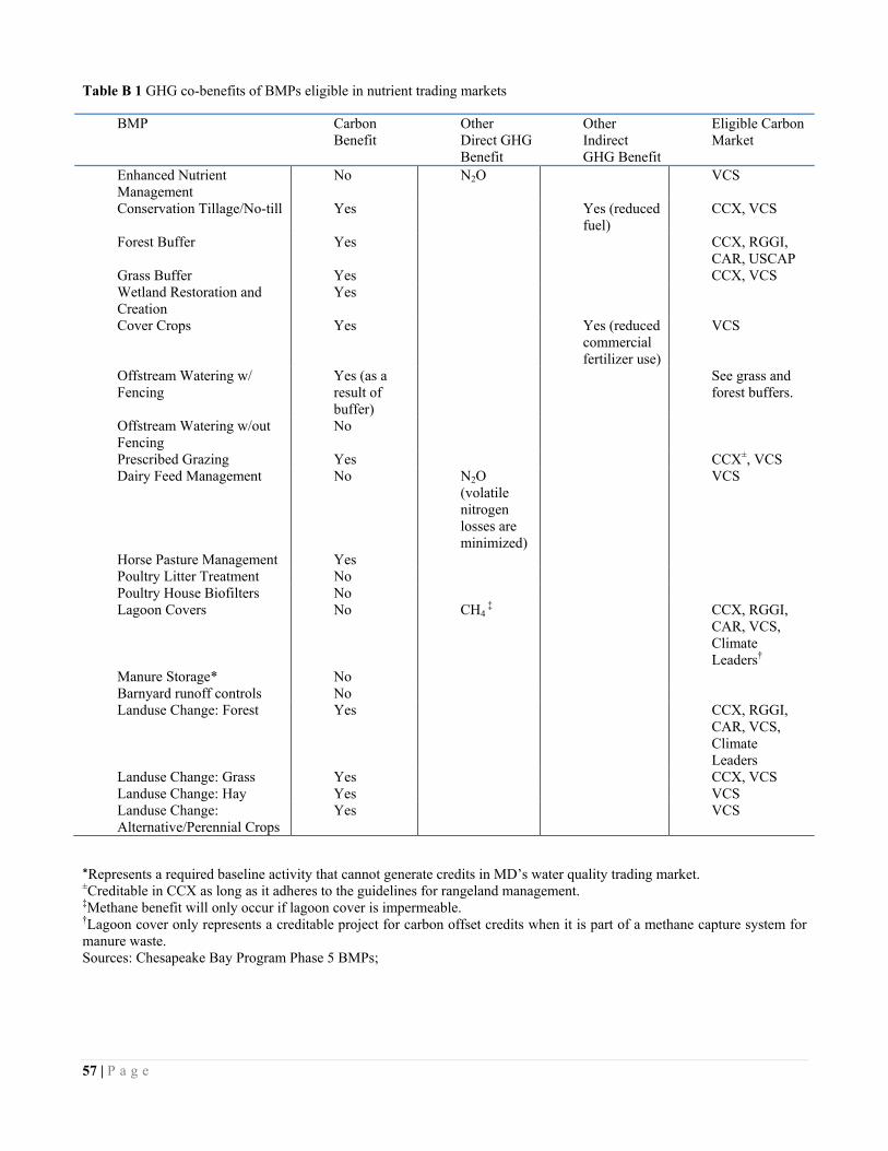
57 | P a g e

Table B 1 GHG co-benefits of BMPs eligible in nutrient trading markets

BMP Carbon Benefit

Other Direct GHG Benefit

Other Indirect GHG Benefit

Eligible Carbon Market

Enhanced Nutrient Management

No N2O VCS

Conservation Tillage/No-till Yes Yes (reduced fuel)

CCX, VCS

Forest Buffer Yes CCX, RGGI, CAR, USCAP

Grass Buffer Yes CCX, VCS Wetland Restoration and Creation

Yes

Cover Crops Yes Yes (reduced commercial fertilizer use)

VCS

Offstream Watering w/ Fencing

Yes (as a result of buffer)

See grass and forest buffers.

Offstream Watering w/out Fencing

No

Prescribed Grazing Yes CCX±, VCS Dairy Feed Management No N2O

(volatile nitrogen losses are minimized)

VCS

Horse Pasture Management Yes Poultry Litter Treatment No Poultry House Biofilters No Lagoon Covers No CH4

‡ CCX, RGGI, CAR, VCS, Climate Leaders†

Manure Storage* No Barnyard runoff controls No Landuse Change: Forest Yes CCX, RGGI,

CAR, VCS, Climate Leaders

Landuse Change: Grass Yes CCX, VCS Landuse Change: Hay Yes VCS Landuse Change: Alternative/Perennial Crops

Yes VCS

*Represents a required baseline activity that cannot generate credits in MD’s water quality trading market. ±Creditable in CCX as long as it adheres to the guidelines for rangeland management. ‡Methane benefit will only occur if lagoon cover is impermeable. †Lagoon cover only represents a creditable project for carbon offset credits when it is part of a methane capture system for manure waste. Sources: Chesapeake Bay Program Phase 5 BMPs;

   

58 | P a g e

B2. Water Quality Trading Markets in the Chesapeake Bay

Introduction & Background The Chesapeake Bay is the largest estuary in the United States. It is an incredibly complex ecosystem that includes important habitats and food webs, in addition to sustaining sizeable fisheries and recreation interests. The Chesapeake Bay watershed stretches across more than 64,000 square miles, encompassing parts of six states—Delaware, Maryland, New York, Pennsylvania, Virginia and West Virginia—and the entire District of Columbia. However, most of the Chesapeake Bay and many of its tidal tributaries are impaired and no longer able to sustain the many species which once thrived in its waters. Sediment and nutrient over-enrichment as well are responsible for the degradation of the Bay’s water quality. Nutrients (primarily nitrogen and phosphorus) and sediments enter the Bay from point sources (e.g., wastewater treatment plants), and from nonpoint source runoff (e.g., agricultural runoff). Nutrient over-enrichment, or eutrophication, stimulates the growth of algal blooms that block sunlight from penetrating the water’s surface and consume dissolved oxygen, creating uninhabitable hypoxic or anoxic conditions for the Bay’s living resources. In 2002, the Chesapeake Bay states, Maryland, Virginia, Pennsylvania, District of Columbia, and West Virginia, signed the Chesapeake Bay Water Quality Initiative (CBWQI) which committed the signatories to cooperate on efforts to protect and restore the Bay and its tributaries. As part of the 2002 CBWQI, each jurisdiction within the Chesapeake Bay watershed agreed to develop its own Tributary Strategy that will serve as an implementation plan outlining steps and goals for achieving agreed upon pollution allocations for nutrient and sediment loads by 2010. Because states were unable to show adequate progress towards meeting their nutrient reduction goals in 2010, the entire Chesapeake Bay watershed will be subjected to a Total Maximum Daily Load (TMDL). A TMDL is a “pollution diet” that identifies sources of pollution and allocates nutrient reduction targets to emitting sectors. In essence the TMDL allocation process is not much different from that of the voluntary Tributary Strategy process, the difference being that the TMDL is a regulatory framework under the Clean Water Act (CWA). As a result of nutrient reduction obligations under the Tributary Strategies and imminent requirements under the TMDL (which is still in development), the Maryland, Pennsylvania, Virginia and West Virginia have or are planning to implement caps for total nitrogen (TN) and total phosphorus (TP) through issuance of National Pollution Discharge Elimination System (NPDES) point sources regulated under the Clean Water Act (CWA)—mainly wastewater treatment plants (WWTPs).17 The nutrient caps on point sources are also motivated by Maryland’s adoption of water quality standards for the Bay in 2004. The CWA requires states to ensure that they do not prevent the attainment and maintenance of downstream water quality standards; thus all states upstream of the Bay must ensure that water quality standards are met. In conjunction with their intent to implement nutrient caps for WWTPs, Virginia, Pennsylvania, Maryland, and West Virginia have developed (or are developing) water quality trading programs. Water quality trading programs can serve two distinct purposes: first as a cost-control measure that allows regulated sources to achieve caps through least-cost solutions, and secondly as a watershed cap-

17 Sediment reductions called for in the tributary strategies are not included in water quality trading programs as currently designed. Wastewater treatment plants do not discharge sediment in large quantities and are thus not regulated for sediment.

59 | P a g e

maintenance mechanism that allows for growth in the watershed while keeping nutrient levels steady through offsets trading. In the first instance, water quality trading is a market-based approach that can help jurisdictions meet water quality targets more cost-effectively than with regulations and voluntary programs alone. Water quality trading allows regulated sources the most flexibility in meeting their permitted limit (or individual cap) and is premised on the fact that the costs to reduce pollution differ among individual entities depending upon their size, location, scale, management, and overall efficiency. Trading allows sources with high abatement costs (e.g. wastewater treatment plants and stormwater utilities) to purchase pollution discharge reductions from sources that have lower abatement costs (e.g. agricultural operations). Such transactions can result in the efficient allocation of pollution reduction responsibilities to economically lower pollution discharges below required levels. Water quality trading is also an important tool that allows for growth under a watershed-wide nutrient cap. Within a watershed that is capped under a TMDL, new or expanding sources within the watershed that have no current allocation can purchase offsets from other sources within the watershed that reduce their nutrient discharges below required levels. Water quality trading can take many forms, with the most straightforward being trades between two regulated point sources such as wastewater treatment plants—one that has reduced nutrient discharges below its permitted level and another that is currently discharging above its permitted level. However, water quality trading can also take place between regulated point sources and unregulated nonpoint sources such as agriculture. In the Chesapeake Bay, state water quality trading programs include both point-to-point and point-to-nonpoint trading. The purpose of this section is to provide an overview of the various state water quality trading programs, with a special emphasis on the treatment of agricultural nonpoint sources within these programs. There are often multiple benefits to the types of practices that agricultural operations use to reduce nutrients, allowing for the possibility of generating credits for ecosystem services beyond water quality (e.g., greenhouse gas reductions, habitat creation, soil conservation). By providing background on the role of agricultural nonpoint sources in water quality markets in the Chesapeake Bay, we hope to identify ways in which farmers and state agencies might capitalize on the synergies surrounding various environmental markets. State Water Quality Trading Programs As a means for allowing regulated (or capped) sources the most flexibility in meeting their permitted limit (or individual cap), as well as a means for allowing for growth in a watershed that has capped nutrient discharges from WWTPs, Pennsylvania, Virginia, West Virginia, and Maryland have begun to develop and implement water quality trading programs. Unlike the carbon markets, there is no formal terminology to distinguish trading among regulated sources and trading between regulated and unregulated sources. However, to create a consistency in terminology, this paper refers to trades between capped and uncapped sources (e.g. regulated wastewater treatment facilities and agricultural sources) as offsets trading, while trading between two capped sources will be referred to as allowance trading (analogous to emissions trading in the carbon markets).

60 | P a g e

In general, the state water quality trading programs will become active in 2010 or later once nutrient discharge requirements for regulated sources become active within permits. Table 2 provides a summary of the permit requirements for regulated sources, and the allocation policy for nutrient discharges of new and expanding sources. Virginia Virginia was the first state within the Chesapeake Bay watershed to issue nutrient trading rules. Legislation was passed in 2005 to create the Chesapeake Bay Watershed Nutrient Credit Exchange Program and provides Virginia’s wastewater treatment facilities in the Bay watershed with the opportunity to meet required nutrient reductions through trading. The Virginia program stipulates that existing point sources will have the option of meeting their forthcoming permit requirements using upgrades, reclamation and reuse of wastewater, and/or trades with other point sources. New and expanding plants must obtain offsets from nonpoint sources such as agriculture. Most point sources in Virginia have elected to join the Virginia Nutrient Credit Exchange Association—a trading association that will manage the exchange credits (allowances) between point sources. The members of the Exchange plan to comply with upcoming NPDES permit limits through a combination of plant upgrades and credit sales among members. It is not expected that facilities that currently have allowances will need nonpoint source offsets to meet their cap.

At present there are 30 to 45 new and expanding WWTPs planned within Virginia’s Chesapeake Bay watershed area with a capacity of greater than 0.04 million gallons per day (mgd). These facilities will receive no allocation for the discharge of total nitrogen (TN) or total phosphorus (TP) in their permits.18 New facilities must be designed to the limit of technology for nutrient removal and must offset 100 percent of their actual TN and TP discharge. Existing facilities undergoing expansion must obtain nonpoint source offsets or upgrade technology. If they are unable to locate sufficient reductions from nonpoint source offset projects, they can pay into the state-sanctioned Water Quality Improvement Fund. In turn, the Water Quality Improvement Fund will then identify and fund nonpoint source offset projects to generate the needed reductions. Pennsylvania Pennsylvania was the next state to develop a water quality trading policy, issuing guidance in 2006. Pennsylvania permit limits for TN and TP are applicable to all facilities with capacities greater than 0.2 mgd, which is a total of 251 plants.19 Permits will be issued in five phases beginning in 2010. Facilities may upgrade to meet permit limits, obtain allowances from other capped sources, or purchase offsets from uncapped sources (e.g. agriculture). Pennsylvania has stipulated that new and expanding facilities planned after 2007 (regardless of size) will be given no discharge allowances for TN and TP—thus, these facilities will need to offset all TN and TP they expect to discharge through the purchase of allowances from other point sources, or through purchase of offset credits. Unlike Virginia, existing WWTPs have not created a trading

18 Personal communication with Allan Brockenbrough of Virginia Department of Environmental Quality. 19 State negotiations and different Chesapeake 2000 commitments resulted in varying output standards for TN and TP permit limits in each state.

Table B 2 State Water Quality Trading Programs

State Permit/Technology limits (individual caps)

Permit issuance Growth allocations

Maryland Existing majors (greater than .5 mgd) must upgrade to ENR and operate at concentrations of 4 mg/L N and .3 mg/L P. Existing minors (less than .5 mgd) have no technology requirements.

Technology requirement to upgrade to ENR is in effect.

No allocations for new or expanding facilities of any size.

Pennsylvania Existing major facilities will be capped at 6 mg/L N at design flow and .8 mg/L P at design flow. Currently, facilities with flow of less than .2 mg will only be given monitoring requirements, with possibility of caps in the future.

NPDES permits reflecting nutrient limits will become effective in three phases. Phase 1 facilities represent major dischargers and will be issued permits in October of 2001. The remainder of permits will be issued in 2012 and 2013.

No allocations for new or expanding facilities of any size.

West Virginia (under development)

Existing major facilities will be capped at 5 mg/L N at design flow and .5 mg/L P at design flow. Minor facilities will have no requirements beyond monitoring.

Permits being issued on rolling basis. No allocation for new or expanding facilities greater than .05 mgd

Virginia Existing major facilities will receive caps for nutrients based on their trading basin. Eastern Shore: 4 mg/L N, .3 mg/L P Potomac AFL: 4 mg/L N, .3 mg/L P Potomac BFL: 3 mg/L N, .3 mg/L P James: 6 mg/L N, .5 mg/L P Rappahannock: 4 mg/L N, .3 mg/L P York: 6 mg/L N, .7 mg/L P

Compliance dates under the General Watershed Permit will vary by river basin, based on ability to achieve compliance.

No allocation for new or expanding facilities greater than .04 mgd

61 | P a g e

association and are not limited to meeting their individual cap only through allowance trading. To date, two wastewater treatment facilities (Mt. Joy Borough and Fairview Township) have already brokered trades for the purchase offsets from agricultural sources. These trades will come into effect in 2010 when permits are issued. In addition, the Harrisburg wastewater treatment plant has recently issued an RFP for 1.9 million offsets annually for five to ten years West Virginia West Virginia has recently submitted its final trading guidance for public comment. West Virginia plans to issue permit limits for TN and TP for existing major WWTPs on a rolling basis (as permits are renewed). WWTPs that do not meet permit requirements will have the option of upgrading their facility to meet effluent requirements, performing upgrades on minor WWTPs not subject to the TN and TP limits, obtaining credits through septic hookups, purchasing allowances from other regulated sources, or purchasing offsets from unregulated sources (e.g., agriculture). In addition, no new allocation for TN and TP discharges will be given to new and expanding facilities greater than 0.05 mgd. New and expanding sources must offset 100 percent of their new nitrogen and phosphorus loads through purchase of allowances or reductions from offsets projects. Maryland Maryland is unique in that it currently has a technology requirement for all major wastewater facilities. The 2004 Chesapeake Bay Restoration Act mandated that all major wastewater treatment facilities were to upgrade to Enhanced Nutrient Removal (ENR) technology while at the same time, implementing a statewide sewer fee on households to finance the upgrades. The technology requirements cover the 65 major dischargers in Maryland. Facilities cannot trade to meet the technology requirement. However, recognizing that it needed a strategy for controlling nutrients from wastewater treatment plants in the face of regional growth, Maryland has developed an offsets program for new and expanding wastewater treatment facilities. Phase 1 of the offset policy has been finalized. It describes how new or expanding wastewater treatment facilities can acquire offsets by upgrading minor dischargers to ENR. Phase 1 also provides guidelines on how wastewater treatment plants can generate offsets by connecting residential onsite sewage disposal systems to their ENR facilities. Point sources will receive offset credits for 12.2 pounds of nitrogen per year for every septic hookup in a critical area, 7.5 pounds of nitrogen for every septic hookup within 1,000 feet of perennial surface waters, and 4.6 pounds of nitrogen elsewhere. Septic hookups do not generate phosphorus offset credits. The Phase 2 offset policy has been issued as draft documents and outlines how new and expanding facilities can purchase nutrient offsets from nonpoint sources (primarily agriculture). The state is also planning a Phase 3 policy that will describe an offset policy for stormwater and other urban nonpoint trading. Trading Basins Each state has established trading areas or basins that define where trades can occur. The trading basins are based on watersheds with the exception of Maryland. Maryland combined the Susquehanna, Eastern Shore and Western Shore into a single trading basin labeled “Everywhere

62 | P a g e

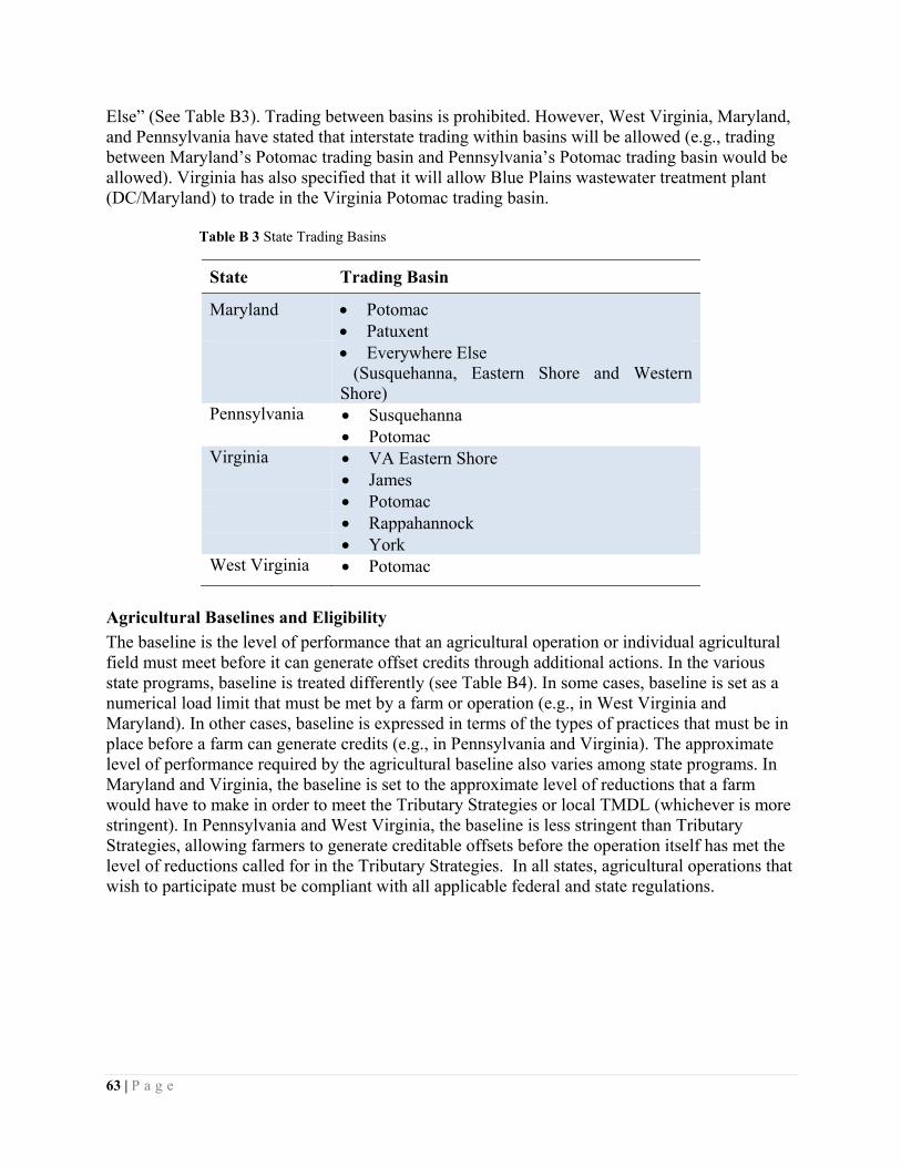
Else” (See Table B3). Trading between basins is prohibited. However, West Virginia, Maryland, and Pennsylvania have stated that interstate trading within basins will be allowed (e.g., trading between Maryland’s Potomac trading basin and Pennsylvania’s Potomac trading basin would be allowed). Virginia has also specified that it will allow Blue Plains wastewater treatment plant (DC/Maryland) to trade in the Virginia Potomac trading basin.

Table B 3 State Trading Basins

State Trading Basin

Maryland • Potomac • Patuxent • Everywhere Else

(Susquehanna, Eastern Shore and Western Shore)

Pennsylvania • Susquehanna • Potomac Virginia • VA Eastern Shore • James • Potomac • Rappahannock • York West Virginia • Potomac

Agricultural Baselines and Eligibility The baseline is the level of performance that an agricultural operation or individual agricultural field must meet before it can generate offset credits through additional actions. In the various state programs, baseline is treated differently (see Table B4). In some cases, baseline is set as a numerical load limit that must be met by a farm or operation (e.g., in West Virginia and Maryland). In other cases, baseline is expressed in terms of the types of practices that must be in place before a farm can generate credits (e.g., in Pennsylvania and Virginia). The approximate level of performance required by the agricultural baseline also varies among state programs. In Maryland and Virginia, the baseline is set to the approximate level of reductions that a farm would have to make in order to meet the Tributary Strategies or local TMDL (whichever is more stringent). In Pennsylvania and West Virginia, the baseline is less stringent than Tributary Strategies, allowing farmers to generate creditable offsets before the operation itself has met the level of reductions called for in the Tributary Strategies. In all states, agricultural operations that wish to participate must be compliant with all applicable federal and state regulations.

63 | P a g e

Table B 4 Current State Baseline Requirements for Agriculture

State Agricultural Baseline Requirements Pennsylvania To meet baseline, farmers must be in compliance with applicable federal and

state laws, have an implemented nutrient management plan, and have implemented one of the following best management practices:

• 100 Foot setback or equivalent; this is achieved when ONE of the following is met:

o Manure is not mechanically applied within 100 feet of surface water; o There are no surface waters on or within 100 feet of the farm; o Farm uses no manure application and applies commercial fertilizer at

or below the Penn State recommended agronomic rates. OR

• 35 Foot buffer or equivalent; this is achieved when all of the following are met:

o A minimum of 35 feet of permanent vegetation is established and maintained between the field and surface water.

o Area can be grazed or cropped under a specific management plan, and permanent vegetation must be maintained at all times. (Permanent vegetative buffers 50’ or greater in width may qualify to generate nutrient reduction credits.)

OR • 20 % reduction option

o A reduction of 20% in the farm’s overall nutrient balance beyond baseline compliance.

Virginia To meet baseline, farmers must implement the following best management

practices that are applicable to their operation: • soil conservation (i.e., the operation must achieve soil loss tolerance value of

T or less), • implemented nutrient management plan, • cover crops (late planting), • streambank fencing with a minimum 35 foot set-back (pasture only), and • 35 foot vegetated riparian buffers

Maryland To meet baseline, farmers must achieve modeled Tributary Strategy nitrogen and

phosphorus load targets for all fields within the candidate parcel or tract (alternately, the parcel or tract might be subject to the TMDL nitrogen and phosphorus load targets if applicable). These loads will vary by watershed segment/TMDL watershed. Maryland also requires that the agricultural operation be in compliance with all applicable federal and state laws, and have an implemented nutrient management plan. Baseline for confined animal operations is defined by having an implemented comprehensive nutrient management plan, adequate manure storage, and mortality composting.

West Virginia (under development)

To meet baseline, farmers must achieve modeled 2005 nitrogen and phosphorus load levels for agricultural land on the field where credits will be generated. In addition, the entire farm must comply with applicable federal and state laws and have an implemented nutrient management plan.

64 | P a g e

65 | P a g e

It is important to note that as a result of the Bay-wide TMDL, which is expected to be final in 2011, agricultural baselines within the state trading programs might have to change. EPA guidelines state that trading programs within TMDL watersheds must ensure that nonpoint sources meet their allocation under the TMDL before they can trade. This likely means that all states will have to set their baseline requirements for agriculture equal to the allocations set forth by the TMDL. Credit Generating Activities Agriculture-related activities that can generate offset credits in the Chesapeake Bay water quality trading markets are generally those practices that are beyond baseline and that have been vetted by the Chesapeake Bay Program office and have approved nutrient reduction efficiencies. Table 5 is a list of best management practices and nutrient reduction efficiencies that have been approved by the Chesapeake Bay Program and can be installed to generate offsets on agricultural land. In addition to approved best management practices, states have agreed to review new and emerging nutrient reduction methodologies that are not on the approved list.  

Additionality Provisions for Agricultural Offsets Additionality provisions refer to the policy decisions that are made to ensure that nutrient offsets from agricultural sources are additional to the nutrient reductions that agriculture has already made or should be making. Additionality provisions for agricultural sources vary among the state water quality trading programs. Each state program stipulates that actions eligible to generate creditable reductions must be additional. That is to say, a farmer cannot generate creditable reductions today from a practice that he implemented five years ago. The exceptions to this rule are annual agronomic practices such as conservation tillage, cover crops, etc., that farmers reconsider and reimplement every year. In order to avoid a disincentive to farmers who are already implementing annual agronomic practices, the states decided to accept annual agronomic practices as “additional” practices each year that they are implemented. Additionality guidelines also include provisions for eligibility of practices implemented with federal and/or state cost share funding. Maryland and Virginia forbid practices that are funded with cost share funds from generating creditable offsets. The logic being that a cost-shared practices do not meet the definition of additional as they would have happened anyway, and that were farmers allowed to sell these practices it would constitute “double-dipping.”20 Instead, Virginia and Maryland state that cost share funding should be used to fund “below-the-baseline” practices that help farmers meet Tributary Strategies. Pennsylvania and West Virginia, however, do allow practices implemented with cost share to generate offsets. Lastly, the baseline requirements for agriculture (described in previous section) help determine additionality. Baselines determine a level of performance that a landowner must achieve before he can generate creditable offsets. Baselines help ensure that reductions that should have happened anyway (based on expected levels of performance) are not creditable in the marketplace. Furthermore, Virginia and Maryland have set baselines at a level that is equivalent

20 Note that Maryland does allow for previously cost-shared practices to generate credits once the cost-share contract expires. For example, a buffer installed with CREP money might contractually obligate the farmer to keep and maintain that buffer for 10 years. Once that 10 year contract expires, the farmer might then be able to generate credits for that same practice as long as the buffer were still in place.

to the Tributary Strategies, thus ensuring that the offsets generated by agriculture are additional to those reductions called for in the Tributary Strategies. Table B 5 Best management practices and associated nutrient efficiencies

BMP TN TP

Conservation Planning* 3-8% 5-15% Nutrient Management Plan Application

reduction Application reduction

Enhanced Nutrient Management 7% 0% Decision Agriculture 4% 0% Conservation tillage Landuse change Landuse change Continuous No-till 10-15% 20-40% Forest Buffer

19-65% + Landuse change (applied to upland acres)

30-45% + Landuse change (applied to upland acres)

Grass Buffer

13-46% (applied to upland acres)

30-45%

Wetland Restoration and Creation

7-25% + Landuse change (applied to drainage area)

12-50% + Landuse change (applied to drainage area)

Cover Crops (varies by region, cover crop type, planting date, and seeding method)

9-45% 0-15%

Commodity Cover Crop (varies by region, cover crop type, planting date, and seeding method)

5-17% N/A

Stream Access Control w/ Fencing Credited as riparian buffer

Credited as riparian buffer

Alternative Watering Facility 5% 8% Perscribed Grazing/PIRG 9% 24% Forest Harvesting 50% 60% Dairy Feed Management Application

reduction Application reduction

Horse Pasture Management N/A 20% Mortality Composting 40% 10% Poultry Litter Treatment 50% (ammonia

only) N/A

Poultry House Biofilters 60% (ammonia only)

N/A

Lagoon Covers 15% (ammonia only)

N/A

Manure Storage* 75% 75% Barnyard Runoff Control/Loafing Lot Management

20% 20%

Water Control Structure 33% N/A Land Retirement Landuse change Landuse change Landuse Change: Hay Landuse change Landuse change Landuse Change: Alternative/Perennial Crops Landuse change Landuse change Tree Planting Landuse change Landuse change

Source: Chesapeake Bay Program Office. Phase 5 CBWM efficiencies. Updated April 28, 2010.

66 | P a g e

Credit LifeCredit life is defined in the same way in each of the state water quality trading programs. Agricultural credits are generated on an annual basis. Offsets must be generated and used in the same year. Unlike the carbon markets, water quality trading programs do not allow for banking of credits for use in future years as water quality standards must be met each year. If water quality goals require that 100 pounds of nitrogen must be reduced annually to meet water quality standards, then reducing 150 pounds in year one and only 50 pounds in year two would result in violation of water quality standards in the second year. Because of the annual nature of credits in water quality markets, permanence is not a requirement of offset projects. For example, a farmer might install a riparian buffer to generate credits. Any future decision to remove the buffer would not affect the validity or effectiveness of nutrient reductions the buffer generated during the period in which it was implemented and maintained. Certification and Verification In general, states certify offset projects once an application has been received, reviewed, and approved by the proper entities. In Maryland, Pennsylvania, and West Virginia, certification of an offset project can happen before practices have been put in the ground. Certification implies that if the offset project, as outlined in the application, were to be put in place, they would generate x number of creditable offsets. These offsets are then registered and available for exchange. Verification refers to assurances that offsets projects that have been certified are actually in the ground. The exchange of credits will trigger the verification stage. Credits cannot be formally exchanged or applied towards permit requirements until they have been verified. Verification procedures will generally rely on on-site inspections that ensure that the activity is in the ground and implemented according to specifications. Verifications are required annually via approved third-party verifiers. The states have pledged to perform annual audits on a portion of certified projects as well. If the verification process reveals that a project is not being implemented as planned, the project and associated credits will be nullified. Role of Aggregators Aggregators are entities that purchase credits (generally large quantities of nonpoint source offsets) to re-sell them to interested buyers. In water quality trading markets, aggregators serve two purposes. First, they bundle small quantities of credits from diverse sellers and re-sell them in the larger quantities demanded by point sources. Thus, in lieu of finding and contracting sales of offsets with multiple small sellers, the point source can perform a single transaction with an aggregator. Secondly, aggregators represent a mitigated liability risk for the buyer. By introducing an aggregator, the direct liability link between the regulated entity and the unregulated nonpoint source entity is severed. Because an aggregator deals with large portfolios of projects, it can more easily mitigate risks associated with delivery and performance of those projects. For example, an aggregator might sell only a portion of credits from its offsets portfolio and keep the remainder in reserve should one or more of the offsets projects fail or not get implemented as promised. Aggregators are optional in water quality markets, and farmers are able to sell credits from offsets projects directly to regulated sources if they wish to.

67 | P a g e

68 | P a g e

B3.Voluntary and Regulatory Carbon Markets

Background and Introduction The worldwide carbon markets can be divided into two segments: the voluntary markets and the regulatory (compliance) markets. Voluntary carbon markets include all carbon offset trades that are not required by regulation. The voluntary carbon markets themselves have two distinct components: the Chicago Climate Exchange (CCX), which is a voluntary but legally binding cap-and-trade system, and the broader, non-binding “Over-the-Counter” (OTC) offset market. The total value of transactions in the voluntary carbon markets is estimated at $705 million for 2008. 21The average price of a voluntary carbon credit in 2008 was $7.34/tCO2emissions (increase of 22 percent from $6.10/tCO2e in 2007, and 79 percent from $4.10/tCO2e in 2006).22 Table B6 shows current offset prices in various markets. Table B 6Carbon Offset Prices (2008)

Carbon Credit Program Offset Prices CCX (Chicago Climate Exchange) $4.43/tCO2e VCS (Voluntary Carbon Standard) $5.50/tCO2e CAR (Climate Action Reserve) $8.90/tCO2e

The development of regulated carbon markets in the United States has been fragmented due to a lack of federal regulation. To date there have been a handful of regional attempts at regulating greenhouse gas emissions, most notably the Regional Greenhouse Gas Initiative (RGGI) which includes ten northeast and mid-Atlantic states. The purpose of this section is to give an overview of some of the regulatory and voluntary carbon markets that exist in the United States. More specifically this section examines the offset provisions of various markets and explores in more detail the types of offset projects that pertain to Maryland farmers and landowners. We will examine the role that agriculture has played or will play in these markets, including opportunities for generating credits as well as baseline and eligibility requirements. National and Regional Carbon Markets Emissions vs. Offsets Trading In carbon markets, there are two types of trades, emission trading and offsets. In emissions trading both participants are capped. Participants might be countries or individual. Individual companies or countries that reduce emissions below their targets or caps can sell the excess emissions. Meanwhile countries or companies that cannot cost-effectively reduce emissions to their target levels can purchase emission allowances. By contrast, carbon offsets are reductions from uncapped sectors or sources that are used for compliance with the cap. Because reducing emissions from unregulated sources can be less costly than at capped sources, offsets can lower the costs associated with achieving the cap.

21 See “Fortifying the Foundation: State of the Voluntary Carbon Markets 2009.” Ecosystem Marketplace. 2009. Available at http://www.forest-trends.org/documents/files/doc_2343.pdf. 22 Ibid.

The following sections will examine the types of offsets projects that are eligible to be undertaken by agricultural operators or other landowners to generate GHG reductions within the various carbon markets. Regional Greenhouse Gas Initiative (RGGI) RGGI includes ten Northeast and Mid-Atlantic states (CT, DE, ME, MD, MA, NH, NJ, NY, RI, VT) in its market-based carbon dioxide emissions reduction program. These ten states have capped carbon dioxide emissions from the power-generating sector, and require a 10 percent reduction in emissions by 2018. Individual trading programs in each state are linked through RGGI, so the state programs can function as a collective market for carbon emissions and allow any regulated power plant to use CO2 allowances issued by any of the 10 participating states. Each allowance represents one ton of emitted carbon dioxide. States and power plants can comply with greenhouse gas emission caps through individual actions that include improving energy efficiency at the plant, employing technologies to reduce out-of-stack emission (i.e., carbon capture and storage technologies), or switching to low-carbon or carbon neutral fuels. Alternatively, power plants can trade or use offsets to comply with their cap. As of now, there are two approved offset project types that are related to agriculture and forestry: afforestion and agricultural manure methane capture. Establishing emissions baselines, determining emissions reductions or carbon sequestration rates, and monitoring and verification may be determined by each state’s own regulations, but criteria set for regulating offset projects in RGGI’s Model Rule has been adopted by all jurisdictions.

• Afforestation. In order to ensure additionality, an afforestation project must occur on land that has been in a non-forested state for at least 10 years preceding the commencement of the project. Approved afforestation projects must be managed in accordance with sustainable forestry practices and designed to promote native forests by using native species and avoiding invasive non-native species. Furthermore, afforestation projects require a permanent conservation easement which will ensure that the new forested area remains in a forested state for perpetuity. Offsets are awarded based on the amount of net additional carbon sequestered relative to a base-year carbon measurement or previous reporting period measurement. The baseline rate of carbon sequestration is based on live above-ground biomass, live below-ground biomass, soil carbon, and dead organic matter mass. Net carbon sequestered during the reporting period is also discounted by 10 percent prior to the award of CO2 offset allowances to account for potential project reversals of carbon sequestration, unless the project sponsor retains long-term insurance, approved by the relevant state agency where the offset project is located, that guarantees replacement of any lost sequestered carbon for which CO2 offset allowances were awarded.

• Manure Methane Capture. In the case of manure management offset projects, the

methane (CH4) from animal manure and organic food waste is captured and destroyed using anaerobic digesters. Methane digester projects that generate and sell electricity back to the grid using newly captured methane are not eligible to generate offsets in RGGI unless the project is located on a farm with 4,000 or fewer head of dairy cows, and/or the offset project is located in a state where market penetration of anaerobic

69 | P a g e

digester projects is 5 percent or less. Furthermore, 50 percent or more of organic waste used in eligible digester projects must originate from livestock manure. Emissions reductions are determined based on the potential emissions (in tons of CO2-equivalent) of the methane that would have been produced and emitted in the absence of the offset project under a baseline scenario that represents site-specific uncontrolled anaerobic storage conditions.

The initial crediting period for all offset projects is 10 years. Once a project is approved, it can be renewed for an additional 10 years, pending project resubmission and regulatory approval. For afforestation offset projects however, the initial period is 20 years and the renewal period is for additional two 20-year periods, pending re-approval. RGGI distributes the majority of its CO2 allowances during quarterly auctions, the first of which took place in September of 2008. To date, over 134 million allowances have been sold for the 2009 year, representing over 400 million dollars. However, because allowance prices have been so low ($2.19 in the most recent auction), there is not yet a market for offsets, including agricultural offset projects. As such, no offset projects have been registered through the RGGI website, and no offsets have been sold. Chicago Climate Exchange The Chicago Climate Exchange (CCX) was launched in 2003 as a voluntary greenhouse gas emission cap and trade scheme in North America. It has since expanded its geographic scope; offsets have been generated by projects in countries outside the US, including India, China, Germany, and others. Although participation is voluntary, once entities elect to participate in CCX, compliance with emission reduction targets is binding. In the first phase of the scheme, from 2003 to 2006, CCX members agreed to cut their emissions by one percent each year below their annual average emissions for the period 1998 to 2001, thereby achieving a reduction of four percent by the end of the fourth year. For the second phase from 2007 to 2010, the original members agreed to cut their emissions by an additional 0.5 percent each year to achieve an overall target of six percent below 1998–2001 levels by 2010. New members participating in the second phase must achieve a similar overall reduction target by 2010 by reducing their emissions by 1.5 percent each year. Members can comply either by cutting emissions internally, trading emission allowances with other CCX members, or purchasing offsets generated under the CCX offset program, including agricultural offset programs. Offsets may only be used to meet up to 50 percent of compliance standards, and currently account for approximately 15 percent of all emissions reductions achieved under the program. Farmers can participate in offset projects in the following ways: agricultural methane collection and combustion, soil carbon sequestration (continuous conservation tillage and grassland conversion), forestry carbon sequestration, and sustainable rangeland management.

• Agricultural Methane Collection and Combustion. Farmers can qualify for methane capture offset programs by installing an anaerobic digester as long as projects employ one of the following baseline manure management practices: liquid slurry, pit storage

70 | P a g e

beneath animal confinement, or anaerobic lagoon.

CCX uses a specific equation to measure the baseline amount of methane produced. The type of manure storage system (e.g., liquid slurry, pit storage anaerobic lagoon), type of animal, and state are all factors that affect the baseline methane value. A table is published on the CCX website with emission factors for species, type of management system, and state.

• Soil Carbon Sequestration. Continuous conservation tillage and grassland conversion

offset credits vary from state to state, based on the regional climate. An appendix on the CCX website provides sequestration rates for every county in the United States. Rates range from 0.6 metric tons per acre to 0.2 tons per acre. CCX draws a distinction between conservation tillage and continuous conservation tillage: only when the same land is continually (yearly) plowed in a non-inversion manner that maintains at least 30 percent crop residue cover is it eligible to be used as an offset project. Conversion from cropland to grassland also qualifies for offsets. Basic specifications require a minimum of a five-year contractual commitment, either to continuous conservation tillage or grassland conversion. Such carbon sequestration projects must be enrolled through an offset aggregator.

CCX has named two baseline scenarios to qualify conservation tillage an offset project: 1. Current practices that continue on the cropland either resulting in a loss of soil carbon

through conventional tillage or intermittent conservation tillage practices or no net gain in soil carbon, and

2. Continuous conservation tillage practices that are implemented without the benefit of carbon offset revenue.

• Forestry Sequestration. Offsets are issued for Forestry Sequestration projects on the basis of increases in ‘carbon stocks,’ specifically above-ground biomass, below-ground biomass, soil organic carbon, standing dead trees, down dead wood, and forest floor portions. In order to insure additionality, project owners must commit to sequester additional carbon in their forests based on a baseline inventory calculated at the beginning of a project. The project owner is credited with offsets when the forest generates positive amounts of carbon above their baseline value, and debited when forests are managed in a way that carbon storage decreases. Planting for afforestation projects must have occurred on land that has been in a non-forest state for ten years or longer. Yearly inventory monitoring and calculations on carbon sequestration is overseen by an in-house committee, the CCX Forestry Committee, which has developed emission reduction standards based on tree species present and the geographic region.

There are two categories for Forestry Carbon Sequestration programs. The first is specific to the planting of forests on lands that have not historically (last 10 years or more) contained forests. Sustainable forestry practices do not apply in this subcategory- in other words, no removal of biomass is permitted during the contracted time (fifteen years from the date of enrollment with CCX). Quantification of sequestered carbon is calculated by the Forestry Committee (FC) using accumulation tables, and published on the CCX website.

71 | P a g e

Sustainably managed forest projects have their own rules and regulations in order to qualify as an offset project. All projects must provide evidence that their forest and forestry practices are sustainable, by presenting certification from agencies that have been approved by the CCX FC. Projects are awarded offsets based on additional net carbon sequestered from the previous year by evaluating inventory annually or by using a set of growth-and-yield calculations set by the CCX FC.

• Sustainable Rangeland Management. To be eligible to undertake a sustainable rangeland

management project, a project owner must adopt and demonstrate compliance with appropriate management techniques, including the following elements for each management unit (e.g., pasture) within the ranch: 1. Forage-animal balance, ensuring forage produced meets demand of livestock and/or

wildlife. Planned utilization should not exceed 50 percent of current year’s growth measured near the end of the grazing season;

2. Prescribed grazing schedule, addressing periods of grazing, distribution within a pasture and ranch, and management units sensitive to overgrazing or erosion (i.e., rotational grazing); and

3. Contingency plan for management under drought conditions. Rangelands enrolled shall have drought management as a part of their formal grazing plan. Other stipulations include limitations on brush removal via chemical or mechanical techniques. (These techniques are allowed provided the total acreage treated is less than 10 percent of the total acreage enrolled.)

The range of soil carbon sequestration rates for rangelands used by CCX are based on a review of scientific literature, actual soil sampling at NRCS plots, Flux tower data, and runs of the Century model using COMET-VR. Rangeland sequestration rates range from 0.12 to 0 .32 metric tons of carbon dioxide per acre per year.

The CCX agriculture offsets program is active compared to other programs examined in this report. CCX has registered offset projects in 39 states and 13 countries outside of the United States. To date, CCX has issued offsets representing over 74 million metric tons of CO2e. Furthermore, 30 percent of the 162 offset providers/aggregators are reporting offset projects in the agriculture sector. More specifically, CCX reports 18 agricultural methane offset projects, 13forestry offset projects, and 18 agricultural offset projects, all from providers/aggregators, some representing multiple states. In fact, according to the Exchange’s most recent offset report, agriculture soil carbon projects represent the single most widespread offset program, with over 21 million metric tons of CO2e registered. Climate Action Reserve (CAR) The Climate Action Reserve (formerly the California Climate Action Registry, or CCAR) was launched in 2008 as a voluntary national offsets program eight years after its predecessor organization was established by the California State Legislature to encourage the reduction of GHG emissions. CAR internally establishes standards for quantifying and verifying GHG emissions reduction projects, provides oversight to independent third-party verifiers, and issues and tracks carbon credits. These in-house protocols were established during the era of CCAR

72 | P a g e

when projects could only be registered in the state of California. The registry associated with CAR is referred to as the Climate Registry. Of 20 currently registered projects (i.e., those that have completed verification) at CAR, eight are agricultural projects (five livestock manure management operations and three conservation-based forest projects). There are currently an additional 120 offset projects that have been received but are currently awaiting verification. In total, CAR has issued over 1.8 million carbon offset credits to date. Table B 7 CCX Offset registration

Offsets Registered (MT CO2e) JUNE-AUGUST 2009

TOTAL (2004-2009 YTD)

Agricultural Methane 373,900 1,406,300

Agricultural Soil Carbon 627,600 21,679,100

Avoided Emissions from Organic Waste Disposal

20,200 20,200

Coal Mine Methane 84,800 17,874,000

Energy Efficiency 1,062,600 3,316,800

Forestry 1,021,600 11,223,800

Fuel Switching 78,700 2,356,100

Landfill Methane 1,153,300 6,121,100

Ozone-Depleting Substances

48,700 787,300

Renewable Energy 611,800 7,102,000

HFC Destruction 983,500

Wastewater Treatment Methane Recovery

44,300 44,300

TOTAL 5,127,500 72,914,500

CAR has approved two types of projects related to agriculture and forestry operations. These include manure biogas emissions control for livestock operations and afforestation projects. For all offset projects, CAR outlines two general criteria that projects must meet to be additional. First, projects must demonstrate that the reductions go beyond what is required by law (regulatory surplus), and secondly, they must demonstrate that that they go above and beyond common practice (i.e., "business as usual"). Additional requirements for agriculture and forestry-related offset projects are outlined below.

• Livestock Methane. Livestock methane management projects in the United States and its territories are eligible to register with CAR if a developer installs a Biogas Control

73 | P a g e

System. Livestock projects in Mexico may also be eligible but must use a separate protocol to register reductions with CAR. The crediting period for a livestock methane capture project is 10 years. Through February 28, 2010, projects with a start date as early as January 1, 2001 may register with CAR, but after March 1, 2010, projects must be submitted to the reserve within six months of the project start date. CAR has developed a “Livestock Calculation Tool” for all project calculations and emissions reduction reports.

For a livestock methane project to qualify to generate offsets, developers of livestock projects must demonstrate that prior to the project’s implementation the depth of the anaerobic lagoons or ponds is at least one meter in depth or is deep enough to create anoxic conditions. Projects that are implemented at new livestock facilities with no prior manure management system are eligible only if the project developer can demonstrate that uncontrolled anaerobic storage and/or treatment of manure is common practice in the industry and geographic region where the project is located.

• Forestry. CAR includes three types of forestry projects: conservation or avoided conversion projects, conservation-based forest management and regeneration of native trees, and reforestation projects. Forestry projects have a 100-year crediting period and must be verified no less frequently than every six years, and must submit annual monitoring reports.

An Avoided Conversion Project must take place on private land and must result in the permanent prevention of conversion of forestland to a non-forest land use by dedicating the land to continuous forest cover through a conservation easement or transfer to public ownership. In addition, the forest owner must provide documentation demonstrating that the type of anticipated land use conversion is legally permissible, e.g., conversion to timberlands, zoning for commercial/residential development.

An Improved Forest Management Project involves management activities that maintain or increase carbon stocks on forested land relative to baseline levels of carbon stocks as defined in Section 6.2 of this protocol. An Improved Forest Management Project is only eligible if the project takes place on land that has greater than 10 percent tree canopy cover, employs natural forest management practices (as defined by CAR’s own BMP list), does not employ broadcast fertilization, and does not take place on land that was part of a previously registered Forest Project. Eligible management activities include thinning diseased and suppressed trees to increase forest productivity, managing competitive brush species, and increasing the stocking of trees in under-stocked areas.

A Reforestation Project involves restoring tree cover on land and has minimal short-term (30-years) commercial opportunities. A Reforestation Project is eligible if the project involves tree planting or removal of impediments to natural reforestation on land that has had less than 10 percent tree canopy cover for a minimum of 10 years or has been subject to a significant disturbance that has removed at least 20 percent of the land’s above-ground live biomass. No rotational harvesting of reforested trees or pre-existing carbon in live trees during the first 30 years after project start date is permitted (unless it is needed to prevent disease). A Reforestation Project that occurs on land that has had less than 10

74 | P a g e

percent tree canopy cover for at least 10 years automatically satisfies the performance additionality criterion.

One of CAR’s registered forest management projects has received national attention. In early 2008, Pacific Gas and Electric announced it would purchase 200,000 short tons of GHG emission reductions from the Conservation Fund’s Garcia River Forest Project, a management project verified by CAR in 2007. The price of $9.71 per ton of carbon dioxide for the purchase was approved by the California Public Utilities Commission.

Climate Leaders Program Climate Leaders is an EPA-led voluntary GHG emission reduction program. Launched as an industry-government partnership in 2002, it provides guidance to companies that develop climate change strategies and recognizes their efforts. To achieve reduction goals, companies may purchase GHG reductions certified through existing regulated or voluntary markets, provided that the project adheres to approved EPA methodologies. There are two agriculture/forestry based-offset projects: reforestation/afforestation and manure management (anaerobic digesters.)

• Manure Management. To qualify as an offset, manure management/anaerobic digester projects must be additional to any regulatory requirements in addition to meeting a performance threshold that is “significantly better than average.” Specifically, if the dairy or swine operation is not currently collecting and combusting manure gas, the project is considered additional. The EPA has its own set of equations to determine baseline emissions, but methane production from the digester project can also be calculated with AgSTAR FarmWare 3.0, a program developed by EPA to assist those considering installing an anaerobic digester. Once digesters are installed and methane is flared, the rate of gas flow (monitoring period) is measured monthly.

• Reforestation/Afforestation. The Climate Leaders program does not distinguish between

afforestation and reforestation and simply defines both as the planting of trees on private cropland or pastureland that causes the land to change from non-forest to forest use, with no difference in methodology for either practice. The project must result in permanent offsets or have guarantees to that any carbon losses are are replaced in the future. In order to demonstrate additionality and be eligible to generate offsets, projects must demonstrate regulatory additionality and must meet a performance threshold as defined by the program. The Climate Leaders program utilizes the EPA-produced RAPCOE (Reforestation Afforestation Project Carbon On-Line Estimator) tool, which automates the calculation of the estimated rate of conversion to forest. RAPCOE is used both for application of the performance threshold for determining additionality, described above, as well as for baseline-setting and estimation of the gross and net offset potential of the project.

Voluntary Carbon Standard (VCS) The Voluntary Carbon Standard is an international carbon offset standard and program for approval of voluntary offsets. The VCS recognizes the Climate Action Reserve (CAR) as a program with full compatibility and linkage with VCS, and thus, all projects under CAR are allowed under the VCS program. VCS has a slew of Agriculture, Forestry, and Other Land Uses

75 | P a g e

(AFOLU) projects, all of which have a minimum 20 year crediting period and a maximum crediting period of 100 years. There are four types of AFOLU projects: Afforestation, Reforestation and Revegetation (ARR); Agricultural Land Management (ALM); Improved Forest Management (IFM); and Reducing Emissions from Deforestation and Degradation (REDD). REDD is a mechanism primarily designed to credit avoided deforestation in developing countries and is not applicable in a U.S. context. The remaining three project categories are described in more detail below.

• Afforestation, Reforestation and Revegetation (ARR). Eligible activities in the ARR project category consist of establishing, increasing or restoring vegetative cover through the planting, sowing or human-assisted natural regeneration of woody vegetation to increase carbon (C) stocks in woody biomass and, in certain cases, soils.

• Agricultural Land Management (ALM). ALM projects can be placed into three

categories: improved cropland management activities, improved grassland management activities, and cropland and grassland landuse conversions.

A. Improved cropland management activities. Improved cropland management activities include the adoption of practices that demonstrably reduce net GHG emissions from a defined land area by increasing soil C stocks, reducing soil N2O emissions, and/or reducing CH4 emissions. Practices that fall under this category include (but are not limited to): adoption of no-till; elimination of bare fallows; use of cover crops; creation of field buffers (e.g. windbreaks, riparian buffers); use of improved vegetated fallows; conversion from annual to perennial crops; introduction of agroforestry practices on cropland; improved timing of application (e.g., split application), improved fertilizer formulations (e.g., slow release fertilizers, nitrification inhibitors); improved placement of N; and reducing soil CH4 emissions in flooded rice cultivation through improved water management. B. Improved grassland management activities. These activities include the adoption of practices that increase soil C stocks and/or reduce N2O and CH4 emissions. Practices include (but are not limited to): increasing forage productivity (e.g. through improved fertility and water management); introducing species with deeper roots and/or more root growth; reducing degradation from overgrazing; reducing N2O emissions through improved N fertilizer management practices; reducing fire frequency and/or intensity to reduce N2O and CH4 emissions from burning; and reducing emissions of CH4 and N2O from grazing animals via improved livestock genetics, improved feed quality, and/or by reducing stocking rates. C. Cropland and grassland land-use conversions. Cropland conversion to perennial grass vegetation is likely to be the dominant land use conversion for ALM projects. However, some grassland conversions to cropland production (e.g., introducing orchard crops or agroforestry practices on degraded pastures) could increase soil and biomass C stocks (thereby reducing net GHG emissions). Under such conditions, these conversion practices would also be considered eligible for project certification. However, projects converting

76 | P a g e

77 | P a g e

grasslands must demonstrate that they do not harm local ecosystems as outlined in the general AFOLU guidance.

• Improved Forest Management (IFM). Activities related to improved forest management

are those implemented on forest lands managed for wood products such as sawtimber, pulpwood, and fuel wood and are included in the IPCC category “forests remaining as forests.” Only areas that have been designated, sanctioned or approved for such activities (e.g., as logging concessions or plantations) by the national or local regulatory bodies are eligible for crediting under the VCS Improved Forest Management (IFM) category. Activities to reduce emissions from unsanctioned forest degradation (e.g., illegal logging) is not eligible for crediting under the IFM category but may be creditable as a Reduced Emissions from Deforestation and Degradation activity (REDD).

Additionality In order to generate carbon offsets, a project must prove that it is additional: that is, it must ensure that the GHG offset activity would not have occurred were it not for the carbon offset market. Because offset projects allow entities under the cap to increase their emissions by an amount corresponding to the GHG reductions achieved by the offset, there must be assurances that these GHG reductions are additional and would not have taken place anyway (i.e., in the absence of a carbon offset market). Ensuring that projects are additional, however, can be difficult. There are two basic approaches to determining additionality: project-specific and standardized.

1. Project-specific approaches seek to establish baseline scenarios that ensure only the reductions that occurring beyond the baseline can be credited. The baseline is generally an emissions scenario in which there is no offsets market. A project may also face a comparative analysis of possible alternatives to determine if the proposed project is, in fact, the most likely scenario (in which case it is not additional) or if another alternative is the most likely alternative (in which the proposed project is additional).

2. Standardized approaches to determine additionality evaluate projects against consistent

criteria designed to exclude non-additional projects. Standardized criteria can include the following types of considerations:

• Project is not mandated by law; • Project is not a least-cost option (as defined by regulators); • Project is not common practice (as defined by regulators); • Project uses a specific type of technology; • Project is of a certain size; • Project is initiated after a certain date; or • Project has an emission rate lower that a pre-defined performance standard.23

23 Excerpted from Derik Broekhoff and Kathryn Zyla, “Outside the cap: opportunities and limitations of greenhouse gas offsets.” December 2008. WRI.

78 | P a g e

Permanence Once emitted to the atmosphere, GHGs reside there more or less permanently. Thus, GHG offsets must also be permanent. The permanence issue is generally a question only for carbon sequestration and storage projects since these can be reversed over time. For example, in forestry or agricultural carbon sequestration projects, carbon stored in trees or soils can be released to the atmosphere as a result of fires, harvesting, land-use changes, or other disturbances. In these cases, a mechanism is required to make reversible reductions or removals functionally equivalent to permanent reductions for the purpose of issuing offset credits. Some strategies for hedging against permanence uncertainty in sequestration and storage projects include issuing discounted credits, issuing expiring credits, and establishing an insurance or reserve system to buffer against reversals.24 Application, Verification and Monitoring In carbon markets, projects must be implemented before an offsets application is approved. For example, in the RGGI program, once a project is implemented, it must be registered and an application for consideration must be submitted within 6 months. The application must include a signed verification and monitoring report from an accredited verifier. If the application is approved by the state the offset allowances are issued to the applicant. Ongoing verification and monitoring requirements for offset project vary by project type and by the market/registry. In general verification and monitoring requirements will include on-site inspections every 1, 3 or 5 years and, in some cases, longer intervals. Role of Aggregators Small offset projects may benefit from enrolling with an offset aggregator. Aggregators are entities that serve as the administrative representative of multiple offset projects, in particular projects generating less than 10,000 tons CO2e in emission reductions per year. There are challenges for individuals working to generate their own offset projects, including marketing costs, development information, and contractual costs, and aggregators can serve as a middleman between the offset provider and the purchasing entity, e.g., CCX. By gathering multiple small projects together, aggregators can create a larger pool of credits to sell. The aggregator acts as the broker between the offset project owner and the purchasing entity by managing registration, compliance, and sales and are acting as the conduit for monitoring and verification. Aggregators do not conduct monitoring themselves; it is the job of the specific market (CCX, CAR, etc) to complete monitoring and verification. They can however assemble and manage yearly reports from producers to be sent to verifiers.

Aggregators are used most frequently with CCX. As of March 2008, there were 59 registered aggregators, a majority of which focused on methane capture and soil carbon sequestration projects. In fact, soil carbon sequestration projects are required to register with an aggregator in CCX. CAR also has registered projects with aggregators.

24 ibid

Appendix C. Model Description

The model used to perform the carbon supply analysis was created for the Nutrient Trading study using STELLA dynamic modeling software. STELLA is a software package that allows users to simulate complex systems over time by specifying a series of stocks and flows and describing the mathematic relationships that govern system behavior. Once the user has parameterized the system of interest, various scenarios and conditions can then be evaluated and compared over a user-specified time period. The software provides graphical output and allows the user to run sensitivity analyses on variables of interest. Because it can easily compare output under different scenarios, STELLA was an appropriate platform to evaluate carbon supply under the variety of different market rules of interest to MDE.

C1. Model overview

Our model simulates nitrogen loading from agriculture in the five primary watershed basins in Maryland. In each time period, nitrogen loading values are calculated based on the acreage within each land use category in the basin. Loading levels are then compared with the basin-wide Total Maximum Daily Load (TMDL) cap to determine whether basins are in compliance with the cap. Basins with loading levels greater than the TMDL will implement least-cost Best Management Practices (BMPs) from a suite of eight options. Once basins have reduced loading levels below the TMDL, they will implement BMPs only if anticipated revenue from carbon and nutrient credit sale will at least cover the cost of the project. Anticipated revenue is determined by current market prices and market participation rules, which are set by the user. The model tracks carbon supplied to the market and carbon sequestered as a result of BMP implementation over time through 2030. Model sectors and data The model is structurally composed of four interacting sectors. First, the agricultural sector simulates agricultural runoff in each the five watershed basins: Susquehanna, Eastern Shore, Western Shore, Patuxent and Potomac. Second, the BMP sector simulates seven potential activities undertaken to reduce loading: nutrient management, manure management, conservation tillage, cover crops, forest buffers, grass buffers and wetland restoration. Third, the carbon sector calculates carbon sequestered as a result of implemented BMPs. Fourth, the market sector specifies market rules and determines which market (nutrient or carbon) sources will enter and calculates the amount of carbon supplied. The data used to specify the model was primarily obtained from public sources including the US Department of Agriculture and the Maryland Department of Agriculture (MDA). The most recent BMP nitrogen reduction potential and efficiencies were also obtained from MDA. Land use and BMP application data were obtained from the Chesapeake Bay Program (CBP). Carbon sequestration potentials were obtained from a variety of sources—including EPA Technical Bulletins, USDA and peer-reviewed scientific literature—in an attempt to use the most accurate available estimates. These data sources are compiled in Table C.1.

79 | P a g e

Table C. 1 Data sources for model parameters

Parameter Data source(s) Land use (acres) Chesapeake Bay Program Fertilizer efficiencies Chesapeake Bay Program Edge-of-stream factor World Resources Institute Pre-BMP nitrogen loading levels Chesapeake Bay Program BMP application (acres) Chesapeake Bay Program BMP nitrogen reduction/efficiency Maryland Department of Agriculture BMP carbon sequestration rate EPA Technical Bulletin 1909 BMP cost Wieland et al. 2009

Modeling land use The model incorporates five primary watershed basins in the state of Maryland used in the Chesapeake Bay Model: Susquehanna, Eastern Shore, Western Shore, Patuxent and Potomac. The model calculates a pre-BMP value of delivered nitrogen (lbs N) based on the acreage in each of three land uses (high till, low till and manure) and the basin-specific nitrogen edge-of-stream loading factor (Table C.2). Pre-BMP acreage in each land use category is assumed to remain constant after 2010. However, acreage is adjusted according to BMP implementation; for example, acres converted to forest buffers or wetlands are subtracted from total agricultural land use.

Table C. 2 Nitrogen edge of stream (EOS) factors for modeled basins in MD. (Data source: CBP)

Basin N EOS Susquehanna 0.38 Eastern Shore 0.44 Western Shore 0.56 Patuxent 0.63 Potomac 0.51

Incorporating BMPs In each time period, the model first decides to implement BMPs based on a comparison between the basin-wide N loading level and the basin’s TMDL. When a basin is above its TMDL, BMPs will automatically be implemented according to the least-cost options available. The only exception to this rule is the nutrient management plan, which is implemented automatically in each time step since nutrient management plans are now required for agricultural sources in MD. When a basin is below its TMDL, BMPs will be implemented if they are cost effective given user-specified market conditions, which are discussed in subsequent sections of this Appendix. For most BMPs, implementation rate is assumed to remain at its average implementation rate between 2000 and 2008, as calculated from BMP acreage data provided by CBP (Table C.3). For cases in which BMPs were initially implemented later than 2000 (wetlands and manure management), the implementation rate is an average of all years in which data are available. In the case of grass buffers, there was a large spike in acreage between 2002 and 2003 that makes the average implementation rate artificially high. Therefore, the grass buffer implementation rate was calculated as the average implementation rate between 2003 and 2008. Nutrient

80 | P a g e

management plans are phased into compliance from 80 percent in 2008 to 100 percent by 2015 at a decreasing rate. Table C. 3 Historical BMP implementation and average implementation rates for modeled BMPs: Conservation tillage (cons tillage), cover crops, forest buffers (FB), grass buffers (GB), wetland restoration (wetland) and manure management (manure). Values in grey are not included in the average rate calculation. Acreage data were provided by CBP.

Year Cons tillage (acre)

Cover crops (acre)

FB (acre)

Wetland (acre)

GB (acre)

Manure (acre)

2000 726,538 159,773 5,469 0 2,557 02001 665,039 70,920 8,628 3,358 2,585 02002 787,725 97,755 13,376 4,471 2,593 02003 756,754 113,609 16,484 6,252 10,879 02004 747,655 52,328 17,836 6,448 12,251 31,3792005 739,244 52,302 19,050 6,707 13,506 11,0192006 733,615 124,552 19,388 6,972 15,441 13,2032007 724,548 230,474 19,704 7,108 16,049 23,6892008 719,576 179,365 19,884 7,272 16,833 20,759

Avg. rate 0.0014 0.1819 0.0387 0.0308 0.0921 0.0859 In the literature, BMP costs are typically averaged but in some cases project-to-project cost is highly variable. To incorporate this variation, we imposed a normal distribution around BMP costs so that each time a BMP is considered, its cost occurs as a function of its probability within its distribution (Figure C1). Thus, the model achieves a greater level of realism in BMP decision-making compared to use of an average cost.

Figure C. 1 Sample model run to show BMP cost variation. The BMP modeled here is a forest buffer with an imposed normal cost distribution (mean=$800/acre; SD=$25/acre).

To determine whether BMPs are cost-effective, the model calculates anticipated revenue at the current market price in 2010 dollars over the life of a project (15 years for wetlands and buffers). Costs are calculated as initial fixed costs plus variable maintenance costs over the lifetime of the

81 | P a g e

project. Initial model runs assume that the source covers the entire cost of the project including soil rental costs. Other scenarios assume that cost-sharing programs cover varying portions of the project. Results for these scenarios are presented in the main document text. Carbon sequestration As BMPs are implemented each time period, the model calculates total carbon sequestered by multiplying the sequestration value of each BMP by its total acreage (Table C.4). The model keeps track of both annual and cumulative carbon sequestration.

Table C. 4 BMP carbon sequestration ranges used in model (Sources: USDA, ERS TB 1909, EPA)

BMP Carbon sequestered (Metric ton/acre) Conservation tillage 0.09-0.18 Cover crops 0.04-0.12 Manure management 0.02-0.50 Forest/grass buffers 0.13-0.25 Fertilizer management 0.02-0.06 Wetland restoration 0.10

Market conditions Market conditions in the model environment consist of rules for market participation and current credit prices. The scenario builder constructed in the model allows the user to choose from three “carbon baseline” conditions and three “stacking” conditions chosen to simulate potential rules that may govern the nutrient trading and carbon markets in the future. The user may choose from the following carbon baseline options: no baseline, a baseline set by the basin-wide nutrient TMDL, or no baseline plus a 25 percent banking requirement on credits generated. In addition, the user may choose from the following stacking conditions: stacking is always allowed, stacking is never allowed, stacking is only allowed if financial additionality is met. The policy rationale behind each of these options is discussed in detail in the main text of this document. Because this is a supply-side analysis, nitrogen and carbon credit prices are not determined by market equilibrium but are set exogenously by the user. In this analysis, each of the above scenarios is simulated under a factorial scheme of nitrogen and carbon credit prices ranging from $5-$50/credit. When stacking is allowed, sources will participate in both markets as long as projects are cost-effective. When stacking is not allowed, sources will participate in whichever market offers greater revenue using the cost-revenue calculation described above. When the financial additionality criterion applies, sources will stack credits when the cost of the project is not covered in either individual market, and will choose the market that offers greater revenue when it does not meet the financial additionality criterion. Carbon supply curves Relative carbon supply curves were generated by simulating aggregate marketable carbon supply based on the market rules described above. In each time period, sources choose to implement BMPs and join either the nitrogen or carbon market based on cost-effectiveness and the market that is offering the greatest revenue. For each of the policy scenarios outlined, carbon supply was

82 | P a g e

generated under a range of carbon prices ($5-50/credit) in the presence of three different interacting nitrogen markets: 1) low ($5-10) nitrogen market prices; 2) medium ($15-25) nitrogen market prices; and 3) high ($40-50) nitrogen market prices.

Because this is a supply-side analysis, the absolute quantity supplied under each scenario is not descriptive because credit prices in reality will change over time as a result of supply and demand of credits. However, the relative shape of the supply curves under different scenarios provides important supply-side information (e.g. how sensitive the carbon market will be to credit price given an interacting nutrient market and its characteristics). Therefore, supply curves are presented without specific price units so that their shapes can be easily compared. They are constructed using real aggregated data from model simulations. Once a series of supply levels is calculated by the STELLA model over a range of carbon prices for each nitrogen market condition, the aggregate data are output to a graphical program to create the relative carbon supply curves. An example of this process is shown in Figure C.2. Relative carbon supply curves in different market environments under different market rules are presented in detail in the main text of this report.

Panel (a)

Price (S/Mt) 5 20 30 50 2010 0 0 0 0 2015 13.44 47 61.68 111.84 2020 86.94 99.52 149.12 270.92 2025 119.51 192.22 249.72 454.57 2030 766.36 1,824.50 2,742.97 3,044.10

aggregate 986.25 2163.24 3203.49 3881.43

Panel (b)

Figure C. 2 Sample carbon supply curve generation in a low nitrogen price ($5-10/credit) environment when stacking is permitted. Simulation output of aggregate supplied carbon from panel (a) are used to graphically create the general supply curve shown in panel (b) of quantity supplied, Q(C), at different carbon prices, P(C).

83 | P a g e