multiple time scales and longitudinal measurements in...
TRANSCRIPT

Multiple Time Scales and
Longitudinal Measurements
in Event History Analysis
Danardono
Statistical Studies No. 33Department of StatisticsUmea University 2005

Doctoral Dissertation
Department of StatisticsUmea UniversitySE-901 87 Umea, Sweden
Department of Public Health and Clinical Medicine,Epidemiology and Public Health SciencesUmea UniversitySE-901 85 Umea, Sweden
Copyright c©2005 by DanardonoISSN: 1100-8989ISBN: 91-7305-812-2
Printed by Solfjadern Offset AB Umea 2005

Abstract
A general time-to-event data analysis known as event historyanalysis is considered. The focus is on the analysis of time-to-eventdata using Cox’s regression model when the time to the event may bemeasured from different origins giving several observable time scalesand when longitudinal measurements are involved. For the multipletime scales problem, procedures to choose a basic time scale in Cox’sregression model are proposed. The connections between piecewiseconstant hazards, time-dependent covariates and time-dependentstrata in the dual time scales are discussed. For the longitudinalmeasurements problem, four methods known in the literature to-gether with two proposed methods are compared. All quantitativecomparisons are performed by means of simulations. Applications tothe analysis of infant mortality, morbidity, and growth are provided.
Keywords and phrases: Cox regression, multiple events, pro-portional hazards, random effects, survival analysis, time-dependentcovariates, time origin.
AMS subject classification: 62P10, 62N03.

To Leni, Fiyan and Lila

Acknowledgments
I would like to thank and express my deepest gratitude to:Professor Goran Brostrom, my main supervisor, for his support
and help during my studies and the writing of this thesis. I learneda lot from all our discussions during the last five years;
Dr. Hans Stenlund, my co-supervisor from the Departmentof Public Health and Clinical Medicine, Epidemiology and PublicHealth Sciences, for his support, comments and friendship;
Dr. Marie Lindkvist, who discussed the thesis manuscript in myslutseminarium and provided many valuable comments.
Professor Subanar, the dean of the Faculty of Mathematics andNatural Sciences, Gadjah Mada University, Indonesia, for his adviceand support.
I would also like to thank the Community Health and Nutri-tion Research Laboratories (CHN-RL), Faculty of Medicine, GadjahMada University, for allowing me to use the surveillance data, andto Dr. Torbjorn Lind, for allowing me to use the ZINAK data.
I received financial support from STINT (Stiftelsen for interna-tionalisering av hogre utbildning och forskning - the Swedish founda-tion for international cooperation in research and higher education)during the initial stage of my studies at Umea University, for mylicenciate degree. Subsequently, I received financial support fromUmea University through the Department of Statistics and from theDepartment of Public Health and Clinical Medicine, Epidemiologyand Public Health Sciences. To them I am very thankful.
Thanks to my many friends and colleagues who supported meduring the life course of my studies. My warmest thanks to Bir-gitta Astrom, for her friendship and endless assistance to me andmy family. I also thank Anna Winkvist for her support, friendship

vi
and scientific discussions. To all Indonesian friends in Umea, I say”terima kasih banyak”.
Thanks (and goodbye...) to my ”old” classmates Jari’-san’,Maria, Marie; and to the ”younger”-mates, Mathias-ever-been-a-roommate, Ingeborg, Juke (thanks for your comments and correc-tions), Suad, Leake and Tea. Lycka till! ”Tack sa mycket” to Bir-gitta Lofroth for your help and all my colleagues at the Departmentof Statistics, Umea University.
To anyone else who, because of my limited memory, may havebeen omitted from being mentioned by name, I thank you for yourassistance.
To Leni, Fiyan and Lila, my beloved family, thank you for sup-porting me and being here. I apologize, that my mind was oftenengaged with this thesis during dinner. I do not have enough wordsto thank you here. This thesis is dedicated to you.
I would also like to say something about my name. Many peopleasked me why I only have one name (one word). In Indonesia, whereI come from, there is no requirement to have a family name. Wehave liberty to have our own name. I have one name, my wife andour children have three names (three words) each.
Finally, thanks for reading this thesis, at least this page...

Contents
Abstract iii
Acknowledgments v
List of Figures xii
List of Tables xiv
1 Introduction 1
1.1 Event history and longitudinal data . . . . . . . . . . 11.2 Review of the problem . . . . . . . . . . . . . . . . . . 41.3 Objectives and scope . . . . . . . . . . . . . . . . . . . 111.4 Outline and summary . . . . . . . . . . . . . . . . . . 11
2 Basic Methods 13
2.1 Introduction . . . . . . . . . . . . . . . . . . . . . . . . 132.2 Event history analysis . . . . . . . . . . . . . . . . . . 14
2.2.1 Hazard and survival . . . . . . . . . . . . . . . 142.2.2 The counting process approach . . . . . . . . . 152.2.3 Regression models . . . . . . . . . . . . . . . . 172.2.4 Diagnostics and stratification . . . . . . . . . . 192.2.5 Frailty . . . . . . . . . . . . . . . . . . . . . . . 20
vii

viii Contents
2.2.6 Multistate models . . . . . . . . . . . . . . . . 202.3 Longitudinal data analysis . . . . . . . . . . . . . . . . 21
2.3.1 Notation and approaches . . . . . . . . . . . . 212.3.2 General linear models . . . . . . . . . . . . . . 222.3.3 Generalized estimating equations . . . . . . . . 242.3.4 Generalized linear mixed models . . . . . . . . 25
2.4 Time-dependent covariates . . . . . . . . . . . . . . . . 262.4.1 Some useful classifications . . . . . . . . . . . . 262.4.2 Approaches in the Cox model . . . . . . . . . . 292.4.3 Time-dependent confounders . . . . . . . . . . 32
3 Analysis of Childhood Mortality, Morbidity and
Growth 35
3.1 Introduction . . . . . . . . . . . . . . . . . . . . . . . . 353.2 Mortality . . . . . . . . . . . . . . . . . . . . . . . . . 36
3.2.1 Data, study variables and models . . . . . . . . 363.2.2 Results . . . . . . . . . . . . . . . . . . . . . . 38
3.3 Morbidity: surveillance data . . . . . . . . . . . . . . . 443.3.1 Data, study variables and models . . . . . . . . 453.3.2 Age time scale . . . . . . . . . . . . . . . . . . 473.3.3 Calendar time . . . . . . . . . . . . . . . . . . 503.3.4 Time since weaning . . . . . . . . . . . . . . . 53
3.4 Morbidity: trial data . . . . . . . . . . . . . . . . . . . 563.4.1 Data, study variables and models . . . . . . . . 563.4.2 Results . . . . . . . . . . . . . . . . . . . . . . 57
3.5 Infant growth . . . . . . . . . . . . . . . . . . . . . . . 603.6 Remarks . . . . . . . . . . . . . . . . . . . . . . . . . . 64
4 Multiple Time Scales 67
4.1 Introduction . . . . . . . . . . . . . . . . . . . . . . . . 674.2 The choice of relevant time scales . . . . . . . . . . . . 694.3 Modeling dual time scales . . . . . . . . . . . . . . . . 72

Contents ix
4.3.1 Piecewise constant hazards . . . . . . . . . . . 734.3.2 Time-dependent approaches . . . . . . . . . . . 74
4.4 Simulation studies . . . . . . . . . . . . . . . . . . . . 784.4.1 Erroneous scale . . . . . . . . . . . . . . . . . . 784.4.2 Dual time scales . . . . . . . . . . . . . . . . . 824.4.3 Miss-specification . . . . . . . . . . . . . . . . . 86
4.5 Application to infant mortality age-period analysis . . 864.6 Remarks . . . . . . . . . . . . . . . . . . . . . . . . . . 89
5 Event History Analysis with Longitudinal
Measurements 91
5.1 Introduction . . . . . . . . . . . . . . . . . . . . . . . . 915.2 Problem and models . . . . . . . . . . . . . . . . . . . 925.3 Methods . . . . . . . . . . . . . . . . . . . . . . . . . . 965.4 Simulation studies . . . . . . . . . . . . . . . . . . . . 1005.5 Application to infant respiratory infection and weight
data . . . . . . . . . . . . . . . . . . . . . . . . . . . . 1035.6 Remarks . . . . . . . . . . . . . . . . . . . . . . . . . . 108
6 Concluding Remarks 111
Appendix 125
A-1 Simulating alternative time scale . . . . . . . . . . . . 125A-2 Simulating dual time scales . . . . . . . . . . . . . . . 125A-3 Simulating longitudinal measurements and event-time
data . . . . . . . . . . . . . . . . . . . . . . . . . . . . 127A-3.1 Time-dependent covariate model . . . . . . . . 127A-3.2 Joint model . . . . . . . . . . . . . . . . . . . . 129

x Contents

List of Figures
1.1 History of a hypothetical child experiencing healthy,ill and dead states, observed at two periods . . . . . . 3
1.2 Repeated measurements on weight . . . . . . . . . . . 41.3 Repeated measurements on weight and respiratory in-
fections . . . . . . . . . . . . . . . . . . . . . . . . . . 51.4 Four subjects on two different time scales . . . . . . . 71.5 Four subjects on a Lexis diagram . . . . . . . . . . . . 9
2.1 Time-to-event and time-dependent covariates . . . . . 30
3.1 Sibling as a time-dependent covariate . . . . . . . . . . 393.2 Profile likelihood for the mother and household ran-
dom effect variance for infant mortality model . . . . . 403.3 The cumulative hazard and hazard plot of childhood
respiratory infection and diarrhea by age. . . . . . . . 483.4 The cumulative hazards and hazards plot of childhood
respiratory infection and diarrhea by calendar time. . 513.5 Raw and smoothed hazard plot of childhood respira-
tory infection by age. . . . . . . . . . . . . . . . . . . . 593.6 The children’s weight across age . . . . . . . . . . . . 61
xi

xii List of Figures
4.1 Lexis diagram and separate scale . . . . . . . . . . . . 704.2 Hypothetical event history data on a Lexis diagram . . 72
5.1 Event history data and longitudinal measurements . . 94

List of Tables
3.1 Five hazard models for infant mortality (0-1 years) . . 413.2 Five hazard models for child mortality (1-5 years) . . 423.3 Data layout for morbidity study . . . . . . . . . . . . . 463.4 Hazard model for diarrhea, age time scale . . . . . . . 493.5 Hazards model for respiratory infection, calendar time 523.6 Hazards model for respiratory infection, time since
weaning . . . . . . . . . . . . . . . . . . . . . . . . . . 553.7 Hazards model for respiratory infection using the An-
dersen Gill model, ZINAK study . . . . . . . . . . . . 583.8 Hazards model for respiratory infection using the gap-
time model, ZINAK study . . . . . . . . . . . . . . . . 593.9 Growth curve model for weight using random effect
and ordinary linear model, ZINAK study . . . . . . . 62
4.1 Simulation study for erroneous scale with δi followsuniform distribution . . . . . . . . . . . . . . . . . . . 80
4.2 Simulation study for erroneous scale with δi followsan exponential distribution . . . . . . . . . . . . . . . 81
4.3 Simulation study for dual time scales S1 and S2 withβ1 = 1.5, β2 = 0, 1 and δi follows exponential withrate 0.85 . . . . . . . . . . . . . . . . . . . . . . . . . . 84
xiii
xiv List of Tables
4.4 Simulation study for dual time scales S1 and S2 withβ1 = 1.5, β2 = 0, 1 and δi follows uniform(0,2) . . . . . 85
4.5 Likelihood ratio test (LRT) for variables in the infantmortality models . . . . . . . . . . . . . . . . . . . . . 88
4.6 Estimated coefficients and their standard errors forgender and maternal education in the infant mortalitymodels . . . . . . . . . . . . . . . . . . . . . . . . . . . 88
5.1 Simulation study for Cox’s time-dependent covariatemodel analyzed with the LVCF, TEL, two-stage, Cox-frailty and Cox-strata methods . . . . . . . . . . . . . 101
5.2 Simulation study for joint model analyzed with theLVCF, TEL, two-stage, Cox-frailty and Cox-stratamethods . . . . . . . . . . . . . . . . . . . . . . . . . . 101
5.3 Likelihood ratio test for the LVCF, TEL and two-stage models . . . . . . . . . . . . . . . . . . . . . . . 105
5.4 Hazards model for respiratory infection using theAndersen-Gill model . . . . . . . . . . . . . . . . . . . 106
5.5 Hazards model for respiratory infection using the gap-time model . . . . . . . . . . . . . . . . . . . . . . . . 106
5.6 Separate and joint model analyses for infant respira-tory infection and weight data . . . . . . . . . . . . . . 109
A-1 The specification of hazard functions and times T gen-eration . . . . . . . . . . . . . . . . . . . . . . . . . . . 125

Chapter 1
Introduction
1.1 Event history and longitudinal data
Event history and longitudinal data frequently arise in many sci-entific investigations. Important examples are in epidemiologicalsurveillance and clinical trials. The nature of the data is that in-formation on specific units or subjects are followed over time.
The term event history data possibly originated from sociology.Another applicable term is survival and duration data. Other pop-ular terms for longitudinal data are repeated measurements, com-monly used in biological or health sciences, and panel data, com-monly used in the social sciences.
While, generally, event history and longitudinal data have manycharacteristics in common, their differences will be emphasized here.Event history data refers to time-to-event data, whereas longitudinaldata refers mostly to repeated measurements. Two examples that willbe used throughout this thesis are given below.
In 1994, an epidemiological surveillance was established in Pur-worejo district in Indonesia under the Community and Health Nutri-
1

2 1.1. Event history and longitudinal data
tion Laboratories (CHN-RL), Gadjah Mada University, Yogyakarta.Households were visited every 90-th day to record vital demographicevents, morbidity events, nutritional status and utilization of healthservices (Wilopo and CHN-RL Team, 1997). The general aim of thesurveillance was to improve the health and nutritional status at thedistrict, particularly for children and women. Vital events such asbirths and deaths were recorded continuously over time, however,other events such as morbidity events were not. Like many othersurveillance data, these were large in the number of subjects butwithout very detailed information on each subject. In the periodbetween 1994 and 1998, there were about 15,000 households witharound 8,000 children involved but the information on childhoodmorbidity was available for only a two week period every 90-th day.
Figure 1.1 is a typical event history collected in the surveillance.Data for certain events of interest (for instance, illness or death) arerecorded for each child. The data is then available for investigatingthe determinants of childhood mortality and morbidity. Often ingeneral surveillance data collection, observations can only be madepartially because of technical or logistical reasons. Referring to Fig-ure 1.1, as the surveillance was only conducted every 90-th day, theobservation can only be recorded during period 1 and period 2. Thiscommon nature of event history data, known as censoring and trun-cation, has to be considered in the analysis.
Many specific epidemiological studies and trials are also con-ducted and organized under the surveillance system. One of themwas the ZINAK study on zinc and iron supplementation in infants(Lind, 2004). This study was a community based, randomized,double-blind, placebo-controlled trial with the purpose to investi-gate the effect of four supplementation groups of iron, zinc, iron+zincand placebo on iron, zinc status, infant growth, cognitive develop-ment and incidence of infant infectious diseases during the first six totwelve months of age. This thesis utilized the data on infant growth,

1.1. Event history and longitudinal data 3
healthy
sick
dead
States y(t)
time t
period 1 period 2
Figure 1.1: History of a hypothetical child experiencing healthy, illand dead state, observed at two periods.
weight and infectious disease, respiratory infection. There were 680infants aged six to twelve months participating in the study withdaily supplementation and daily morbidity records, and monthly in-fant growth records.
Figure 1.2 shows an example of longitudinal data, repeated mea-surements of the weight of four infants across age in the ZINAKstudy. Here, the measurements are intermittently performed, onceevery month. One objective of the analysis of the data is to in-vestigate the effect of the supplementations on weight development,taking into account other explanatory variables.
The study also considered morbidity (illness), such as respiratoryinfections. Figure 1.3 presents longitudinal measurements of weighttogether with the occurrence of respiratory infections. Interestinganalyses of the data include studying the effect of supplementationson weight development, taking into account the respiratory infectionsas mentioned in the previous paragraph, or the effect of supplementa-

4 1.2. Review of the problem
0 2 4 6 8 10 12
24
68
10
age (months)
wei
ght (
kgs)
Figure 1.2: Repeated measurements on weight.
tions on the incidence of respiratory infections, taking into accountweight development. The third possible analysis is to investigateweight and respiratory infection simultaneously, as both outcomesmay actually affect each other, given the supplementations.
1.2 Review of the problem
Time-to-event analysis deals with the analysis of time measured froma well defined time origin up to the occurrence of a certain event ofinterest. The scale for measuring time can be ordinary clock time(minutes, days, years, and so forth) or other measurements suchas mileage or usage which are common in reliability; experience orexposure which are common in epidemiology or social sciences.
Regression modeling of time-to-event data is commonly appliedin studying the relationship between the outcome and independent(predictor) variables. The analysis can be performed through thedensity function or through the hazard function. As with many

1.2. Review of the problem 5
Longitudinal measurement
0
2
4
6
8
10
12
wei
ght (
kgs)
2 4 6 8 10 12 14 16
Event occurrence
0
1
resp
−in
f
2 4 6 8 10 12 14 16
age (months)
Figure 1.3: Repeated measurements on weight and respiratory in-fections for one infant.

6 1.2. Review of the problem
other statistical procedures, the analysis can be performed paramet-rically by specifying the density function, or non-parametrically byspecifying nothing about the density function.
In this thesis, emphasis is given to the modeling of hazard func-tions using Cox’s semiparametric model (Cox, 1972; Cox, 1975). Thereasons of modeling the hazards are (Cox and Oakes, 1984; Hos-mer and Lemeshow, 1999): (i) considering the immediate risk maybe useful; (ii) comparisons of groups of individuals are sometimessharpened by the hazard. For example, specific questions such ashow survival is related to the treatments under study can be inves-tigated by studying the estimated regression parameters from thehazard model; (iii) the hazard-based models can be extended to amore general event process, such as multiple events.
The semiparametric model is appealing in fields like epidemiologysince most of the phenomena in epidemiological data are ’irregular’in the sense that a specific distribution function may not be easilydetermined. Furthermore, the idea of hazard comparison in the Coxmodel is similar to the well known relative risk in the common epi-demiological analysis.
It has already been mentioned in the previous section that censor-ing and truncation are quite natural in event history data. Figure1.4 gives a common description of censoring and truncation. Theexamples refer to the CHN-RL surveillance mortality data, for theperiod of time from 1994 to 1998, and for children under 5 years ofage.
On the calendar time scale, many of the children did not enterthe study at the beginning of the period in 1994 (subjects number3 and 4, Figure 1.4(a). There is a similar situation in the age timescale where many of the children did not enter the study on theirday of birth (subjects 1 and 2, Figure 1.4(b). This kind of missinginformation where the subjects are observed after the time origin

1.2. Review of the problem 7
subj
ects
43
21
1994 1995 1996 1997 1998
(a) Calendar time scale
0 1 2 3 4 5
age
subj
ects
43
21
(b) Age time scale
Figure 1.4: Four subjects with staggered entry (left-truncation),right-censored (the lines without dots) and event (the lines with dots)on two different time scales.

8 1.2. Review of the problem
in the time-to-event data is known as staggered entry, late entry orleft-truncation.
Some of the children experienced the events (deaths) and someof them were only partially observed, known as censored, because ofthe time limitation (only up to 1998 or reaching 5 years of age), andalso due to other causes such as emigration.
Truncation and censoring may introduce several problems in theanalysis such as length biased sampling (higher chance of being sam-pled for the longer survivors) and wasting information (if the analysisonly utilize complete observations). Nowadays, time-to-event analy-sis can deal with these problem easily, for instance by using a count-ing process approach (Andersen, Borgan, Gill and Keiding, 1993; Th-erneau and Grambsch, 2000). The tools that facilitate truncationand censoring have made event history analysis with various timescales easier. For instance, the four subjects can be analyzed using acalendar time scale as easy as using an age time scale by specifyinga counting process style of input (Therneau and Grambsch, 2000)corresponding to the scale used in the analysis. However, anothercomplication may arise as discussed later.
Figure 1.5 represents the life experiences of the 4 subjects inFigure 1.4(a) and 1.4(b) on a Lexis diagram (Keiding, 1990). ALexis diagram is a dual time scale system (usually calendar time andage), representing individual lives by line segments of unit slope, withevents usually marked by dots. Representing the life experiences ofthe subjects in the period from 1994 to 1998 and under 5 years of ageis clearer in this diagram than in the separate time scales of Figure1.4(a) and 1.4(b).
Event history analysis often involves data with more than onetime scale as shown in Figure 1.5. One early paper discussing thisproblem gave an example on the choice of time scale between ageand age at first child’s birth of women with breast cancer (Farewelland Cox, 1979). Another famous example is the age-period-cohort

1.2. Review of the problem 9
01
23
45
age
(yea
rs)
1994 1995 1996 1997 1998
Figure 1.5: Four subjects with staggered entry (left-truncation),right-censored (the lines without dots) and event (the lines with dots)on a Lexis diagram.
model (Holford, 1998) which is popular in demography but carriesan identification problem.
The multiple time scales problem also arises in multi-state modelswhen many time scales are involved in the transition between states.Coping with several time scales is one of the challenges of multi-statemodels in epidemiology (Commenges, 1999).
Multiple time origins may be a more appropriate term thanmultiple time scales, since this problem deals with life experi-ences measured from many different origins (birthdate, startingdate of surveillance, etc.). However, many authors have used theterm multiple time scales in reference to this problem (Farewelland Cox, 1979; Berzuini and Clayton, 1994a; Oakes, 1995; Duch-esne, 1999; Efron, 2002) and we continue to use the term.
This thesis considers the multiple time scales problem in theevent history analysis as the first problem. This first problem in-

10 1.2. Review of the problem
cludes the procedure to choose the most relevant time scale and tosimultaneously model time scales.
Typically, event history data, such as the ZINAK study men-tioned in the previous section, will also include longitudinal mea-surements collected intermittently across time. For instance, thegrowth or nutritional status, such as weight, were measured amongchildren together with the morbidity outcomes, such as respiratoryinfections. The second problem considered in this thesis is the dualoutcomes of event occurrence and longitudinal measurement.
When weight is considered as the primary outcome, weight will bethe response variable with the occurrence or the symptom duration ofrespiratory infections as an explanatory variable, possibly with someother variables. The analysis can then be done using the longitudinalanalysis methods proposed by Diggle, Heagerty, Liang and Zeger(2002).
Complications may arise when respiratory infection is the out-come of interest and weight is to be included as one explanatoryvariable. In many applications, continuous measurements of a lon-gitudinal covariate, such as weight in the ZINAK study, are usuallyonly available at some finite number of measurement times. This,potentially, becomes a problem in the ordinary Cox regression, sincethe method requires all values of covariates to be available at eventtimes. Compromising the analysis by using cases with complete val-ues of covariates is possible, but will lead to bias in the estimatedregression coefficient.
Several methods have been proposed to cope with the above prob-lem. They are the last value carried forward (LVCF), elapsed time(TEL) (Bruijne, Cessie, Kluin-Nelemans and Houwelingen, 2001),two-stage (Tsiatis, DeGruttola and Wulfsohn, 1995) and joint modelmethod (Wulfsohn and Tsiatis, 1997; Henderson, Diggle and Dob-son, 2000; Tsiatis and Davidian, 2004). Some comparisons have beenmade for some methods. The most recent, and perhaps, comprehen-

1.3. Objectives and scope 11
sive one is the investigation by Andersen and Liestøl (2003). Noattempt, however, has been made to compare the methods for re-peated events such as respiratory infection in the ZINAK study.
1.3 Objectives and scope
The focus of this thesis is on the analysis of event history data usingCox’s proportional hazards model with the objectives
• to demonstrate the use of event history analysis in the analysisof infant and child mortality, morbidity and growth and toidentify the methodological problems in the analysis,
• to propose procedures to choose a basic time scale,
• to discuss the connections between the methods for modelingdual time scales and to perform quantitative comparisons be-tween them,
• to compare existing methods to deal with longitudinal mea-surements in the Cox model with two proposed methods.
1.4 Outline and summary
Chapter 2 provides technical reviews of event history and longitudi-nal analysis. The concept of time-dependent covariates, which playsan important role in this thesis, is reviewed more comprehensivelythan the other topics. Chapter 3 presents the application of eventhistory and longitudinal data analysis to childhood mortality andmorbidity data from the CHN-RL surveillance data, and applicationon respiratory infection and weight data from the ZINAK study.This chapter gives the background to problems considered in the

12 1.4. Outline and summary
later chapters. Chapter 4 is devoted to the problem of multiple timescales. The procedures to choose the most relevant time scale andto model dual time scales are discussed. Simulation studies and ap-plication to infant mortality data are provided. Chapter 5 presentscomparison of the methods to deal with longitudinal measurementsin the event history analysis. An application to the infant respira-tory infection and weight data is provided. Chapter 6 summarizeand concludes this thesis and features further research and work inthis area.

Chapter 2
Basic Methods
2.1 Introduction
This chapter is a brief technical exposition of basic theories andmethods used for further developments in the later chapters. Longi-tudinal data analysis (LDA) and event history analysis (EHA) havesimilarities; for instance, in the nature of the data involved as men-tioned in the previous chapter. The methods have many overlap-ping techniques and areas (see, for example, the review paper byDoksum and Gasko (1990), among others). The classical books onsurvival analysis and counting process theory by Cox and Oakes(1984); Kalbfleisch and Prentice (2002); Andersen et al. (1993) andthe book on LDA by Diggle et al. (2002) are the main referencesfor this chapter. This chapter also presents the similarities betweenthe two analyses, especially for topics related to the time dependentcovariates.
13

14 2.2. Event history analysis
2.2 Event history analysis
2.2.1 Hazard and survival
Generic survival data is in the form of (T, δ), where T = min(Te, Tc),the minimum of time to event Te (such as failure or death time) andtime to censored Tc; δ = ITe≤Tc, the indicator has a value of 1if the event is observed or 0 if it is censored. Most often, we arealso interested in including covariates in the data. The survival databecomes (T, δ,Z), where Z = (Z1, . . . , Zp)
′ is a p-dimensional vectorof covariates.
T is a non-negative random variable that can be continuous ordiscrete. We first consider the continuous case. There are many func-tions that describe the distribution of T . The cumulative distributionfunction F (t) = P(T ≤ t) and the density function f(t) = dF (t)/dtare the usual functions characterizing a random variable. More use-ful functions in survival analysis are the survivor function
S(t) = 1 − F (t)
= P(T ≥ t), (2.1)
i.e., the probability of the duration time (e.g., lifetime) being longerthan t, and the hazard function
λ(t) = lim∆t↓0
1
∆tP(t ≤ T < t + ∆t | T ≥ t), (2.2)
i.e., the probability of getting an event (e.g., death) within a shortinterval, conditional upon survival to time t.
Applying the definition of conditional probability and the rela-tions between F (t), f(t), and S(t), the relation between λ(t) and

2.2. Event history analysis 15
S(t) can be derived as
λ(t) =dF (t)
dt
1
S(t)
=f(t)
S(t).
It also follows that
λ(t) = −d
dtlog S(t)
andS(t) = exp−Λ(t), (2.3)
where
Λ(t) =
∫ t
0λ(u)du (2.4)
is the integrated or cumulative hazard function.As noted by Flemming and Lin (2000), observing (T, δ) rather
than Te give the crude hazard (Equation (2.2)) rather than the nethazard λnet(t) = lim∆t↓0 P(t ≤ T < t + ∆t | Te ≥ t)/∆t. Therefore,in survival analysis the equality of the crude hazard and the nethazard is an important assumption. A sufficient condition for thisassumption to be true is the independence of Te and Tc.
2.2.2 The counting process approach
Aalen (1978) introduced a martingale-based approach to survivalanalysis, unifying the previously proposed non-parametric methodsunder a counting process framework. In this approach, survival datafor a single subject i, (Ti, δi), is represented as (Ni(t), Yi(t)), t > 0,where Ni(t) = ITi≤t,δi=1 is the number of observed events in [0, t]for subject i, and Yi(t) = ITi≥t is the at-risk process.
The estimator of the cumulative hazard is based on the aggre-gated process N(t) =
∑Ni(t), the total number of events up to and

16 2.2. Event history analysis
including t and R(t) =∑
Yi(t), the risk size at time t. The estima-tor of the cumulative hazard (Equation (2.4)) is the Nelson-Aalenestimator, defined as
Λ(t) =
∫ t
0
IR(u)>0
R(u)dN(u), (2.5)
which intuitively can be thought of as the sum of the conditionalprobabilities that an event happens in the short intervals over (0, t].The dN(t) can be decomposed as the discrete and continuous partdN(t) = ∆N(t) + n(t)dt, where d∆N(t) = N(t) − N(t−) is thenumber of events occurring precisely at t for the discrete part andn(t) is the change or differential for the continuous part.
An equivalent representation of the estimator is (Therneau andGrambsch, 2000)
Λ(t) =∑
i:ti≤t
∆N(ti)
R(ti), (2.6)
where t1, t2, . . . are the ordered event times.The Nelson-Aalen estimator Λ(t) has a close connection to the
Kaplan-Meier estimator (Kaplan and Meier, 1958). Let S(t) =
exp(−Λ(t)) and d ˆΛ(ti) = dN(ti)/R(ti), the increment in the Nelson-Aalen estimator at i-th event. Then when ∆N(ti)/R(ti) ≈ 0,
S(t) =∏
i:ti≤t
exp−dΛ(ti)
≈∏
i:ti≤t
1 − dΛ(ti),
which is the Kaplan-Meier product limit estimator.Further, the process given by
Mi(t) = Ni(t) −
∫ t
0Yi(u)λi(u)du (2.7)

2.2. Event history analysis 17
is a martingale for subject i with respect to a proper filtration.(Aalen, 1978; Fleming and Harrington, 1991; Therneau and Gramb-sch, 2000) The martingale Mi(t) (2.7) represents the difference be-tween the observed and the model-predicted number of events overthe interval (0, t]. Informally, a martingale with respect to a his-tory H(t) is defined as a stochastic process that has a key propertyEM(t) | H(s) = M(s) for any 0 ≤ s < t.
We may rewrite (2.7) as Ni(t) =∫ t0 Yi(u)λi(u)du+Mi(t) and refer
this decomposition as counting process=compensator+martingale,which is analogous to to data=model+noise in the statistical modeldecomposition (Therneau and Grambsch, 2000). This notion is im-portant in studying residuals and diagnostics for survival models.
2.2.3 Regression models
Most often, it is desired to assess the effect of some covariates onsurvival. We need the time-to-event, event indicator and covariatesinformation (T, δ,Z) for this analysis. The covariates may be fixedthroughout the observation period (time independent covariate) orchange with time (time dependent covariate).
The Cox proportional hazards regression model (Cox, 1972) is themost frequently used regression model in survival analysis. There aretwo approaches to this censored data regression model, the approachoriginally proposed by Cox and the counting process approach.
At this stage, we assume that the covariates are time indepen-dent. Let S(t | Z) be the conditional survival function given thecovariate vector Z. The conditional hazard function is
λ(t | Z) = lim∆t↓0
1
∆tP(t ≤ T < t + ∆t | T ≥ t,Z). (2.8)
When ∆t > 0 is small, λ(t | Z)∆t is approximately the conditionalprobability at event (failure, death) in the interval t to ∆t givensurvival until time t and covariates Z.

18 2.2. Event history analysis
The Cox proportional hazards model specifies that
λ(t | Z) = λ0(t) exp(β′Z), (2.9)
where λ0(t) is an unspecified non-negative function called the base-line hazard common to all subjects, and β is a set of unknown re-gression coefficients.
Cox (1972; 1975) proposed a semiparametric approach for theproportional hazards model (2.9). Let D be the set of indices jof ordered event-times t1, t2, . . . , tj , . . . (For the moment we assumethat only one subject gets an event at each event-time), and Rk
be risk set at time tk the subjects under observation and event-freeimmediately prior to tk. The partial likelihood is given by
L(β) =∏
k∈D
exp(β′Zk)∑j∈Rk
exp(β′Zj), (2.10)
in which the baseline hazard λ0(t) is canceled out. The β can be es-timated using the maximum partial likelihood. Many researchers hasinvestigated the large sample properties of this partial likelihood (seereview by Fleming and Lin (2000)). If there is more than one eventat a certain event-time (tied event-time), at least four procedureshave been proposed to handle it (Therneau and Grambsch, 2000):Breslow’s approximation, Efron’s approximation, exact partial like-lihood, and averaged likelihood. A method based on the maximumlikelihood (ML) as an alternative of the maximum partial likelihood(MPL) is also proposed (Bailey, 1984; Brostrom, 2002). Efron’s ap-proximation is recommended since it is computationally feasible evenwith large tied data (Therneau and Grambsch, 2000). For heaviertied data, the ML estimator is superior (Brostrom, 2002).
The counting process approach treats the survival data in a moregeneral way using the counting process notation (Ni(t), Yi(t)) dis-cussed earlier in this section. This generality is useful for a more

2.2. Event history analysis 19
elaborate survival analysis such as including time-dependent covari-ates, time-dependent strata, left truncation, multiple time scales,multiple events per subject, various problems with correlated dataand case-cohort models. In the counting process approach, the par-tial likelihood is written as
L(β) =n∏
k=1
∏
t>=0
[Yi(t) exp(β′Zk)∑n
j=1 Yj(t) exp(β′Zj)
]dNk(t)
, (2.11)
where Yi(t) is zero-one at-risk process, and dNk(t) = 1 if Nk(t) −Nk(t−) = 1, and dNk(t) = 0 otherwise.
2.2.4 Diagnostics and stratification
As in ordinary linear regression, diagnostics are also important in theCox regression model. There are a wide variety of model diagnosticsavailable. Lindkvist (2000) has given an extensive review of the di-agnostics and studied the added variable plot in the Cox model. Fordetecting the departure from the proportional hazards assumption,Schoenfeld residuals are useful (Grambsch and Therneau, 1994).
For certain situations, it is often necessary to stratify the sub-jects into disjoint groups when the proportionality assumptions donot hold for one or several covariates. In the stratified Cox model,the subjects in a certain stratum have a distinct baseline hazard func-tion but common values for the regression coefficients. The partiallikelihood for the stratified Cox model is given by
L(β) =S∏
s=1
Ls(β), (2.12)
where S is the number of strata and Ls(β) is the partial likelihoodas in Equations (2.10) or (2.11) but calculated only for the subjectsin stratum s.

20 2.2. Event history analysis
2.2.5 Frailty
In a situation where the assumptions of independence and homogene-ity of all individuals are violated, introducing frailty models may beuseful (Andersen, 1991; Hougaard, 1995). Vaupel, Manton and Stal-lard (1979) introduced the term frailty in survival analysis. In thefrailty model, an additional term is added to the Cox model of (2.9),
λ(t | W,Z) = Wλ0(t) exp(β′Z), (2.13)
where W is the frailty term or the random effect term that isassumed to operate multiplicatively on the baseline hazard. De-pendence and heterogeneity among individuals is modeled via thisterm by assuming W to follow a certain distribution. Estimation ofW can be done using penalized partial likelihood, EM algorithm orthe Bayesian Gibbs sampler approach (Sastry, 1997; Therneau andGrambsch, 2000; Manda, 2001).
2.2.6 Multistate models
The concepts and methods in survival analysis extend naturally tomodels with more than two states. For instance, the subjects maymove among healthy, diseased and death states over time.
A multistate model is a stochastic process X(t), t ∈ T, withX(t) ∈ S and T = [0, τ), τ ≤ +∞. X(t) denotes the state occupiedby a subject at time t and S = 0, 1, . . . , m is a finite state space.
The process starts with the initial distribution πj(0) = P(X(0) =j), j ∈ S. As the process develops, a history (also called a filtra-tion) H(t) will be generated containing all information about theprocess over interval [0, t), such as the number of transitions until t(a counting process).
The multistate process is governed either by the transition prob-

2.3. Longitudinal data analysis 21
abilities from state j to state k, defined as
Pjk(s, t) = P(X(t) = k | X(s) = j,H(s−)) (2.14)
for j, k ∈ S, s, t ∈ T, s ≤ t; or by the transition intensities given thehistory just before t, H(t−), defined as
αjk(t | H(t−)) = lim∆t→0
Pjk(t, t + ∆t)
∆t. (2.15)
A state j ∈ S is absorbing if for all t ∈ T, k ∈ S, j 6= k,αjk(t) = 0, otherwise j is transient.
Here of course, we will always assume that the limits in the de-finition of the transition intensities αjk(t | H(t−)) exist. Anotherassumption that may be applied to αjk(t | H(t−)) is the non-homogeneous Markov assumption, αjk(t | H(t−)) = αjk(t), ignor-ing the history but still depending on time. A stronger assumptionis the homogeneous Markov, which ignores both time and history,αjk(t) = αjk. In certain applications, it is possible to assume thatthe transitions depend on the time spent in the states, which leadsto the semi-Markov assumption.
2.3 Longitudinal data analysis
2.3.1 Notation and approaches
Longitudinal data sets consist of a measurement (outcome or re-sponse) variable Yij and vector of explanatory variables xij observedat time tij for subject i = 1, . . . , m and observation j = 1, . . . , ni.The mean and variance of Yij are denoted by E(Yij) = µij andVar(Yij) = vij . For each subject i, Yi = (Yi1, . . . , Yini)
′ denotes thevector of measurements with mean E(Yi) = µi and ni × ni covari-ance matrix Var(Yi) = Vi. The covariance between Yij and Yik is

22 2.3. Longitudinal data analysis
denoted by Cov(Yij , Yik) = vijk. The ni × ni correlation matrix ofYi is denoted by Ri. The complete N =
∑mi=1 ni measurements are
denoted by Y = (Y ′i , . . . , Y ′
m)′ with mean E(Y) = µ and variancematrix Var(Y) = V.
The scientific question of interest could be the pattern of changeover time of the outcome or the dependence of the outcome on thecovariates. Most of the approaches of LDA consider regression mod-els under general linear model or the extension of generalized linearmodel.
2.3.2 General linear models
We consider the data setup and notations as described in the previ-ous section. Under the general linear model, it is assumed that Y
has a multivariate Normal distribution
Y ∼ MVN(µ,V). (2.16)
This longitudinal data model is completed by specifying the form ofmean vector µ and variance matrix V.
The mean µ is specified as a linear model
µ = Xβ (2.17)
with X = (xij1, . . . , xijp) are N × p design matrix that may includecovariate of interests and functions of time, and β = (β1, . . . , βp) isa p-vector of unknown regression coefficients.
The specification of V can be made to include at least threedifferent sources of random variation: random effects, serial corre-lations and measurement errors. A model that incorporates all thethree sources of variation is
Y = Xβ + ZU + W(t) + ǫ, (2.18)

2.3. Longitudinal data analysis 23
where U, W(t) and ǫ correspond to random effects, serial correla-tions and measurement errors, respectively; Z is the design matrix ofU; t = tij is a set of times at which the measurements are made.Altogether, U, W(t) and ǫ has zero mean and specifies the variancematrix V of model (2.16).
To be precise, it is assumed that U ∼ MVN(0,Ψ), ǫ ∼ N(0, τ2)and W(t) are independent stationary Gaussian processes with meanzero, variance σ2 and correlation function ρ(u) which still needs tobe parameterized further. For instance, the popular choice of ρ(u) isρ(u) = exp(−φuc) with c = 1 (the exponential correlation) or c = 1(the Gaussian correlation) and φ > 0 (Diggle, 1988).
For each individual i, the covariance matrix Vi can be writtenas
Vi = ZiΨZ′i + σ2Hi + τ2Ii, (2.19)
where Hi is the ni × ni symmetric matrix with the (j, k)-th elementhijk = ρ(| tij − tik |), and I is the ni × ni identity matrix.
The specification of Vi will lead to various linear models, fromthe simple classical linear model with independent errors to morecomplicated ones, such as linear model that includes all those threesources of errors.
Several estimation methods for this longitudinal model has beenproposed for the special case of variance structure given by (2.19) orfor the general case. Laird and Ware (1982); Diggle et al. (2002) sug-gested maximum likelihood (ML) and restricted maximum likelihood(REML) with the remark that REML is usually better than ML.Goldstein (1986; 1989) suggested iterative generalized linear model(IGLS) and restricted IGLS (RIGLS) for more general multilevelstructure. Bates and Pinheiro (1998) proposed EM estimation fol-lowed by Newton-Rhapson or quasi-Newton optimization of the log-likelihood or the log-restricted-likelihood. Bayesian methods alsohave been suggested, for instance using Gibbs sampling (Zeger and
24 2.3. Longitudinal data analysis
Karim, 1991). The multilevel mixed models as a general case forthe longitudinal models with normal and non-normal responses arereviewed in Section 2.3.4.
2.3.3 Generalized estimating equations
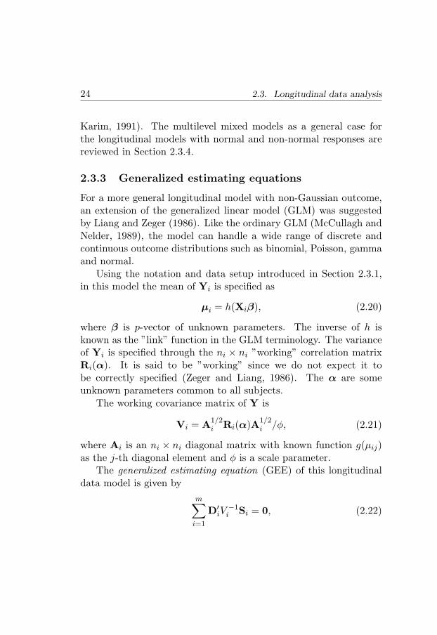
For a more general longitudinal model with non-Gaussian outcome,an extension of the generalized linear model (GLM) was suggestedby Liang and Zeger (1986). Like the ordinary GLM (McCullagh andNelder, 1989), the model can handle a wide range of discrete andcontinuous outcome distributions such as binomial, Poisson, gammaand normal.
Using the notation and data setup introduced in Section 2.3.1,in this model the mean of Yi is specified as
µi = h(Xiβ), (2.20)
where β is p-vector of unknown parameters. The inverse of h isknown as the ”link” function in the GLM terminology. The varianceof Yi is specified through the ni × ni ”working” correlation matrixRi(α). It is said to be ”working” since we do not expect it tobe correctly specified (Zeger and Liang, 1986). The α are someunknown parameters common to all subjects.
The working covariance matrix of Y is
Vi = A1/2i Ri(α)A
1/2i /φ, (2.21)
where Ai is an ni × ni diagonal matrix with known function g(µij)as the j-th diagonal element and φ is a scale parameter.
The generalized estimating equation (GEE) of this longitudinaldata model is given by
m∑
i=1
D′iV
−1i Si = 0, (2.22)

2.3. Longitudinal data analysis 25
where Di = ∂µi/∂β and Si = Yi − µi. The GEE estimator of β isthe solution of equation (2.22). Liang and Zeger (1986) studied theconsistency of the estimator and proposed an iterative procedure toestimate β.
A problem that frequently arises in longitudinal data is missingvalues. The GEE estimation is still consistent even when Ri is miss-specified provided that the missing values are completely at random(Liang and Zeger, 1986; Diggle et al., 2002). When the missing val-ues are not completely random, joint modeling of dropouts (missingvalues) and longitudinal measurements may be needed.
The approach considered here is called the population averaged(PA) models (Zeger, Liang and Albert, 1988) in which the aggre-gate response for the population is modeled. Another approach isthe subject specific (SS) models in which heterogeneity in regressionparameters is modeled. The next section considers the second ap-proach.
2.3.4 Generalized linear mixed models
The models discussed in the previous two sections can be extendedto more general class of models. Generalized linear mixed model(GLMM) is an extension of GLM by including random effects, ormore general multilevel or hierarchical structure in the model.
Rather than modeling the mean of Y as in the previous section,this model focus on modeling ui =E(Y | b) specified as
ui = h(Xiβ + Zibi), (2.23)
where b is vector of random effects with design matrix Zi. Theinverse of h is the ”link” function as in Equation (2.20). This modelis also known as subject specific (SS) in (Zeger et al., 1988). SSmodels are desirable when the response of an individual is the focusrather than the average population response.

26 2.4. Time-dependent covariates
The GEE can be used for this model as well. In the GLMMboth the link function and the random effects distribution must becorrectly specified. To use GEE for the GLMM, the marginal mo-ments µi and Vi of Equations (2.20) and (2.21) are calculated fromthe conditional moments and the random effects distribution F andsolve the GEE.
The GLMM estimation using GEE aims primarily at estimatingfixed effects and does not estimate the random component termswhich are often useful for prediction or in model diagnostic. Lately,Lee and Nelder (2001) developed hierarchical GLM that allows mod-els with any combination of GLM distribution for the response withany conjugate distribution for the random effects, structured disper-sion components, different link functions for the fixed and randomeffects and the use of quasilikelihoods in place of likelihoods for eitheror both of the mean and dispersion models.
2.4 Time-dependent covariates
2.4.1 Some useful classifications
Longitudinal or event history data has the advantage of observingthe temporal order of the outcome and covariate. The analysis ofcovariate changes may be useful in studying causal relationships. Atime-dependent covariate is a covariate that vary over time. Thissection discusses basic issues of time-dependent covariates for bothevent history and longitudinal data.
In survival analysis, Kalbfleisch and Prentice (2002, Section 6.3)classify time-dependent covariates as external and internal. Let xi(t)denote the time-dependent covariate at time t for individual i andXi(t) = xi(u); 0 ≤ u < t denote the covariate history up to time

2.4. Time-dependent covariates 27
t. For each individual i, the hazard function of (2.8) becomes
λi(t | Xi(t)) = lim∆t↓0
1
∆tP(t ≤ Ti < t + ∆t | Ti ≥ t,Xi(t)). (2.24)
An external (time-dependent) covariate Xi(t) satisfies the condi-tion
P(u ≤ Ti < u + ∆u | Ti ≥ u,Xi(u)) =
P(u ≤ Ti < u + ∆u | Ti ≥ u,Xi(t)) (2.25)
for all u, t such that 0 < u ≤ t. An equivalent condition is
P(Xi(t) | Ti ≥ u,Xi(u)) = P(Xi(t) | Ti = u,Xi(u)), 0 < u ≤ t.(2.26)
This condition implies that the future path of Xi(t) up to any timet > u is not affected by the occurrence of an event at time u.
When the conditions (2.25) or (2.26) are not satisfied, Xi(t) iscalled an internal covariate. The main consequence of internal co-variate is that the future path of the covariate is affected by theevent occurrence.
External covariates may be classified further as fixed, defined andancillary covariates. When the external covariate is fixed acrosstime, e.g., X(t) = Z, then the hazard function of (2.24) is the sameas (2.8). A defined covariate is when X(t) determined in advancedfor each individual. This covariate is usually a factor determinedin experimental study. Another example is the age of individual orcalendar time across the study. An ancillary covariate is the outputof stochastic processes that is external to the time-to-event processof the individual, such as pollution, seasonality or social-economicsconditions.

28 2.4. Time-dependent covariates
The relation between the hazard function and the survival func-tion for the external covariate is given by
S(t | X(t)) = exp
[−
∫ t
0λ(u | X(u))du
], (2.27)
which is similar to that of a time-independent covariate. The rela-tionship for the internal covariate is different to (2.27) and discussedin the next section.
In LDA, there are similar definitions for internal and external co-variates. We consider the notation in Section 2.3.1 with modification,Xij denotes the time-dependent covariate and Zij denotes the time-independent covariates. Here j represents discrete follow-up times.Adapted from econometrics terminology, in the LDA, a covariate isclassified as exogenous or endogenous (Diggle et al., 2002).
Define the history of time-dependent covariates and outcomesfor individual i up to time t as HXi(t) = Xi1, Xi2, . . . , Xit andHY i(t) = Yi1, Yi2, . . . , Yit, respectively, exogenous is defined as
f(Xit | HY i(t),HXi(t − 1),Zi) = f(Xit | HXi(t − 1),Zi), (2.28)
where f(.) represents a density or probability function of the covari-ate. When the condition (2.28) is not satisfied, HXi(t) is endogenous.
When covariates are exogenous, the future of the covariates arenot affected by the outcomes and the analysis can focus on specifyingthe dependence of Yit on Xi(t−1), Xi(t−2), . . .. Generally, the approachconsider E(Yit | Xis, s < t). For example, a GEE model with singlelagged covariate can be specified as
h(E(Yit | Xis,Zi)) = β0 + β1Xi(t−k) + β′2Zi. (2.29)
All methods and inferences discussed in Section 2.3.2 and Section2.3.3 basically can be used in the lagged model.

2.4. Time-dependent covariates 29
2.4.2 Approaches in the Cox model
The partial likelihood for the Cox model with time-dependent co-variate is similar with (2.11). The form of the Cox partial likelihoodis
L(β) =
n∏
k=1
∏
t>=0
[Yi(t) exp(β′Zk(t))∑n
j=1 Yj(t) exp(β′Zj(t))
]dNk(t)
, (2.30)
where Zj(t) is the time-dependent covariate at time t. The calcula-tion of the likelihood requires covariate values at the event times.
Typical situations in survival analysis with time dependent co-variates are illustrated in Figure 2.1. Figure 2.1(c) is a switchingtreatments time dependent covariate (Cox and Oakes, 1984, Chap-ter 8) in which subjects may change from one treatment to another.The usual method to deal with such a covariate, given that the co-variate is external, is to split the individual life time by the timewhen the covariate values change. This is easy to manage in stan-dard statistical packages that facilitate the counting process style ofinput.
Figure 2.1(b) is an example of a defined time-dependent covari-ate. For example, if the time scale used in the analysis is time sinceentering the study, a defined covariate could be the age of the in-dividuals. Of course, age has the same speed as the survival time,and their values are always available at any event time. Unlike theprevious example, it is computationally more efficient to split theindividual life times by event times.
Often, covariates are collected intermittently across the time suchthat their values are not available at the event times (Figure 2.1(a)).In this situation several methods have been proposed. These includethe last value carried forward (LVCF ) method, using the last value ofthe covariate to substitute the missing value prior to the event time.

30 2.4. Time-dependent covariates
event - outcome
covariates
(a)
*
* *
*
(b)
(c)
Figure 2.1: Time-to-event and time-dependent covariates: (a) in-termittently observed (b) defined covariate (c) switching treatmentscovariate.

2.4. Time-dependent covariates 31
Imputation methods such as two-stage estimation and smoothing canbe applied to this problem as well. In the two-stage method, a mixedmodel is fitted to the data at each event time with time-dependentcovariate as the response (Pawitan and Self, 1993; Tsiatis et al.,1995). Bruijne et al. (2001) suggested another approach using timeelapsed since the last measurement (TEL) in the Cox’s regressionmodel together with the LVCF or other methods of imputation. TheTEL can be considered as ”the age of the longitudinal measurement”in which Cox’s model that includes TEL may be better than theCox’s model with only LVCF or two-stage imputation.
More general methods based on the joint modeling of event-timesand longitudinal measurements have also been proposed (Wulfsohnand Tsiatis, 1997; Henderson et al., 2000; Lin, Turnbull, McCullochand Slate, 2002; Xu and Zeger, 2001; Tsiatis and Davidian, 2004).Basically, this model consider two linked sub-models, one for thelongitudinal measurements model and one for the event-time model.The two sub-models are joined together with a Gaussian latentprocess. Without the latent process the models become the ordi-nary separate longitudinal measurement and event-time models.
To estimate the model, a likelihood based method leading to EMalgorithms has been proposed (Wulfsohn and Tsiatis, 1997; Hen-derson et al., 2000; Lin, Turnbull, McCulloch and Slate, 2002).Other methods are based on a Bayesian approach (Faucett andThomas, 1996; Xu and Zeger, 2001; Guo and Carlin, 2004). Uti-lizing the usual connection between survival analysis and GLM, themodel can also be estimated using the GEE approach (Rochon andGillespie, 2001) and by generalized linear latent mixed models (Rabe-Hesketh, Yang and Pickles, 2001).

32 2.4. Time-dependent covariates
2.4.3 Time-dependent confounders
The notion of time-dependent confounders in epidemiology has beenrecognized at least by Robins (1986) and later in the epidemiologi-cal journals in the 90’s (see for example articles by The Cebu StudyTeam (1991); Pearce (1992); and Zohoori and Savitz (1997)). Keid-ing (1999) gave an overview of this problem in event history analysis.A time-dependent confounder, often arising in longitudinal or cohortstudies, is both a confounder and an intermediate variable. It is alsoknown as feedback models (Zeger and Liang, 1991) and related to theinternal or endogenous discussed covariates in the previous section.
To deal with time-dependent confounders in longitudinal data,we may use a method proposed by Zeger and Liang (1991). Themethod is based on GEE models allowing for both lagged responseand endogenous covariates. A more general solution with theoreticalexposition can be found in a book by van der Laan and Robins(2003).
For EHA, time-dependent confounders is closely related to in-ternal covariates. The hazard function for an internal covariate isdefined by (2.24) but conditioned on the time-dependent covariateonly up to t− (time just before t) and not further. The relation(2.27) does not hold. In fact, for survival data, the internal covari-ate requires the survival of individuals for its existence, therefore thesurvival function is always one, provided that x(t−) 6= 0. Generallythe survival function will be (Jewell and Kalbfleisch, 1996; Ander-sen, 2003)
S(t | X(t)) = E
exp
[−
∫ t
0λ(u | X(u))du
], (2.31)
where the expectation is taken with respect to the sample path X(.).The marginal survival probability at t given the past history is theaverage over the possible paths among individuals at risk for X(t).

2.4. Time-dependent covariates 33
In Cox’s regression model, care must be taken in interpretingthe estimated coefficients, since X(t) may serve as an intermedi-ate variable. However, an internal covariate is not something to beavoided, a particular kind of internal covariates known as markeror surrogate end-point have many useful applications (Jewell andKalbfleisch, 1996; Prentice, 1989).
The multiple time scales problem in the next chapter is closelyrelated to the defined covariate (Figure 2.1(b)), whereas the longi-tudinal measurement problem in Chapter 5 is closely related to theintermittently observed time-dependent covariate (Figure 2.1(a)).

34 2.4. Time-dependent covariates

Chapter 3
Analysis of Childhood
Mortality, Morbidity and
Growth
3.1 Introduction
This chapter presents some applications of event history analysis(EHA) and longitudinal data analysis (LDA) to a childhood epidemi-ological study. The Community and Health Nutrition Laboratories(CHN-RL) surveillance and the ZINAK study on zinc and iron sup-plementation in infants introduced in Chapter 1 are the two mainsources of data used in the analysis. This chapter is also meant tobe a natural background for methodological development in the laterchapters.
35

36 3.2. Mortality
3.2 Mortality
Child survival in developing countries has been investigated inten-sively, especially since the study by Mosley and Chen (1984). TheCox model for analyzing childhood mortality in developing countrieshas been employed by, among others, Trussell and Hammerslough(1983) and Pebley and Stupp (1987). Using the Community Healthand Nutrition Research Laboratories (CHN-RL) data, infant mor-tality has been investigated relating to the effects of sibling status(Wahab, Winkvist, Stenlund and Wilopo, 2001). In general, theyconcluded that boys had higher infant mortality rates than girls al-though the difference was not great. The risk for boys was evenhigher when they were born after a few siblings compared with be-ing first-born. Further study is still needed to evaluate the differentmortality pattern among boys and girls in that area.
Here, we investigated more aspects on the effect of siblings andgender on childhood mortality, taking into account clustering levelsof mother, household, community and village using EHA. Detail ofthe analysis has been reported elsewhere by Danardono (2003).
3.2.1 Data, study variables and models
Rather than considering the live births for a period of 1995 to 1996in the CHN-RL surveillance (Wahab et al., 2001) as the subjects, weconsidered all children observed since the start of surveillance on Oc-tober 1994. This scheme has an advantage in utilizing all informationavailable in the surveillance but introduces length-biased sampling(Section 1.2). Consequently, the length-biased sample selection hasto be taken into account in the analysis by using left-truncation. Af-ter excluding some twins and incomplete records, 7889 children wereavailable in the data set with 2948 of them being born after the startof the surveillance data collection.

3.2. Mortality 37
Specifically, we investigated the sibling and gender effects onmortality. The sibling factor has been pointed out as being of in-terest, in the way that it may explain the difference in care be-tween boys and girls and possible competing resources among them(Wahab et al., 2001). To study this effect, several variables wereconstructed based on gender and birth order. The sibling variable isa time-dependent covariate, a ”switching treatment” like covariate(see Figure 2.1(c) in Chapter 2).
We give one example of this variable construction. We use theterm index child to denote the child under consideration. Supposewe have information as in Figure 3.1(a). When a younger siblingwas born the value of this time dependent covariate is changed from0 to 1. We may further consider the gender of the younger siblingand categorize boy or girl rather than just 1 as the value of thistime-dependent covariate.
In Figure 3.1(a), there are two children who experienced theevents before the event times of the index child, and one child, thesibling of the index child, who has not experienced the event. Wecan construct the data suitable for event history analysis using Cox’smodel by event-time splitting (Figure 3.1(b)) or covariate-time split-ting (Figure 3.1(c)). Both constructions will lead to the same result.However, in the case of switching treatment covariate, in which thevalue of the covariate is a step function with only a few values, split-ting by covariate times is more efficient since it usually gives lesssplitting intervals than event-time splitting.
Another situation is when the index child did not enter frombirth (delayed entry or left-truncation) and the younger sibling wasborn before the entry time. In this case, there is no splitting bythe younger sibling covariate, except if the sibling dies. A similarconstruction is applied for the older sibling covariate where the valueis changed when the older sibling dies. For this analysis, we only

38 3.2. Mortality
constructed covariates for the closest sibling (one younger or oneolder sibling).
We used the Cox proportional hazards model reviewed in Sec-tion 2.2.3, i.e., the standard model of Equation (2.9) and the sharedfrailty model of Equation (2.13). We used gamma frailty to modelthe frailties. Currently, there is no general agreement about thebest frailty distribution for practical frailty modeling (Therneauand Grambsch, 2000). The Gamma distribution, however, hasbeen used in several statistical and demographical studies (Guo andRodrıguez, 1992; Sastry, 1997). To estimate the frailty term, we usedthe penalized partial likelihood approach (Therneau and Gramb-sch, 2000), available in the R survival package (Ihaka and Gentle-man, 1996; R Development Core Team, 2004).
3.2.2 Results
We obtained two hazard models for the childhood mortality: theinfant mortality (0-1 year of age) and child mortality (1-5 years ofage), presented in Table 3.1 and 3.2, respectively.
For the infant mortality hazard model, the strongest, yet unsur-prising, result is the effect of maternal education. Higher educationgave a protective effect for childhood mortality. The gender of theindex child alone was slightly a significant factor for childhood mor-tality; girls seemed to have lower risk than boys. Birth order alsoshows a significant linear effect on mortality, the risk increases withhigher birth order. The older sibling variable does not seem showany effect, the relative risk of infants (0-1 year of age) who had noolder sibling, older brother or sister are the same.
After infancy (aged 1-5 years), the effects of gender, birth orderand maternal education seem to disappear, on the other hand theeffects of siblings appear. We also examined the interaction betweengender of the index child and the gender of the older sibling as well

3.2. Mortality 39
(a) event - death
younger sibling
0
1
0 12 15 24 30
age (months)
(b)start stop status sibling
0 12 0 012 24 0 124 30 1 1
(c)start stop status sibling
0 15 0 015 30 1 1
Figure 3.1: Sibling as a time-dependent covariate: (a) The bold lineunder event-death frame is the index child, the dashed lines are otherchildren; the line under younger sibling frame is the time-depedentcovariate value; (b) splitting by event times; (c) splitting by covariatetimes.

40 3.2. Mortality
0 2 4 6 8
−10
19−
1018
−10
17−
1016
random effect variance
Log(
part
ial−
likel
ihoo
d)
95% c.i. (mother)
95% c.i. (household)
Figure 3.2: Profile likelihood for the mother and household randomeffect variance for infant mortality model.
as the younger sibling. Neither interaction was significant. Therisk of mortality is higher when the index child (boy or girl) has anolder or younger brother. The above results probably do not reflectgender difference in care, in favor of boys, since the index child withthe higher risk is either boy or girl, but it may reflect exhaustingresources when a family has a boy (or boys) that lead to childhoodmortality. The confidence intervals of the relative risks of this modelare shown in Table 3.2, under the standard model. The estimatesare rather poor with wide confidence intervals for the sibling variableand maternal education.
We also included several frailty terms that assumed to operateon a certain meaningful level. The mother frailty may capture anyunobserved variables that operate on children born from the same

3.2. Mortality 41
Tab
le3.
1:Fiv
ehaz
ard
model
sfo
rin
fant
mor
tality
(0-1
yea
rs)
Var
iable
sst
andar
dm
odel
mot
her
frai
lty
hou
sehol
dfr
ailty
com
munity
frai
lty
villa
gefr
ailty
RR
(c.i.)
RR
(c.i.)
RR
(c.i.)
RR
(c.i.)
RR
(c.i.)
Gen
der
boy
11
11
1gi
rl0.
71(0
.50-
1.01
)0.
70(0
.49-
0.99
)0.
69(0
.49-
0.98
)0.
71(0
.50-
1.01
)0.
72(0
.51-
1.01
)B
irth
order
(lin
ear)
1.16
(1.0
0-1.
35)
1.17
(1.0
1-1.
36)
1.18
(1.0
1-1.
37)
1.16
(1.0
0-1.
34)
1.16
(1.0
0-1.
34)
Mat
ernal
age
atdel
iver
y20
-29
year
11
11
1<
20ye
ar1.
72(0
.89-
3.32
)1.
76(0
.91-
3.40
)1.
79(0
.93-
3.45
)1.
69(0
.88-
3.26
)1.
70(0
.88-
3.28
)+
30ye
ar0.
95(0
.61-
1.48
)0.
98(0
.63-
1.53
)0.
99(0
.64-
1.54
)0.
97(0
.62-
1.50
)0.
96(0
.62-
1.48
)O
lder
sibling
non
e1
11
11
older
bro
ther
1.29
(0.7
2-2.
34)
1.23
(0.6
8-2.
22)
1.20
(0.6
7-2.
17)
1.29
(0.7
1-2.
32)
1.29
(0.7
2-2.
34)
older
sist
er1.
07(0
.57-
1.99
)1.
02(0
.55-
1.90
)0.
99(0
.54-
1.87
)1.
06(0
.57-
1.98
)1.
07(0
.57-
1.99
)M
ater
nal
educa
tion
12ye
ars
ofed
uca
tion
11
11
1no
educa
tion
11.5
9(3
.84-
34.9
6)11
.83
(3.9
2-35
.69)
11.9
8(3
.97-
36.1
4)11
.06
(3.6
7-33
.37)
11.4
7(3.
80-3
4.60
)6
year
sof
educa
tion
5.95
(2.1
7-16
.33)
6.07
(2.2
1-16
.64)
6.08
(2.2
2-16
.69)
5.8
(2.1
1-15
.89)
5.96
(2.1
7-16
.34)
9ye
ars
ofed
uca
tion
4.63
(1.5
6-13
.72)
4.73
(1.5
9-14
.02)
4.76
(1.6
1-14
.11)
4.59
(1.5
5-13
.61)
4.63
(1.5
6-13
.74)
Var
iance
ofra
ndom
effec
t1
mot
her
2.13
5(0
.041
)hou
sehol
d3.
074
(0.0
04)
com
munity
0.10
3(0
.319
)villa
ge0.
054
(0.3
34)
1T
he
esti
mat
edva
rian
ceof
random
effec
tsan
dth
ep-v
alue
ofth
eLRT

42 3.2. Mortality
Tab
le3.2:
Fiv
ehazard
models
forch
ildm
ortality(1-5
years)
Variab
lesstan
dard
model
moth
erfrailty
hou
sehold
frailtycom
munity
frailtyvillage
frailtyR
R(c.i.)
RR
(c.i.)R
R(c.i.)
RR
(c.i.)R
R(c.i.)
Gen
der
boy
11
11
1girl
0.97(0.46-2.07)
0.97(0.46-2.07)
0.97(0.46-2.07)
0.97(0.46-2.07)
0.96(0.45-2.04)
Birth
order
(linear)
0.87(0.58-1.31)
0.87(0.58-1.31)
0.87(0.58-1.31)
0.87(0.58-1.31)
0.87(0.58-1.30)
Matern
alage
atdelivery
20-29year
11
11
1<
20year
1.31(0.19-8.90)
1.31(0.14-12.10)
1.31(0.14-12.1)
1.31(0.14-12.10)
1.33(0.14-12.28)+
30year
0.84(0.38-1.88)
0.84(0.34-2.06)
0.84(0.34-2.06)
0.84(0.34-2.06)
0.85(0.35-2.09)
Old
ersib
ling
non
e1
11
11
older
broth
er11.46
(2.64-49.8)11.46
(2.01-65.23)11.46
(2.01-65.23)11.46
(2.01-65.23)11.57(2.03-65.82)
older
sister6.34
(1.26-32.01)6.34
(1.03-38.87)6.34
(1.03-38.87)6.34
(1.03-38.87)6.35(1.04-38.97)
You
nger
siblin
gnon
e1
11
11
younger
broth
er4.86
(1.44-16.45)4.86
(1.45-16.31)4.86
(1.45-16.31)4.86
(1.45-16.31)4.88(1.46-16.38)
younger
sister1.2
(0.16-9.01)1.2
(0.15-9.65)1.2
(0.15-9.65)1.2
(0.15-9.65)1.17
(0.14-9.39)M
aternal
education
12years
ofed
ucation
11
11
1no
education
2.03(0.12-33.78)
2.03(0.13-32.95)
2.03(0.13-32.95)
2.03(0.13-32.93)
1.93(0.12-31.33)6
yearsof
education
5.02(0.68-37.29)
5.02(0.67-37.67)
5.02(0.67-37.67)
5.02(0.67-37.67)
4.95(0.66-37.12)9
yearsof
education
2.07(0.19-22.09)
2.07(0.19-22.92)
2.07(0.19-22.92)
2.07(0.19-22.92)
2.07(0.19-23.00)V
ariance
ofran
dom
effect
1
moth
er≈
0≈
1hou
sehold
≈0
≈1
comm
unity
0.0050.947
village
0.1840.423
1The
estimated
variance
ofran
dom
effects
and
the
p-valu
eof
the
LRT

3.2. Mortality 43
mother, such as genetic factors and maternal competence. At thehousehold level, family size, socio-economic status and housing con-dition may be captured by household frailty term. At the broadercoverage of level, community and village level were also included.These terms will account for the possible effects of infrastructure,climate, and other environmental factors within the community; andinstitutional effect within the village.
Figure 3.2 shows the profile likelihood for the mother and house-hold frailty term. The 95% confidence interval is constructed byreferencing a horizontal line 3.84/2 units below the maximum log-partial likelihood. The reference line is obtained by assuming that2×(the difference in likelihood) has Chi-square distribution with onedegree of freedom. The maximum log likelihood of the householdfrailty model is -1015.48, which corresponds to the value 3.074 ofthe estimated random effect variance, and -1017.43 for the motherfrailty effect, which corresponds to the estimated random effect vari-ance of 2.14. The intervals range from 0.63 to 7.70 for the householdfrailty, and 0.07 to 6.38 for the mother frailty. In fact, no intervalcover zero value of the random effect variance, suggesting that thehousehold and mother frailty are important. For community andvillage frailty, the 95% confidence intervals cover the zero value ofthe random effect variance, indicating that the community and vil-lage frailty are not important. This confirms the results of Table3.1, in which household and mother frailty are important, whereascommunity and village frailty are not.
High household frailty effect indicates that housing condition,socio-economic status and other household level factors are moreimportant than other factors that operate at mother, community orvillage level. The mother’s frailty effect was lower than the house-hold, probably because some of the important maternal variablesfor childhood mortality have been accounted for in the model, suchas maternal education and maternal age at delivery, whereas none

44 3.3. Morbidity: surveillance data
of household’s variables have been included. It is suggested thathousehold factor variables should be included for further studies.
Similar to the infant mortality model, the estimated parametersin the child mortality models with frailty do not differ from thestandard model (Table 3.2).
The general conclusion regarding the sibling and gender factors isthat there was no evidence of gender difference reflected as differencein care between boys and girls in Purworejo district, Indonesia thatmay lead to mortality. This finding is in accord with the previousresearch (Wahab et al., 2001) and the general trend of the narrow-ing gaps in many aspects between boys and girls in the Indonesiansociety (Kevane and Levine, 2003). There is, however, an indicationthat having brother(s) may lead to higher risk of child mortality.
3.3 Morbidity: surveillance data
Because of its importance, childhood morbidity has been investi-gated by many researchers from diverse disciplines such as publichealth, biomedicine and social science. Two common diseases inchildhood, diarrhea and respiratory infection, remain to be the mostimportant causes of deaths among children (Rice, Sacco, Hyder andBlack, 2000; Black, Morris and Bryce, 2003; UNICEF, 2003). In In-donesia, especially in the CHN-RL area, several studies related tochildhood morbidity have been conducted. Machfudz (1998) con-ducted a study on the effect of morbidity (diarrhea and respiratoryinfection) on the change of the mid-upper-arm circumference in chil-dren under five years of age. Danardono (2000) studied the multileveleffects at community level, household level and individual level forthe case of diarrhea disease. Wibowo (2000) evaluated the influenceof nutritional status on morbidity (diarrhea and respiratory tractinfection) among infants.

3.3. Morbidity: surveillance data 45
We presented the application of EHA for analyzing two commonand important childhood diseases, diarrhea and respiratory infectionin the CHN-RL surveillance area. We demonstrated the use of var-ious time scales to respond to research questions of interest. As inthe previous section, the detail of the analysis in this section hasbeen reported elsewhere by Danardono (2003).
3.3.1 Data, study variables and models
We utilized the CHN-RL morbidity surveillance for this analysis.The surveillance used the two-week recall questionnaire to collectinformation on childhood morbidity at the day of visit and 14 daysbackward and related variables. This type of questionnaire has beenwidely used for morbidity records, for instance in the Demographicand Health Surveys (DHS) in many countries, including Indonesia(CBS, NFPCB, MOH and MI, 1998).
The variables of interest are gender of the child, maternal ed-ucation and maternal age (at the time of illness), sibling variables(as in the childhood mortality models in the previous section) andbreastfeeding. Individual frailty effects as well as environmental andinstitutional frailty effects are also investigated. To ensure that in-formation on the breastfeeding variable is available, cohort data fromFebruary 1995 until June 1998 were used with 2804 children availablein the data set.
To analyze the data, we need to construct the data set intocounting process style of input (start, stop], event. The processis straightforward but tedious, and computer demanding when thedata set is large and includes time dependent covariates. Table 3.3represents the data layout for the morbidity study. The observationcolumn is the information obtained by the two-week recall ques-tionnaire. The start, stop, event columns are constructed by theobservation column and visit column. For instance, child with ID
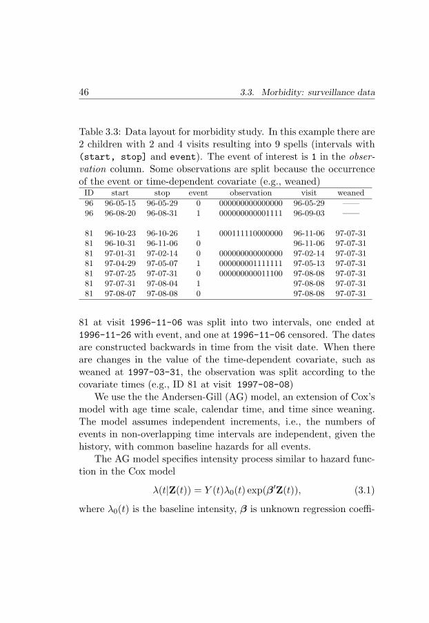
46 3.3. Morbidity: surveillance data
Table 3.3: Data layout for morbidity study. In this example there are2 children with 2 and 4 visits resulting into 9 spells (intervals with(start, stop] and event). The event of interest is 1 in the obser-vation column. Some observations are split because the occurrenceof the event or time-dependent covariate (e.g., weaned)ID start stop event observation visit weaned
96 96-05-15 96-05-29 0 000000000000000 96-05-29 ——96 96-08-20 96-08-31 1 000000000001111 96-09-03 ——
81 96-10-23 96-10-26 1 000111110000000 96-11-06 97-07-3181 96-10-31 96-11-06 0 96-11-06 97-07-3181 97-01-31 97-02-14 0 000000000000000 97-02-14 97-07-3181 97-04-29 97-05-07 1 000000001111111 97-05-13 97-07-3181 97-07-25 97-07-31 0 000000000011100 97-08-08 97-07-3181 97-07-31 97-08-04 1 97-08-08 97-07-3181 97-08-07 97-08-08 0 97-08-08 97-07-31
81 at visit 1996-11-06 was split into two intervals, one ended at1996-11-26 with event, and one at 1996-11-06 censored. The datesare constructed backwards in time from the visit date. When thereare changes in the value of the time-dependent covariate, such asweaned at 1997-03-31, the observation was split according to thecovariate times (e.g., ID 81 at visit 1997-08-08)
We use the the Andersen-Gill (AG) model, an extension of Cox’smodel with age time scale, calendar time, and time since weaning.The model assumes independent increments, i.e., the numbers ofevents in non-overlapping time intervals are independent, given thehistory, with common baseline hazards for all events.
The AG model specifies intensity process similar to hazard func-tion in the Cox model
λ(t|Z(t)) = Y (t)λ0(t) exp(β′Z(t)), (3.1)
where λ0(t) is the baseline intensity, β is unknown regression coeffi-

3.3. Morbidity: surveillance data 47
cients, Z(t) is vector of covariate, possibly time-dependent and Y (t)is zero-one at-risk process. Unlike the Cox model for survival data,Y (t) in the AG model is not absorbed to zero when an event occursbut alternates between zero and one depending on the event process.The purpose of counting process style of input (start, stop], eventmentioned above is to specify the Y (t).
In the analysis we used the AG model with three different timescales, i.e., age, time since the start of the surveillance, and timesince weaning.
3.3.2 Age time scale
Respiratory infection and diarrhea, as well as many other childhooddiseases are usually age dependent. Choosing age as the time scaledoes not allow age itself to be in the model, but we can check thedependency by looking at the hazard plot. Figure 3.3 shows the plotof the hazards for both diseases. The hazard plots are smoothedby the Epanechnikov kernel, with a bandwidth of 10 months chosenby visual inspection, and plotted over the monthly crude hazardrates (the shaded barplot). The visual inspection is of course notan optimal method for choosing a bandwidth, compared with themethod suggested by Andersen et al. (1993), but it is useful enoughfor exploratory purposes. The cumulative hazards of both diseasesare almost linearly increasing. The estimated hazards show that thehazard might be associated with age, and around 12 months of agecould be the highest peak of both diseases.
Table 3.4 gives the result for diarrhea. Increasing maternal ageseems to be associated with increasing the risk. The breastfeedingvariable has a rather significant contribution to the model wherethe never breastfed children had the highest risk as compared to theother categories. Maternal education and sibling variables did notshow any significant contribution in the model.

48 3.3. Morbidity: surveillance data
02
46
8
age (months)
cum
ulat
ive
haza
rd
0 5 10 15 20 25 30 35 40
Respiratory Infection
0.0
0.4
0.8
1.2
age (months)
cum
ulat
ive
haza
rd
0 5 10 15 20 25 30
Diarrhea
0.0
0.1
0.2
0.3
0.4
0.5
age (months)
haza
rd
0 5 10 15 20 25 30 35 40
0.00
0.04
0.08
age (months)
haza
rd
0 5 10 15 20 25 30
Figure 3.3: The cumulative hazard and hazard plot of childhoodrespiratory infection and diarrhea by age.

3.3. Morbidity: surveillance data 49
Table 3.4: Hazard model for diarrhea, age time scale
Variables Relative risk (c.i.) p-value p-valueLRT1 Non-prop2
Gender 0.298boy 1 (reference)girl 1.14 (0.87-1.51) 0.581
Maternal education 0.174non-educated 1 (reference)educated 1.58 (0.8-3.14) 0.784
Breastfeeding status 0.088breastfed 1 (reference)weaned 1.09 (0.69-1.73) 0.179never breastfed 2.07 (1.04-4.11) 0.260
Maternal age (years) <0.00115-19 1 (reference)20-24 1.40 (0.75-2.60) 0.55525-29 1.70 (0.95-3.03) 0.24730-34 1.14 (0.59-2.22) 0.73135+ 1.66 (0.86-3.21) 0.383
Older sibling 0.640none 1 (reference)brother 0.84 (0.57-1.24) 0.902sister 0.91 (0.62-1.33) 0.846
Younger sibling 0.988none 1 (reference)brother 1.12 (0.29-4.39) 0.630sister 0.99 (0.27-3.67) 0.9911Likelihood ratio test 2Non-proportionality test, global p-value=0.89

50 3.3. Morbidity: surveillance data
The frailty effects of this hazard model for diarrhea are all signifi-cant, with the value of 1.273, 1.229, 1.237, 0.614, 0.350 for individual,mother, household, community and village frailty, respectively. Theestimated coefficients in the frailty models are only slightly differ-ent to the estimated coefficients of the standard model (Table 3.4),which may not give any further important information. However, thesignificant frailty effect of these frailty models indicate the existenceof unobserved heterogeneity in the individual, mother, household,community and village groups which may need to be investigatedfurther.
For the respiratory infection, the maternal age has a similar pat-tern to the diarrhea models as well as for the sex and sibling variables.Contrary to the diarrhea model, maternal education gave significantcontribution to the model whereas the breastfeeding variables didnot. The frailty effects for the respiratory infection model were alsofound to be important in the models.
For both hazards models of respiratory infection and diarrhea,there is no evidence of non-proportionality, as indicated by the globalp-values test for non-proportionality (large values) and the p-valuesfor each coefficient in both models. All necessary interactions, suchas maternal education and breastfeeding, have also been checked andtaken care of.
3.3.3 Calendar time
We used other time scales than age to allow age as a time dependentcovariate in the model. One possible choice is the time since thestart of the surveillance (February 1995).
Figure 3.4 shows the cumulative hazards and hazard as a func-tion of time since the start of the surveillance where time is convertedback to a calendar time. Against time, the hazard of respiratory in-fection is always higher than diarrhea. The highest peak of respira-

3.3. Morbidity: surveillance data 510
24
68
cum
ulat
ive
haza
rd
Feb95 Aug95 Feb96 Aug96 Feb97 Aug97 Feb98
Respiratory infection
Diarrhea
01
23
45
haza
rd
Feb95 Aug95 Feb96 Aug96 Feb97 Aug97 Feb98
Respiratory infection
Diarrhea
Figure 3.4: The cumulative hazards and hazards plot of childhoodrespiratory infection and diarrhea by calendar time.
tory infection and diarrhea incidence seemed to be in April-June, thetransition period from the rainy to the dry season; and in September-October, the transition from the dry to rainy season. There was alsoa long dry season in 1997 and an economic crisis that might havecaused the peak incidence in that year.
Table 3.5 shows the hazards model for respiratory infection. Thechildren’s age variable is significantly associated with the risk of de-veloping respiratory infection. The highest risk for respiratory infec-tion is in the 6-23 (months) age group. The conclusion is the samefor maternal education and maternal age as in the model using agetime scale. The other variables have a similar pattern to the mod-els using age as the time scale. The pattern is also similar for thediarrhea models.
Also similar to the age time scale models, introducing frailty did

52 3.3. Morbidity: surveillance data
Table 3.5: Hazards model for respiratory infection, calendar time
Variables Relative risk (c.i.) p-value p-valueLRT1 Non-prop2
Gender 0.984boy 1 (reference)girl 0.99 (0.91-1.10) 0.135
Age of the child (months) <0.0010-5 1 (reference)6-23 1.83 (1.61-2.07) 0.26724+ 1.51 (1.21-1.90) 0.722
Maternal education 0.013no education 1 (reference)6 yrs of education 1.33 (1.04-1.70) 0.1689 yrs of education 1.29 (0.99-1.69) 0.14512 yrs of education 1.42 (1.09-1.85) 0.259
Maternal age (years) <0.00115-19 1 (reference)20-24 1.29 (1.05-1.58) 0.30325-29 1.30 (1.04-1.61) 0.36730-34 1.15 (0.92-1.45) 0.46135+ 1.32 (1.04-1.67) 0.656
Breastfeeding status 0.674breastfed 1 (reference)weaned 1.01 (0.87-1.18) 0.725never breastfed 0.84 (0.55-1.28) 0.595
Older sibling 0.641none 1 (reference)brother 0.98 (0.85-1.12) 0.560sister 0.94 (0.82-1.08) 0.458
Younger sibling 0.480none 1 (reference)brother 0.98 (0.57-1.68) 0.661sister 1.32 (0.85-2.05) 0.9221Likelihood ratio test 2Non-proportionality test, global p-value=0.93

3.3. Morbidity: surveillance data 53
not change the estimated coefficients for both respiratory infectionand diarrhea models, but the frailty variance was quite significantindicating unobserved heterogeneity in the data. Neither model vio-lates the proportionality assumption of the Cox proportional hazardmodel according to the non-proportionality test.
3.3.4 Time since weaning
The protective effect of breastfeeding for childhood illness is wellknown and has been investigated by many authors, see for exam-ple Bhandari, Bahl, Mazumdar, Martines, Black, Bhan and InfantFeeding Study Group (2003) and references therein. In this section,the aim is to demonstrate the use of time since stop breastfeeding asan alternative time scale, for investigating the effect of breastfeedingon childhood morbidity. The breastfeeding definition in this sectionis simply based on the questionnaire on health status, breastfeedingand feeding practice and does not include breastfeeding pattern, suchas exclusive breastfeeding and frequency of breastfeeding. The per-centage of breastfed children is quite high in the surveillance area,about 98%, which is similar to the national figure of 96% (CBSet al., 1998). The median duration of breastfeeding is relativelylong at 24.1 months which is also close to the national figure of 23.9months.
The weaned age or the duration of breast feeding is one of thevariables of interest. This variable is a time independent covariatethat is fixed since the weaned time. Age of the child is also includedas a time dependent covariate.
Table 3.6 gives the hazards model for respiratory infection. Theweaned age is significant in the model. Although the differences ofthe effects between weaned age category are not huge, the longerweaned age seems to give a protective effect against respiratory in-fection.

54 3.3. Morbidity: surveillance data
Contrary to the previous models (with age and calendar timescale), the effect of maternal education is weak and leads to a differ-ent direction. The maternal age has similar pattern to the previousmodels. As with the previous models, there is no evidence of genderand sibling effect in this model.
The frailty effects are significant but do not change the generalconclusion of the model (the estimated coefficients). In this model,there is no indication of violating the non-proportionality assump-tion.
The hazards model for diarrhea generally gives similar results asfor respiratory infection. Here, the results are presented only forthe weaned age. The variable has fewer categorizations than forrespiratory infection because of the fitting problem. The relativerisks with confidence intervals are 0.97 (0.25-3.76), 0.53 (0.13-2.13)for weaned age group 6-12 and 12+ months (the reference is 0-5
months) and has a p-value (LRT) of 0.607.The frailty effects do not change the coefficient estimation of the
hazards model for diarrhea. In fact, no frailties effects for diarrheaare significant. It may really show that there are no unobservedfactors for the risk of diarrhea or no difference in risk in these groupsor clusters (individual, mother, household, community and village).However, it is also possible that the number of observations is notlarge enough to show the frailty effects.
In general, the analysis concludes that children aged 6-23 months,or aged around one year of age, are prone to develop respiratory in-fection and diarrhea and there is a pattern of seasonality in bothdiseases. Maternal education is important. Surprisingly, the risk ofthe children developing the diseases are higher for the higher edu-cated mothers. As in the mortality study, there is no evidence ofgender and sibling’s effect.

3.3. Morbidity: surveillance data 55
Table 3.6: Hazards model for respiratory infection, time since wean-ing
Variables Relative risk (c.i.) p-value p-valueLRT1 Non-prop2
Gender 0.123boy 1 (reference)girl 1.22 (0.95-1.58) 0.925
Weaned age(months) 0.0400-4 1 (reference)5-6 0.48 (0.18-1.32) 0.9047-12 0.97 (0.55-1.74) 0.31413+ 0.58 (0.33-1.04) 0.431
Age of the child (months) 0.6840-5 1 (reference)6-23 1.41 (0.59-3.34) 0.74724+ 1.35 (0.52-3.51) 0.516
Maternal education 0.341no education 1 (reference)6 yrs of education 0.84 (0.41-1.7) 0.1139 yrs of education 0.98 (0.47-2.12) 0.19112 yrs of education 0.88 (0.42-1.86) 0.197
Maternal age 0.01815-19 1 (reference)20-24 2.44 (1.03-5.76) 0.85125-29 3.23 (1.36-7.68) 0.55130-34 2.32 (0.94-5.74) 0.56435+ 2.36 (0.93-5.97) 0.800
Older sibling 0.567none 1 (reference)brother 0.84 (0.59-1.2) 0.794sister 0.84 (0.58-1.21) 0.688
Younger sibling 0.495none 1 (reference)brother 0.77 (0.36-1.65) 0.507sister 1.26 (0.73-2.16) 0.6331Likelihood ratio test 2Non-proportionality test, global p-value=0.86

56 3.4. Morbidity: trial data
3.4 Morbidity: trial data
Deficiencies of iron and zinc often coexist and cause growth faltering,delayed development and increased morbidity from infectious dis-eases during infancy and childhood (Lind, 2004, Paper V). Therefore,combined iron and zinc supplementation may be a logical preventionstrategy.
To investigate the effect of the supplementations, a community-based, randomized, double-blind, controlled trial, the ZINAK study,was conducted from July 1997 to May 1999 in the CHN-RL area,Purworejo, Indonesia. The subjects are different to the children inthe surveillance morbidity discussed in the previous section.
This section demonstrates the use of EHA for morbidity analysisin the ZINAK data. Unlike the morbidity analysis in the previoussection, here, we have continuous data collection in which variousanalyses rather than only AG-model are possible to be performed.We considered respiratory infection as the event of interest. Togetherwith infant growth analysis in the next section, this section servesas a background problem for Chapter 5.
3.4.1 Data, study variables and models
The ZINAK study was conducted from July 1997 to May 1999 inthe CHN-RL surveillance area, Purworejo, Indonesia. Healthy andsingleton infants, aged less than six months were recruited. Afterassessing their eligibility, 680 infants were randomized into one offour treatments: iron, zinc, iron+zinc or placebo from 6 to 12 monthsof age (180 days of supplementation). More detailed description ofthe design and data collection is reported by Lind (2004). There areseveral outcomes of interest, biochemical outcomes (iron and zincconcentration in the blood), infants growth (anthropometry), infants

3.4. Morbidity: trial data 57
development (mental, psychomotor development) and morbidities.Here, we consider respiratory infection as the outcome of interest.
Morbidity information was obtained by visitation every third day.Field workers asked the parents or guardians regarding the com-pliance to supplementation as well as information on symptoms ofillness for the day of visit and for the two days preceding the visit.
Among 680 infants, 666 completed supplementations and someof them dropped out. It may be necessary to consider the drop-outin the analysis since all of them were related to the supplementationas reported by Lind (2004). However, at this moment we analyze thecompleted records only according to intent-to-treat analysis. Covari-ates under consideration, other than the treatment itself, are genderand maternal education.
We used the AG model with age as the time scale as in theprevious section (Equation (3.1)). Additionally, we used gap-timeor sojourn time also as an alternative time scale. The gap-timeis defined as the time since entry or previous event. When bothmodels give similar results, we can safely assume a renewal processand consider a constant baseline hazard.
As in the previous section, we may actually use calendar time aswell since morbidity may have a strong seasonal pattern. Howevergiven the rather short period of observation time (six months) andthat most of the children entered the study at almost the same time,using calendar time and age is almost identical. However, when wewant to model the morbidity with growth, which depends on agerather than calendar time, the age time scale has a clear advantageto calendar time.
3.4.2 Results
Tables 3.7 and 3.8 give the result of hazard model using the AGmodel and gap-time model. They are actually quite similar in their

58 3.4. Morbidity: trial data
Table 3.7: Hazards model for respiratory infection using the Ander-sen Gill model, ZINAK study
Variables Risk ratio (c.i.) p-value p-valueLRT1 Non-prop2
Gender 0.044boy 1 (reference)girl 0.91 (0.83-1.00) 0.308
Supplementation 0.411placebo 1 (reference)zinc 1.00 (0.88-1.14) 0.805zinc+iron 0.91 (0.79-1.03) 0.235iron 0.97 (0.85-1.11) 0.723
Maternal Education <0.001no-education 1 (reference)6 years 0.84 (0.64-1.10) 0.1339 years 0.70 (0.53-0.92) 0.42712 years or more 0.46 (0.29-0.75) 0.1021Likelihood ratio test 2Non-proportionality test, global p-value=0.177
risk ratio and p-value of the likelihood ratio test. Assuming constantbaseline hazards will give the same result. The raw and smoothedhazard function in Figure 3.5 also indicated a constant hazard duringperiod of 6 to 12 months of age.
Looking at the estimates, there is no pronounced effect of thesupplementation to respiratory infection which confirms the resultby Lind (2004) in which Poisson regression was used. This result alsoreiterates the importance of maternal education as it has been foundin the respiratory infection models using surveillance data (Section3.3). Here, the direction of the maternal education is different tothat of surveillance data. Higher education seemed to have protec-tive effect on respiratory infection. The infants’ gender was rathersignificant with girls having a lower hazard than the boys.

3.4. Morbidity: trial data 59
Table 3.8: Hazards model for respiratory infection using the gap-timemodel, ZINAK study
Variables Risk ratio (c.i.) p-value p-valueLRT1 Non-prop2
Gender 0.051boy 1 (reference)girl 0.91 (0.83-1.00) 0.014
Supplementation 0.474placebo 1 (reference)zinc 1.01 (0.89-1.15) 0.172zinc+iron 0.91 (0.80-1.04) 0.791iron 0.98 (0.86-1.11) 0.652
Maternal Education <0.001no-education 1 (reference)6 years 0.85 (0.65-1.12) 0.4849 years 0.72 (0.54-0.95) 0.17612 years or more 0.50 (0.31-0.80) 0.8831Likelihood ratio test 2Non-proportionality test, global p-value=0.101
age (months)
haza
rd
0.0
0.1
0.2
0.3
0.4
0.5
5 6 7 8 9 10 11 12 13
Figure 3.5: Raw and smoothed hazard plot of childhood respiratoryinfection by age.

60 3.5. Infant growth
The other purpose of this analysis, aside from demonstrating theapplication of EHA, is to give a background for the problem of an-alyzing EHA together with longitudinal measurements in Chapter5. It is well known that nutrition, growth and morbidity are closelyrelated (Scrimshaw, 2003). Therefore, evaluating supplementationon both growth and morbidity simultaneously may give less biasthan analyzing the two outcomes separately. Although it also hasbeen reported briefly that anthropometrical status was not associ-ated with the incidence of infectious disease (Lind, 2004), a morecareful analysis may be needed.
3.5 Infant growth
Infant growth indicators such as weight, length, knee-heel, mid-upperarm circumference are another outcome of interest collected in theZINAK study. Obviously, the type of outcomes is not a time-to-event data but ordinary continuous data. We presented the use ofLDA to analyze such data, taking weight as the outcome of interest.Also, together with the morbidity analysis in the previous sectionthis section serves as a background problem for Chapter 5.
Measurements of the weight were performed every month.Weight measurements before the period of trial were also availablefor most of the children. Figure 3.6 shows the children’s weightby age with smoothing lines. During the trial period from 6 to 12months of age, a linear model for this weight growth curve may besufficient. However, weight growth is very individually developed inwhich the between individual variance is usually large. Therefore,employing the linear random effects model reviewed in Section 2.3.2is more suitable to the weight data than the ordinary linear model.

3.5. Infant growth 61
0 5 10 15
24
68
1012
age (months)
wei
ght (
kgs)
Figure 3.6: The children’s weight across age. The greyed points de-note the actual measurements of weight; the line denotes the smooth-ing splines of the weight measurements; the dashed line denotes thereference population (CDC 2000 growth charts); and the two verticallines denote the starting and ending point of the trial.

62 3.5. Infant growth
Table 3.9: Growth curve model for weight using random effect andordinary linear model, ZINAK study
Variables Random effect model linear model
Intercept 6.37 (5.88,6.86) 6.38 ( 6.11, 6.65)Age 0.17 (0.17,0.18) 0.17 ( 0.15, 0.19)Gender
boy (reference)girl -0.54 (-0.68 ,-0.40) -0.54 (-0.61,-0.48)
Supplementationplacebo (reference)zinc 0.02 (-0.18 , 0.22) 0.08 (-0.01, 0.16)zinc+iron 0.01 (-0.19 , 0.21) 0.02 (-0.07, 0.10)iron 0.01 (-0.19 , 0.21) 0.03 (-0.06, 0.12)
Maternal Educationno-education (reference)6 years 0.20 (-0.28 , 0.68) 0.19 (-0.02, 0.40)9 years 0.31 (-0.18 , 0.79) 0.30 ( 0.09, 0.51)12 years or more 0.26 (-0.41 , 0.94) 0.27 (-0.03, 0.57)
Illness days -0.53 (-0.64 ,-0.41) -1.12 (-1.57,-0.67)
Random effectsd(Intercept) 0.993 (0.923,1.064)sd(Age) 0.065 (0.061,0.070)corr(Intercept,Age) -0.617 (-0.860,-0.430)
The model for weight is
yi = Xiβ + Zbi + ǫi, i = 1, . . . , N,
bi ∼ N(0,Σ), ǫi ∼ N(0, σ2I), (3.2)
where yi is the weight measurements on child i and N is the num-ber of children, bi is vector of random effects, Xi and Zbi are thecovariates for the fixed and random effects, respectively.
Table 3.9 shows the results of fitting the weight models using a

3.5. Infant growth 63
random effects model and also the ordinary linear model for compar-ison. The age and illness-days covariates are measured as continuousvariables while the rest are categorical. Illness days is the numberof days with illnesses (symptoms) from the previous measurementstime up to the current measurement time, as a proxy variable forthe effect of duration of illness.
The random effects model has two parts, the fixed part (upperpart of the column variables) and the random part (the lower one).First, we look at the random effects which correspond to the standarddeviation and correlation of intercept and age (the bi in model (3.2)).They were found to be significantly different from zero, as indicatedby their intervals which do not include zero. The result confirms theassumption that weight growth is quite individually developed.
Now we look at the fixed part (β in model (3.2)) and comparethe estimates with that of the ordinary linear model. The estimatedcoefficients of the two models are quite similar except for the illness-days. The confidence intervals from the random effect model aregenerally wider than that from the ordinary linear model. Thereseemed to be no effect of supplementation on the weight. The pro-nounced effects were gender, age and illness-days. We have checksome interactions as well and we found that there was no interactionbetween supplementation and illness-days.
As comparisons, we also performed two alternative analyses forthe weight longitudinal measurements. The first one is an analysiswith WAZ (weight-for-age z-score) instead of weight. The WAZ isa standardized value of the weight compared to a reference popu-lation. We used the CDC 2000 reference population (Kuczmarski,Ogden and Guo, 2002) which was also used by Lind (2004) (see thedashed line in Figure 3.6). The age and gender variables were impor-tant, similar to the weight random effect model of Table 3.9, but thedirection of the estimated regression coefficients was reversed. Theestimated 95% confidence intervals were (-0.22, -0.206) and (0.00,

64 3.6. Remarks
0.33) for age and girl, respectively. This indicates growth decreasingcompared to the growth of the CDC 2000 and the boys seemed tosuffer more than the girls. There is no different in conclusion for thesupplementation, maternal education and illness days.
The second one is an analysis using weight velocity. The weightvelocity for a certain age of individual is the weight difference be-tween the current weight and the previous measurement weight di-vided by the length of time from the previous measurement age tocurrent age. We used the ordinary linear model as the random effectpart did not show any significant contributions. The age and illnessdays still show a large effect as in the weight models. The gendereffect, however, disappeared. As in the weight models, supplementa-tion did not show any significant effect in this weight velocity model.
In conclusion, there is a general growth decrease for children inthe study compared to the standard reference population, but thesupplementation did not seem to affect the growth. It is also ofinterest to investigate the growth model in relation to time-to-eventmorbidity data. We will discuss this problem in Chapter 5.
3.6 Remarks
We have demonstrated the application of EHA and LDA to ana-lyze data from childhood health studies. There are two points ofmethodological interest emerging from the applications.
In EHA, sometimes we face more than one competing time scale.For instance, we may use calendar time instead of age in the mor-bidity model of Section 3.3. Age-period or age-period-cohort modelis another situation in which more than one time scale is involved.The problem of multiple time scales will be discussed in the nextchapter.
Important statistical issues in the ZINAK study is that the out-

3.6. Remarks 65
comes of interest may actually interact with each other and analyzingthem separately may give biased results. Specifically, the interest ison the joint analysis of time-to-event and longitudinal measurementsoutcomes. Comparison of approaches and further analysis of ZINAKrespiratory infection and growth data will be presented in Chapter 5.

66 3.6. Remarks

Chapter 4
Multiple Time Scales
4.1 Introduction
Time is indispensable in event history analysis. Although time maybe just a proxy measure for other influences of the events (Berzuiniand Clayton, 1994b), time is the most readily available measurementand easy to utilize for comparison and generalization. For example,in epidemiology, age is the most often used time scale since it re-flects cumulative damage that causes mortality, whereas, in clinicalstudies, time since diagnosis may be more important. This chapterconsiders the problem of choosing an appropriate baseline time scaleand modeling dual time scales.
The choice of time scale is driven by the research question of thestudy. However, in the absence of knowledge about the importanceof time scales, we may have to consider all relevant time scales. Inan epidemiological surveillance study, it is common to perform anexploratory study to identify new emerging risk factors. One way ofexploring the factors is by investigating several relevant time scales.In general, the choice of relevant time scales in epidemiology or ob-
67

68 4.1. Introduction
servational studies is more difficult than in clinical studies (Liestøland Andersen, 2002).
Farewell and Cox (1979) and Oakes (1995) suggested to choose abasic time scale that accounts for as much as the variation as possi-ble. Duchesne (1999) and Duchesne and Lawless (2000) introducedthe concept of ideal time scale. However, their focus is on the us-age variable (such as mileage, asbestos exposure, etc.), as the otherscale rather than the multiple origins problem, as considered in thisthesis. Multiple time scales have been considered in the multistatemodel as well. Jones and Crowley (1992) and Commenges (1999)considered the problem of multiple time scales under the Markovand semi-Markov models. Ng and Cook (1997) developed a randomeffects model that includes piecewise constant formulations. Ander-sen and Keiding (2002) suggested a practical approach to choosinga basic time scale in the Cox model.
The piecewise constant hazards and discrete time models are theusual approaches to the multiple time scales problem, if we wantto treat multiple time scales symmetrically (Keiding, 1990; Berzuiniand Clayton, 1994b). Those approaches utilize the relation betweenPoisson regression and Cox’s proportional hazards model. Efron(2002) considered the discrete time approach to develop a two-wayproportional hazards model and decomposed the hazards multiplica-tively for a dual time scales problem.
In the Cox model, other time scales (than the basic time scale)can be considered as a defined time-dependent covariate (see Section2.4.1). Therefore, Cox models with a time-dependent approach, suchas a time-dependent covariate and time-dependent strata, can beused for multiple time scales modeling.
In this chapter, procedures to choose a basic time scale in Cox’sregression model are proposed. For the dual time scales problem,the connection between piecewise constant hazards and the time-

4.2. The choice of relevant time scales 69
dependent approach is discussed. Quantitative comparisons are per-formed through simulation.
4.2 The choice of relevant time scales
The multiple time scales problem considered here is basically a mul-tiple time origins problem with time equal to ordinary clock time.The nature of the problem is different from the usual multivariatesurvival such as bivariate survival in twin studies or pairs of humanorgan studies. In the multiple time origins problem, see the Lexisdiagram in Figure 4.1(a), movement of time scale pairs is in the samedirection (a line with slope 1) (Keiding, 1990). When a subject dies,for instance, both movements for that subject stop. In twin studies,a pair of twins may have different paths, if one dies the other maystill continue the path.
Figure 4.1 shows the life line in a Lexis diagram for one subjectand its corresponding separate time scales. Usually the time on theabscissa (T1) represents calendar time, life length measured fromthe ”zero” calendar date (the birth of Christ); whereas time on theordinate (T2) represents age, life length measured from the subject’sbirthdate. Another example is in a clinical study, where T1 representsage and T2 represents time-since-diagnosis. As we can see from thefigure, both time scales stop at the same event time (the dashedlines) at a certain reference time, but their origins are different. Theproblem is choosing the most relevant time scale as baseline.
There is no regression coefficient estimated for the basic timescale. Therefore, a time variable whose effect is of interest shouldnot be used as the basic time scale (Andersen and Keiding, 2002).However, the time variable with suspiciously irregular effect, whichis difficult to model parametrically via a time-dependent covariate,may be chosen as the basic time scale.

70 4.2. The choice of relevant time scales
a)
T2
T1
T
b)
T2
T1
reference time
Figure 4.1: (a) Lexis diagram and (b) separate scale
The guideline may be useful enough in practice, yet there is an-other situation when a more formal procedure in choosing a timescale is needed. When there is a suspicion about the erroneouslyspecified time origin we may need a formal procedure to examinethe observed time scales. We call a procedure to deal with the prob-lem an erroneous scale procedure, henceforth.
The erroneous scale model assumes a data generating mechanismas in Figure 4.1. The hazard function of a true but unobservedduration T is modeled as a Cox model
λi(t) = λ0(t) exp(βZi(t)), t > 0, (4.1)
where λi(t) is the baseline hazard function for subject i.Several alternative time origins might be observed, resulting in
several time scales (durations), e.g., T1 and T2 in Figure 4.1. In areal situation, the true duration T may be the time since onset untilthe event of interest which is not observable, and the alternative du-rations T1 and T2 are age and time since diagnosis, respectively. Weare interested in choosing one most relevant time scale as a surrogateof the true time scale.
4.2. The choice of relevant time scales 71
The Cox model with alternative time scales can be specified as
λi(t) = λ0(t + δi) exp(βZi(t + δi)), t > 0, (4.2)
where δi represents the difference or delay between the true originand the alternative origins for subject i. For example, δi is theduration from onset until diagnosis.
In this situation we may not have a proportional hazards modelany longer since δi varies between individuals. Therefore, when weobserve only the alternative time scales, a simple procedure to inves-tigate whether the time scale is appropriate or not is by examiningthe proportional hazards assumption.
We can write the hazard λ0(t + δi) as λ0(t0)Wi, separating thebaseline hazards and the subject-specific factor, if we assume theGompertz hazard function (Liestøl and Andersen, 2002). Model (4.2)then is a Cox model with frailty (Section 2.2.5),
λi(t) = λ0(t)Wi exp(βZi(t + δi)), t > 0, (4.3)
where Wi is the random effects or frailty variable as a function ofδi. In this situation we may estimate a frailty effect, for instance byassuming that Wi is gamma distributed with mean 1 and varianceω. Therefore, another procedure to examine the time scales is byexamining the frailty effects.
However, when those procedures do not seem to reveal the mostrelevant time scale, and there is scientific reason that the time scalesare all important, we may model multiple time scales simultaneously.We discuss this problem for the case of dual time scales in the nextsection.

72 4.3. Modeling dual time scales
calendar time (x)
age
(y)
x0 x1 x2 x3 x4 x5 x6
y0
y1
y2
y3
y4
Figure 4.2: Hypothetical event history data on a Lexis diagram. Thelines represent the observed follow-up time by age and calendar time(period); the dots represents the event of interest (deaths, diseased)
4.3 Modeling dual time scales
We will discuss the multiple time scales problem for the case of dualtime scales such as age and calendar time (period). Figure 4.2 repre-sents typical dual time scales event history data on a Lexis diagram.
The general aim is to model the hazards as a function of agey, calendar time x and covariate Z which may also depend on yand x. Let µ(x, y) be the hazard function at period x and age y.Generalizing from the single time scale, the Cox proportional hazardmodel for dual time scales is
µ(x, y | Z) = µ0(x, y) exp(βZ), (4.4)
where µ0(x, y) is the baseline hazard function at period x and agey common to all individuals. Three approaches are considered hereto model (4.4), i.e., the piecewise constant hazards, time-dependentstrata and time-dependent covariate methods.

4.3. Modeling dual time scales 73
4.3.1 Piecewise constant hazards
In the piecewise constant hazards model we assume that the hazardfunction µ(x, y) is piecewise constant across the Lexis plane. Techni-cally, the Lexis plane is divided into sufficiently small rectangles suchthat constant hazard function µ can be reasonably assumed in eachrectangle. Let ui be the total exposure time in a rectangle and di bethe number of events (0 or 1) for individual i, then the contributionof individual i to the likelihood is
Li(µ) = (µ)di exp(−µui), i = 1, . . . , n, (4.5)
in this specific rectangle. To assess other effects on the hazard wemay specify µ exp(Zβ) instead of only µ, where Z is a vector ofcovariates and β is a vector of unknown regression coefficients. Al-though any functional form of Z and β is possible, the log-linearform exp(βZ) is convenient.
Let the Lexis plane, as in Figure (4.2), be divided into smallerrectangles
Ω(r,s) = (x, y) : x ∈ [xr−1, xr) and y ∈ [ys−1, ys),
r = 1, 2, . . . , R, s = 1, 2, . . . , S; di(r,s) and ui(r,s) be the number ofobserved events and time spent (exposure time) in each Ω(r,s) forindividual i, i = 1, . . . , n. The likelihood for the piecewise constanthazards model (4.5) for all individuals and over the lexis grid Ω is
L(µ, β) =R∏
r=1
S∏
s=1
n∏
i=1
[(µrse
βZi)di(r,s) exp(−µrse
βZiui(r,s))], (4.6)
where µrs is the baseline hazard in Ω(r, s).It is possible to assess the effects of time (age and calendar time)
on the hazard by assuming a multiplicative decomposition µrs =λsγr.

74 4.3. Modeling dual time scales
4.3.2 Time-dependent approaches
In the single time scale situation, the partial likelihood used in theCox proportional hazards model to estimate the regression coeffi-cients can be interpreted as a profile likelihood obtained from apiecewise constant hazards likelihood maximized to certain nuisanceparameters and allowing the width of the time intervals approachingzero (Johansen, 1983; Clayton, 1988). This procedure does not workin the dual time scale situation due to the lack of smoothness of themaximum likelihood baseline rate estimates (Keiding, 1990; Berzuiniand Clayton, 1994b). Efron (2002) was able to construct a genuinetwo-way proportional hazards model by considering discrete timescales.
An alternative approach is to let the partition of one time scaleinterval be fixed as the partition in the other direction gets finerand finer. In the limit, we get two different solutions, depending onwhich partition is kept fixed.
We consider the likelihood for the piecewise constant hazardsmodel of Equation (4.6). Now, given β, the µrs may be separatelyestimated as follows. Looking at specific values of r and s and sup-pressing the dependence of them, and taking logs gives
ℓrs =n∑
i=1
[di log µ + diβZ − µ exp(βZi)ui] . (4.7)
By equating the derivative of (4.7) wrt µ to zero, we get µrs(β):
µrs(β) =
∑ni=1 di(r,s)∑n
i=1 ui(r,s) exp(βZi), r = 1, . . . , R; s = 1, . . . , S. (4.8)
By replacing µrs in (4.6) by (4.8), taking logarithms and simplifying,

4.3. Modeling dual time scales 75
we get the profile log likelihood
ℓp(β) ∝R∑
r=1
S∑
s=1
n∑
i=1
di(r,s) log
(eβZi
∑nj=1 eβZjuj(r,s)
). (4.9)
The time-dependent strata approach
We proceed with the approach with a fixed period (calendar time)x scale, i.e., we keep R in (4.9) fixed.
Now let ω = ys−ys−1 be the constant width of the time intervalson the y scale. When S → ∞ (ω → 0), di(r, s) and ui(r, s) willbecome
di(r, s) =
1 if an event occurs for individual i in Ω(r, s),
0 otherwise,
ui(r, s) ≈
ω if individual i is observed in Ω(r, m),
0 otherwise.
Let
Yi(r, s) =
1 if individual i is observed in Ω(r, m),
0 otherwise.
The profile likelihood (4.9) then becomes
ℓp(β) ≈R∑
r=1
S∑
s=1
n∑
i=1
di(r,s) log
(eβZi
∑nj=1 eβZjωYj(r,s)
)
=∑
r
∑
s
∑
i
di(r,s) log
(eβZi
∑j eβZjYj(r, s)
)
−∑
r
∑
s
∑
i
di(r,s) log(ω)

76 4.3. Modeling dual time scales
∝∑
r
∑
s
∑
i
di(r,s) log
(eβZi
∑j eβZjYj(r, s)
)(4.10)
removing the terms independent of β. Since the di(r, s) has values 1only at the event times, the contributions to the likelihood are onlyat the event times. Therefore the denominator of the log part isactually a sum over the risk set given r. The profile likelihood canbe written as
ℓp(β) =R∑
r=1
∑
i∈Dr
log
(exp (βZi)∑j∈Rr(yi)
eβZj
), (4.11)
where Dr is the event set and Rr(yi) is the risk sets at yi, given r. InFigure 4.2, event set is all lines with dots, and the risk set is all linesthat intersect the horizontal line crossing each dot (the event timesy). The profile likelihood (4.11) corresponds to the partial likelihoodof Cox’s proportional hazards model with basic time scale age y andtime dependent strata on the time scale x.
Time-dependent covariate approach
Assuming a multiplicative model for the baseline hazard function,
µrs = λsγr, r = 1, . . . , R; s = 1, . . . , S, (4.12)
we get a slightly different profiling procedure, leading to the time-dependent covariate approach. The log likelihood becomes
ℓ(γ, λ, β) =S∑
s=1
R∑
r=1
n∑
i=1
[di(r,s) log
(λsγre
βZi)− λsγre
βZiui(r,s)
].
(4.13)
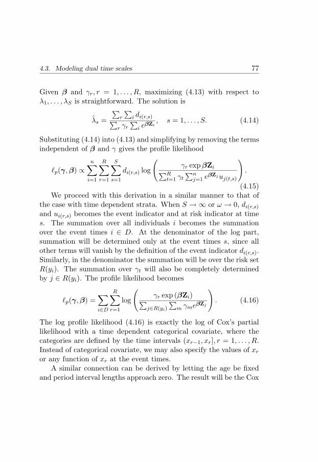
4.3. Modeling dual time scales 77
Given β and γr, r = 1, . . . , R, maximizing (4.13) with respect toλ1, . . . , λS is straightforward. The solution is
λs =
∑r
∑i di(r,s)∑
r γr∑
i eβZi, s = 1, . . . , S. (4.14)
Substituting (4.14) into (4.13) and simplifying by removing the termsindependent of β and γ gives the profile likelihood
ℓp(γ, β) ∝
n∑
i=1
R∑
r=1
S∑
s=1
di(r,s) log
(γr expβZi∑R
t=1 γt∑n
j=1 eβZjuj(t,s)
).
(4.15)We proceed with this derivation in a similar manner to that of
the case with time dependent strata. When S → ∞ or ω → 0, di(r,s)
and ui(r,s) becomes the event indicator and at risk indicator at times. The summation over all individuals i becomes the summationover the event times i ∈ D. At the denominator of the log part,summation will be determined only at the event times s, since allother terms will vanish by the definition of the event indicator di(r,s).Similarly, in the denominator the summation will be over the risk setR(yi). The summation over γt will also be completely determinedby j ∈ R(yi). The profile likelihood becomes
ℓp(γ, β) =∑
i∈D
R∑
r=1
log
(γr exp (βZi)∑
j∈R(yi)
∑m γmeβZj
). (4.16)
The log profile likelihood (4.16) is exactly the log of Cox’s partiallikelihood with a time dependent categorical covariate, where thecategories are defined by the time intervals (xr−1, xr], r = 1, . . . , R.Instead of categorical covariate, we may also specify the values of xr
or any function of xr at the event times.A similar connection can be derived by letting the age be fixed
and period interval lengths approach zero. The result will be the Cox

78 4.4. Simulation studies
proportional hazards model with (age) entering as time dependentstrata or as a time dependent covariate in the model with basic timescale calendar time.
Other pairs of time scales are of course possible. For instance,dual time scales age and time since diagnosis arise frequently inclinical studies, age and time since weaning is another example fromchildhood life studies.
4.4 Simulation studies
4.4.1 Erroneous scale
The first simulation study investigates the performance of proce-dures to select relevant time scales discussed in Section 4.2. Theprocedures are the proportional hazards assumption test and frailtymodel estimation.
Several data generating models are assumed. We consider twocompeting time scales S1 with duration T1 and S2 with duration T2.S1 was specified as a better time scale than S2 in the sense that S1
has lower value of time delay δi than S2 has. One example in a realstudy, the true time scale is time since the onset of certain disease,T1 is time since the subject feels any symptoms of the disease andT2 is time since diagnosis. We assume that the time since onset cannot be determined by the diagnosis.
The true duration T is generated by the ordinary proportionalhazards model,
λi(t) = λ0(t) exp(βZi), t > 0, (4.17)
but we can only observe T1 and T2 generated from the true timescale with delays δi for each individual i. The details of the simula-tion procedure is described in the Appendix A-1. No truncation or

4.4. Simulation studies 79
censoring is considered in this simulation. Similar simulation stud-ies have been considered by Liestøl and Andersen (2002) for theGompertz-Makeham baseline hazard function with the purpose ofshowing the effect of misalignment patients and measurement erroron the estimated regression coefficients.
To make S1 better than S2, the mean of δi for T1 was speci-fied lower than that for T2 and δi follows uniform and exponentialdistributions. For this simulation the baseline hazards were deter-mined parametrically as Gompertz, Exponential or Weibull hazardfunctions. One fixed categorical zero-one covariate Zi generated thefrom Bernoulli distribution was also included.
Now, we compare the performance of the proportional hazardtest (ph-test) and frailty variance estimation to detect the relevanttime scales. The relevant time scale is expected to satisfy the propor-tional hazards assumption, and therefore will have larger p-values.In the frailty model, the estimated gamma frailty variance is used todetect the relevant time scale. A smaller frailty variance will indi-cate a better time scale. In a real situation, a more careful analysiscan be performed. For example, a Schoenfeld residuals plot may beused to accompany the ph-test, and a confidence interval constructedfrom the profile likelihood may be calculated for the gamma frailtyvariance.
In the simulation the mean and standard deviation of the ph-testp-value and gamma frailty variance are used to summarize the resultfrom 1000 replications. Histograms of the values are also examined(results not shown). In Tables 4.1 and 4.2 the mean of the ph-testp-value is under the zph column, and the mean of the gamma frailtyvariance is in the ω column.
There are some general comments for the generated data. Thedelays (δi) that follows an exponential distribution seems to makethe model suffering from the violation of the proportional hazardsassumption, shown by the low value of the coverage (the percentage

80 4.4. Simulation studiesTab
le4.1:
Sim
ulation
study
forerron
eous
scalew
ithδifollow
suniform
distrib
ution
U(0,1)
and
U(0.5,2),
forS
1an
dS
2resp
ectively.
The
true
coeffi
cientβ
is2.
Each
value
iscalcu
latedbased
ona
sample
ofsize
200w
ith1000
replication
sTim
eSca
leB
aselin
eM
odel
S1
S2
haza
rds
βp
zph
ωβ
pzph
ω
Gom
pertz
CP
H1.9
894.8
0.6
5–
1.9
291.8
0.6
3–
0.1
9–
0.2
5–
0.1
9–
0.2
5–
CP
HF
1.9
994.2
0.6
60.0
09
1.9
994.2
0.6
60.0
09
0.2
1–
0.2
30.0
39
0.2
1–
0.2
30.0
39
Exponen
tial
CP
H1.6
447.8
0.4
4–
1.4
39.6
0.4
1–
0.1
8–
0.2
7–
0.1
6–
0.2
8–
CP
HF
1.6
448.2
0.4
40.0
01
1.4
39.6
0.4
10
0.1
8–
0.2
70.0
10.1
6–
0.2
80.0
01
Weib
ull
CP
H1.8
585.8
0.5
8–
1.7
059.6
0.5
3–
0.1
9–
0.2
6–
0.1
9–
0.2
7–
CP
HF
1.8
585.8
0.5
90.0
04
1.7
060.0
0.5
40.0
02
0.1
9–
0.2
60.0
28
0.1
9–
0.2
70.0
16
pis
the
covera
ge
(percen
tage)
ofth
ein
tervalestim
atio
nC
oxP
H:C
ox’s
pro
portio
nalhaza
rds
βis
the
mea
nofestim
ated
coeffi
cient
CoxP
HF
:C
ox’s
pro
portio
nal
zph
isth
em
ean
ofpro
portio
nalhaza
rds
testp-v
alu
ew
ithfra
ilty
ωis
the
mea
nofestim
ated
frailty
varia
nce
The
valu
esin
every
second
row
are
standard
dev
iatio
ns

4.4. Simulation studies 81Tab
le4.
2:Sim
ula
tion
study
forer
roneo
ussc
ale
wit
hδ i
follow
sex
pon
enti
aldis
trib
uti
onw
ith
mea
n0.
5an
d1.
25,
forS
1an
dS
2re
spec
tivel
y.T
he
true
coeffi
cien
tβ
is2.
Eac
hva
lue
isca
lcula
ted
bas
edon
asa
mple
ofsi
ze20
0w
ith
1000
replica
tion
s
Tim
eSca
leB
ase
line
Model
S1
S2
haza
rds
βp
zph
ωβ
pzph
ω
Gom
per
tzC
PH
1.8
787.0
0.6
3–
1.4
413.6
0.3
4–
0.2
0–
0.2
5–
0.2
0–
0.3
0–
CP
HF
1.9
087.0
0.6
60.0
21.6
548.8
0.5
70.1
69
0.2
2–
0.2
20.0
67
0.2
8–
0.1
90.1
9E
xponen
tial
CP
H1.2
31.2
0.3
6–
0.7
00.0
0.1
3–
0.1
9–
0.2
9–
0.1
8–
0.2
1–
CP
HF
1.3
919.6
0.5
00.1
47
1.0
410.0
0.2
50.4
25
0.2
6–
0.2
10.1
96
0.3
6–
0.1
80.4
17
Wei
bull
CP
H1.5
528.2
0.5
1–
0.9
40.0
0.1
3–
0.1
8–
0.2
9–
0.1
8–
0.2
0–
CP
HF
1.6
346.2
0.6
10.0
69
1.3
122.6
0.3
40.3
75
0.2
3–
0.2
00.1
24
0.3
2–
0.1
60.3
04
pis
the
cover
age
(per
centa
ge)
ofth
ein
terv
ales
tim
ation
CoxP
H:C
ox’s
pro
port
ionalhaza
rds
βis
the
mea
nofes
tim
ate
dco
effici
ent
CoxP
HF
:C
ox’s
pro
port
ional
zph
isth
em
ean
ofpro
port
ionalhaza
rds
test
p-v
alu
ew
ith
frailty
ωis
the
mea
nofes
tim
ate
dfr
ailty
vari
ance
The
valu
esin
ever
yse
cond
row
are
standard
dev
iations
82 4.4. Simulation studies
of confidence intervals covering the true coefficient β). The mostsuffering one is the model with exponential baseline hazard.
When the baseline hazard function follows a Gompertz model,both the ph-test and frailty model show good performances. In Table4.1, S1 and S2 are equally good, whereas in Table 4.2, S1 is betterthan S2 showed by the larger value of zph and smaller ω. Theperformances are confirmed by the coverage percentages p whichhave lower value for the wrong time scale.
Exponential baseline hazards are very much affected by the er-roneous scale. Although the zph’s do not show very low values andω’s do not show very large values, the coverage probabilities are verylow. In Table 4.1, it is rather hard to distinguish the time scales,because the values of zph and ω look similar, but the coverage prob-abilities are quite low for S2. For a larger effect of erroneous scale inTable 4.2, S1 and S2 can be distinguished by the value of zph and ω.The estimated frailty variances in the exponential baseline hazards(Table 4.1) do not seem to reveal the frailty effect. They give smallvariances but actually the effect is rather bad (lower coverages).
The performance of the procedures under the Weibull baselinehazard is generally similar with that of Gompertz. In the Weibullhazard the delays has a larger effect than in the Gompertz. The zphand ω can distinguish S1 and S2 in the data with a larger effect oferroneous scale.
When the procedures do not show a difference between S1 and S2,dual time scales modeling may be performed. For the data generatedfrom these erroneous scale models, the inclusion of other time scalesin the analysis will not likely increase the model fit.
4.4.2 Dual time scales
The second simulation study considered the approach discussed inSection 4.3 for modeling dual time scales S1 and S2. In a real study,

4.4. Simulation studies 83
S1 and S2 could be calendar time and age, or age and time since di-agnosis. In this simulation we assume the true model that generatesduration T1 as a result of using S1 follows a Cox model with timedependent covariate
λi(t | Z(t)) = θ exp(β1ηi + β2(t + δi)), t > 0. (4.18)
For example, T1 is time since onset of certain disease, T2 is the ageand δi is the age at onset, so where T1 = T2 − δ. For positive β2
the hazard for individual i will increase with time and the hazardis higher for individuals with higher δi (higher age at onset). Thedetails of the data generating procedure of this simulation are pre-sented in Appendix A-2.
In reality, we do not know the exact data generating process, weonly believe that T1 and T2 should be modeled simultaneously. Thecompared performances for this simulation are the estimation of β1
(the mean estimation, standard deviation) and the mean of the ph-test p-value (for analysis with Cox’s model). One example of dualanalysis is in the childhood mortality studies (Section 3.2). We maybelieve that the mortality depends on age and seasonality, thereforeboth time scales, age and period (as the proxy of seasonality), haveto be taken care of. The variables of interest are not the timesthemselves but other explanatory variables such as gender, maternaleducation, etc. How the method of taking care of T1 and T2 affectsthe explanatory variable of interest is what we want to compare.
For the piecewise constant hazard approach, each time scale weredivided into four equal-width intervals. Experimenting with severalvariations of gridding for generated data used in this simulation,four intervals gave reasonable piecewise constant hazards and wascomputationally feasible.
For the time-dependent strata, the same intervals as in the piece-wise constant hazards were used. The analysis used the count-ing process data setup (Section 2.2). For each generated data set,

84 4.4. Simulation studies
Table 4.3: Simulation study for dual time scales S1 and S2 analyzedwith piecewise constant hazards and time dependent approaches.The true coefficients are β1 = 1.5, β2 = 0, 1 and δi is exponentialwith rate 0.85. Each value is calculated based on a sample of size200 with 1000 replications
Method β2 = 0 β2 = 1β1 (sd) p1 zph β1 (sd) p1 zph
piecewise const-hzd 1.55(.18) 95.2 – 1.51(.15) 95.5 –S1 time-dep strata 1.51(.19) 94.9 .81 1.50(.18) 95.7 .71S2 time-dep strata 1.51(.19) 95.2 .63 1.51(.18) 96.4 .66S1 time-dep covariate 1.51(.18) 95.3 .90 1.48(.16) 95.7 .98S2 time-dep covariate 0.91(.13) 5.6 .89 0.58(.13) 0.1 .99
S1 and S2 in front of the method’s name denotes the basic time scale used
two time-dependent strata estimation procedures were carried out.The first one used S1 as the basic time scale with S2 as the time-dependent stratum, and the second used S2 as the basic time scalewith S1 as the time-dependent stratum.
In the Cox time-dependent covariate analysis, the values of thecovariate are only used at event times with a certain functional form.Analyzing time-dependent covariates in that way is computationallydemanding, therefore we used similar time intervals as in the piece-wise constant hazard and the time-dependent strata method. Theform of the function is modeled non-parametrically using penalizedsmoothing spline (Hastie and Tibshirani, 1990), which is available,for instance, in the survival package of R or S-PLUS. As in the time-dependent strata case, two analyses were carried out by this modelusing each time scale and including the other time scale as a time-dependent covariate.
The results are shown in Table 4.3 for exponentially distributedδi and in Table 4.4 for uniformly distributed δi.

4.4. Simulation studies 85
Table 4.4: Simulation study for dual time scales S1 and S2 analyzedwith piecewise constant hazards and time dependent approaches.The true coefficients are β1 = 1.5, β2 = 0, 1 and δi is uniform(0,2).Each value is calculated based on a sample of size 200 with 1000replications
Method β2 = 0 β2 = 1β1 (sd) p1 zph β1 (sd) p1 zph
piecewise const-hzd 1.53(.17) 95.1 – 1.50(.15) 96.4 –S1 time-dep strata 1.51(.18) 95.4 .81 1.49(.18) 95.7 .74S2 time-dep strata 1.51(.18) 94.8 .61 1.50(.15) 97.6 .47S1 time-dep covariate 1.50(.18) 95.1 .97 1.48(.17) 95.2 .95S2 time-dep covariate 0.88(.13) 3.1 .92 0.50(.11) 0.0 .93
S1 and S2 in front of the method’s name denotes the basic time scale used
In general, piecewise constant hazard and time-dependent stratashow good performances. For the time-dependent strata, the appro-priate analysis assuming model 4.18 is to use S1 as the basic timescale which gave good performances. However, even if the inappro-priate basic time scale S2 is used, the performances are also goodwith only slightly violated proportional hazards assumption.
For the time-dependent covariate approaches, using S1 as the ba-sic time scale gave good performances which is not surprising giventhe data generating model. Using the wrong basic time scale S2 isreally harmful and worse if the time-dependent covariate is reallyin the model, i.e., β2 = 1. Simulation with β2 = 0 complementsthe result given by Liestøl and Andersen (2002). In their simulationT1 is ’time since diagnosis’ which had a Gompertz form and T2 isage. The Gompertz baseline hazard is convenient since T1 can switchinto time-dependent covariate and still give the same result. In thissimulation it is shown that a baseline hazard other than the Gom-pertz (constant hazard in this simulation) will give different results.

86 4.5. Application to infant mortality age-period analysis
This issue has also been discussed for the case of an epidemiologicalfollow-up study by Korn, Graubard and Midthune (1997).
4.4.3 Miss-specification
We also analyzed the generated data sets under miss-specified analy-sis, i.e., (i) the data was generated from the erroneous scale modelbut analyzed with the dual time scales methods; (ii) the data wasgenerated from the dual time scales model but analyzed with theerroneous scale methods.
For the first miss-specified analysis, all dual time scales ap-proaches showed good performances for the low effect of erroneousscale (the Gompertz baseline hazard case) but not for the large effectof erroneous scale (the exponential baseline hazard case). The Coxmodels with time-dependent strata and piecewise constant hazardsapproaches have similar performances and they are better than theCox model with a time-dependent covariate.
For the second miss-specified analysis, the exponentially distrib-uted δi, the ph-test and frailty model suggest that S1 is the mostrelevant time scale. However, for the uniformly distributed δi theprocedures do not show any difference.
4.5 Application to infant mortality
age–period analysis
We look again at the application considered in Section 3.2 aboutinfant and child mortality. We mainly concentrate on the dual timescales age-period problem with categorical covariates gender (boy orgirl) and maternal education (none, 6, 9, 12 years of education) forinfant mortality data.

4.5. Application to infant mortality age-period analysis 87
Analyses with piecewise constant hazards, Cox’s proportionalhazards with age time scale and Cox’s proportional hazards with pe-riod time scale were performed. Two-month grids were applied forboth age and period. For the piecewise constant hazards model, thestandard Poisson model for the number of events in each grid withlog link function was used. The total exposure times in each grid wasentered to the model as an offset. For the Cox model with age timescale, period time was included as time-dependent strata or time-dependent covariate. Similarly, in the Cox model with period timescale, age was included as time-dependent strata or time-dependentcovariate. The time-dependent covariates in both models using ageand period as the basic time scale were treated non-parametricallyusing a penalized smoothing spline.
There is no scientific background suggesting that the two timescales, age and calendar time, are two alternative time scales. How-ever, we can examine this by checking the proportionality assump-tion of the model using age and period as the basic time scale inseparate analyses. No model violates the proportionality assumptionwith relatively large p-values for the proportionality test of 0.332 and0.763 for age and period time scale, respectively.
Tables 4.5 and 4.6 show the result of likelihood ratio tests for thevariables in each model and estimated coefficients, respectively. Inthis particular data set, in fact, they gave similar results. However,the safe approach is to consider the results from a Cox model with thetime-dependent strata or piecewise constant hazards method. Thegeneral conclusion is that maternal education is quite important andgives protective effect in the case of infant mortality.

88 4.5. Application to infant mortality age-period analysis
Table 4.5: Likelihood ratio test (LRT) for variables in the infant mor-tality models using piecewise constant hazards (pc-hazards), Coxproportional hazards with age time scale (Cox-age), Cox propor-tional hazards with period time scale (Cox-period)
Variables pc-hazards Cox-age Cox-periodtd-strata td-covar td-strata td-covar
Age < .001 — — — < .001Period .395 — .979 — —Gender .080 .100 .075 .104 .132Maternal educ. < .001 < .001 < .001 < .001 < .001
Table 4.6: Estimated coefficients and their standard errors for genderand maternal education in the infant mortality models
Variables pc-hazards Cox-age Cox-periodtd-strata td-covar td-strata td-covar
Genderboy — — — — —girl -0.31 (.18) -0.29 (.18) -0.32 (.18) -0.29 (0.18) -0.29 (.19)
Maternal educ.none — — — — —6 years -0.76 (.26) -0.76 (.27) -0.74 (.26) -0.72 (.27) -0.53 (.28)9 years -1.17 (.34) -1.18 (.35) -1.16 (.34) -1.11 (.35) -1.10 (.36)12 years -2.74 (.56) -2.72 (.56) -2.70 (.56) -2.67 (.56) -2.43 (.57)

4.6. Remarks 89
4.6 Remarks
The first consideration when we face a multiple time scales problemin event history analysis is to look for the scientific background ofthe time scales. The background may be obvious in clinical studiesbut may not be so in epidemiological or observational studies.
A proportional hazards test is advisable for checking the alterna-tive time scales. This procedure is simpler than using a frailty model,moreover analyzing individual frailty may give wrong conclusions, es-pecially when we use an incorrect underlying frailty distribution. Wehave noticed this problem also in the simulation studies.
A safe approach in analyzing dual time scales is to use the Coxmodel with time-dependent strata or the piecewise constant hazardapproach. Simulation studies showed that both approaches gavegood performance when analyzing dual time scales generated by theerroneous scale model or by the dual time scales model. The Coxmodel with time-dependent covariate is superior to other approacheswhen the other time scale (than the basic time scale) is really a time-dependent covariate in the model.

90 4.6. Remarks

Chapter 5
Event History Analysis
with Longitudinal
Measurements
5.1 Introduction
We consider modeling event history with longitudinal measurementswhen the longitudinal measurements are intermittently observed andeventually measured with errors. Analysis of respiratory infectionand weight in the ZINAK study presented in Chapter 3 is one ex-ample of such a situation.
One way of analyzing such data is by considering the time-to-event data as the outcome and longitudinal measurements as a time-dependent covariate. Another way is to analyze both outcomes si-multaneously assuming that they are independent given certain la-tent processes.
Several methods have been proposed to deal with this kind ofproblem and some of them have been reviewed in Section 2.4.1. Four
91

92 5.2. Problem and models
methods that have been around in the literature are LVCF (LastValue Carried Forward), TEL (time elapsed since the last measure-ment), two-stage, and joint model of event time and longitudinalmeasurements. Two methods based on Cox’s proportional hazardsmodel with stratification and frailty are proposed. The emphasisof the analysis is on the joint evolution of time-to-event and lon-gitudinal measurements rather than longitudinal measurements assurrogate markers for the event.
To our knowledge, all methods mentioned above were mostly ap-plied to clinical settings such as AIDS studies, psychiatric disordersand cancer prevention trials, not to observational or epidemiologicalsettings which are more ”irregular” than the clinical ones. Applica-tions of the methods to multiple events or repeated events are alsorarely considered in the literature.
The aim of this chapter is to compare the methods by means ofsimulation and to perform further analysis of the respiratory infec-tion and weight data from the ZINAK study introduced in Chapter 3.
5.2 Problem and models
Suppose n individuals are followed over a time interval [0, L) withlongitudinal measurements yij : i = 1, 2, . . . , n; j = 1, 2, . . . , niat times tij : i = 1, 2, . . . , n; j = 1, 2, . . . , ni. Together with themeasurements, a counting process Ni(u) : 0 ≤ u ≤ L for theevents and a predictable at risk process Ki(u) : 0 ≤ u ≤ L are alsorecorded. An additional fixed time covariate or baseline covariate Z
may be included.One example of such a data setup is illustrated in Figure 5.1. The
event history data are repeated events data in which one individualmay have several counting process intervals (t0, t1], event. Theat-risk process Ki(u) : 0 ≤ u ≤ L is alternating between 0 and 1
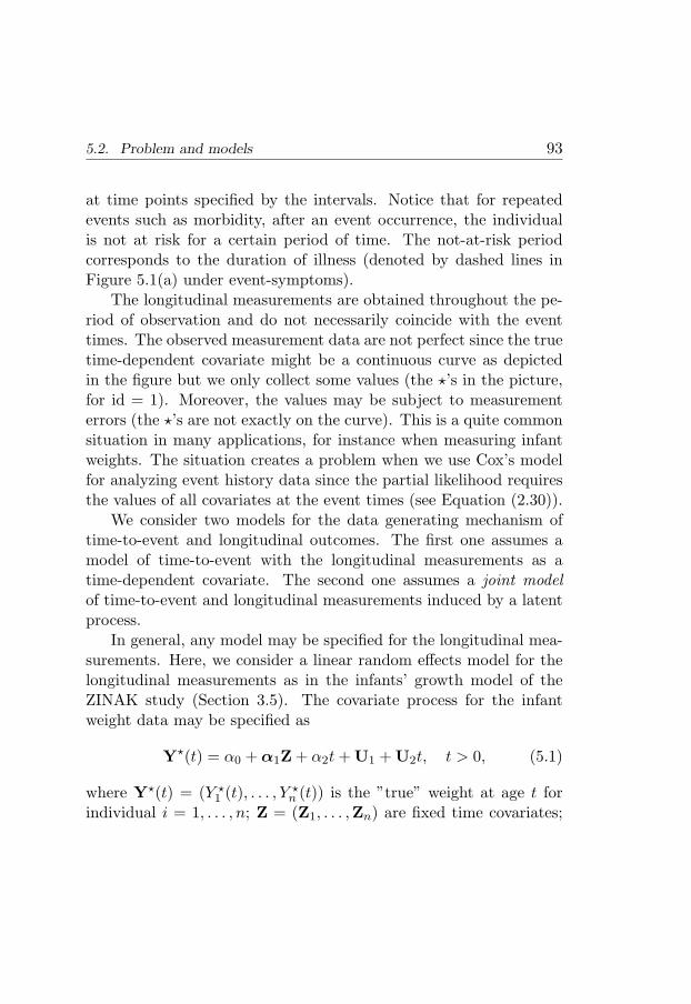
5.2. Problem and models 93
at time points specified by the intervals. Notice that for repeatedevents such as morbidity, after an event occurrence, the individualis not at risk for a certain period of time. The not-at-risk periodcorresponds to the duration of illness (denoted by dashed lines inFigure 5.1(a) under event-symptoms).
The longitudinal measurements are obtained throughout the pe-riod of observation and do not necessarily coincide with the eventtimes. The observed measurement data are not perfect since the truetime-dependent covariate might be a continuous curve as depictedin the figure but we only collect some values (the ⋆’s in the picture,for id = 1). Moreover, the values may be subject to measurementerrors (the ⋆’s are not exactly on the curve). This is a quite commonsituation in many applications, for instance when measuring infantweights. The situation creates a problem when we use Cox’s modelfor analyzing event history data since the partial likelihood requiresthe values of all covariates at the event times (see Equation (2.30)).
We consider two models for the data generating mechanism oftime-to-event and longitudinal outcomes. The first one assumes amodel of time-to-event with the longitudinal measurements as atime-dependent covariate. The second one assumes a joint modelof time-to-event and longitudinal measurements induced by a latentprocess.
In general, any model may be specified for the longitudinal mea-surements. Here, we consider a linear random effects model for thelongitudinal measurements as in the infants’ growth model of theZINAK study (Section 3.5). The covariate process for the infantweight data may be specified as
Y⋆(t) = α0 + α1Z + α2t + U1 + U2t, t > 0, (5.1)
where Y⋆(t) = (Y ⋆1 (t), . . . , Y ⋆
n (t)) is the ”true” weight at age t forindividual i = 1, . . . , n; Z = (Z1, . . . ,Zn) are fixed time covariates;

94 5.2. Problem and models
(a) event - symptoms
id=1
id=2
id=3
longitudinal measurements
id=1⋆
⋆
⋆
⋆
2
3
4
0 2 4 6 8 10
time t
(b)id t0 t1 event
1 0 6 11 7 10 02 0 3 12 4 9 13 0 5 13 7 10 0
(c)id t Y
1 2 2.91 4 4.21 6 51 8 4
Figure 5.1: (a) Event history data and longitudinal measurementsand an illustration of imputing time-dependent covariate values us-ing LVCF and time since measurements; (b) event history data (c)longitudinal data

5.2. Problem and models 95
U1 and U2 are the unobservable random effects for the intercept andage t with (U1,U2) ∼ N(0,Σ). The observed covariate process is
Y(t) = Y⋆(t) + ǫt, t = t1, t2, . . . , (5.2)
where ǫt ∼ N(0, σ) are the measurements errors. The actual ob-servation Y(t) is not continuously observed but finitely observed attimes t1, t2, . . ..
The time-to-event is modeled through Cox’s proportional hazardsmodel
λ(t | X, Y ⋆(t)) = λ0(t) exp(β1X + β2Y⋆(t)), (5.3)
where X are fixed time covariates such as maternal education, sup-plementation and may also include Z (e.g., the gender variable inthe covariate process model).
The central methodological and practical problem is how to es-timate the parameters in (5.3) when Y ⋆(t) is not available but Y (t)is instead. The methods we consider are LVCF, TEL, two-stage,Cox-frailty and Cox-strata discussed in the next section.
The joint model was mentioned in Section 2.4.2 as a more generalmethodology to deal with time-dependent covariates. It has two sub-models, one for the longitudinal measurements and another for thetime-to-event.
The longitudinal measurements model is the same as model (5.2).The specification of the time-to-event model, however, is differentfrom that of (5.3). The hazard function of this joint model is
λ(t | X) = λ0(t) exp(βX + γ(U1 + U2t)), (5.4)
where X are fixed time covariates, could be the same or overlapwith Z; U1 and U2 are specified similarly as in model (5.3). Thedifference compared to model (5.3) is that the ”true” value Y ⋆(t) arenot included in the hazard function but only the random effect partU1 + U2t.

96 5.3. Methods
The idea of the joint model is that the dependence between thelongitudinal measurements and the time-to-event can arise throughthe common covariate X and the possible unobserved heterogeneityin both models. The joint model attempts to take care of the la-tent heterogeneity in both models simultaneously. When there is nolatent association, γ = 0, the joint model is actually two separatemodels of longitudinal data and event history data.
It is also possible to include more random effect terms thanU1 + U2t. The latent association can also be extended as in theHenderson et al.’s (2000) model and there can even be more thanone longitudinal measurement (Lin, McCulloch and Mayne, 2002).However, in many practical situations, the random effects term ofthe initial value of measurement (the intercept) and the steepness ofthe longitudinal covariate by time (e.g., age) are the most importantterms.
5.3 Methods
The four methods of LVCF, TEL, two-stage and joint model havebeen reviewed briefly in Section 2.4.2. We discuss the methods fur-ther here with some illustrations.
Suppose we have event history data and longitudinal data as inFigure 5.1. To construct LVCF and TEL for the individual withid = 1, we have to know the covariate value for this individual atthe event times 3, 5, 6, and 9.
The values obtained by the LVCF method are the symbol inFigure 5.1. They are obtained by assuming that the most recentmeasurement value is the value at event-time. It is possible thatthe event-times correspond to the covariate-time (as at t = 6, thesymbol ⋆ ). The time elapsed since the last measurement (TEL) is

5.3. Methods 97
the length of the horizontal line connecting the actual measurementand the event time.
The LVCF and TEL methods are used in the ordinary Cox re-gression as
λ(t | Z, Yt) = λ0(t) exp(βZ + Yt), (5.5)
λ(t | Z, Yt, τ) = λ0(t) exp(βZ + Ytf1(τt) + f2(τt)), (5.6)
respectively, where Z are fixed-time covariates; Yt denotes the valueobtained by LVCF, τt is the TEL at t, f1 and f2 are suitable func-tions.
The LVCF method is known to give biased estimates of the pa-rameters (Prentice, 1982). However, we believe that LVCF is com-monly used in practice. The Yt could be a good predictor of hazardwhen the effect of the longitudinal measurements on event time isdelayed.
The idea of the TEL method is that the measurements could be”aging” and new information closer to the event time is better thanold information. When the measurements are irregularly observed,the value of τt (TEL) could carry information about the subjectsdisease progression (Bruijne et al., 2001). However, it is not likelyto be an added advantage for regular measurements such as in theZINAK study. The added difficulty in using TEL instead of LVCF isin specifying f1 and f2. Therefore, the skill and tool needed in TELis actually the same as modeling the ordinary Cox regression. Thismethod could be a practical alternative to more complex sophisti-cated methods.
The two-stage method is mentioned briefly in Section 2.4.2. Themain idea of the method is to reconstruct the covariate function giventhe observed values of the covariate. In the two-stage approach,Cox’s proportional hazards model becomes
λ(t | Z, Yt) = λ0(t) exp(β1Z)E [exp(β2Y⋆(t)) | K(t) = 1, Yt,Z] ,
(5.7)

98 5.3. Methods
where Z are fixed-time covariates always available at the event times;Yt denotes the observed values (the Y(t) in model (5.2)); and K(t) =IT≥t is an at-risk process indicator function (the usual notationY (t) for the at-risk process has been reserved for the longitudinalmeasurements). Tsiatis et al. (1995) used a first-order approximationof the conditional expectation in model (5.7).
The LVCF, TEL and two-stage methods basically assume thefirst model discussed in Section 5.2 (Equations (5.1), (5.2), and(5.3)) where the central problem is on imputing missing longitu-dinal covariate values at the event times. The two-stage model ismore computationally demanding than the others since it needs tofit a longitudinal model at each event time.
The joint model method assumes the joint model of the time-to-event and longitudinal measurements process induced by a latentprocess discussed in Section 5.2. We have mentioned several meth-ods to fit the model in Section 2.4.2. Basically, the joint methodmaximizes the likelihood function of longitudinal and hazard modelsimultaneously. Theoretically, it has many desirable properties,such as less biased parameter estimates, making the efficient useof data and easier model validation (Tsiatis et al., 1995; Hendersonet al., 2000; Ibrahim, Chen and Sinha, 2001; Tsiatis and David-ian, 2004). Practically, the methods developed for this model arestill lacking computational tools and this model is computationallydemanding (Do, 2002).
In addition to the methods discussed above, we propose twomethods based on Cox’s model with stratification and Cox’s modelwith frailty. We call them Cox-strata and Cox-frailty, henceforth.The main idea of both methods is adjustment for the longitudinalcovariate when the covariate is considered as a nuisance variable. Forexample, when the interest is not on the effect of weight on the mor-bidity but on the effect of other variables such as supplementation,

5.3. Methods 99
gender or maternal education, these methods could be a reasonablechoice.
Basically we assume a constant multiplicative effect of exp(Y ⋆(t))on the baseline hazard function over time. This assumption may beviolated when we use Y (t) as a proxy of Y ⋆(t). Stratification is theusual approach to deal with non-proportionality.
In this longitudinal measurements problem, the Y (t) is time de-pendent, therefore the stratification is actually a time-dependentstratification. Cox’s model with time-dependent strata is
λ(t | Z, Y (t)) = λ0yj (t) exp(βZ), if Y (t) = yj , (5.8)
where yj is the value of Y (t), j = 1, 2, . . . , V , where V is the numberof unique values of Y (t).
In practice, when V is large, the Cox-strata method may not befeasible and the precision of estimated coefficients may be low. Toovercome this, we may categorize Y (t) such that the size of V isreasonable.
The term exp(β2Y⋆(t)) in model (5.3) which is a random variable
instead of a fixed variable also leads naturally to Cox’s model withfrailty (Section 2.2.5, Equation (2.13)). In this case, clusters in thisfrailty model are the longitudinal measurements, therefore we use thevalue of the longitudinal measurements as a categorical variable, thesame as yj in the Cox-strata method. In fact, this frailty approachis one alternative solution when the V in the Cox-strata method islarge.
Practically, we may use the value obtained by the LVCF methodor by the two-stage method for the value of Y (t). The problem ofspecifying the distribution of the frailty effects is the same as inany Cox’s frailty model. We have discussed this problem for thechildhood mortality model (Chapter 3) and the multiple time scalesproblem (Chapter 4).

100 5.4. Simulation studies
5.4 Simulation studies
The purpose of the simulation study is to investigate the performanceof the methods discussed in the previous section. We compared theLVCF, TEL, two-stage, Cox-frailty and Cox-strata methods. Thejoint model was not included in the comparison since, as we havenoticed in the previous section, it requires heavy computation andis not feasible for large simulations.
The simulated data for each individual consists of event historydata (t0, t1], event with one fixed covariate Z and longitudinal data(t, Yt), similar to the illustration in Figure 5.1. The fixed covariatecould be supplementation, gender or maternal education as in theZINAK study. The details of the simulation procedures are found inAppendix A-3. Simulations were performed in R (Ihaka and Gen-tleman, 1996; R Development Core Team, 2004).
We look at β1, the estimated coefficient of Z, as one criterionof method performances. The coverage, an indicator whether theinterval estimation includes the true parameter or not, were calcu-lated. Proportionality of the hazard model is another criterion tobe investigated. Additionally we also looked at β2, the estimatedcoefficients of the longitudinal measurements Y , for the LVCF, TELand two-stage methods.
Tables 5.1 and 5.2 show the results of the simulations based onthe two main models discussed in Section 5.2. When there is nocovariate effect in the hazard model (5.3) or no latent association inmodel (5.4), that is β2 = 0, all methods arrived at similar results.The performance of the methods in estimating β1 were similarly goodwith coverages close to 95%. The performance investigated from theproportionality assumption was also good for all methods but theTEL method generally has better hazard proportionality than theothers.
For the LVCF, TEL and two-stage methods, we can also look at

5.4. Simulation studies 101
Table 5.1: Simulation study for Cox’s time-dependent covariatemodel analyzed with the LVCF, TEL, two-stage, Cox-frailty andCox-strata methods. See the text and Appendix A-3 for the simu-lation specifications. Each value is calculated based on a sample ofsize 50 with 500 replications
Method β2 = 0 β2 = −0.1β1 (sd) p1 zph β1 (sd) p1 zph
LVCF 1.23 (.170) 94.3 .477 1.24 (.232) 95.2 .498TEL 1.23 (.170) 94.1 .547 1.24 (.233) 95.2 .580Two-stage 1.22 (.167) 95.5 .507 1.24 (.236) 95.3 .505Cox-strata 1.23 (.271) 94.7 .510 1.24 (.361) 95.0 .492Cox-frailty 1.23 (.168) 95.3 .492 1.24 (.232) 95.6 .490
β1 is the mean of the estimated coefficient β1 (true value β1 = 1.2) and
their standard deviation (sd) in parentheses
p is the coverage (percentage) of the interval estimation
zph is the mean of the proportional hazards test p-value
Table 5.2: Simulation study for joint model analyzed with the LVCF,TEL, two-stage, Cox-frailty and Cox-strata methods. See the textand Appendix A-3 for the simulation specifications. Each value iscalculated based on a sample of size 50 with 500 replications
Method β2 = 0 β2 = 1β1 (sd) p1 zph β1 (sd) p1 zph
LVCF 1.20 (.193) 94.8 .512 1.01 (.254) 78.4 .429TEL 1.20 (.196) 94.6 .589 1.01 (.257) 78.4 .510Two-stage 1.22 (.203) 94.5 .493 1.02 (.259) 78.6 .441Cox-strata 1.22 (.365) 96.0 .515 1.03 (.447) 85.1 .478Cox-frailty 1.20 (.160) 95.5 .508 1.04 (.207) 84.5 .476
β1 is the mean of the estimated coefficient β1 (true value β1 = 1.2) and
their standard deviation (sd) in parentheses
p is the coverage (percentage) of the interval estimation
zph is the mean of the proportional hazards test p-value

102 5.4. Simulation studies
the performance based on the estimates of β2. The β2 were almostperfectly estimated with mean of 0.003, 0.002, and 0.002; coverage94.9%, 95.7% and 94.1%, for the LVCF, TEL and two-stage methods,respectively.
When data was generated by Cox’s time-dependent covariatemodel and the effect of covariate Y was present, i.e., β2 = −0.1(Table 5.1), the performance of all methods were as good as that ofthe result with β2 = 0. It is rather surprising that the LVCF methodis similarly good enough to estimate β1 for this situation as comparedto the two-stage method, except perhaps for its proportionality. TheLVCF method is probably good when the time-dependent covariateis a linear model with low gradient, as specified for Y in this simu-lation.
For the LVCF, TEL and two-stage methods, their estimates ofβ2 were rather poor with means of -0.005, -0.013, and -0.005, respec-tively; coverage 82.2%, 89.8% and 83%, respectively. This problemwas due to the measurement errors of Y . The estimation of β2 wasslightly better with the TEL method.
When data were generated from the joint model with latent asso-ciation (Table 5.2), the estimates of β1 were biased for all methods.Here, the Cox-strata and Cox-frailty methods are slightly better thanthe LVCF, TEL and two-stage methods with larger coverage proba-bility. The performances dramatically went down for the LVCF, TELand two-stage methods in estimating β2. Their estimates were closeto zero and far from the true value 1 of β2. Their coverage were closeto zero as well. These severe under-estimations were largely causedby the miss-specification of Y .

5.5. Application to infant respiratory infection and weight data 103
5.5 Application to infant respiratory infec-
tion and weight data
We continue the analysis of infants respiratory infection and weightdata from the ZINAK study introduced in Chapter 3. We includedthe weight longitudinal covariate in the hazard model and analyzedthe data using the LVCF, TEL, two-stage, Cox-strata and Cox-frailty, and joint model methods.
We used both the Andersen-Gill model (AG model) and the gap-time model to specify the model of repeated events. We expectimprovements over the models presented in Table 3.7 (the AG model)and Table 3.8 (the gap-time model) by using these methods.
The implementation of the LVCF method to the data is straight-forward but rather tedious. First we have to arrange the data byevent-time splitting (See example in Figure 5.1, Section 5.2). Therewere 2,423 records for this repeated time to event data set collectedfrom 666 subjects. The number of records grew considerably into104,838 records after splitting. The missing values of weight at eventtimes were then imputed by the values of weight from 3,770 recordsof the weight data set.
The τ (the time since the most recent measurements) in the TELmethod can be directly calculated from the LVCF data set. Thereare many alternatives to model f1 and f2, parametrically or non-parametrically. We consider parametric models of the exponentialform.
Cox and Oakes (1984); Bruijne et al. (2001) considered the ex-ponential form
β1Y(t−τ) + β2Y(t−τ) exp(Cτ) + β3 exp(−Dτ), (5.9)
where Y(t−τ) is the measurements obtained by the LVCF method,and τ is the time since the most recent measurements, C and D are

104 5.5. Application to infant respiratory infection and weight data
constant parameters which give the highest maximized log-likelihoodof the model. We do not elaborate this form and chose the simplestC = D = 1. As we can see later, this simple form of the TEL modelhad the best fit compared to the LVCF and two-stage methods.
In the two-stage method, a linear random effects model was usedfor the weight growth curve model as in Equation (3.2) but onlyincluded gender as a fixed covariate. The two-stage method was themost time consuming in the data preparation since a new model hadto be fitted at each event time.
The Cox-strata and Cox-frailty methods used the actual value ofweight obtained by the LVCF method as the stratum or cluster inthe models. The weight data were measured in 2 digits precision.For Cox-strata, the values were rounded into 1 digit, giving about90 unique values of weight as strata.
The results from the LVCF, TEL and two-stage methods wereactually quite similar, especially the LVCF and two-stage methodswere close. The likelihood ratio test in Table 5.3 shows that thetwo-stage method was only slightly better than the LVCF methodbut the TEL method certainly had the best goodness of fit amongthe others, both for the Andersen-Gill and gap-time repeated eventsmodels. We only present the result from the TEL method in thesubsequent discussion.
The results from the Cox-frailty method were almost identical tothe previous AG and gap-time models (Table 3.7 and Table 3.8). Therandom effect variance was very small and its likelihood ratio testwas not significant. The results from Cox-strata generally includedwider confidence intervals than that from the other models. We onlypresent the results from the Cox-strata together with the results fromthe TEL method.
Tables 5.4 and 5.5 present the results of the fitted model usingthe TEL and Cox-strata methods from the previous models in Tables

5.5. Application to infant respiratory infection and weight data 105
Table 5.3: Likelihood ratio test for the LVCF, TEL and two-stagemodels compare to the model in Table 3.7 for the AG model andTable 3.8 for the gap-time model
Method AG model gap-time model
Deviance(df) p-val Deviance(df) p-valLVCF 2.9 (1) .087 12.7(1) .0004TEL 13.4(3) .004 22.0(3) .00005two-stage 3.1 (1) .076 13.1(1) .0002
3.7 and 3.8. Note that the reference categories in the variables wereomitted for conciseness.
The estimates of gender, supplementation and maternal educa-tion were similar to that of Table 3.7 (the AG model without weightvariable and τ). Maternal education and gender had an importantcontribution to the model. The Cox-strata method was generallyconservative with wider confidence intervals as compared to that ofthe TEL method and results in Table 3.7. The proportionality as-sumptions for these models were checked, there was no indication ofa proportional hazard violation.
The weight variable was only slightly important in the model butthe statistical interaction with exp(τ) was very significant. Weightseemed to have a protective effect from respiratory infections in in-fants. Removing weight from the model and its interaction with τdid not improve the fitted model, therefore both weight, τ and theirinteraction were kept in the model. Similar results were found in themodel using the gap-time repeated event model of Table 5.5.
Finally, we compared the above methods with the joint modelmethod. The hazard model was specified as an exponential hazardmodel with all the variables as in Table 5.4 or 5.5 included, exceptthe weight and tel variables. As we have found in Section 3.4 and
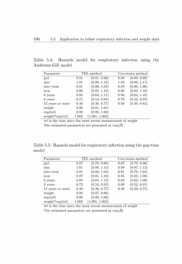
106 5.5. Application to infant respiratory infection and weight data
Table 5.4: Hazards model for respiratory infection using theAndersen-Gill model
Parameter TEL method Cox-strata method
girl 0.91 (0.81, 0.98) 0.89 (0.80, 0.99)zinc 1.01 (0.88, 1.15) 1.02 (0.89, 1.17)zinc+iron 0.91 (0.80, 1.04) 0.93 (0.80, 1.06)iron 0.96 (0.85, 1.10) 0.96 (0.83, 1.10)6 years 0.85 (0.64, 1.11) 0.86 (0.64, 1.16)9 years 0.71 (0.54, 0.94) 0.70 (0.52, 0.95)12 years or more 0.48 (0.30, 0.77) 0.50 (0.30, 0.82)weight 0.96 (0.91, 1.01)exp(tel) 0.99 (0.98, 1.00)weight*exp(tel) 1.002 (1.001, 1.003)
tel is the time since the most recent measurement of weight
The estimated parameters are presented as exp(β)
Table 5.5: Hazards model for respiratory infection using the gap-timemodel
Parameter TEL method Cox-strata method
girl 0.87 (0.79, 0.96) 0.87 (0.79, 0.96)zinc 1.01 (0.88, 1.15) 0.99 (0.87, 1.13)zinc+iron 0.91 (0.80, 1.04) 0.91 (0.79, 1.04)iron 0.97 (0.85, 1.10) 0.95 (0.83, 1.08)6 years 0.85 (0.65, 1.12) 0.82 (0.62, 1.08)9 years 0.72 (0.54, 0.95) 0.69 (0.52, 0.91)12 years or more 0.48 (0.30, 0.77) 0.46 (0.29, 0.75)weight 0.92 (0.87, 0.96)exp(tel) 0.99 (0.99, 1.00)weight*exp(tel) 1.002 (1.001, 1.003)
tel is the time since the most recent measurement of weight
The estimated parameters are presented as exp(β)

5.5. Application to infant respiratory infection and weight data 107
also in this section, the results for the AG model and the gap-timemodel were similar, indicating that an exponential baseline hazardshould be fine. The longitudinal model was specified similarly asin Table 3.9 (random effect growth curve model). The estimate isbased on the joint maximized likelihood of exponential hazard modeland linear random effect model. SAS with the NLMIX procedure(Guo and Carlin, 2004) was used to fit the joint model. With 2,423records of event history data and 3,172 records of longitudinal data,it took 35 hours to fit the model. The result is presented in Table 5.6.
The hazard model in the separate analysis column in Table 5.6is comparable to that of Table 5.5 or Table 3.8 since the exponentialmodel fitted in the joint model also used gap-time as the time scale.The longitudinal model in the separate analysis column is the sameas Table 3.9.
Although small, the estimated risk ratios for the hazard modelgenerally were away from one as compared to the separate model,indicating that the possible frailty effect in the model had been takencare of by the joint model. For the longitudinal model, the randomeffect components were stronger than in the separate model, whichmay indicate that possible under-estimations had been taken careof. The general conclusion for the effect of the variables, however, issimilar to that of separate models.
The significant latent association γ gave additional informationabout the positive association between random effects from bothmodels. In this type of joint model, we may interpret the γ as theeffect of time-dependent frailty in the hazard model which operatesthrough age. The positive value indicates that age had a considerablylarge effect on the hazard of experiencing respiratory infection. Wecompared this finding with an ordinary gap-time Cox-frailty modelusing age as a frailty term. The analysis was performed by adding thefrailty term age in the TEL model of Table 5.5. We found that thevariance of the random effect was 1.03 with a very significant result

108 5.6. Remarks
of LRT (497.6 with 1 degree of freedom) which therefore confirmsthe significant latent association in the joint model.
We summarize the findings for the infants’ respiratory infectionand weight data. Maternal education seemed to be important forinfant respiratory infection but not for weight. Weight was asso-ciated with infant respiratory infection and its duration. Finally,none of the methods show any statistical significance of supplemen-tation. However, we have not considered other important variablessuch as breastfeeding, food intake and socio-economic indicators inthe model, further analyses with those variables may be necessary.
5.6 Remarks
Cox based models such as the LVCF, TEL, and two-stage methodsshould be good enough in situations where data comes a from Cox’smodel with time-dependent covariate. Practically, the TEL methodwould be the first choice. The TEL method may even be used whenthe measurement is only performed once, in this situation the two-stage or the joint model methods may be difficult to perform. TheTEL method is also favorably applied to the switching-treatmenttype covariate where the covariate path is a step function with onlya few values during the period of observation instead of continuousfunction covariate.
Care must be taken in using the Cox based model with a time-dependent covariate under the model with miss-specification. TheCox-strata or Cox-frailty may be more appropriate in the situationwhen the longitudinal covariate is regarded as a nuisance variable,in which there is no need to explicitly estimate their effects. Alter-natively, the joint model method can be used, but this may requirecomplex and heavy computation.
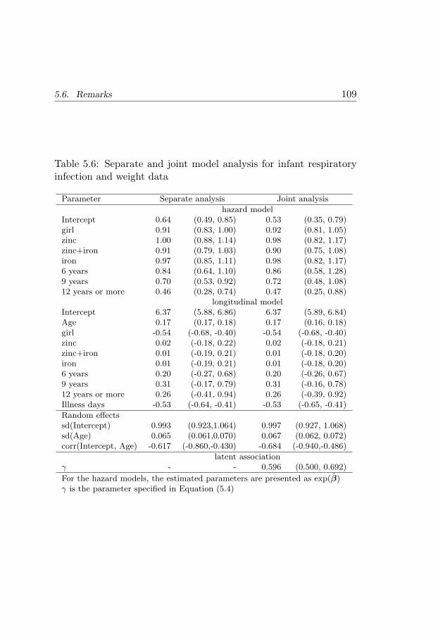
5.6. Remarks 109
Table 5.6: Separate and joint model analysis for infant respiratoryinfection and weight data
Parameter Separate analysis Joint analysis
hazard modelIntercept 0.64 (0.49, 0.85) 0.53 (0.35, 0.79)girl 0.91 (0.83, 1.00) 0.92 (0.81, 1.05)zinc 1.00 (0.88, 1.14) 0.98 (0.82, 1.17)zinc+iron 0.91 (0.79, 1.03) 0.90 (0.75, 1.08)iron 0.97 (0.85, 1.11) 0.98 (0.82, 1.17)6 years 0.84 (0.64, 1.10) 0.86 (0.58, 1.28)9 years 0.70 (0.53, 0.92) 0.72 (0.48, 1.08)12 years or more 0.46 (0.28, 0.74) 0.47 (0.25, 0.88)
longitudinal modelIntercept 6.37 (5.88, 6.86) 6.37 (5.89, 6.84)Age 0.17 (0.17, 0.18) 0.17 (0.16, 0.18)girl -0.54 (-0.68, -0.40) -0.54 (-0.68, -0.40)zinc 0.02 (-0.18, 0.22) 0.02 (-0.18, 0.21)zinc+iron 0.01 (-0.19, 0.21) 0.01 (-0.18, 0.20)iron 0.01 (-0.19, 0.21) 0.01 (-0.18, 0.20)6 years 0.20 (-0.27, 0.68) 0.20 (-0.26, 0.67)9 years 0.31 (-0.17, 0.79) 0.31 (-0.16, 0.78)12 years or more 0.26 (-0.41, 0.94) 0.26 (-0.39, 0.92)Illness days -0.53 (-0.64, -0.41) -0.53 (-0.65, -0.41)
Random effectssd(Intercept) 0.993 (0.923,1.064) 0.997 (0.927, 1.068)sd(Age) 0.065 (0.061,0.070) 0.067 (0.062, 0.072)corr(Intercept, Age) -0.617 (-0.860,-0.430) -0.684 (-0.940,-0.486)
latent associationγ - - 0.596 (0.500, 0.692)
For the hazard models, the estimated parameters are presented as exp(β)γ is the parameter specified in Equation (5.4)

110 5.6. Remarks

Chapter 6
Concluding Remarks
This thesis has contributed several solutions and discussions to theproblems in event history analysis with multiple time scales and lon-gitudinal measurements motivated by some epidemiological studies.
The focus is on the Cox regression model, but this is by no meansthe solution to all problem. Other approaches such as the parametricproportional hazards, additive hazards and accelerated failure times,that have been omitted in the discussion, deserve attention. Simi-lar problems presented in this thesis will certainly appear in thoseapproaches as well.
We have presented methods for choosing the time scale in theCox regression model based on the proportional hazards test andthe frailty model. Although the methods are inferential, we suggestusing the methods as exploratory tools together with considerationof the scientific background of the data.
When several time scales are considered to be important and themodel is a pure bivariate or multivariate time scale model, the Coxmodel with time-dependent strata, or the piecewise constant haz-ards approach are suggested. The price is that, in the Cox model
111

112
with time-dependent strata the effect of the time scale can not bequantified by means of the estimated regression coefficients; and thepiecewise constant hazards is only an approximation of the model.A general methodology for this multivariate time scale problem stillneeds more investigation. The developments since the review by An-dersen et al. (1993, Chapter X) are the non-parametric estimation ofthe bivariate survivor function(Prentice, 1999; Gentleman and Van-dal, 2002) and a more theoretical ground by Ivanoff and Merzbach(2002).
We have presented comparisons of several widely used methodsto deal with longitudinal measurements in the event history analy-sis together with two proposed methods. Comparison by simulationshowed that the time elapsed measurement time method (TEL) per-formed well when the data came from the Cox model with a time-dependent covariate. The two proposed methods based on Cox’smodel with stratification and frailty may be useful when the data aresuspected to cause miss-specification in the Cox model. In the com-parison by simulation we have left out the joint model, a promisingmethod that unfortunately requires heavy and complex computation.The joint model is not in a mature development state yet, especiallyin the computing aspects. Further research is certainly needed. Anestimation method in the generalized linear latent models (Huber,Ronchetti and Victoria-Feser, 2004) seems to be fruitful to estimatethe joint model. Other urgent future research is diagnostic tools forthe joint model, which is still in its infancy.
Finally, any developed methods should have a real advantage inpractice. We have performed several analyses by the discussed meth-ods using epidemiological surveillance and randomized trial data. Wehave confirmed the results obtained by the original investigators andcontributed additional insights to their findings.

Bibliography
Aalen, O. (1978). Nonparametric inference for a family of countingprocesses, The Annals of Statistics 6: 701–726.
Andersen, P. (2003). Two encyclopedia contributions: Time-dependentcovariate, Technical report, Department of Biostatistics, Institute ofPublic Health, University of Copenhagen.
Andersen, P. K. (1991). Survival analysis 1982-1991: The second decadeof the proportional hazards regression model, Statistics in Medicine10: 1931–1941.
Andersen, P. K., Borgan, Ø., Gill, R. D. and Keiding, N. (1993). StatisticalModels Based on Counting Processes, Springer-Verlag Inc.
Andersen, P. K. and Keiding, N. (2002). Multi-state models for eventhistory analysis, Statistical Methods in Medical Research 11(2): 91–115.
Andersen, P. K. and Liestøl, K. (2003). Attenuation caused by infrequentlyupdated covariates in survival analysis, Biostatistics 4: 633–649.
Bailey, K. R. (1984). Asymptotic equivalence between the Cox estimatorand the general ML estimators of regression and survival parametersin the Cox model, The Annals of Statistics 12: 730–736.
Bates, D. M. and Pinheiro, J. (1998). Computational methods for multilevelmodels., Technical memorandum bl0112140-980226-01tm, Bell Labs,Lucent Technologies, Murray Hill, NJ.
113

114 Bibliography
Berzuini, C. and Clayton, D. (1994a). Bayesian analysis of survival onmultiple time scales, Statistics in Medicine 13(8): 823–838.
Berzuini, C. and Clayton, D. (1994b). Bayesian analysis of survival onmultiple time scales, Statistics in Medicine 13: 823–838.
Bhandari, N., Bahl, R., Mazumdar, S., Martines, J., Black, R., Bhan, M.and Infant Feeding Study Group (2003). Effect of community-basedpromotion of exclusive breastfeeding on diarrhoeal illness and growth:A cluster randomised controlled trial, Lancet 361: 1418–1423.
Black, R., Morris, S. and Bryce, J. (2003). Where and why are 10 millionchildren dying every year?, Lancet 361: 2226–2234.
Brostrom, G. (2002). Cox regression; ties without tears, Communicationsin Statistics, Part A – Theory and Methods 31(2): 285–297.
Bruijne, M. H. J. d., Cessie, S. l., Kluin-Nelemans, H. C. and Houwelingen,H. C. v. (2001). On the use of Cox regression in the presence of anirregularly observed time-dependent covariate, Statistics in Medicine20(24): 3817–3829.
Central Bureau of Statistics (CBS) [Indonesia], State Ministry of Popu-lation/National Family Planning Coordinating Board (NFPCB) andMinistry of Health (MOH) and Macro Intemational Inc. (MI) (1998).Indonesia Demographic and Health Survey 1997, CBS and MI.,Calverton, Maryland.
Clayton, D. (1988). The analysis of event history data: A review of progressand outstanding problems, Statistics in Medicine 7: 819–841.
Commenges, D. (1999). Multi-state models in epidemiology, Lifetime DataAnalysis 5: 315–327.
Cox, D. R. (1972). Regression models and life-tables (with discussion),Journal of the Royal Statistical Society, Series B, Methodological34: 187–220.
Cox, D. R. (1975). Partial likelihood, Biometrika 62: 269–276.
Cox, D. R. and Oakes, D. (1984). Analysis of Survival Data, Chapman &Hall Ltd.

Bibliography 115
Danardono (2000). Multilevel Model of the Diarrhea Occurrence in Chil-dren, Master’s thesis, Department of Biostatistics and Demography,Faculty of Public Health Khon Kaen University, Thailand.
Danardono (2003). Event history analysis of childhood mortality and mor-bidity in Purworejo, Indonesia., Statistical studies 30, Department ofStatistics, Umea University.
Diggle, P. (1988). An approach to the analysis of repeated measurements,Biometrics 44: 959–971.
Diggle, P., Heagerty, P., Liang, K.-Y. and Zeger, S. L. (2002). Analysis ofLongitudinal Data, second edn, Oxford University Press.
Do, K.-A. (2002). Biostatistical approaches for modeling longitudinal andevent time data, Clin. Cancer Res. 8(8): 2473–2474.
Doksum, K. A. and Gasko, M. (1990). On a correspondence between modelsin binary regression analysis and in survival analysis, InternationalStatistical Review 58: 243–252.
Duchesne, T. (1999). Multiple Time Scales in Survival Analysis, PhD the-sis, University of Waterloo.
Duchesne, T. and Lawless, J. (2000). Alternative time scales and failuretime models, Lifetime Data Analysis 6(2): 157–179.
Efron, B. (2002). The two-way proportional hazards model, Journal of theRoyal Statistical Society, Series B, Methodological 64(4): 899–909.
Farewell, V. T. and Cox, D. R. (1979). A note on multiple time scales inlife testing, Applied Statistics 28: 73–75.
Faucett, C. L. and Thomas, D. C. (1996). Simultaneously modelling cen-sored survival data and repeatedly measured covariates: A Gibbs sam-pling approach, Statistics in Medicine 15: 1663–1685.
Fleming, T. and Harrington, D. (1991). Counting Processes and SurvivalAnalysis, Wiley.
Fleming, T. and Lin, D. (2000). Survival analysis in clinical trials: Pastdevelopments and future directions, Biometrics. 56(4): 971–983.

116 Bibliography
Gentleman, R. and Vandal, A. C. (2002). Nonparametric estimation of thebivariate CDF for arbitrarily censored data, The Canadian Journal ofStatistics 30(4): 557–571.
Goldstein, H. (1986). Multilevel mixed linear model analysis using iterativegeneralized least squares, Biometrika 73: 43–56.
Goldstein, H. (1989). Restricted unbiased iterative generalized least-squares estimation, Biometrika 76: 622–623.
Grambsch, P. and Therneau, T. (1994). Proportional hazards tests anddiagnostics based on weighted residuals, Biometrika 81: 515–526.
Guo, G. and Rodrıguez, G. (1992). Estimating a multivariate proportionalhazards model for clustered data using the EM algorithm, with anapplication to child survival in Guatemala, Journal of the AmericanStatistical Association 87: 969–976.
Guo, X. and Carlin, B. P. (2004). Separate and joint modeling of longi-tudinal and event time data using standard computer packages, TheAmerican Statistician 58: 16–24.
Hastie, T. J. and Tibshirani, R. J. (1990). Generalized Additive Models,Chapmn and Hall, London.
Hastie, T. and Tibshirani, R. (1986). Generalized additive models, Stat.Sci. 1: 297–318.
Henderson, R., Diggle, P. and Dobson, A. (2000). Joint modelling of longi-tudinal measurements and event time data, Biostatistics 1: 465–480.
Holford, T. (1998). Age-period-cohort analysis, in P. Armitage andT. Colton (eds), Encyclopedia of Biostatistics, John Wiley and Sons,Ltd.
Hosmer, D. and Lemeshow, S. (1999). Applied Survival Analysis. RegressionModeling of Time to Event Data, John Wiley and Sons, Inc.
Hougaard, P. (1995). Frailty models for survival data, Lifetime Data Analy-sis 1: 255–273.

Bibliography 117
Huber, P., Ronchetti, E. and Victoria-Feser, M.-P. (2004). Estimation ofgeneralized linear latent variable models, J. R. Statist. Soc. B 66: 893–908.
Ibrahim, J. G., Chen, M.-H. and Sinha, D. (2001). Bayesian SurvivalAnalysis, Springer-Verlag Inc.
Ihaka, R. and Gentleman, R. (1996). R: A language for data analy-sis and graphics, Journal of Computational and Graphical Statistics5(3): 299–314.
Ivanoff, B. and Merzbach, E. (2002). Random censoring in set-indexedsurvival analysis, The Annals of Applied Probability 12: 944–971.
Jewell, N. and Kalbfleisch, J. (1996). Marker processes in survival analysis,Lifetime Data Analysis 2: 15–29.
Johansen, S. (1983). An extension of Cox’s regression model, InternationalStatistical Review 51: 165–174.
Jones, M. P. and Crowley, J. (1992). Nonparametric tests of the Markovmodel for survival data, Biometrika 79: 513–522.
Kalbfleisch, J. D. and Prentice, R. L. (2002). The Statistical Analysis ofFailure Time Data, second edn, John Wiley and Sons.
Kaplan, E. L. and Meier, P. (1958). Nonparametric estimation from in-complete observations, Journal of the American Statistical Associa-tion 53: 457–481.
Keiding, N. (1990). Statistical inference in the lexis diagram, Phil. Trans.R. Soc. London A 332: 487–509.
Keiding, N. (1999). Event history analysis and inference from observationalepidemiology, Statistics in Medicine 18: 2353–2363.
Kevane, M. and Levine, D. I. (2003). Changing status of daugh-ters in indonesia, Paper c03-126, Center for International and De-velopment Economics Research. University of California, Barkeley.http://Repositories.Cdlib.Org/Iber/Cider/C03-126.

118 Bibliography
Korn, E., Graubard, B. and Midthune, D. (1997). Time-to-event analysisof longitudinal follow-up of a survey: Choice of the time-scale, Am-J-Epidemiol 145: 72–80.
Kuczmarski, R., Ogden, C. and Guo, S. (2002). CDC growth charts for theunited states: Methods and development., Vital Health Stat 11 246,National Center for Health Statistics.
Laird, N. M. and Ware, J. H. (1982). Random-effects models for longitu-dinal data, Biometrics 38: 963–974.
Lee, Y. and Nelder, J. (2001). Hierarchical generalised linear models: Asynthesis of generalised linea models, random-effet models and struc-ture dispersions, Biometrika 88: 987–1006.
Liang, K. and Zeger, S. (1986). Longitudinal data analysis using generalizedlinear models, Biometrika. 73: 13–22.
Liestøl, K. and Andersen, P. (2002). Updating of covariates and choice oftime origin in survival analysis: Problems with vaguely defined diseasestates, Statist. Med. 21: 3701–3714.
Lin, H., McCulloch, C. E. and Mayne, S. T. (2002). Maximum likelihoodestimation in the joint analysis of time-to-event and multiple longitu-dinal variables, Statistics in Medicine 21(16): 2369–2382.
Lin, H., Turnbull, B. W., McCulloch, C. E. and Slate, E. H. (2002). Latentclass models for joint analysis of longitudinal biomarker and eventprocess data: Application to longitudinal prostate-specific antigenreadings and prostate cancer, Journal of the American Statistical As-sociation 97(457): 53–65.
Lind, T. (2004). Iron and Zinc in Infancy: Results from ExperimentalTrials in Sweden and Indonesia, Umea university medical disserta-tions, Epidemiology and Public Health Sciences, Department of PublicHealth and Clinical Medicine, and Pediatrics Department of ClinicalSciences, Umea University, Sweden.
Lindkvist, M. (2000). Added Variable Plots and Influence in Cox’s Regres-sion Model., PhD thesis, Department of Statistics, Umea University.

Bibliography 119
Machfudz, S. (1998). Effect of Morbidity on Change in Mid-upper-armCircumference in Children Under Five Years of Age. a Cohort Studyin Purworejo, Central Java, Indonesia, Master’s thesis, Departmentof Epidemiology and Public Health Umea University.
Manda, S. (2001). A comparison of methods for analysing a nested frailtymodel to child survival in malawi, Australian New Zealand Journal ofStatistics 43(1): 7–16.
McCullagh, P. and Nelder, J. A. (1989). Generalized Linear Models (SecondEdition), Chapman & Hall Ltd.
Mosley, W. and Chen, L. (1984). An analytical framework for the studyof child survival in developing countries, Population and DevelopmentReview 10: 25–48. Suppl.
Ng, E. T. M. and Cook, R. J. (1997). Modeling two-state disease processeswith random effects, Lifetime Data Analysis 3: 315–335.
Oakes, D. (1995). Multiple time scales in survival analysis, Lifetime DataAnalysis 1: 7–18.
Pawitan, Y. and Self, S. (1993). Modeling disease marker processes inAIDS, Journal of the American Statistical Association 88: 719–726.
Pearce, N. (1992). Methodological problems of time-related variables inoccupational cohort studies, Rev Epidemiol Sante Publique 40 Suppl
1: S43–54.
Pebley, A. and Stupp, P. (1987). Reproductive patterns and child mortalityin Guatemala, Demography 24(1): 43–60.
Prentice, R. (1982). Covariate measurement errors and parameter estimatesin a failure time regression model., Biometrika 69: 331–342.
Prentice, R. L. (1989). Surrogate endpoints in clinical trials: Definitionand operational criteria, Statistics in Medicine 8: 431–440.
Prentice, R. L. (1999). On non-parametric maximum likelihood estimationof the bivariate survivor function, Statistics in Medicine 18: 2517–2527.

120 Bibliography
R Development Core Team (2004). R: A language and environment for sta-tistical computing, R Foundation for Statistical Computing, Vienna,Austria. 3-900051-00-3.*http://www.R-project.org
Rabe-Hesketh, S., Yang, S. and Pickles, A. (2001). Multilevel models forcensored and latent responses, Stat. Methods Med. Res. 10: 409–427.
Rice, A., Sacco, L., Hyder, A. and Black, R. (2000). Malnutrition as an un-derlying cause of childhood deaths associated with infectious diseasesin developing countries, Bulletin of the World Health Organization78: 1207–1221.
Robins, J. M. (1986). A new approach to causal inference in mortalitystudies with sustained exposure periods - application to control of thehealthy worker survivor effect, Mathematical Modelling 7: 1393–1512.
Rochon, J. and Gillespie, B. (2001). A methodology for analysing arepeated measures and survival outcome simultaneously., Stat.Med.20(8): 1173–1184.
Sastry, N. (1997). A nested frailty model for survival data, with an appli-cation to the study of child survival in northeast Brazil, Journal ofthe American Statistical Association 92: 426–435.
Scrimshaw, N. S. (2003). Historical concepts of interactions, synergism andantagonism between nutrition and infection, J. Nutr. 133: 316S–321S.
The Cebu Study Team (1991). Underlying and proximate determinants ofchild health: The cebu longitudinal health and nutrition study, Am.J. Epidemiol 133: 185–201.
Therneau, T. M. and Grambsch, P. M. (2000). Modeling Survival Data:Extending the Cox Model, Springer-Verlag Inc.
Trussell, J. and Hammerslough, C. (1983). A hazard-model analysis ofthe covariates of infant and child mortality in sri lanka, Demography20: 1–26.
Tsiatis, A. A. and Davidian, M. (2004). Joint modeling of longitudinal andtime-to-event data: An overview, Statistica Sinica 14: 809–834.

Bibliography 121
Tsiatis, A. A., DeGruttola, V. and Wulfsohn, M. S. (1995). Modeling therelationship of survival to longitudinal data measured with error. Ap-plications to survival and CD4 counts in patients with AIDS, Journalof the American Statistical Association 90: 27–37.
UNICEF (2003). Child Survival and Health. http://www.childinfo.org/eddb/health.htm. Accessed October 13, 2003.
van der Laan, M. J. and Robins, J. M. (2003). Unified Methods for CensoredLongitudinal Data and Causality, Springer-Verlag, Inc.
Vaupel, J. W., Manton, K. G. and Stallard, E. (1979). The impact ofheterogeneity in individual frailty on the dynamics of mortality, De-mography 16: 439–454.
Wahab, A., Winkvist, A., Stenlund, H. and Wilopo, S. (2001). Infantmortality among Indonesian boys and girls: Effect of sibling status,Annals of Tropical Paediatrics 21(1): 66–71.
Wibowo, T. (2000). Does Poor Nutritional Status Lead to Morbidity? ALongitudinal Study of Infants 6 - 12 Months in Purworejo, Centraljava, Indonesia, Master’s thesis, Department of Epidemiology andPublic Health Umea University.
Wilopo, S. and CHN-RL Team (1997). Key Issues on Research Design,Data Collection and Management. Community Health and NutritionResearch Laboratory, Faculty of Medicine, Gadjah Mada University,Reprint Series No. 2, Community Health and Nutrition Research Lab-oratory, Yogyakarta.
Wulfsohn, M. S. and Tsiatis, A. A. (1997). A joint model for survival andlongitudinal data measured with error, Biometrics 53: 330–339.
Xu, J. and Zeger, S. L. (2001). Joint analysis of longitudinal data com-prising repeated measures and times to events, Applied Statistics50(3): 375–387.
Zeger, S. L. and Karim, M. R. (1991). Generalized linear models withrandom effects: A Gibbs sampling approach, Journal of the AmericanStatistical Association 86: 79–86.

122 Bibliography
Zeger, S. L. and Liang, K.-Y. (1986). Longitudinal data analysis for discreteand continuous outcomes, Biometrics 42: 121–130.
Zeger, S. L. and Liang, K.-Y. (1991). Feedback models for discrete andcontinuous time series, Statistica Sinica 1: 51–64.
Zeger, S. L., Liang, K.-Y. and Albert, P. S. (1988). Models for longitu-dinal data: A generalized estimating equation approach, Biometrics44: 1049–1060. (Correction: V45 P347).
Zohoori, N. and Savitz, D. (1997). Econometric approaches to epidemi-ologic data: Relating endogeneity and unobserved heterogeneity toconfounding, Ann. Epidemiol 7: 251–257.

Appendix
123


A-1. Simulating alternative time scale 125
A-1 Simulating alternative time scale
The simulation procedure for the alternative time scales in Section 4.4.1is described here. The true duration T is generated by the ordinary Coxmodel
λ(t | Z) = λ0(t) exp(βZ), t > 0, (A-1)
where λ(t | Z) is the hazard for an individual, λ0(t) is the baseline haz-ard, parametrically specified in this simulation, Z is a zero-one fixed timecovariate with coefficient β.
Z is specified by the Bernoulli distribution with probability 0.4 of suc-cess and the true value of β is 2. The baseline hazards are specified byGompertz, exponential and Weibull hazard functions. Table A-1 showsthe detailed specifications.
Table A-1: The specification of hazard functions and times T gener-ation
Baseline hazard T generation specification
Gompertz λ0(t) = θ1eθ2t T = 1
θ2log(− θ2
θ1
log(u)Ψi
+ 1) θ1 = 0.15,
θ2 = 2
exponential λ0(t) = θ T = −log(u)θΨi
θ = 0.85
Weibull λ0(t) = θ1θ2(θ2t)θ1−1
T = 1θ2
(− log(u)Ψi
)1/θ1 θ1 = 1.2,
θ2 = 0.5
Ψi = exp(βZi), u ∼ U(0, 1)
After T is generated, T1 and T2 are generated by adding δ1 and δ2,respectively. In the simulation, δ1 is U(0, 1) or exponential(0.5); δ2 isU(0.5, 2) or exponential(1.25). Samples of size n = 200 individuals weregenerated according to this procedure with 1000 replications.
A-2 Simulating dual time scales
The simulation procedure for the dual time scales in Section 4.4.2 usedtime-dependent covariate models. In general, if we have a Cox model with

126 A-2. Simulating dual time scales
time dependent covariate
λ(t | Z(t)) = λ0(t)Ψ(β, t), t > 0, (A-2)
the duration T can be generated through the relationship between haz-ard and survival. If T has distribution function F (t) or survival functionS(t) then U = F (T ) or similarly U = S(T ) will follow a uniform U(0, 1)distribution.
Under model (A-2) the cumulative hazard function for T is
G(t) = Λ(t | Z(s), 0 ≤ s ≤ t)
=
∫ t
0
λ0(y)Ψ(β, y)dy (A-3)
so thatS(t) = exp(−G(t)). (A-4)
Now, U = S(T ) is U(0, 1). Therefore, solving U = exp(−G(T )) for Tgives what we want.
Suppose T has hazard function
λ(t | Z(t + δ)) = λ0(t)Ψ(β, t + δ), t > 0, (A-5)
where λ(t | Z(t + δ)) is the hazard function for an individual the covariateprocess Z, λ0(t) is the baseline hazard, parametrically specified in thissimulation, and Ψ(β, t) is specified as
Ψ(β, t) = exp(β1η + β2(t + δ)), t > 0, (A-6)
where β1 and β2 are parameters specified in the simulation, and η and δfollow certain distributions.
The dual times T1 and T2 can be generated from model (A-5) afterspecifying the baseline hazard function λ0. In this simulation, we specifya constant hazard θ such that (A-4) has a closed form solution,
λ(t | Z(t)) = θ exp(β1η + β2(t + δ)), t > 0. (A-7)

A-3. Simulating longitudinal measurements and event-time data 127
The cumulative hazard function for an individual with covariate processZ is
G(t) = Λ(t | Z(s), 0 ≤ s ≤ t)
=
∫ t
0
θ exp(β1η + β2(y + δ))dy
= θeβ1η+β2δ
[eβ2y
β2
]t
y=0
= θeβ1η+β2δ
[eβ2t − 1
β2
]. (A-8)
In the simulation study, we specify a constant hazard θ = 1.2, the truecoefficients β1 = 1.5 , β2 = 0, 1, zero-one fixed covariate η ∼ Bernoulli(p =0.45), and δ follows exponential with rate 0.85 and U(0, 2). Using thisspecification T1 and T2 can be generated through the inverse of G,
G−1(y) =
1
β2log(
β2y
θeβ1η+β2δ + 1)
for β2 6= 0yθe−β1η for β2 = 0
(A-9)
and T1 = G−1(− log(u)) with u ∼ U(0, 1); T2 = T1 + δ. Samples of sizen = 200 individuals were generated according to this procedure with 1000replications.
A-3 Simulating longitudinal measurements
and event-time data
The simulation method in Section 5.4 uses the same principle as in A-2,in which the event times are generated through the inverse of the cumula-tive hazard function. However, in this simulation a longitudinal model isinvolved.
A-3.1 Time-dependent covariate model
This simulation is based on Equations (5.1), (5.2), and (5.3) (Section 5.2).

128 A-3. Simulating longitudinal measurements and event-time data
Specifically we have the longitudinal growth curve model
Y ⋆i (t) = (α1 + a1i) + (α2 + a2i)t, t > 0, i = 1, . . . , n, (A-10)
where Y ⋆i (t) are longitudinal measurements. The random coefficients a1i
and a2i are assumed to follow a bivariate Gaussian distribution with meanzero and variance-covariance matrix Σ.
The measurements are made intermittently for each individual i andwith error, therefore the simulated model for the growth curve is
Yij = Y ⋆i (tij) + ǫij , i = 1, . . . , n, j = 1, . . . ,m, (A-11)
where tij , i = 1, . . . , n, i = 1, . . . ,m are time points of measurement. Themeasurement errors ǫij are assumed to be mutually independent Gaussiandistributed with mean zero and variance σǫ.
The hazard function is modeled as a Cox model with constant baselinehazard
λi(t) = θ exp(β1Zi + β2Y⋆i (t)), t > 0, i = 1, . . . , n. (A-12)
Substituting Y ⋆i (t) from Equation (A-10) and dropping the index i, the
cumulative hazard of (A-12) can be written as
G(t) = Kexp (β2(α2 + a2)t) − 1
β2(α2 + a2), t > 0, (A-13)
where K = θ exp(β1Z + β2α1 + β2a1).The event times are generated by G−1(− log(u)) with u ∼ U(0, 1) (see
(A-9)). Since the simulation is for repeated events, for one individual weassume that the inter event times are generated by the same model butthe time origin is advanced by a certain random amount after each eventtime. In the context of morbidity, we call the advancing of the time origin asduration of illness. For this simulation we choose the lognormal distributionas the distribution of illness duration.
In the simulation, we specified the parameters for the hazard model asθ = 0.4, β1 = 1.2 and varied β2 = 0,−0.1, illness duration was lognormal(0,0.3); and in the growth curve model, we used the parameter values α1 = 6.5,

A-3. Simulating longitudinal measurements and event-time data 129
α2 = 0.17, σǫ = 0.2, and
Σ =
(0.9 −0.04
−0.04 0.01
).
These specified values are roughly equal to the parameter estimates ob-tained from the ZINAK study especially for the weight growth model. Agetime scale is used in the simulation starting from 6 to 12 months, which isalso roughly the same as in the ZINAK study. The counting process styleinput (start, stop], event is used for the repeated events.
The longitudinal measurements were generated at some defined timeintervals. The measurements time points were ti1, ti2, ti3 and were notexactly the same for all individuals. This was done by adding a randomuniform U(−0.4, 0.4) to time points 6, 9, 12 for each individual. Samplesof size n = 50 individuals were generated according to this procedure with500 replications.
A-3.2 Joint model
Simulation of the joint model is based on Equations (5.1), (5.2) and (5.4)(Section 5.2). The procedure for the simulated longitudinal measurementsis similar to that of the time-dependent covariate model with the followingmodification
Yi(t) = (α1 + a1i) + (α2 + a2i)t + α3Zi + ǫi, t > 0, i = 1, . . . , n, (A-14)
where now we have Zi in the model.The simulated event-times were generated from the hazard function
λi(t) = θ exp(β1Zi + β2(a1i + a2it)), t > 0. (A-15)
The cumulative hazard of (A-15) is
G(t) = Kexp (β2a2t) − 1
β2a2
, t > 0, (A-16)
where K = θ exp(β1Z + β2a1). The event times are then generated byG−1(− log(u)) with u ∼ U(0, 1).

130 A-3. Simulating longitudinal measurements and event-time data
The duration of illness, θ, β1, σǫ and Σ, as well as the schedule ofmeasurement times tij were specified similarly as in the time-dependentcovariate model. The α’s were specified as α1 = 6.5, α2 = 0.5, α3 = 1.5and varied β2 = 0, 1. Samples of size n = 50 individuals were generatedaccording to this procedure with 500 replications.

Statistical Studies
issued byDepartment of Statistics, Umea University
SE–901 87 Umea, Sweden
1. Gustafsson, Lennart: Nagra aspekter pa stickprovsteoriervid andliga populationer med tillampningar pa tvastegsurval(1968).
2. Pollak, Kay: Variationsskattningar baserade pa kvadratiskaformer av ordnade variabler, nagra illustrationer (1969).
3. Cassel, Claes-Magnus: Inferensproblemet vid andliga popula-tioner, nagra synpunkter (1970).
4. Wretman, Jan-Hakan: Om inferens vid andliga populationerunder superpopulationsantagande (1970).
5. Carlsson, Olle: Om fordelningen av en summa av vagdaoberoende Poissonvariabler med tillampningar inom statistiskinferensteori och stokastiska processer (1970).
6. Stenlund, Hans och Westlund, Anders: A Monte-Carlo Studyof Some Sampling Designs (1974).
7. Westlund, Anders: Estimation and Prediction InterdependentSystems in the Presence of Specification Errors (1975).
8. Bjornham, Ake och Wiklund, Dan-Erik: Analysis of FetalHeart Rate Variability During Labour: Registration, Estima-tion, and Decision (1976).
9. Hallberg, Bengt: Statistiska modeller for banbrottsfrekvenshos tryckpapper (1976).

10. Freij, Lennart och Wall, Stig: Exploring Child Health and itsEcology (1977).
11. Baudin, Anders: On the Application of Short-term CausalModels (1977).
12. Brannas, Kurt: On Estimation in Economic System in thePresence of Time Varying Parameters (1980).
13. Nyquist, Hans: Recent Studies on Lp-Norm Estimation (1980).
14. Tornkvist, Birgitta: Quantifying Structural Change - A ModelBased Approach (1988).
15. Laitila, Thomas: Estimation in Truncated and Censored Re-gressions (1989).
16. Carlsson, Olle: On Quality Selection (1990).
17. Segerstedt, Bo: On Conditioning and Ridge Estimation inGeneralized Linear Models (1991).
18. Ohman, Marie-Louise: Contributions to Generalized WilcoxonRank Tests (1992).
19. Wiklund, Stig-Johan: Control Charts and Process Adjust-ments (1994).
20. Arnoldsson, Goran: Generalised Linear Models and OptimalDesign (1994).
21. Ohman, Marie-Louise: Aspects of Analysis of Small-SampleRight Censored Data Using Generalized Wilcoxon Rank Tests(1994).
22. Arnoldsson, Goran: Optimal Design for Inference in General-ized Linear Models (1997).

23. Branberg, Kenny: On Test Score Equating (1997).
24. Haggstrom, Jonas: The Minimax Approach to Optimum De-sign of Experiments (2000).
25. Lindkvist, Marie: Added Variable Plots and Influence in Cox’sRegression Model (2000).
26. Pettersson, Hans: Optimum in Average and Minimax Designsfor Estimation of Generalized Linear Models (2001).
27. Haggstrom Lundevaller, Erling: Tests of Random Effects inLinear and Non-Linear Models (2002).
28. Adler, John: Statistical Models for Estimating Career Mobility(2003).
29. Wiberg, Marie: Computerized Achievement Tests - Sequentialand Fixed Length Tests (2003).
30. Danardono: Event History Analysis of Childhood Mortalityand Morbidity in Purworejo, Indonesia (2003).
31. Puu, Margareta: Optimum Experimental Designs for General-ized Linear Models with Multinomial Response (2003).
32. Appelgren, Jari: Locally D-optimal Designs for Bivariate Lo-gistic Regression (2004).
33. Danardono: Multiple Time Scales and Longitudinal Measure-ments in Event History Analysis (2005).
