Multiplicative functionsFrom Wikipedia, the free encyclopedia

Contents

1 Carmichael’s totient function conjecture 11.1 Examples . . . . . . . . . . . . . . . . . . . . . . . . . . . . . . . . . . . . . . . . . . . . . . . 11.2 Lower bounds . . . . . . . . . . . . . . . . . . . . . . . . . . . . . . . . . . . . . . . . . . . . . 11.3 Other results . . . . . . . . . . . . . . . . . . . . . . . . . . . . . . . . . . . . . . . . . . . . . . 11.4 Notes . . . . . . . . . . . . . . . . . . . . . . . . . . . . . . . . . . . . . . . . . . . . . . . . . 21.5 References . . . . . . . . . . . . . . . . . . . . . . . . . . . . . . . . . . . . . . . . . . . . . . . 21.6 External links . . . . . . . . . . . . . . . . . . . . . . . . . . . . . . . . . . . . . . . . . . . . . 2

2 Completely multiplicative function 32.1 Definition . . . . . . . . . . . . . . . . . . . . . . . . . . . . . . . . . . . . . . . . . . . . . . . 32.2 Examples . . . . . . . . . . . . . . . . . . . . . . . . . . . . . . . . . . . . . . . . . . . . . . . 32.3 Properties . . . . . . . . . . . . . . . . . . . . . . . . . . . . . . . . . . . . . . . . . . . . . . . 3

2.3.1 Proof of pseudo-associative property . . . . . . . . . . . . . . . . . . . . . . . . . . . . . 42.3.2 Dirichlet series . . . . . . . . . . . . . . . . . . . . . . . . . . . . . . . . . . . . . . . . 4

2.4 See also . . . . . . . . . . . . . . . . . . . . . . . . . . . . . . . . . . . . . . . . . . . . . . . . 42.5 References . . . . . . . . . . . . . . . . . . . . . . . . . . . . . . . . . . . . . . . . . . . . . . . 4

3 Dedekind psi function 53.1 Higher Orders . . . . . . . . . . . . . . . . . . . . . . . . . . . . . . . . . . . . . . . . . . . . . 53.2 References . . . . . . . . . . . . . . . . . . . . . . . . . . . . . . . . . . . . . . . . . . . . . . 63.3 External links . . . . . . . . . . . . . . . . . . . . . . . . . . . . . . . . . . . . . . . . . . . . . 6

4 Euler’s totient function 74.1 History, terminology, and notation . . . . . . . . . . . . . . . . . . . . . . . . . . . . . . . . . . 84.2 Computing Euler’s totient function . . . . . . . . . . . . . . . . . . . . . . . . . . . . . . . . . . 8

4.2.1 Euler’s product formula . . . . . . . . . . . . . . . . . . . . . . . . . . . . . . . . . . . . 84.2.2 Fourier transform . . . . . . . . . . . . . . . . . . . . . . . . . . . . . . . . . . . . . . . 94.2.3 Divisor sum . . . . . . . . . . . . . . . . . . . . . . . . . . . . . . . . . . . . . . . . . . 94.2.4 Riemann zeta function limit . . . . . . . . . . . . . . . . . . . . . . . . . . . . . . . . . . 10

4.3 Some values of the function . . . . . . . . . . . . . . . . . . . . . . . . . . . . . . . . . . . . . . 114.4 Euler’s theorem . . . . . . . . . . . . . . . . . . . . . . . . . . . . . . . . . . . . . . . . . . . . 114.5 Other formulae involving φ . . . . . . . . . . . . . . . . . . . . . . . . . . . . . . . . . . . . . . 12

4.5.1 Menon’s identity . . . . . . . . . . . . . . . . . . . . . . . . . . . . . . . . . . . . . . . 13

i

ii CONTENTS

4.5.2 Formulae involving the golden ratio . . . . . . . . . . . . . . . . . . . . . . . . . . . . . . 134.6 Generating functions . . . . . . . . . . . . . . . . . . . . . . . . . . . . . . . . . . . . . . . . . . 134.7 Growth of the function . . . . . . . . . . . . . . . . . . . . . . . . . . . . . . . . . . . . . . . . 144.8 Ratio of consecutive values . . . . . . . . . . . . . . . . . . . . . . . . . . . . . . . . . . . . . . 154.9 Totient numbers . . . . . . . . . . . . . . . . . . . . . . . . . . . . . . . . . . . . . . . . . . . . 15

4.9.1 Ford’s theorem . . . . . . . . . . . . . . . . . . . . . . . . . . . . . . . . . . . . . . . . 164.10 Applications . . . . . . . . . . . . . . . . . . . . . . . . . . . . . . . . . . . . . . . . . . . . . . 16

4.10.1 Cyclotomy . . . . . . . . . . . . . . . . . . . . . . . . . . . . . . . . . . . . . . . . . . 164.10.2 The RSA cryptosystem . . . . . . . . . . . . . . . . . . . . . . . . . . . . . . . . . . . . 16

4.11 Unsolved problems . . . . . . . . . . . . . . . . . . . . . . . . . . . . . . . . . . . . . . . . . . 164.11.1 Lehmer’s conjecture . . . . . . . . . . . . . . . . . . . . . . . . . . . . . . . . . . . . . . 164.11.2 Carmichael’s conjecture . . . . . . . . . . . . . . . . . . . . . . . . . . . . . . . . . . . . 17

4.12 See also . . . . . . . . . . . . . . . . . . . . . . . . . . . . . . . . . . . . . . . . . . . . . . . . 174.13 Notes . . . . . . . . . . . . . . . . . . . . . . . . . . . . . . . . . . . . . . . . . . . . . . . . . 174.14 References . . . . . . . . . . . . . . . . . . . . . . . . . . . . . . . . . . . . . . . . . . . . . . . 194.15 External links . . . . . . . . . . . . . . . . . . . . . . . . . . . . . . . . . . . . . . . . . . . . . 20

5 Greatest common divisor 215.1 Overview . . . . . . . . . . . . . . . . . . . . . . . . . . . . . . . . . . . . . . . . . . . . . . . 21

5.1.1 Notation . . . . . . . . . . . . . . . . . . . . . . . . . . . . . . . . . . . . . . . . . . . 215.1.2 Example . . . . . . . . . . . . . . . . . . . . . . . . . . . . . . . . . . . . . . . . . . . 215.1.3 Reducing fractions . . . . . . . . . . . . . . . . . . . . . . . . . . . . . . . . . . . . . . 225.1.4 Coprime numbers . . . . . . . . . . . . . . . . . . . . . . . . . . . . . . . . . . . . . . 225.1.5 A geometric view . . . . . . . . . . . . . . . . . . . . . . . . . . . . . . . . . . . . . . . 22

5.2 Calculation . . . . . . . . . . . . . . . . . . . . . . . . . . . . . . . . . . . . . . . . . . . . . . 225.2.1 Using prime factorizations . . . . . . . . . . . . . . . . . . . . . . . . . . . . . . . . . . 225.2.2 Using Euclid’s algorithm . . . . . . . . . . . . . . . . . . . . . . . . . . . . . . . . . . . 235.2.3 Binary method . . . . . . . . . . . . . . . . . . . . . . . . . . . . . . . . . . . . . . . . 235.2.4 Other methods . . . . . . . . . . . . . . . . . . . . . . . . . . . . . . . . . . . . . . . . 24

5.3 Properties . . . . . . . . . . . . . . . . . . . . . . . . . . . . . . . . . . . . . . . . . . . . . . . 255.4 Probabilities and expected value . . . . . . . . . . . . . . . . . . . . . . . . . . . . . . . . . . . 265.5 The gcd in commutative rings . . . . . . . . . . . . . . . . . . . . . . . . . . . . . . . . . . . . . 265.6 See also . . . . . . . . . . . . . . . . . . . . . . . . . . . . . . . . . . . . . . . . . . . . . . . . 275.7 Notes . . . . . . . . . . . . . . . . . . . . . . . . . . . . . . . . . . . . . . . . . . . . . . . . . 275.8 References . . . . . . . . . . . . . . . . . . . . . . . . . . . . . . . . . . . . . . . . . . . . . . 285.9 Further reading . . . . . . . . . . . . . . . . . . . . . . . . . . . . . . . . . . . . . . . . . . . . 285.10 External links . . . . . . . . . . . . . . . . . . . . . . . . . . . . . . . . . . . . . . . . . . . . . 28

6 Jordan’s totient function 316.1 Definition . . . . . . . . . . . . . . . . . . . . . . . . . . . . . . . . . . . . . . . . . . . . . . . 316.2 Properties . . . . . . . . . . . . . . . . . . . . . . . . . . . . . . . . . . . . . . . . . . . . . . . 316.3 Order of matrix groups . . . . . . . . . . . . . . . . . . . . . . . . . . . . . . . . . . . . . . . . 32

CONTENTS iii

6.4 Examples . . . . . . . . . . . . . . . . . . . . . . . . . . . . . . . . . . . . . . . . . . . . . . . 326.5 Notes . . . . . . . . . . . . . . . . . . . . . . . . . . . . . . . . . . . . . . . . . . . . . . . . . 326.6 References . . . . . . . . . . . . . . . . . . . . . . . . . . . . . . . . . . . . . . . . . . . . . . . 336.7 External links . . . . . . . . . . . . . . . . . . . . . . . . . . . . . . . . . . . . . . . . . . . . . 33

7 Lehmer’s totient problem 347.1 Properties . . . . . . . . . . . . . . . . . . . . . . . . . . . . . . . . . . . . . . . . . . . . . . . 347.2 References . . . . . . . . . . . . . . . . . . . . . . . . . . . . . . . . . . . . . . . . . . . . . . . 347.3 External links . . . . . . . . . . . . . . . . . . . . . . . . . . . . . . . . . . . . . . . . . . . . . 35

8 Liouville function 368.1 Series . . . . . . . . . . . . . . . . . . . . . . . . . . . . . . . . . . . . . . . . . . . . . . . . . 368.2 Conjectures . . . . . . . . . . . . . . . . . . . . . . . . . . . . . . . . . . . . . . . . . . . . . . 368.3 References . . . . . . . . . . . . . . . . . . . . . . . . . . . . . . . . . . . . . . . . . . . . . . . 37

9 Multiplicative function 419.1 Examples . . . . . . . . . . . . . . . . . . . . . . . . . . . . . . . . . . . . . . . . . . . . . . . 419.2 Properties . . . . . . . . . . . . . . . . . . . . . . . . . . . . . . . . . . . . . . . . . . . . . . . 429.3 Convolution . . . . . . . . . . . . . . . . . . . . . . . . . . . . . . . . . . . . . . . . . . . . . . 43

9.3.1 Dirichlet series for some multiplicative functions . . . . . . . . . . . . . . . . . . . . . . 439.4 Multiplicative function over F [X] . . . . . . . . . . . . . . . . . . . . . . . . . . . . . . . . . . . 43

9.4.1 Zeta function and Dirichlet series in F [X] . . . . . . . . . . . . . . . . . . . . . . . . . . 449.5 See also . . . . . . . . . . . . . . . . . . . . . . . . . . . . . . . . . . . . . . . . . . . . . . . . 449.6 References . . . . . . . . . . . . . . . . . . . . . . . . . . . . . . . . . . . . . . . . . . . . . . . 449.7 External links . . . . . . . . . . . . . . . . . . . . . . . . . . . . . . . . . . . . . . . . . . . . . 44

10 Möbius function 4510.1 Definition . . . . . . . . . . . . . . . . . . . . . . . . . . . . . . . . . . . . . . . . . . . . . . . 4510.2 Properties and applications . . . . . . . . . . . . . . . . . . . . . . . . . . . . . . . . . . . . . . 45

10.2.1 Properties . . . . . . . . . . . . . . . . . . . . . . . . . . . . . . . . . . . . . . . . . . 4610.2.2 Mertens function . . . . . . . . . . . . . . . . . . . . . . . . . . . . . . . . . . . . . . . 4610.2.3 Applications . . . . . . . . . . . . . . . . . . . . . . . . . . . . . . . . . . . . . . . . . 47

10.3 Recurrence . . . . . . . . . . . . . . . . . . . . . . . . . . . . . . . . . . . . . . . . . . . . . . 4810.4 Matrix inverse . . . . . . . . . . . . . . . . . . . . . . . . . . . . . . . . . . . . . . . . . . . . . 4810.5 Average order . . . . . . . . . . . . . . . . . . . . . . . . . . . . . . . . . . . . . . . . . . . . . 4910.6 μ(n) sections . . . . . . . . . . . . . . . . . . . . . . . . . . . . . . . . . . . . . . . . . . . . . . 4910.7 Generalizations . . . . . . . . . . . . . . . . . . . . . . . . . . . . . . . . . . . . . . . . . . . . 49

10.7.1 Incidence algebras . . . . . . . . . . . . . . . . . . . . . . . . . . . . . . . . . . . . . . . 4910.7.2 Popovici’s function . . . . . . . . . . . . . . . . . . . . . . . . . . . . . . . . . . . . . . 49

10.8 Physics . . . . . . . . . . . . . . . . . . . . . . . . . . . . . . . . . . . . . . . . . . . . . . . . . 4910.9 See also . . . . . . . . . . . . . . . . . . . . . . . . . . . . . . . . . . . . . . . . . . . . . . . . 5010.10Notes . . . . . . . . . . . . . . . . . . . . . . . . . . . . . . . . . . . . . . . . . . . . . . . . . 5010.11References . . . . . . . . . . . . . . . . . . . . . . . . . . . . . . . . . . . . . . . . . . . . . . . 50

iv CONTENTS

10.12External links . . . . . . . . . . . . . . . . . . . . . . . . . . . . . . . . . . . . . . . . . . . . . 51

11 Radical of an integer 5211.1 Examples . . . . . . . . . . . . . . . . . . . . . . . . . . . . . . . . . . . . . . . . . . . . . . . 5211.2 Properties . . . . . . . . . . . . . . . . . . . . . . . . . . . . . . . . . . . . . . . . . . . . . . . 5211.3 See also . . . . . . . . . . . . . . . . . . . . . . . . . . . . . . . . . . . . . . . . . . . . . . . . 5311.4 References . . . . . . . . . . . . . . . . . . . . . . . . . . . . . . . . . . . . . . . . . . . . . . . 53

12 Ramanujan tau function 5412.1 Values . . . . . . . . . . . . . . . . . . . . . . . . . . . . . . . . . . . . . . . . . . . . . . . . . 5412.2 Ramanujan’s conjectures . . . . . . . . . . . . . . . . . . . . . . . . . . . . . . . . . . . . . . . 5512.3 Congruences for the tau function . . . . . . . . . . . . . . . . . . . . . . . . . . . . . . . . . . . 5512.4 Conjectures on τ(n) . . . . . . . . . . . . . . . . . . . . . . . . . . . . . . . . . . . . . . . . . . 5512.5 Notes . . . . . . . . . . . . . . . . . . . . . . . . . . . . . . . . . . . . . . . . . . . . . . . . . 5612.6 References . . . . . . . . . . . . . . . . . . . . . . . . . . . . . . . . . . . . . . . . . . . . . . . 56

13 Unit function 5713.1 See also . . . . . . . . . . . . . . . . . . . . . . . . . . . . . . . . . . . . . . . . . . . . . . . . 5713.2 References . . . . . . . . . . . . . . . . . . . . . . . . . . . . . . . . . . . . . . . . . . . . . . . 5713.3 Text and image sources, contributors, and licenses . . . . . . . . . . . . . . . . . . . . . . . . . . 58

13.3.1 Text . . . . . . . . . . . . . . . . . . . . . . . . . . . . . . . . . . . . . . . . . . . . . . 5813.3.2 Images . . . . . . . . . . . . . . . . . . . . . . . . . . . . . . . . . . . . . . . . . . . . 5913.3.3 Content license . . . . . . . . . . . . . . . . . . . . . . . . . . . . . . . . . . . . . . . . 60

Chapter 1

Carmichael’s totient function conjecture

In mathematics, Carmichael’s totient function conjecture concerns the multiplicity of values of Euler’s totientfunction φ(n), which counts the number of integers less than and coprime to n. It states that, for every n there is atleast one other integer m ≠ n such that φ(m) = φ(n). Robert Carmichael first stated this conjecture in 1907, but as atheorem rather than as a conjecture. However, his proof was faulty and in 1922 he retracted his claim and stated theconjecture as an open problem.

1.1 Examples

The totient function φ(n) is equal to 2 when n is one of the three values 3, 4, and 6. Thus, if we take any one of thesethree values as n, then either of the other two values can be used as the m for which φ(m) = φ(n).Similarly, the totient is equal to 4 when n is one of the four values 5, 8, 10, and 12, and it is equal to 6 when n is oneof the four values 7, 9, 14, and 18. In each case, there is more than one value of n having the same value of φ(n).The conjecture states that this phenomenon of repeated values holds for every n.

1.2 Lower bounds

There are very high lower bounds for Carmichael’s conjecture that are relatively easy to determine. Carmichaelhimself proved that any counterexample to his conjecture (that is, a value n such that φ(n) is different from thetotients of all other numbers) must be at least 1037, and Victor Klee extended this result to 10400. A lower bound of1010

7 was given by Schlafly and Wagon, and a lower bound of 101010 was determined by Kevin Ford in 1998.[1]

The computational technique underlying these lower bounds depends on some key results of Klee that make it pos-sible to show that the smallest counterexample must be divisible by squares of the primes dividing its totient value.Klee’s results imply that 8 and Fermat primes (primes of the form 2k+1) excluding 3 do not divide the smallest coun-terexample. Consequently, proving the conjecture is equivalent to proving that the conjecture holds for all integerscongruent to 4 (mod 8).

1.3 Other results

Ford also proved that if there exists a counterexample to the Conjecture, then a positive fraction (that is infinitelymany) of the integers are likewise counterexamples.[1]

Although the conjecture is widely believed, Carl Pomerance gave a sufficient condition for an integer n to be a coun-terexample to the conjecture (Pomerance 1974). According to this condition, n is a counterexample if for everyprime p such that p − 1 divides φ(n), p2 divides n. However Pomerance showed that the existence of such an integeris highly improbable. Essentially, one can show that if the first k primes p congruent to 1 (mod q) (where q is a prime)are all less than qk+1, then such an integer will be divisible by every prime and thus cannot exist. In any case, proving

1

2 CHAPTER 1. CARMICHAEL’S TOTIENT FUNCTION CONJECTURE

that Pomerance’s counterexample does not exist is far from proving Carmichael’s Conjecture. However if it existsthen infinitely many counterexamples exist as asserted by Ford.Another way of stating Carmichael’s conjecture is that, if A(f) denotes the number of positive integers n for whichφ(n) = f, then A(f) can never equal 1. Relatedly, Wacław Sierpiński conjectured that every positive integer otherthan 1 occurs as a value of A(f), a conjecture that was proven in 1999 by Kevin Ford.[2]

1.4 Notes[1] Sándor & Crstici (2004) p.228

[2] Sándor & Crstici (2004) p.229

1.5 References• Carmichael, R. D. (1907), “On Euler’s φ-function”, Bulletin of the American Mathematical Society 13 (5):241–243, doi:10.1090/S0002-9904-1907-01453-2, MR 1558451.

• Carmichael, R. D. (1922), “Note on Euler’s φ-function”, Bulletin of the American Mathematical Society 28 (3):109–110, doi:10.1090/S0002-9904-1922-03504-5, MR 1560520.

• Ford, K. (1999), “The number of solutions of φ(x) =m",Annals ofMathematics 150 (1): 283–311, doi:10.2307/121103,JSTOR 121103, MR 1715326, Zbl 0978.11053.

• Guy, Richard K. (2004), Unsolved problems in number theory (3rd ed.), Springer-Verlag, B39, ISBN 978-0-387-20860-2, Zbl 1058.11001.

• Klee, V. L., Jr. (1947), “On a conjecture of Carmichael”, Bulletin of the American Mathematical Society 53(12): 1183–1186, doi:10.1090/S0002-9904-1947-08940-0, MR 0022855, Zbl 0035.02601.

• Pomerance, Carl (1974), “On Carmichael’s conjecture” (PDF), Proceedings of the American MathematicalSociety 43 (2): 297–298, doi:10.2307/2038881, Zbl 0254.10009.

• Sándor, Jozsef; Crstici, Borislav (2004), Handbook of number theory II, Dordrecht: Kluwer Academic, pp.228–229, ISBN 1-4020-2546-7, Zbl 1079.11001.

• Schlafly, A.; Wagon, S. (1994), “Carmichael’s conjecture on the Euler function is valid below 1010,000,000",Mathematics of Computation 63 (207): 415–419, doi:10.2307/2153585, JSTOR 2153585, MR 1226815, Zbl0801.11001.

1.6 External links• Weisstein, Eric W., “Carmichael’s Totient Function Conjecture”, MathWorld.

Chapter 2

Completely multiplicative function

In number theory, functions of positive integers which respect products are important and are called completelymultiplicative functions or totally multiplicative functions. A weaker condition is also important, respecting onlyproducts of coprime numbers, and such functions are called multiplicative functions. Outside of number theory, theterm “multiplicative function” is often taken to be synonymous with “completely multiplicative function” as definedin this article.

2.1 Definition

A completely multiplicative function (or totally multiplicative function) is an arithmetic function (that is, a func-tion whose domain is the natural numbers), such that f(1) = 1 and f(ab) = f(a) f(b) holds for all positive integers aand b.[1]

Without the requirement that f(1) = 1, one could still have f(1) = 0, but then f(a) = 0 for all positive integers a, sothis is not a very strong restriction.The definition above can be rephrased using the language of algebra: A completely multiplicative function is anendomorphism of the monoid (Z+, ·) , that is, the positive integers under multiplication.

2.2 Examples

The easiest example of a completelymultiplicative function is amonomial with leading coefficient 1: For any particularpositive integer n, define f(a) = an. Then f(bc) = (bc)n = bncn = f(b)f(c), and f(1) = 1n = 1.The Liouville function is a non-trivial example of a completely multiplicative function as are Dirichlet characters.

2.3 Properties

A completely multiplicative function is completely determined by its values at the prime numbers, a consequence ofthe fundamental theorem of arithmetic. Thus, if n is a product of powers of distinct primes, say n = pa qb ..., thenf(n) = f(p)a f(q)b ...While the Dirichlet convolution of two multiplicative functions is multiplicative, the Dirichlet convolution of twocompletely multiplicative functions need not be completely multiplicative.There are a variety of statements about a function which are equivalent to it being completely multiplicative. Forexample, if a function f multiplicative then is completely multiplicative if and only if the Dirichlet inverse is µfwhere µ is the Möbius function.[2]

Completely multiplicative functions also satisfy a pseudo-associative law. If f is completely multiplicative thenf · (g ∗ h) = (f · g) ∗ (f · h)

3

4 CHAPTER 2. COMPLETELY MULTIPLICATIVE FUNCTION

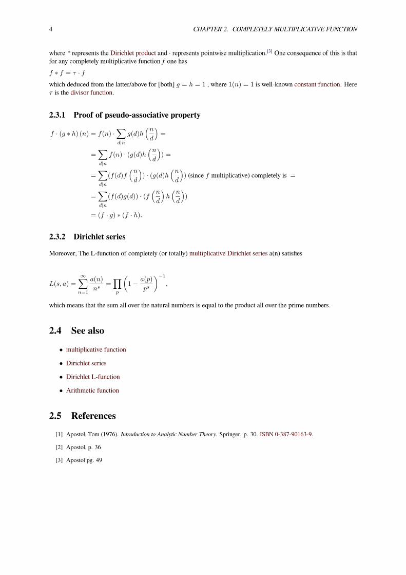
where * represents the Dirichlet product and · represents pointwise multiplication.[3] One consequence of this is thatfor any completely multiplicative function f one hasf ∗ f = τ · fwhich deduced from the latter/above for [both] g = h = 1 , where 1(n) = 1 is well-known constant function. Hereτ is the divisor function.

2.3.1 Proof of pseudo-associative property

f · (g ∗ h) (n) = f(n) ·∑d|n

g(d)h(nd

)=

=∑d|n

f(n) · (g(d)h(nd

)) =

=∑d|n

(f(d)f(nd

)) · (g(d)h

(nd

)) (since f multiplicative) completely is =

=∑d|n

(f(d)g(d)) · (f(nd

)h(nd

))

= (f · g) ∗ (f · h).

2.3.2 Dirichlet series

Moreover, The L-function of completely (or totally) multiplicative Dirichlet series a(n) satisfies

L(s, a) =

∞∑n=1

a(n)

ns=

∏p

(1− a(p)

ps

)−1

,

which means that the sum all over the natural numbers is equal to the product all over the prime numbers.

2.4 See also• multiplicative function

• Dirichlet series

• Dirichlet L-function

• Arithmetic function

2.5 References[1] Apostol, Tom (1976). Introduction to Analytic Number Theory. Springer. p. 30. ISBN 0-387-90163-9.

[2] Apostol, p. 36

[3] Apostol pg. 49

Chapter 3

Dedekind psi function

In number theory, the Dedekind psi function is the multiplicative function on the positive integers defined by

ψ(n) = n∏p|n

(1 +

1

p

),

where the product is taken over all primes p dividing n (by convention, ψ(1) is the empty product and so has value1). The function was introduced by Richard Dedekind in connection with modular functions.The value of ψ(n) for the first few integers n is:

1, 3, 4, 6, 6, 12, 8, 12, 12, 18, 12, 24 ... (sequence A001615 in OEIS).

ψ(n) is greater than n for all n greater than 1, and is even for all n greater than 2. If n is a square-free number thenψ(n) = σ(n).The ψ function can also be defined by setting ψ(pn) = (p+1)pn-1 for powers of any prime p, and then extending thedefinition to all integers by multiplicativity. This also leads to a proof of the generating function in terms of theRiemann zeta function, which is

∑ ψ(n)

ns=ζ(s)ζ(s− 1)

ζ(2s).

This is also a consequence of the fact that we can write as a Dirichlet convolution of ψ = Id ∗ |µ| .

3.1 Higher Orders

The generalization to higher orders via ratios of Jordan’s totient is

ψk(n) =J2k(n)

Jk(n)

with Dirichlet series

∑n≥1

ψk(n)

ns=ζ(s)ζ(s− k)

ζ(2s)

It is also the Dirichlet convolution of a power and the square of the Möbius function,

5

6 CHAPTER 3. DEDEKIND PSI FUNCTION

ψk(n) = nk ∗ µ2(n)

If

ϵ2 = 1, 0, 0, 1, 0, 0, 0, 0, 1, 0, 0, 0, 0, 0, 0, 1, 0, 0, 0 . . .

is the characteristic function of the squares, another Dirichlet convolution leads to the generalized σ-function,

ϵ2(n) ∗ ψk(n) = σk(n)

3.2 References• Goro Shimura (1971). Introduction to the Arithmetic Theory of Automorphic Functions. Princeton. (page 25,equation (1))

• Carella, N. A. (2010). “Squarefree Integers AndExtremeValuesOf SomeArithmetic Functions”. arXiv:1012.4817.

• Mathar, Richard J. (2011). “Survey ofDirichlet series ofmultiplicative arithmetic functions”. arXiv:1106.4038.Section 3.13.2

• A065958 is ψ2, A065959 is ψ3, and A065960 is ψ4

3.3 External links• Weisstein, Eric W., “Dedekind Function”, MathWorld.

Chapter 4

Euler’s totient function

For other functions named after Euler, see List of things named after Leonhard Euler. For other functions namedphi, see phi.In number theory, Euler’s totient function (or Euler’s phi function), denoted as φ(n) or ϕ(n), is an arithmetic

The first thousand values of φ(n)

function that counts the positive integers less than or equal to n that are relatively prime to n. (These integers aresometimes referred to as totatives of n.) Thus, if n is a positive integer, then φ(n) is the number of integers k in therange 1 ≤ k ≤ n for which the greatest common divisor gcd(n, k) = 1.[1][2]

Euler’s totient function is a multiplicative function, meaning that if two numbers m and n are coprime, then φ(mn) =φ(m) φ(n).[3][4]

For example, let n = 9. Then gcd(9, 3) = gcd(9, 6) = 3 and gcd(9, 9) = 9. The other six numbers in the range 1 ≤ k ≤9, that is 1, 2, 4, 5, 7 and 8 are relatively prime to 9. Therefore, φ(9) = 6. As another example, φ(1) = 1 since gcd(1,1) = 1.

7

8 CHAPTER 4. EULER’S TOTIENT FUNCTION

Euler’s phi function is important mainly because it gives the order of the multiplicative group of integers modulo n(the group of units of the ring ℤ/nℤ).[5] It also plays a key role in the definition of the RSA encryption system.

4.1 History, terminology, and notation

Leonhard Euler introduced the function in 1763.[6][7][8] However, he did not at that time choose any specific sym-bol to denote it. In a 1784 publication, Euler studied the function further, choosing the Greek letter π to denoteit: he wrote πD for “the multitude of numbers less than D, and which have no common divisor with it”.[9] Thestandard notation[7][10] φ(A) comes from Gauss's 1801 treatise Disquisitiones Arithmeticae.[11] However, Gauss didn'tuse parentheses around the argument and wrote φA. Thus, it is often called Euler’s phi function or simply the phifunction.In 1879, J. J. Sylvester coined the term totient for this function,[12][13] so it is also referred to as Euler’s totientfunction, the Euler totient, or Euler’s totient. Jordan’s totient is a generalization of Euler’s.The cototient of n is defined as n – φ(n), i.e. the number of positive integers less than or equal to n that are divisibleby at least one prime that also divides n.

4.2 Computing Euler’s totient function

There are several formulas for computing φ(n).

4.2.1 Euler’s product formula

It states

φ(n) = n∏p|n

(1− 1

p

),

where the product is over the distinct prime numbers dividing n. (The notation is described in the article Arithmeticalfunction.)The proof of Euler’s product formula depends on two important facts.

1) The function φ(n) is multiplicative

This means that if gcd(m, n) = 1, then φ(mn) = φ(m) φ(n). (Sketch of proof: let A, B, C be the sets of residueclasses modulo-and-coprime to m, n, mn respectively; then there is a bijection between A × B and C, by the Chineseremainder theorem.)

2) φ(pk) = pk − pk−1 = pk−1(p − 1)

That is, if p is prime and k ≥ 1 then

φ(pk) = pk − pk−1 = pk−1(p− 1) = pk(1− 1

p

).

Proof: since p is a prime number the only possible values of gcd(pk, m) are 1, p, p2, ..., pk, and the only way forgcd(pk, m) to not equal 1 is for m to be a multiple of p. The multiples of p that are less than or equal to pk are p, 2p,3p, ..., pk − 1p = pk, and there are pk − 1 of them. Therefore, the other pk − pk − 1 numbers are all relatively prime to pk.

4.2. COMPUTING EULER’S TOTIENT FUNCTION 9

Proof of Euler’s product formula

The fundamental theorem of arithmetic states that if n > 1 there is a unique expression for n,

n = pk11 · · · pkr

r ,

where p1 < p2 < ... < pr are prime numbers and each ki ≥ 1. (The case n = 1 corresponds to the empty product.)Repeatedly using the multiplicative property of φ and the formula for φ(pk) gives

φ(n) = φ(pk11 )φ(pk2

2 ) · · ·φ(pkrr )

= pk11

(1− 1

p1

)pk22

(1− 1

p2

)· · · pkr

r

(1− 1

pr

)= pk1

1 pk22 · · · pkr

r

(1− 1

p1

)(1− 1

p2

)· · ·

(1− 1

pr

)= n

(1− 1

p1

)(1− 1

p2

)· · ·

(1− 1

pr

).

This is Euler’s product formula.

Example

φ(36) = φ(2232

)= 36

(1− 1

2

)(1− 1

3

)= 36 · 1

2· 23= 12.

In words, this says that the distinct prime factors of 36 are 2 and 3; half of the thirty-six integers from 1 to 36 aredivisible by 2, leaving eighteen; a third of those are divisible by 3, leaving twelve numbers that are coprime to 36.And indeed there are twelve positive integers that are coprime with 36 and lower than 36: 1, 5, 7, 11, 13, 17, 19, 23,25, 29, 31, and 35.

4.2.2 Fourier transform

The totient is the discrete Fourier transform of the gcd, evaluated at 1: (Schramm (2008))

F x [m] =n∑

k=1

xk · e−2πimkn , xk = gcd(k, n) for k ∈ 1 . . . n

φ(n) = F x [1] =n∑

k=1

gcd(k, n)e−2πi kn .

The real part of this formula is

φ(n) =n∑

k=1

gcd(k, n) cos 2π kn.

Note that unlike the other two formulae (the Euler product and the divisor sum) this one does not require knowing thefactors of n. However, it does involve the calculation of the greatest common divisor of n and every positive integerless than n, which would suffice to provide the factorization anyway.

4.2.3 Divisor sum

The property established by Gauss,[14] that

10 CHAPTER 4. EULER’S TOTIENT FUNCTION

∑d|n

φ(d) = n,

where the sum is over all positive divisors d of n, can be proven in several ways. (see Arithmetical function fornotational conventions.)One way is to note that φ(d) is also equal to the number of possible generators of the cyclic group Cd; specifically,if Cd = <g>, then gk is a generator for every k coprime to d. Since every element of Cn generates a cyclic subgroup,and all subgroups of Cd ≤ Cn are generated by some element of Cn, the formula follows.[15] In the article Root ofunity Euler’s formula is derived by using this argument in the special case of the multiplicative group of the nth rootsof unity.This formula can also be derived in a more concrete manner.[16] Let n = 20 and consider the fractions between 0 and1 with denominator 20:

120 ,

220 ,

320 ,

420 ,

520 ,

620 ,

720 ,

820 ,

920 ,

1020 ,

1120 ,

1220 ,

1320 ,

1420 ,

1520 ,

1620 ,

1720 ,

1820 ,

1920 ,

2020

Put them into lowest terms:

120 ,

110 ,

320 ,

15 ,

14 ,

310 ,

720 ,

25 ,

920 ,

12 ,

1120 ,

35 ,

1320 ,

710 ,

34 ,

45 ,

1720 ,

910 ,

1920 ,

11

First note that all the divisors of 20 are denominators. And second, note that there are 20 fractions. Which fractionshave 20 as denominator? The ones whose numerators are relatively prime to 20

(120 ,

320 ,

720 ,

920 ,

1120 ,

1320 ,

1720 ,

1920

).

By definition this is φ(20) fractions. Similarly, there are φ(10) = 4 fractions with denominator 10(

110 ,

310 ,

710 ,

910

),

φ(5) = 4 fractions with denominator 5(15 ,

25 ,

35 ,

45

), and so on.

In detail, we're considering the fractions of the form k/n where k is an integer from 1 to n inclusive. Upon reducingthese to lowest terms, each fraction will have as its denominator some divisor of n. We can group the fractions togetherby denominator, and we must show that for a given divisor d of n, the number of such fractions with denominator dis φ(d).Note that to reduce k/n to lowest terms, we divide the numerator and denominator by gcd(k, n). The reduced fractionswith denominator d are therefore precisely the ones originally of the form k/n in which gcd(k, n)=n/d. The questiontherefore becomes: how many k are there less than or equal to n which verify gcd(k, n)=n/d? Any such kmust clearlybe a multiple of n/d, but it must also be coprime to d (if it had any common divisor s with d, then sn/d would be alarger common divisor of n and k). Conversely, any multiple k of n/d which is coprime to d will satisfy gcd(n, k)=n/d.We can generate φ(d) such numbers by taking the numbers less than d coprime to d and multiplying each one by n/d(these products will of course each by smaller than n, as required). This in fact generates all such numbers, as if kis a multiple of n/d coprime to d (and less than n), then k/(n/d) will still be coprime to d, and must also be smallerthan d, else k would be larger than n. Thus there are precisely φ(d) values of k less than or equal to n such that gcd(k,n)=n/d, which was to be demonstrated.Möbius inversion gives

φ(n) =∑d|n

d · µ(nd

)= n

∑d|n

µ(d)

d,

where μ is the Möbius function.

This formula may also be derived from the product formula by multiplying out∏

p|n

(1− 1

p

)to get

∑d|n

µ(d)d .

4.2.4 Riemann zeta function limit

For n > 1 the Euler totient function can be calculated as a limit involving the Riemann zeta function:

φ(n) = n lims→1

ζ(s)∑d|n

µ(d)(e1/d)(s−1)

4.3. SOME VALUES OF THE FUNCTION 11

whereζ(s) is the Riemann zeta function, µ is the Möbius function, e is e (mathematical constant), and d is a divisor.

4.3 Some values of the function

The first 99 values (sequence A000010 in OEIS) are shown in the table and graph below:[17]

Graph of the first 100 values

The top line in the graph, y = n − 1, is a true upper bound. It is attained whenever n is prime. There is no lower boundthat is a straight line of positive slope; no matter how gentle the slope of a line is, there will eventually be points ofthe plot below the line. More precisely, the lower limit of the graph is proportional to n/log log n rather than beinglinear.[18]

4.4 Euler’s theorem

Main article: Euler’s theorem

This states that if a and n are relatively prime then

aφ(n) ≡ 1 mod n.

The special case where n is prime is known as Fermat’s little theorem.This follows from Lagrange’s theorem and the fact that φ(n) is the order of the multiplicative group of integers modulon.

12 CHAPTER 4. EULER’S TOTIENT FUNCTION

The RSA cryptosystem is based on this theorem: it implies that the inverse of the function a 7→ ae mod n , wheree is the (public) encryption exponent, is the function b 7→ bd mod n , where d , the (private) decryption exponent,is the multiplicative inverse of e modulo φ(n) . The difficulty of computing φ(n) without knowing the factorizationof n is thus the difficulty of computing d : this is known as the RSA problem which can be solved by factoring n. The owner of the private key knows the factorization, since an RSA private key is constructed by choosing n asthe product of two (randomly chosen) large primes p and q . Only n is publicly disclosed, and given the difficulty tofactor large numbers we have the guarantee that no-one else knows the factorization.

4.5 Other formulae involving φ

• a | b implies φ(a) | φ(b).

• n | φ(an − 1) (a, n > 1)

• φ(mn) = φ(m)φ(n) · dφ(d) where d = gcd(m, n). Note the special cases

• φ(2m) =

2φ(m) ifmeven isφ(m) ifmodd is

and

• φ (nm) = nm−1φ(n).

• φ(lcm(m,n)) · φ(gcd(m,n)) = φ(m) · φ(n).

Compare this to the formula lcm(m,n) · gcd(m,n) = m · n. (See lcm).

• φ(n) is even for n ≥ 3.Moreover, if n has r distinct odd prime factors, 2r | φ(n).

• For any a > 1 and n > 6 such that 4 ∤ n there exists an l ≥ 2n such that l | φ(an − 1) .

•∑

d|nµ2(d)φ(d) = n

φ(n)[19]

•∑

1≤k≤n(k,n)=1

k = 12nφ(n) for n > 1

•∑n

k=1 φ(k) =12

(1 +

∑nk=1 µ(k)

⌊nk

⌋2)= 3

π2n2 +O

(n(logn)2/3(log logn)4/3

)([20] cited in [21])

•∑n

k=1φ(k)k =

∑nk=1

µ(k)k

⌊nk

⌋= 6

π2n+O((logn)2/3(log logn)4/3

) [20]

•∑n

k=1k

φ(k) =315ζ(3)2π4 n− logn

2 +O((logn)2/3

) [22]

•∑n

k=11

φ(k) =315ζ(3)2π4

(logn+ γ −

∑pprime

log pp2−p+1

)+O

((logn)2/3

n

)[23]

(here γ is the Euler constant).

•∑

1≤k≤n(k,m)=1

1 = nφ(m)m +O

(2ω(m)

),

wherem > 1 is a positive integer and ω(m) is the number of distinct prime factors ofm. (a, b) is a standard abbreviationfor gcd(a, b).[24]

4.6. GENERATING FUNCTIONS 13

4.5.1 Menon’s identity

Main article: Menon’s identity

In 1965 P. Kesava Menon proved

∑1≤k≤n

gcd(k,n)=1

gcd(k − 1, n) = φ(n)d(n),

where d(n) = σ0(n) is the number of divisors of n.

4.5.2 Formulae involving the golden ratio

Schneider[25] found a pair of identities connecting the totient function, the golden ratio and the Möbius function µ(n). In this section φ(n) is the totient function, and ϕ = 1+

√5

2 = 1.618 . . . is the golden ratio.They are:

ϕ = −∞∑k=1

φ(k)

klog

(1− 1

ϕk

)and

1

ϕ= −

∞∑k=1

µ(k)

klog

(1− 1

ϕk

).

Subtracting them gives

∞∑k=1

µ(k)− φ(k)

klog

(1− 1

ϕk

)= 1.

Applying the exponential function to both sides of the preceding identity yields an infinite product formula for Euler’snumber e

e =

∞∏k=1

(1− 1

ϕk

)µ(k)−φ(k)k

.

The proof is based on the formulae

∑∞k=1

φ(k)k (− log(1− xk)) = x

1−x and∑∞

k=1µ(k)k (− log(1− xk)) = x, valid for 0 < x < 1.

4.6 Generating functions

The Dirichlet series for φ(n) may be written in terms of the Riemann zeta function as:[26]

∞∑n=1

φ(n)

ns=ζ(s− 1)

ζ(s).

The Lambert series generating function is[27]

14 CHAPTER 4. EULER’S TOTIENT FUNCTION

∞∑n=1

φ(n)qn

1− qn=

q

(1− q)2

which converges for |q| < 1.Both of these are proved by elementary series manipulations and the formulae for φ(n).

4.7 Growth of the function

In the words of Hardy & Wright, the order of φ(n) is “always ‘nearly n’.”[28]

First[29]

lim sup φ(n)n

= 1,

but as n goes to infinity,[30] for all δ > 0

φ(n)

n1−δ→ ∞.

These two formulae can be proved by using little more than the formulae for φ(n) and the divisor sum function σ(n).In fact, during the proof of the second formula, the inequality

6

π2<φ(n)σ(n)

n2< 1,

true for n > 1, is proven.We also have[18]

lim inf φ(n)n

log logn = e−γ .

Here γ is Euler’s constant, γ = 0.577215665..., eγ = 1.7810724..., e−γ = 0.56145948... .Proving this doesn't quite require the prime number theorem.[31][32] Since log log (n) goes to infinity, this formulashows that

lim inf φ(n)n

= 0.

In fact, more is true.[33][34]

φ(n) > neγ log logn+ 3

log lognfor n > 2, and

φ(n) < neγ log logn for infinitely many n.

The second inequality was shown by Jean-Louis Nicolas. Ribenboim says “The method of proof is interesting, in thatthe inequality is shown first under the assumption that the Riemann hypothesis is true, secondly under the contraryassumption.”[34]

For the average order, we have[20][35]

4.8. RATIO OF CONSECUTIVE VALUES 15

φ(1) + φ(2) + · · ·+ φ(n) =3n2

π2+O

(n(logn)2/3(log logn)4/3

)(n→ ∞),

due to ArnoldWalfisz, its proof exploiting estimates on exponential sums due to I. M. Vinogradov and N.M. Korobov(this is currently the best known estimate of this type). The “Big O” stands for a quantity that is bounded by a constanttimes the function of “n” inside the parentheses (which is small compared to n2).This result can be used to prove[36] that the probability of two randomly chosen numbers being relatively prime is 6

π2 .

4.8 Ratio of consecutive values

In 1950 Somayajulu proved[37][38]

lim inf φ(n+1)φ(n) = 0 and

lim sup φ(n+1)φ(n) = ∞.

In 1954 Schinzel and Sierpiński strengthened this, proving[37][38] that the set

φ(n+ 1)

φ(n), n = 1, 2, · · ·

is dense in the positive real numbers. They also proved[37] that the set

φ(n)

n, n = 1, 2, · · ·

is dense in the interval (0, 1).

4.9 Totient numbers

A totient number is a value of Euler’s totient function: that is, an m for which there is at least one n for which φ(n)= m. The valency or multiplicity of a totient numberm is the number of solutions to this equation.[39] A nontotient is anatural number which is not a totient number: there are infinitely many nontotients,[40] and indeed every odd numberhas an even multiple which is a nontotient.[41]

The number of totient numbers up to a given limit x is

x

logx exp((C + o(1))(log log logx)2

)for a constant C = 0.8178146... .[42]

If counted accordingly to multiplicity, the number of totient numbers up to a given limit x is

|n : ϕ(n) ≤ x| = ζ(2)ζ(3)

ζ(6)· x+R(x)

where the error term R is of order at most x/(logx)k for any positive k.[43]

It is known that the multiplicity of m exceeds mδ infinitely often for any δ < 0.55655.[44][45]

16 CHAPTER 4. EULER’S TOTIENT FUNCTION

4.9.1 Ford’s theorem

Ford (1999) proved that for every integer k ≥ 2 there is a totient number m of multiplicity k: that is, for which theequation φ(n) = m has exactly k solutions; this result had previously been conjectured by Wacław Sierpiński,[46] andit had been obtained as a consequence of Schinzel’s hypothesis H.[42] Indeed, each multiplicity that occurs, does soinfinitely often.[42][45]

However, no number m is known with multiplicity k = 1. Carmichael’s totient function conjecture is the statementthat there is no such m.[47]

4.10 Applications

4.10.1 Cyclotomy

Main article: Constructible polygon

In the last section of theDisquisitiones[48][49] Gauss proves[50] that a regular n-gon can be constructed with straightedgeand compass if φ(n) is a power of 2. If n is a power of an odd prime number the formula for the totient says its totientcan be a power of two only if a) n is a first power and b) n − 1 is a power of 2. The primes that are one more than apower of 2 are called Fermat primes, and only five are known: 3, 5, 17, 257, and 65537. Fermat and Gauss knew ofthese. Nobody has been able to prove whether there are any more.Thus, a regular n-gon has a straightedge-and-compass construction if n is a product of distinct Fermat primes andany power of 2. The first few such n are[51] 2, 3, 4, 5, 6, 8, 10, 12, 15, 16, 17, 20, 24, 30, 32, 34, 40, ... . (sequenceA003401 in OEIS)

4.10.2 The RSA cryptosystem

Main article: RSA (algorithm)

Setting up an RSA system involves choosing large prime numbers p and q, computing n = pq and k = φ(n), and findingtwo numbers e and d such that ed ≡ 1 (mod k). The numbers n and e (the “encryption key”) are released to the public,and d (the “decryption key”) is kept private.A message, represented by an integer m, where 0 < m < n, is encrypted by computing S = me (mod n).It is decrypted by computing t = Sd (mod n). Euler’s Theorem can be used to show that if 0 < t < n, then t = m.The security of an RSA systemwould be compromised if the number n could be factored or if φ(n) could be computedwithout factoring n.

4.11 Unsolved problems

4.11.1 Lehmer’s conjecture

Main article: Lehmer’s totient problem

If p is prime, then φ(p) = p − 1. In 1932 D. H. Lehmer asked if there are any composite numbers n such that φ(n) |n − 1. None are known.[52]

In 1933 he proved that if any such n exists, it must be odd, square-free, and divisible by at least seven primes (i.e.ω(n) ≥ 7). In 1980 Cohen and Hagis proved that n > 1020 and that ω(n) ≥ 14.[53] Further, Hagis showed that if 3divides n then n > 101937042 and ω(n) ≥ 298848.[54][55]

4.12. SEE ALSO 17

4.11.2 Carmichael’s conjecture

Main article: Carmichael’s totient function conjecture

This states that there is no number n with the property that for all other numbers m, m ≠ n, φ(m) ≠ φ(n). See Ford’stheorem above.As stated in the main article, if there is a single counterexample to this conjecture, there must be infinitely manycounterexamples, and the smallest one has at least ten billion digits in base 10.[39]

4.12 See also

• Carmichael function

• Duffin–Schaeffer conjecture

• Generalizations of Fermat’s little theorem

• Highly composite number

• Multiplicative group of integers modulo n

• Ramanujan sum

4.13 Notes[1] Long (1972, p. 85)

[2] Pettofrezzo & Byrkit (1970, p. 72)

[3] Long (1972, p. 162)

[4] Pettofrezzo & Byrkit (1970, p. 80)

[5] See Euler’s theorem.

[6] L. Euler "Theoremata arithmetica nova methodo demonstrata" (An arithmetic theorem proved by a new method), Novicommentarii academiae scientiarum imperialis Petropolitanae (NewMemoirs of the Saint-Petersburg Imperial Academy ofSciences), 8 (1763), 74-104. (The work was presented at the Saint-Petersburg Academy on October 15, 1759. A workwith the same title was presented at the Berlin Academy on June 8, 1758). Available on-line in: Ferdinand Rudio, ed.,Leonhardi Euleri Commentationes Arithmeticae, volume 1, in: Leonhardi Euleri Opera Omnia, series 1, volume 2 (Leipzig,Germany, B. G. Teubner, 1915), pages 531-555. On page 531, Euler defines n as the number of integers that are smallerthan N and relatively prime to N (… aequalis sit multitudini numerorum ipso N minorum, qui simul ad eum sint primi,…), which is the phi function, φ(N).

[7] Sandifer, p. 203

[8] Graham et al. p. 133 note 111

[9] L. Euler, Speculationes circa quasdam insignes proprietates numerorum, Acta Academiae Scientarum Imperialis Petropoliti-nae, vol. 4, (1784), pp. 18-30, or Opera Omnia, Series 1, volume 4, pp. 105-115. (The work was presented at theSaint-Petersburg Academy on October 9, 1775).

[10] Both φ(n) and ϕ(n) are seen in the literature. These are two forms of the lower-case Greek letter phi.

[11] Gauss, Disquisitiones Arithmeticae article 38

[12] J. J. Sylvester (1879) “On certain ternary cubic-form equations”, American Journal of Mathematics, 2 : 357-393; Sylvestercoins the term “totient” on page 361.

[13] “totient”. Oxford English Dictionary (2nd ed.). Oxford University Press. 1989.

[14] Gauss, DA, art 39

18 CHAPTER 4. EULER’S TOTIENT FUNCTION

[15] Gauss, DA art. 39, arts. 52-54

[16] Graham et al. pp. 134-135

[17] The cell for n = 0 in the upper-left corner of the table is empty, as the function φ(n) is commonly defined only for positiveintegers, so it is not defined for n = 0.

[18] Hardy & Wright 1979, thm. 328

[19] Dineva (in external refs), prop. 1

[20] Walfisz, Arnold (1963). Weylsche Exponentialsummen in der neueren Zahlentheorie. Mathematische Forschungsberichte(in German) 16. Berlin: VEB Deutscher Verlag der Wissenschaften. Zbl 0146.06003.

[21] Lomadse, G., “The scientific work of Arnold Walfisz” (PDF), Acta Arithmetica 10 (3): 227–237

[22] R. Sitaramachandrarao. On an error term of Landau II, Rocky Mountain J. Math. 15 (1985), 579-588

[23] Also R. Sitaramachandrarao (loc. cit.)

[24] Bordellès in the external links

[25] All formulae in the section are from Schneider (in the external links)

[26] Hardy & Wright 1979, thm. 288

[27] Hardy & Wright 1979, thm. 309

[28] Hardy & Wright 1979, intro to § 18.4

[29] Hardy & Wright 1979, thm. 326

[30] Hardy & Wright 1979, thm. 327

[31] In fact Chebychev’s theorem (Hardy & Wright 1979, thm.7) and Mertens’ third theorem is all that’s needed

[32] Hardy & Wright 1979, thm. 436

[33] Bach & Shallit, thm. 8.8.7

[34] Ribenboim, The Book of Prime Number Records, Section 4.I.C

[35] Sándor, Mitrinović & Crstici (2006) pp.24-25

[36] Hardy & Wright 1979, thm. 332

[37] Ribenboim, p.38

[38] Sándor, Mitrinović & Crstici (2006) p.16

[39] Guy (2004) p.144

[40] Sándor & Crstici (2004) p.230

[41] Zhang, Mingzhi (1993). “On nontotients”. Journal of Number Theory 43 (2): 168–172. doi:10.1006/jnth.1993.1014.ISSN 0022-314X. Zbl 0772.11001.

[42] Ford, Kevin (1998). “The distribution of totients”. Ramanujan J. 2 (1-2): 67–151. doi:10.1007/978-1-4757-4507-8_8.ISSN 1382-4090. Zbl 0914.11053.

[43] Sándor et al (2006) p.22

[44] Sándor et al (2006) p.21

[45] Guy (2004) p.145

[46] Sándor & Crstici (2004) p.229

[47] Sándor & Crstici (2004) p.228

[48] Gauss, DA. The 7th § is arts. 336-366

[49] Gauss proved if n satisfies certain conditions then the n-gon can be constructed. In 1837 PierreWantzel proved the converse,if the n-gon is constructible, then n must satisfy Gauss’s conditions

4.14. REFERENCES 19

[50] Gauss, DA, art 366

[51] Gauss, DA, art. 366. This list is the last sentence in the Disquisitiones

[52] Ribenboim, pp. 36-37.

[53] Cohen, Graeme L.; Hagis, Peter, jun. (1980). “On the number of prime factors of n if φ(n) divides n−1”. Nieuw Arch.Wiskd., III. Ser. 28: 177–185. ISSN 0028-9825. Zbl 0436.10002.

[54] Hagis, Peter, jun. (1988). “On the equation M⋅φ(n)=n−1”. Nieuw Arch. Wiskd., IV. Ser. 6 (3): 255–261. ISSN 0028-9825. Zbl 0668.10006.

[55] Guy (2004) p.142

4.14 References

TheDisquisitiones Arithmeticae has been translated fromLatin into English andGerman. TheGerman edition includesall of Gauss’ papers on number theory: all the proofs of quadratic reciprocity, the determination of the sign of theGauss sum, the investigations into biquadratic reciprocity, and unpublished notes.References to the Disquisitiones are of the form Gauss, DA, art. nnn.

• Abramowitz, M.; Stegun, I. A. (1964), Handbook of Mathematical Functions, New York: Dover Publications,ISBN 0-486-61272-4. See paragraph 24.3.2.

• Bach, Eric; Shallit, Jeffrey (1996), Algorithmic Number Theory (Vol I: Efficient Algorithms), MIT Press Seriesin the Foundations of Computing, Cambridge, MA: The MIT Press, ISBN 0-262-02405-5, Zbl 0873.11070

• Ford, Kevin (1999), “The number of solutions of φ(x) = m", Annals of Mathematics 150 (1): 283–311,doi:10.2307/121103, ISSN 0003-486X, JSTOR 121103, MR 1715326, Zbl 0978.11053.

• Gauss, Carl Friedrich; Clarke, Arthur A. (translator into English) (1986), Disquisitiones Arithmeticae (Second,corrected edition), New York: Springer, ISBN 0-387-96254-9

• Gauss, Carl Friedrich; Maser, H. (translator into German) (1965), Untersuchungen uber hohere Arithmetik(Disquisitiones Arithmeticae & other papers on number theory) (Second edition), New York: Chelsea, ISBN0-8284-0191-8

• Graham, Ronald; Knuth, Donald; Patashnik, Oren (1994), Concrete Mathematics: a foundation for computerscience (2nd ed.), Reading, MA: Addison-Wesley, ISBN 0-201-55802-5, Zbl 0836.00001

• Guy, Richard K. (2004),Unsolved Problems in Number Theory, Problem Books inMathematics (3rd ed.), NewYork, NY: Springer-Verlag, ISBN 0-387-20860-7, Zbl 1058.11001

• Hardy, G. H.; Wright, E. M. (1979), An Introduction to the Theory of Numbers (Fifth ed.), Oxford: OxfordUniversity Press, ISBN 978-0-19-853171-5

• Long, Calvin T. (1972), Elementary Introduction to Number Theory (2nd ed.), Lexington: D. C. Heath andCompany, LCCN 77-171950

• Pettofrezzo, Anthony J.; Byrkit, Donald R. (1970), Elements of Number Theory, Englewood Cliffs: PrenticeHall, LCCN 77-81766

• Ribenboim, Paulo (1996), The New Book of Prime Number Records (3rd ed.), New York: Springer, ISBN0-387-94457-5, Zbl 0856.11001

• Sandifer, Charles (2007), The early mathematics of Leonhard Euler, MAA, ISBN 0-88385-559-3

• Sándor, József; Mitrinović, Dragoslav S.; Crstici, Borislav, eds. (2006), Handbook of number theory I, Dor-drecht: Springer-Verlag, pp. 9–36, ISBN 1-4020-4215-9, Zbl 1151.11300

• Sándor, Jozsef; Crstici, Borislav (2004). Handbook of number theory II. Dordrecht: Kluwer Academic. pp.179–327. ISBN 1-4020-2546-7. Zbl 1079.11001.

• Schramm, Wolfgang (2008), “The Fourier transform of functions of the greatest common divisor”, ElectronicJournal of Combinatorial Number Theory A50 (8(1)).

20 CHAPTER 4. EULER’S TOTIENT FUNCTION

4.15 External links• Hazewinkel, Michiel, ed. (2001), “Totient function”, Encyclopedia of Mathematics, Springer, ISBN 978-1-55608-010-4

• Kirby Urner, Computing totient function in Python and scheme, (2003)

• Euler’s Phi Function and the Chinese Remainder Theorem — proof that Φ(n) is multiplicative

• Euler’s totient function calculator in JavaScript — up to 20 digits

• Bordellès, Olivier, Numbers prime to q in [1, n]

• Dineva, Rosica, The Euler Totient, the Möbius, and the Divisor Functions

• Miyata, Daisuke & Yamashita, Michinori, Derived logarithmic function of Euler’s function

• Plytage, Loomis, Polhill Summing Up The Euler Phi Function

• Schneider, Robert P. A Golden Product Identity for e.

Chapter 5

Greatest common divisor

In mathematics, the greatest common divisor (gcd) of two or more integers, when at least one of them is not zero,is the largest positive integer that divides the numbers without a remainder. For example, the GCD of 8 and 12 is4.[1][2]

The GCD is also known as the greatest common factor (gcf),[3] highest common factor (hcf),[4] greatest commonmeasure (gcm),[5] or highest common divisor.[6]

This notion can be extended to polynomials (see Polynomial greatest common divisor) and other commutative rings(see below).

5.1 Overview

5.1.1 Notation

In this article we will denote the greatest common divisor of two integers a and b as gcd(a,b).Some textbooks use (a,b).[1][2][6][7]

The J (programming language) uses a +. b

5.1.2 Example

The number 54 can be expressed as a product of two integers in several different ways:

54× 1 = 27× 2 = 18× 3 = 9× 6.

Thus the divisors of 54 are:

1, 2, 3, 6, 9, 18, 27, 54.

Similarly the divisors of 24 are:

1, 2, 3, 4, 6, 8, 12, 24.

The numbers that these two lists share in common are the common divisors of 54 and 24:

1, 2, 3, 6.

The greatest of these is 6. That is the greatest common divisor of 54 and 24. One writes:

21

22 CHAPTER 5. GREATEST COMMON DIVISOR

gcd(54, 24) = 6.

5.1.3 Reducing fractions

The greatest common divisor is useful for reducing fractions to be in lowest terms. For example, gcd(42, 56) = 14,therefore,

42

56=

3 · 144 · 14

=3

4.

5.1.4 Coprime numbers

Two numbers are called relatively prime, or coprime, if their greatest common divisor equals 1. For example, 9 and28 are relatively prime.

5.1.5 A geometric view

For example, a 24-by-60 rectangular area can be divided into a grid of: 1-by-1 squares, 2-by-2 squares, 3-by-3squares, 4-by-4 squares, 6-by-6 squares or 12-by-12 squares. Therefore, 12 is the greatest common divisor of 24 and60. A 24-by-60 rectangular area can be divided into a grid of 12-by-12 squares, with two squares along one edge(24/12 = 2) and five squares along the other (60/12 = 5).

5.2 Calculation

5.2.1 Using prime factorizations

Greatest common divisors can in principle be computed by determining the prime factorizations of the two numbersand comparing factors, as in the following example: to compute gcd(18, 84), we find the prime factorizations 18 = 2· 32 and 84 = 22 · 3 · 7 and notice that the “overlap” of the two expressions is 2 · 3; so gcd(18, 84) = 6. In practice,this method is only feasible for small numbers; computing prime factorizations in general takes far too long.Here is another concrete example, illustrated by a Venn diagram. Suppose it is desired to find the greatest commondivisor of 48 and 180. First, find the prime factorizations of the two numbers:

48 = 2 × 2 × 2 × 2 × 3,180 = 2 × 2 × 3 × 3 × 5.

What they share in common is two “2"s and a “3":

2

2

2

23

53

5.2. CALCULATION 23

Least common multiple = 2 × 2 × ( 2 × 2 × 3 ) × 3 × 5 = 720Greatest common divisor = 2 × 2 × 3 = 12.

5.2.2 Using Euclid’s algorithm

A much more efficient method is the Euclidean algorithm, which uses a division algorithm such as long division incombination with the observation that the gcd of two numbers also divides their difference. To compute gcd(48,18),divide 48 by 18 to get a quotient of 2 and a remainder of 12. Then divide 18 by 12 to get a quotient of 1 and aremainder of 6. Then divide 12 by 6 to get a remainder of 0, which means that 6 is the gcd. Note that we ignoredthe quotient in each step except to notice when the remainder reached 0, signalling that we had arrived at the answer.Formally the algorithm can be described as:

gcd(a, 0) = a

gcd(a, b) = gcd(b, amod b)where

amod b = a− b⌊ab

⌋If the arguments are both greater than zero then the algorithm can be written in more elementary terms as follows:

gcd(a, a) = a

gcd(a, b) = gcd(a− b, b) , if a > bgcd(a, b) = gcd(a, b− a) , if b > a

Complexity of Euclidean method

The existence of the Euclidean algorithm places (the decision problem version of) the greatest common divisor prob-lem in P, the class of problems solvable in polynomial time. The GCD problem is not known to be in NC, and so thereis no known way to parallelize its computation across many processors; nor is it known to be P-complete, which wouldimply that it is unlikely to be possible to parallelize GCD computation. In this sense the GCD problem is analogousto e.g. the integer factorization problem, which has no known polynomial-time algorithm, but is not known to beNP-complete. Shallcross et al. showed that a related problem (EUGCD, determining the remainder sequence arisingduring the Euclidean algorithm) is NC-equivalent to the problem of integer linear programming with two variables;if either problem is inNC or is P-complete, the other is as well.[8] SinceNC contains NL, it is also unknown whethera space-efficient algorithm for computing the GCD exists, even for nondeterministic Turing machines.Although the problem is not known to be inNC, parallel algorithms asymptotically faster than the Euclidean algorithmexist; the best known deterministic algorithm is by Chor and Goldreich, which (in the CRCW-PRAM model) cansolve the problem in O(n/log n) time with n1+ε processors.[9] Randomized algorithms can solve the problem in O((logn)2) time on exp

[O(√n logn

)]processors (note this is superpolynomial).[10]

5.2.3 Binary method

An alternative method of computing the gcd is the binary gcd method which uses only subtraction and division by 2.In outline the method is as follows: Let a and b be the two non negative integers. Also set the integer d to 0. Thereare five possibilities:

• a = b.

As gcd(a, a) = a, the desired gcd is a×2d (as a and b are changed in the other cases, and d records the number oftimes that a and b have been both divided by 2 in the next step, the gcd of the initial pair is the product of a by 2d).

24 CHAPTER 5. GREATEST COMMON DIVISOR

• Both a and b are even.

In this case 2 is a common divisor. Divide both a and b by 2, increment d by 1 to record the number of times 2 is acommon divisor and continue.

• a is even and b is odd.

In this case 2 is not a common divisor. Divide a by 2 and continue.

• a is odd and b is even.

As in the previous case 2 is not a common divisor. Divide b by 2 and continue.

• Both a and b are odd.

As gcd(a,b) = gcd(b,a) and we have already considered the case a = b, we may assume that a > b. The number c = a− b is smaller than a yet still positive. Any number that divides a and b must also divide c so every common divisorof a and b is also a common divisor of b and c Similarly, a = b + c and every common divisor of b and c is also acommon divisor of a and b. So the two pairs (a, b) and (b, c) have the same common divisors, and thus gcd(a,b) =gcd(b,c). Moreover, as a and b are both odd, c is even, and one may replace c by c/2 without changing the gcd. Thusthe process can be continued with the pair (a, b) replaced by the smaller numbers (c/2, b).Each of the above steps reduces at least one of a and b towards 0 and so can only be repeated a finite number oftimes. Thus one must eventually reach the case a = b, which is the only stopping case. Then, as quoted above, thegcd is a×2d.This algorithm may easily programmed as follows:Input: a, b positive integers Output: g and d such that g is odd and gcd(a, b) = g×2d d := 0 while a and b are botheven do a := a/2 b := b/2 d := d + 1 while a ≠ b do if a is even then a := a/2 else if b is even then b := b/2 else if a> b then a := (a – b)/2 else b := (b – a)/2 g := a output g, dExample: (a, b, d) = (48, 18, 0) → (24, 9, 1) → (12, 9, 1) → (6, 9, 1) → (3, 9, 1) → (3, 6, 1) → (3, 3, 1) ; the originalgcd is thus 2d = 21 times a= b= 3, that is 6.The Binary GCD algorithm is particularly easy to implement on binary computers. The test for whether a number isdivisible by two can be performed by testing the lowest bit in the number. Division by two can be achieved by shiftingthe input number by one bit. Each step of the algorithm makes at least one such shift. Subtracting two numberssmaller than a and b costs O(log a+ log b) bit operations. Each step makes at most one such subtraction. The totalnumber of steps is at most the sum of the numbers of bits of a and b, hence the computational complexity is

O((log a+ log b)2)

For further details see Binary GCD algorithm.

5.2.4 Other methods

If a and b are both nonzero, the greatest common divisor of a and b can be computed by using least common multiple(lcm) of a and b:

gcd(a, b) = a · blcm(a, b)

but more commonly the lcm is computed from the gcd.Using Thomae’s function f,

gcd(a, b) = af

(b

a

),

5.3. PROPERTIES 25

which generalizes to a and b rational numbers or commensurable real numbers.Keith Slavin has shown that for odd a ≥ 1:

gcd(a, b) = log2a−1∏k=0

(1 + e−2iπkb/a)

which is a function that can be evaluated for complex b.[11] Wolfgang Schramm has shown that

gcd(a, b) =a∑

k=1

exp(2πikb/a) ·∑d|a

cd(k)

d

is an entire function in the variable b for all positive integers a where cd(k) is Ramanujan’s sum.[12] Donald Knuthproved the following reduction:

gcd(2a − 1, 2b − 1) = 2gcd(a,b) − 1

for non-negative integers a and b, where a and b are not both zero.[13] More generally

gcd(na − 1, nb − 1) = ngcd(a,b) − 1

which can be proven by considering the Euclidean algorithm in base n. Another useful identity relates gcd(a, b) tothe Euler’s totient function:

gcd(a, b) =∑

k|a and k|b

φ(k).

5.3 Properties• Every common divisor of a and b is a divisor of gcd(a, b).

• gcd(a, b), where a and b are not both zero, may be defined alternatively and equivalently as the smallest positiveinteger d which can be written in the form d = a·p + b·q, where p and q are integers. This expression is calledBézout’s identity. Numbers p and q like this can be computed with the extended Euclidean algorithm.

• gcd(a, 0) = |a|, for a ≠ 0, since any number is a divisor of 0, and the greatest divisor of a is |a|.[2][6] This isusually used as the base case in the Euclidean algorithm.

• If a divides the product b·c, and gcd(a, b) = d, then a/d divides c.

• If m is a non-negative integer, then gcd(m·a, m·b) = m·gcd(a, b).

• If m is any integer, then gcd(a + m·b, b) = gcd(a, b).

• If m is a nonzero common divisor of a and b, then gcd(a/m, b/m) = gcd(a, b)/m.

• The gcd is a multiplicative function in the following sense: if a1 and a2 are relatively prime, then gcd(a1·a2, b)= gcd(a1, b)·gcd(a2, b). In particular, recalling that gcd is a positive integer valued function (i.e., gets naturalvalues only) we obtain that gcd(a, b·c) = 1 if and only if gcd(a, b) = 1 and gcd(a, c) = 1.

• The gcd is a commutative function: gcd(a, b) = gcd(b, a).

• The gcd is an associative function: gcd(a, gcd(b, c)) = gcd(gcd(a, b), c).

• The gcd of three numbers can be computed as gcd(a, b, c) = gcd(gcd(a, b), c), or in some different way byapplying commutativity and associativity. This can be extended to any number of numbers.

26 CHAPTER 5. GREATEST COMMON DIVISOR

• gcd(a, b) is closely related to the least common multiple lcm(a, b): we have

gcd(a, b)·lcm(a, b) = a·b.This formula is often used to compute least common multiples: one first computes the gcd with Euclid’salgorithm and then divides the product of the given numbers by their gcd.

• The following versions of distributivity hold true:

gcd(a, lcm(b, c)) = lcm(gcd(a, b), gcd(a, c))lcm(a, gcd(b, c)) = gcd(lcm(a, b), lcm(a, c)).

• It is sometimes useful to define gcd(0, 0) = 0 and lcm(0, 0) = 0 because then the natural numbers become acomplete distributive lattice with gcd as meet and lcm as join operation.[14] This extension of the definition isalso compatible with the generalization for commutative rings given below.

• In a Cartesian coordinate system, gcd(a, b) can be interpreted as the number of segments between points withintegral coordinates on the straight line segment joining the points (0, 0) and (a, b).

5.4 Probabilities and expected value

In 1972, James E. Nymann showed that k integers, chosen independently and uniformly from 1,...,n, are coprimewith probability 1/ζ(k) as n goes to infinity, where ζ refers to the Riemann zeta function.[15] (See coprime for aderivation.) This result was extended in 1987 to show that the probability that k random integers have greatestcommon divisor d is d−k/ζ(k).[16]

Using this information, the expected value of the greatest common divisor function can be seen (informally) to notexist when k = 2. In this case the probability that the gcd equals d is d−2/ζ(2), and since ζ(2) = π2/6 we have

E(2) =∞∑d=1

d6

π2d2=

6

π2

∞∑d=1

1

d.

This last summation is the harmonic series, which diverges. However, when k ≥ 3, the expected value is well-defined,and by the above argument, it is

E(k) =∞∑d=1

d1−kζ(k)−1 =ζ(k − 1)

ζ(k).

For k = 3, this is approximately equal to 1.3684. For k = 4, it is approximately 1.1106.

5.5 The gcd in commutative rings

See also: divisor (ring theory)

The notion of greatest common divisor can more generally be defined for elements of an arbitrary commutative ring,although in general there need not exist one for every pair of elements.If R is a commutative ring, and a and b are in R, then an element d of R is called a common divisor of a and b if itdivides both a and b (that is, if there are elements x and y in R such that d·x = a and d·y = b). If d is a common divisorof a and b, and every common divisor of a and b divides d, then d is called a greatest common divisor of a and b.Note that with this definition, two elements a and b may very well have several greatest common divisors, or noneat all. If R is an integral domain then any two gcd’s of a and b must be associate elements, since by definition eitherone must divide the other; indeed if a gcd exists, any one of its associates is a gcd as well. Existence of a gcd is not

5.6. SEE ALSO 27

assured in arbitrary integral domains. However if R is a unique factorization domain, then any two elements havea gcd, and more generally this is true in gcd domains. If R is a Euclidean domain in which euclidean division isgiven algorithmically (as is the case for instance when R = F[X] where F is a field, or when R is the ring of Gaussianintegers), then greatest common divisors can be computed using a form of the Euclidean algorithm based on thedivision procedure.The following is an example of an integral domain with two elements that do not have a gcd:

R = Z[√

−3], a = 4 = 2 · 2 =

(1 +

√−3

) (1−

√−3

), b =

(1 +

√−3

)· 2.

The elements 2 and 1 + √(−3) are two “maximal common divisors” (i.e. any common divisor which is a multiple of2 is associated to 2, the same holds for 1 + √(−3)), but they are not associated, so there is no greatest common divisorof a and b.Corresponding to the Bézout property we may, in any commutative ring, consider the collection of elements of theform pa + qb, where p and q range over the ring. This is the ideal generated by a and b, and is denoted simply (a,b). In a ring all of whose ideals are principal (a principal ideal domain or PID), this ideal will be identical with theset of multiples of some ring element d; then this d is a greatest common divisor of a and b. But the ideal (a, b) canbe useful even when there is no greatest common divisor of a and b. (Indeed, Ernst Kummer used this ideal as areplacement for a gcd in his treatment of Fermat’s Last Theorem, although he envisioned it as the set of multiples ofsome hypothetical, or ideal, ring element d, whence the ring-theoretic term.)

5.6 See also• Binary GCD algorithm

• Coprime

• Euclidean algorithm

• Extended Euclidean algorithm

• Least common multiple

• Lowest common denominator

• Maximal common divisor

• Polynomial greatest common divisor

• Bezout domain

5.7 Notes[1] Long (1972, p. 33)

[2] Pettofrezzo & Byrkit (1970, p. 34)

[3] Kelley, W. Michael (2004), The Complete Idiot’s Guide to Algebra, Penguin, p. 142, ISBN 9781592571611.

[4] Jones, Allyn (1999),Whole Numbers, Decimals, Percentages and Fractions Year 7, Pascal Press, p. 16, ISBN9781864413786.

[5] Barlow, Peter; Peacock, George; Lardner, Dionysius; Airy, Sir George Biddell; Hamilton, H. P.; Levy, A.; De Morgan,Augustus; Mosley, Henry (1847), Encyclopaedia of Pure Mathematics, R. Griffin and Co., p. 589.

[6] Hardy & Wright (1979, p. 20)

[7] Andrews (1994, p. 16) explains his choice of notation: “Many authors write (a,b) for g.c.d.(a,b). We do not, because weshall often use (a,b) to represent a point in the Euclidean plane.”

[8] Shallcross, D.; Pan, V.; Lin-Kriz, Y. (1993). “The NC equivalence of planar integer linear programming and EuclideanGCD” (PDF). 34th IEEE Symp. Foundations of Computer Science. pp. 557–564.

28 CHAPTER 5. GREATEST COMMON DIVISOR

[9] Chor, B.; Goldreich, O. (1990). “An improved parallel algorithm for integerGCD”. Algorithmica 5 (1–4): 1–10. doi:10.1007/BF01840374.

[10] Adleman, L. M.; Kompella, K. (1988). “Using smoothness to achieve parallelism”. 20th Annual ACM Symposium onTheory of Computing. New York. pp. 528–538. doi:10.1145/62212.62264. ISBN 0-89791-264-0.

[11] Slavin, Keith R. (2008). “Q-Binomials and the Greatest Common Divisor”. Integers Electronic Journal of CombinatorialNumber Theory (University of West Georgia, Charles University in Prague) 8: A5. Retrieved 2008-05-26.

[12] Schramm, Wolfgang (2008). “The Fourier transform of functions of the greatest common divisor”. Integers ElectronicJournal of Combinatorial Number Theory (University of West Georgia, Charles University in Prague) 8: A50. Retrieved2008-11-25.

[13] Knuth, Donald E.; Graham, R. L.; Patashnik, O. (March 1994). Concrete Mathematics: A Foundation for Computer Science.Addison-Wesley. ISBN 0-201-55802-5.

[14] Müller-Hoissen, Folkert; Walther, Hans-Otto (2012), “Dov Tamari (formerly Bernhard Teitler)", in Müller-Hoissen, Folk-ert; Pallo, Jean Marcel; Stasheff, Jim, Associahedra, Tamari Lattices and Related Structures: Tamari Memorial Festschrift,Progress in Mathematics 299, Birkhäuser, pp. 1–40, ISBN 9783034804059. Footnote 27, p. 9: “For example, the natu-ral numbers with gcd (greatest common divisor) as meet and lcm (least common multiple) as join operation determine a(complete distributive) lattice.” Including these definitions for 0 is necessary for this result: if one instead omits 0 from theset of natural numbers, the resulting lattice is not complete.

[15] Nymann, J. E. (1972). “On the probability that k positive integers are relatively prime”. Journal of Number Theory 4 (5):469–473. doi:10.1016/0022-314X(72)90038-8.

[16] Chidambaraswamy, J.; Sitarmachandrarao, R. (1987). “On the probability that the values of m polynomials have a giveng.c.d.”. Journal of Number Theory 26 (3): 237–245. doi:10.1016/0022-314X(87)90081-3.

5.8 References• Andrews, George E. (1994) [1971], Number Theory, Dover, ISBN 9780486682525

• Hardy, G. H.; Wright, E. M. (1979), An Introduction to the Theory of Numbers (Fifth ed.), Oxford: OxfordUniversity Press, ISBN 978-0-19-853171-5

• Long, Calvin T. (1972), Elementary Introduction to Number Theory (2nd ed.), Lexington: D. C. Heath andCompany, LCCN 77171950

• Pettofrezzo, Anthony J.; Byrkit, Donald R. (1970), Elements of Number Theory, Englewood Cliffs: PrenticeHall, LCCN 71081766

5.9 Further reading• Donald Knuth. The Art of Computer Programming, Volume 2: Seminumerical Algorithms, Third Edition.Addison-Wesley, 1997. ISBN 0-201-89684-2. Section 4.5.2: The Greatest Common Divisor, pp. 333–356.

• Thomas H. Cormen, Charles E. Leiserson, Ronald L. Rivest, and Clifford Stein. Introduction to Algorithms,Second Edition. MIT Press and McGraw-Hill, 2001. ISBN 0-262-03293-7. Section 31.2: Greatest commondivisor, pp. 856–862.

• Saunders MacLane and Garrett Birkhoff. A Survey of Modern Algebra, Fourth Edition. MacMillan PublishingCo., 1977. ISBN 0-02-310070-2. 1–7: “The Euclidean Algorithm.”

5.10 External links• greatest common divisor at Everything2.com

• Greatest Common Measure: The Last 2500 Years, by Alexander Stepanov

5.10. EXTERNAL LINKS 29

A 24-by-60 rectangle is covered with ten 12-by-12 square tiles, where 12 is the GCD of 24 and 60. More generally, an a-by-brectangle can be covered with square tiles of side length c only if c is a common divisor of a and b.

30 CHAPTER 5. GREATEST COMMON DIVISOR

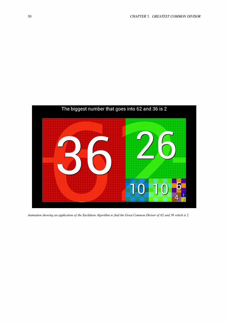
Animation showing an application of the Euclidean Algorithm to find the Great Common Divisor of 62 and 36 which is 2.

Chapter 6

Jordan’s totient function

Let k be a positive integer. In number theory, Jordan’s totient function Jk(n) of a positive integer n is the numberof k-tuples of positive integers all less than or equal to n that form a coprime (k + 1)-tuple together with n. This is ageneralisation of Euler’s totient function, which is J1. The function is named after Camille Jordan.

6.1 Definition

Jordan’s totient function is multiplicative and may be evaluated as

Jk(n) = nk∏p|n

(1− 1

pk

).

6.2 Properties•

∑d|n Jk(d) = nk.

which may be written in the language of Dirichlet convolutions as[1]

Jk(n) ⋆ 1 = nk

and via Möbius inversion as

Jk(n) = µ(n) ⋆ nk

Since the Dirichlet generating function of μ is 1/ζ(s) and the Dirichlet generating function of nk is ζ(s-k), the seriesfor J becomes

∑n≥1

Jk(n)

ns=ζ(s− k)

ζ(s)

• An average order of Jk(n) is

nk

ζ(k + 1)

• The Dedekind psi function is

31

32 CHAPTER 6. JORDAN’S TOTIENT FUNCTION

ψ(n) =J2(n)

J1(n)

and by inspection of the definition (recognizing that each factor in the product over the primes is a cyclotomic polyno-mial of p-k), the arithmetic functions defined by Jk(n)

J1(n)or J2k(n)

Jk(n)can also be shown to be integer-valued multiplicative

functions.

•∑

δ|n δsJr(δ)Js

(nδ

)= Jr+s(n) . [2]

6.3 Order of matrix groups

The general linear group of matrices of order m over Zn has order[3]

|GL(m,Zn)| = nm(m−1)

2

m∏k=1

Jk(n).

The special linear group of matrices of order m over Zn has order

| SL(m,Zn)| = nm(m−1)

2

m∏k=2

Jk(n).

The symplectic group of matrices of order m over Zn has order

| Sp(2m,Zn)| = nm2

m∏k=1

J2k(n).

The first two formulas were discovered by Jordan.

6.4 Examples

Explicit lists in the OEIS are J2 in A007434, J3 in A059376, J4 in A059377, J5 in A059378, J6 up to J10in A069091 up to A069095.

Multiplicative functions defined by ratios are J2(n)/J1(n) in A001615, J3(n)/J1(n) in A160889, J4(n)/J1(n) inA160891, J5(n)/J1(n) in A160893, J6(n)/J1(n) in A160895, J7(n)/J1(n) in A160897, J8(n)/J1(n) in

A160908, J9(n)/J1(n) in A160953, J10(n)/J1(n) in A160957, J11(n)/J1(n) in A160960.

Examples of the ratios J₂ (n)/J (n) are J4(n)/J2(n) in A065958, J6(n)/J3(n) in A065959, and J8(n)/J4(n) inA065960.

6.5 Notes

[1] Sándor & Crstici (2004) p.106

[2] Holden et al in external links The formula is Gegenbauer’s

[3] All of these formulas are from Andrici and Priticari in #External links

6.6. REFERENCES 33

6.6 References• L. E. Dickson (1971) [1919]. History of the Theory of Numbers, Vol. I. Chelsea Publishing. p. 147. ISBN0-8284-0086-5. JFM 47.0100.04.

• M. Ram Murty (2001). Problems in Analytic Number Theory. Graduate Texts in Mathematics 206. Springer-Verlag. p. 11. ISBN 0-387-95143-1. Zbl 0971.11001.

• Sándor, Jozsef; Crstici, Borislav (2004). Handbook of number theory II. Dordrecht: Kluwer Academic. pp.32–36. ISBN 1-4020-2546-7. Zbl 1079.11001.

6.7 External links• Andrica, Dorin; Piticari, Mihai (2004). “On some Extensions of Jordan’s arithmetical Functions”. Acta uni-versitatis Apulensis (7). MR 2157944.

• Holden, Matthew; Orrison, Michael; Varble, Michael. “Yet another Generalization of Euler’s Totient Func-tion”.

Chapter 7

Lehmer’s totient problem

For Lehmer’s Mahler measure problem, see Lehmer’s conjecture.

In mathematics, Lehmer’s totient problem, named for D. H. Lehmer, asks whether there is any composite numbern such that Euler’s totient function φ(n) divides n − 1. This is true of every prime number, and Lehmer conjecturedin 1932 that there are no composite solutions: he showed that if any such n exists, it must be odd, square-free, anddivisible by at least seven primes (i.e. ω(n) ≥ 7). Such a number must also be a Carmichael Number.

7.1 Properties

• In 1980 Cohen and Hagis proved that n > 1020 and that ω(n) ≥ 14.[1]

• In 1988 Hagis showed that if 3 divides n then n > 101937042 and ω(n) ≥ 298848.[2]

• The number of solutions to the problem less than X is O(X1/2(logX)3/4

).[3]

7.2 References

[1] Sándor et al (2006) p.23

[2] Guy (2004) p.142

[3] Sándor et al (2006) p.24

• Cohen, Graeme L.; Hagis, Peter, jun. (1980). “On the number of prime factors of n if φ(n) divides n−1”.Nieuw Arch. Wiskd., III. Ser. 28: 177–185. ISSN 0028-9825. Zbl 0436.10002.

• Guy, Richard K. (2004). Unsolved problems in number theory (3rd ed.). Springer-Verlag. B37. ISBN 0-387-20860-7. Zbl 1058.11001.

• Hagis, Peter, jun. (1988). “On the equation M⋅φ(n)=n−1”. Nieuw Arch. Wiskd., IV. Ser. 6 (3): 255–261.ISSN 0028-9825. Zbl 0668.10006.

• Lehmer, D. H. (1932). “On Euler’s totient function”. Bulletin of the American Mathematical Society 38: 745–751. doi:10.1090/s0002-9904-1932-05521-5. ISSN 0002-9904. Zbl 0005.34302.

• Ribenboim, Paulo (1996). The New Book of Prime Number Records (3rd ed.). New York: Springer-Verlag.ISBN 0-387-94457-5. Zbl 0856.11001.

• Sándor, József; Mitrinović, Dragoslav S.; Crstici, Borislav, eds. (2006). Handbook of number theory I. Dor-drecht: Springer-Verlag. ISBN 1-4020-4215-9. Zbl 1151.11300.

34

7.3. EXTERNAL LINKS 35

7.3 External links• Weisstein, Eric W., “Lehmer’s Totient Problem”, MathWorld.

Chapter 8

Liouville function

TheLiouville function, denoted by λ(n) and named after Joseph Liouville, is an important function in number theory.If n is a positive integer, then λ(n) is defined as:

λ(n) = (−1)Ω(n),

where Ω(n) is the number of prime factors of n, counted with multiplicity (sequence A008836 in OEIS).λ is completely multiplicative since Ω(n) is completely additive, i.e.: Ω(ab) = Ω(a) + Ω(b). The number one has noprime factors, so Ω(1) = 0 and therefore λ(1) = 1. The Liouville function satisfies the identity:

∑d|n

λ(d) =

1 ifnsquare, perfect a is0 otherwise.

The Liouville function’s Dirichlet inverse is the absolute value of the Möbius function.

8.1 Series

The Dirichlet series for the Liouville function is related to the Riemann zeta function by

ζ(2s)

ζ(s)=

∞∑n=1

λ(n)

ns.

The Lambert series for the Liouville function is

∞∑n=1

λ(n)qn

1− qn=

∞∑n=1

qn2

=1

2(ϑ3(q)− 1) ,

where ϑ3(q) is the Jacobi theta function.

8.2 Conjectures

The Pólya conjecture is a conjecture made by George Pólya in 1919. Defining

L(n) =n∑

k=1

λ(k),

36

8.3. REFERENCES 37

-140

-120

-100

-80

-60

-40

-20

0

0 1000 2000 3000 4000 5000 6000 7000 8000 9000 10000

sum

_k la

mbd

a(k)

n

Summatory Liouville function

Summatory Liouville function L(n) up to n = 104. The readily visible oscillations are due to the first non-trivial zero of the Riemannzeta function.

the conjecture states that L(n) ≤ 0 for n > 1. This turned out to be false. The smallest counter-example is n =906150257, found by Minoru Tanaka in 1980. It has since been shown that L(n) > 0.0618672√n for infinitely manypositive integers n,[1] while it can also be shown that L(n) < −1.3892783√n for infinitely many positive integers n.Define the related sum

T (n) =

n∑k=1

λ(k)

k.

It was open for some time whether T(n) ≥ 0 for sufficiently big n ≥ n0 (this “conjecture” is occasionally (but in-correctly) attributed to Pál Turán). This was then disproved by Haselgrove in 1958 (see the reference below), whoshowed that T(n) takes negative values infinitely often. A confirmation of this positivity conjecture would have ledto a proof of the Riemann hypothesis, as was shown by Pál Turán.

8.3 References[1] P. Borwein, R. Ferguson, and M. J. Mossinghoff, Sign Changes in Sums of the Liouville Function, Mathematics of Compu-

tation 77 (2008), no. 263, 1681–1694.

• Polya, G. (1919). “Verschiedene Bemerkungen zur Zahlentheorie”. Jahresbericht der DeutschenMathematiker-Vereinigung 28: 31–40.

• Haselgrove, C. B. (1958). “A disproof of a conjecture of Polya”. Mathematika 5 (2): 141–145. doi:10.1112/S0025579300001480.ISSN 0025-5793. MR 0104638. Zbl 0085.27102.

38 CHAPTER 8. LIOUVILLE FUNCTION

-3500

-3000

-2500

-2000

-1500

-1000

-500

0

0 1e+06 2e+06 3e+06 4e+06 5e+06 6e+06 7e+06 8e+06 9e+06 1e+07

sum

_k la

mbd

a(k)

n

Summatory Liouville function

Summatory Liouville function L(n) up to n = 107. Note the apparent scale invariance of the oscillations.

• Lehman, R. (1960). “On Liouville’s function”. Math. Comp. 14: 311–320. doi:10.1090/S0025-5718-1960-0120198-5. MR 0120198.

• Tanaka, Minoru (1980). “A Numerical Investigation on Cumulative Sum of the Liouville Function”. TokyoJournal of Mathematics 3 (1): 187–189. doi:10.3836/tjm/1270216093. MR 0584557.

• Weisstein, Eric W., “Liouville Function”, MathWorld.

• A.F. Lavrik (2001), “Liouville function”, in Hazewinkel, Michiel, Encyclopedia of Mathematics, Springer,ISBN 978-1-55608-010-4

8.3. REFERENCES 39

1

10

100

1000

10000

100000

1 10 100 1000 10000 100000 1e+06 1e+07 1e+08 1e+09 1e+10

sum

_k la

mbd

a(k)

n

Summatory Liouville function

Liouvillecounterexample

first zero

Logarithmic graph of the negative of the summatory Liouville function L(n) up to n = 2 × 109. The green spike shows the functionitself (not its negative) in the narrow region where the Pólya conjecture fails; the blue curve shows the oscillatory contribution of thefirst Riemann zero.

40 CHAPTER 8. LIOUVILLE FUNCTION

0

0.05

0.1

0.15

0.2

0.25

0.3

0 100 200 300 400 500 600 700 800 900 1000

sum

_k la

mbd

a(k)

/k

n

Liouville harmonic function

Harmonic Summatory Liouville functionM(n) up to n = 103

Chapter 9

Multiplicative function

Outside number theory, the term multiplicative function is usually used for completely multiplicativefunctions. This article discusses number theoretic multiplicative functions.

In number theory, amultiplicative function is an arithmetic function f(n) of the positive integer n with the propertythat f(1) = 1 and whenever a and b are coprime, then

f(ab) = f(a) f(b).

An arithmetic function f(n) is said to be completely multiplicative (or totally multiplicative) if f(1) = 1 and f(ab)= f(a) f(b) holds for all positive integers a and b, even when they are not coprime.

9.1 Examples

Some multiplicative functions are defined to make formulas easier to write:

• 1(n): the constant function, defined by 1(n) = 1 (completely multiplicative)

• 1C(n) the indicator function of the set C ⊂ Z . This is multiplicative if the set C has the property that if a andb are in C, gcd(a, b)=1, then ab is also in C. This is the case if C is the set of squares, cubes, or higher powers,or if C is the set of square-free numbers.

• Id(n): identity function, defined by Id(n) = n (completely multiplicative)

• Idk(n): the power functions, defined by Idk(n) = nk for any complex number k (completely multiplicative). Asspecial cases we have

• Id0(n) = 1(n) and• Id1(n) = Id(n).

• ϵ (n): the function defined by ϵ (n) = 1 if n = 1 and 0 otherwise, sometimes calledmultiplication unit for Dirichletconvolution or simply the unit function; the Kronecker delta δᵢn; sometimes written as u(n), not to be confusedwith µ (n) (completely multiplicative).

Other examples of multiplicative functions include many functions of importance in number theory, such as:

• gcd(n,k): the greatest common divisor of n and k, as a function of n, where k is a fixed integer.

• φ (n): Euler’s totient function φ , counting the positive integers coprime to (but not bigger than) n

41

42 CHAPTER 9. MULTIPLICATIVE FUNCTION

• µ (n): the Möbius function, the parity (−1 for odd, +1 for even) of the number of prime factors of square-freenumbers; 0 if n is not square-free

• σ k(n): the divisor function, which is the sum of the k-th powers of all the positive divisors of n (where k maybe any complex number). Special cases we have

• σ 0(n) = d(n) the number of positive divisors of n,• σ 1(n) = σ (n), the sum of all the positive divisors of n.

• a(n) : the number of non-isomorphic abelian groups of order n.

• λ (n): the Liouville function, λ(n) = (−1)Ω(n) where Ω(n) is the total number of primes (counted with multi-plicity) dividing n. (completely multiplicative).

• γ (n), defined by γ (n) = (−1) ω (n), where the additive function ω (n) is the number of distinct primes dividingn.

• All Dirichlet characters are completely multiplicative functions. For example

• (n/p), the Legendre symbol, considered as a function of n where p is a fixed prime number.

An example of a non-multiplicative function is the arithmetic function r2(n) - the number of representations of n asa sum of squares of two integers, positive, negative, or zero, where in counting the number of ways, reversal of orderis allowed. For example:

1 = 12 + 02 = (−1)2 + 02 = 02 + 12 = 02 + (−1)2

and therefore r2(1) = 4 ≠ 1. This shows that the function is not multiplicative. However, r2(n)/4 is multiplicative.In the On-Line Encyclopedia of Integer Sequences, sequences of values of a multiplicative function have the keyword“mult”.See arithmetic function for some other examples of non-multiplicative functions.

9.2 Properties

A multiplicative function is completely determined by its values at the powers of prime numbers, a consequence ofthe fundamental theorem of arithmetic. Thus, if n is a product of powers of distinct primes, say n = pa qb ..., thenf(n) = f(pa) f(qb) ...This property of multiplicative functions significantly reduces the need for computation, as in the following examplesfor n = 144 = 24 · 32:

d(144) = σ 0(144) = σ 0(24) σ 0(32) = (10 + 20 + 40 + 80 + 160)(10 + 30 + 90) = 5 · 3 = 15,σ (144) = σ 1(144) = σ 1(24) σ 1(32) = (11 + 21 + 41 + 81 + 161)(11 + 31 + 91) = 31 · 13 = 403,σ *(144) = σ *(24) σ *(32) = (11 + 161)(11 + 91) = 17 · 10 = 170.

Similarly, we have:

φ (144)= φ (24) φ (32) = 8 · 6 = 48

In general, if f(n) is a multiplicative function and a, b are any two positive integers, then

f(a) · f(b) = f(gcd(a,b)) · f(lcm(a,b)).

Every completely multiplicative function is a homomorphism of monoids and is completely determined by its restric-tion to the prime numbers.

9.3. CONVOLUTION 43

9.3 Convolution

If f and g are two multiplicative functions, one defines a new multiplicative function f * g, the Dirichlet convolutionof f and g, by

(f ∗ g)(n) =∑d|n

f(d) g(nd

)where the sum extends over all positive divisors d of n. With this operation, the set of all multiplicative functionsturns into an abelian group; the identity element is ϵ . Convolution is commutative, associative, and distributive overaddition.Relations among the multiplicative functions discussed above include:

• µ * 1 = ϵ (the Möbius inversion formula)

• ( µ Idk) * Idk = ϵ (generalized Möbius inversion)

• φ * 1 = Id

• d = 1 * 1

• σ = Id * 1 = φ * d

• σ k = Idk * 1

• Id = φ * 1 = σ * µ

• Idk = σ k * µ

The Dirichlet convolution can be defined for general arithmetic functions, and yields a ring structure, the Dirichletring.

9.3.1 Dirichlet series for some multiplicative functions

•∑

n≥1µ(n)ns = 1

ζ(s)

•∑

n≥1φ(n)ns = ζ(s−1)

ζ(s)

•∑

n≥1d(n)2

ns = ζ(s)4

ζ(2s)

•∑

n≥12ω(n)

ns = ζ(s)2

ζ(2s)

More examples are shown in the article on Dirichlet series.

9.4 Multiplicative function over F [X]

Let A=F [X], the polynomial ring over the finite field with q elements. A is principal ideal domain and therefore A isunique factorization domain.a complex-valued function λ on A is called multiplicative if λ(fg) = λ(f)λ(g) , whenever f and g are relativelyprime.

44 CHAPTER 9. MULTIPLICATIVE FUNCTION

9.4.1 Zeta function and Dirichlet series in F [X]

Let h be a polynomial arithmetic function (i.e. a function on set of monic polynomials over A). Its correspondingDirichlet series define to beDh(s) =

∑fmonic h(f)|f |−s ,

where for g ∈ A , set |g| = qdeg(g) if g = 0 , and |g| = 0 otherwise.The polynomial zeta function is thenζA(s) =

∑fmonic |f |−s .

Similar to the situation in N, every Dirichlet series of a multiplicative function h has a product representation (Eulerproduct):Dh(s) =

∏P (

∑∞n=0 h(P

n)|P |−sn) ,Where the product runs over all monic irreducible polynomials P.For example, the product representation of the zeta function is as for the integers: ζA(s) =

∏P (1− |P |−s)−1 .

Unlike the classical zeta function, ζA(s) is a simple rational function:ζA(s) =

∑f (|f |−s) =

∑n

∑deg(f)=n q

−sn =∑

n(qn−sn) = (1− q1−s)−1 .

In a similar way, If ƒ and g are two polynomial arithmetic functions, one defines ƒ * g, the Dirichlet convolution of ƒand g, by

(f ∗ g)(m) =∑d |m

f(m)g(md

)=

∑ab= f

f(a)g(b)

where the sum extends over all monic divisors d ofm, or equivalently over all pairs (a, b) of monic polynomials whoseproduct is m. The identity DhDg = Dh∗g still holds.

9.5 See also• Euler product

• Bell series

• Lambert series

9.6 References• See chapter 2 of Apostol, Tom M. (1976), Introduction to analytic number theory, Undergraduate Texts inMathematics, NewYork-Heidelberg: Springer-Verlag, ISBN978-0-387-90163-3,MR0434929, Zbl 0335.10001

9.7 External links• Planet Math

Chapter 10

Möbius function

This article is about the number-theoretic Möbius function. For the combinatorial Möbius function, see incidencealgebra.

For the rational functions defined on the complex numbers, see Möbius transformation.

The classicalMöbius function μ(n) is an important multiplicative function in number theory and combinatorics. TheGerman mathematician August Ferdinand Möbius introduced it in 1832.[1][2] It is a special case of a more generalobject in combinatorics.

10.1 Definition

For any positive integer n, define μ(n) as the sum of the primitive n-th roots of unity. It has values in −1, 0, 1depending on the factorization of n into prime factors:

• μ(n) = 1 if n is a square-free positive integer with an even number of prime factors.

• μ(n) = −1 if n is a square-free positive integer with an odd number of prime factors.

• μ(n) = 0 if n has a squared prime factor.

The values of μ(n) for the first 30 positive numbers (sequence A008683 in OEIS) areThe first 50 values of the function are plotted below:

The 50 first values of μ(n)

10.2 Properties and applications

45

46 CHAPTER 10. MÖBIUS FUNCTION

10.2.1 Properties

The Möbius function is multiplicative (i.e. μ(ab) = μ(a) μ(b) whenever a and b are coprime). The sum of the Möbiusfunction over all positive divisors of n (including n itself and 1) is zero except when n = 1:

∑d|n

µ(d) =

1 if n = 1

0 if n > 1.

This is because the n-th roots of unity sum to 0, and each n-th root of unity is a primitive d-th root of unity for exactlyone divisor d of n.The equality above leads to the important Möbius inversion formula and is the main reason why μ is of relevance inthe theory of multiplicative and arithmetic functions.Other applications of μ(n) in combinatorics are connected with the use of the Pólya enumeration theorem in combi-natorial groups and combinatorial enumerations.

10.2.2 Mertens function

In number theory another arithmetic function closely related to the Möbius function is the Mertens function, definedby

M(n) =n∑

k=1

µ(k)

for every natural number n. This function is closely linked with the positions of zeroes of the Riemann zeta function.See the article on the Mertens conjecture for more information about the connection betweenM(n) and the Riemannhypothesis.There is a formula[3] for calculating the Möbius function without directly knowing the factorization of its argument:

µ(n) =∑

1≤k≤n

gcd(k, n)=1

e2πikn ,

i.e. μ(n) is the sum of the primitive n-th roots of unity. (However, the computational complexity of this definition isat least the same as of the Euler Product definition.)From this it follows that the Mertens function is given by:

M(n) =∑a∈Fn

e2πia,

where Fn is the Farey sequence of order n.This formula is used in the proof of the Franel–Landau theorem.[4]

Proof of the formula for∑

d|n µ(d)

The formula given above,

∑d|n

µ(d) =

1 if n = 1

0 if n > 1.

10.2. PROPERTIES AND APPLICATIONS 47

is trivially true when n = 1. Suppose then that n > 1. Then there is a bijection between the factors d of n for whichμ(d) ≠ 0 and the subsets of the set of all prime factors of n. The asserted result follows from the fact that everynon-empty finite set has an equal number of odd- and even-cardinality subsets.This last fact can be shown easily by induction on the cardinality |S| of a non-empty finite set S. First, if |S| = 1,there is exactly one odd-cardinality subset of S, namely S itself, and exactly one even-cardinality subset, namely ∅.Next, if |S| > 1, then divide the subsets of S into two subclasses depending on whether they contain or not some fixedelement x in S. There is an obvious bijection between these two subclasses, pairing those subsets that have the samecomplement relative to the subset x. Also, one of these two subclasses consists of all the subsets of the set S \x,and therefore, by the induction hypothesis, has an equal number of odd- and even-cardinality subsets. These subsetsin turn correspond bijectively to the even- and odd-cardinality x-containing subsets of S. The inductive step followsdirectly from these two bijections.A related result is that the binomial coefficients exhibit alternating entries of odd and even power which sum sym-metrically.

10.2.3 Applications

Mathematical series

The Dirichlet series that generates the Möbius function is the (multiplicative) inverse of the Riemann zeta function;if s is a complex number with real part larger than 1 we have

∞∑n=1

µ(n)

ns=

1

ζ(s).

This may be seen from its Euler product

1

ζ(s)=

∏p∈P

(1− 1

ps

)=

(1− 1

2s

)(1− 1

3s

)(1− 1

5s

)· · · .

When s is a complex number with real part larger than 1, the Dirichlet series for the Möbius function also satisfies:

∞∑n=1

µ(n)

ns= 1−

∞∑a=2

1

as+

∞∑a=2

∞∑b=2

1

(a · b)s−

∞∑a=2

∞∑b=2

∞∑c=2

1

(a · b · c)s+

∞∑a=2

∞∑b=2

∞∑c=2

∞∑d=2

1

(a · b · c · d)s− · · · .

The Lambert series for the Möbius function is:

∑∞n=1

µ(n)qn

1−qn = q , which converges for |q| < 1.

The ordinary generating function for the Möbius function follows from the binomial series

(I +X)−1

applied to triangular matrices:

∞∑n=1

µ(n)xn = x−∞∑a=2

xa +∞∑a=2

∞∑b=2

xab −∞∑a=2

∞∑b=2

∞∑c=2

xabc +∞∑a=2

∞∑b=2

∞∑c=2

∞∑d=2

xabcd − · · ·

Algebraic number theory

Gauss[5] proved that for a prime number p the sum of its primitive roots is congruent to μ(p − 1) (mod p).

48 CHAPTER 10. MÖBIUS FUNCTION

If Fq denotes the finite field of order q (where q is necessarily a prime power), then the number N of monic irreduciblepolynomials of degree n over Fq is given by:[6]

N(q, n) =1

n

∑d|n

µ(d)qnd .

10.3 Recurrence

A simple recurrence for calculating the Möbius function without using the modulo function, is a combination of tworecurrences in a matrixM :

M(1, 1) = 1

n = k :M(n, k) = −i=k−1∑i=1

M(n, k − i)

n > k :M(n, k) =M(n− k, k)

n < k :M(n, k) = 0

This is a matrix starting:

M =

1 0 0 0 0 0 01 −1 0 0 0 0 01 0 −1 0 0 0 01 −1 0 0 0 0 01 0 0 0 −1 0 01 −1 −1 0 0 1 01 0 0 0 0 0 −1

10.4 Matrix inverse

The matrixM whereM(n, k) is equal to 1 if k divides n and equal to 0 otherwise:

M =

1 0 0 0 0 0 01 1 0 0 0 0 01 0 1 0 0 0 01 1 0 1 0 0 01 0 0 0 1 0 01 1 1 0 0 1 01 0 0 0 0 0 1

has the matrix inverse equal to µ(n/k) if k divides n and 0 otherwise:

M−1 =

1 0 0 0 0 0 0−1 1 0 0 0 0 0−1 0 1 0 0 0 00 −1 0 1 0 0 0−1 0 0 0 1 0 01 −1 −1 0 0 1 0−1 0 0 0 0 0 1

10.5. AVERAGE ORDER 49

10.5 Average order

The average order of theMöbius function is zero. This statement is, in fact, equivalent to the prime number theorem.[7]

10.6 μ(n) sections

μ(n) = 0 if and only if n is divisible by the square of a prime. The first numbers with this property are (sequenceA013929 in OEIS):

4, 8, 9, 12, 16, 18, 20, 24, 25, 27, 28, 32, 36, 40, 44, 45, 48, 49, 50, 52, 54, 56, 60, 63,....

If n is prime, then μ(n) = −1, but the converse is not true. The first non prime n for which μ(n) = −1 is 30 = 2·3·5.The first such numbers with three distinct prime factors (sphenic numbers) are:

30, 42, 66, 70, 78, 102, 105, 110, 114, 130, 138, 154, 165, 170, 174, 182, 186, 190, 195, 222, …(sequence A007304 in OEIS).

and the first such numbers with 5 distinct prime factors are:

2310, 2730, 3570, 3990, 4290, 4830, 5610, 6006, 6090, 6270, 6510, 6630, 7410, 7590, 7770, 7854,8610, 8778, 8970, 9030, 9282, 9570, 9690, … (sequence A046387 in OEIS).

10.7 Generalizations

10.7.1 Incidence algebras

In combinatorics, every locally finite partially ordered set (poset) is assigned an incidence algebra. One distinguishedmember of this algebra is that poset’s “Möbius function”. The classical Möbius function treated in this article isessentially equal to the Möbius function of the set of all positive integers partially ordered by divisibility. See thearticle on incidence algebras for the precise definition and several examples of these general Möbius functions.

10.7.2 Popovici’s function

Popovici defined a generalised Möbius function µk = µ⋆ · · ·⋆µ to be the k-fold Dirichlet convolution of the Möbiusfunction with itself. It is thus again a multiplicative function with

µk(pa) = (−1)a

(k

a

)where the binomial coefficient is taken to be zero if a > k. The definition may be extended to complex k by readingthe binomial as a polynomial in k.[8]

10.8 Physics

The Möbius function also arises in the primon gas or free Riemann gas model of supersymmetry. In this theory,the fundamental particles or “primons” have energies log p. Under second quantization, multiparticle excitations areconsidered; these are given by log n for any natural number n. This follows from the fact that the factorization of thenatural numbers into primes is unique.In the free Riemann gas, any natural number can occur, if the primons are taken as bosons. If they are taken asfermions, then the Pauli exclusion principle excludes squares. The operator (−1)F that distinguishes fermions andbosons is then none other than the Möbius function μ(n).

50 CHAPTER 10. MÖBIUS FUNCTION

The free Riemann gas has a number of other interesting connections to number theory, including the fact that thepartition function is the Riemann zeta function. This idea underlies Connes's attempted proof of the Riemann hy-pothesis.[9]

10.9 See also• Mertens function

• Liouville function

• Ramanujan’s sum

• Sphenic number

10.10 Notes[1] Hardy &Wright, Notes on ch. XVI: "... μ(n) occurs implicitly in the works of Euler as early as 1748, but Möbius, in 1832,

was the first to investigate its properties systematically.”

[2] In the Disquisitiones Arithmeticae (1801) Carl Friedrich Gauss showed that the sum of the primitive roots (mod p) is μ(p− 1), (see #Properties and applications) but he didn't make further use of the function. In particular, he didn't use Möbiusinversion in the Disquisitiones.

[3] Hardy & Wright 1980, (16.6.4), p. 239

[4] Edwards, Ch. 12.2

[5] Gauss, Disquisitiones, Art. 81

[6] Jacobson 2009, §4.13

[7] Apostol 1976, §3.9

[8] Sandor & Crstici (2004) p.107

[9] J.-B. Bost and Alain Connes (1995), “Hecke Algebras, Type III factors and phase transitions with spontaneous symmetrybreaking in number theory”, Selecta Math. (New Series), 1 411-457.

10.11 References

TheDisquisitiones Arithmeticae has been translated fromLatin into English andGerman. TheGerman edition includesall of his papers on number theory: all the proofs of quadratic reciprocity, the determination of the sign of the Gausssum, the investigations into biquadratic reciprocity, and unpublished notes.

• Gauss, Carl Friedrich (1986), Disquisitiones Arithemeticae, Arthur A. Clarke (English translator) (corrected2nd ed.), New York: Springer, ISBN 0-387-96254-9

• Gauss, Carl Friedrich (1965), Untersuchungen uber hohere Arithmetik (Disquisitiones Arithemeticae & otherpapers on number theory), H. Maser (German translator) (2nd ed.), New York: Chelsea, ISBN 0-8284-0191-8

• Apostol, Tom M. (1976), Introduction to analytic number theory, Undergraduate Texts in Mathematics, NewYork-Heidelberg: Springer-Verlag, ISBN 978-0-387-90163-3, MR 0434929, Zbl 0335.10001

• Computing the summation of theMöbius function byMarc Deléglise and Joël Rivat ExperimentalMathematicsVolume 5, Issue 4291-295

• Edwards, Harold (1974), Riemann’s Zeta Function, Mineola, New York: Dover, ISBN 0-486-41740-9

• Hardy, G. H.; Wright, E. M. (1980), An Introduction to the Theory of Numbers (5th ed.), Oxford: OxfordUniversity Press, ISBN 978-0-19-853171-5

10.12. EXTERNAL LINKS 51

• Jacobson, Nathan (2009) [1985], Basic algebra I (2nd ed.), Dover Publications, ISBN 978-0-486-47189-1

• Sándor, József; Mitrinović, Dragoslav S.; Crstici, Borislav, eds. (2006), Handbook of number theory I, Dor-drecht: Springer-Verlag, pp. 187–226, ISBN 1-4020-4215-9, Zbl 1151.11300

• Sándor, Jozsef; Crstici, Borislav (2004), Handbook of number theory II, Dordrecht: Kluwer Academic, ISBN1-4020-2546-7, Zbl 1079.11001

• N.I. Klimov (2001), “Möbius function”, in Hazewinkel, Michiel, Encyclopedia of Mathematics, Springer, ISBN978-1-55608-010-4

• Ed Pegg, Jr., "The Möbius function (and squarefree numbers)", MAA Online Math Games (2003)

10.12 External links• Weisstein, Eric W., “Möbius function”, MathWorld.

• http://ghmath.wordpress.com/2010/06/20/recursive-relation-for-the-mobius-function/

• http://terrytao.wordpress.com/2008/07/13/the-mobius-and-nilsequences-conjecture/

Chapter 11

Radical of an integer

In number theory, the radical of a positive integer n is defined as the product of the distinct prime numbers dividingn (each prime factor of n occurs exactly once as a factor of the product mentioned):

rad(n) =∏p|n

pprime

p

11.1 Examples

Radical numbers for the first few positive integers are

1, 2, 3, 2, 5, 6, 7, 2, 3, 10, ... (sequence A007947 in OEIS).

For example,

504 = 23 · 32 · 7

and therefore

rad(504) = 2 · 3 · 7 = 42

11.2 Properties

The function rad is multiplicative (but not completely multiplicative).The radical of any integer n is the largest square-free divisor of n and so also described as the square-free kernel ofn.[1] The definition is generalized to the largest t-free divisor of n, radt , which are multiplicative functions which acton prime powers as

radt(pe) = pmin(e,t−1)

The cases t=3 and t=4 are tabulated in A007948 and A058035.One of the most striking applications of the notion of radical occurs in the abc conjecture, which states that, for anyε > 0, there exists a finite Kε such that, for all triples of coprime positive integers a, b, and c satisfying a + b = c,

c < Kε rad(abc)1+ε

Furthermore, it can be shown that the nilpotent elements of Z/nZ are all of the multiples of rad(n).

52

11.3. SEE ALSO 53

11.3 See also• Radical of an ideal

11.4 References[1] (sequence A007947 in OEIS)

• Guy, Richard K. (2004). Unsolved Problems in Number Theory. Springer-Verlag. p. 102. ISBN 0-387-20860-7.

Chapter 12

Ramanujan tau function

The Ramanujan tau function, studied by Ramanujan (1916), is the function τ : N → Z defined by the followingidentity:

∑n≥1

τ(n)qn = q∏n≥1

(1− qn)24 = η(z)24 = ∆(z),

where q = exp(2πiz) with ℑz > 0 and η is the Dedekind eta function and the function∆(z) is a holomorphic cuspform of weight 12 and level 1, known as the discriminant modular form.

Values of |τ(n)| for n < 16,000 with logarithmic scale. The blue line picks only the values of n that are multiples of 121.

12.1 Values

The first few values of the tau function are given in the following table (sequence A000594 in OEIS):

54

12.2. RAMANUJAN’S CONJECTURES 55

12.2 Ramanujan’s conjectures

Ramanujan (1916) observed, but could not prove, the following three properties of τ(n) :

• τ(mn) = τ(m)τ(n) if gcd(m,n) = 1 (meaning that τ(n) is a multiplicative function)• τ(pr+1) = τ(p)τ(pr)− p11τ(pr−1) for p prime and r > 0.• |τ(p)| ≤ 2p11/2 for all primes p.

The first two properties were proved by Mordell (1917) and the third one, called the Ramanujan conjecture, wasproved by Deligne in 1974 as a consequence of his proof of the Weil conjectures.

12.3 Congruences for the tau function

For k ∈ Z and n ∈ Z>₀, define σk(n) as the sum of the k-th powers of the divisors of n. The tau function satisfiesseveral congruence relations; many of them can be expressed in terms of σk(n). Here are some:[1]

1. τ(n) ≡ σ11(n) mod 211 for n ≡ 1 mod 8 [2]

2. τ(n) ≡ 1217σ11(n) mod 213 for n ≡ 3 mod 8 [2]

3. τ(n) ≡ 1537σ11(n) mod 212 for n ≡ 5 mod 8 [2]

4. τ(n) ≡ 705σ11(n) mod 214 for n ≡ 7 mod 8 [2]

5. τ(n) ≡ n−610σ1231(n) mod 36 for n ≡ 1 mod 3 [3]

6. τ(n) ≡ n−610σ1231(n) mod 37 for n ≡ 2 mod 3 [3]

7. τ(n) ≡ n−30σ71(n) mod 53 for n ≡ 0 mod 5 [4]

8. τ(n) ≡ nσ9(n) mod 7 for n ≡ 0, 1, 2, 4 mod 7 [5]

9. τ(n) ≡ nσ9(n) mod 72 for n ≡ 3, 5, 6 mod 7 [5]

10. τ(n) ≡ σ11(n) mod 691. [6]

For p ≠ 23 prime, we have[1][7]

1. τ(p) ≡ 0 mod 23 if(

p23

)= −1

2. τ(p) ≡ σ11(p) mod 232 if p form the of is a2 + 23b2 [8]

3. τ(p) ≡ −1 mod 23otherwise .

12.4 Conjectures on τ(n)

Suppose that f is a weight k integer newform and the Fourier coefficients a(n) are integers. Consider the problem: Iff does not have complexmultiplication, prove that almost all primes p have the property that a(p) = 0modp . Indeed,most primes should have this property, and hence they are called ordinary. Despite the big advances by Deligne andSerre on Galois representations, which determine a(n)modp for n coprime to p , we do not have any clue as to howto compute a(p)modp . The only theorem in this regard is Elkies’ famous result for modular elliptic curves, whichindeed guarantees that there are infinitely many primes p for which a(p) = 0 , which in turn is obviously 0modp .We do not know any examples of non-CM f with weight> 2 for which a(p) = 0mod p for infinitely many primes p(although it should be true for almost all p ). We also do not know any examples where a(p) = 0mod p for infinitelymany p . Some people had begun to doubt whether a(p) = 0modp indeed for infinitely many p . As evidence, manyprovided Ramanujan’s τ(p) (case of weight 12 ). The largest known p for which τ(p) = 0modp is p = 7758337633. The only solutions to the equation τ(p) ≡ 0modp are p = 2, 3, 5, 7, 2411, and 7758337633 up to 1010 .[9]

Lehmer (1947) conjectured that τ(n) = 0 for all n , an assertion sometimes known as Lehmer’s conjecture. Lehmerverified the conjecture for n < 214928639999 (Apostol 1997, p. 22). The following table summarizes progress onfinding successively larger values of n for which this condition holds.

56 CHAPTER 12. RAMANUJAN TAU FUNCTION

12.5 Notes[1] Page 4 of Swinnerton-Dyer 1973

[2] Due to Kolberg 1962

[3] Due to Ashworth 1968

[4] Due to Lahivi

[5] Due to D. H. Lehmer

[6] Due to Ramanujan 1916

[7] Due to Wilton 1930

[8] Due to J.-P. Serre 1968, Section 4.5

[9] Due to N. Lygeros and O. Rozier 2010

12.6 References• Apostol, T. M. (1997), “Modular Functions and Dirichlet Series in Number Theory”, New York: Springer-Verlag 2nd ed.

• Ashworth, M. H. (1968), Congruence and identical properties of modular forms (D. Phil. Thesis, Oxford)

• Kolberg, O. (1962), “Congruences for Ramanujan’s function τ(n)", Arbok Univ. Bergen Mat.-Natur. Ser. (11),MR 0158873, Zbl 0168.29502

• Lehmer, D.H. (1947), “The vanishing of Ramanujan’s function τ(n)",DukeMath. J. 14: 429–433, doi:10.1215/s0012-7094-47-01436-1, Zbl 0029.34502

• Lygeros, N. (2010), “A New Solution to the Equation τ(p) ≡ 0 (mod p)" (PDF), Journal of Integer Sequences13: Article 10.7.4

• Mordell, Louis J. (1917), “On Mr. Ramanujan’s empirical expansions of modular functions.”, Proceedings ofthe Cambridge Philosophical Society 19: 117–124, JFM 46.0605.01

• Newman, M. (1972), “A table of τ (p) modulo p, p prime, 3 ≤ p ≤ 16067”, National Bureau of Standards.

• Rankin, Robert A. (1988), “Ramanujan’s tau-function and its generalizations”, inAndrews, George E.,Ramanujanrevisited (Urbana-Champaign, Ill., 1987), Boston, MA: Academic Press, pp. 245–268, ISBN 978-0-12-058560-1, MR 938968

• Ramanujan, Srinivasa (1916), “On certain arithmetical functions”, Trans. Cambridge Philos. Soc. 22 (9):159–184, MR 2280861

• Serre, J-P. (1968), “Une interprétation des congruences relatives à la fonction τ de Ramanujan”, SéminaireDelange-Pisot-Poitou 14

• Swinnerton-Dyer, H. P. F. (1973), “On ℓ-adic representations and congruences for coefficients of modularforms”, in Kuyk, Willem; Serre, Jean-Pierre, Modular functions of one variable, III, Lecture Notes in Mathe-matics 350, pp. 1–55, ISBN 978-3-540-06483-1, MR 0406931

• Wilton, J. R. (1930), “Congruence properties of Ramanujan’s function τ(n)", Proceedings of the London Math-ematical Society 31: 1–10, doi:10.1112/plms/s2-31.1.1

Chapter 13

Unit function

In number theory, the unit function is a completely multiplicative function on the positive integers defined as:

ε(n) =

1, if n = 1

0, if n = 1

It is called the unit function because it is the identity element for Dirichlet convolution.[1]

It may be described as the "indicator function of 1” within the set of positive integers. It is also written as u(n) (notto be confused with μ(n)).

13.1 See also• Möbius inversion formula

• Heaviside step function

• Kronecker delta

13.2 References[1] Estrada, Ricardo (1995), “Dirichlet convolution inverses and solution of integral equations”, Journal of Integral Equations

and Applications 7 (2): 159–166, doi:10.1216/jiea/1181075867, MR 1355233.

57

58 CHAPTER 13. UNIT FUNCTION

13.3 Text and image sources, contributors, and licenses

13.3.1 Text• Carmichael’s totient function conjecture Source: https://en.wikipedia.org/wiki/Carmichael’s_totient_function_conjecture?oldid=

661578935 Contributors: Michael Hardy, Mattp, Rjwilmsi, HenningThielemann, David Eppstein, La Pianista, UnCatBot, XLinkBot,Virginia-American, Draugluin14, Citation bot 1, Gamewizard71, Jesse V., Deltahedron, MunChanYoung, Neelabh deka andAnonymous:7

• Completelymultiplicative function Source: https://en.wikipedia.org/wiki/Completely_multiplicative_function?oldid=670980262Con-tributors: Michael Hardy, Dcoetzee, Giftlite, Rich Farmbrough, Mandarax, JoshuaZ,Myasuda, Vanish2, JackSchmidt, Virginia-American,PV=nRT, Yobot, Andy.melnikov, Duoduoduo, Brad7777, Enyokoyama and Anonymous: 4

• Dedekind psi function Source: https://en.wikipedia.org/wiki/Dedekind_psi_function?oldid=607144813Contributors: Gandalf61, Giftlite,GeneWard Smith, MuDavid, Crisófilax, Bluebot, JoshuaZ,Myasuda, DD2K, SieBot, Addbot, Yobot, Raulshc, R. J. Mathar, Makecat-bot,Citizentoad and Anonymous: 4

• Euler’s totient function Source: https://en.wikipedia.org/wiki/Euler’s_totient_function?oldid=673705683 Contributors: AxelBoldt,CYD,Mav, Uriyan, BryanDerksen, Zundark, Fnielsen, XJaM,Michael Hardy, TakuyaMurata, Looxix~enwiki, Den fjättrade ankan~enwiki,Charles Matthews, Dysprosia, Evgeni Sergeev, Sabbut, Robbot, Bhalperin, PBS, Romanm, MathMartin, Sverdrup, Henrygb, Hadal,JackofOz, William S., Astaines, Giftlite, Sj, Anton Mravcek, Pashute, Jorge Stolfi, Siroxo, DemonThing, Neilc, Gubbubu, Andyabides,Histrion, Creidieki, Fintor, PhotoBox, Rich Farmbrough, Guanabot, Mazi, Kooo, Gauge, El C, Crisófilax, Helopticor, Obradovic Goran,Tos~enwiki, ClementSeveillac, Ncik~enwiki, Sligocki, Burn, Ciphergoth2, Woodstone, Oleg Alexandrov, Linas, Will Orrick, MFH,Dedalus, Tokek, Leapfrog314, Mandarax, Graham87, Jclemens, Rjwilmsi, JVz, Stsmith, Salix alba, Bubba73, FlaBot, Eubot, Maxal,Glenn L, Chobot, YurikBot, Wavelength, ChrisBoyle, RussBot, Islamsalah, Rwalker, Bota47, Arthur Rubin, Evilbu, LeonardoRob0t,Pred, GrinBot~enwiki, Bo Jacoby, SmackBot, Reedy, KocjoBot~enwiki, Chris the speller, Bluebot, Kurykh, Nbarth, Nberger, DHN-bot~enwiki, Darth Panda, Mistamagic28, Henning Makholm, A5b, Vriullop, JoshuaZ, Minna Sora no Shita, Loadmaster, Denshade,CmaccompH89, Sammy cologne, Madmath789, Traviscj, Bruno321, CRGreathouse, Meithan, Jokes Free4Me, ShelfSkewed, Hen-ningThielemann, Myasuda, Zahlentheorie, WillowW, Headbomb, JAnDbot, Asmeurer, Magioladitis, Craw-daddy, David Eppstein, Es-chnett, Silverferret4, Toobaz, Tarotcards, Daniel5Ko, Policron, Phirazo, Anonymous Dissident, Math-kika~enwiki, Bbukh, PHilfinger,Dogah, VVVBot, Gerakibot, Cwkmail, Oxymoron83, OKBot, Nusumareta, Anchor Link Bot, Mygerardromance, JustinW Smith, Faran-nan, Nnemo, JP.Martin-Flatin, DragonBot, Bender2k14, Xodarap00, Rulerofutumno, Zss123456789, McDutchy, Banano03, DumZi-BoT, Katsushi, Nicolae Coman, Virginia-American, Vianello, MystBot, Addbot, Twaz, Wirkstoff, Yobot, Doctorhook, KamikazeBot,AnomieBOT, Goadeff, Gowr, Xqbot, Derek Whitten, Control.valve, RibotBOT, Raulshc, Hxd1011, FrescoBot, Lagelspeil, Sfabriz,Grinevitski, Motomuku, John85, Citation bot 1, 00Ragora00, Adlerbot, Rameshngbot, RedBot, Toolnut, Mjs1991, Antonsusi, Lotje, An-dreasBlobel, RjwilmsiBot, Matsgranvik, EmausBot, Kasper Meerts, Cal-linux, Wham Bam Rock II, Dodgez, Shishir332, Lazuran1911,D.Lazard, Fabian Hassler, Brandmeister, Maschen, Sapphorain, Wreardan, Anita5192, Vibhavp01, ClueBot NG, Quandle, Helpful PixieBot, J.Dong820, BG19bot, Bengski68, CitationCleanerBot, Darkgroup, Deltahedron, Will Jagy, Spectral sequence, ZX95, ইনাম, Math-mensch, Mark.mitchell61, K9re11, Piman2000, Vxanica, Yesenadam, GeoffreyT2000, Jaatex, CR100 and Anonymous: 185

• Greatest common divisor Source: https://en.wikipedia.org/wiki/Greatest_common_divisor?oldid=675914933 Contributors: AxelBoldt,Carey Evans, Bryan Derksen, Zundark, Tarquin, Taw, XJaM, Hannes Hirzel, Michael Hardy, Palnatoke, SGBailey, TakuyaMurata, PoorYorick, Nikai, Ideyal, Revolver, Charles Matthews, Dcoetzee, Bemoeial, Dysprosia, Jitse Niesen, Hyacinth, SirJective, JorgeGG, Fredrik,Henrygb, Jleedev, Tosha, Giftlite, Tom harrison, Herbee, Jason Quinn, Nayuki, Espetkov, Blankfaze, Azuredu, Karl Dickman, Mormegil,Guanabot, KneeLess, Paul August, Bender235, ESkog, EmilJ, Spoon!, Obradovic Goran, Haham hanuka, LutzL, Jumbuck, Silver hr,Arthena, Kenyon, Oleg Alexandrov, Linas, LOL, Ruud Koot, WadeSimMiser, Qwertyus, Josh Parris, Rjwilmsi, Staecker, Bryan H Bell,SLi, VKokielov, Ichudov, Glenn L, Salvatore Ingala, Chobot, Wavelength, Hyad, Dantheox, Planetscape, Werdna, Dan337, JCipriani,Arthur Rubin, Xnyper, Gesslein, Allens, Bo Jacoby, SmackBot, KnowledgeOfSelf, Pokipsy76, Gilliam, Janmarthedal, Kevin Ryde, Ar-mend, Ianmacm, Cybercobra, Decltype, Jiddisch~enwiki, Jbergquist, NeMewSys, Lambiam, Breno, Joaoferreira, Hu12, Shoeofdeath,Tauʻolunga, Philiprbrenan, Moreschi, Myasuda, Sopoforic, Wrwrwr, Sytelus, Casliber, Knakts, Marek69, TangentCube, Natalie Erin,AntiVandalBot, Nehuse~enwiki, Waerloeg, Salgueiro~enwiki, Normanzhang, JAnDbot, Turgidson, VoABot II, JamesBWatson, Ridhibookworm, Stdazi, David Eppstein, Vssun, Aconcagua, Patstuart, Genghiskhanviet, Captain panda, GeneralHooHa, Spnashville, Ind-watch, TomyDuby, Michael M Clarke, EyeRmonkey, Matiasholte, Gogobera, VolkovBot, DrMicro, JohnBlackburne, TXiKiBoT, Nx-avar, Aymatth2, Billinghurst, AlleborgoBot, Guno1618, Closenplay, Finnrind, AmigoNico, SieBot, Yintan, Anchor Link Bot, DixonD,Wabbit98, Startswithj, ClueBot, Vladkornea, Foxj, Mild Bill Hiccup, Bender2k14, Johnuniq, Crazy Boris with a red beard, Marc vanLeeuwen, Little Mountain 5, Mifter, Addbot, Mohammadrdeh~enwiki, Aboctok, Krslavin, Jarble, Luckas-bot, Yobot, Dav!dB, II Mus-LiM HyBRiD II, KamikazeBot, , Orion11M87, AnomieBOT, DemocraticLuntz, Citation bot, Geregen2, ArthurBot, Sniper 95jonas, Shirik, RibotBOT, Raulshc, FrescoBot, ComputScientist, Citation bot 1, MacMed, RedBot, Thelawoffives, FoxBot, Περίεργος,WikiTome, Shanefb, Ripchip Bot, DASHBot, John of Reading, Orphan Wiki, ZéroBot, AvicAWB, Quondum, D.Lazard, Aughost, Erolupin 3, Thine Antique Pen, HupHollandHup, Ipsign, Howard nyc, Tmvphil, Anita5192, ClueBot NG, Pesit, Cwinstanley, Mrjoerizkallah,Solomon7968, MC-CPO, BattyBot, Ves123, Webclient101, MindAfterMath, Lugia2453, PrunusDulcis, Fox2k11, Slurpy121, Haruhi-saito, Simdugas, Mathbees, DavidLeighEllis, Hollylilholly, Monkbot, Prof. Mc, Natarajpedia, Loraof, Pj.spaenlehauer and Anonymous:258

• Jordan’s totient function Source: https://en.wikipedia.org/wiki/Jordan’s_totient_function?oldid=631037534 Contributors: MichaelHardy, Jitse Niesen, Giftlite, RDBury, Vanish2, David Eppstein, Anonymous Dissident, Virginia-American, Addbot, Raulshc, FrescoBot,HRoestBot, R. J. Mathar, Cobaltcigs, Sapphorain, ChrisGualtieri, Deltahedron, K9re11 and Anonymous: 3

• Lehmer’s totient problem Source: https://en.wikipedia.org/wiki/Lehmer’s_totient_problem?oldid=640478556 Contributors: MichaelHardy, Rjwilmsi, Ironholds, Anne Bauval, MathsPoetry, RjwilmsiBot, Deltahedron, Spectral sequence and Anonymous: 2

• Liouville function Source: https://en.wikipedia.org/wiki/Liouville_function?oldid=664722123 Contributors: AxelBoldt, XJaM,MichaelHardy, Robbot, Robinh, Giftlite, Elroch, Paul August, Bender235, Eric Kvaalen, Burn, Oleg Alexandrov, Linas, Salvatore Ingala, Yurik-Bot, DYLANLENNON~enwiki, Arthur Rubin, Gutworth, JoshuaZ,Generalcp702,Myasuda, David Eppstein,WATARU,Gfis, VolkovBot,TXiKiBoT, Alexbot, MystBot, Addbot, Download, Hallomotocar, Luckas-bot, Yobot, Ptrf, Auclairde, FrescoBot, LucienBOT, Rapture-Bot, Tigris35711, Spectral sequence, The new math, 069952497a, Media watch, Tall human, DG-on-WP and Anonymous: 20

13.3. TEXT AND IMAGE SOURCES, CONTRIBUTORS, AND LICENSES 59

• Multiplicative function Source: https://en.wikipedia.org/wiki/Multiplicative_function?oldid=646903714 Contributors: AxelBoldt, Zun-dark, XJaM, PierreAbbat, Miguel~enwiki, Dominus, CharlesMatthews, Timwi, Dcoetzee, Dysprosia, Sabbut, .mau., AlexPlank, Henrygb,Hoot, Wikibot, Giftlite, Anton Mravcek, ChickenMerengo, Rich Farmbrough, Guanabot, Rajsekar, Burn, Linas, Graham87, Jshadias,Bubba73, Baccala@freesoft.org, MathNerd, Maksim-e~enwiki, Octahedron80, Mhym, Cícero, Jim.belk, CRGreathouse, HenningTh-ielemann, Zahlentheorie, RobHar, WinBot, JAnDbot, David Eppstein, Dogah, Arwest, PerryTachett, Smithpith, HairyFotr, Virginia-American, MystBot, Addbot, Ozob, PV=nRT, Yobot, Auclairde, Kirontanvir11, R. J. Mathar, Brad7777, Rockhand, Zvishem and Anony-mous: 27

• Möbius function Source: https://en.wikipedia.org/wiki/M%C3%B6bius_function?oldid=645263365Contributors: AxelBoldt, LC~enwiki,XJaM, Roadrunner, FvdP, Michael Hardy, Dominus, GTBacchus, Ahoerstemeier, Cimon Avaro, Schneelocke, Revolver, Frieda, Timwi,Dysprosia, Fibonacci, Sabbut, Robbot, Romanm, Hadal, Sushi~enwiki, Tobias Bergemann, Giftlite, Herbee, Jason Quinn, Eequor, JustAnother Dan, Pne, DemonThing, Rich Farmbrough, Guanabot, Rajsekar, Zaslav, Tos~enwiki, Jumbuck, ABCD, Gene Nygaard, CON-FIQ, Imaginatorium, Linas, Karam.Anthony.K, Jshadias, Wikix, Bubba73, Chobot, YurikBot, JWB, Baccala@freesoft.org, Leonar-doRob0t, Maksim-e~enwiki, Adam majewski, Jushi, Gutworth, Chlewbot, Richard L. Peterson, CRGreathouse, CBM, Myasuda, Rob-Har, JAnDbot, David Eppstein, Alu042, Yonidebot, DavidCBryant, VolkovBot, Pleasantville, Tomaxer, Lampica, AlleborgoBot, SieBot,ClueBot, Justin W Smith, JP.Martin-Flatin, Bender2k14, PixelBot, Qwfp, XLinkBot, Virginia-American, Addbot, Loupeter, HerculeBot,Yobot, AnomieBOT, Rubinbot, Point-set topologist, Raulshc, Latest Incarnation, Auclairde, Citation bot 1, Toolnut, Matsgranvik, Veg nw,Sapphorain, Helpful Pixie Bot, Deltahedron, Spectral sequence, The new math, Russell157, Magellan 1480, YvooovY and Anonymous:55

• Radical of an integer Source: https://en.wikipedia.org/wiki/Radical_of_an_integer?oldid=660539055 Contributors: Michael Hardy,Charles Matthews, Oleg Alexandrov, MFH, NeoUrfahraner, CalJW, Maxal, Redgolpe, LDH, CRGreathouse, Thijs!bot, Vanish2, DavidEppstein, IPonomarev, Gfis, Kraftlos, Tomaxer, Arcfrk, Dogah, Rumping, SilvonenBot, Addbot, Roentgenium111, Borisich, Luckas-bot,Maxis ftw, Raulshc, EmausBot, ZéroBot, R. J. Mathar, BG19bot, SectionFinale, Deltahedron, K9re11, Teddyktchan and Anonymous: 8

• Ramanujan tau function Source: https://en.wikipedia.org/wiki/Ramanujan_tau_function?oldid=654148779 Contributors: The Anome,Michael Hardy, Charles Matthews, Jitse Niesen, Tpbradbury, Giftlite, Profvk, Nabla, Rjwilmsi, R.e.b., Lenthe, MvH, Cydebot, Head-bomb, RobHar, CompositeFan, Tarotcards, MystBot, Addbot, Omnipaedista, Kpym, Citation bot 1, Johanbosman, Tsa1v, Citation-CleanerBot, Deltahedron, Enyokoyama, Alfred E. Neumann 1, Anrnusna, K9re11 and Anonymous: 19

• Unit function Source: https://en.wikipedia.org/wiki/Unit_function?oldid=635820495 Contributors: Michael Hardy, EmilJ, Oleg Alexan-drov, Bubba73, Spacepotato, Gaius Cornelius, Zer0fighta, Maksim-e~enwiki, Melchoir, CBM, Cydebot, David Eppstein, R'n'B, Hyun-seok.shin, Addbot, Yobot, NobelBot, Erik9bot, Mohehab, Qetuth and Anonymous: 4

13.3.2 Images• File:24x60.svg Source: https://upload.wikimedia.org/wikipedia/commons/7/74/24x60.svg License: CC0 Contributors: Own work Origi-nal artist: The original uploader was Michael Hardy at English Wikipedia

• File:Absolute_Tau_function_for_x_up_to_16,000_with_logarithmic_scale.JPG Source: https://upload.wikimedia.org/wikipedia/commons/3/36/Absolute_Tau_function_for_x_up_to_16%2C000_with_logarithmic_scale.JPG License: CC BY-SA 3.0 Contributors:Own work Original artist: Alfred E. Neumann 1

• File:EulerPhi.svg Source: https://upload.wikimedia.org/wikipedia/commons/9/9b/EulerPhi.svgLicense: GFDLContributors: OwnworkOriginal artist: Pietro Battiston (it:User:Toobaz)

• File:EulerPhi100.svg Source: https://upload.wikimedia.org/wikipedia/commons/f/f3/EulerPhi100.svgLicense: CC0Contributors: Ownwork Original artist: User:Sverdrup

• File:Least_common_multiple.svg Source: https://upload.wikimedia.org/wikipedia/commons/9/9d/Least_common_multiple.svgLicense:GFDL Contributors: en wiki Original artist: Morn

• File:Liouville-big.svg Source: https://upload.wikimedia.org/wikipedia/commons/d/d0/Liouville-big.svg License: CC-BY-SA-3.0 Con-tributors: w:File:Lioville-big.svg Original artist: User:Linas

• File:Liouville-harmonic.svg Source: https://upload.wikimedia.org/wikipedia/en/1/1a/Liouville-harmonic.svg License: Cc-by-sa-3.0Contributors: ? Original artist: ?

• File:Liouville-log.svg Source: https://upload.wikimedia.org/wikipedia/commons/4/42/Liouville-log.svg License: CC-BY-SA-3.0 Con-tributors: Original uploaded on en.wikipedia (transferred to commons by Hagman) Original artist: Created by Linas Vepstas en:User:Linas

• File:Liouville.svg Source: https://upload.wikimedia.org/wikipedia/commons/2/2d/Liouville.svg License: CC-BY-SA-3.0 Contributors:Created by Linas Vepstas User:Linas Original artist: User:Linas

• File:Moebius_mu.svg Source: https://upload.wikimedia.org/wikipedia/commons/c/c8/Moebius_mu.svg License: Public domain Con-tributors:

• MöbiusMu.PNG Original artist: MöbiusMu.PNG: User:Tos• File:Number_theory_symbol.svg Source: https://upload.wikimedia.org/wikipedia/commons/0/01/Number_theory_symbol.svgLicense:

CC BY-SA 2.5 Contributors: SVG conversion of Nts.png Original artist: , previous versions by and• File:OEISicon_light.svg Source: https://upload.wikimedia.org/wikipedia/commons/d/d8/OEISicon_light.svg License: Public domainContributors: Own work Original artist: Watchduck (a.k.a. Tilman Piesk)

• File:Question_book-new.svg Source: https://upload.wikimedia.org/wikipedia/en/9/99/Question_book-new.svg License: Cc-by-sa-3.0Contributors:Created from scratch in Adobe Illustrator. Based on Image:Question book.png created by User:Equazcion Original artist:Tkgd2007

• File:The_Great_Common_Divisor_of_62_and_36_is_2.ogv Source: https://upload.wikimedia.org/wikipedia/commons/5/5f/The_Great_Common_Divisor_of_62_and_36_is_2.ogv License: CC BY-SA 4.0 Contributors: Own work Original artist: philiprbrenan

60 CHAPTER 13. UNIT FUNCTION

13.3.3 Content license• Creative Commons Attribution-Share Alike 3.0