multivariate stochastic volatility models - singapore
TRANSCRIPT
Econometric Reviews, 25(2–3):361–384, 2006Copyright © Taylor & Francis Group, LLCISSN: 0747-4938 print/1532-4168 onlineDOI: 10.1080/07474930600713465
MULTIVARIATE STOCHASTIC VOLATILITY MODELS:BAYESIAN ESTIMATION AND MODEL COMPARISON
Jun Yu � School of Economics and Social Sciences, Singapore ManagementUniversity, Singapore
Renate Meyer � Department of Statistics, University of Auckland,Auckland, New Zealand
� In this paper we show that fully likelihood-based estimation and comparison of multivariatestochastic volatility (SV) models can be easily performed via a freely available Bayesian softwarecalled WinBUGS. Moreover, we introduce to the literature several new specifications that arenatural extensions to certain existing models, one of which allows for time-varying correlationcoefficients. Ideas are illustrated by fitting, to a bivariate time series data of weekly exchangerates, nine multivariate SV models, including the specifications with Granger causality involatility, time-varying correlations, heavy-tailed error distributions, additive factor structure,and multiplicative factor structure. Empirical results suggest that the best specifications are thosethat allow for time-varying correlation coefficients.
Keywords DIC; Factors; Granger causality in volatility; Heavy-tailed distributions; MCMC;Multivariate stochastic volatility; Time-varying correlations.
JEL Classification C11; C15; C30; G12.
1. INTRODUCTION
Univariate stochastic volatility (SV) models offer powerful alternativesto ARCH-type models in accounting for both the conditional and theunconditional properties of volatility. Superior performance of univariateSV models over ARCH-type models is documented in Danielsson (1994)and Kim et al. (1998) in terms of in-sample fitting, and in Yu (2002) interms of out-of-sample forecasting. As a result, the univariate SV modelhas been the subject of considerable attention in the literature; see, forexample, Shephard (2005) for a collection of relevant studies on this topic.
Received November 22, 2004; Accepted November 12, 2005Address correspondence to Jun Yu, School of Economics and Social Sciences, Singapore
Management University, 90 Stamford Road, Singapore 178903; E-mail: [email protected]
362 J. Yu and R. Meyer
There are both theoretical and empirical reasons that there is agreat need to study multivariate volatility models. On the one hand,much of financial decision making, such as portfolio optimization, assetallocation, risk management, and asset pricing, clearly needs to takecorrelations into account. On the other hand, it is well known that financialmarket volatilities move together over time across assets. As a result, themultivariate ARCH models (MARCH) have attracted a lot of attention inmodern finance theory and enjoyed voluminous empirical applications;see Bauwens et al. (2006) and McAleer (2005) for the literature review.Important contributions are Bollerslev et al. (1998), Diebold and Nerlove(1989), Bollerslev (1990), Engle et al. (1990), Engle and Kroner (1995),Braun et al. (1995), Engle (2002), Tse and Tusi (2002), among manyothers.
Compared to the MARCH literature, the literature on multivariate SVis much more limited (see McAleer, 2005, a partial review of the literature,and Asai et al., 2006, for a more detailed review), reflected by much fewerpublished papers on the topic to date (Aguilar and West, 2000; Chib et al.,2005; Danielsson, 1998; Harvey et al., 1994; Liesenfeld and Richard, 2003;Pitt and Shephard, 1999). Yet the multivariate SV models have certainstatistical attractions relative to the MARCH models (Harvey et al., 1994).We believe there are several reasons that the multivariate SV models havehad fewer empirical applications. Firstly, the multivariate SV models aremore difficult to estimate. Although estimation is already an issue forthe MARCH models, it is believed that estimation is more of an issuefor the multivariate SV models. This is because, apart from the inherentproblems of multivariate models, such as high dimensionality of theparameter space and the required positive semidefiniteness of covariancematrices, the likelihood function has no closed form for the multivariateSV model. Secondly, as a result of difficulties with parameter estimation,the computation of model comparison criteria becomes extensive anddemanding. Thirdly, compared to abundant alternative specifications inMARCH, only a handful of multivariate SV model specifications haveappeared in the literature. As a result, the existing multivariate SV modelsmay not be able to describe some important stylized features of the data.
A variety of estimation methods have been proposed to estimate theSV models. Less efficient methods include GMM (Andersen and Sorensen,1996; Melino and Turnbull, 1990), the quasi-maximum likelihood method(Harvey et al., 1994), and the method of the empirical characteristicfunction (Knight et al., 2002). Fully likelihood-based methods includethe simulated maximum likelihood method (SML) (Danielsson, 1994;Durham, 2005; Richard and Zhang, 2004; Sandmann and Koopman, 1998),the numerical maximum likelihood method (Fridman and Harris, 1998),and the Bayesian Markov chain Monte Carlo (MCMC) methods (Jacquieret al., 1994; Kim et al., 1998). Andersen et al. (1999) documented a finite
Multivariate Stochastic Volatility Models 363
sample comparison of various methods in Monte Carlo studies and foundthat MCMC is one of the most efficient estimation tools. Not surprisingly,MCMC is generally regarded in the literature as a benchmark for efficiency.Furthermore, as a by-product of parameter estimation, MCMC methodsprovide smoothed estimates of latent variables (Jacquier et al., 1994).This is because MCMC augments the parameter space by including latentvariables. Moreover, unlike most frequentist methods reviewed above whoseinference is based on asymptotic arguments, MCMC inference is based onthe exact posterior distribution of parameters and latent variables. Anotheradvantage of MCMC is that numerical optimization is not needed ingeneral. This advantage is of practical importance, especially when a modelhas many estimated parameters. As a result, MCMC has been extensivelyused to estimate univariate SV models in the literature.
Meyer and Yu (2000) illustrated the ease of implementing Bayesianestimation of univariate SV models based on purpose-built MCMC softwarecalled BUGS (Bayesian analysis using Gibbs sampler) developed bySpiegelhalter et al. (1996).1 Since then, BUGS has been employed toestimate univariate SV models in a number of studies (for example, Berget al., 2004; Lancaster, 2004; Meyer et al., 2003; Selçuk, 2004; Yu, 2005).Furthermore, Berg et al. (2004) showed that model selection of alternativeunivariate SV models is easily performed using the deviance informationcriterion (DIC), which is computed by BUGS. Arguably, univariate SVmodels can now be handled routinely in a straightforward fashion. Unlikeunivariate SV models, however, “multivariate stochastic volatility models stillpose significant computational challenges to applied researchers” (Chanet al., 2005).
One of the main purposes of the present paper is to show that fullylikelihood-based estimation and comparison of multivariate SV modelscan be easily performed via the WINDOWS version of BUGS (WinBUGS)(Spiegelhalter et al., 2003).2 The contribution of our paper is twofold.First, we extend the literature by offering several interesting extensions tothe existing specifications. In particular, we specify a model that allows forGranger causality in volatility and a model with time-varying correlations.Second, we extend Meyer and Yu (2000) and Berg et al. (2004) to themultivariate setting and show that both estimation and model comparisonfor multivariate SV models can also be handled in the same way as forthe univariate case. We then illustrate the implementation by estimatingand comparing nine alternative multivariate SV models in an empiricalstudy. To the best of our knowledge, a comparison of such a rich class of
1Note that BUGS is available free of charge from http://www.mrc-bsu.cam.ac.uk/bugs/welcome.shtml for a variety of operating systems such as UNIX, LINUX, and WINDOWS.
2We have become aware of a recent contribution to the literature by Jungbacker and Koopman(2006), where a simulated maximum likelihood method is used to estimate three alternativemultivariate SV models.
364 J. Yu and R. Meyer
multivariate SV models has not been done before. The comparison resultsin several interesting empirical findings.
The remainder of the paper is organized as follows. In Section 2, weillustrate the differences among the existing multivariate SV models in abivariate setting and propose several new multivariate SV specifications.Section 3 reviews a Bayesian approach for parameter estimation usingWinBUGS. Section 4 briefly describes a Bayesian approach for modelcomparison via DIC. In Section 5, we illustrate the estimation andmodel comparison using an example of Australian/US dollar andNew Zealand/US dollar exchange rates. Section 6 concludes.
2. MULTIVARIATE SV MODELS
2.1. Stylized Facts of Financial Asset Returns
Considering that multivariate SV models are most useful for describingthe dynamics of financial asset returns, we first summarize some well-documented stylized facts of financial asset returns:
1. Asset return distributions are leptokurtic.2. Asset return volatilities cluster.3. Returns are cross-dependent.4. Volatilities are cross-dependent.5. Sometimes volatility of one asset Granger causes volatility of another
asset (that is, volatility spills over from one market to another market).6. There often exists a lower dimensional factor structure that can explain
most of the correlation.7. Correlations are time varying.
In addition to these seven stylized facts, the issues such as thedimensionality of the parameter space and positive semi-definiteness ofthe covariance matrix are of practical importance. When we review theexisting models and introduce our new models we will comment on theirappropriateness for dealing with the stylized facts and the two issues posedabove.
2.2. Alternative Specifications in a Bivariate Setting
To illustrate the difference and linkage among alternative multivariateSV models, we focus on the bivariate case in this paper. In particular,we consider nine different bivariate SV models (with acronyms in boldface), two of which are new to the literature. Moreover, most of thesespecifications are amenable to a multidimensional generalization, withModel 5 being the only exception.
Multivariate Stochastic Volatility Models 365
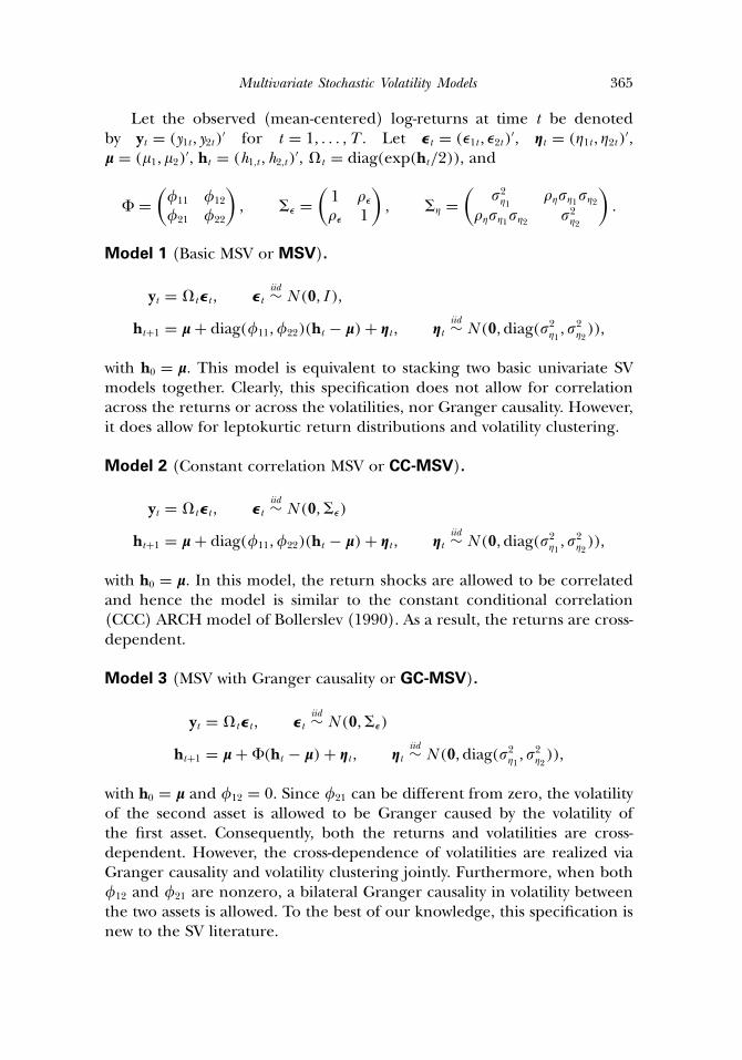
Let the observed (mean-centered) log-returns at time t be denotedby yt = (y1t , y2t)′ for t = 1, � � � ,T . Let �t = (�1t , �2t)′, �t = (�1t , �2t)′,� = (�1, �2)
′, ht = (h1,t , h2,t)′, �t = diag(exp(ht/2)), and
� =(�11 �12
�21 �22
), �� =
(1 �
� 1
), �� =
(2�1
��1�2
��1�2 2�2
)�
Model 1 (Basic MSV or MSV).
yt = �t�t , �tiid∼ N (0, I ),
ht+1 = � + diag(�11,�22)(ht − �) + �t , �tiid∼ N (0, diag(2
�1, 2
�2)),
with h0 = �. This model is equivalent to stacking two basic univariate SVmodels together. Clearly, this specification does not allow for correlationacross the returns or across the volatilities, nor Granger causality. However,it does allow for leptokurtic return distributions and volatility clustering.
Model 2 (Constant correlation MSV or CC-MSV).
yt = �t�t , �tiid∼ N (0,��)
ht+1 = � + diag(�11,�22)(ht − �) + �t , �tiid∼ N (0, diag(2
�1, 2
�2)),
with h0 = �. In this model, the return shocks are allowed to be correlatedand hence the model is similar to the constant conditional correlation(CCC) ARCH model of Bollerslev (1990). As a result, the returns are cross-dependent.
Model 3 (MSV with Granger causality or GC-MSV).
yt = �t�t , �tiid∼ N (0,��)
ht+1 = � + �(ht − �) + �t , �tiid∼ N (0, diag(2
�1, 2
�2)),
with h0 = � and �12 = 0. Since �21 can be different from zero, the volatilityof the second asset is allowed to be Granger caused by the volatility ofthe first asset. Consequently, both the returns and volatilities are cross-dependent. However, the cross-dependence of volatilities are realized viaGranger causality and volatility clustering jointly. Furthermore, when both�12 and �21 are nonzero, a bilateral Granger causality in volatility betweenthe two assets is allowed. To the best of our knowledge, this specification isnew to the SV literature.
366 J. Yu and R. Meyer
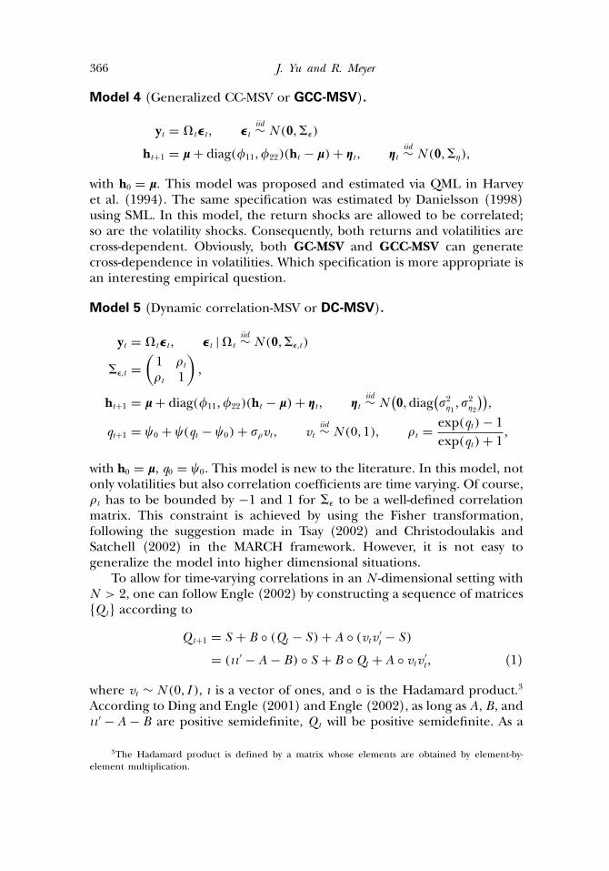
Model 4 (Generalized CC-MSV or GCC-MSV).
yt = �t�t , �tiid∼ N (0,��)
ht+1 = � + diag(�11,�22)(ht − �) + �t , �tiid∼ N (0,��),
with h0 = �. This model was proposed and estimated via QML in Harveyet al. (1994). The same specification was estimated by Danielsson (1998)using SML. In this model, the return shocks are allowed to be correlated;so are the volatility shocks. Consequently, both returns and volatilities arecross-dependent. Obviously, both GC-MSV and GCC-MSV can generatecross-dependence in volatilities. Which specification is more appropriate isan interesting empirical question.
Model 5 (Dynamic correlation-MSV or DC-MSV).
yt = �t�t , �t |�tiid∼ N (0,��,t)
��,t =(1 t
t 1
),
ht+1 = � + diag(�11,�22)(ht − �) + �t , �tiid∼ N
(0, diag
(2�1, 2
�2
)),
qt+1 = �0 + �(qt − �0) + vt , vtiid∼ N (0, 1), t = exp(qt) − 1
exp(qt) + 1,
with h0 = �, q0 = �0. This model is new to the literature. In this model, notonly volatilities but also correlation coefficients are time varying. Of course,t has to be bounded by −1 and 1 for �� to be a well-defined correlationmatrix. This constraint is achieved by using the Fisher transformation,following the suggestion made in Tsay (2002) and Christodoulakis andSatchell (2002) in the MARCH framework. However, it is not easy togeneralize the model into higher dimensional situations.
To allow for time-varying correlations in an N -dimensional setting withN > 2, one can follow Engle (2002) by constructing a sequence of matrices�Qt according to
Qt+1 = S + B ◦ (Qt − S) + A ◦ (vtv ′t − S)
= (��′ − A − B) ◦ S + B ◦ Qt + A ◦ vtv ′t , (1)
where vt ∼ N (0, I ), � is a vector of ones, and ◦ is the Hadamard product.3
According to Ding and Engle (2001) and Engle (2002), as long as A, B, and��′ − A − B are positive semidefinite, Qt will be positive semidefinite. As a
3The Hadamard product is defined by a matrix whose elements are obtained by element-by-element multiplication.
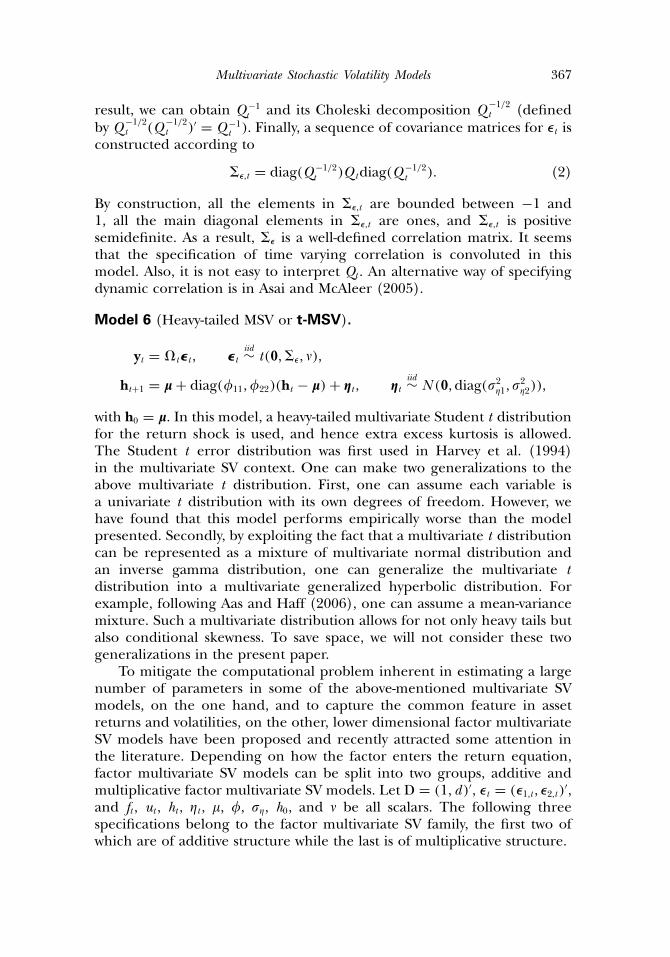
Multivariate Stochastic Volatility Models 367
result, we can obtain Q −1t and its Choleski decomposition Q −1/2
t (definedby Q −1/2
t (Q −1/2t )′ = Q −1
t ). Finally, a sequence of covariance matrices for �t isconstructed according to
��,t = diag(Q −1/2t )Qtdiag(Q −1/2
t )� (2)
By construction, all the elements in ��,t are bounded between −1 and1, all the main diagonal elements in ��,t are ones, and ��,t is positivesemidefinite. As a result, �� is a well-defined correlation matrix. It seemsthat the specification of time varying correlation is convoluted in thismodel. Also, it is not easy to interpret Qt . An alternative way of specifyingdynamic correlation is in Asai and McAleer (2005).
Model 6 (Heavy-tailed MSV or t-MSV).
yt = �t�t , �tiid∼ t(0,��, �),
ht+1 = � + diag(�11,�22)(ht − �) + �t , �tiid∼ N (0, diag(2
�1, 2�2)),
with h0 = �. In this model, a heavy-tailed multivariate Student t distributionfor the return shock is used, and hence extra excess kurtosis is allowed.The Student t error distribution was first used in Harvey et al. (1994)in the multivariate SV context. One can make two generalizations to theabove multivariate t distribution. First, one can assume each variable isa univariate t distribution with its own degrees of freedom. However, wehave found that this model performs empirically worse than the modelpresented. Secondly, by exploiting the fact that a multivariate t distributioncan be represented as a mixture of multivariate normal distribution andan inverse gamma distribution, one can generalize the multivariate tdistribution into a multivariate generalized hyperbolic distribution. Forexample, following Aas and Haff (2006), one can assume a mean-variancemixture. Such a multivariate distribution allows for not only heavy tails butalso conditional skewness. To save space, we will not consider these twogeneralizations in the present paper.
To mitigate the computational problem inherent in estimating a largenumber of parameters in some of the above-mentioned multivariate SVmodels, on the one hand, and to capture the common feature in assetreturns and volatilities, on the other, lower dimensional factor multivariateSV models have been proposed and recently attracted some attention inthe literature. Depending on how the factor enters the return equation,factor multivariate SV models can be split into two groups, additive andmultiplicative factor multivariate SV models. Let D = (1, d)′, �t = (�1,t , �2,t)′,and ft , ut , ht , �t , �, �, �, h0, and � be all scalars. The following threespecifications belong to the factor multivariate SV family, the first two ofwhich are of additive structure while the last is of multiplicative structure.
368 J. Yu and R. Meyer
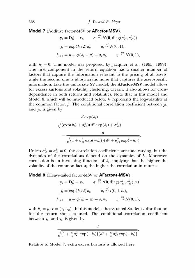
Model 7 (Additive factor-MSV or AFactor-MSV).
yt = Dft + �t , �tiid∼ N (0, diag(2
�1, 2�2))
ft = exp(ht/2)ut , utiid∼ N (0, 1),
ht+1 = � + �(ht − �) + ��t , �tiid∼ N (0, 1),
with h0 = 0. This model was proposed by Jacquier et al. (1995, 1999).The first component in the return equation has a smaller number offactors that capture the information relevant to the pricing of all assets,while the second one is idiosyncratic noise that captures the asset-specificinformation. Like the univariate SV model, the AFactor-MSV model allowsfor excess kurtosis and volatility clustering. Clearly, it also allows for cross-dependence in both returns and volatilities. Note that in this model andModel 8, which will be introduced below, ht represents the log-volatility ofthe common factor, ft . The conditional correlation coefficient between y1tand y2t is given by
d exp(ht)√(exp(ht) + 2
�1)(d2 exp(ht) + 2�2)
= d√(1 + 2
�1 exp(−ht))(d2 + 2�2 exp(−ht))
�
Unless 2�1 = 2
�2 = 0, the correlation coefficients are time varying, but thedynamics of the correlations depend on the dynamics of ht . Moreover,correlation is an increasing function of ht , implying that the higher thevolatility of the common factor, the higher the correlation in returns.
Model 8 (Heavy-tailed factor-MSV or AFactor-t-MSV).
yt = Dft + �t , �tiid∼ t(0, diag(2
�1, 2�2), �)
ft = exp(ht/2)ut , utiid∼ t(0, 1,�),
ht+1 = � + �(ht − �) + ��t , �tiid∼ N (0, 1),
with h0 = �, � = (�1, �2)′. In this model, a heavy-tailed Student t distributionfor the return shock is used. The conditional correlation coefficientbetween y1t and y2t is given by
d√(1 + �
�12�1 exp(−ht)
)(d2 + �
�22�2 exp(−ht)
) �
Relative to Model 7, extra excess kurtosis is allowed here.
Multivariate Stochastic Volatility Models 369
Model 9 (Multiplicative factor-MSV or MFactor-MSV).
yt = exp(ht/2)�t , �tiid∼ N (0,��),
ht+1 = � + �(ht − �) + ��t , �tiid∼ N (0, 1),
�� =(
1 ��2
��2 2�2
),
with h0 = �. This model, also known as the stochastic discount factormodel, was considered in Quintana and West (1987). Compared withModel 1 (MSV), this model has even fewer parameters. Obviously, it retainsall the properties inherent in the univariate SV model, such as excesskurtosis and volatility clustering. Cross-dependence in returns is inducedby the dependence in �t , but the correlations are time invariant. Moreover,the correlation in log-volatilities is always one, but time-varying correlationin returns is not allowed.
Most of the models reviewed above are nonnested with each other. Forexample, Model 9 (MFactor-MSV) is not nested with Model 7 (AFactor-MSV) or Model 8 (AFactor-t-MSV). Neither Model 7 nor Model 8 is nestedor nested within any other models, including Model 5 (DC-MSV). However,Model 9 (MFactor-MSV) can be viewed as a special case of Model 2 (CC-MSV), in which �1 = �2, �11 = �22, �1 = �2, �1t = �2t , and hence h1,t = h2,t .
3. BAYESIAN ESTIMATION USING WinBUGS
The models in Section 2.2 are completed by the specification of a priordistribution for all unknown parameters a = (a1, � � � , ap). For instance, inModel 1 (MSV), p = 6 and the vector a of unknown parameters is a =(�1, �2,�11,�22, 2
�1, 2�2). Bayesian inference is based on the joint posterior
distribution of all unobserved quantities � in the model. The vector �comprises the unknown parameters and the vector of latent log-volatilities,i.e., � = (a,h1, � � � ,hT ).
In the sequel, let p(·) denote the generic probability density functionof a random variable. Using independent priors for the parameters andsuccessive conditioning on the sequence of latent states, the joint priordensity of � in Model 1 is given by
p(a)p(h0)
T∏t=1
p(ht |a)
= p(�1)p(�2)p(�11)p(�22)p(2�1)p(
2�2)p(h0)
T∏t=1
p(ht |a)�
370 J. Yu and R. Meyer
After observing the data, this joint prior density is updated to thejoint posterior density of all unknown quantities, p(� | y) (where y =(y1, � � � , yT )) via Bayes’ theorem by multiplying prior p(�) and likelihoodp(y | �):
p(� | y) ∝ p(�)p(y | �) ∝ p(a)p(h0)
T∏t=1
p(ht |a)T∏t=1
p(yt |ht)� (3)
To calculate the marginal posterior distribution of the parametersof interest, p(a | y) requires (p + 2T )-dimensional integration to findthe normalization constant p(�)p(y | �)d� followed by 2T -dimensionalintegration over all latent volatilities, as
p(a | y) =∫h1
· · ·∫hT
p(a,h1, � � � ,hT )dhT · · · dh1� (4)
This is neither analytically nor numerically tractable in general. Simulation-based integration techniques have proven to be the most effectivemethods to deal with this integration problem. Say, a sample of size M ,(a(1),h(1), � � � ,a(M ),h(M )) can be obtained from p(� | y). By simply ignoringthe sampled latent volatilities, the subvector (a(1),a(2), � � � ,a(M )) constitutesa sample from the marginal posterior distribution (4) of a, and kerneldensity estimates of each component can be used to estimate the marginalposterior density of each parameter. The usual summary statistics can becalculated to estimate population quantities of interest, e.g., the samplemean 1
M
∑Mm=1 a
(m) is a consistent estimate of the posterior mean E [a | y].Unfortunately, direct independent sampling from a high-dimensional
distribution such as in (3) is usually not possible (see Liesenfeld andRichard, 2003 and Durham, 2005 for counterexamples, however). MCMCtechniques overcome this problem by constructing a Markov chain withstationary distribution equal to the target density p(� | y) and simulatefrom this Markov chain. Provided the Markov chain is run long enough tohave reached equilibrium, the samples in each iteration can be regardedas (dependent) samples from p(� | y). By the ergodic theorem, sampleaverages are still consistent estimates of the population quantities.
Care needs to be taken in determining the number of iterations toachieve convergence to the stationary distribution. Various convergencediagnostics have been developed and implemented in the CODA package,a collections of SPLUS or R routines. CODA may also be downloaded fromthe BUGS website.
Here, we advocate the software package WinBUGS for posteriorcomputation in multivariate SV models. WinBUGS provides an easy andefficient implementation of the Gibbs sampler, a specific MCMC techniquethat constructs a Markov chain by sampling from all univariate full
Multivariate Stochastic Volatility Models 371
conditional distributions in a cyclic way. WinBUGS has been successfullyapplied for a variety of statistical models such as random effects,generalized linear, proportional hazards, latent variable, and frailty models.In particular, state space models (Harvey, 1990), either linear or nonlinear,either Gaussian or non-Guassian, either observed state or latent state,either univariate or multivariate, are amenable to a Bayesian analysis viaWinBUGS.
Meyer and Yu (2000) described the use of BUGS for Bayesianposterior computation in univariate SV models and emphasized the easewith which BUGS can be used for the exploratory phase of modelbuilding, as any modifications of a model, including changes of priors andsampling error distributions, are readily realized with only minor changesof the code. BUGS automates the calculation of the full conditionalposterior distributions that are needed for Gibbs sampling using a modelrepresentation by directed acyclic graphs. It contains an expert systemfor choosing an effective sampling method for each full conditional.The reader is referred to Meyer and Yu (2000) for a comprehensiveintroduction on using BUGS for fitting SV models. WinBUGS is a newinteractive version of the BUGS program that allows models to bedescribed using a slightly amended version of the BUGS language. TheBUGS website contains a short Flash illustration on the basic steps ofrunning WinBUGS. WinBUGs also allows models to be fitted using Doodles(graphical representations of models by directed acyclic graphs), whichcan, if desired, be automatically translated into a text-based description.In Meyer and Yu (2000), the Doodle corresponding to a certain BUGSimplementation of a univariate SV model is explained in detail.
BUGS can be slow owing to the single-move Gibbs sampler. However,the new interactive WinBUGS version contains much-improved algorithmsto sample from the full conditional posterior distributions. WinBUGScontains a small expert system for choosing the best sampling method. Fordiscrete full conditional distributions, WinBUGS uses the inversion methodto simulate values. For continuous distributions, it tests first for conjugacy.If it detects conjugacy, then it will use optimized standard simulationalgorithms. For logconcave full conditionals, it uses the derivative-freeadaptive rejection technique of Gilks (1992). For nonlogconcave fullconditionals with restricted range, WinBUGS uses the slice samplingtechnique of Neal (1997) with an adaptive phase of 500 iterations anda current point Metropolis algorithm for unrestricted nonlogconcavefull conditionals. The current point Metropolis algorithm is based ona symmetric normal proposal distribution whose standard deviation istuned over the first 4,000 iterations in order to get an acceptance ratebetween 20% and 40%. Furthermore, it contains the option of usingordered overrelaxation (Neal, 1998) which generates multiple samplesat each iteration and then selects one that is negatively correlated with
372 J. Yu and R. Meyer
the current value. The time per iteration will be increased, but the within-chain correlations should be reduced, and hence fewer iterations may benecessary. It also contains a blocking option for multivariate updating,but only for generalized linear model components at this stage. Theuse of these improved sampling techniques coupled with an increase incomputational speed due to advances in computer hardware has made itpossible to fit multivariate SV models in WinBUGS.
4. DIC
The Akaike information criterion (AIC; Akaike, 1973) is a popularmethod for comparing alternative and possibly nonnested models. It tradesoff a measure of model adequacy, measured by the log-likelihood, againsta measure of complexity, measured by the number of free parameters.Obviously, the calculation of AIC requires the specification of the numberof free parameters. For a nonhierarchical Bayesian model with parameter�, obtaining the number of free parameters is straightforward. However,for a complex hierarchical model, the specification of the dimensionalityof the parameter space is rather arbitrary. This is typically the case for SVmodels. The reason is that when MCMC is used to estimate SV models, asmentioned above, the parameter space is augmented. For example, in thebasic MSV model, we include the 2T latent volatilities into the parameterspace with T being the sample size. As these volatilities are dependent, theycannot be counted as 2T additional free parameters. Consequently, AIC isnot applicable for comparing SV models (Berg et al., 2004).
The deviance information criterion (DIC) of Spiegelhalter et al. (2002)is intended as a generalization of AIC to complex hierarchical models. LikeAIC, DIC consists of two components,
DIC = D + pD , (5)
where the first term measures goodness of fit and the second term is apenalty term for increasing model complexity.
Spiegelhalter et al. (2002) give an asymptotic justification of DIC inthe case where the number of observations T grows with respect to thenumber of parameters p and where the prior is nonhierarchical andcompletely specified (i.e., without hyperparameters). Like AIC, the modelwith the smallest DIC is estimated to be the one that would best predicta replicate dataset of the same structure as that observed. This focusof DIC, however, is different from the posterior-odd-based approaches,where how well the prior has predicted the observed data is addressed.Berg et al. (2004) examined the performance of DIC relative to twoposterior odd approaches—one is based on the harmonic mean estimateof marginal likelihood (Newton and Raftery, 1994) and the other is Chib’s
Multivariate Stochastic Volatility Models 373
estimate of marginal likelihood (Chib, 1995)—in the context of univariateSV models. They found reasonably consistent performance of these threemodel comparison methods.
From the definition of DIC it can be seen that DIC is almosttrivial to compute and particularly suited to compare Bayesian modelswhen posterior distributions have been obtained using MCMC simulation.Indeed, DIC is automatically computed by WinBUGS1.4. This is incontrast to Chib’s marginal likelihood method, where computational costis more demanding as the likelihood needs to be evaluated using otherindependent procedures such as the particle filter (Kim et al., 1998).Although Chib et al. (2005) successfully used Chib’s method to compareseveral specifications in a family of factor multivariate SV with the additivestructure, we believe the computational tractability of DIC would make itfeasible to compare a much larger class of specifications.
It should be pointed out that because WinBUGS calculates DIC at theposterior mean, it requires the posterior mean to be a good estimate ofthe stochastic parameters. Therefore it is important to check skewness andmodality of the posterior distribution when using DIC.
5. EMPIRICAL ILLUSTRATION
5.1. Data
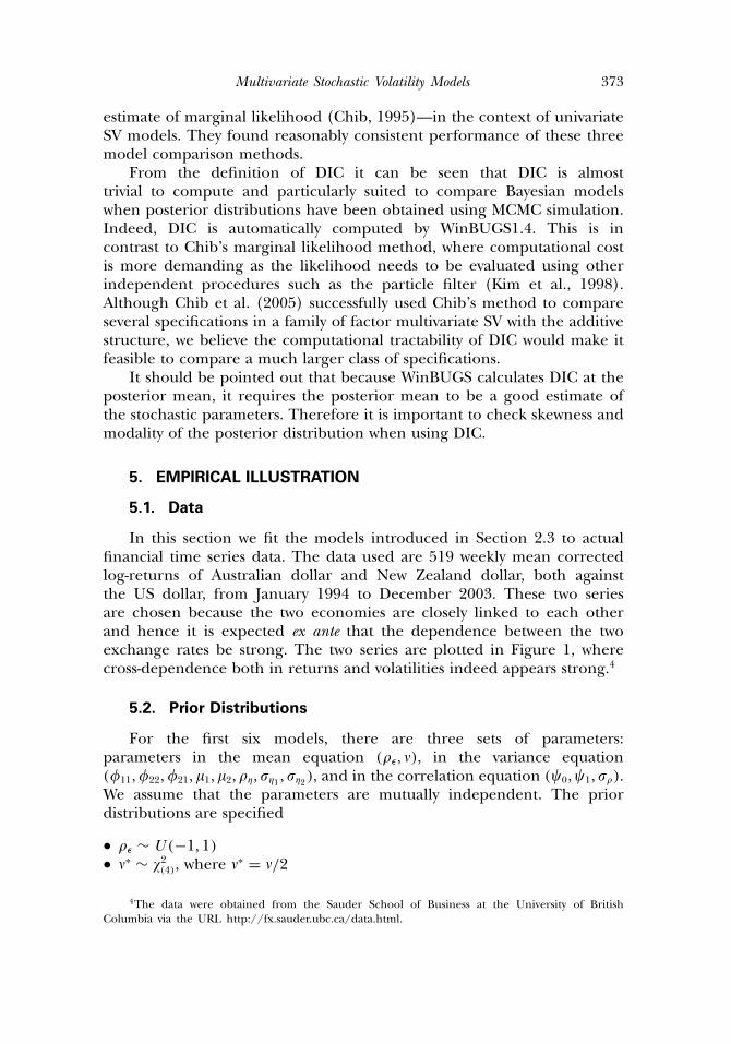
In this section we fit the models introduced in Section 2.3 to actualfinancial time series data. The data used are 519 weekly mean correctedlog-returns of Australian dollar and New Zealand dollar, both againstthe US dollar, from January 1994 to December 2003. These two seriesare chosen because the two economies are closely linked to each otherand hence it is expected ex ante that the dependence between the twoexchange rates be strong. The two series are plotted in Figure 1, wherecross-dependence both in returns and volatilities indeed appears strong.4
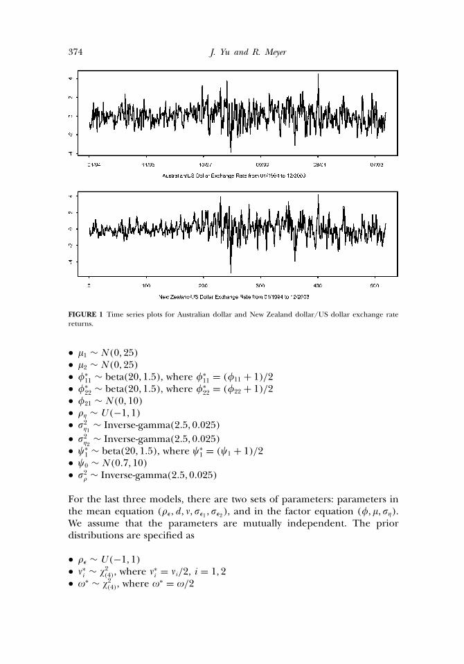
5.2. Prior Distributions
For the first six models, there are three sets of parameters:parameters in the mean equation (�, �), in the variance equation(�11,�22,�21, �1, �2, �, �1 , �2), and in the correlation equation (�0,�1, ).We assume that the parameters are mutually independent. The priordistributions are specified
• � ∼ U (−1, 1)• �∗ ∼ �2(4), where �∗ = �/2
4The data were obtained from the Sauder School of Business at the University of BritishColumbia via the URL http://fx.sauder.ubc.ca/data.html.
374 J. Yu and R. Meyer
FIGURE 1 Time series plots for Australian dollar and New Zealand dollar/US dollar exchange ratereturns.
• �1 ∼ N (0, 25)• �2 ∼ N (0, 25)• �∗
11 ∼ beta(20, 1�5), where �∗11 = (�11 + 1)/2
• �∗22 ∼ beta(20, 1�5), where �∗
22 = (�22 + 1)/2• �21 ∼ N (0, 10)• � ∼ U (−1, 1)• 2
�1∼ Inverse-gamma(2�5, 0�025)
• 2�2
∼ Inverse-gamma(2�5, 0�025)• �∗
1 ∼ beta(20, 1�5), where �∗1 = (�1 + 1)/2
• �0 ∼ N (0�7, 10)• 2
∼ Inverse-gamma(2�5, 0�025)
For the last three models, there are two sets of parameters: parameters inthe mean equation (�, d , �, �1 , �2), and in the factor equation (�, �, �).We assume that the parameters are mutually independent. The priordistributions are specified as
• � ∼ U (−1, 1)• �∗
i ∼ �2(4), where �∗i = �i/2, i = 1, 2
• �∗ ∼ �2(4), where �∗ = �/2
Multivariate Stochastic Volatility Models 375
TABLE 1 Means and standard deviations of prior distributions for parameters in the first sixmodels
� � �11 �22 �21 �1 �2 � �1 �2 �0 �
Prior mean 0 8 .86 .86 0 0 0 0 .12 .12 .7 .86 .12Prior SD .86 4 .11 .11 .33 5 5 .86 .05 .05 3.3 .11 .05
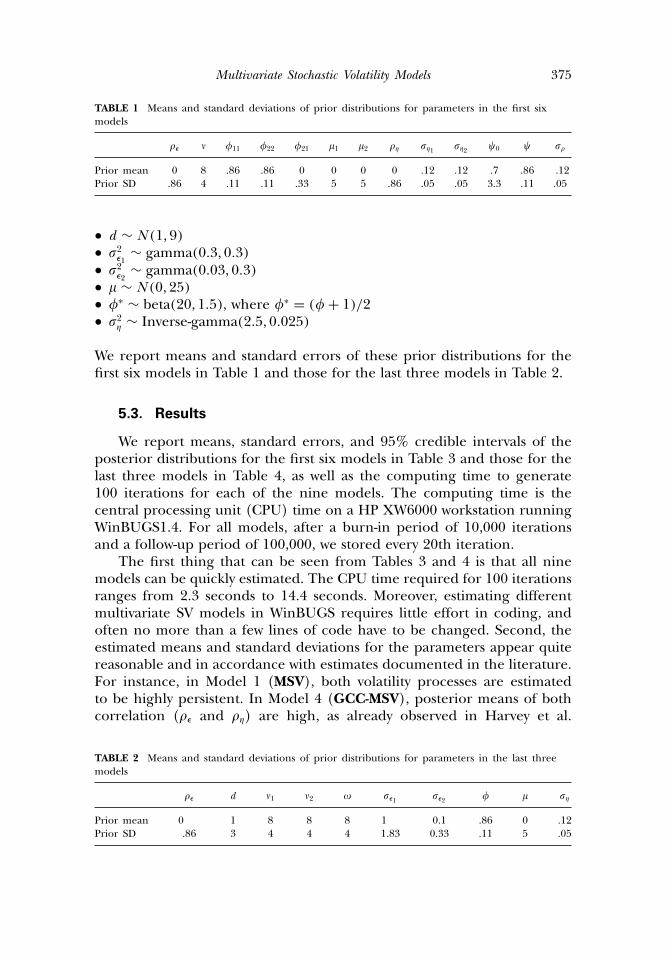
• d ∼ N (1, 9)• 2
�1∼ gamma(0�3, 0�3)
• 2�2
∼ gamma(0�03, 0�3)• � ∼ N (0, 25)• �∗ ∼ beta(20, 1�5), where �∗ = (� + 1)/2• 2
� ∼ Inverse-gamma(2�5, 0�025)
We report means and standard errors of these prior distributions for thefirst six models in Table 1 and those for the last three models in Table 2.
5.3. Results
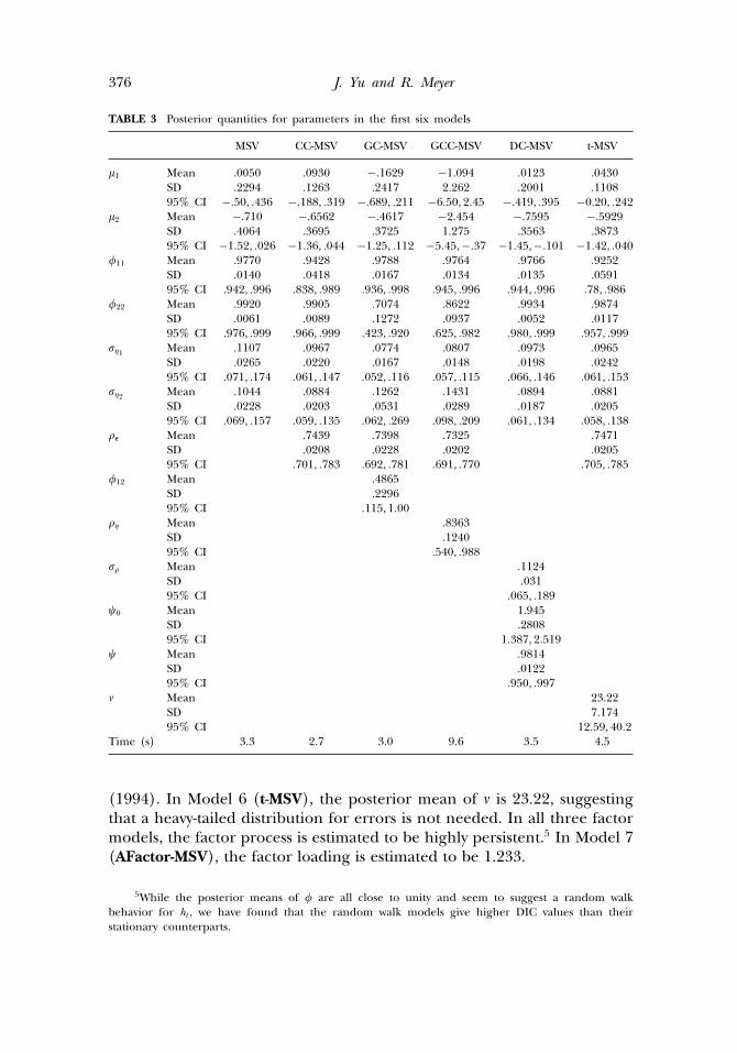
We report means, standard errors, and 95% credible intervals of theposterior distributions for the first six models in Table 3 and those for thelast three models in Table 4, as well as the computing time to generate100 iterations for each of the nine models. The computing time is thecentral processing unit (CPU) time on a HP XW6000 workstation runningWinBUGS1.4. For all models, after a burn-in period of 10,000 iterationsand a follow-up period of 100,000, we stored every 20th iteration.
The first thing that can be seen from Tables 3 and 4 is that all ninemodels can be quickly estimated. The CPU time required for 100 iterationsranges from 2.3 seconds to 14.4 seconds. Moreover, estimating differentmultivariate SV models in WinBUGS requires little effort in coding, andoften no more than a few lines of code have to be changed. Second, theestimated means and standard deviations for the parameters appear quitereasonable and in accordance with estimates documented in the literature.For instance, in Model 1 (MSV), both volatility processes are estimatedto be highly persistent. In Model 4 (GCC-MSV), posterior means of bothcorrelation (� and �) are high, as already observed in Harvey et al.
TABLE 2 Means and standard deviations of prior distributions for parameters in the last threemodels
� d �1 �2 � �1 �2 � � �
Prior mean 0 1 8 8 8 1 0.1 .86 0 .12Prior SD .86 3 4 4 4 1.83 0.33 .11 5 .05
376 J. Yu and R. Meyer
TABLE 3 Posterior quantities for parameters in the first six models
MSV CC-MSV GC-MSV GCC-MSV DC-MSV t-MSV
�1 Mean .0050 .0930 −.1629 −1.094 .0123 .0430SD .2294 .1263 .2417 2.262 .2001 .110895% CI −�50, �436 −�188, �319 −�689, �211 −6�50, 2�45 −�419, �395 −0�20, �242
�2 Mean −.710 −.6562 −.4617 −2.454 −.7595 −.5929SD .4064 .3695 .3725 1.275 .3563 .387395% CI −1�52, �026 −1�36, �044 −1�25, �112 −5�45,−�37 −1�45,−�101 −1�42, �040
�11 Mean .9770 .9428 .9788 .9764 .9766 .9252SD .0140 .0418 .0167 .0134 .0135 .059195% CI �942, �996 �838, �989 �936, �998 �945, �996 �944, �996 �78, �986
�22 Mean .9920 .9905 .7074 .8622 .9934 .9874SD .0061 .0089 .1272 .0937 .0052 .011795% CI �976, �999 �966, �999 �423, �920 �625, �982 �980, �999 �957, �999
�1 Mean .1107 .0967 .0774 .0807 .0973 .0965SD .0265 .0220 .0167 .0148 .0198 .024295% CI �071, �174 �061, �147 �052, �116 �057, �115 �066, �146 �061, �153
�2 Mean .1044 .0884 .1262 .1431 .0894 .0881SD .0228 .0203 .0531 .0289 .0187 .020595% CI �069, �157 �059, �135 �062, �269 �098, �209 �061, �134 �058, �138
� Mean .7439 .7398 .7325 .7471SD .0208 .0228 .0202 .020595% CI �701, �783 �692, �781 �691, �770 �705, �785
�12 Mean .4865SD .229695% CI �115, 1�00
� Mean .8363SD .124095% CI �540, �988
Mean .1124SD .03195% CI �065, �189
�0 Mean 1.945SD .280895% CI 1�387, 2�519
� Mean .9814SD .012295% CI �950, �997
� Mean 23.22SD 7.17495% CI 12�59, 40�2
Time (s) 3.3 2.7 3.0 9.6 3.5 4.5
(1994). In Model 6 (t-MSV), the posterior mean of � is 23.22, suggestingthat a heavy-tailed distribution for errors is not needed. In all three factormodels, the factor process is estimated to be highly persistent.5 In Model 7(AFactor-MSV), the factor loading is estimated to be 1.233.
5While the posterior means of � are all close to unity and seem to suggest a random walkbehavior for ht , we have found that the random walk models give higher DIC values than theirstationary counterparts.
Multivariate Stochastic Volatility Models 377
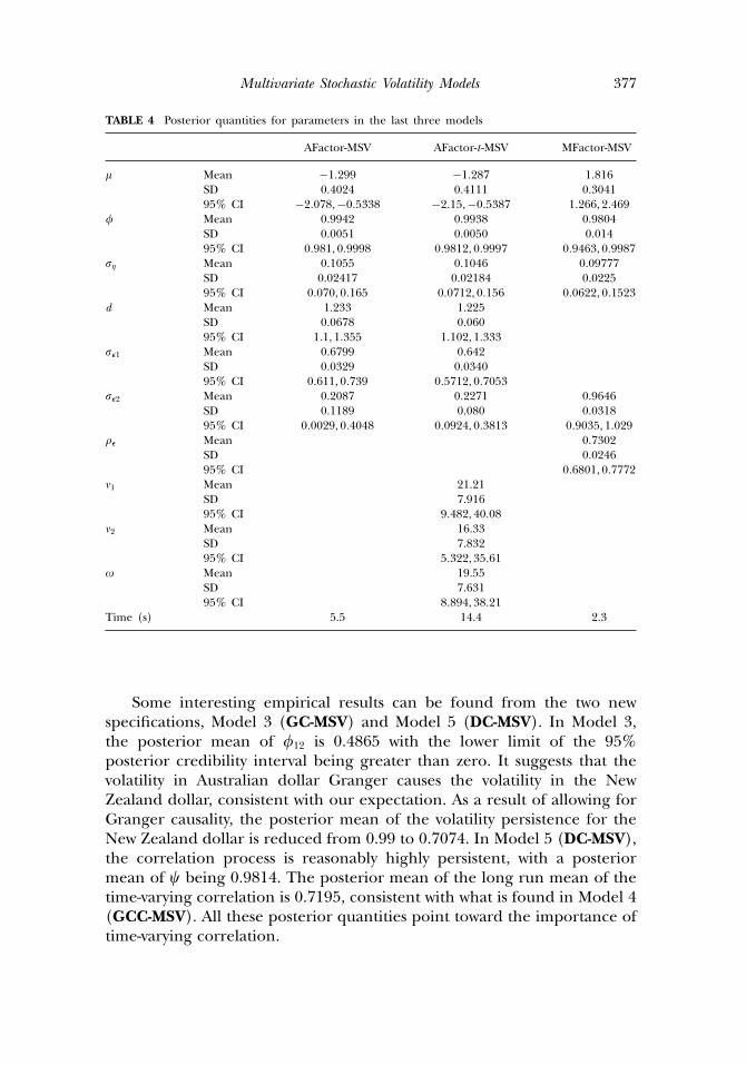
TABLE 4 Posterior quantities for parameters in the last three models
AFactor-MSV AFactor-t -MSV MFactor-MSV
� Mean −1�299 −1�287 1�816SD 0.4024 0.4111 0.304195% CI −2�078,−0�5338 −2�15,−0�5387 1�266, 2�469
� Mean 0.9942 0.9938 0.9804SD 0.0051 0.0050 0.01495% CI 0�981, 0�9998 0�9812, 0�9997 0�9463, 0�9987
� Mean 0.1055 0.1046 0.09777SD 0.02417 0.02184 0.022595% CI 0�070, 0�165 0�0712, 0�156 0�0622, 0�1523
d Mean 1.233 1.225SD 0.0678 0.06095% CI 1�1, 1�355 1�102, 1�333
�1 Mean 0.6799 0.642SD 0.0329 0.034095% CI 0�611, 0�739 0�5712, 0�7053
�2 Mean 0.2087 0.2271 0.9646SD 0.1189 0.080 0.031895% CI 0�0029, 0�4048 0�0924, 0�3813 0�9035, 1�029
� Mean 0.7302SD 0.024695% CI 0�6801, 0�7772
�1 Mean 21.21SD 7.91695% CI 9�482, 40�08
�2 Mean 16.33SD 7.83295% CI 5�322, 35�61
� Mean 19.55SD 7.63195% CI 8�894, 38�21
Time (s) 5.5 14.4 2.3
Some interesting empirical results can be found from the two newspecifications, Model 3 (GC-MSV) and Model 5 (DC-MSV). In Model 3,the posterior mean of �12 is 0.4865 with the lower limit of the 95%posterior credibility interval being greater than zero. It suggests that thevolatility in Australian dollar Granger causes the volatility in the NewZealand dollar, consistent with our expectation. As a result of allowing forGranger causality, the posterior mean of the volatility persistence for theNew Zealand dollar is reduced from 0.99 to 0.7074. In Model 5 (DC-MSV),the correlation process is reasonably highly persistent, with a posteriormean of � being 0.9814. The posterior mean of the long run mean of thetime-varying correlation is 0.7195, consistent with what is found in Model 4(GCC-MSV). All these posterior quantities point toward the importance oftime-varying correlation.
378 J. Yu and R. Meyer
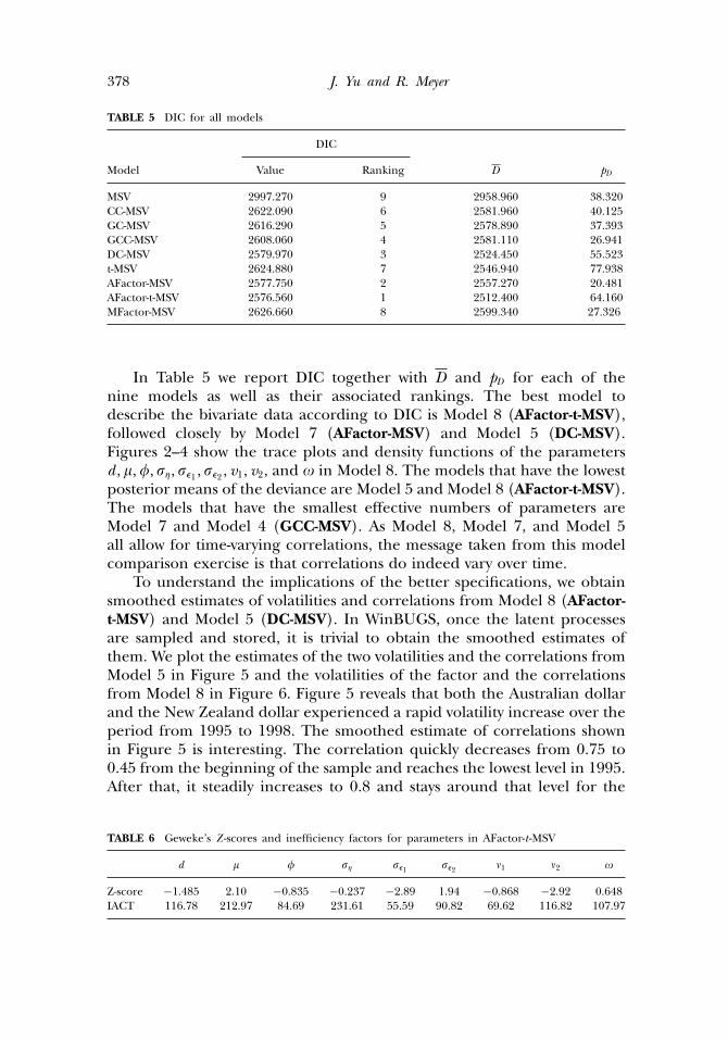
TABLE 5 DIC for all models
DIC
Model Value Ranking D pD
MSV 2997.270 9 2958.960 38.320CC-MSV 2622.090 6 2581.960 40.125GC-MSV 2616.290 5 2578.890 37.393GCC-MSV 2608.060 4 2581.110 26.941DC-MSV 2579.970 3 2524.450 55.523t-MSV 2624.880 7 2546.940 77.938AFactor-MSV 2577.750 2 2557.270 20.481AFactor-t-MSV 2576.560 1 2512.400 64.160MFactor-MSV 2626.660 8 2599.340 27.326
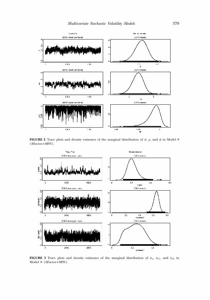
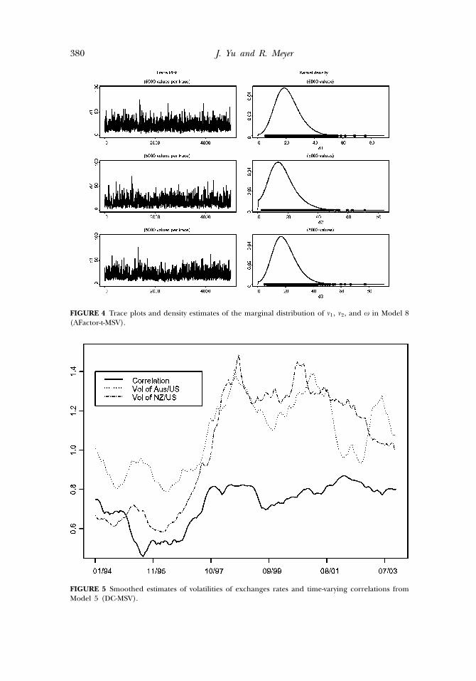
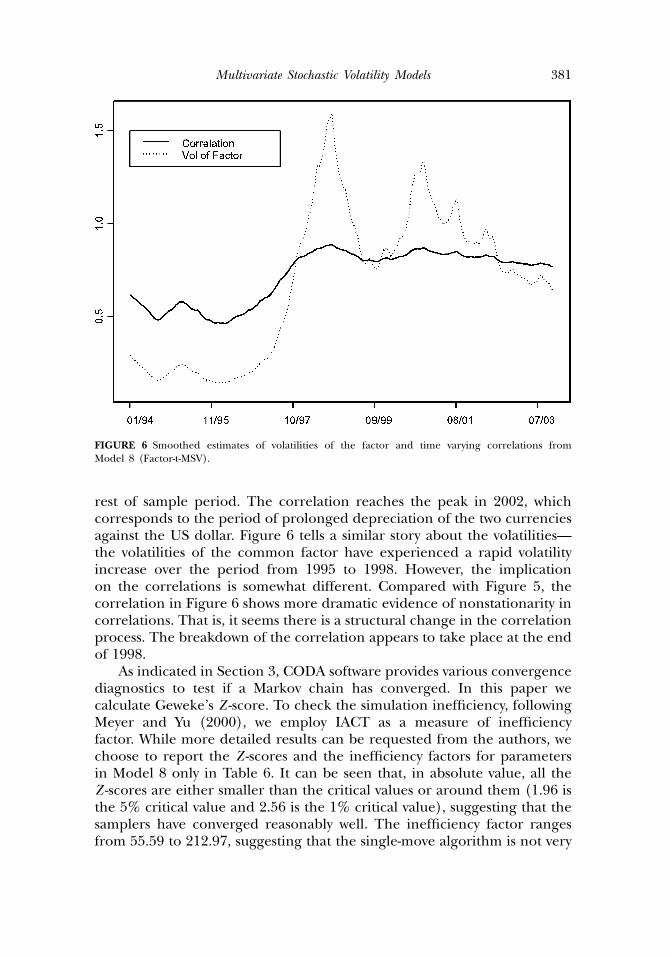
In Table 5 we report DIC together with D and pD for each of thenine models as well as their associated rankings. The best model todescribe the bivariate data according to DIC is Model 8 (AFactor-t-MSV),followed closely by Model 7 (AFactor-MSV) and Model 5 (DC-MSV).Figures 2–4 show the trace plots and density functions of the parametersd , �,�, �, �1 , �2 , v1, v2, and � in Model 8. The models that have the lowestposterior means of the deviance are Model 5 and Model 8 (AFactor-t-MSV).The models that have the smallest effective numbers of parameters areModel 7 and Model 4 (GCC-MSV). As Model 8, Model 7, and Model 5all allow for time-varying correlations, the message taken from this modelcomparison exercise is that correlations do indeed vary over time.
To understand the implications of the better specifications, we obtainsmoothed estimates of volatilities and correlations from Model 8 (AFactor-t-MSV) and Model 5 (DC-MSV). In WinBUGS, once the latent processesare sampled and stored, it is trivial to obtain the smoothed estimates ofthem. We plot the estimates of the two volatilities and the correlations fromModel 5 in Figure 5 and the volatilities of the factor and the correlationsfrom Model 8 in Figure 6. Figure 5 reveals that both the Australian dollarand the New Zealand dollar experienced a rapid volatility increase over theperiod from 1995 to 1998. The smoothed estimate of correlations shownin Figure 5 is interesting. The correlation quickly decreases from 0.75 to0.45 from the beginning of the sample and reaches the lowest level in 1995.After that, it steadily increases to 0.8 and stays around that level for the
TABLE 6 Geweke’s Z -scores and inefficiency factors for parameters in AFactor-t -MSV
d � � � �1 �2 �1 �2 �
Z-score −1.485 2.10 −0.835 −0.237 −2.89 1.94 −0.868 −2.92 0.648IACT 116.78 212.97 84.69 231.61 55.59 90.82 69.62 116.82 107.97
Multivariate Stochastic Volatility Models 379
FIGURE 2 Trace plots and density estimates of the marginal distribution of d , �, and � in Model 8(AFactor-t-MSV).
FIGURE 3 Trace plots and density estimates of the marginal distribution of �, �1, and �2 inModel 8 (AFactor-t-MSV).
380 J. Yu and R. Meyer
FIGURE 4 Trace plots and density estimates of the marginal distribution of �1, �2, and � in Model 8(AFactor-t-MSV).
FIGURE 5 Smoothed estimates of volatilities of exchanges rates and time-varying correlations fromModel 5 (DC-MSV).
Multivariate Stochastic Volatility Models 381
FIGURE 6 Smoothed estimates of volatilities of the factor and time varying correlations fromModel 8 (Factor-t-MSV).
rest of sample period. The correlation reaches the peak in 2002, whichcorresponds to the period of prolonged depreciation of the two currenciesagainst the US dollar. Figure 6 tells a similar story about the volatilities—the volatilities of the common factor have experienced a rapid volatilityincrease over the period from 1995 to 1998. However, the implicationon the correlations is somewhat different. Compared with Figure 5, thecorrelation in Figure 6 shows more dramatic evidence of nonstationarity incorrelations. That is, it seems there is a structural change in the correlationprocess. The breakdown of the correlation appears to take place at the endof 1998.
As indicated in Section 3, CODA software provides various convergencediagnostics to test if a Markov chain has converged. In this paper wecalculate Geweke’s Z -score. To check the simulation inefficiency, followingMeyer and Yu (2000), we employ IACT as a measure of inefficiencyfactor. While more detailed results can be requested from the authors, wechoose to report the Z -scores and the inefficiency factors for parametersin Model 8 only in Table 6. It can be seen that, in absolute value, all theZ -scores are either smaller than the critical values or around them (1.96 isthe 5% critical value and 2.56 is the 1% critical value), suggesting that thesamplers have converged reasonably well. The inefficiency factor rangesfrom 55.59 to 212.97, suggesting that the single-move algorithm is not very
382 J. Yu and R. Meyer
efficient and a long sample is needed. When we increase the number ofiterations to 500,000, however, the empirical results remain essentially thesame.
6. CONCLUSION
In this paper we proposed to estimate and compare multivariateSV models using Bayesian MCMC techniques via WinBUGS. MCMC isa powerful method and has a number of advantages over alternativemethods. Unfortunately, writing the first MCMC program for estimatingmultivariate SV models is not easy, and comparing alternative multivariateSV specifications is computationally costly. WinBUGS imposes a shortbut sharp learning curve. In the bivariate setting, we show that itsimplementation is easy and computationally reasonably fast. Also, it is veryflexible to handle a rich class of specifications. However, since WinBUGSoffers a single-move Gibbs sampling algorithm, as one would expect, wefind that the mixing is generally slow and hence a long sample is required.
We illustrated the implementation in WinBUGS by exploringand comparing nine bivariate models, including Granger causality involatilities, time-varying correlations, heavy-tailed error distributions,additive factor structure, and multiplicative factor structure, two of whichare new to the SV literature. Our empirical results based on weeklyAustralian/US dollar and New Zealand/US dollar exchange rates indicatethat the models that allow for time-varying coefficients generally fit thedata better.
ACKNOWLEDGMENTS
Jun Yu gratefully acknowledges financial support from the Wharton-SMU Research Center and computing support from the Center forAcademic Computing, both at Singapore Management University. Theresearch of the second author was supported by the Royal Society of NewZealand Marsden Fund. We also wish to thank two referees for constructivecomments, and Manabu Asai, Ching-Fan Chung, Mike McAleer, Yiu KuenTse, and seminar participants at the Workshop on Econometric Theory andApplications in Taiwan for helpful discussion.
REFERENCES
Aas, K., Haff, I. (2006). The generalized hyperbolic skew student’s t -distribution. Journal of FinancialEconometrics 4:275–309.
Aguilar, O., West, M. (2000). Bayesian dynamic factor models and portfolio allocation. Journal ofBusiness and Economic Statistics 18:338–357.
Akaike, H. (1973). Information theory and an extension of the maximum likelihood principle.In: Proceedings 2nd International Symposium Information Theory. Petrov, B. N., Csaki, F., eds.Budapest: Akademiai Kiado, pp. 267–281.
Multivariate Stochastic Volatility Models 383
Andersen, T., Sorensen, B. (1996). GMM estimation of a stochastic volatility model: a Monte Carlostudy. Journal of Business and Economic Statistics 14:329–352.
Andersen, T., Chung, H., Sorensen, B. (1999). Efficient method of moments estimation of astochastic volatility model: a Monte Carlo study. Journal of Econometrics 91:61–87.
Asai, M., McAleer, M. (2005). The structure of dynamic correlations in multivariate stochasticvolatility models. Faculty of Economics. Japan: Saka University.
Asai, M., McAleer, M., Yu, J. (2006). Multivariate stochastic volatility models: a survey. 24(2–3):443–473.
Bauwens, L., Laurent, S., Rombouts, J. V. K. (2006). Multivariate GARCH: A survey. Journal of AppliedEconometrics 21:79–109.
Berg, A., Meyer, R., Yu, J. (2004). Deviance information criterion for comparing stochastic volatilitymodels. Journal of Business and Economic Statistics 22:107–120.
Bollerslev, T. (1990). Modelling the coherence in shirt-run nominal exchange rates: a multivariategeneralized ARCH approach. Review of Economics and Statistics 72:498–505.
Bollerslev, T., Engle, R., Wooldridge, J. M. (1998). A capital asset pricing model with time varyingcovariances. Journal of Political Economy 96:116–131.
Braun, P., Nelson, D., Sunier, A. (1995). Good news, bad news, volatility and betas. Journal of Finance50:1575–1603.
Chan, D., Kohn, R., Kirby, C. (2005). Multivariate stochastic volatility with leverage. EconometricReviews 25(2–3):245–274.
Chib, S. (1995). Marginal likelihood from the Gibbs output. Journal of the American StatisticalAssociation 90:1313–1321.
Chib, S., Nardari, F., Shephard, N. (2005). Analysis of high dimensional multivariate stochasticvolatility models. Journal of Econometrics, forthcoming.
Christodoulakis, G., Satchell, S. E. (2002). Correlated ARCH (CorrARCH): modelling the time-varying conditional correlation between fianacial asset returns. European Journal of OperationalResearch 139:351–370.
Danielsson, J. (1994). Stochastic volatility in asset prices: estimation with simulated maximumlikelihood. Journal of Econometrics 64:375–400.
Danielsson, J. (1998). Multivariate stochastic volatility models: estimation and comparison withVGARCH models. Journal of Empirical Finance 5:155–173.
Diebold, F. X., Nerlove, M. (1989). The dynamics of exchange rate volatility: a multivariate latent-factor ARCH model. Journal of Applied Econometrics 4:1–22.
Ding, Z., Engle, R. (2001). Large scale conditional covariance modelling, estimation and testing.Academia Economic Papers 29:157–184.
Durham, G. S. (2005). Monte Carlo methods for estimating, smoothing, and filtering one and two-factor stochastic volatility models. Journal of Econometrics, forthcoming.
Engle, R. (2002). Dynamic conditional correlation—a simple class of multivariate GARCH models.Journal of Business and Economic Statistics 17:239–250.
Engle, R., Kroner, K. (1995). Multivariate simultaneous GARCH. Econometric Theory 11:122–150.Engle, R., Ng, V., Rothschild, M. (1990). Asset pricing with a factor ARCH covariance structure:
empirical estimates for treasury bills. Journal of Econometrics 45:213–237.Fridman, M., Harris, L. (1998). A maximum likelihood approach for non-Gaussian stochastic
volatility models. Journal of Business and Economic Statistics 16:284–291.Gilks, W. (1992). Derivative-free adaptive rejection sampling for Gibbs sampling. In: Bayesian Statistics
4. Bernardo, J. M., Berger, J. O., Dawid, A. P., Smith, A. F. M., eds. Oxford: Oxford UniversityPress, pp. 642–665.
Harvey, A. C. (1990). Forecasting, Structural Time Series Models and the Kalman Filter. New York:Cambridge University Press.
Harvey, A. C., Ruiz, E., Shephard, N. (1994). Multivariate stochastic variance models. Review ofEconomic Studies 61:247–264.
Jacquier, E., Polson, N. G., Rossi, P. E. (1994). Bayesian analysis of stochastic volatility models. Journalof Business and Economic Statistics 12:371–389.
Jacquier, E., Polson, N. G., Rossi, P. E. (1995). Priors and models of stochastic volatility models.Unpublished manuscript, University of Chicago.
Jacquier, E., Polson, N. G., Rossi, P. E. (1999). Stochastic volatility: univariate and multivariateextensions. Unpublished manuscript, University of Chicago.
384 J. Yu and R. Meyer
Jungbacker, B., Koopman, S. J. (2006). Monte Carlo likelihood estimation for three multivariatestochastic volatility models. Econometric Reviews 25(2–3):385–408.
Kim, S., Shephard, N., Chib, S. (1998). Stochastic volatility: Likelihood inference and comparisonwith ARCH models. Review of Economic Studies 65:361–393.
Knight, J. L., Satchell, S. S., Yu, J. (2002). Estimation of the stochastic volatility model by theempirical characteristic function method. Australian and New Zealand Journal of Statistics44:319–335.
Lancaster, T. (2004). An Introduction to Modern Bayesian Econometrics. Oxford: Blackwell.Liesenfeld, R., Richard, J. (2003). Univariate and multivariate stochastic volatility models: estimation
and diagnostics. Journal of Empirical Finance 10:505–531.McAleer, M. (2005). Automated inference and learning in modelling financial volatility. Econometric
Theory 21:232–261.Melino, A., Turnbull, S. M. (1990). Pricing foreign currency options with stochastic volatility. Journal
of Econometrics 45:239–265.Meyer, R., Yu, J. (2000). BUGS for a Bayesian analysis of stochastic volatility models. Econometrics
Journal 3:198–215.Meyer, R., Fournier, D. A., Berg, A. (2003). Stochastic volatility: Bayesian computation using
automatic differentiation and the extended Kalman filter. Econometrics Journal 6:408–420.Neal, R. (1997). Markov chain Monte Carlo methods based on “slicing” the density function.
Technical Report 9722. Department of Statistics, University of Toronto, Canada.Neal, R. (1998). Suppressing random walks in Markov chain Monte Carlo methods using ordered
over-relaxation. In: Learning in Graphical Models. Jordan, M. I., ed. Dordrecht: KluwerAcademic Publishers, pp. 205–230.
Newton, M., Raftery, A. E. (1994). Approximate Bayesian inferences by the weighted likelihoodbootstrap. Journal of the Royal Statistical Society, Series B 56:3–48 (with discussion).
Pitt, M., Shephard, N. (1999). Time varying covariances: a factor stochastic volatility approach. In:Bernardo, J. M., Berger, J. O., David, A. P., Smith, A. F. M., eds. Bayesian Statistics 6. Oxford:Oxford University Press, pp. 547–570.
Quintana, J. M., West, M. (1987). An analysis of international exchange rates using multivariateDLMs. Statistician 36:275–281.
Richard, J. F., Zhang, W. (2004). Efficient high-dimensional importance sampling. Working paper,University of Pittsburgh.
Sandmann, G., Koopman, S. J. (1998). Maximum likelihood estimation of stochastic volatility models.Journal of Econometrics 63:289–306.
Selçuk, F. (2004). Free float and stochastic volatility: the experience of a small open economy.Physica A 342:693–700.
Shephard, N. (2005). Stochastic Volatility: Selected Readings. Oxford: Oxford University Press.Spiegelhalter, D. J., Thomas, A., Best, N. G., Gilks, W. R. (1996). BUGS 0.5, Bayesian Inference Using
Gibbs Sampling. Manual (version ii). MRC Biostatistics Unit, Cambridge, UK.Spiegelhalter, D. J., Best, N. G., Carlin, B. P., van der Linde, A. (2002). Bayesian measures of model
complexity and fit (with discussion). Journal of the Royal Statistical Society, Series B 64:583–639.Spiegelhalter, D. J., Thomas, A., Best, N. G., Gilks, W. R. (2003). WinBUGS User Manual (Version 1.4).
MRC Biostatistics Unit, Cambridge, UK.Tsay, R. S. (2002). Analysis of Financial Time Series. New York: John Wiley.Tse, Y., Tusi, A. (2002). A multivariate GARCH model with time-varying correlations. Journal of
Business and Economic Statistics 17:351–362.Yu, J. (2002). Forecasting volatility in the New Zealand stock market. Applied Financial Economics
12:193–202.Yu, J. (2005). On leverage in a stochastic volatility model. Journal of Econometrics 127:165–178.