ANALYSIS OF STOCHASTIC AND NON-STOCHASTIC VOLATILITY MODELS

A THESIS SUBMITTED TO THE GRADUATE SCHOOL OF NATURAL AND APPLIED SCIENCES

OF MIDDLE EAST TECHNICAL UNIVERSITY

BY

PEL�N ÖZKAN

IN PARTIAL FULFILLMENT OF THE REQUIREMENTS FOR THE DEGREE OF MASTER OF SCIENCE

IN

STATISTICS

SEPTEMBER 2004

Approval of the Graduate School of Natural and Applied Sciences.

Prof. Dr. Canan Özgen

Director

I certify that this thesis satisfies all the requirements as a thesis for the degree of

Master of Science.

Prof. Dr. H. Özta� Ayhan

Head of Department

We certify that we have read this thesis and that in our opinion it is fully adequate, in

scope and quality, as a thesis for the degree of Master of Science.

Zafer Ali Yavan Prof. Dr. Özta� Ayhan

Co-Supervisor Supervisor

Examining Committee Members

Prof. Dr. H. Özta� Ayhan (METU, STAT)

Assoc. Prof. Dr. Bilgehan Güven (METU, STAT)

Asst. Prof. Dr. �nci Batmaz (METU, STAT)

Zafer Ali Yavan (TÜS�AD)

Dr. Barı� Sürücü (METU, STAT)

iii

I hereby declare that all information in this document has been obtained and

presented in accordance with academic rules and ethical conduct. I also

declare that, as required by these rules and conduct, I have fully cited and

referenced all material and results that are not original to this work. Pelin ÖZKAN

iv

ABSTRACT

ANALYSIS OF STOCHASTIC AND NON-STOCHASTIC VOLATILITY

MODELS

ÖZKAN, Pelin

M.S., Department of Statistics

Supervisor: Prof. Dr. H. Özta� AYHAN

Co-Supervisor: Zafer Ali Yavan

September 2004, 64 pages

Changing in variance or volatility with time can be modeled as

deterministic by using autoregressive conditional heteroscedastic (ARCH) type

models, or as stochastic by using stochastic volatility (SV) models. This study

compares these two kinds of models which are estimated on Turkish / USA

exchange rate data. First, a GARCH(1,1) model is fitted to the data by using the

package E-views and then a Bayesian estimation procedure is used for estimating

an appropriate SV model with the help of Ox code. In order to compare these

models, the LR test statistic calculated for non-nested hypotheses is obtained.

Key Words: Volatility, ARCH models, GARCH models, M-GARCH models,

v

E-GARCH models, SV models, Monte Carlo integration, Gibbs sampler,

Metropolis-Hasting algorithm, MCMC algorithm.

vi

ÖZ

STOKAST�K VE STOKAST�K OLMAYAN VARYANS MODELLER�N�N

ANAL�Z�

ÖZKAN, Pelin

Yüksek Lisans, �statistik Bölümü

Tez Yöneticisi: Prof. Dr. H. Özta� Ayhan

Ortak Tez Yöneticisi: Zafer Ali Yavan

Eylül 2004, 64 sayfa

Varyansın zaman içerisindeki de�i�imi rasgele olmayan bir �ekilde

otoregresyon ko�ullu de�i�en varyans (ARCH) modelleri ile ya da stokastik olarak

stokastik varyans modelleri ile modellenebilir. Bu çalı�ma, Türkiye /A.B.D döviz

kuru üzerinde tahmin edilen bu iki tür modeli kar�ıla�tırmaktadır. �lk olarak bir

GARCH(1,1) modeli E-views paket programı kullanılarak verilere uyarlanmı�

daha sonra Ox yardımıyla, bayes tahmin yöntemleri kullanılarak uygun bir

stokastik varyans modeli uygulanmı�tır. Bu modelleri kar�ıla�tırmak amacıyla, iç

içe geçmeyen varsayımlar için hesaplanan olasılık oran test istatisti�i elde

edilmi�tir.

vii

Key Words: Varyans, ARCH modelleri, GARCH modelleri, M-GARCH

modelleri, E-GARCH modelleri, SV modelleri, Monte Carlo integral yöntemi,

Gibbs seçicisi, Metropolis-Hasting algoritması, MCMC algoritması.

viii

To my parents for their unconditional love....

ix

ACKNOWLEDGEMENTS

I would like to thank my supervisor Prof. Dr. Özta� Ayhan who gave me the

opportunity to complete my thesis.

I am very much indebted to Zafer Ali Yavan for being my co-supervisor. His

timely suggestions, comments and encouragement were really incentive for me.

I would also like to thank the Chairman of the Department, Prof. Dr. Özta�

Ayhan, on behalf of the Department of Statistics for all of the necessary

equipments to complete this work.

I am grateful to Prof. Dr. Haluk Erlat for his great guidence and also to Prof.

Dr. Anthony Atkinson for answering my very critical questions patiently which

makes me complete this work.

I owe my heartful thanks to Oya Can Mutan who shares an invaluable

friendship with me. Her great understanding and continous support have helped

me to put forth my full effort and to overcome all the difficulties that I came

across during this study.

I would also like to express my deep appreciation to Dr. Hakan Sava� Sazak

due to his important contributions to my work and sincere assistance whenever I

need him.

x

Very special thanks are for Didem Avcıo�lu Aytürk and Dr. Barı� Sürücü for

their lovely and cheerful friendships.

I want to express my loving thanks to my brother, Özgür Özkan for his

complete reliance on me and unbounded support. It was this support which made

my goals achievable. Without him I could hardly have completed this work.

I would also express my sincere appreciate to my sister in-law, Figen Özkan

for her excellent motivitation in many aspects.

I owe an immense dept of gratitude to my parents whose patience and sacrifice

will always be an inspriation for me. The most valuable thing that I could ever

have is their boundless love.

The last but by no means least appreciation is for my love Umut Özbozkurt

who always gives me the courage to follow my dreams and makes everything

meaningful by sharing all the moments of my life.

xi

TABLE OF CONTENTS

PLAGIARISM………………………………………………………………………………… iii

ABSTRACT……………………………………………………………………... iv

ÖZ………………………………………………………………………………...vi

DEDICATION…………………………………………………………………..viii

ACKNOWLEDGEMENTS………………………………………………………ix

TABLE OF CONTENTS…………………………………………………………xi

LIST OF TABLES………………………………………………………………xiii

LIST OF FIGURES……………………………………………………………..xiv

CHAPTER

1. INTRODUCTION…………………………………………………………...1

2. LITERATURE SURVEY…………………………………………………...4

3. BASIC TIME SERIES CONCEPTS……………………………………….12

3.1 Simple Linear Processes……………………………………………….14 3.1.1 White-Noise Processes……………………………………………14 3.1.2 Autoregressive Processes…………………………………………14

xii

3.1.3 Moving Average Processes………………………………………17 3.1.4 Autoregressive Moving Average Processes……………………...19 3.2 Criteria for Model Selection………………………………………….19 3.3 Unit root tests………………………………………………………...21

4. VOLATILITY MODELS…………………………………………………..23

4.1 Autoregressive Conditionally Heteroskedastic (ARCH) Models...........24 4.2 Generalized ARCH (GARCH) Models..................................................27

4.3 GARCH in Mean Models.......................................................................29

4.4 Exponential GARCH Models………………………………………….30

4.5 Stochastic Volatility (SV)……………………………………………...31

4.5.1 SV Estimation…………………………………………………34

4.5.2 Bayesian Theory……………………………………………….34

4.5.3 MCMC for SV…………………………………………………38

5. APPLICATION OF VOLATILITY MODELS ON TURKISH FINANCIAL

DATA………………………………………………………………………42

5.1 Estimation of GARCH models……………………………………..46 5.2 Estimation of SV model…………………………………………….49 5.3 Comparison of GARCH and SV……………………………………51

6. CONCLUSION…………………………………………………………….54

REFERENCES.......................................................................................................56

xiii

LIST OF TABLES

TABLE

5.1 : ADF test statistic without trend component.................................................. 43

5.2 : ADF test statistic with trend component… … … … … … … … … … … … … … 43

5.3 : Unit root test for the difference of TL/Dollar exchange rates… … … … … ....44

5.4 : Test results of autocorrelation… … … … … … … … … … … … … … … … … … 46

5.5 : GARCH (1,1) results for percentage return… … … … … … … … … … … … ...47

5.6 : E-GARCH(1,1) results for percentage return… … … … … … … … … … … … 47

5.7 : M-GARCH(1,1) results for percentage return… … … … … … … … .… … … ..48

5.8 : Estimation results for the SV model..............................................................50

xiv

LIST OF FIGURES

FIGURES

5.1 : Plot of the TL/Dollar exchange rates........................................................... 42

5.2 : Plot of the difference of the TL/Dollar exchange rates.................................44

5.3 : Descriptive statistics for the TL/Dollar exchange rates.................................45

5.4 : Descriptive statistics for the error term under GARCH (1,1) process...........49

5.5 : Descriptive statistics for the error term under SV process.............................51

1

CHAPTER 1

INTRODUCTION

Time series models have been widely used in many disciplines in the

science. Many econometricians and statisticians devote themselves to developed

new models and improve the existing ones. In the last years, there has been

growing interest in time series models with changing variance over time which is

shown by most of the financial data. Such time series models with heteroscedastic

errors are specifically useful for modeling high frequency data like stock returns

and exchange rates. In the simplest case, the series mean of which is considered as

zero is a white noise process with unit variance multiplied by a factor �t known as

volatility (Kuan,2003). That is,

yt = �t�t.

A volatility model is a specification of dynamics of the volatility process.

There are different ways for modeling changes in volatility over time. A

commonly used model is the autoregressive conditionally heteroscedastic

(ARCH) model introduced by Engle (1982) in which the conditional variance is a

function of the squared past values of the series including time t-1. Consequently,

the volatility is observable at time t-1. This model has been extended in different

directions. The most popular of them is generalized autoregressive conditionally

heteroscedastic (GARCH) model which was proposed by Bollerslev after four

years of introduction of ARCH models and it lets conditional variance depend on

2

the squared past observations and previous variances. As well as ARCH models,

in GARCH models the volatility is known at time t-1. However, the volatility may

be treated as an unobserved variable and this yields another class of models which

consider the variance of the process as stochastic and model the logarithm of

volatility as a linear stochastic process such as autoregression. Models of this kind

are called stochastic variance or stochastic volatility (SV) models. The interest in

SV models has been very strong in recent years. These models are important

alternatives to the famous ARCH models. They have similar properties but they

are different with respect to the observability of �t2 at time t-1, that means, the

distinction between the two models relies on whether the volatility is observable

or not. Formally, GARCH models, with one lag, can be expressed as,

�2

t = a0 + �1y2t-1 + b1 �t-1

2,

whereas, SV models can be written as,

ln(�t2) = �0 + �1 ln(�t-1

2) + vt,

The innovation term, vt, of the variance equation let the variance change with time

stochastically.

Although ARCH type models are easier to deal with, allowing volatility

change with time is more realistic and some researchers turned their attention to

this new class of volatility models. SV models are more flexible but more difficult

to estimate than ARCH type models due to the fact that it is not easy to derive

their exact likelihood function and because of this, they have been unattractive

models until the developments of the new estimation methods. Improvements in

computers and programming languages make them important alternatives to the

deterministic volatility processes.

In this study, both classes of volatility models are analyzed. The exchange

rate of TL/$ is considered and suitable deterministic and stochastic volatility

3

models are constructed in order to see which one is better in modeling the time-

varying variance.

The organization of the study is as follows. In chapter 2, the previous

studies on the concept of volatility modeling is described briefly. In chapter 3,

some basic definitions in time series analysis is given. Chapter 4 discusses the

volatility models by dividing them into two parts as deterministic and stochastic.

The empirical example is given in chapter 5 which includes the comparison of

GARCH(1,1) and SV model. The last chapter, chapter 6, concludes all the work

done in this thesis.

4

CHAPTER 2

LITERATURE SURVEY

Analyzing financial time series data with volatility models has become

very common in recent years and a huge literature having been established. One

of the most important tools that characterizes the changing of the variance is the

ARCH model. Engle (1982) proposes to model time-varying conditional variance

with the ARCH process that use past disturbances to model the variance of the

series. Early empirical evidence shows that high ARCH order has to be selected in

order to catch the dynamic of the conditional variance. The GARCH model of

Bollerslev (1986) is an answer to this issue. Several excellent surveys on

ARCH/GARCH models are available in Bollerslev, Chou and Kroner (1992),

Bollerslev, Engle and Nelson (1994) and Bera and Higgins (1993). The maximum

likelihood based inference procedures for the ARCH class of models under

normality assumption are discussed in Engle (1982) and Pantula (1985).

Generalized Method of Moments (GMM) estimation of ARCH type models are

discussed in Mark (1988), Bodurtha and Mark (1991), Glosten, Jagannathan, and

Runkle (1991) and Simon (1989). In addition to these, the Bayesian inference

procedures within the ARCH type of models are developed by Geweke (1988)

who uses Monte Carlo methods to determine the exact posterior distributions. As

an alternative estimation technique, Gallant and Nychka (1987), Gallant, Rossi

and Tauchen (1990) use a semiparametric approach while Robinson (1987),

Pagan and Ullah (1988), Whistler (1988) use a nonparametric method.

5

The search for model specification and selection is always guided by

empirical stylized facts. Stylized facts about volatility have been well documented

in the ARCH literature, for instance in Bollerslev, Engle and Nelson (1994). Since

the early sixties, it was observed by Mandelbrot (1963) and Fama (1965) and

among others that asset returns have leptokurtic distribution with thick tails. As a

result numerous papers have proposed to model the returns from fat-tailed

distributions. In addition to thick tails, the volatility clustering is also common.

ARCH models introduced by Engle (1982) and the numerous extensions as well

as SV models are built to capture this volatility clustering. Leverage effect is

another fact about the financial time series. Leverage effect suggests that stock

price movements are negatively correlated with volatility.

The distribution considered in ARCH and GARCH models is symmetric

and fail to model the third stylized fact, namely the leverage effect. To solve this

problem, many extensions to GARCH models have been proposed. Among the

most widely spread are Exponential GARCH (EGARCH) of Nelson (1991), the so

called GJR of Glosten, Jagannathan, and Runkle (1993) and the Asymmetric

Power ARCH (APARCH) of Ding, Granger and Engle( 1993).

The thick tails property of financial time series data often do not fully

captured by GARCH models. This has naturally led to the use of non normal

distributions to better model this excess kurtosis. Bollerslev (1987), Baillie and

Bollerslev (1989) and Kaiser (1996) use Student–t distribution while Nelson

(1991) and Kaiser (1996) suggest the Generalized Error Distribution (GED).

Other propositions include mixture distributions such as the normal-poison

(Jorion, 1988), the normal-lognormal (Hsieh, 1989) or the Bernoulli-normal(

Vlaar and Palm, 1993). Moreover, to better capture the skewness, Liu and Brorsen

(1995) applies an asymmetric stable density. A promising distribution that models

both the skewness and kurtosis is the skewed Student-t of Fernandez and Steel

(1998), extended to the GARCH framework by Lambert and Laurent (2000).

6

The other well known volatility model is ARCH- in Mean or ARCH-M

model introduced by Engle, Lilien, and Robins (1987), who considers the

conditional mean equation is a function of the conditional variance. In this model,

an increase in conditional variance will be associated with an increase or a

decrease in the conditional mean of the process.

The other specifications for �t2 are as follows, the Taylor (1986) /

Schewert (1989) (TS-GARCH) model, the A-GARCH, the NA-GARCH and the

V-GARCH models suggested by Engle and Ng (1993), the threshold GARCH

model (Thr-GARCH) by Zakoinan (1994), the log-ARCH by Geweke (1986) and

Pantula (1986), the integrated GARCH (IGARCH) model due to Engle and

Bollerslev (1986), the NARCH of Higgins and Bera (1992), the GQ_GARCH

suggested by Sentana (1995) and finally the Aug-GARCH suggested by Duan

(1997). The formulation of various ARCH/GARCH models is given in Table 2.1.

7

Table 2.1 ARCH-type models

ARCH: �=

−+=q

itit

1

21

2 εαωσ

GARCH: � �= =

−− ++=q

i

p

ijtjtit

1 1

221

2 σβεαωσ

IGARCH: � �= =

−−−−− −+−++=q

i

p

jtjtjtititt

2 1

21

221

221

2 )()( εσβεεαεωσ

Taylor/Schwert: jt

q

i

p

ijjtit −

= =−� �++= σβεαωσ

1 1

||

A-GARCH: [ ]� �=

−−− +++=q

i

p

jjtjitiitit

01 1

222 σβεγεαωσ

GJR-GARCH: [ ]� �= =

−−> +++=−

q

i

p

jjtjitiit it

I1 1

22)0(

2 σβεγαωσ ε

log-GARCH*: � �= =

−− ++=q

i

p

jjtjitit e

1 1

)log(||)log( σβαωσ

NGARCH: ��=

−=

− ++=p

jjtj

q

iitit

11

|| δδδ σβεαωσ

A-PARCH: [ ] ��=

−=

−− +−+=p

jjtj

q

iitiitit

11

|| δδδ σβεγεαωσ

* et is the standardized returns

8

A comparison of 330 different ARCH-type models in terms of their ability

to describe the conditional variance is given in Hansen and Lunde (2003). The

main findings are that there is no evidence that a GARCH(1,1) model is

outperformed by other models.

Over the last decade, there has been a tendency to employ the ARCH type

models to analyze the volatilities of financial data while ignoring the specification

and estimation of the conditional mean. Most recently, Li, Ling and McAleer

(2002) define the ARMA-GARCH model which can be reduced to ARMA-

ARCH, AR-ARCH, MA-ARCH by simply imposing some restrictions to the

process.

The ARCH type models are generalized to the multivariate case by

Bollerslev, Engle and Wooldridge in 1988. This model is estimated by maximum

likelihood, however, the number of parameters can be very large, so it is usually

necessary to impose restrictions. Bollerslev (1990) mentions about these

restrictions.

Another type of volatility process is stochastic volatility model. Due to the

fact that in SV models the mean and the variance are driven by separate stochastic

process, SV models are much harder to estimate than the GARCH models.

Evaluating the likelihood function of ARCH type models is a relatively easy task.

In contrast, for SV model, it is impossible to obtain explicit expression for the

likelihood function. The lack of estimation procedures for SV models made them

for a long time an unattractive class of models in comparison to ARCH type

models. In recent years, however, several estimation methods have been

developed with the increasing performance of the programming languages and

computers. The early attempts to estimate SV models used a GMM procedure due

to Melino and Turnbull (1990). GMM considers the basic SV model with normal

innovation processes. In general, m moments are computed. For a sample size of

T, let gT(�) denotes the m x 1 vector of differences between each sample moment

9

and its theoretical expression in terms of the model parameters �. The GMM

estimator is constructed by minimizing the function,

)()(minˆ ' βββ TTTt gWg= ,

where WT is an m x m matrix reflecting the importance given to matching each

moments. When the innovation terms are independent, Jacquier, Polson and Rossi

(1994) suggest using 24 moments. The GMM method may also be extended to

handle a non-normal distribution which is done in Andersen (1994). The

inefficiency of the GMM estimation is proved by Andersen and Sorensen (1993)

and Jacquier, Polson and Rossi (1994).

Another estimation method is called quasi-maximum likelihood estimation

developed by Harvey, Ruiz and Shephard (1994). A key feature of the basic SV

model is that it can be transformed into a linear model by taking the logarithm of

the squares of the observations. The resulting error term, log�t2, is log of a chi-

square distribution with one degree of freedom which is highly left-skewed.

Harvey, Ruiz and Shephard (1994) have employed Kalman filtering to estimate

the parameters by maximizing the quasi likelihood function.

Comparison of GMM and QML can be found in Ruiz (1994), Harvey and

Shephard(1995). The general conclusion is QML gives estimates with smaller

mean square error.

The GMM and QML methods do not involve simulations. However,

increasing computer power has made simulation-based estimation techniques

increasingly popular. The simulated method of moments (SMM) or simulation

based GMM approach proposed by Duffie and Singleton (1993) was a first

attempt in simulation based estimation methods. The strategy of SMM is to

simulate data from the model for a particular value of the parameters and match

moments from the simulated data with sample moments as substitutes.

10

Another simulation based approach to inference in the SV model is based

on Markov Chain Monte Carlo methods, namely the Metropolis-Hastings

algorithm (Jacquier, Polson and Rossi, 1994) and Gibbs sampling algorithm (Kim,

Shephard and Chib, 1998). These methods have had a widespread influence on

theory and practice of Bayesian inference.

The SV in mean (SV-M) model has developed by Koopman and Uspensky

(1999) to incorporate the unobserved volatility as an explanatory variable in the

mean equation. The estimation is based on importance sampling techniques.

Chib, Nardari and Shephard (2001) developed an MCMC procedure to

analyze the SV model defined by heavy-tailed Student-t distribution with

unknown degrees of freedom. They consider the SVt model with Student-t

observation errors and also the SVt plus jump model which contains a jump

component in the mean equation to allow for large, transient movements.

Yu, Yang and Zhang (2002) propose a new class of SV models, namely,

nonlinear SV (N-SV) models. They include the lognormal SV model as a special

case, which adds great flexibility on the functional form. The estimation

procedure is again MCMC.

Jacquier, Polson and Rossi (2002) extend their earlier work to analyze the

SV model. They replace the Gaussian innovation by a fat-tailed distribution and

they consider the leverage effect.

Hol and Koopman (2002) consider the exact maximum likelihood method

based on the Monte Carlo simulation technique such as importance sampling and

they state that more accurate estimates of the likelihood function are obtained

when the number of simulations is increased. Program documentation is available

at www.feweb.vu.nl/koopman/sv/ (20 July, 2004).

11

Harvey, Ruiz and Shephard (1994) generalize the univariate SV model to

the multivariate case as in the GARCH process. The estimation of the multivariate

SV model is done by QML method.

12

CHAPTER 3

BASIC TIME SERIES CONCEPTS

A time series is a set of random variables {Yt}. The random variables

sequentially ordered in time are called a stochastic process. The realization of

{Yt} is denoted as {yt}, however for notational convenience, the difference

between Yt and yt is not considered in this study. A time series can be continuous

or discrete demonstrated by Y(t) and Yt respectively. In this thesis only discrete

cases are considered.

The stochastic process yt can be defined in terms of its moments,

E( yt ) = �t,

E[(yt- �t)2] =Var( yt ) = �2t,

E[(yt – �t )( yt-s – �t-s)] = cov( yt, yt-s ) = �t,t-s,

which are functions of t.

If the unknown parameters, �t, �2t, �t,t-s, change with time, an essential

restriction on the stochastic process is needed to avoid an estimation problem. The

restriction is called stationarity, which reduces the number of parameters to be

estimated and leads to stable processes over time.

13

A time series having a finite mean and variance is covariance stationary if

for all t and s,

E( yt ) = E( yt-s ) = µ,

Var( yt ) = Var( yt-s ) = �2,

Cov( yt, yt-s ) = Cov( yt-j, yt-j-s ) = �s.

That means, for weak stationarity mean and variance of the process need to be

constant and the covariance of it should depend only on lag s but not on time t. In

the literature, covariance stationarity is also called as weak stationarity or second

order stationarity (Kuan, 2003).

For a weak stationary process, the autocorrelation between yt and yt-s is

defined as

�s = �s / �0,

where �0 is the variance of yt. Since �0 and �s are time-independent, the

autocorrelation coefficients �s are also time-independent. The autocorrelation

between yt and yt-1 can be different from the autocorrelation between yt and yt-2,

however the autocorrelation between yt and yt-1 must be identical to that between

yt-s and yt-s-1 (Enders, 1995).

The plot of �s, the autocovariance at lag s, against s is known as the

autocovariance function. Similarly, the plot of �s against s yields the

autocorrelation function denoted as ACF. The other function related to the

correlations between {yt} is called partial autocorrelation function, denoted by

PACF. Different than the autocorrelation, the partial autocorrelation is simply the

correlation between yt and yt-s after the effects of yt-1 ,...,yt-s+1 are excluded.

14

A stronger form of week stationarity is called strong stationarity which is

defined in terms of the distribution function of the random variable. A time series

is strictly stationary if the joint distribution of series of observations {Yt1,Yt2

… ..Ytn} is the same as that for {Yt1+s, Yt2+s, ..… Ytn+s}for all t and s (Türker,

1999). The strict stationarity imposes no restriction on moments. If a strict

stationary series has a finite second order moment, it must be weakly stationary. A

sequence of i.i.d Cauchy random variables is strictly stationary but not weakly

stationary.

Since the stationarity defined in terms of the distribution functions is

difficult to verify in practice, strict stationarity is not preferable. In this study, the

term stationary is used whenever the criteria for weak-stationary are satisfied.

3.1 Simple Linear Processes

3.1.1. White-Noise Processes

A white-noise process contains sequence of uncorrelated zero mean

variables with constant variance �2. It is denoted by yt ~ WN(0, �2). This process

is stationary if its variance is finite because it satisfies all the conditions for

stationarity.

The financial time series will follow white noise patterns very rarely, but

this process is the key for the formulation of more complex models.

3.1.2. Autoregressive Processes

The process yt is said to be an autoregressive (AR) process if it can be

expressed as,

�(B)yt = �0 + �t,

15

where �0 is a real number, �t is a white noise process with mean zero and variance

�2 and � (B) is polynomial in terms of back-shift operator B.

The back-shift operator applied to a time series yt is defined as Byt = yt-1.

Similarly, B2yt = B(Byt) = yt-2, B3yt = B (B2yt) = yt-3, and so on. The back-shift

operator is also called as lag operator which is denoted by L.

When the order of the polynomial is p, i.e. �(B)= 1- �1B- �2B2-... �pBp,

the process yt is referred to as an AR process of order p, AR(p), which can be

written as

yt = �0+ �1yt-1 + �2yt-2 +.....+�pyt-p + �t.

As it is stated in Enders(1995), an AR(1) process with �(B) = 1-�1B can be

written as

yt= �0+ �1yt-1 + �t.

Assuming the process is started at period zero so that y0 is the known initial

condition, the solution of this equation by forward or backward iteration is,

��−

=−

−

=Ψ+Ψ+ΨΨ=

1

01101

1

010

t

it

itt

i

it yy ε , (3.1)

Taking the expected value of (3.1),

�−

=Ψ+ΨΨ=

1

00110)(

t

i

iit yyE , (3.2)

Updating (3.2) by s periods yields ,

16

�−+

=

++ Ψ+ΨΨ=

1

00110)(

st

i

stist yyE , (3.3)

Both E(yt) and E(yt+s) are time-dependent and not equal to each other so the

process cannot be stationary.

However, if |�1| < 1 and if the limiting value of yt is considered in

equation (3.1) it can be shown that, the expression (�1t)y0 converges to zero as t

becomes infinitely large and the sum �0.[ 1 + �1 + (�2)2 + (�3)3 + ... ] converges

to �0 /(1- �1). Thus, as t � � and if | �1| < 1,

�∞

=−Ψ+Ψ−Ψ=

0110 )1/(lim

iit

ity ε . (3.4)

The expected value of (3.4) is �0/(1-�1) which is finite and time-independent.

If the variance of yt is calculated from equation (3.1),

Var(yt) = Var [ �t + �1�t-1 + (�1)2�t-2 +...]

= �2[ 1 + (�1)2 + (�1)4 +...].

If the condition | �1| < 1 is satisfied then

Var(yt) = �2/[1-(�1)2],

which is finite and time- independent.

Finally, it is demonstrated by Kuan (2003)that the limiting values of all

autocovariances are finite and time independent:

Cov(yt,yt-s) = cov{[�t + �1�t-1 + (�1)2�t-2 +...] [�t-s + �1�t-s-1 + (�1)2

�t-s-2 +...]}

17

Cov(yt,yt-s) = �2�1

s[1 + (�1)2 + (�1)4 +...]

= �2�1

s/ [1-(�1)2].

In summary, for an AR(1) process be stationary, the coefficient of the

lagged dependent variable must be less than one in absolute value and t must be

sufficiently large.

Solution by the iterative methods is not possible in higher-order systems.

In these cases, the theory of difference equations is used to get the solution and

the stability conditions of the system. For an AR(p) process defined as,

�(B)yt = �0 + �t ,

stationarity is satisfied if all the roots of �(B) = 0 are greater than one.

For a stationary AR(p) process, the autocorrelation function is non-zero at

all lags and should converge to zero geometrically. On the other hand, the partial

autocorrelation function of an AR(p) process should cut to zero for all lags greater

than p.

3.1.3 Moving Average Processes

The process is said to be moving average (MA) process if it can be

expressed as,

yt = �0 + �(B)�t,

where �0 is a real number, �t is a white noise process with mean zero and variance

�2 and �(B) is polynomial in terms of back-shift operator B. When the order of

the polynomial is q, i.e. �(B) = 1+�1B+�2B2+....+�qBq, the process yt is referred to

as an MA process of order q, MA(q):

18

yt = �0 + �t + �1�t-1 + �2�t-2 + ... + �q�t-q.

In this case,

E(yt) = �0,

�0 = Var(yt) = �2( 1 + �12 +...+ �q

2 ),

�s = Cov ( yt, yt-s ) = �−

=+

sq

isii

0

2 ππσ for s = 0, 1, 2, … ,q.

Since the mean, variance and covariance functions are all time-independent, the

MA process is always stationary regardless of its coefficients.

The autocorrelation function is obtained by dividing the �s by �0 so for the

MA(q) process, the ACF has cut off property for the lags greater than q. On the

other hand, the PACF of any MA(q) process should goes to zero.

Following the work of Enders(1995), an MA(q) process in the form of,

yt = �(B)�t,

the residuals can be calculated as,

�t = [�(B)]-1 yt,

provided that [�(B)]-1 converges (which is satisfied when the roots of �(B) lie

outside the unit circle). This condition is called the invertibility condition and

implies that an MA(q) process can be written as an AR(�) process uniquely

(Kuan, 2003).

19

3.1.4. Autoregressive Moving Average Processes

Combining an AR(p) process and MA(q) process yields an Autoregressive

Moving Average (ARMA) process. An ARMA process of order (p,q) is denoted

by ARMA(p,q) and illustrated as:

�(B)yt = c+ �(B)�t,

where, �t is assumed to be white noise with zero mean and constant variance �2,

and �(B) = 1- �1B- �2B2-... �pBp , �(B)= 1+�1B+�2B2+....+�qBq .

The ARMA(p,q) model is stationary and invertible if all the roots of �(B)

= 0 and �(B) = 0 are greater than one, respectively.

For a stationary and invertible ARMA(p,q) process, neither ACF nor

PACF has cut off points; they both decay to zero gradually.

3.2 Criteria for Model Selection

After estimating the ARMA models, the most appropriate one for the data

set should be chosen. At this point, some model selection methods are considered.

One of them is called the Box-Jenkins methodology (Kuan,2003).

The standard Box-Jenkins approach contains the following four steps:

1. Transform the original time-series to a weakly stationary process.

2. Identify a preliminary ARMA(p,q) model for the transformed series.

3. Estimate the unknown parameters in this preliminary model.

20

4. Apply the diagnostic checks and re-estimate the model if the

preliminary model is found inappropriate.

Repeat these steps until a suitable model is found.

In practice, financial time series are usually nonstationary and most of

them include a trend component. If a series includes a trend component, it should

be removed by taking the first difference. However, if it is a deterministic trend,

the differencing is not appropriate; in that case a simple trend variable t may be

included in the model. Seasonal patterns are other common reasons for

nonstationarity and they can be eliminated by taking the seasonal difference or by

using seasonal dummies.

After obtaining a stationary process, the second step of Box-Jenkins

methodology is to estimate a preliminary ARMA model. In order to do this, the

properties of ACF and PACF functions are used. If PACF has a cut off point at

lag p, the model can be AR(p). If ACF has a cut off point al lag q, the model can

be MA(q), and if neither of them has a cut off point but they both go to zero

slowly, the model can be ARMA(p,q).

In the third step, the unknown parameters of the preliminary ARMA(p,q)

model should be estimated. The estimation is easily done by package programs

such that E-Views, Minitab, Microfit, etc. Finally, diagnostic checks of the

residuals are conducted. If the estimated model is correct, the residuals should

behave like a white noise process.

Alternatively, the structure of the ARMA process can be determined by

using model selection criteria. The most famous ones are the Akaike Information

Criterion (AIC) and Schwartz Information Criterion (SIC):

AIC = T ln(residual sum of squares) + 2n,

21

SBC = T ln(residual sum of squares) + n ln(T),

where T is the number of usable observation, and n is the number of parameters to

be estimated.

In practice, several ARMA models are estimated, and the one with the

smallest AIC or SIC is selected as the best model (Enders, 1995).

3.3 Unit Root Tests

In order to make inferences on time series, they must be stationary.

However, most of the financial time series do not satisfy the requirements of

stationarity so that they have to be converted to stationary processes before

modeling. Many test statistics have been developed to check whether the series

contains unit roots or not. The most popular of them is Dickey-Fuller test.

Dickey and Fuller (1979) introduced Dickey – Fuller (DF) test statistic to

test whether the series contains unit root or not. They assume that the underlying

process is a simple AR(1) model.

As explained in Türker (1999), in the simplest form of the test, the model

is given as,

yt = a1yt-1 + �t,

where �t is a white noise process with zero mean and variance �2.

To obtain the test statistic, subtract yt-1 from both sides,

yt – yt-1 = a1yt-1 – yt-1 + �t,

�yt = (a1 – 1)yt-1 + �t,

22

�yt = �yt-1 + �t,

so that testing the hypothesis that a1 = 1 is equivalent to testing � = 0.

Dickey and Fuller (1979) consider three different equations that can be

used to test:

�yt = �yt-1 + �t,

�yt = � + � yt-1 + �t,

�yt = �+ � yt-1 + t + �t.

The first equation written above is a pure random walk model, the second

equation adds an intercept or drift term, and the last one includes both a drift and

linear time trend so that it is possible to test whether the trend that series exhibits

is deterministic or stochastic (Enders, 1995).

In all of the above equations, H0: � = 0 is tested. If the null hypothesis is

rejected the sequence does not contain a unit root. The estimation technique is

Ordinary Least Squares (OLS). The calculated test statistic is compared by the

critical values reported in the Dickey – Fuller tables.

The DF test considers the underlying process as AR(1). However, it can be

any other processes also. Because of this Augmented Dickey–Fuller (ADF) test

statistics has developed in the same manner to check the stationarity of the series.

23

CHAPTER 4

VOLATILITY MODELS

Modeling the volatility of a stochastic process has received much more

attention in recent years. Volatility is the amount of price movement of a stock,

bond or the market in general during a specific period. If the price move up and

down rapidly over short time periods, it has high volatility; if the price almost

never changes, it has low volatility.

There are so many methods which have been developed for modeling the

mean value of the variable in interest, one of them is the Box-Jenkins approach

explained in the previous chapter. However, the random component of the series

may also show changes in variability. As Campbell, Lo and MacKinlay stated in

1997, “ It is both logically inconsistent and statistically inefficent to use volatility

measures that are based on the assumption of constant volatility over some period

when the resulting series moves through time”. In some cases, the assumption of

constant variance is not satisfied and this is called as the heteroscedasticity

problem. More efficient estimators and better forecast values can be obtained if

the heteroscedasticity is handled properly. Because of this, the model which is

used in estimating and forecasting the time series, should satisfy the constant

variance assumption. In most of the financial time series, volatility clustering is

usual in the sense that large changes are followed by large changes, and small

changes are followed by small changes. Moreover, volatility asymmetry is also

24

quite common. Therefore, volatility models that accommodate all of the above

features are needed to be constructed (Kuan, 2003).

The volatility models can be divided into two main classes: deterministic

and stochastic volatility models. In deterministic volatility models, the conditional

variance is a deterministic function of past observations. These are called as

Autoregressive Conditionally Heteroscedastic (ARCH) type models. In stochastic

case, on the other hand, the variance equation has its own innovation component

which makes the process stochastic rather than deterministic (Pederzoli, 2003). In

this chapter, both deterministic and stochastic volatility models are described.

4.1 Autoregressive Conditionally Heteroscedastic Models

Engle (1982) introduced the autoregressive conditional heteroscedastic

(ARCH) model, which was a first attempt in econometrics to model the volatility.

The aim is to simultaneously model the conditional mean and conditional variance

of the time series. To model the conditional mean and the conditional variance,

Engle used the following principle:

“ In order to model the conditional mean of yt given yt-1 , yt-2, yt-3,… write yt

as a conditional mean plus white noise. To allow the non-constant conditional

variance in the model, multiply the white noise term by the conditional standard

deviation.”

To illustrate the principle ,consider a time series {yt} such that,

yt = �t + �t�t ,

�t = a + b1x1,t + b2x2,t +… +bkxk,t ,

where �t denotes the conditional mean which is a function of explanatory

variables xi,t that may contain both lagged exogenous and dependent variables.

25

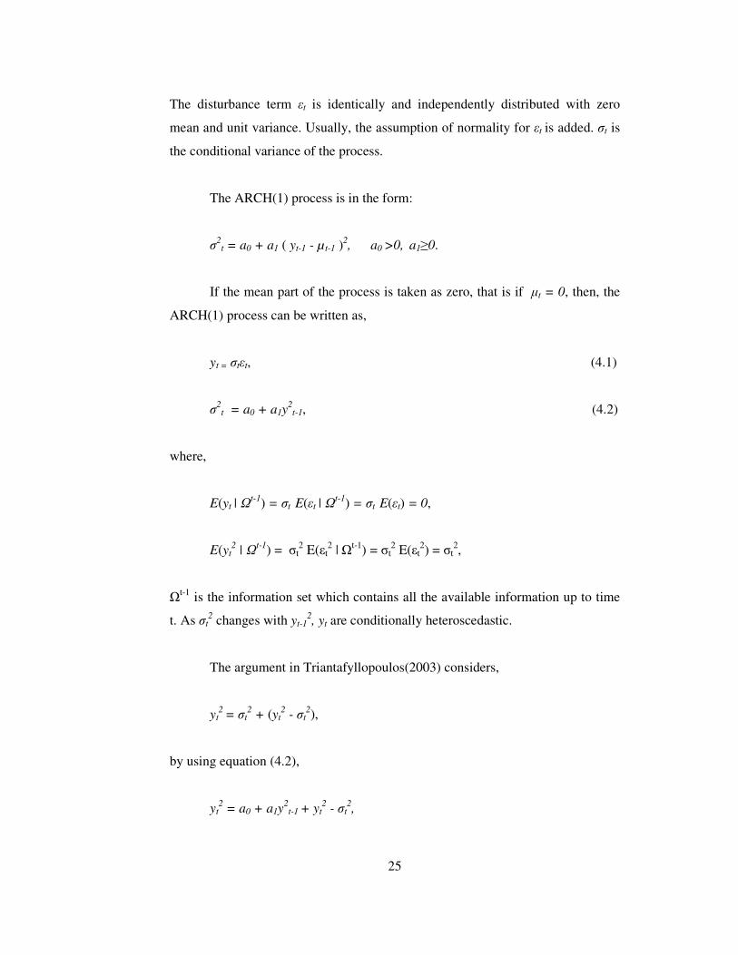
The disturbance term �t is identically and independently distributed with zero

mean and unit variance. Usually, the assumption of normality for �t is added. �t is

the conditional variance of the process.

The ARCH(1) process is in the form:

�2t = a0 + a1 ( yt-1 - µ t-1 )2, a0 >0, a1�0.

If the mean part of the process is taken as zero, that is if �t = 0, then, the

ARCH(1) process can be written as,

yt = �t�t, (4.1)

�2t = a0 + a1y2

t-1, (4.2)

where,

E(yt | �t-1) = �t E(�t | �t-1) = �t E(�t) = 0,

E(yt2 | �t-1) = �t

2 E(�t2 | �t-1) = �t

2 E(�t2) = �t

2,

�t-1 is the information set which contains all the available information up to time

t. As �t2 changes with yt-1

2, yt are conditionally heteroscedastic.

The argument in Triantafyllopoulos(2003) considers,

yt2 = �t

2 + (yt2 - �t

2),

by using equation (4.2),

yt2 = a0 + a1y2

t-1 + yt2 - �t

2,

26

yt2 = a0 + a1y2

t-1 + �t2 (�t2-1),

yt2 = a0 + a1y2

t-1 + vt,

where vt = �t2 (�t2-1).

The process yt2 as defined above follows a non-normal AR(1) model with the

innovations �t2 (�t2-1).

By the law of iterated expectation, E(yt) = E[E(yt|�-1)], and var(yt) =

E(�t2) = a0 + a1 var(y2

t-1). If a1<1, the process is stationary and var(yt) = a0/(1-a1).

Assuming that yt are conditionally normally distributed, E(yt4|�t-1) = 3�t

4 so that,

E(yt4) = 3E(a0

2 + 2a0a1yt-12 + a1

2yt-14),

=3(a02 + 2a0 a1 Var(yt-1

2) + a12 E(yt-1

4)).

When E(yt4) is constant,

m4 = [3a02(1 + a1)] / [(1-a1)(1-3a1

2)].

This implies that 0�a12�1/3. The kurtosis coefficient of yt is then,

m4 / var(yt)2 = 3(1-a12) / (1-3a1

2) > 3.

According to this result, it can be noted that the unconditional distribution of yt is

leptokurtic. That means, even yt are conditionally normally distributed, the

resulting ARCH(1) process can not be normal (Kuan, 2003).

An ARCH(1) process is easily generalized to an ARCH(q) process such

that,

27

yt = �t�t,

,1

20

2 �=

−+=q

iitit yaaσ

where a0>0, ai�0 (i = 1,… ,q). For stability of the process, a1 + a2+… + aq should

be less than one ( Li, Ling, McAleer, 2002).

Similar to ARCH(1) model, ARCH(q) model can be represented by an AR

representation with order q.

In order to test whether there exists an ARCH effect, a simple test can be

used. First step of the procedure is running a linear regression with explanatory

variables. Then, squared residuals of the regression are regressed on their q lags

such that �t2 = �0 + �1�t-12 + ....�p�t-q2 + vt and the R2 of the regression equation is

multiplied by the number of usable observation, T. The test statistic TR2 is

distributed as chi-square with degree of freedom q which is the number of

restriction on the null hypothesis �1 = �2 = .... �q = 0 . If the test value is greater

than the critical value the conditional variance has to be modelled, otherwise there

is no need for ARCH models (Engle, 1982).

There are some problems with ARCH(q) models. The required value of q

might be very large and the non-negativity constraints on coefficients might be

violated. Because of these reasons, Generalized Autoregreesive Conditionally

Heteroscedastic (GARCH) models are introduced.

4.2 Generalized Autoregressive Conditionally Heteroscedastic Models

Generalized Autoregressive Conditionally Heteroscedastic (GARCH)

models are first introduced by Bollerslev in 1986.

The standard GARCH(1,1) process is specified as:

28

yt = �t�t,

�2t = a0 + �1y2

t-1 + b1 �t-12, a0>0, a1, b1�0.

The conditional variance equation of GARCH(1,1) model contains a

constant term, news about volatility from the previous period, measured as the lag

of previous term squared residual �t-12 (the ARCH term), and last period’s forecast

variance �t-12 ( the GARCH term).

The unconditional mean and variance of GARCH(1,1) process can be

obtained by using law of iterative expectations such that,

E(yt) = E[E(yt|�-1)] = 0,

var(yt) = E(�t2) = a0 + a1 E(yt-1

2) + b1E(�t-12).

weak stationarity implies that

var(yt) = a0 / (1-a1-b1).

Thus, a1 + b1 must be less than one to variance be finite.

As in the ARCH process, in GARCH(1,1) model the marginal distribution

of yt is leptokurtic even if the conditional distribution is normal (Kuan, 2003).

As illustrated in Enders (1995), the more general GARCH(p,q) model is,

yt = �t�t,,

.1

2

1

20

2 ��=

−=

− ++=p

jjtj

q

iitit byaa σσ

29

It can be shown that any GARCH(p,q) process can be written in an

ARMA(p,q) representation (Kuan, 2003).

As stated by Peters (2001), the GARCH type models are estimated by

using a maximum likelihood (ML) approach. First, the conditional distribution of

yt has to be specified. The standard approach is to use conditional normal density.

However, as it is shown in chapter 4.1, the marginal distribution of yt will be

leptokurtic even if the conditional distribution is normal because financial time

series usually have excess kurtosis and skewness. Bollerslev and Wooldridge

(1992) introduce the quasi-maximum likelihood (QML) estimation method which

is robust to departures from normality. It was illustrated in Kuan (2003) that the

QMLE’s are asymptotically efficient if the conditional means and variances are

correctly specified.

As an alternative to conditional normal distribution, Bollerslev (1987),

and Kaiser (1996) use Student–t distribution while Nelson (1991), Kaiser (1996)

suggest Generalised Error Distribution (GED). On the other hand, Fernandez and

Steel (1998) use Skewed Student-t distribution.

In this study, the assumption of conditional normality is used in

estimation.

4.3 GARCH in Mean Models

In some financial applications, the expected return on an asset related to

the expected asset risk . For such cases Engle, Lilien and Robins (1987) suggest

GARCH in mean [GARCH-M] process. In these types of models, the mean of the

sequence depends on its own conditional variance such that,

yt = c + ��t2 + ut,

with ut = �t�t and

30

�2t = a0 + a1y2

t-1 + b1 �t-12, a0>0, a1, b1�0

In estimation of these models, ML estimation method is used like in GARCH

models.

4.4 Exponential GARCH Models

In GARCH models, due to the presence of yt2 in the variance equation, the

positive and negative values of the lagged innovations have the same effect on the

conditional variance. However, volatility responds to positive and negative shocks

differently, so in the case of volatility asymmetry GARCH models are not good

choices (Kuan, 2003). For this reason, exponential GARCH (EGARCH) models

were introduced by Nelson in 1991.

A simple EGARCH(1,1) model is,

yt = �t�t,

with conditional variance,

�t2 = exp [�+� ln(�t-1

2) +(yt-t /�t-1) + �| yt-t /�t-1| ].

In EGARCH process positive and negative shocks of the same magnitude

do not have the same effect on volatility and due to the exponential function, a

larger innovation has a larger effect on �t2. These are the basic differences

between GARCH and EGARCH models.

EGARCH(1,1) process can be extended to EGARCH(p,q) process such

that,

yt = �t � t,

31

.)ln(exp1 1

20

2

��

�

�

��

�

�

��

��

�

+++= � �

= = −

−

−

−−

q

i

p

j jt

jtj

jt

jtjitit

h

y

h

yγθσβασ

ARCH type models are the first attempts to deal with the volatility. They

have applied a lot so there are many references in the literature. The main

advantage is that they are easy to use models and the estimation is fast. However,

volatility modelling is very difficult because of uncertain events and ARCH type

models may not capture these surprises. When there are smooth changes the

performance of these models is good but when the changes are unexpected they

struggle. All ARCH/GARCH models are deterministic, that means they model the

volatility as a deterministic function. In order to be more realistic, the models

which consider the volatility stochastically should be considered.

4.5 Stochastic Volatility

The stochastic volatility (SV) model is an important alternative to the

ARCH type models and has attracted much attention recently. In ARCH /

GARCH models, the volatility is considered as deterministic however, in SV

models it is modelled as stochastic. That means SV considers the shocks affecting

volatility in contrast to GARCH but the main disadvantage of SV models is the

difficulty of estimation.

As illustrated in Kuan(2003), a simple SV process is,

yt = �t�t, (4.3)

ln(�t2) = �0 + �1 ln(�t-1

2) + vt, (4.4)

where |�1| <1 to ensure stationarity of ln(�t2). The volatility equation has

innovation term vt which is independent of �t. The inclusion of new innovations

32

makes the model more flexible but estimation of the process becomes much more

difficult.

If the assumption of normality is added, that is if �t ~ N(0,1) and vt ~

N(0,�v2), then,

E(ln�t2) = �0 + �1 E[ln(�t-1

2)] + E(vt),

Since |�1| <1 and vt has zero mean the expectation becomes,

E(ln�t2) = �0 / (1-�1).

To calculate the variance,

var(ln�t2) = �1

2 var[ln(�t-1

2)] + var(vt),

Again from stationarity of the process the variance is,

var(ln�t2) = �v

2/(1-�12).

That means ln�t2 is distributed as Normal with mean �0 / (1-�1) and variance

�v2/(1-�1

2).

If ln�t2 is distributed as normal then �t

2 is distributed as log-normal and the log-

normal distribution can be specified in terms of the parameters of normal

distribution. It is shown that,

ln�t2 ~ N {�0 / (1-�1) ,�v

2/(1-�12)},

then,

33

�t2 ~ log-normal {exp [�0 / (1-�1) + �v

2/2(1-�12)], exp [2 �0 / (1-�1)+ �v

2/(1-

�12)] exp [(�v

2/(1-�12)) -1]}.

Knowing that E(yt) = 0 and using above information the higher order

moments of yt can be calculated:

E(yt2)=E(�t

2)E(�t2) = exp [�0 / (1-�1) + �v2/2(1-�1

2)],

E(yt4) = E(�t

4)E(�t4) = 3 exp [2 �0 / (1-�1) + 2 �v2/ (1-�1

2)].

When the kurtosis of yt, m4, is calculated,

m4 = E(yt4) / [E(yt

2)]2 = 3 exp [�v2/ (1-�1

2)] > 3,

thus, yt is also leptokurtic.

An alternative and more commonly used representation of SV models are

given in Kim, Shephard and Chib (1998) such that,

yt = � eht/2 �t,

ht = � + (ht-1 – �) + ���t,

where the log-volatility is denoted by ht such that, ht = ln(�t2). The log-volatility

follows a stationary process if |�| < 1. �t and �t are uncorrelated standard normal

white noise shocks and �� is the volatility of the log-volatility. The parameter � or

exp (�/2) is constant scaling factor and in some cases � is taken as 0 so � will be

1.

34

4.5.1 SV Estimation

Unlike the ARCH/GARCH models, a SV model include error terms in

both mean and variance equations. The likelihood function is difficult to evaluate

and several methods have been developed to solve this estimation problem. Such

methods include generalized method of moments (GMM), quasi-maximum

likelihood (QML) estimation, Monte Carlo Markov chain (MCMC) methods. In a

Monte Carlo study, Andersen, Chung and Sorensen (1999) compared the

performances of various procedures and the MCMC method is found to be the

most efficient tool in making inferences about SV models. Therefore, in this

study, MCMC approach is used to estimate the parameters of the basic SV model.

Since MCMC is a Bayesian approach the basic ideas in Bayesian analysis

will be described below.

4.5.2 Bayesian Theory

As explained in Koop (2003), Bayesian econometrics is based on a few

simple rules of probability. For two random variables A and B, it is known that,

)(

)()|()|(

ApBpBAp

ABp = .

Similarly,

)()()|(

)|(yp

pypyp

θθθ = ,

where y is the data set and contains the unknown parameters. Bayesians treats

the as a random variable and p(|y) is the fundamental of interest. It gives all the

information about the parameters after observing the data. Ignoring p(y),

35

)()|()|( θθθ pypyp ∝

The term p(|y) is referred to as the posterior density, p(y|) is the likelihood

function and p() is the prior density.

If the mean of the posterior density, called posterior mean, is wanted to be

estimated,

E(|y) = � p(|y) d.

If g() is of interest rather than , then

E[g()|y]) = �g() p(|y) d.

In general, the above integral can not be evaluated analytically. Usually a

numerical method is needed and in Bayesian econometrics this method is called

as posterior simulation.

The simplest posterior simulator is referred as Monte Carlo integration.

The Monte Carlo integration has following steps:

Step1: Take a random draw, s from the posterior of .

Step2: Calculate g(s), where g(.) is a function of interest, keep the result.

Step3: Repeat step 1 and 2 S times.

Step 4: Take the average of the S draws of g(1),… , g(s). The average

value converges to E[g()|y] as S goes to infinity.

These steps give an estimate of E[g()|y] for any function g(.).

36

Monte Carlo integration is only an approximation. However, the degree of

approximation error can be controlled by selecting S. From central limit theorem

as S goes to infinity,

),0()}|))((ˆ{ 2gS NygEgS σϑ →− ,

where �g2 = var[g()|y] and it can be estimated by Monte Carlo integration. The

estimate is denoted as 2ˆ gσ . The confidence interval found by using normal

distribution for Sg , or the numerical standard error defined by Sgσ

can show the

accuracy of the estimation. If S = 10 000, for example, then the numerical

standard error is 1% as big as the posterior standard deviation.

In many cases, it is not possible to take random draws from p(|y) because

of the functional forms. However, dividing the parameter space into various

blocks such that = ((1), (2), ... (B)) and then taking random samples from full

conditional distributions p((1) | y, (2),...,(B)),… , p((B) | y, (1),..., (B-1)) is a

possible way. This approach is called as Gibbs sampler and it is a powerful tool

for posterior simulation. In this method, first an initial value is chosen and then

random draws of (i) conditional on previous draws are taken sequentially. It

yields a sequence of draws from the posterior. A possible problem in this

application is to select the initial value. However, the initial values do not matter

in the sense that the Gibbs sampler will give a sequence of draws from the

posterior and it is repeated S times. The first S0 of these replications are called as

burn- in replications and the remaining S1 is used in estimation. Generally, the

steps of the Gibss sampler as follows:

Step 0: Choose a starting value, (0), for s = 1,..., S

Step 1: Take a random draw, (1)(s) from p((1) |y, (2)

(s-1), ..., (B)(s-1)),

Step 2: Take a random draw, (2)(s) from p((2) |y, (1)

(s-1),..., (B)(s-1)),

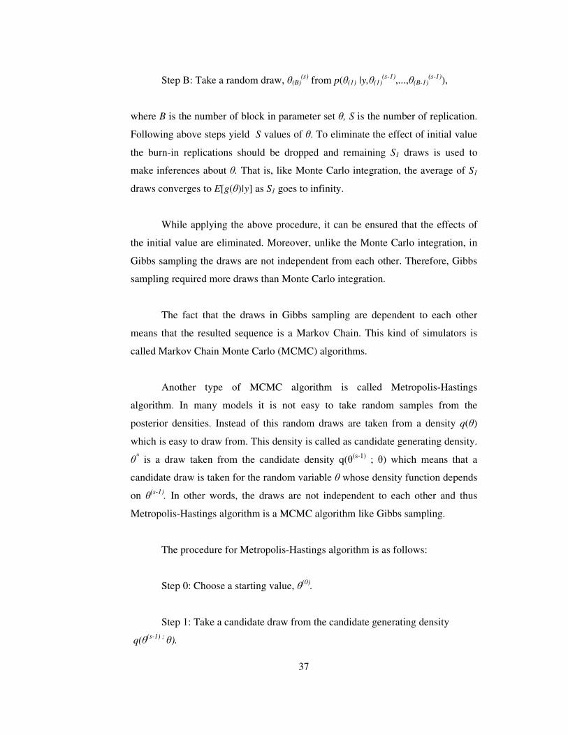
37

Step B: Take a random draw, (B)(s) from p((1) |y,(1)

(s-1),...,(B-1)(s-1)),

where B is the number of block in parameter set , S is the number of replication.

Following above steps yield S values of . To eliminate the effect of initial value

the burn-in replications should be dropped and remaining S1 draws is used to

make inferences about . That is, like Monte Carlo integration, the average of S1

draws converges to E[g()|y] as S1 goes to infinity.

While applying the above procedure, it can be ensured that the effects of

the initial value are eliminated. Moreover, unlike the Monte Carlo integration, in

Gibbs sampling the draws are not independent from each other. Therefore, Gibbs

sampling required more draws than Monte Carlo integration.

The fact that the draws in Gibbs sampling are dependent to each other

means that the resulted sequence is a Markov Chain. This kind of simulators is

called Markov Chain Monte Carlo (MCMC) algorithms.

Another type of MCMC algorithm is called Metropolis-Hastings

algorithm. In many models it is not easy to take random samples from the

posterior densities. Instead of this random draws are taken from a density q()

which is easy to draw from. This density is called as candidate generating density.

* is a draw taken from the candidate density q((s-1) ; ) which means that a

candidate draw is taken for the random variable whose density function depends

on (s-1). In other words, the draws are not independent to each other and thus

Metropolis-Hastings algorithm is a MCMC algorithm like Gibbs sampling.

The procedure for Metropolis-Hastings algorithm is as follows:

Step 0: Choose a starting value, (0).

Step 1: Take a candidate draw from the candidate generating density

q((s-1) ; ).

38

Step 2: Calculate an acceptance probability, �((s-1), *).

Step 3: Set (s) = * with probability �((s-1), *) and set (s) = (s-1) with

probability 1- �((s-1), *).

Step 4: Repeat steps 1, 2, 3 S times

Step 5. Take the average of the S draws g((1)),… , g((S)).

These steps give an estimate of E[g()|y]. The difference in Metropolis-Hastings

algorithm is not all the draws are accepted. There is an acceptance probability

such that:

((s-1), *) = ��

���

�

====

−−

−

1,);()|(

);()|(min *)1()1(

)1(**

θθθθθθθθθθ

ss

s

qypqyp

,

where p( = *|y) is the posterior density at point *, q( *; ) is a density for

and so q( *; = (s-1)) is the density for evaluated at (s-1).

In some cases, some conditional posterior distributions are easy to draw

from but one or two conditionals do not have a convenient form. In these types of

situations Metropolis-within-Gibbs algorithms are commonly used. Gibbs

sampling is applied to the conditional posteriors which have easy form and

Metropolis-Hastings algorithm is used for the other ones.

4.5.3 MCMC for SV

In a basic SV model which is represented by equations (4.3) and (4.4) the

parameters are =(, � �2, µ). The posterior of can be written as:

).()|()|( θθθπ fyfy ∞

39

where f(y|) is the likelihood function and f() is the prior density for . However,

since,

�= dhhfhyfyf )|(),|()|( θθθ ,

(where h = (h1,… ,hT) is the T volatilities) is difficult to find, and so the direct

analysis of )|( yθπ is not possible. In such cases, posterior simulators can be

used. A possible way to solve this problem is to apply Gibbs sampling which is a

MCMC algorithm. In Gibbs sampling, as explained before, the parameter space is

divided into blocks and the algorithm proceeds by sampling each block from the

full conditional distributions. One cycle of the algorithm is called sweep or a scan,

the draws from the sampler will converge to the draws from the density in interest

as the number of sweeps increases.

For the basic SV model, the parameter space is (,h) where =(, � �2, µ).

The Gibbs sampling algorithm for the SV model is given in Kim, Shephard and

Chip (1998) as follows:

1. Initialize h and .

2. Sample ht from h-t, y, � , t=1,…,T (h-t denotes the rest of the h vector

other than ht).

3. Sample � �2| y, h, , µ,

4. Sample | y, h, µ, � �2,

5. Sample µ| y,h,, � �2.

6. Go to 2.

40

Cycling from 2 to 5 is a complete sweep of this sampler. Many sweeps

should be performed to generate samples from , h| y.

The most difficult part of the algorithm is to sample from ht| h-t, yt, since

this operation has to be done T times for each sweep. However, in SV models it is

not possible to sample directly from f(ht| h-t, yt, ) because

),|(),|(),,|( θθθ ttttttt hyfhhfyhhf −− ∝ t=1,...,n

so Metropolis-Hastings procedure is used to draw from f(ht| h-t, yt, ). The

candidate density is taken as normal with parameters �t, vt2

To get ��2 random draws from inverse-gamma distribution are taken such

that,

���

���

�

���

���

� −−−+−−++ �

−

=+

2

))()(()1()(,

2~

1

1

21

221

2

n

ttt

r

hhhSn

IGµϕµϕµ

σσσ

η ,

where 5=rσ , and rS σσ ×= 01.0 .

Metropolis-Hastings procedure is used for sampling � and the candidate

distribution is assumed to be normal with parameters ϕ and ϕV .

Finally, again normal distribution is used for drawing samples of µ such

that,

),ˆ(~ 2µσµµ N

All of the parameters mentioned above are stated explicitly by Kim,

Shephard and Chip (1998).

41

This algorithm is done by an Ox code which is fully documented in the

web site http://www.nuff.ox.ac.uk/users/shephard/ox/ (3 May 2004). This

program calculates the estimated values of the parameters and log-likelihood ratio

statistics of SV model automatically.

42

CHAPTER 5

APPLICATION OF VOLATILITY MODELS ON TURKISH FINANCIAL

DATA

In order to illustrate the volatility models, the weekly observations on

Turkish T.L/ USA $ exchange rates from the first week of October 1989 until the

last week of the December 2003 are taken.

The graph of the data is shown in Figure 5.1,

6

8

10

12

14

16

100 200 300 400 500 600 700

LNDOLLAR

Figure 5.1: Plot of the TL/Dollar exchange rates

It is easily seen that the series contains a trend component which should be

removed before modelling. To remove the trend first we should decide whether it

is deterministic or stochastic. In order to do this ADF unit root test is applied two

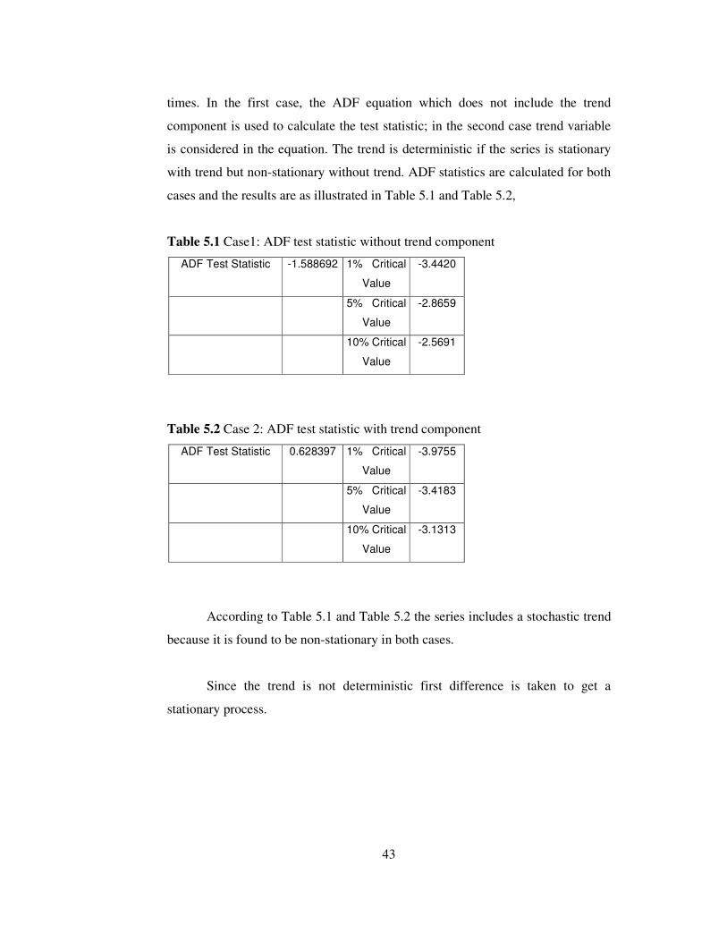
43

times. In the first case, the ADF equation which does not include the trend

component is used to calculate the test statistic; in the second case trend variable

is considered in the equation. The trend is deterministic if the series is stationary

with trend but non-stationary without trend. ADF statistics are calculated for both

cases and the results are as illustrated in Table 5.1 and Table 5.2,

Table 5.1 Case1: ADF test statistic without trend component

ADF Test Statistic -1.588692 1% Critical

Value

-3.4420

5% Critical

Value

-2.8659

10% Critical

Value

-2.5691

Table 5.2 Case 2: ADF test statistic with trend component

ADF Test Statistic 0.628397 1% Critical

Value

-3.9755

5% Critical

Value

-3.4183

10% Critical

Value

-3.1313

According to Table 5.1 and Table 5.2 the series includes a stochastic trend

because it is found to be non-stationary in both cases.

Since the trend is not deterministic first difference is taken to get a

stationary process.

44

-6

-4

-2

0

2

4

6

8

100 200 300 400 500 600 700

RET URN

Figure 5.2: Plot of the difference of the TL/Dollar exchange rates

Figure 5.2 shows the plot of the first difference, and it suggests that a time-

varying volatility and volatility clustering is quite evident in the data. From the

plot, the differenced series is stationary. However, to test statistically again ADF

unit root test applied.

Table 5.3 Unit root test for difference of TL/Dollar exchange rates

ADF Test Statistic -13.73746 1% Critical

Value*

-3.4420

5% Critical

Value

-2.8659

10% Critical

Value

-2.5691

According to Table 5.3, the ADF test statistics is greater than all the

critical values in absolute value so the hypothesis of non-stationarity is rejected.

That means the differenced series is stationary which is denoted as I(0).

In financial time series analysis, the log value of the first differenced series

is called as the return and in practice mean- corrected returns are mainly dealing

with such that,

45

.)log(log1

)log(log1001

11���

��� −−−×= �

=−−

n

iiittt rr

nrry

where rt denotes the exchange rate at time t. Therefore, the percentage mean-

corrected returns are calculated for the TL/Dollar exchange rates and the resulting

series yields the basic statistics values as in Figure 5.3.

Figure 5.3 Descriptive statistics for the TL/Dollar exchange rates

As it is seen in Figure 5.3 that, the kurtosis value is high which supports

the claim that many financial time series have a leptokurtic distribution and also

from the Jarque-Bera test, the hypothesis of normality is strongly rejected.

In practice, while dealing with volatility the mean part of the process is not

taken into account and the variance is modelled only. Therefore, µ t is taken as

zero when applying volatility models.

Before modelling the variance the squared of the residuals, in this case the

data itself, should be checked whether they include any ARCH effects or not. In

order to test whether there exists any ARCH effects or not, the ARCH-LM test is

applied to the data.

0

50

100

150

200

-4 -2 0 2 4 6

Series: RETURN Observations 721 Mean -0.101773 Median -0.084155 Maximum 7.230558 Minimum -5.467083 Std. Dev. 1.267858 Skewness 0.520096 Kurtosis 7.650156 Jarque-Bera 682.1244 Probability 0.000001

46

Table 5.4 Test results of autocorrelation

H0: no autocorrelation in squared returns

Lag F value p value

1 82.959930. 0.000001

up to 2 43.18155 0.000001

up to 3 34.48939 0.000001

up to 30 5.745111 0.000001

According to Table 5.3 the hypothesis of no autocorrelation in squared

returns is rejected at all lags therefore the volatility should be modelled by either

an ARCH type or a stochastic model.

5.1.Estimation of GARCH models

Various deterministic volatility models are fitted to the data. Actually, in

practice higher order GARCH models are not preferred because it is known that

GARCH(1,1) is able to capture the variance changing as well as the higher order

ARCH type models so GARCH(1,1), E-GARCH and M-GARCH models are

fitted to the data. The results are given in Table 5.5, Table 5.6 and Table 5.7,

respectively.

47

Table 5.5 GARCH(1,1) results for percentage return

Dependent Variable: RETURN

Method: ML - ARCH

Date: 08/11/04 Time: 17:22

Sample: 1 721

Included observations: 721

Convergence achieved after 20 iterations

Coefficient Std. Error z-Statistic Prob.

Variance Equation

C 0.064891 0.013004 4.990052 0.0001

ARCH(1) 0.243420 0.037571 6.478876 0.0001

GARCH(1) 0.734854 0.033985 21.62267 0.0001

R-squared -0.006453 Mean dependent var -0.101773

Adjusted R-squared -0.009256 S.D. dependent var 1.267858

S.E. of regression 1.273712 Akaike info criterion 2.894291

Sum squared resid 1164.842 Schwarz criterion 2.913351

Log likelihood -1040.392 Durbin-Watson stat 1.182303

Table 5.6 E-GARCH(1,1) results for percentage return

Dependent Variable: RETURN

Method: ML - ARCH

Date: 08/11/04 Time: 17:23

Sample: 1 721

Included observations: 721

Convergence achieved after 39 iterations

Coefficient Std. Error z-Statistic Prob.

Variance Equation

C -0.312529 0.034133 -9.156203 0.0001

|RES|/SQR[GARCH](1) 0.422061 0.047251 8.932262 0.0001

RES/SQR[GARCH](1) 0.024757 0.014344 1.725998 0.0843

EGARCH(1) 0.940813 0.013651 68.91974 0.0000

R-squared -0.006453 Mean dependent var -0.101773

Adjusted R-squared -0.010664 S.D. dependent var 1.267858

S.E. of regression 1.274600 Akaike info criterion 2.893941

Sum squared resid 1164.842 Schwarz criterion 2.919354

Log likelihood -1039.266 Durbin-Watson stat 1.182303

48

Table 5.7 M-GARCH(1,1) results for percentage return

Dependent Variable: RETURN

Method: ML - ARCH

Date: 08/11/04 Time: 17:25

Sample: 1 721

Included observations: 721

Convergence achieved after 23 iterations

Coefficient Std. Error z-Statistic Prob.

GARCH -0.051835 0.025990 -1.994449 0.0461

Variance Equation

C 0.068398 0.013665 5.005343 0.0001

ARCH(1) 0.253028 0.037704 6.710844 0.0001

GARCH(1) 0.723407 0.033582 21.54171 0.0001

R-squared -0.004405 Mean dependent var -0.101773

Adjusted R-squared -0.008607 S.D. dependent var 1.267858

S.E. of regression 1.273303 Akaike info criterion 2.894733

Sum squared resid 1162.473 Schwarz criterion 2.920146

Log likelihood -1039.551 Durbin-Watson stat 1.168448

Comparing different GARCH type models by looking at AIC and SBC, M-

GARCH models with both variance and standard deviation term in the mean

equation are not preferred. If the E-GARCH and GARCH(1,1) models are

anlaysed, AIC of E-GARCH and SBC of GARCH(1,1) is smaller. However, SBC

has better properties and it is more commonly used in comparison than AIC(

Enders, 2003) so GARCH(1,1) is chosen between the deterministic type of

volatility models.

Error terms may be checked after deciding the suitable model. Descriptive

statistics are obtained and shown in Figure 5.4. According to them, the

distribution of the error term is not normal, it is leptokurtic and the Jarque-Bera

test also rejects the normality which does not conflict with the theory.

49

Figure 5.4 Descriptive statistics for the error term under GARCH(1,1) process

As a result the following GARCH(1,1) process is fitted to the data in order

to model the volatility.

yt = �t�t,,

�2

t = 0.064891 + 0.243420y2t-1 + 0.734854 �t-1

2.

The parameters should satisfy the stationarity conditions in the conditional

variance equation. The sum of 0.243420 + 0.734854 = 0.978274 < 1 and all

coefficients are positive that means the restrictions are satisfied for the

GARCH(1,1) model.

5.2 Estimation of SV model

As explained before, the GARCH types models consider the variance of

the series as deterministic although it can be stochastic. Therefore the following

SV model is estimated:

0

40

80

120

160

-2 0 2 4 6

Series: Standardized Residuals Sample 1 721 Observations 721

Mean -0.012620 Median -0.034912 Maximum 7.429422 Minimum -2.977934 Std. Dev. 0.999175 Skewness 0.840634 Kurtosis 7.850459

Jarque-Bera 791.7064 Probability 0.000001

50

yt = � eht/2 �t,

ht = � + � (ht-1 – �) + ���t,

where �t and �t are uncorrelated white noise processes.

In order to estimate the SV model an MCMC algorithm is used which is

completely done by the written Ox code. The MCMC sampler was initialized by

setting all the ht = 0, and � = 0.95, � �2 = 0.02 and µ = 0. The algorithm is

iterated 50,000 times. The burn-in period is large enough to ensure that the effect

of the starting values becomes insignificant. The results are summarized in Table

5.8.

Table 5.8 Estimation results for the SV model

Parameter mean MC STD Error Inefficiency

�|y 0.97059 0.00083224 19.723

��|y 0.26768 0.0053653 70.699

�=exp(µ/2)|y 0.94034 0.0047216 2.2324

According to the results, � is very close to the one, that means the shocks

in the log-variance are highly persistent as in the case of the GARCH. The

numerical standard errors of the sample mean deriving from the Monte Carlo

simulation are considered as a measure of the accuracy of the estimates. The

accuracy could be improved by increasing the number of iterations. The

simulation inefficiency factors measure how well the Markov Chains mixes. It is

defined as the ratio of the numerical variance (i.e. square of the Monte Carlo

standard error) and the variance of the sample mean that would derive from

drawing independent samples, as independent random draws would be the optimal

outcome of the simulation procedure, the most desirable inefficiency factor is one

that closest to one. The inefficiency factor can be interpreted as the number of

51

times the algorithm needs to be run to produce the same accuracy in the estimate

that would derive from independent draws. The inefficiency factor can generally

be reduced by increasing number of iterations (Pederzoli, 2003).

After fitted the SV model to the data the diagnostic checks can be applied

to the error term.

Figure 5.5 Descriptive statistics for the error term under SV process

Figure 5.5 shows that the resulting error term has a high kurtosis value and

it is far from being normal. The normality is also rejected with the Jarque-Bera

test.

Two different types of volatility models are fitted to the data, now it

should be cleared that which type is more suitable to the percentage returns. In

order to compare the GARCH and SV models, the likelihood ratio test statistic

will be used.

5.3 Comparison of GARCH and SV

In order to compare the SV and GARCH (1, 1) models a hypothesis testing

procedure may be applied. Hypothesis testing theory is usually advocated when

0

40

80

120

160

-6 -4 -2 0 2 4 6 8

Series: ERROR Sample 1 721 Observations 721

Mean -0.108230 Median -0.089494 Maximum 7.689302 Minimum -5.813943 Std. Dev. 1.348298 Skewness 0.520096 Kurtosis 7.650155

Jarque-Bera 682.1243 Probability 0.000001

52

one of the hypotheses H0 can be considered as a limiting case of H1. That means,

the model shown H1 is reduced to the model in H0 by imposing some restrictions.

In these cases, H0 is said to be nested in H1 ( Gourieroux, 1994). However, in the

case of SV and GARCH models the usual nested hypothesis procedures can not

be applied because the models of interest are non-nested. A different procedure

will be used in order to decide which model is better to construct. In this study,

the likelihood ratio test statistics which relies on simulation suggested by

Atkinson (1986) is calculated to test the hypothesis.

The likelihood ratio (LR) test statistic for comparing the models is given

by,

{ })ˆ,|(log),|(log2 0011 θξθξ yfyfLR y −= ,

where 1ξ denotes the SV model and 0ξ the GARCH model and ),|(log 11 θξyf ,

)ˆ,|(log 00 θξyf denote the respective estimates of the log likelihoods. The

sampling variation of LRy under the SV model is true or under the alternative that

GARCH model is true is approximated by simulation. The procedure is as

follows:

Under the assumption of SV model is true, 999 set of yi values are

generated. For each simulated series, the parameters of GARCH and SV models

are estimated and then the value of LRyi ( i=1… 999) statistic is recorded. The

resulting values of LRy1,… ..LRy

999 are a sample from the exact distribution of LRy

under the SV null. After that, the empirical LRy value is ranked in the 999

simulated LRyi values. If it is the largest, H0 is rejected at 0.1% significance level;

if it is 23th, the significance level is 2.3% and if it is 437, for example, there is no

evidence against the SV model.

For TL/Dollar exchange rates the log-likelihood ratio statistics for the

GARCH (1,1) model is -1040.392 and for SV model it is calculated as -1022.2 .

53

For testing the GARCH versus the alternative of SV, LR test statistics can be

calculated as,

LRy= 2{ -1022.2+1040.392} = 36.384.

When the data are simulated from the GARCH model with estimated

paramaters and when the value of the LR statistics is compared with the 999

simulated values, it is found that all of the LR values are negative while the

empirical value is positive, that is the LRy is the largest among the simulated

values and so GARCH model is rejected at 0.1% level.

The same procedure is applied to test the null hypothesis of SV model

against the alternative of GARCH(1,1) model. This time, data are generated from

the SV model and again 999 simulated LR values are obtained by using artifical

observations. According to the results, the empirical value of 36.384 is smaller

than all of the simulated LR test statistics so the hypothesis of SV model does not

rejected with probability 0.999. Therefore, both tests are consistent with each

other and this implies that SV model is a beter alternative than the GARCH(1,1)

model. In other words, the non-nested LR test statistics give strong evidence

against the use of GARCH(1,1) model for the case of TL/Dollar exchange rate

data,which implies that modelling volatility as stochastic rather than deterministic

will be better.

54

CHAPTER 6

CONCLUSION

Volatility is a key variable which plays a central role in many areas of

finance, most of the financial data have heteroscedasticity problem and exhibit

volatility clustering therefore it is important to model volatility correctly. In this

study, firstly a brief introduction to the volatility modeling is given. After that, the

most commonly used models for volatility are covered. A simple ARCH model

and its extensions, namely GARCH, GARCH-M and EGARCH models are

explained as non-stochastic variance models. Following the ARCH type models,

the SV process which models the volatility stochastically is considered. In order

to compare them, the parameters of both type models are estimated. The

estimation procedures of two kinds of models are different from each other. In

ARCH type models, QMLE is used in estimation. It is easy to apply and robust to

departures from normality. On the other hand, in SV case a Bayesian approach is

considered to estimate the model. The MCMC method, namely the Metropolis-

Hastings and Gibbs sampling algorithms, is used since it is found to be the most

efficient way to estimate the SV model.

In the application part, the weekly exchange rates of Turkey / USA are

analyzed. The mean part is not taken as important since the main aim is to model

the volatility. Among other non-stochastic processes, the GARCH (1,1) model is

decided to be the most appropriate for the time-varying variance of the data. The

estimators of GARCH (1,1) model are obtained by the help of the package E-

55

views 3.0. The procedure is fast and easy to do. After that, SV model is estimated

by applying the MCMC procedure which is done by an Ox code.

In order to decide which model is better, first the null hypothesis of

GARCH(1,1) is tested versus the alternative of SV model. The log-likelihood

ratio (LR) test statistics calculated for non-nested models. The empirical value of

the LR test statistics is obtained by using the relevant formula and it is found to be

36.384. After that, the data is generated artificially from the GARCH(1,1) and SV

models respectively to get the simulated LR values. By comparing the empirical

value with the simulated ones, the empirical value is found to be the largest and

so GARCH(1,1) model is rejected at 0.1% level. In the second case, the null

hypothesis of SV model is tested versus the alternative of GARCH(1,1) model

and this time we do not reject the null hypothesis of SV according to the results of

the LR test statistics. That means, both test results support the claim that SV

model is a better choice than the GARCH(1,1) model. Therefore, for the case of

Turkish/ USA weekly exchange rate data, modeling volatility stochastically will

be better than considering it as non-stochastic depending on the results of LR test

statistics.

The basic SV model can be extended by taking the underlying distribution

as to be a more heavy-tailed than the normal distribution, for example the student-

t distribution, or the multivariate SV models may be estimated which can be a

future work relating with the topics of this thesis.

56

REFERENCES

Andersen, T. G. (1994). Stochastic autoregressive volatility: A framework for

volatility modelling. Mathematical Finance, 4, 75-102.

Andersen, T. G. and Sqrensen, B. (1993). GMM estimation of a Stochastic

volatility model: A Monte Carlo study. Discussion paper, Northwestern

University.

Atkinson, A. C. (1989). Monte-Carlo tests of separate families of hypotheses.

Unpublished paper, Imperial College, London.

Baillie, R. and Bollerslev, T. (1989). The message in daily exchange rates: A

conditional variance tale. Journal of Business and Economis Statistics, 7, 297-

305.

Bera, A. K. and Higgins, M. L. (1993). On ARCH models: properties, estimation

and testing. In L. Exley, D. A. R. George, C. J. Roberts and S. Sawyer (eds.),

Surveys in Econometrics.(Basil Blackwell: Oxford) Reprinted from Journal of

Economic Surveys.

Bodurtha, J. N. and Mark, N. (1991). Testing the CAPM with time varying risks

and returns. Journal of Finance, 46, 1485-1505.

Bollerslev, T. (1986). Generalized Autoregressive Conditional Heteroscedasticty.

Journal of Econometrics, 31, 307-327.

57

Bollerslev, T. (1987). A conditionally Hhteroskedastic time series model for

speculative prices and rates of return. Review of Economics and Statistics, 69,

542-547.

Bollerslev, T. (1990). Modelling the coherence in short-run nominal exchange

rates: A multivariate generalized ARCH approach. Review of Economics and

Statistics, 72, 498-505.

Bollerslev, T. , Chou, R.Y. and Kroner, F.K (1992).ARCH modelling in finance:

A review of the theory and emprical evidence. Journal of Econometrics, 52, 5-59.

Bollerslev, T., Engle, R. and Nelson, D. (1994). ARCH models. Handbook of

Econometrics, IV.

Bollerslev, T., Engle, R. and Wooldridge, J M. (1988). A capital asset pricing

model with time varying covariances. Journal of Political Economy, 96, 116-131.

Bollerslev, T. and Wooldridge, J. M. (1992). Quasi maximum likelihood

estimation and inference in dynamic models with time varying covariances.

Econometric Reviews, 11, 143-155.

Carter, C.K. and Kohn, R. (1994). On Gibbs sampling for state space models.

Biometrika, 81, 541-53.

Chib, S., Nardari, F. And Shephard, N. (2002). Markov chain Monte Carlo

methods for stochastic volatility models. Journal of Econometrics, 108, 281-316.

Cribari, F. (1997). Econometric programming environments GAUSS, OX and S-

PLUS. Journal of Applied Econometrics, 12, 77-89.

58

Dickey, D. A. and Fuller, W. A. (1979). Distribution of the estimators

autoregressive time series with a unit root. Journal of the American Statistical

Association, 74, 427-443.

Ding, Z., Granger, C. W. J. and Engle, R. F. (1993). A long memory property of

stock market returns and a new model. Journal of Empirical Finance, 1, 83-106.

Duan, J. (1997). Augmented GARCH(p,q) process and its diffusion limit. Journal

of Econometrics. 79(1), 97-127.

Duffie, D. and Singleton, K. J. (1993). Simulated moment estimation of Markov

models of asset prices, Econometrica, 61, 929-952.

Durbin, J. and Koopman, S.J. (1998). Time series analysis of non-Gaussian

observations based on state space models from both classical and Bayesian

perspectives. Journal of Royal Statistical Societyi Series B, 62, 3-56.

Enders, W. (1995). Applied Econometric Time Series. John Wiley and Sons, NY.

Engle, R. (1982). Autoregressive conditional heteroskedasticity with estimates of

the variance of United Kingdom inflation. Econometrica, 50, 987-1007.

Engle, R. (2002). New fronties for ARCH models. Journal of Applied

Econometrics, 17, 425-446.

Engle, R. and Bollerslev, T. (1986). Modelling the persistence of conditional

variances. Econometric Reviews, 5, 1-50.

Engle, R., Lilien, D. M. and Robins, R. P. (1987). Estimating time varying risk

premia in the term structure: The ARCH-M model. Econometrica, 55, 391-407.

59

Engle, R. F. and Ng, V. (1993). Measuring and testing the impact of news on

volatility. Journal of Finance, 48, 1747-1778.

Fama, E. F. (1965). The behaviour of stock market prices. Journal of Business,

38, 34-105.

Fernandez, C. and Steel, M. (1998). On Bayesian modeling of fat tails and

skewness. Journal of American Statistical Association, 93, 359-371.

Gallant, A.R. and Nychka, D. W. (1987). Seminonparametric maximum

likelihood estimation, Econometrica 55, 363-390.

Gallant, A. R., Rossi, P. E. and Tauchen, G. (1990). Stock prices and volume.

Unpublished manuscript (Department of Economics, Duke University, Durham,

NC).

Gamerman, D. (1997). Markov Chain Monte Carlo, Chapman & Hall, England.

Ghysels, E. and Harvey, A., Renault, E. (1995). Stochastic volatility. Handbook of

Statistics, 14.

Gilks, W. R., Richardson, S. and Spiegelhalter, D. J. (1996). Chapman & Hall,

England.

Glosten, L., Jagannathan, R. and Runkle, D. (1991). Relationship between the

expected value and the volatility of the nominal excess return on stocks.

Unpublished manuscript ( J.L. Kellogg Graduate Scholl, Northwestern University,

Evanston, IL).

Glosten, L., Jagannathan, R. and Runkle, D. (1993). On the relation between

expected return on stocks. Journal of Finance, 48, 1779-1801.

60

Gourieroux, C. (1994). Testing non-nested hypotheses. Handbook of

Econometrics, IV.

Goyal, A. (2000). Predictability of Stock return volatility from GARCH models.

Anderson Garduate School of Management, UCLA.

Gweke, J. (1986). Modelling persistence in conditional variances: A comment .

Econometric Reviews, 5, 57-61.

Gweke, J. (1988). Exact inference in models with autoregressive conditional

heteroskedasticity. in: E. Berndt, H. White and W. Barnett, eds., Dynamic

Econometric Modelling (Cambridge University Press, Cambridge) 73-104.

Hansen, P. R. and Lunde, A. (2003). A forecast comparison of volatility models:

Does anything beat a GARCH(1,1) model?. Unpublished paper.

Harvey, A. C. and Shephard, N. (1995). Estimation of testing of stochastic

variance models, Discussion paper, London School of Econometrics.

Harvey, A. C. , Ruiz, E. and Shephard, N. (1994). Multivariate stochastic variance

models. Review of Economic Studies, 61, 247-264.

Hentshel, L. (1995). All in the family: Nesting symmetric and asymmetric

GARCH models. Journal of Financial Economics, 39, 71-104.

Higgings, M. L. and Bera, A. K. (1992). A class of nonlinear ARCH models.

International Economic Review, 33, 137-158.

Hol, E. and Koopman, S.J. ( 2002). Stock index volatility forecasting with high

frequency data. Department of Accounting and Finance, Univeristy of

Birmingham, and Department of Econometrics, Free University Amsterdam,

Tinbergen Institude discussion paper.

61

Hsieh, D. (1989). Modelling heteroskedasticity in daily foreign exchange rates.

Journal of Business and Economic Statistics, 7, 307-317.

Jacquier, E., Polson, N. G. and Rossi, E. P. (1994). Bayesian analysis of stochastic

volatility models. Journal of Business and Economis Statistics, 12, No:4, 371-389.

Jacquier, E., Polson, N. G. and Rossi, E. P. (2002). Bayesian analysis of stochastic

volatility models with fat tails and correlated errors. Journal of Business and

Economic Statistics, 20, 69-87.

Jorion, P. (1988). On jump processes in the foreign exchange and stock markets.

The review of Financial Studies, 68, 165-176.

Kaiser, T. (1996). One-Factor-GARCH Models for German Stocks-Estimation

and Forecasting, University Tubingen, Working Paper.

Kim, S., Shephard, N. and Chib, S. (1998). Stochastic volatility: Likelihood

inference and comparison with ARCH models. Review of Economic Studies, 65,

361-393.

Koop, G. (2003). Bayesian Econometrics, John Wiley & Sons, England.

Koopman, S. J., Shephard, N. And Doornik, J. A. (1998). Statistical algorithms

for models in state space using SsfPack 2.2. Econometrics Journal, 2, 107-160.

Koopman, S. J. and Charles, B. ( 2000). Time series models with a common

stochastic variance component. Free University Amsterdam.

Koopman, S. J. and Uspensky, E. H. (2000). The stochastic volatility in mean

model. Tinbergen Institute, discussion paper.

62

Kuan, C. (2003). Lecture on basic time series models. Institute of Economics,

Academia Sinica, Lecture notes.

Lambert, P. and Laurent, S. (2000). Modelling skewness dynamics in series of

financial data. Discussion Paper, Institut de Statistique, Louvain-la-Neuve.

Liu, S. M. and Brorsen, B. (1995). Maximum likelihood estimation of a GARCH-

STABLE model. Journal of Applied Econometrics, 2.273-285.

Li, K. W., Ling, S. and McAleer, M. (2002). Recent theoretical results for time

series models with GARCH errors. Journal of Economic Survey, 16, 245-269.

Mark, N. (1988). Time varying betas and risk premia in the pricing of forward

foreign exchange contracts, Journal of Financial Economics, 22, 335-354.

Mahieu, J. R. and Schotman, P. C. (1998). An emprical application of stochastic

volatility models. Journal of Applied Econometrics, 13, 333-360.

Mandelbrot, B. B. (1963). The variation of certain speculative prices. Journal of

Business, 36, 394-416.

Melino, A. and Turnbull, M. (1990). Pricing foreign currency options with

stochastic volatility. Journal of Econometrics, 45, 239-265.

Nelson, D. (1991). Conditional heteroskedasticity in asset returns: a new

approach. Econometrica, 59, 349-370.

Pagan, A. R. and Ullah, A. (1988). The econometric analysing of models with rik

terms. Journal of Applied Econometrics, 3, 87-105.

63

Pantula, S. G. (1985). Estimation of autoregressive models with ARCH errors.

Unpublished manuscript, Department of Statistics, North Carolina State

University, Raleigh, NC).

Pantula, S. G. (1986). Modelling persistence in conditional variances A comment.

Econometric Reviews, 5, 71-74.

Pederzoli, C. (2003). Stochastic volatility and GARCH: A comparison based on

UK stock data. University of Warwick.

Peseran, M. H. and Peseran, B. (1990). Simulation approach to the problem of

computing Cox’ s statistic for testing nonnested models. Journal of Econometrics,

57, 377-392.

Peters, J. P. (2001). Estimating and forecasting volatility of stock indices using

asymmetric GARCH models and (Skewed) Student-t densities. Unpublished

paper, Université de Liége, Belgium.

Robinson, P. M. (1987). Testing for strong serial correlation and dynamic

conditional heteroskedasticity in multiple regression. Journal of Econometrics,

47, 67-84.

Ruiz, E. (1994). Quasi- maximum likelihood estimation of stochastic volatility

models. Journal of Econometrics, 63, 289-306

Sentana, E. (1995). Quadratic ARCH models. Review of Economic Studies, 62(4),

639-661.

Schwert, G. W. (1989). Why does stock volatility change over time? Journal of

Finance, 44(5), 1115-1153.

64

Simon, D. (1989). Expectations and risk in the treasury bill market: An

instrumental variable approach. Journal of Financial and Quantitative Analysis,

24, 357-366.

Taylor, S. J. (1986). Modelling Financial Time Series. John Wiley & Sons, NY.

Triantafyllopoulos, K. (2003). An introduction to stochastic volatility, University

of Newcastle, Lecture notes.

Türker, Ö. (1999). Structural Time Seires Modelling of Inflation Behaviour in

Turkey. Master Thesis, Department of Statistics, METU.

Vlaar, P. and Palm, F. (1993). The message in weekly exchange rates in the

european monetary system: mean reversion, conditional heteroskedasticity and

jumps. Journal of Business and Economic Statistics, 11, 351-360.

Whistler, D. (1988). Semi-parametric ARCH estimation of intra daily exchange

rate volatility. Unpublished manuscript (London School of Economics, London).

Yu, J. (2002). Forecasting volatility in the New Zealand stock market. Applied

Financial Economics, 12, 193-202.

Yu, J., Yang, Z. and Zhang, X. (2002). A class of nonlinear stochastic volatility

models and its implications on pricing currency options. Discussion paper,

University of Singapore.

Zakoian, J. M. (1994). Threshold heteroskedastic models. Journal of Economic

Dynamics and Control, 18, 931-955.