Sequential Parameter Estimation in Stochastic

Volatility Jump-Diffusion Models

Michael Johannes Nicholas Polson Jonathan Stroud∗

August 26, 2003

Abstract

This paper considers the problem of sequential parameter and state estimation in

stochastic volatility jump diffusion models. We describe the existing methods, the

particle and practical filter, and then develop algorithms to apply these methods to

the case of stochastic volatility models with jumps. We analyze the performance of

both approaches using both simulated and S&P 500 index return data. On simulated

data, we find that the algorithms are both effective in estimating jumps, volatility

and parameters. On S&P 500 index data, the practical filter appears to outperform

the particle filter.

∗Johannes is at the Graduate School of Business, Columbia University, 3022 Broadway, NY, NY, 10027,

mj335@columbia.edu. Polson is at the Graduate School of Business, University of Chicago, 1101 East

58th Street, Chicago IL 60637, ngp@gsbngp.uchicago.edu. Stroud is at The Wharton School, University

of Pennsylvania, Philadelphia, PA 19104-6302, stroud@wharton.upenn.edu.

1

1 Introduction

Models incorporating time-varying volatility are essential for practical finance applications

such as option pricing, portfolio choice, and risk management. Due to their importance,

a large amount of recent research has addressed two related modeling issues: developing

accurate time series models of asset returns and developing new methods for estimating

these increasingly complicated models. Stochastic volatility models capture important

empirical features such as volatility mean-reversion and leverage effects and can also be

extended to incorporate rare jump movements in returns (see, for example, Andersen,

Benzoni, and Lund (2001) and Chernov, et al. (2003)). Despite the difficulties posed by

these complicated models, there are now a wide-range of methods capable of estimating

these models, including simulated and efficient methods of moments, simulated maximum

likelihood, and Markov Chain Monte Carlo (MCMC).

In this paper we focus on a different aspect of the estimation problem: sequential estima-

tion of parameters and states. This problem is essential for practical financial applications.

For example, portfolio allocation and option pricing problems require that portfolio weights

and option prices must be updated at a high frequency to reflect changes in volatility and

the agent’s views of the parameters. Despite its importance, the sequential problem has

received little attention in literature in part due its difficulty.

In addition to the usual problems encountered when estimating models with stochastic

volatility and jumps, sequential estimation adds an additional hurdle: computational cost.

Most estimation approaches for models with stochastic volatility and jumps are computa-

tionally intensive and it is not practical to repeatedly apply these algorithms to perform

sequential estimation. Thus, we require algorithms that can be applied sequentially on

large data sets in a reasonable amount of computing time.

Recent research on sequential estimation focusses on alternative schemes for imple-

menting sequential Bayesian inference. Bayesian methods are particularly attractive for

sequential estimation for three reasons. First, the posterior distribution is, by definition,

2

the optimal filter. Second, an expansion of the posterior via Bayes rule provides a num-

ber of alternative ways of sampling the posterior, thus providing flexibility for alternative

approaches to the problem. Third, Bayesian inference quantifies the uncertainty in the

parameters and states which can be used for Bayesian decision makers and to construct

finite sample confidence intervals.

In this paper, we focus on two related but different approaches for Bayesian sequential

inference. The first, called practical filtering was developed in Johannes, Polson and Stroud

(2001) and Stroud, Polson and Muller (2003) and uses an MCMC algorithm based on fixed-

lag filtering. The practical filtering approach has been previously been applied in pure

stochastic volatility models. The second approach, called particle filtering (e.g., Gordon,

Salmond, and Smith (1993), Pitt and Shephard (1999)), has been applied in a wide range of

settings for state variable filtering. Recently, Storvik (2002) extended the particle filtering

approach to the case of sequential parameter estimation by relying on a low dimensional set

of sufficient statistics in the conditional posterior distribution and applied it in a number

of simple cases. Stroud, Polson and Muller (2003) and Johannes, Polson and Stroud (2002)

extended Storvik’s approach to the case of stochastic volatility models.

In this paper, we further extend these methods to allow for jumps in returns and com-

pare the relative merits of MCMC-based and particle filtering based methods. Jumps add

an additional challenge due to their rare nature. Since there are typically only a couple

of jumps per year, it is especially difficult to learn about the parameters determining the

jumps as most of the data provides little, if any, information about the jump process. We

first perform some sampling experiments using simulated data to document the algorithms’

efficiency and then apply the algorithms to real data using historical S&P 500 index re-

turns. Real data examples are of particular interest as they provide insights regarding how

the algorithms handle model misspecification, as the simple models we consider are likely

misspecified.

The paper is outlined as follows. The next section discusses the sequential approach to

estimation. Section 3 describes the particle and practical filters and provides the details

3

of the algorithms for the models we consider. Section 4 provides examples using simulated

data and S&P 500 returns. Section 5 concludes.

2 Estimation of Stochastic Volatility Jump Diffusions

The log stochastic volatility model is a benchmark for modeling stochastic volatility. How-

ever, recent research indicates that this model is not flexible enough to capture all of the

empirical features of equity returns. For example, the model has a difficult time generating

features such as the stock market crash of 1987. More formal evidence on shortcomings

of pure stochastic volatility models are given in Andersen, Benzoni and Lund (2001), Er-

aker, Johannes and Polson (2003), while Chernov, Ghysels, Gallant and Tauchen (2003)

document the importance of adding jumps in returns. There is also significant evidence

from the index option pricing literature that jumps, in addition to stochastic volatility, are

required to match observed prices (see, for example, Bakshi, Cao and Chen (1997), Bates

(2000) and Pan (2002)).

We therefore add a discrete-time jump term in returns to the log stochastic volatility

model

Yt+1 =pVt+1εt+1 + Jt+1Zt+1

log(Vt+1) = αv + βv log(Vt) + σvηt+1

where Yt+1 = log (Pt+1/Pt) are log-returns, P (Jt = 1) = λ, Zt ∼ N (µz, σ2z), and εt and

ηt are i.i.d. standard normal variables. Define Θ = (λ, µz, σz,αv,βv, σv) as the parameter

vector, let ψ = (αv, βv) the volatility mean reversion parameters, and Xt = log (Vt) the log

volatilities. We use the approach in Kim, et al. (1998) to approximate the distribution of

log [(Yt − JtZt)2] via a mixture of normals. The mixture indicators are It and (m∗i , v∗i ,π∗i )for i = 1, . . . , 7 are the mixture parameters. We also define the collection of observations

and state variables by Y1,t = (Y1, . . . , Yt), V1,t = (V1, . . . , Vt), X1,t = (X1, . . . ,Xt), J1,t =

(J1, . . . , Jt), Z1,t = (Z1, . . . , Zt), and I1,t = (I1, . . . , It).

4

Given a time series of observations, Y1,T , the usual estimation problem is to estimate

the parameters, Θ, and the unobserved states, L1,T , from the observed data. In our case,

the latent variables include (1) the volatility states, (2) the jump times, and (3) the jump

sizes. In a Bayesian setting, this information is summarized by the posterior distribution,

p (Θ, L1,T |Y1,T ). Samples from this distribution are usually obtained via MCMC methods

by iteratively sampling from the complete conditional distributions, p (L1,T |Θ, Y1,T ) andp (Θ|L1,T , Y1,T ). From these samples, it is straightforward to obtain smoothed estimates

of the parameters and states. For example, the posterior mean for the parameters or for

volatility, is estimated as

E [Θ|Y1,T ] ≈ 1

G

GXg=1

Θ(g)

and

E [Vt|Y1,T ] ≈ 1

G

GXg=1

V(g)t

where G is the number of samples generated in the MCMC algorithm, Θ(g) is the parameter

draw and V (g)t is variance draw from the gth iteration. The Ergodic Theorem for Markov

Chains provides the limiting theorem justifying the Monte Carlo estimates.

It is important to recognize the smoothed nature of these estimators. When estimating

volatility, the estimator uses the information embedded in the entire sample. Thus, for

example, to estimate Vt, the posterior uses information in the entire data set. When

volatility is persistent, it is clear that both future and past information is informative about

Vt. However, for practical applications, researchers do not have the luxury of waiting to

receive tomorrow’s data to estimate today’s volatility. They estimate the volatilities based

on current information in a timely and efficient manner.

This sequential problem is solved by sequentially computing p (Θ, Lt|Y1,t) for t = 1, ..., T .This is the online or real-time estimation procedure and we stress that methods must be

able to compute these distributions in practice and not only in theory. For example, in

theory one could estimate this density as a marginal from p (Θ, L1,t|Y1,t) , which, in turn,can be computed by repeatedly applying standard MCMC algorithms. However, for large

5

t, a MCMC algorithm, efficiently programmed, might take, for example, 5 minutes to

compute. Repeating this hundreds or thousands of times for large daily data sets is clearly

not computationally feasible.

Both the practical and particle filtering algorithms approximate the true density, p (Θ, Lt|Y1,t).The particle filter approximates this density via a discretization whereby the distribution

of (Θ, Lt) is approximated by a finite set of particles. The practical filter, on the other

hand, approximates a conditional density in the MCMC algorithm, effectively limiting the

influence that observations in the distant past can have regarding the current state.

Before discussing these algorithms in detail, we must specify the full conditional poste-

rior distributions. The joint posterior for the states and parameters is

p(J1,t, Z1,t, X0,t,Θ|Y1,t) ∝ p(Y1,t|J1,t, Z1,t, X0,t) p(J1,t|Θ) p(Z1,t|Θ) p(X0,t|Θ) p(Θ)

=tY

τ=1

p(Yτ |Jτ , Zτ , Xτ ) p(Jτ |Θ) p(Zτ |Θ) p(Xτ |Xτ−1,Θ) p(Θ).

where p (Θ) is the prior distribution of the parameters. We assume the following conjugate

priors for the parameters

λ ∼ Beta(S0, F0)

(µz, σ2z) ∼ N (µz|m0, k

−10 σ2z) IG(σ2z|a0, b0)

(ψ, σ2v) ∼ N (ψ|ψ0,Ψ−10 σ2v) IG(σ2v|c0, d0)

where IG denotes teh inverse Gamma distribution. Given the conjugate priors, the com-plete parameter posterior conditionals are

p(λ| . . .) ∝ p(J1,t|λ) p(λ) = Beta(St, Ft)

p(µz, σ2z| . . .) ∝ p(Z1,t|µz, σ2z) p(µz, σ2z) = N (µz|mt, k

−1t σ2z) IG(σ2z|at, bt)

p(ψ, σ2v| . . .) ∝ p(X0,t|ψ, σ2v) p(ψ, σ2v) = N (ψ|ψt,Ψ−1t σ2v) IG(σ2v|ct, dt)

where for notational simplicity p(y| . . .) refers to the conditional distribution of y given all

6

other relevant variables. For the latent variables,

p(Jt| . . .) ∝ p(Yt|Jt, Zt,Xt) p(Jt|λ) = Bern(λt)

p(Zt| . . .) ∝ p(Yt|Jt, Zt,Xt) p(Zt|µz, σ2z) = N (µz,t, σ2z,t)p(X0,t| . . .) ∝ p(Y1,t|J1,t, Z1,t, X1,t) p(X0,t|ψ, σ2v) = (Not recognizable)

p̃(X0,t| . . .) ∝ p̃(Y1,t|J1,t, Z1,t, X1,t, I1,t) p(X0,t|ψ, σ2v) = N (µx,Σx) (FFBS)p̃(It| . . .) ∝ p̃(Yt|Jt, Zt,Xt, It) p̃(It) = Mult(π∗1,t, . . . , π

∗7,t).

Note that the distribution p(X0,t|...) is not a known distribution and FFBS refers tothe forward-filtering, backward-sampling algorithm (see Johannes and Polson (2002) for

a description of the details). For completeness, we now give analytic forms for the pa-

rameters in the conditional posteriors. Let S =Pt

τ=1 Jτ be the number of jumps, and

ψ̂ = (HTH)−1HTX, where H = (H1, . . . , Ht)T and Ht = (1, Xt−1)T and X = X1,t. We

also denote by Y ∗t = log [(Yt − JtZt)2] the transformed observation in the Kim et al. (1998)model. The updating recursions for the sufficient statistics are given below:

λt =λN (Yt|µz, Vt + σ2z)

λN (Yt|µz, Vt + σ2z) + (1− λ)N (Yt|0, Vt)µz,t = σ2z,t

¡(σ2z)

−1µz + JtYtV−1t

¢, σ2z,t =

¡(σ2z)

−1 + JtV −1t

¢−1Y ∗t = Xt +m

∗It +

pv∗It²

∗t

Xt+1 = αv + βvXt + σvηt+1

π∗t,i =π∗i N (Y ∗t |Xt +m∗i , v∗i )P7j=1 π

∗j N

¡Y ∗t |Xt +m∗j , v∗j

¢St = S0 + S, Ft = F0 + t− S

mt = k−1t (k0m0 +tX

τ=1

JτZτ ), kt = k0 + S

at = a0 + St, bt = b0 +tX

τ=1

Jτ (Zτ − Z̄)2

ψt = Ψ−1t (Ψ0ψ0 +Hψ̂), Ψt = Ψ0 +HHT

ct = c0 + t, dt = d0 +tX

τ=1

(Xτ −Hτ ψ̂)2

7

The only complication component in the conditional structure of the model is the condi-

tional posterior for the log volatility states, Xt. As noted above, the conditional posterior,

p(X0,t| . . .), is not a known distribution. There are two ways to deal with this. First, fol-lowing Jacquier, Polson and Rossi (1994) we could break this t−dimensional conditionalinto a set of 1−dimensional distributions and perform single-state updating. The algorithmprovides accurate inference, but convergence tends to be slow. For the practical filtering

algorithm to run quickly, we must be able to quickly draw the states and generate an algo-

rithm that converges rapidly. For this reason, we consider the approximation of Kim, et.

al. (1998).

3 Approaches for Sequential Estimation

3.1 Particle Filtering

Consider a discrete time setting where we refer to Lt as the latent variables, Yt the observed

prices, and Y0,t = (Y1, ..., Yt)0 as the vector of observed states up to time t. There are a

number of densities associated with the filtering problem which we now define:

p (Lt|Y1,t) : filtering densityp (Lt+1|Y1,t) : predictive densityp (Yt|Lt) : likelihood

p (Lt+1|Lt) : state transition

Bayes rule links the predictive and filtering densities through the identity

p (Lt+1|Y1,t+1) = p (Yt+1|Lt+1) p (Lt+1|Y1,t)p (Yt+1|Y1,t)

where

p (Lt+1|Y1,t) =Zp (Lt+1|Lt) p (Lt|Y1,t) dLt.

8

Particle filtering, also known as the bootstrap filter, was first formally introduced in

Gordon, Salmond, and Smith (1993), who also discussed the problem of sequential pa-

rameter learning. We refer the reader to the edited volume by Doucet, de Freitas, and

Gordon (2001) for a detailed discussion of the historical development of the particle filter,

convergence theorems and potential improvements.

The key to particle filtering is an approximation of the (continuous) distribution of

the random variable Lt conditional on Y0,t by a discrete probability distribution, that is,

the distribution Lt|Y0,t is approximated by a set of particles,nL(i)t

oNi=1with probability

π1t , ..., πNt . By assuming the distribution is approximated with particles, we can estimate

the filtering and predictive densities via: (pN refers to an estimated density)

pN (Lt|Y1,t) =NXi=1

δL(i)tπit

pN (Lt+1|Y0,t) =NXi=1

p³Lt+1|L(i)t

´πit,

where δ is the Dirac function. As the number N of particles increases, the accuracy of the

discrete approximation to the continuous random variable improves. When combined with

the conditional likelihood, the filtering density at time t+ 1 is defined via the recursion:

pN (Lt+1|Y1,t+1) ∝ p (Yt+1|Lt+1)NXi=1

p³Lt+1|L(i)t

´πit.

As pointed out in Gordon, Salmond and Smith (1993), the particle filter only requires

that the likelihood function, p (Yt+1|Lt+1), can be evaluated and the states can be sampledfrom their conditional distribution, p (Lt+1|Lt). Given these mild requirements, the particlefilter applies in an broad class of models, including nearly all state space models of practical

interest. The key to the particle filtering is to propagate particles with high importance

weights and to develop an efficient algorithm for propagating particles forward from time t

to time t+1. We use the sampling/importance resampling procedure of Smith and Gelfand

(1992). In practice, this procedure can be improved for many applications using additional

9

sampling methods such as those introduced in Carpenter, Clifford, and Fearnhead (1999)

and Pitt and Shephard (1999). We use the auxiliary particle filter approach of Pitt and

Shephard (1999).

Storvik (2002) has developed an extension of the particle filter that applies to states and

parameters in certain cases. The key assumption is that the marginal posterior distribution

for the parameters, p (Θ|L1,t, Y1,t), is analytically tractable and depends on the observeddata and latent variables through a set of sufficient statistics which is straightforward to

update. For example, in a jump model, conditional on the latent states, the jump intensity

posterior depends only on total number of jumps, in this case a natural sufficient statistic.

If we denote st+1 = S (st, Lt, Yt) as the sufficient statistic which can be computed

using the previous sufficient statistic, st, as well as the previous prices and states, the

particle filtering algorithm would consist of the following steps. First, assume a particle

representation of the joint distribution, (Θ, Lt) ∼ p (Θ, Lt|Y1,t). Second, the algorithm thendraws

Θ ∼ p (Θ|st) and Lt+1 ∼ p (Lt+1|Lt,Θ)

and then finally re-weights (Θ, Lt+1) with weights proportional to the observation equation,

p (Yt+1|Lt+1,Θ).Consider the following algorithm:

1. Initialization: given N initial particles representing the latent states, parameters and

sufficient statistics,³Θ(g), L(g)t

´and

³s(g)t

´, and let ω(g)t be the associated weights.

2. Sequential updating: for each re-sampled particle:

(a) generate Θ(g) ∼ p³Θ|s(g)t

´(b) generate L(g)t+1 ∼ p

³Lt+1|L(g)t ,Θ(g)

´(c) update the sufficient statistics, st+1 = S

³s(g)t , L

(g)t+1, Yt+1

´(d) Compute updated weights wit+1 = w

itp(Yt|Lit+1).

10

3. Resample the particles Lit+1 with probabilities proportional to wit+1.

In addition, we use the auxiliary particle filter of Pitt and Shephard (1998) between steps

1 and 2. In our experience, this approach is most helpful when there is some misspecification

and the auxiliary particle filter prevents the algorithm from getting stuck. Misspecification

typically generates outliers and the auxiliary particle filter aids in sampling with outliers.

Details of the particle filtering algorithm To apply particle filtering algorithm from

above to the jump diffusion model, we need to specify the sufficient statistics which natu-

rally arise in the conditional posteriors. The complete algorithm is given by:

1. For i = 1, . . . , N : initialize si0 = (S0, F0,m0, k0, a0, b0,ψ0,Ψ0, c0, d0) and generate

Xi0 ∼ p(X0).

2. For t = 1, . . . , T and i = 1, . . . , N :

(a) Generate λi ∼ p(λ|Xi0,t−1, J

i0,t−1, Z

i0,t−1, Y1,t) = p(λ|sit−1)

(b) Generate (µiz,σiz) ∼ p(µz, σz|X i

0,t−1, Ji0,t−1, Z

i0,t−1, Y1,t) = p(µz, σz|sit−1)

(c) Generate (ψi, σiv) ∼ p(ψ,σv|X i0,t−1, J

i0,t−1, Z

i0,t−1, Y1,t) = p(ψ, σv|sit−1)

(d) Generate J it ∼ p(Jt|λi)(e) Generate Zit ∼ p(Zt|µiz,σiz)(f) Generate X i

t ∼ p(Xt|X it−1,ψ

i,σiv)

(g) Update sufficient statistics sit = s(sit−1, J

it , Z

it , X

it)

(h) Update augmented particles X̃ it = (J

it , Z

it ,X

it ,Θ

i, sit)

(i) Compute weights wit = wit−1p(Yt|J it , Zit , X i

t).

3. Resample particles X̃ it with probabilities proportional to w

it.

11

As mentioned above, between steps 1 and 2 we use an auxiliary step that “peeks ahead”

to improve the performance of the algorithm. All of these steps are straightforward given

that the parameter posteriors are recognizable distributions and the state transitions are

easy to simulate.

3.2 Practical Filtering

To understand the practical filter, we first describe the generic MCMC algorithm and then

discuss the development of the practical filter in the case of SVJ models. Consider the

following MCMC algorithm: given Θ(g) and L(g)1,t , draw

Θ(g+1) ∼ p³Θ|L(g)1,t , Y1,t

´L(g+1)1,t ∼ p ¡L1,t|Θ(g+1), Y1,t

¢the last step usually consists of separately drawing jump times, sizes and volatilities in

blocks:

J(g+1)1,t ∼ p

³J1,t|Θ(g+1), Z

(g)1,t , V

(g)1,t , Y1,t

´Z(g+1)1,t ∼ p

³Z1,t|Θ(g+1), V

(g)1,t , J

(g+1)1,t , Y1,t

´V(g+1)1,t ∼ p

³V1,t|Θ(g+1), Z

(g+1)1,t , J

(g+1)1,t , Y1,t

´.

For large G, these samples are draws from p (Θ, V1,t, Z1,t, J1,t|Y1,t).The practical filter relies on the following decomposition of the joint distribution of

parameters and states:

p (Θ, Lt|Y1,t) =Zp (Θ, Lt|L1,t−k, Y1,t) p (L1,t−k|Y1,t) dX1,t−k.

This decomposition shows that the filtering distribution is a mixture of the lag-filtering

distribution, p (L1,t−k|Y1,t).This suggests the following approximate filtering algorithm:

12

1. Initialization: for g = 1, ..., G, set Θ(g) = Θ0 where Θ0 are the initial values of the

chain.

2. Burn-in (initial smoothing step): for t = 1, ..., t0 and for g = 1, ..., G, simulate

(Θ, L1,k) ∼ p (Θ, L1,k|Y1,t). Set³Θ(g), eL(g)0,t−k´ equal to the last imputed ³Θ, eL0,t−k´.

3. Sequential updating: for t = t0 + 1, ..., T and for g = 1, ..., G generate

Lt−k+1,t ∼ p³Lt−k+1,t|Θ, eL(g)0,t−k, Yt−k+1,t´

Θ ∼ p³Θ|eL(g)0,t−k, Lt−k+1,t, Y1,t´

and set³Θ, eL(g)t−k+1´ equal to the last imputed (Θ, Lt−k+1) pair and leave eL(g)t−k un-

changed.

There are three separate issues that effect the efficiency and accuracy of the algorithm.

First, in theory, as k increases, the algorithm will uncover the true density as the approx-

imation disappears. However, the computational costs increase with k and therefore in

principle one would prefer, if possible to choose a small k. Second, for each time step t,

we need to make G draws from posterior and G must be sufficiently large so that we can

safely assume that the algorithm has converged. Therefore, it is important to construct an

efficient algorithm in the sense that it converges very quickly to its equilibrium distribution.

Third, at each stage, it is helpful if the draws from the conditional posteriors are exact,

that is, that the algorithm uses the Gibbs sampler rather than Metropolis-Hastings.

Details of the algorithm For completeness, we now provide the details of the algorithm

for the stochastic volatility jump-diffusion model given above:

1. For g = 1, . . . , G, generate (Θ(g),X(g)0,1 , J

(g)1 , Z

(g)1 ) ∼ p(Θ, X0,1, J1, Z1).

2. For t = 1, . . . , t0 and g = 1, . . . , G

(a) Set Θ0 = Θ(g) and (J01,t, Z01,t) = (0, 0).

13

(b) For i = 1, . . . , I:

i. Generate Xi0,t ∼ p(X0,t|J i−11,t , Z

i−11,t ,Θ

i−1, Y1,t)

ii. Generate J i1,t ∼ p(J1,t|X i0,t, Z

i−11,t ,Θ

i−1, Y1,t)

iii. Generate Zi1,t ∼ p(Z1,t|Xi0,t, J

i1,t,Θ

i−1, Y1,t)

iv. Generate Θi ∼ p(Θ|X i0,t, J

i1,t, Z

i1,t, Y1,t)

(c) Set (Θ(g), X̃(g)0 ) = (Θ

I, XI0 ).

3. For t = t0 + 1, . . . , T :

(a) For g = 1, . . . , G, set Θ0 = Θ(g) and (J0t−k+1,t, Z0t−k+1,t) = (0, 0).

(b) For i = 1, . . . , I

i. Generate Xit−k+1,t ∼ p(Xt−k+1,t|X̃(g)

t−k, Ji−1t−k+1,t, Z

i−1t−k+1,t,Θ

i−1, Yt−k+1,t)

ii. Generate J it−k+1,t ∼ p(Jt−k+1,t|X it−k+1,t, Z

i−1t−k+1,t,Θ

i−1, Yt−k+1,t)

iii. Generate Zit−k+1,t ∼ p(Zt−k+1,t|X it−k+1,t, J

it−k+1,t,Θ

i−1, Yt−k+1,t)

iv. Generate Θi ∼ p(Θ|X̃(g)0,t−k,X

it−k+1,t, J

it−k+1,t, Z

it−k+1,t, Y1,t)

(c) Set (Θ(g), X(g)t−k+1) = (Θ

I , XIt−k+1).

4 Applications

We consider two applications of the algorithms: one with simulated data and one with S&P

500 index data.

4.1 Simulated data

We simulated 1000 daily observations using the following parameter values:

Jump Process: λ = 0.01, µz = −0.04, σz = 0.05Volatility Process : αv = 0, βv = 0.98, σv = 0.1.

14

These parameters are roughly consistent with observed equity return data, see, for example,

Johannes, Kumar, and Polson (1998). As in Stroud, Polson and Muller (2002), we had

difficulty learning the volatility of volatility parameter, and so we kept this parameter fixed

throughout for both models.

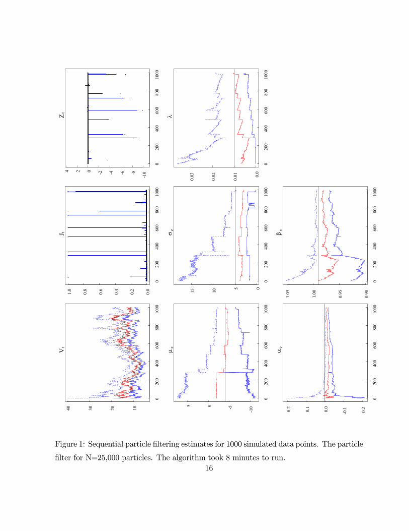
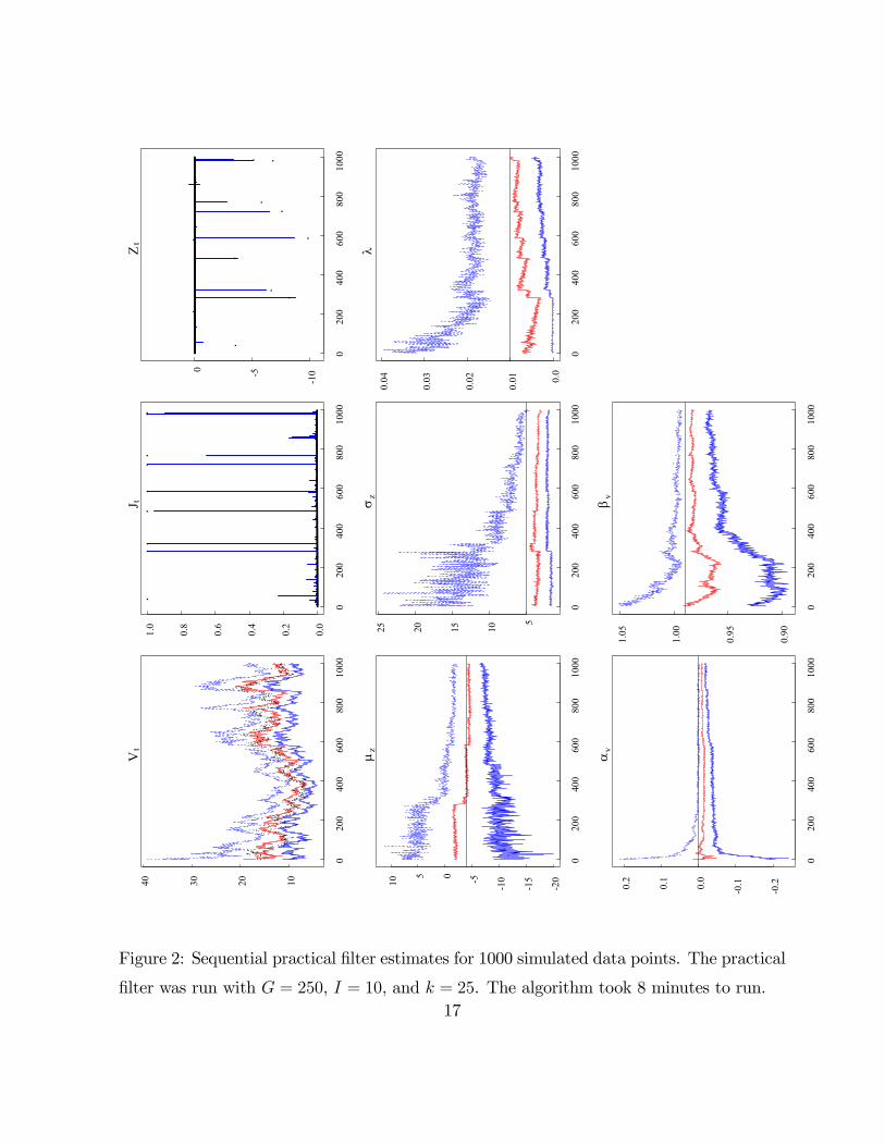
Figures 1 and 2 display the sequential posterior summaries for the particle and practical

filter, respectively. The same data were used for both filtering approaches. The top of each

subplot indicates the state variable or parameter. For the volatility (annualized) and the

parameters, the plots contain the posterior median and the (2.5,97.5)% posterior quantiles,

while the plots for the jump times and sizes contain the true jump times or sizes (dots) and

the posterior mean. In the case of jump times, the plot provides the posterior probability

that a jump occurred.

A number of points emerge. First, both algorithms are able to successfully identify

nearly all of the jumps. The only jump that was substantively missed was at data point

40 and was about -3.75%. Both algorithms identified a small jump, less than 1%, with

20% probability. As daily volatility was more than 1%, it is not difficult for the model

to generate this move with negative shock to εt and a small jump. Effectively, the jump

was too small for the algorithm to detect it. Moreover, the parameter posteriors for the

jump process the algorithm were not very informative at this early stage in the algorithm

and thus it was not able to identify the move as a jump. Both algorithms obtained similar

estimates for the other jump times and sizes.

Second, the jump parameter posteriors appear to be collapsing nicely to their true val-

ues, for both algorithms. While we begin with relatively uninformative priors, for example,

for the jump mean the (2.5,97.5)% confidence band is roughly (7,-11)%, it is evidence from

the rapid revisions in jump parameter posteriors that the sequentially estimated posterior

updates to the true parameter values. For example, at approximately data point 250 a

large jump, about -8%, arrived that was correctly identified by the algorithm. At the same

time, the posterior means for the jump mean, the jump variance, and the jump intensity

all decreased with the posterior variances falling also. Even though jumps are rare as the

15

0200

400

600

800

1000

10203040Vt

· ·· · ·· · ·· ·· ····· · ·· ·· ·· ·· ······ · · · ·· ·· ·· ·· ·· · ········ ·· · · · · ·· ·· · · ··· · ······ · · ·· · ···· ·· · · ··· · ··· ··· ···· · ·· ·· · · · · · ······ ··· · ··· ··· ······· · · ··· ·········· · · · · ·· · · · · ·· ·· ······ ····· ··

· ·· · · · · ·· ···· · · ···· ·· ···· ·· · · ······ ·· · · · ·· · ···· ··· · · · · · · ··· · ······ · · ·· ······ ·· · · · · · · ·· ···· ·· ·· ········ ·· ·· · ··· · · ··· · ·· · · ·· ·· · ·· · · ·· ·· · · · · ·· ·· · ······ ·· · · · ··· · ····· · · · · ····· · · ·· · · · ·· · · ······ ··· ·· · · ··· ·· ···· ·· ·· ·· · ··· ·· ·· ······ · · ···· · · ···· ·· · ··· ····· · · ··· · ······· · ···· · ·· ·· ·· · · ·· ·· · · ······· ··· · · ····· · · · · ·· · ·· ··· · ······ · ····· · ···· ··· · · · ········ ··· · ·· · ·· · ··· · · ·· ··· ·· · · ··· ·· ···· ··· ·· · · ·· · ··· ·· · ···· ······ ··· ··· · · ··· ····· · · · · ····· · ·· ··· · · ········ ··· ··· ···· · · · ·· ···· · · · · ··· ····· · ·· ···· · ·· · ··· · ·· ·· ···· ··· ··

· · · ·· · · · ·· ······· ···· · ·· · · · · ······· · ··· ·· ······ ··· ····· · ·· ·· ·· ·· ·· · ······ · ··· · · ·· ·· · ·· ·· ·· ····· ··· · · · · ··· ···· ·· · ·· · · ···· ······· ··· ··· ·· ····· · · ·· ·· · · ·· ····· ··· · · ··········· ··· · · ··· ·· · ·· ·· · ··· ·· · ··· ·· ·· · ·· ··· · ·· ·· ·· · ···· · · ·· ··· · ·· ··· ··· ·· · · · ···

··· · ··· · ··· · · ··· · · ·· ········ · · · · · ····· · ···· ····· · · · · ·· ······· ·· ·· ·· ··· ··

0200

400

600

800

1000

0.0

0.2

0.4

0.6

0.8

1.0

J t

··································· ········································································································································································································· ································ ········································································································································ ····················································································· ················································································································· ······································· ······································

········································································································································· ···· ···········

0200

400

600

800

1000

-10-8-6-4-2024

Zt

·································· ········································································································································································································· ······························· ········································································································································ ···················································································· ················································································································· ········································ ·······································

········································································································································ ···· ·············

0200

400

600

800

1000

-10-505

�z

0200

400

600

800

1000

05

1015

�z

0200

400

600

800

1000

0.0

0.01

0.02

0.03

�

0200

400

600

800

1000

-0.2

-0.10.0

0.1

0.2

�v

0200

400

600

800

1000

0.90

0.95

1.00

1.05

�v

Figure 1: Sequential particle filtering estimates for 1000 simulated data points. The particle

filter for N=25,000 particles. The algorithm took 8 minutes to run.16

0200

400

600

800

1000

10203040Vt

· ·· · ·· · ·· ·· ····· · ·· ·· ·· ·· ······ · · · ·· ·· ·· ·· ·· · ········ ·· · · · · ·· ·· · · ··· · ······ · · ·· · ···· ·· · ····· · ··· ··· ···· · ·· ·· ·· · · · ······ ··· · · ·· ··· ······· · · ··· ·········· · · · · ·· · · · · ·· ·· ······ ····· ··

· ·· · · · · ·· ···· · · ···· ·· ···· ·· · · ······ ·· · · · ·· · ···· ··· · · · · · · ··· · ······ · · ·· ······ ·· · · · · · · ·· ···· ·· ·· ········ ·· ·· · ··· · · ··· · ·· · ·· ·· · ·· · · ·· ·· · · · · ·· ·· · ······ ·· · · · · ·· · ···· ·· · · · ····· · · ·· · · · ··· · ······ ··· ·· · · ··· ·· ···· ·· ·· ·· · ··· ·· ·· ······ · · ···· · · ···· ·· · ··· ····· · · ··· · · ······ · ···· · ·· ·· ·· · · · ·· · · ······· ··· · · ····· · · · · ·· · ·· ··· · ······ · ····· · ···· ··· · · · ········ ··· · ·· · ·· · ··· · · ·· ··· ·· · · ··· ·· ···· ····· · · ·· · ··· ·· · ···· ······ ··· ··· · · ··· ····· · · · · ······ · ·· ··· · · ·· ········· ··· ···· · · · ·· ···· · · · · ··· ····· · ·· ···· · ·· · ··· · ·· ·· ···· ··· ··

· · · ·· · · · ·· ······· ···· · ·· · · · · ······· · ··· ·· ····· · ··· ····· · ·· ·· ·· ···· · ······ · ··· · · ·· ·· · ·· ·· ·· · ···· ··· · · · · ··· ···· ·· · ·· · · ···· ······· ··· ··· ·· ····· · · ·· ·· · · ·· ····· ··· · · ··········· ··· · · ··· ·· · ·· ·· · ··· ·· · ··· ·· ·· · ·· ··· · ·· ·· ·· · ···· · · ·· ··· · ·· ··· ····· · · · ···

··· · ··· · ··· · · ··· · · ·· ········ · · · · · ····· · ···· ····· · · · · ·· ······· ·· ·· ·· ·· · ··

0200

400

600

800

1000

0.0

0.2

0.4

0.6

0.8

1.0

J t

··································· ········································································································································································································· ································ ········································································································································ ····················································································· ················································································································· ······································· ······································

········································································································································· ···· ···········

0200

400

600

800

1000

-10-50

Zt

·································· ········································································································································································································· ······························· ········································································································································ ···················································································· ················································································································· ········································ ·······································

········································································································································ ···· ·············

0200

400

600

800

1000

-20

-15

-10-505

10

�z

0200

400

600

800

1000

5

10152025�z

0200

400

600

800

1000

0.0

0.01

0.02

0.03

0.04

�

0200

400

600

800

1000

-0.2

-0.10.0

0.1

0.2

�v

0200

400

600

800

1000

0.90

0.95

1.00

1.05

�v

Figure 2: Sequential practical filter estimates for 1000 simulated data points. The practical

filter was run with G = 250, I = 10, and k = 25. The algorithm took 8 minutes to run.17

jump intensity is one percent, the sequential estimates are able to accurately estimate the

parameters even with the small samples.

Third, the volatility parameter estimates are similar to those in Stroud, Polson and

Muller (2003). The speed of mean reversion is accurately estimated and the estimates of

αv are slightly downward biased, as is common in the literature. Fourth, as indicated in the

Figures, both algorithms are extremely computationally efficient as each algorithm takes

about 8 minutes. In the case of the practical filter, we chose the combinations of G = 250,

I = 10, and k = 25 so that the computing time was roughly equal in computing time to

the particle filter. The computational efficiency of the algorithms implies that in practice,

one could likely drastically increase N , G, I and k to obtain more accurate approximations

to the posterior while still retaining computationally feasibly algorithms.

Finally, a general comparison of the two algorithms indicates that the particle filter

posteriors are much smoother than those of the practical filter. Stroud, Polson and Muller

(2003) found that the practical filter posteriors were more accurate when compared to the

true posterior (as estimated by full sample MCMC) than those of the particle filter. It is

very likely that the practical filter is more efficiently exploring the posterior distribution

than the particle filter. A more detailed simulation design is required for more concrete

conclusions regarding the relative merits of these algorithms on simulated data.

4.2 S&P 500

To analyze the performance of the algorithms using real data, we consider daily S&P 500

index returns from January 1984 to January 2000. As in the previous case, we set σv = 0.10

and learned the other parameters. The S&P data set offers an additional challenge as it

is roughly four times as large as the simulated data. If there are degeneracies in the

algorithms, we are likely to see them more clearly in the longer time series.

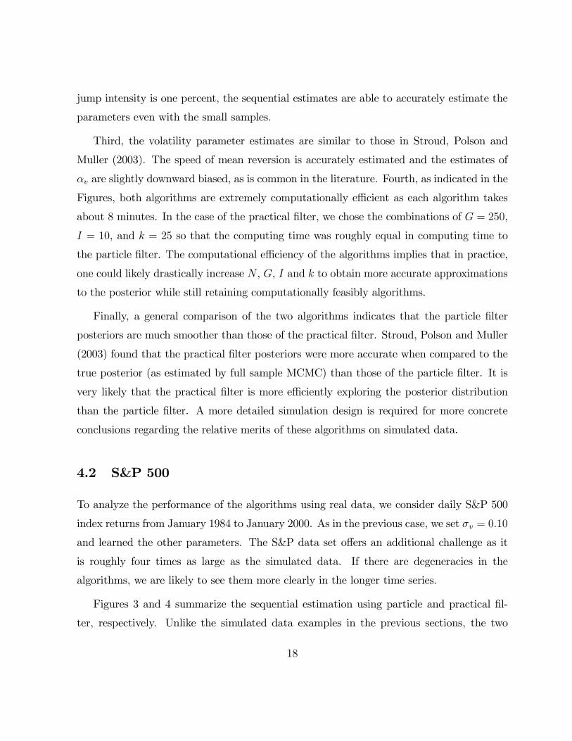
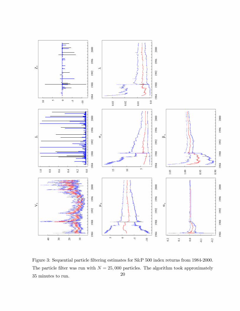
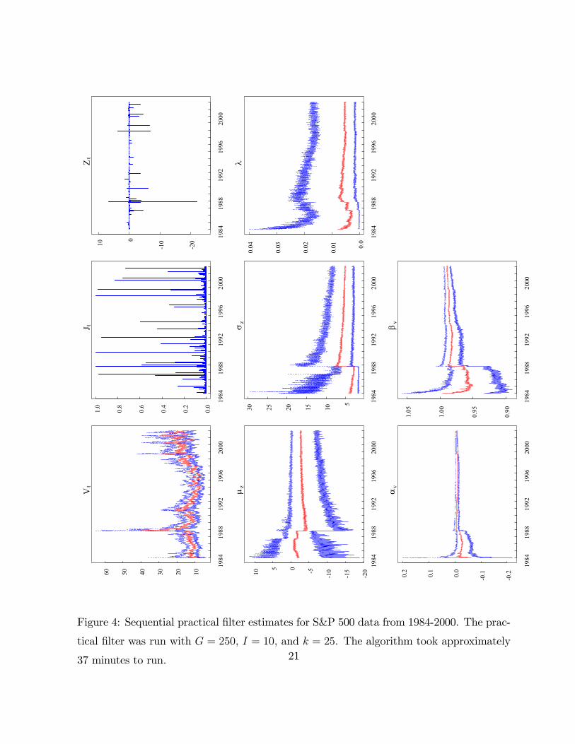
Figures 3 and 4 summarize the sequential estimation using particle and practical fil-

ter, respectively. Unlike the simulated data examples in the previous sections, the two

18

algorithms now generate some fundamental differences. First, with regard to the Crash of

1987, the two algorithms generate different state variable estimates. On October 19 and

20, 1987, the particle filter estimates jump sizes of -12% and 9% while the practical filter

estimates them to be -22% and +8% (the actual moves were -22 and 9%). In addition,

the 97.5th quantile for the volatility state peaked at about 50% for the particle filter but

was over 60% for the practical filter. Since daily volatility was less than 2% and the jump

contribution was only -12% using the particle filter, this implies that the model required

more than a 5 standard deviation shock in εt to generate the Crash. While possible, it is

highly unlikely and we conjecture that the particle filter was not able to simulate enough

particles that generated large negative jump sizes. As pointed out by Pitt and Shephard

(1999) particle filtering algorithms can have difficulties dealing with outliers.

Second, the marginal parameter posteriors for µz, σz and λ are substantively different.

For example, the posterior mean for µz with the practical filter is more negative and has

fewer spikes than the corresponding one from the particle filter. Similarly, the posterior

median for σz is higher for the practical filter. Most noticeable, the posterior confidence

bands for λ are much wider with the practical filter. This is similar to some of the findings

in Stroud, Polson and Muller (2003) who attribute it to a more accurate representation by

the practical filter. Finally, the results for αv and βv are similar for the two approaches. In

conclusion, a comparison of the two algorithms indicates they have important differences,

and we conjecture that for the given parameters and simulation scheme (choice of G, N ,

etc.), the practical filter more thoroughly samples from the posterior distribution.

5 Conclusions

This paper extends existing sequential algorithms to the case of stochastic volatility jump-

diffusion models. We find that both practical and particle filtering provide accurate infer-

ence for simulated data, while the two approaches generate substantive differences for the

S&P 500 data.

19

1984

1988

1992

1996

2000

10203040

Vt

1984

1988

1992

1996

2000

0.0

0.2

0.4

0.6

0.8

1.0

J t

1984

1988

1992

1996

2000

-10-505

10

Zt

1984

1988

1992

1996

2000

-10-505

�z

1984

1988

1992

1996

2000

5

1015

�z

1984

1988

1992

1996

2000

0.0

0.01

0.02

0.03

�

1984

1988

1992

1996

2000

-0.2

-0.10.0

0.1

0.2

�v

1984

1988

1992

1996

2000

0.90

0.95

1.00

1.05

�v

Figure 3: Sequential particle filtering estimates for S&P 500 index returns from 1984-2000.

The particle filter was run with N = 25, 000 particles. The algorithm took approximately

35 minutes to run. 20

1984

1988

1992

1996

2000

102030405060

Vt

1984

1988

1992

1996

2000

0.0

0.2

0.4

0.6

0.8

1.0

J t

1984

1988

1992

1996

2000

-20

-100

10

Zt

1984

1988

1992

1996

2000

-20

-15

-10-505

10

�z

1984

1988

1992

1996

2000

5

1015202530�z

1984

1988

1992

1996

2000

0.0

0.01

0.02

0.03

0.04

�

1984

1988

1992

1996

2000

-0.2

-0.10.0

0.1

0.2

�v

1984

1988

1992

1996

2000

0.90

0.95

1.00

1.05

�v

Figure 4: Sequential practical filter estimates for S&P 500 data from 1984-2000. The prac-

tical filter was run with G = 250, I = 10, and k = 25. The algorithm took approximately

37 minutes to run. 21

In the future, we plan a number of extensions. First, we plan more detailed simulation

experiments to further identify differences in the algorithms. For example, do either of the

algorithms rapidly degenerate as the size of the data set increases? How do the algorithms

perform with other choices for the parameters? Given the computational efficiency of the

algorithms, these simulations experiments are clearly feasible. Second, there are a number

of potential extensions which are straightforward to perform. Like Johannes, Polson and

Stroud (2002), we could consider continuous-time models and augment the state vector by

filling in missing data. Also, it would be useful to consider more general models such those

with square-root stochastic volatility and/or jumps in volatility.

Finally, as in Polson, Stroud, and Muller (2003), we found it difficult to learn the

volatility of volatility parameter, σv. There are at least two potential causes of this problem.

The marginal posterior for σv appears to have some long-memory properties, that is, data

points far in the past have a strong influence on σv. This implies that the mixing assumption

in the practical filter that observations past k-lags have little influence on the sufficient

statistics may not be appropriate. Another potential cause could lie in the high posterior

correlation between σv and βv. One potential cause of this is the prior on βv which is

normally distributed and places positive probability that βv ≥ 1. It would be interesting toinvestigate the links between stationarity assumptions on βv and estimating σv by imposing,

for example, a normal prior truncated above at βv = 1. Alternatively, there may different

parameterizations or simulation steps that can be implemented to improve the algorithms’

performance with respect to σv.

22

References

Andersen, Torben, Luca Benzoni, and Jesper Lund, 2001, Towards an empirical foundation

for continuous-time equity return models, Journal of Finance 57, 1239 - 1284.

Bakshi, Gurdip, Charles Cao, and Zhiwu Chen, 1997, Empirical performance of alternative

option pricing models, Journal of Finance 52, 2003-2049.

Bates, David, 2000, Post-’87 Crash fears in S&P 500 futures options, Journal of Econo-

metrics 94, 181-238.

Carpenter, J., , Peter Clifford., and Paul Fearnhead, 1999, An Improved Particle Filter for

Nonlinear Problems. IEE Proceedings — Radar, Sonar and Navigation, 146, 2—7.

Chernov, Mikhail, Eric Ghysels, A. Ronald Gallant, and George Tauchen, (2003), Alterna-

tive models for stock price dynamics. Forthcoming, Journal of Econometrics.

Chib, Siddhartha, Federico Nardari and Neil Shephard, 2002, Markov Chain Monte Carlo

methods for stochastic volatility models. Journal of Econometrics, 108, 281-316.

Doucet, Arnoud, Nando de Freitas, and Neil Gordon, 2001, Sequential Monte Carlo Methods

in Practice, New York: Springer-Verlag, Series Statistics for Engineering and Information

Science.

Eraker, Bjorn, Michael Johannes and Nicholas Polson, 2003, The impact of jumps in volatil-

ity and returns.” Journal of Finance 58, 1269-1300.

Gordon, Neil, D. Salmond and Adrian Smith, 1993, Novel approach to nonlinear/non-

Gaussian Bayesian state estimation. IEE Proceedings, F-140, 107—113.

Jacquier, Eric, Nicholas Polson, and Peter Rossi, 1994, Bayesian analysis of Stochastic

Volatility Models, (with discussion). Journal of Business and Economic Statistics 12, 371-

417.

Jacquier, Eric, Nicholas Polson, and Peter Rossi, 2001, Models and Priors for Multivariate

Stochastic Volatility, forthcoming, Journal of Econometrics.

23

Johannes, Michael, Nicholas Polson and Jonathan Stroud, 2001, Sequential Optimal Port-

folio Performance: Market and Volatility Timing. Working paper, Columbia University.

Johannes, Michael, Nicholas Polson and Jonathan Stroud, 2002, Nonlinear Filtering of

Stochastic Differential Equations with Jumps. Working paper, Columbia University.

Kim, Sangjoon, Neil Shephard, and Siddhartha Chib, (1998). Stochastic Volatility: Like-

lihood Inference and Comparison with ARCH Models, Review of Economic Studies 65,

361-93.

Pan, Jun, 2002, The jump-risk premia implicit in options: evidence from an integrated

time-series study, Journal of Financial Economics 63, 3—50.

Pitt, Michael and Neil Shephard, 1999, Filtering via simulation: Auxiliary particle filter,

Journal of the American Statistical Association, 590—599.

Smith, Adrian, and Alan Gelfand. (1992). Bayesian statistics without tears: a sampling-

resampling perspective, American Statistician 46, 84-88.

Storvik, Geir, 2002, Particle filters in state space models with the presence of unknown

static parameters, IEEE Trans. on Signal Processing, 50, 281—289.

Stroud, Jonathan, Nicholas Polson and Peter Müller, (2003), Practical Filtering for Sto-

chastic Volatility Models, working paper.

24