stochastic volatility in general equilibrium

Stochastic Volatility in General Equilibrium¤

George Tauchen

Department of EconomicsDuke UniversityBox 90097, Durham NC 27708, [email protected]

The connections between stock market volatility and returns are studied within thecontext of a general equilibrium framework. The framework rules out a priori anypurely statistical relationship between volatility and returns by imposing uncorre-lated innovations. The main model generates a two-factor structure for stockmarket volatility along with time-varying risk premiums on consumption andvolatility risk. It also generates endogenously a dynamic leverage effect (volatilityasymmetry), the sign of which depends upon the magnitudes of the risk aversionand the intertemporal elasticity of substitution parameters.

Keywords: Stochastic volatility; risk aversion; leverage effect; volatility asymmetry.

JEL Classification: G12, C51, C52

1. Introduction

Observers of financial markets have long noted that the volatility of financial

price movements varies stochastically. The well-established ARCH and

GARCH models of Engle (1982) and Bollerslev (1986) and the plethora of

descendants provide a very convenient framework for empirical modeling of

volatility dynamics. A somewhat different, but essentially equivalent way to

model the same phenomenon is to think in terms of the latent stochastic

*Prepared for presentation at the \Conference on Financial Econometrics" in honor of RobEngle’s Nobel Prize and presented at several meetings and conferences. The paper reflects aneffort to understand better the underlying economics of stochastic volatility, risk, return,time varying risk premiums, and the volatility risk premium. I have benefitted from many,helpful discussions with Ravi Bansal, and I am also grateful to Ivan Shaliastovich andKenneth Singleton for helpful comments. Earlier versions of the manuscript circulated on theweb, and extensions are part of (Bollerslev et al., 2009) and (Bollerslev et al., 2012).

Quarterly Journal of FinanceVol. 1, No. 4 (2011) 707�731°c World Scientific Publishing Company and Midwest Finance AssociationDOI: 10.1142/S2010139211000237

707

Qua

rt. J

. of

Fin.

201

1.01

:707

-731

. Dow

nloa

ded

from

ww

w.w

orld

scie

ntif

ic.c

omby

TSI

NG

HU

A U

NIV

ER

SIT

Y C

HIN

A o

n 10

/02/

18. R

e-us

e an

d di

stri

butio

n is

str

ictly

not

per

mitt

ed, e

xcep

t for

Ope

n A

cces

s ar

ticle

s.

http://dx.doi.org/10.1142/S2010139211000237

volatility model introduced in embryonic form by Clark (1973), extended

and formalized in Taylor (1982, 1986), and studied extensively in the vast

literature that follows (see Ghysels et al., 1996; Shephard, 2005). Financial

market empiricists now know that time varying stochastic volatility can

account for much of the dynamics of short-term financial price movements.

The empirical volatility literature has proceeded largely in a reduced form

statistical manner, with only minimal guidance from economic theory. The

role of theory has mainly been to identify important markets and sometimes

to provide informal intuitive interpretation of empirical regularities.

This paper studies stock market volatility within a self-contained general

equilibrium framework. The economy is a familiar endowment economy with

a preference structure assumed to be that of Epstein and Zin (1989) andWeil

(1989). The paper is an extension of Bansal et al. (2005), Bansal and Yaron

(2004), Campbell and Hentschell (1992), and Campbell (2003). As in those

papers, the log-linearization methods of Campbell and Shiller (1988) are

used to derive qualitative predictions and gain further insights into the

implications of the models under consideration. In this paper, however, the

volatility dynamics are more complicated. The paper proceeds through a

sequence of models, with each extension motivated by a desire to explore

more fully the relationship between stock market returns and volatility. The

models, and in particular the most general model considered in Sections 3�4

below, yield some interesting insights that can account for known charac-

teristics of stock market volatility.

For instance, empirical researchers have long known that stock market

returns and stock market volatility are negatively correlated. Black (1976) is

perhaps the first to call attention to this empirical regularity and attributes

it to changing financial leverage associated with equity prices changes, as

further studied by Christie (1982). The asymmetric effect has thus been

termed the leverage effect, and Nelson (1991) highlights its importance by

formally building the asymmetry into the E-GARCH model. Although the

term leverage effect, or simply leverage, is the common expression in the

econometrics and stochastic volatility literatures, few, if any, economists are

comfortable with the original explanation and believe the leverage effect has

more to do with risk premiums than balance sheet leverage.

Economic explanations for the leverage effect such as French et al. (1987)

employ intuitive traditional CAPM-type reasoning with a presumption that

volatility carries a positive risk premium. A related approach Campbell and

Hentschell (1992) uses the Merton (1973) model to connect expected returns

to volatility along with a GARCH-type model for the evolution of volatility.

708 � G. Tauchen

Qua

rt. J

. of

Fin.

201

1.01

:707

-731

. Dow

nloa

ded

from

ww

w.w

orld

scie

ntif

ic.c

omby

TSI

NG

HU

A U

NIV

ER

SIT

Y C

HIN

A o

n 10

/02/

18. R

e-us

e an

d di

stri

butio

n is

str

ictly

not

per

mitt

ed, e

xcep

t for

Ope

n A

cces

s ar

ticle

s.

Bekaert and Wu (2000) provide a comprehensive review of these expla-

nations and a very convenient reduced-form setup for empirical analysis of

volatility asymmetry relationships. Wu (2001) develops a self-contained

equilibrium model, along with carefully executed empirical work, but the

model relies on a pre-specified pricing kernel not directly connected to

marginal utility. Also Wu’s model permits correlations between cash flow

innovations and their volatilities that provide a statistical channel for a

leverage effect separate from any economic channels.

The main model developed and analyzed in Sections 3�4 indicates that

the existence and sign of the leverage effect depend critically on the values of

two key economic parameters, the coefficient of risk aversion and the

intertemporal elasticity of substitution. In the case of expected utility, these

parameters are reciprocals of each other, and the model predicts no leverage

effect at all in this case. Thus, the now well-established empirical finding of a

negative leverage effect �� which is reconfirmed in Figures 1 and 2 below ��strongly discredits the expected utility paradigm. Furthermore, economists

generally agree that the coefficient of risk aversion exceeds unity; if so, the

predicted sign of the leverage effect depends critically on the location of the

intertemporal elasticity of substitution relative to unity. If this elasticity

parameter exceeds unity, then the leverage effect is negative �� exactly as

observed in the data. On the other hand, if it is below unity, then the sign of

−50 −40 −30 −20 −10 0 10 20 30 40 50

−0.1

−0.05

0

0.05

0.1

0.15Dynamic Leverage Plot, VIX with S&P100 Return, Daily

Day

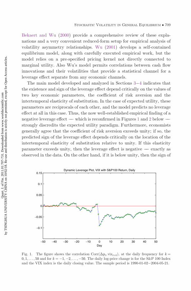
Fig. 1. The figure shows the correlation Corrð�pt ; vixtþkÞ, at the daily frequency for k ¼0; 1; . . . ; 50 and for k ¼ �1;�2; . . . ;�50. The daily log-price change is for the S&P 100 Indexand the VIX index is the daily closing value. The sample period is 1990-01-02�2004-05-21.

Stochastic Volatility in General Equilibrium � 709

Qua

rt. J

. of

Fin.

201

1.01

:707

-731

. Dow

nloa

ded

from

ww

w.w

orld

scie

ntif

ic.c

omby

TSI

NG

HU

A U

NIV

ER

SIT

Y C

HIN

A o

n 10

/02/

18. R

e-us

e an

d di

stri

butio

n is

str

ictly

not

per

mitt

ed, e

xcep

t for

Ope

n A

cces

s ar

ticle

s.

the leverage effect is positive, in direct contrast to empirical findings. The

issue of whether the intertemporal elasticity of substitution is below or above

unity is contentious; Bansal and Yaron (2005) give details on the debate.

Since the negative relationship has been so well documented, e.g., Bekaert

and Wu (2000), the findings from reduced-form modeling of asymmetric

volatility thereby have sharp consequences for an economic debate regarding

the magnitude of a key utility parameter. In addition, the model can also

explain the dynamic leverage effect, i.e., the pattern of serial cross-corre-

lations between stock market movements and volatility at different leads

and lags as documented empirically in Bollerslev et al. (2006).

The model can also account for the empirical finding that stock market

volatility appears to follow a two factor structure, with one slowly evolving

component and one quickly mean reverting component. Engle and Lee

(1999), Gallant et al. (1999), and Alizadeh et al. (2002), among many others,

adduce evidence on this empirical regularity. The two factor structure

emerges naturally from the internal structure of the model.

Finally, the model appears useful for sorting out issues related to time

varying risk prices and a volatility risk premium. A common presumption is

that, increased stock market volatility is associated with increased expected

stock market returns. This reasoning is intuitively plausible �� riskier

investments should demand a higher expected return relative to cash �� and

−6 −4 −2 0 2 4 6

−0.25

−0.2

−0.15

−0.1

−0.05

0

0.05

0.1

0.15

0.2

0.25

Dynamic Leverage Plot, VIX with S&P100 Return, Monthly

Month

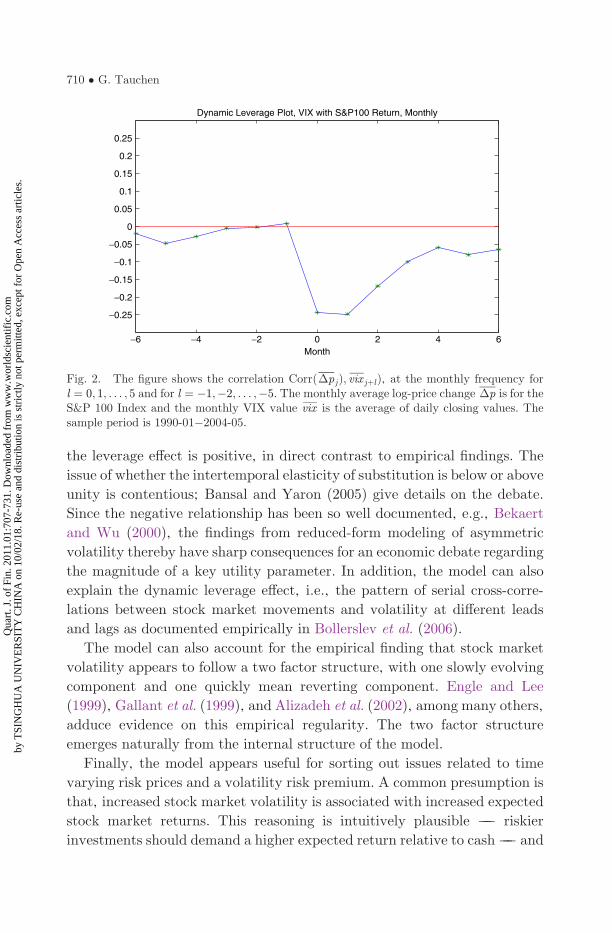
Fig. 2. The figure shows the correlation Corrð�pjÞ; vix jþlÞ, at the monthly frequency forl ¼ 0; 1; . . . ; 5 and for l ¼ �1;�2; . . . ;�5. The monthly average log-price change �p is for theS&P 100 Index and the monthly VIX value vix is the average of daily closing values. Thesample period is 1990-01�2004-05.

710 � G. Tauchen

Qua

rt. J

. of

Fin.

201

1.01

:707

-731

. Dow

nloa

ded

from

ww

w.w

orld

scie

ntif

ic.c

omby

TSI

NG

HU

A U

NIV

ER

SIT

Y C

HIN

A o

n 10

/02/

18. R

e-us

e an

d di

stri

butio

n is

str

ictly

not

per

mitt

ed, e

xcep

t for

Ope

n A

cces

s ar

ticle

s.

a rigorous analysis is Merton (1973). Various expositions of the Merton

model appear in the literature, and a convenient summary with easy to

interpret log-linear approximations is in (Campbell et al., 1997, 291�334).

An early effort to model and detect empirically the return-volatility

relationship is Bollerslev et al. (1988), who proposed the GARCH-M model

for bond returns. The follow-up literature from Nelson (1991) onwards is

huge, but, as is well known, the effort to detect an empirical relationship

between expected stock returns and volatility has yielded weak and mixed

results. Efforts such as Ghysels et al. (2005) and Lundblad (2007) employ

more powerful techniques to present evidence for a statistically significant

positive risk-return relationship, which has been here-to-for quite difficult to

detect. However, as will be seen in Section 4, such efforts are detecting the

confounding of time-varying risk premiums on consumption and volatility

risk, which clouds the interpretation of the empirical evidence. Scruggs

(1998), Guo and Whitelaw (2006), among many other studies in financial

econometrics, present evidence that additional factors are needed in the

return-volatility equation in order to measure volatility risk reliably, and the

main model below suggests the underlying variable for which these factors

are likely proxies.

The rest of this paper is organized as follows: Section 2 presents the

notation and two initial models that are useful for understanding the basic

structure and ideas. Section 3 sets forth the main model, and Section 4

connects the predictions from that model to the empirical stochastic vola-

tility literature. Section 5 contains the concluding remarks.

2. Setup, Notation, and Two Initial Models

2.1. The MRS and asset pricing

Let Mtþ1 denote the marginal rate of substitution process (MRS), also

sometimes termed the stochastic discount factor (SDF), between t and t þ 1,

and let Rtþ1 denote the gross return on an asset. The fundamental asset

pricing relationship is

EtðMtþ1Rtþ1Þ ¼ 1: ð1ÞThroughout, we shall work under a conditional lognormality assumption.

Let mtþ1 ¼ logðMtþ1Þ, and let rtþ1 ¼ logðRtþ1Þ denote the geometric return

on the asset. The fundamental asset pricing relationship is then

log½Etðemtþ1þrtþ1Þ� ¼ 0: ð2Þ


Qua

rt. J

. of

Fin.

201

1.01

:707

-731

. Dow

nloa

ded

from

ww

w.w

orld

scie

ntif

ic.c

omby

TSI

NG

HU

A U

NIV

ER

SIT

Y C

HIN

A o

n 10

/02/

18. R

e-us

e an

d di

stri

butio

n is

str

ictly

not

per

mitt

ed, e

xcep

t for

Ope

n A

cces

s ar

ticle

s.

We start by working through in this section two models that illustrate the

main points about time varying a risk premium on consumption versus a

volatility risk premium.We then proceed to themainmodel in Section 3 below.

2.2. CRR preferences and stochastic volatility

Under constant relative risk aversion (CRR) preferences Mtþ1 ¼ �ðCtþ1=

CtÞ��, where Ct is real consumption and � and � are parameters.

Equivalently,

mtþ1 ¼ � � �gtþ1; ð3Þwhere � ¼ log� and

gtþ1 ¼ ctþ1 � ct; ct ¼ logðCtÞ;so gtþ1 is the geometric growth rate of consumption. Assume the dynamics of

gtþ1 are

gtþ1 ¼ �g þ �ctzc;tþ1;

�2c;tþ1 ¼ a�c þ ��c�

2ct þ ��c�ctz�;tþ1;

ð4Þ

where �ct represents stochastic volatility in consumption that is observed by

agents but not by the econometrician, and zc;tþ1 and z�;tþ1 are iid Nð0; 1Þrandom variables. The above volatility dynamics are not quite the same as

those of Bansal and Yaron (2004) and Bansal et al. (2005), who have a con-

stant multiplying z�;tþ1, as do Brenner et al. (2006) in their continuous time

version of a setup like (4). These other papers useGaussian volatility dynamics

while (4) is a square-root, or CIR, type specification. There are certain con-

sequences to the alternative specifications as discussed further below. In

simulations, of course, care is needed to include an additional reflecting barrier

at a small positive number to ensure positivity of simulated �2c;tþ1. The above

dynamics for volatility are similar to those of Bollerslev and Zhou (2006) for

their continuous time assessment of the relationship between the expected

stock return volatility relationship.

Let vt ¼ logðPt=CtÞ denote log of the price-dividend ratio of the asset that

pays the consumption endowment fCtþjg1j¼1. Let

rtþ1 ¼ logPtþ1 þ Ctþ1

Pt

� �ð5Þ

denote the geometric return (hereafter just called the return). The standard

approximation of Campbell and Shiller (1988) log-linearization is

rtþ1 ¼ k0 þ k1vtþ1 � vt þ gtþ1; ð6Þ

712 � G. Tauchen

Qua

rt. J

. of

Fin.

201

1.01

:707

-731

. Dow

nloa

ded

from

ww

w.w

orld

scie

ntif

ic.c

omby

TSI

NG

HU

A U

NIV

ER

SIT

Y C

HIN

A o

n 10

/02/

18. R

e-us

e an

d di

stri

butio

n is

str

ictly

not

per

mitt

ed, e

xcep

t for

Ope

n A

cces

s ar

ticle

s.

where k1 < 1, k1 � 1, is a positive constant. The strategy to solve models of

this sort is to conjecture a solution for vt as a function of the state variables,

use the approximation immediately above, impose the fundamental asset

pricing equation, and then solve for the coefficients of the conjectured

solution.

In this case we conjecture

vt ¼ A0 þ A��2ct; ð7Þ

and the solutions for A0 and A� are given in Section A.1 of the Appendix.

From the solution, one can easily derive the familiar relationship for the

expected excess return

Etðrtþ1Þ � rft ¼ ��2ct �

1

2�2rt ; ð8Þ

where rft is the riskless rate in geometric form and 12 �

2rt ¼ 1

2 Vartðrtþ1Þ is a

geometric adjustment term, also called a Jensen’s Inequality adjustment

(Campbell et al., 1997, p. 307). The risk premium is thus ��2ct, and, ignoring

the geometric adjustment, one can write

rtþ1 � rft ¼ �þ ��2ct þ tþ1; ð9Þ

where � is an intercept and tþ1 is a heteroskedastic error term. This

expression is the elusive risk-return relationship sought after in the refer-

ences given above.

One has to be very careful on how to interpret the risk premium in (9),

however. It is actually a time-varying risk premium on consumption risk,

with a variable coefficient that is attributable to the stochastic volatility;

this interpretation is emphasized by Bansal and Yaron (2004) and indirectly

in (Campbell et al., 1997, p. 307). The fact that stochastic volatility gen-

erates time-varying risk premium on other factors (here consumption risk)

appears first to have made formal in an econometric sense by Bollerslev et al.

(1988), who use a GARCH-in-mean model to study the risk premium in

bond returns.

It proves interesting to examine why (9) does not reflect a volatility risk

premium. In this model, any return that depends only on the volatility

innovation z�;tþ1 carries no risk premium, despite the fact that the volatility

innovation z�;tþ1 has an impact on the return; one can easily show that

rtþ1 � Etðrtþ1Þ ¼ �ctzc;tþ1 þ k1A��c�ctz�;tþ1; ð10Þso the volatility innovation z�;tþ1 affects the return, and possibly sub-

stantially. Nonetheless, an arithmetic return that is a pure volatility bet


Qua

rt. J

. of

Fin.

201

1.01

:707

-731

. Dow

nloa

ded

from

ww

w.w

orld

scie

ntif

ic.c

omby

TSI

NG

HU

A U

NIV

ER

SIT

Y C

HIN

A o

n 10

/02/

18. R

e-us

e an

d di

stri

butio

n is

str

ictly

not

per

mitt

ed, e

xcep

t for

Ope

n A

cces

s ar

ticle

s.

such as

R�;tþ1 ¼ exp rft �1

2& 2t þ &tz�;tþ1

� �; ð11Þ

where &t is a constant known at time t, satisfies

EtðR�;tþ1Þ ¼ Rft; ð12Þwhere Rft ¼ erft ; i.e., R�;tþ1 carries no risk premium. Also, if Cð�2

c;tþ1Þ is acash flow realized at t þ 1 that only depends upon �2

c;tþ1, then the price

(present value) of that cash flow satisfies

Et½Mtþ1Cð�2c;tþ1Þ� ¼

E½Cð�2c;tþ1Þ�

Rft

: ð13Þ

There is no reward for bearing volatility risk because that risk is uncor-

related with the MRS process due to the assumption that zc;tþ1 and z�;tþ1 are

uncorrelated. Of course one could always generate a volatility risk premium

by simply correlating zc;tþ1 and z�;tþ1, but that seems ad hoc and economi-

cally unsatisfactory.

2.3. Epstein�Zin�Weil preferences and stochastic volatility

Bansal and Yaron (2004) and Bansal et al. (2005) noted that Epstein�Zin�Weil preferences can actually induce an endogenous volatility risk premium.

We start with a simplified version of their setups, point out some problems,

and then proceed to a more general version in the next section.

Write the log of the marginal rate of substitution as

mtþ1 ¼ bm0 þ bmggtþ1 þ bmrrtþ1; ð14Þand note that under Epstein�Zin�Weil preferences

bm0 ¼ logð�Þ;bmg ¼ �= ;bmr ¼ � 1;

ð15Þ

where

¼ 1� �

1� 1

: ð16Þ

The parameter � is the risk aversion parameter; is the coefficient of

intertemporal substitution, and � the subjective discount factor. If ¼ 1

then these preferences reduce to the CRR preferences studied above.

714 � G. Tauchen

Qua

rt. J

. of

Fin.

201

1.01

:707

-731

. Dow

nloa

ded

from

ww

w.w

orld

scie

ntif

ic.c

omby

TSI

NG

HU

A U

NIV

ER

SIT

Y C

HIN

A o

n 10

/02/

18. R

e-us

e an

d di

stri

butio

n is

str

ictly

not

per

mitt

ed, e

xcep

t for

Ope

n A

cces

s ar

ticle

s.

We retain the same dynamics (4) for consumption growth and volatility. The

primary differences between this setup and that of Bansal and Yaron (2004)

are that the above entails square-root volatility dynamics, instead of the

simpler Gaussian dynamics, but it excludes the long run risk factor in the

consumption growth equation. That factor is excluded only for simplification

to concentrate attention on the role of volatility.

The return on the consumption endowment rtþ1 that appears in the

expression for the log of the marginal rate of substitution (14) has to be

solved for endogenously. As before, first conjecture a solution for log price-

consumption ratio

vt ¼ A0 þ A��2ct: ð17Þ

Section A.2 of the Appendix contains the derivation of A0 and A� along with

the reduced form expressions for rtþ1 and mtþ1.

From these expressions one can deduce the expression for the expected

excess return

Etðrtþ1Þ � rft ¼ �ðbmr þ bmgÞ�2ct � bmrk

21A

2��

2�c�

2ct �

1

2�2rt ; ð18Þ

which in the case of Epstein�Zin�Weil preferences reduces to

Etðrtþ1Þ � rft ¼ ��2ct þ ð1� Þk 2

1A2��

2�c�

2ct �

1

2�2rt; ð19Þ

where again � 12 �

2rt is the geometric adjustment term. The expected excess

return

��2ct þ ð1� Þk 2

1A2��

2�c�

2ct ð20Þ

is composed of two terms. The first term represents the familiar time varying

risk premium on consumption risk, while the second represents the risk

premium on volatility. The volatility risk premium is generated endogen-

ously via the structure of the preferences, and, in fact, is absent in the CRR

case where ¼ 1. However, both risk premiums are multiples of the same

stochastic process, �2ct, and would thus be impossible to separately identify

empirically. In the expression (20) for the expected excess return, the

volatility risk premium gets confounded with the consumption risk pre-

mium. The confounding reflects the specification of stochastic volatility in

(4) above. By way of contrast, in the models of Bansal and Yaron (2004) and

Bansal et al. (2005) the volatility risk premium gets folded into a constant

term. Lettau, Ludvigson and Wachter (2008) also present a model where

there is an excess return related to consumption volatility like that of (20).


Qua

rt. J

. of

Fin.

201

1.01

:707

-731

. Dow

nloa

ded

from

ww

w.w

orld

scie

ntif

ic.c

omby

TSI

NG

HU

A U

NIV

ER

SIT

Y C

HIN

A o

n 10

/02/

18. R

e-us

e an

d di

stri

butio

n is

str

ictly

not

per

mitt

ed, e

xcep

t for

Ope

n A

cces

s ar

ticle

s.

Their model is a stochastic volatility model where volatility is governed by a

stochastic Markov regime switching variable. Like (4) above, there is a single

variable �� the volatility state �� that governs both the location and scale

of volatility, and the excess expected return is a confounding of the time

varying consumption risk premium and the volatility risk premium.

3. Main Model

Consider the following model where consumption growth is

gtþ1 ¼ �g þ �ctzc;tþ1; ð21Þas in (4), and the stochastic volatility specification is generalized to

�2c;tþ1 ¼ a�c þ ��c�

2ct þ q

12t z�;tþ1;

qtþ1 ¼ aq þ �qqt þ �qq12t zq;tþ1:

ð22Þ

Now we allow for stochastic volatility of the volatility process via the qtprocess. This characteristic of volatility is known to be empirically import-

ant; see Chernov et al. (2003) and the references therein.

The log of the marginal rate of substitution remains

mtþ1 ¼ bm0 þ bmggtþ1 þ bmrrtþ1; ð23Þwhere expressions for the coefficients are given in (15) for Epstein�Zin�Weil

preferences.

Let vt denote the log price dividend ratio of an asset paying the con-

sumption endowment and rtþ1 denote the return. Conjecture a linear

expression for vt

vt ¼ A0 þ A��2ct þAqqt; ð24Þ

where A0, A� and Aq are constants whose derivation is in Section A.3 of the

Appendix. This section of the Appendix also contains the reduced form

expressions for the marginal rate of substitution and the return. From these

expressions one can deduce that the conditional mean excess return is

Etðrtþ1Þ � rft ¼ �½ðbmr þ bmgÞ�2ct þ bmrk

21ðA2

� þ A2q�

2qÞqt � �

1

2�2rt; ð25Þ

where � 12 �

2rt ¼ � 1

2 Vartðrtþ1Þ is the geometric adjustment term. For

Epstein�Zin�Weil preferences, the conditional mean excess return reduces to

Etðrtþ1Þ � rft ¼ ��2ct þ ð1� Þk 2

1ðA2� þ A2

q�2qÞqt �

1

2�2rt: ð26Þ

716 � G. Tauchen

Qua

rt. J

. of

Fin.

201

1.01

:707

-731

. Dow

nloa

ded

from

ww

w.w

orld

scie

ntif

ic.c

omby

TSI

NG

HU

A U

NIV

ER

SIT

Y C

HIN

A o

n 10

/02/

18. R

e-us

e an

d di

stri

butio

n is

str

ictly

not

per

mitt

ed, e

xcep

t for

Ope

n A

cces

s ar

ticle

s.

The risk premium

��2ct þ ð1� Þk 2

1ðA2� þ A2

q�2qÞqt; ð27Þ

is composed of two separate terms, where the first term reflects the risk

premium on consumption risk and the second the risk premium on volatility

risk. The second term confounds the risk premium on shocks to volatility,

z�;tþ1, with the premium on shocks to the volatility of volatility, zq;tþ1, but

nonetheless this risk premium (or more precisely the risk price) can be sep-

arately identified from that of consumption risk. Indeed, Scruggs (1998) and

Guo andWhitelaw (2006) present evidence that additional control factors are

needed in the return-volatility equation in order to estimate reliably the

relationship between expected return and volatility. In both cases, the

additional factors include at least one interest rate variable, which is arguable

a proxy for qt in the equation immediately above, given that the level of

interest rates is associated with the turbulence of financial markets. Guo et al.

(2009) suggested that the value premium needs to be included, which is the

likely prediction of a model like this one but with a long run risk factor. In a

somewhat different vein, Adrian andRosenberg (2007) find empirical evidence

that a two-factor type structure is helpful for explaining the cross-section of

expected asset returns.

Interestingly, the sign of the volatility risk premium depends critically on

the sign of 1� , where is defined in (16). Most economists would probably

agree that � > 1, i.e., the agent is more risk averse than a log investor. If

� > 1, then the sign of

1� ¼� � 1

1� 1

ð28Þ

depends upon . A sufficient condition for a positive volatility risk premium

is > 1, which Bansal and Yaron (2004) argue is the most reasonable region

for . On the other hand, a number of economists such as Campbell and Koo

(1997) (and references therein) argue that < 1. If so, then it would take

rather small values of to generate a positive risk premium on volatility

since

1

�) 1� > 0; ð29Þ

1

�< < 1 ) 1� < 0: ð30Þ


Qua

rt. J

. of

Fin.

201

1.01

:707

-731

. Dow

nloa

ded

from

ww

w.w

orld

scie

ntif

ic.c

omby

TSI

NG

HU

A U

NIV

ER

SIT

Y C

HIN

A o

n 10

/02/

18. R

e-us

e an

d di

stri

butio

n is

str

ictly

not

per

mitt

ed, e

xcep

t for

Ope

n A

cces

s ar

ticle

s.

4. Stock Price and Volatility Dynamics

Much of the stochastic volatility literature examines the log capital return

process

�pt ¼ logðPtÞ � logðPt�1Þ ð31Þinstead of the total return process, rt, which includes the dividend yield. In

this section, we shall study the dynamics of the volatility of �pt implied by

the general stochastic volatility model of Section 3; the conclusions are

essentially the same for either process, because the capital gain return tends

to dominate the total return.

The reduced form expression for the �pt process is derived in the Sec-

tion A.3 of the Appendix and takes the form

�pt ¼ bp0 þ A�ð��c � 1Þ�2c;t�1 þ Aqð�q � 1Þqt�1

þ �c;t�1zc;t þA�q12t�1z�;t þ Aq�qq

12t�1zq;t; ð32Þ

where bp0 is a constant and the other parameters are defined in Section A.3 of

the Appendix. Note that from (A.48) A� is of the form

A� ¼1

h�; h� > 0; ð33Þ

and from (A.49) Aq is of the form

Aq ¼1

hq; hq > 0; ð34Þ

and so the signs of A� and Aq are same as those of defined in (16) above.

We consider first the dynamic relationship between �pt and the con-

sumption volatility process �2ct. It follows from the expression (32) and the

dynamics (22) that

Covð�pt ; �2�c;t�jÞ ¼ A�ð�� 1ÞEð�4

c;t�1Þ� j�1�c ; j ¼ 1; 2; . . . ;1;

Covð�pt ; �2ctÞ ¼ �qA�ð��c � 1ÞEð�4

c;t�1Þ þ A�Eðqt�1Þ;Covð�pt ; �

2c�;tþjÞ ¼ A�ð�� 1ÞEð�4

c;t�1Þ� j�c; j ¼ 1; 2; . . . ;1:

ð35Þ

The serial cross-covariances Covð�pt; �2c;tþjÞ for j 6¼ 0 are proportional to the

autocovariance function of the �2ct process. The sign will be negative if < 0,

as would be the case if both � and exceed unity. Thus, in this case a market

price decline would signal increased future expected consumption volatility,

a result analogous to that of who study the covariance between the log price

dividend ratio, vt, and subsequent consumption volatility �c;tþj, j > 0.

718 � G. Tauchen

Qua

rt. J

. of

Fin.

201

1.01

:707

-731

. Dow

nloa

ded

from

ww

w.w

orld

scie

ntif

ic.c

omby

TSI

NG

HU

A U

NIV

ER

SIT

Y C

HIN

A o

n 10

/02/

18. R

e-us

e an

d di

stri

butio

n is

str

ictly

not

per

mitt

ed, e

xcep

t for

Ope

n A

cces

s ar

ticle

s.

Interestingly, the sign of the contemporaneous covariance Covð�2ct ;�ptÞ is

ambiguous because it is the sum of terms of opposite signs.

To tie the theory to the stochastic volatility literature, the most inter-

esting series is the one-step conditional variance process defined as

�2pt � Vartð�ptþ1Þ ¼ �2

ct þ ðA2� þ A2

q�2qÞqt : ð36Þ

From (36) it is immediately seen that conditional volatility follows a

two-factor structure where it is the superposition of two autoregressive

processes. This theoretical representation of volatility corresponds exactly

to the two-factor structure found empirically in Engle and Lee (1999) and

an extensive subsequent literature. The typical structure identified

empirically contains one factor that is extremely persistent and another

that is strongly mean reverting and nearly serially uncorrelated. In (36),

�2ct is a likely candidate for the persistent factor while qt is likely the

strongly mean reverting factor. Scruggs (1998) and Guo and Whitelaw

(2006) present evidence that additional factor(s) are needed in the return-

volatility equation in order to empirically measure volatility risk reliably.

These factors are variables that tend to be high when financial volatility

is high. Their findings appear completely consistent with Eq. (36),

which suggests that these factors should be related to qt, the volatility of

volatility.

The contemporaneous leverage effect pertains to the correlation between

the conditional volatility process �2pt and the capital return process �pt . An

easily computed conditional moment is

Covt�1ð�pt; �2ptÞ ¼ A�qt�1 þ AqðA2

� þ A2q�

2Þqt�1: ð37Þ

One sees immediately from these covariances along with with (33), (34),

and (16) the role that the utility function parameters � and play in

determining the sign of the leverage effect. The covariances are negative

under the parameter values utilized by Bansal and Yaron (2004) for their

calibrations.

We now consider the dynamic leverage effect. Some direct empirical

evidence is seen in Figure 1, which shows the correlations between �p as

proxied by the logarithmic return on S&P 100 Index and leads and lags of the

VIX volatility Index, daily, 1990�2004. The VIX index is designed to reflect

the implied volatility on S&P 100 Index options with one month to

expiration. Evidently, a large price increase is associated with a con-

temporaneous drop in volatility which then slowly dies away. Figure 2 shows


Qua

rt. J

. of

Fin.

201

1.01

:707

-731

. Dow

nloa

ded

from

ww

w.w

orld

scie

ntif

ic.c

omby

TSI

NG

HU

A U

NIV

ER

SIT

Y C

HIN

A o

n 10

/02/

18. R

e-us

e an

d di

stri

butio

n is

str

ictly

not

per

mitt

ed, e

xcep

t for

Ope

n A

cces

s ar

ticle

s.

the same correlations except computed using monthly averages. The pattern

remains quite apparent at the monthly frequency. Both figures are consistent

with the evidence adduced in Bollerslev et al. (2006) using very high

frequency data.

Table 1. Parameter settings CasesA and B.

Parameter Case A Case B

a�c 0.10e-06 0.10e-06��c 0.98 0.98aq 0.20e-06 0.20e-06

�q 0.20 0.20

�q 0.10e-06 0.10e-06

� 0.9949 0.9949� 8.00 8.00 1.50 0.50�c 0.163e-02 0.163e-02

−50 −40 −30 −20 −10 0 10 20 30 40 50−0.2

0

0.2

0.4

0.6

0.8

Autocorrelations of Conditional Volatility, Case A:ψ=1.50

−50 −40 −30 −20 −10 0 10 20 30 40 50−0.2

0

0.2

0.4

0.6

0.8

Autocorrelations of Conditional Volatility, Case B:ψ=0.50

Fig. 3. Each panel shows the autocorrelation function of the conditional variance process:Corrð�2

pt ; �2p;tþjÞ, j ¼ �50; . . . ; 50. The top panel is computed under the parameter settings A

of Table 1, where the inter-temporal elasticity of substitution is ¼ 1:50; the bottom panel iscomputed under settings B of Table 1, where the inter-temporal elasticity of substitution is ¼ 0:50. Comparison of the two panels indicates that the the autocorrelation function of theconditional variance process is very insensitive to the value of .

720 � G. Tauchen

Qua

rt. J

. of

Fin.

201

1.01

:707

-731

. Dow

nloa

ded

from

ww

w.w

orld

scie

ntif

ic.c

omby

TSI

NG

HU

A U

NIV

ER

SIT

Y C

HIN

A o

n 10

/02/

18. R

e-us

e an

d di

stri

butio

n is

str

ictly

not

per

mitt

ed, e

xcep

t for

Ope

n A

cces

s ar

ticle

s.

In order to compare the predictions from the model to the observed

pattern, we need to compute analogous correlations under the model.

Convenient analytical approximate results involving moments of �2pt and

cross-moments with other series appear to be out of reach. Instead, simu-

lation is used to compute unconditional correlations of interest. Given a set

of parameter values, the model of Section 3 is simulated for 10,000 periods

and population moments implied by the model are computed via Monte

Carlo. Following the recommendation of Campbell and Koo (1997) the

orthogonality conditions of the Euler equation error were checked and found

to be negligible.

The correlations of interest are computed for two sets of parameter

values, labeled Cases A and B in Table 1, which are based on Campbell and

Koo (1997) and Bansal, Gallant and Tauchen (2004). The only difference

−50 −40 −30 −20 −10 0 10 20 30 40 50

−0.2

−0.1

0

0.1

0.2

Dynamic Leverage Correlations, Case A:ψ=1.50

−50 −40 −30 −20 −10 0 10 20 30 40 50

−0.2

−0.1

0

0.1

0.2

Dynamic Leverage Correlations, Case B:ψ=0.50

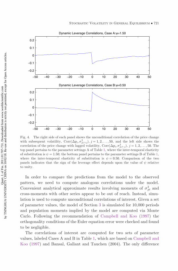
Fig. 4. The right side of each panel shows the unconditional correlation of the price changewith subsequent volatility, Corr(�pt ; �

2p;tþjÞ; j ¼ 1; 2; . . . ; 50, and the left side shows the

correlation of the price change with lagged volatility, Corrð�pt ; �2p;t�jÞ, j ¼ 1; 2; . . . ; 50. The

top panel pertains to the parameter settings A of Table 1, where the inter-temporal elasticityof substitution is ¼ 1:50; the bottom panel pertains to the parameter settings B of Table 1,where the inter-temporal elasticity of substitution is ¼ 0:50. Comparison of the twopanels indicates that the sign of the leverage effect depends upon the value of relativeto unity.


Qua

rt. J

. of

Fin.

201

1.01

:707

-731

. Dow

nloa

ded

from

ww

w.w

orld

scie

ntif

ic.c

omby

TSI

NG

HU

A U

NIV

ER

SIT

Y C

HIN

A o

n 10

/02/

18. R

e-us

e an

d di

stri

butio

n is

str

ictly

not

per

mitt

ed, e

xcep

t for

Ope

n A

cces

s ar

ticle

s.

between the two cases is that the elasticity of substitution ¼ 1:50 in A

and ¼ 0:50 in B. The risk aversion parameter � is the same in both cases.

The other values of the parameters would be reasonable for a model oper-

ating in monthly time. The model could not be expected to fit actual data

because it lacks a long run risk component in consumption growth, which is

left out only for simplicity. Figure 3 shows the autocorrelation function of

stock market volatility �2pt for the two sets parameter settings. The per-

sistence of volatility is completely consistent with all empirical findings, and

comparison across cases indicates that the value of the elasticity of substi-

tution has little effect on volatility persistence.

Figure 4 shows predicted dynamic leverage correlations between �pt and

leads and lags of �2pt. In the upper panel, where ¼ 1:50, the contemporaneous

leverage effect is a negative and it fades away over time, which is completely

consistent with Figures 1 and 2. In the bottom panel, where ¼ 0:50, the

leverage effect is positive, which is completely counter factual. Interestingly,

and somewhat surprisingly, the observed negative dynamic leverage effect

is fairly compelling evidence for an intertemporal elasticity of substitution

above unity.

5. Conclusion

The characteristics of the relationships between stock market volatility

and stock market returns are examined within the context of a general

equilibrium framework. The framework only permits connections between

volatility and returns that arise through the internal economic structure of

the model. All innovations are presumed uncorrelated, thereby ruling out

connections that could arise via separate statistical channels. The most

general model generates a two-factor structure for volatility along with

time-varying risk premiums on consumption and volatility risk. It also

generates endogenously a dynamic leverage effect, the sign of which

depends upon the magnitudes of the risk aversion (�) and intertemporal

elasticity of substitution ( ) parameters. In the case of expected utility

where � ¼ 1= , the leverage effect is absent, which suggest a strong con-

nection between non-expected utility preferences and the leverage effect.

The magnitude of relative to unity is an issue of debate in the financial

economics literature. Interestingly, if � > 1, as is commonly presumed,

then the observed negative leverage effect necessarily implies > 1, so the

well documented finding of negative leverage has bearing on this economic

debate.

722 � G. Tauchen

Qua

rt. J

. of

Fin.

201

1.01

:707

-731

. Dow

nloa

ded

from

ww

w.w

orld

scie

ntif

ic.c

omby

TSI

NG

HU

A U

NIV

ER

SIT

Y C

HIN

A o

n 10

/02/

18. R

e-us

e an

d di

stri

butio

n is

str

ictly

not

per

mitt

ed, e

xcep

t for

Ope

n A

cces

s ar

ticle

s.

Appendix. Details of the Derivations

A.1. Solution for the model with CRR preferences

in Section 2.2

From the approximation rtþ1 ¼ k0 þ k1vtþ1 � vt þ gtþ1 and the presumed

dynamics for gtþ1 and �2c;tþ1 it follows that

rtþ1 ¼ k0 þ ðk1 � 1ÞA0 þ k1A�a�c þ �c þ A�ðk1��c � 1Þ�2ct

þ k1��cA��ctz�;tþ1 þ �ctzc;tþ1 ðA:1Þand

mtþ1 ¼ � � ��c � ��ctzc;tþ1: ðA:2ÞThus,

Etðertþ1þmtþ1Þ ¼ 1 ) ðA:3Þ

Etðrtþ1 þmtþ1Þ þ1

2Vartðrtþ1 þmtþ1Þ ¼ 0: ðA:4Þ

Computing the conditional first two moments and setting the above to zero

gives

k0 þ ðk1 � 1ÞA0 þ k1A�a�c þ � þ ð1� �Þ�cþ A�ðk1��c � 1Þ þ 1

2k 21�

2�cA

2� þ

1

2ð1� �Þ2

� ��2ct ¼ 0: ðA:5Þ

This can hold for all values of �2ct only if

A0 ¼k0 þ k1A�a�c þ � þ ð1� �Þ�c

1� k1; ðA:6Þ

where A� is a solution to the quadratic

ð1� �Þ2 þ 2ðk1��c � 1ÞA� þ k 21�

2�cA

2� ¼ 0: ðA:7Þ

There are two roots

Aþ;�� ¼ 1� k1��c �

ffiffiffiffiffiffiffiffiffiffiffiffiffiffiffiffiffiffiffiffiffiffiffiffiffiffiffiffiffiffiffiffiffiffiffiffiffiffiffiffiffiffiffiffiffiffiffiffiffiffiffiffiffiffiffiffiffiffiffiffið1� k1��cÞ2 � ð1� �Þ2k 2

1�2�c

pk 21�

2�c

; ðA:8Þ

which are real so long as �2�c is sufficiently small. The root Aþ

� has the

unappealing property that

lim��c!0

Aþ� �

2�c 6¼ 0; ðA:9Þ


Qua

rt. J

. of

Fin.

201

1.01

:707

-731

. Dow

nloa

ded

from

ww

w.w

orld

scie

ntif

ic.c

omby

TSI

NG

HU

A U

NIV

ER

SIT

Y C

HIN

A o

n 10

/02/

18. R

e-us

e an

d di

stri

butio

n is

str

ictly

not

per

mitt

ed, e

xcep

t for

Ope

n A

cces

s ar

ticle

s.

which would mean the impact of �ct would grow without bound as stochastic

volatility becomes unimportant. Thus we take A�� as the economically

meaningful root and set

A� ¼1� k1��c �


1�2�c

pk 21�

2�c

: ðA:10Þ

A.2. Solution for model with EZW preferences in Section 2.3

From the approximation rtþ1 ¼ k0 þ k1vtþ1 � vt þ gtþ1 and the presumed

dynamics for gtþ1 and �2c;tþ1 it follows that

rtþ1 ¼ k0 þ ðk1 � 1ÞA0 þ k1A�a�c þ �c þA�ðk1��c � 1Þ�2ct

þ k1��cA��ctz�;tþ1 þ �ctzc;tþ1; ðA:11Þwith

mtþ1 ¼ bm0 þ bmggtþ1 þ bmrrtþ1: ðA:12ÞThen,

mtþ1 ¼ bm0 þ bmg�c

þ bmr ½k0 þ ðk1 � 1ÞA0 þ k1A�a�c þ �c þ A�ðk1��c � 1Þ�2ct�

þ bmrk1��cA��ctz�;tþ1 þ ðbmr þ bmgÞ�ctzc;tþ1: ðA:13ÞThus,

rtþ1 þmtþ1 ¼ ð1þ bmrÞ½k0 þ ðk1 � 1ÞA0 þ k1A�a�c�þ ð1þ bmr þ bmgÞ�c þ bm0 þ ð1þ bmrÞ½A�ðk1��c � 1Þ��2

ct

þ ð1þ bmrÞk1��cA��ctz�;tþ1 þ ð1þ bmr þ bmgÞ�ctzc;tþ1;

ðA:14Þand

Etðrtþ1 þmtþ1Þ ¼ ð1þ bmrÞ½k0 þ ðk1 � 1ÞA0 þ A�k1a�c�þ ð1þ bmr þ bmgÞ�c þ bm0 þ ð1þ bmrÞ½A�ðk1��c � 1Þ��2

ct ;

ðA:15ÞVartðrtþ1 þmtþ1Þ ¼ ½ð1þ bmrÞ2k 2

1�2�cA

2� þ ð1þ bmr þ bmgÞ2��2

ct : ðA:16ÞImposing

Etðrtþ1 þmtþ1Þ þ1

2Vartðrtþ1 þmtþ1Þ ¼ 0; ðA:17Þ

724 � G. Tauchen

Qua

rt. J

. of

Fin.

201

1.01

:707

-731

. Dow

nloa

ded

from

ww

w.w

orld

scie

ntif

ic.c

omby

TSI

NG

HU

A U

NIV

ER

SIT

Y C

HIN

A o

n 10

/02/

18. R

e-us

e an

d di

stri

butio

n is

str

ictly

not

per

mitt

ed, e

xcep

t for

Ope

n A

cces

s ar

ticle

s.

and equating to zero the constant and coefficient of �2ct gives the equations

0 ¼ ð1þ bmrÞ½k0 þ ðk1 � 1ÞA0 þ k1A�a�c� þ ð1þ bmr þ bmgÞ�c þ bm0;

ðA:18Þ

0 ¼ ð1þ bmrÞðk1��c � 1ÞA� þ1

2½ð1þ bmrÞ2k 2

1�2�cA

2� þ ð1þ bmr þ bmgÞ2�:

ðA:19ÞThus,

A0 ¼k0 þ k1A�a�c

ð1� k1Þþ ð1þ bmr þ bmgÞ�c þ bm0

ð1þ bmrÞð1� k1Þ; ðA:20Þ

where A� is the solution of the quadratic

ð1þ bmr þ bmgÞ2 þ 2ð1þ bmrÞðk1��c � 1ÞA� þ ð1þ bmrÞ2k 21�

2�cA

2� ¼ 0:

ðA:21ÞThere are two roots

Aþ;�� ¼

1� k1��c �ffiffiffiffiffiffiffiffiffiffiffiffiffiffiffiffiffiffiffiffiffiffiffiffiffiffiffiffiffiffiffiffiffiffiffiffiffiffiffiffiffiffiffiffiffiffiffiffiffiffiffiffiffiffiffiffiffiffiffiffiffiffiffiffiffiffiffiffiffiffiffiffiffiffiffiffið1� k1��cÞ2 � ð1þ bmr þ bmgÞ2k 2

1�2�c

qð1þ bmrÞk 2

1�2�c

: ðA:22Þ

The root Aþ� has the unappealing property that

lim� 2�c!0

�2�cA

þ� 6¼ 0; ðA:23Þ

so we take A�� as the economically meaningful root and set

A� ¼1� k1��c �

ffiffiffiffiffiffiffiffiffiffiffiffiffiffiffiffiffiffiffiffiffiffiffiffiffiffiffiffiffiffiffiffiffiffiffiffiffiffiffiffiffiffiffiffiffiffiffiffiffiffiffiffiffiffiffiffiffiffiffiffiffiffiffiffiffiffiffiffiffiffiffiffiffiffiffiffið1� k1��cÞ2 � ð1þ bmr þ bmgÞ2k 2

1�2�c

qð1þ bmrÞk 2

1�2�c

: ðA:24Þ

In the case of Epstein�Zin�Weil preferences the coefficients are

A0 ¼k0 þ k1A�a�c

ð1� k1Þþ ð1� �Þ�c þ logð�Þ

ð1� k1Þ; ðA:25Þ

A� ¼1� k1��c �


1�2�c

pk 2

1�2�c

: ðA:26Þ

It is useful to record the reduced form expression for mtþ1, rtþ1:

mtþ1 ¼ b�m0 þ bmrA�ðk1��c � 1Þ�2ct þ ðbmr þ bmgÞ�ctzc;tþ1

þ bmrk1A��c�ctz�;tþ1; ðA:27Þrtþ1 ¼ br0 þ A�ðk1��c � 1Þ�2

ct þ �ctzc;tþ1 þ k1A��c�ctz�;tþ1; ðA:28Þ


Qua

rt. J

. of

Fin.

201

1.01

:707

-731

. Dow

nloa

ded

from

ww

w.w

orld

scie

ntif

ic.c

omby

TSI

NG

HU

A U

NIV

ER

SIT

Y C

HIN

A o

n 10

/02/

18. R

e-us

e an

d di

stri

butio

n is

str

ictly

not

per

mitt

ed, e

xcep

t for

Ope

n A

cces

s ar

ticle

s.

where b�m0 and br0 are readily determined constants. In the case of

Epstein�Zin�Weil preferences the reduced form expressions are

mtþ1 ¼ b�m0 þ ð� 1ÞA�ðk1��c � 1Þ�2ct � ��ctzc;tþ1 þ ð� 1Þk1A��c�ctz�;tþ1;

rtþ1 ¼ br0 þ A�ðk1��c � 1Þ�2ct þ �ctzc;tþ1 þ k1A��c�ctz�;tþ1:

ðA:29Þ

A.3. Solution for the model with EZW preferences and general

stochastic volatility in Section 3

The steps to find the solution start with

rtþ1 ¼ k0 þ ðk1 � 1ÞA0 þ A�ðk1�2c;tþ1 � �2

ctÞþ Aqðk1qtþ1 � qtÞ þ gtþ1: ðA:30Þ

Thus,

mtþ1 þ rtþ1 ¼ bm0 þ ð1þ bmrÞ½k0 þ ðk1 � 1ÞA0� þ ð1þ bmg þ bmrÞgtþ1

þ ð1þ bmrÞ½A�ðk1�2c;tþ1 � �2

ctÞ þ Aqðk1qtþ1 � qtÞ�; ðA:31Þand so,

Etðmtþ1 þ rtþ1Þ ¼ bm0 þ ð1þ bmrÞ½k0 þ ðk1 � 1ÞA0� þ ð1þ bmg þ bmrÞ�gþ ð1þ bmrÞk1½A�a�c þ Aqaq�þ ð1þ bmrÞ½A�ðk1��c � 1Þ�2

ct þ Aqðk1�q � 1Þqt �; ðA:32Þand

Vartðmtþ1 þ rtþ1Þ ¼ Vart ½ð1þ bmg þ bmrÞgtþ1�þ Vart½ð1þ bmrÞðA�k1�

2c;tþ1 þ Aqk1qtþ1Þ�: ðA:33Þ

This can be expressed as

Vartðmtþ1 þ rtþ1Þ ¼ ð1þ bmg þ bmrÞ2�2ct

þ ð1þ bmrÞ2ðA2�k

21qt þ A2

qk21�

2qqtÞ: ðA:34Þ

The asset pricing equation is

0 ¼ Etðmtþ1 þ rtþ1Þ þ1

2Vartðmtþ1 þ rtþ1Þ: ðA:35Þ

Setting to zero, the constant term yields

A0 ¼bm0 þ ð1þ bmrÞ½k0 þ k1ðA�a�c þ AqaqÞ� þ ð1þ bmg þ bmrÞ�c

ð1þ bmrÞð1� k1Þ: ðA:36Þ

726 � G. Tauchen

Qua

rt. J

. of

Fin.

201

1.01

:707

-731

. Dow

nloa

ded

from

ww

w.w

orld

scie

ntif

ic.c

omby

TSI

NG

HU

A U

NIV

ER

SIT

Y C

HIN

A o

n 10

/02/

18. R

e-us

e an

d di

stri

butio

n is

str

ictly

not

per

mitt

ed, e

xcep

t for

Ope

n A

cces

s ar

ticle

s.

The term for �2ct is

ð1þ bmrÞðk1��c � 1ÞA��2ct þ

1

2ð1þ bmg þ bmrÞ2�2

ct; ðA:37Þ

and setting it to zero gives

A� ¼12 ð1þ bmg þ bmrÞ2

ð1þ bmrÞð1� k1��cÞ: ðA:38Þ

The term for qt is

ð1þ bmrÞðk1�q � 1ÞAqqt þ1

2ð1þ bmrÞ2ðA2

�k21qt þ A2

qk21�

2qqtÞ; ðA:39Þ

and setting it to zero gives a quadratic in Aq:

ð1þ bmrÞA2�k

21 þ 2ðk1�q � 1ÞAq þ ð1þ bmrÞk 2

1�2qA

2q ¼ 0: ðA:40Þ

There are two real solutions

Aþq ;A

�q ¼

1� k1�q �ffiffiffiffiffiffiffiffiffiffiffiffiffiffiffiffiffiffiffiffiffiffiffiffiffiffiffiffiffiffiffiffiffiffiffiffiffiffiffiffiffiffiffiffiffiffiffiffiffiffiffiffiffiffiffiffiffiffiffiffiffiffiffiffiffiffið1� k1�qÞ2 � ð1þ bmrÞ2k 4

1�2qA

2�

qð1þ bmrÞk 2

1�2q

; ðA:41Þ

so long as

�2q �

ð1� k1�qÞ2ð1þ bmrÞ2k 4

1A2�

: ðA:42Þ

Note that,

lim�q!0

�2qA

þq 6¼ 0; ðA:43Þ

which is economically unappealing, so we take the other root and set

Aq ¼1� k1�q �

ffiffiffiffiffiffiffiffiffiffiffiffiffiffiffiffiffiffiffiffiffiffiffiffiffiffiffiffiffiffiffiffiffiffiffiffiffiffiffiffiffiffiffiffiffiffiffiffiffiffiffiffiffiffiffiffiffiffiffiffiffiffiffiffiffiffið1� k1�qÞ2 � ð1þ bmrÞ2k 4

1�2qA

2�

qð1þ bmrÞk 2

1�2q

: ðA:44Þ

The solution for the log price dividend ratio is thus

vt ¼ A0 þA��2ct þ Aqqt ; ðA:45Þ

where expressions for A0, A� and Aq are given immediately above. Under

Epstein�Zin�Weil preferences the coefficients are

A0 ¼½logð�Þ þ k0 þ k1ðA�a�c þAqaqÞ� þ ð1� �Þ�c

ð1� k1ÞðA:46Þ


Qua

rt. J

. of

Fin.

201

1.01

:707

-731

. Dow

nloa

ded

from

ww

w.w

orld

scie

ntif

ic.c

omby

TSI

NG

HU

A U

NIV

ER

SIT

Y C

HIN

A o

n 10

/02/

18. R

e-us

e an

d di

stri

butio

n is

str

ictly

not

per

mitt

ed, e

xcep

t for

Ope

n A

cces

s ar

ticle

s.

or

A0 ¼logð�Þ þ k0 þ k1ðA�a�c þAqaqÞ

1� k1þ ð1� �Þ�cð1� k1Þ

; ðA:47Þ

and

A� ¼12 ð1� �Þ2ð1� k1��cÞ

; ðA:48Þ

Aq ¼1� k1�q �

ffiffiffiffiffiffiffiffiffiffiffiffiffiffiffiffiffiffiffiffiffiffiffiffiffiffiffiffiffiffiffiffiffiffiffiffiffiffiffiffiffiffiffiffiffiffiffiffiffiffið1� k1�qÞ2 � 2k 4

1�2qA

2�

qk 2

1�2q

: ðA:49Þ

The reduced form expressions for the MRS, the return, and the price

change, are derived as follows. Start with

mtþ1 ¼ bm0 þ bmggtþ1 þ bmrrtþ1; ðA:50Þmtþ1 ¼ bm0 þ bmg�c þ bmg�ctzc;tþ1 þ bmrðk0 þ k1vtþ1 � vt þ gtþ1Þ: ðA:51Þ

Hence,

mtþ1 ¼ b�m0þ bmrA�ðk1��c� 1Þ�2ct þ bmrAqðk1�q � 1Þqt

þ ðbmg þ bmrÞ�ctzc;tþ1þ bmrk1A�q12t z�;tþ1þ bmrk1Aq�qq

12t zq;tþ1; ðA:52Þ

where

b�m0 ¼ bm0 þ ðbmg þ bmrÞ�c þ bmr ½k0 þ k1ðA�a�c þAqaqÞ�þ bmrðk1 � 1ÞA0: ðA:53Þ

Under Epstein�Zin�Weil preferences the solution for the MRS is

mtþ1 ¼ b�m0 þ ð� 1ÞA�ðk1��c � 1Þ�2ct þ ð� 1ÞAqðk1�q � 1Þqt

� ��ctzc;tþ1 þ ð� 1Þk1A�q12t z�;tþ1 þ ð� 1Þk1Aq�qq


with

b�m0 ¼ logð�Þ � ��g þ ð� 1Þ½k0 þ k1ðA�a�c þ AqaqÞ�þ ð� 1Þðk1 � 1ÞA0: ðA:55Þ

To obtain the reduced form expressions for the return start with

rtþ1 ¼ k0 þ k1vtþ1 � vt þ gtþ1; ðA:56Þrtþ1 ¼ k0 þ k1ðA0 þA��

2c;tþ1 þ Aqqtþ1Þ � ðA0 þ A��

2ct þ AqqtÞ þ gtþ1;

ðA:57Þ

728 � G. Tauchen

Qua

rt. J

. of

Fin.

201

1.01

:707

-731

. Dow

nloa

ded

from

ww

w.w

orld

scie

ntif

ic.c

omby

TSI

NG

HU

A U

NIV

ER

SIT

Y C

HIN

A o

n 10

/02/

18. R

e-us

e an

d di

stri

butio

n is

str

ictly

not

per

mitt

ed, e

xcep

t for

Ope

n A

cces

s ar

ticle

s.

which gives

rtþ1 ¼ br0 þ A�ðk1��c � 1Þ�2ct þ Aqðk1�q � 1Þqt

þ �ctzc;tþ1 þ k1A�q12t z�;tþ1 þ k1Aq�qq


where

br0 ¼ �g þ k0 þ ðk1 � 1ÞA0 þ k1ðA�a�c þ AqaqÞ: ðA:59Þ

For the price change start with

�ptþ1 ¼ ptþ1 � pt ¼ vtþ1 � vt þ gtþ1; ðA:60Þwhich leads to

�ptþ1 ¼ bp0 þ A�ð��c � 1Þ�2ct þ Aqð�q � 1Þqt

þ �ctzc;tþ1 þ A�q12t z�;tþ1 þ Aq�qq


where

bp0 ¼ �c þ A�a�c þ Aqaq: ðA:62Þ

The riskless rate, rft, is the solution to

�rft ¼ Etðmtþ1Þ þ1

2Vartðmtþ1Þ; ðA:63Þ

which works out to

�rft ¼ b�m0 � ð1� Þ½A�ðk1��c � 1Þ�2ct þ Aqðk1�q � 1Þqt�

¼ 1

2� 2�2

ct þ1

2ð� 1Þ2k 2

1ðA2� þ �2

qA2qÞqt: ðA:64Þ

References

Adrian, T., and J. Rosenberg, 2007, Stock Returns and Volatility: Pricing the Long-run and Short-run Components of Market Risk, Journal of Finance 63(6).

Alizadeh, S., M. Brandt, and F. X. Diebold, 2002, Range-based Estimation ofStochastic Volatility Models, Journal of Finance 57, 1047�1092.

Bansal, R., V. Khatacharian, and A. Yaron, 2005, Interpretable Asset Markets?,European Economic Review 531�560.

Bansal, R., and A. Yaron, 2004, Risks for the Long Run: A Potential Resolution ofAsset Pricing Puzzles, Journal of Finance 59, 1481�1509.

Bekaert, G., and G. Wu, 2000, Asymmetric Volatility and Risk in Equity Markets,Review of Financial Studies 13, 1�42.

Black, F., 1976, Studies in Stock Price Volatility Changes, Proceedings from theAmerican Statistical Association, Business and Economics Statistics Section,177�181.


Qua

rt. J

. of

Fin.

201

1.01

:707

-731

. Dow

nloa

ded

from

ww

w.w

orld

scie

ntif

ic.c

omby

TSI

NG

HU

A U

NIV

ER

SIT

Y C

HIN

A o

n 10

/02/

18. R

e-us

e an

d di

stri

butio

n is

str

ictly

not

per

mitt

ed, e

xcep

t for

Ope

n A

cces

s ar

ticle

s.

Bollerslev, T., 1986, Generalized Autoregressive Conditional Heteroskedasticity,Journal of Econometrics 31(3), 307�327.

Bollerslev, T., R. F. Engle, and J. M. Wooldridge, 1988, A Capital Asset PricingModel With Time Varying Covariances, Journal of Political Economy 96,116�131.

Bollerslev,T., J. Litvinova, andG.Tauchen, 2006, Leverage andVolatilityFeedbackEffects in High-frequency Data, Journal of Financial Econometrics 4, 353�384.

Bollerslev, T., N. Sizova, and G. Tauchen, 2012, Volatility in Equilibrium:Asymmetries and Dynamic Dependencies, Review of Finance, Forthcoming.

Bollerslev, T., G. Tauchen, and H. Zhou, 2009, Expected Stock Returns andVariance Risk Premia, Review of Financial Studies 22, 4463�4492.

Bollerslev, T. and H. Zhou, 2006, Volatility Puzzles: A Simple Framework forGauging Return-Volatility Regressions, Journal of Econometrics 131, 123�150.

Brenner, M., E. Y. Ou, and Y. Zhang, 2006, Hedging Volatility Risk, Journal ofBanking and Finance 30(3), 123�150.

Campbell, J., 2003, Consumption-Based Asset Pricing, in G. Constantinides, M.Harris, and R. Stulz (editors), Handbook of the Economics of Finance, VolumeIB, Chapter 13, North-Holland, Amsterdam, pp. 803�887.

Campbell, J., and L. Hentschell, 1992, No news is Good News: An AsymmetricModel of Changing Volatility in Stock Returns, Journal of Financial Economics31, 281�318.

Campbell, J. M., A. W. Lo, and A. C. MacKinlay, 1997, The Econometrics ofFinancial Markets, Princeton University Press, Princeton, NJ.

Campbell, J. Y., and H. K. Koo, 1997, A Comparison of Numerical and AnalyticApproximate Solutions to an Intertemporal Consumption Choice Problem,Journal of Economic Dynamics and Control 21(2�3).

Campbell, J. Y., and R. Shiller, 1988, The Dividend-price Ratio and Expectationsof Future Dividends and Discount Factors, The Review of Financial Studies1(3), 195�228.

Chernov, M., A. R. Gallant, E. Ghysels, and G. Tauchen, 2003, Alternative Modelsfor Stock Price Dynamics, Journal of Econometrics 116, 225�258.

Christie, A. A., 1982, The Stochastic Behaviour of Common Stock Variance: Value,Leverage and InterestRate Effects, Journal of Financial Economics 10, 407�432.

Clark, P. 1973, A Subordinated Stochastic Process Model With Finite Variance forSpeculative Prices, Econometrica 41, 135�155.

Engle, R. F., 1982, Autoregressive Conditional Heteroscedasticity With Estimatesof the Variance of United Kingdom Inflation, Econometrica 50, 987�1007.

Engle, R. F., and G. J. Lee, 1999, A Long-run and Short-run Component Model ofStock Return Volatility, in W. J. Granger and H. White (editors), Cointegra-tion, Causality, and Forecasting: A Festschrift in Honour of Clive, OxfordUniversity Press, Oxford, UK, pp. 475�497.

Epstein, L. G., and S. E. Zin, 1989, Substitution, Risk Aversion, and the Inter-temporal Behavior of Consumption and Asset Returns: An Theoretical Fra-mework, Econometrica 57, 937�969.

French, K., G. Schwert, and R. Stambaugh, 1987, Expected Stock Returns andVolatility, Journal of Financial Economics 19, 3�29.

730 � G. Tauchen

Qua

rt. J

. of

Fin.

201

1.01

:707

-731

. Dow

nloa

ded

from

ww

w.w

orld

scie

ntif

ic.c

omby

TSI

NG

HU

A U

NIV

ER

SIT

Y C

HIN

A o

n 10

/02/

18. R

e-us

e an

d di

stri

butio

n is

str

ictly

not

per

mitt

ed, e

xcep

t for

Ope

n A

cces

s ar

ticle

s.

Gallant, A. R., C. Hsu, and T. G. Tauchen, 1999, Using Daily Range Data toCalibrate Volatility Diffusions and Extract the Forward Integrated Variance,The Review of Economics and Statistics 81, 617�631.

Ghysels, E., A. Harvey, and E. Renault, 1996, Stochastic volatility, in G. S.Maddala and C. R. Rao (editors), Statistical Methods of Finance. Handbook ofStatistics Series, Elsevier, Amsterdam, pp. 119�191.

Ghysels, E., P. Santa-Clara, and R. Valkanov, 2005, There Is a Risk-return Trade-off After All, Journal of Financial Economics 76, 509�548.

Guo, H., R. Savickas, Z. Wang, and J. Yang, 2009, Is the Value Premium a Proxyfor Time-varying Investment Opportunities? Some Time-series Evidence,Journal of Financial and Quantitative Analysis 44(1), 133�154.

Guo, H., and R. F. Whitelaw, 2006, Uncovering the Risk-return Relation in theStock Market, Journal of Finance 61, 1433�1463.

Lettau, M., S. C. Ludvigson, and J. A. Wachter, 2008, The Declining EquityPremium: What Role Does Macroeconomic Risk Play?, Review of FinancialStudies 21(4), 1653�1687.

Lundblad, C., 2007, The Risk Return Tradeoff in the Long Run: 1836-2003, Journalof Financial Economics 85, 123�150.

Merton, R. C., 1973, An Intertemporal Capital Asset Pricing Model, Econometrica41(5), 867�887.

Nelson, D., 1991, Conditional Heteroskedasticity in Asset Returns: A NewApproach, Econometrica 59, 347�370.

Scruggs, J. T., 1998, Resolving the Puzzling Intertemporal Relation Between theMarket Riks Premium and Conditional Market Variance: A Two-factorApproach, Journal of Finance 53, 575�603.

Shephard, N., 2005, Stochastic Volatility: Selected Readings. Oxford UniversityPress, Oxford, UK.

Taylor, S. J. 1982, Financial Returns Modelled by the Product of Two StochasticProcesses��A Study of Daily Sugar Prices 1961�1979, in O. D. Anderson(editor), Time Series Analysis: Theory and Practice 1, North Holland,Amsterdam, pp. 203�226.

Taylor, S. J., 1986, Modelling Financial Time Series. John Wiley and Sons, Chi-chester.

Weil, P., 1989, The Equity Premium Puzzle and the Risk Free Rate Puzzle, Journalof Monetary Economics 24, 401�421.

Wu, G., 2001, The Determinants of Asymmetric Volatility, Review of FinancialStudies 14, 837�859.


Qua

rt. J

. of

Fin.

201

1.01

:707

-731

. Dow

nloa

ded

from

ww

w.w

orld

scie

ntif

ic.c

omby

TSI

NG

HU

A U

NIV

ER

SIT

Y C

HIN

A o

n 10

/02/

18. R

e-us

e an

d di

stri

butio

n is

str

ictly

not

per

mitt

ed, e

xcep

t for

Ope

n A

cces

s ar

ticle

s.

stochastic volatility in general equilibrium

Documents