multivariate techniques: an overview - iasri

MULTIVARIATE TECHNIQUES: AN OVERVIEW

Rajender Parsad IASRI, Library Avenue, New Delhi - 110 012

[email protected]

1. Introduction The researchers in biological, physical and social sciences frequently collect measurements on several variables. Generally the data is analyzed by taking one variable at a time. The inferences drawn by analyzing the data for each of the variables may be misleading. This can best be explained from the story of the six blind persons, who tried to describe an elephant after each one touching and feeling a part of it. All of us know that they came out with six different versions of what an elephant was like, each version being partially correct but none was near to reality. Therefore, the data on several variables should be analyzed using multivariate analytical techniques. Various statistical methods for describing and analyzing these multivariate data sets are Hotelling 2T ; Multivariate analysis of variance (MANOVA), Discriminant Analysis, Principal Component Analysis, Factor Analysis, Canonical Correlation Analysis, Cluster Analysis, etc. In this talk, we present an overview of the multivariate analytical techniques. 1. Testing of mean vector - One Sample Case This is useful for the situations where the data on the different variables are collected and it is required to test whether the sample mean vectors is equal to a specified mean vector. To be specific: Let n xxx ,,, 21 K be a random sample of size n is drawn from the population with p-dimensional mean vector 0µ and based on this sample we want to test 0µµ =:0H against

0µµ ≠:1H . If variance covariance matrix ∑ is known or the sample is large, 2χ test is used.

( )′−= 0µxn2χ ∑-1 ( )0µx −

with p degrees of freedom where ∑=

=n

jjn 1

1 xx is the sample mean calculated from the sample,

p is number of variable in the study. If ∑ is not known and sample size is small. Hotelling 2T is used.

( ) ( )00 µxsµx −′−= −12 nT

where ( )( )∑∑==

′−−−

==n

j

n

jj nn 11 1

1,1 xxxxsxx jj

pnpFTpn

pn−≈

−−

,2

)1()(

Multivariate Techniques: An Overview

IV-2

Example 1: Example 5.2 in Johnson and Wichern, 2002. Perspiration from 20 healthy females was analyzed. Three components, 1X = sweat rate, 2X = sodium content and 3X = potassium content were measured and the results are presented in table 1.

Table 1: Sweat Data Individual 1X (sweat rate) 2X (sodium content) 3X (potassium content)

1 3.7 48.5 9.3 2 5.7 65.1 8.0 3 3.8 47.2 10.9 4 3.2 53.2 12.0 5 3.1 55.5 9.7 6 4.6 36.1 7.9 7 2.4 24.8 14.0 8 7.2 33.1 7.6 9 6.7 47.4 8.5

10 5.4 54.1 11.3 11 3.9 36.9 12.7 12 4.5 58.8 12.3 13 3.5 27.8 9.8 14 4.5 40.2 8.4 15 1.5 13.5 10.1 16 8.5 56.4 7.1 17 4.5 71.6 8.2 18 6.5 52.8 10.9 19 4.1 44.1 11.2 20 5.5 40.9 9.4

Test the hypothesis, 0µµ =:0H given 0µ [ ]10504= against 01 : µµ ≠H . From Table 1, we can calculate

( )( )⎥⎥⎥

⎦

⎤

⎢⎢⎢

⎣

⎡

−−−

−=′−−

−=

⎥⎥⎥

⎦

⎤

⎢⎢⎢

⎣

⎡== ∑∑

== 627658.364.580905.164.57884.19901.10

80905.101.10879368.2

11,

965.9400.45640.4

1

11

n

j

n

jj nn

xxxxsXx jj

and the observed T2 value is ( ) ( )

[ ]

[ ] 738774.9158308.004199.0

467705.0035.0600.4640.020

10965.950400.454640.4

627658.364.580905.164.57884.19901.10

80905.101.10879368.210965.950400.454640.420

µµ1

1

=⎥⎥⎥

⎦

⎤

⎢⎢⎢

⎣

⎡−−−=

⎥⎥⎥

⎦

⎤

⎢⎢⎢

⎣

⎡

−−−

⎥⎥⎥

⎦

⎤

⎢⎢⎢

⎣

⎡

−−−

−−−−=

−′−=−

−00 xsxn


IV-3

Comparing the observed 2T =9.738774 with the critical value ( )( ) ( ) 73.1020.3353.31

, =×=−−

− αpnpFpnpn we see that 2T = 9.74 < 10.73, and consequently

we accept 0H . 2. Testing of mean vectors - Two Sample Case Consider that we have two independent random samples of sizes 1n and 2n with mean vectors 1x and 2x and sample dispersion matrices 1s and 2s respectively and want to test the hypothesis 21H µµ =:0 against 21H µµ ≠:1

1µ and 2µ are mean vectors of populations from which samples are drawn. If population dispersion matrices are unknown but same, we use

( ) ( )211

212 xxsxx −−

+= −

pooled21

21nn

nnT

where ( ) ( )2nn

nn

21

21pooled −+

−+−= 21 11 sss .

T2 is distributed as ( )( ) 1,

21

21211

2−−+−−+

−+pnnpF

pnnpnn

Example 2: Example 6.4 in Johnson and Wichern, 2002. Samples of sizes 451 =n and

552 =n were taken of homeowners with and without air conditioning respectively. Two measurements of electrical usage (is kilowatt-hours) were considered. The first is a measure of total on-peak consumption ( 1x ) during July and the second is a measure of total off-peak consumption during July. Test weather there is a difference in electrical consumption between those with air conditioning and those without. The summary statistics given are

55,455.559647.196167.196160.8632

,4.731074.238234.238233.13825

0.3550.130

,6.5564.204

21

21

21

==

⎥⎦

⎤⎢⎣

⎡=⎥

⎦

⎤⎢⎣

⎡=

⎥⎦

⎤⎢⎣

⎡=⎥

⎦

⎤⎢⎣

⎡=

nn

ss

xx

Here the null hypothesis is 21 µµ =:0H and alternate hypothesis is 21 µµ ≠:1H . To test the difference, first we calculate

( ) ( )

⎥⎦

⎤⎢⎣

⎡=

−+−+−

=

3.636615.215055.215057.10963

11 212nn

nn

21

21pooled

sss


IV-4

Now

( ) ( )

22066.16

211

212

=

−′−+

= − xxsxx pooled21

21nn

nnT

Comparing the observed 2T with the critical value ( )( ) 26.6

97)2(98

12

)05.0(97.2)(1,21

2121

==−−+

−+−−+ FF

pnnpnn

pnnp α

We see that the observed 26.622066.162 >=T , we reject the null hypothesis and conclude that there is a difference in electrical consumption between those with air conditioning and those without. Note: (i) For this testing, Mahalnobis 2D can also be used which is a linear function of 2T

( ) ( )

2

211

212

Tnn

nn

D

2121

pooled

+=

−′−= − xxsxx

(ii) If 21 ΣΣ ≠ , the above test cannot be used. For large sample size or dispersion

matrices known, 2χ test can be used. However, test for small sample sizes and dispersion matrices not known to be equal is beyond the scope of discussion. Readers may go through the references given at the end.

Steps to Carry out the Analysis: Testing Mean Vector (s) (Using MS-EXCEL) We to use the inbuilt Functions of MS-EXCEL like Average: Mean; VAR: Variance and COVAR*n/(n-1): Covariance. Correlation can be obtained using the function CORREL. Matrix Inverse Mark the area for the resultant matrix → Formula bar → =minverse (mark range of original matrix) → press control + shift + enter Matrix multiplication Mark the area for the resultant matrix → Formula bar → =mmult (mark range of first matrix, mark range of second matrix) → press control + shift + enter Using the matrix multiplication and matrix inversion one can easily calculate Hotelling's T2. 3. Multivariate Analysis of Variance (MANOVA)


IV-5

One way Classified Data Consider that the random samples from each of g (say) populations using are arranged as

Population 1: 111211 ,,, n xxx K

Population 2: 222221 ,,, n xxx K

: : : Population g:

ggngg xxx ,,, 21 K

Multivariate analysis of variance is used first to investigate whether the populations mean vectors are the same and, if not, which mean components differ significantly. MANOVA is carried out under the following two assumptions: 1. Dispersion matrices of various populations are same. 2. Each population is multivariate normal. One-way Classified MANOVA Table for testing the equality of g-population mean Vectors is given below:

Source of variation Degrees of freedom SSP matrix Population or treatment

g-1 ( )( )∑

=

′−−=g

iiiin

1xxxxT

Residual (error) ∑

=−

g

1ii gn ( )( )∑ ∑

= =

′−−=g

i

n

jiijiij

i

1 1xxxxR

Total ∑

=−

g

1ii 1n ( )( )∑ ∑

= =

′−−=+g

i

n

jijij

i

1 1xxxxRT

We reject the null hypothesis of equal mean vectors if the ratio of generalized variance (Wilk's

lambda statistic) RT

R+

=*Λ is too small. The distribution of *Λ in different cases are as

below.

( )( )αΛΛ

∑ −−⎟⎠⎞

⎜⎝⎛ −⎟⎟⎠

⎞⎜⎜⎝

⎛−−

≥= ∑gng

ii

Fg

gngp ,1~

**1

121

( )( )αΛΛ

∑ −−−⎟⎟⎠

⎞⎜⎜⎝

⎛ −⎟⎟⎠

⎞⎜⎜⎝

⎛−

−−≥= ∑

12),1(2~*

*11

122 gng

ii

Fg

gngp

( )( )αΛΛ

∑ −−⎟⎠⎞

⎜⎝⎛ −⎟⎟⎠

⎞⎜⎜⎝

⎛ −−=≥ ∑

1,~*

*1121 pnp

ii

Fp

pngp

( )( )αΛΛ

∑ −−⎟⎟⎠

⎞⎜⎜⎝

⎛ −⎟⎟⎠

⎞⎜⎜⎝

⎛ −−=≥ ∑

22,2~*

*1231 pnp

ii

Fp

pngp

and for other cases ( )⎟⎠⎞

⎜⎝⎛ +

−−−2

1 gpn In ( )αχΛ 2)1(~* −gp (approximate).


IV-6

Example 3: Example 6.8 in Johnson and Wichern, 2002. Consider the following independent samples:

R1 R2 R3 Total Population 1 ⎥

⎦

⎤⎢⎣

⎡39

⎥⎦

⎤⎢⎣

⎡26

⎥⎦

⎤⎢⎣

⎡79

⎥⎦

⎤⎢⎣

⎡1224

Population 2 ⎥

⎦

⎤⎢⎣

⎡40

⎥⎦

⎤⎢⎣

⎡02

⎥⎦

⎤⎢⎣

⎡42

Population 3 ⎥

⎦

⎤⎢⎣

⎡83

⎥⎦

⎤⎢⎣

⎡91

⎥⎦

⎤⎢⎣

⎡72

⎥⎦

⎤⎢⎣

⎡246

Grand Total

⎥⎦

⎤⎢⎣

⎡4032

Due to variable 1

Sum of squares (Population) = 788

383

62

23

24 2222=−++

Sum of squares (Total) = 888

382...692

222 =−+++

Sum of squares (Residual) = 107888 =− (by subtraction)

Due to variable 2

Sum of squares (Population) = 488

403

242

43

12 2222=−++

Sum of squares (Total) = 728

407...232

222 =−+++

Sum of squares (Residual) = 244872 =− (by subtraction) Due to variable 1 and 2

Sum of cross products (Population) = 128

40323246

242

31224

−=×

−×

+×

+×

Sum of cross products (Total) = 118

403272...2639 −=×

−×++×+×

Sum of cross products (Residual) = 1)12(11 =−−− MANOVA

Source of Variation

Degrees of freedom

SSP matrix

Population

213 =− ⎥

⎦

⎤⎢⎣

⎡−

−48121278

Residual (error)

53323 =−++ ⎥

⎦

⎤⎢⎣

⎡241110

Total

71323 =−++ ⎥

⎦

⎤⎢⎣

⎡−

−72111188


IV-7

To test the hypothesis 3210 : µµµ ==H . We use Wilk's lambda statistic

0385.06215239

)11()72(88)1()24(10

72111188

241110

* 2

2==

−−

−=

⎥⎦

⎤⎢⎣

⎡−

−

⎥⎦

⎤⎢⎣

⎡

=+

=RT

RΛ

Since 2=p (variables) and 3=g (populations), we use the following

19.80385.0

0385.0113

138*

*12=⎟⎟

⎠

⎞⎜⎜⎝

⎛ −⎟⎠⎞

⎜⎝⎛

−−−

=⎟⎟⎠

⎞⎜⎜⎝

⎛ −⎟⎟⎠

⎞⎜⎜⎝

⎛ −−∑ΛΛ

ppni with a percentage point of an

F-distribution having 8&4 21 == nn d.f. Since 01.7)01.0(19.8 8,4 => F , we reject the null hypothesis at 1% level of significance and conclude that there exists treatment differences. The pairwise comparisons can be done using the contrast analysis. Two way Classified Data Consider that the data are recorded at various levels of two factors. This situation is identical to that of an experiment conducted using a randomized complete block (RCB) design to compare v treatments with r blocks and the data is collected on p-variables. Let ijky denote the observed value of the kth response variable for the ith treatment in the jth replication

pkrjvi ,,2,1;,,2,1;,,2,1 LLL === . For performing the MANOVA, the data from the experimental set up can be rearranged as

← Blocks → Treatments ↓

1 2 … j … r Treatment Mean ↓

1 y11 y12 … y1j … y1r .1y 2 y21 y22 … y2j … y2r .2y M M M … M … M M i yi1 yi2 … yij … yir .iy M M M … M … M M v yv1 yv1 … yv1 … yv1 .vy Block Mean→

1.y 2.y … j.y … r.y ..y

Here ijy = ')( 21 ijpijkijij yyyy LL is a p-variate vector of observations taken

from the plot receiving the treatment i in replication j. ∑=

=r

jiji r 1

.1 yy ; ∑

==

v

iijj v 1

.1 yy and

∑∑= =

=v

i

r

jijvr 1 1

..1 yy .


IV-8

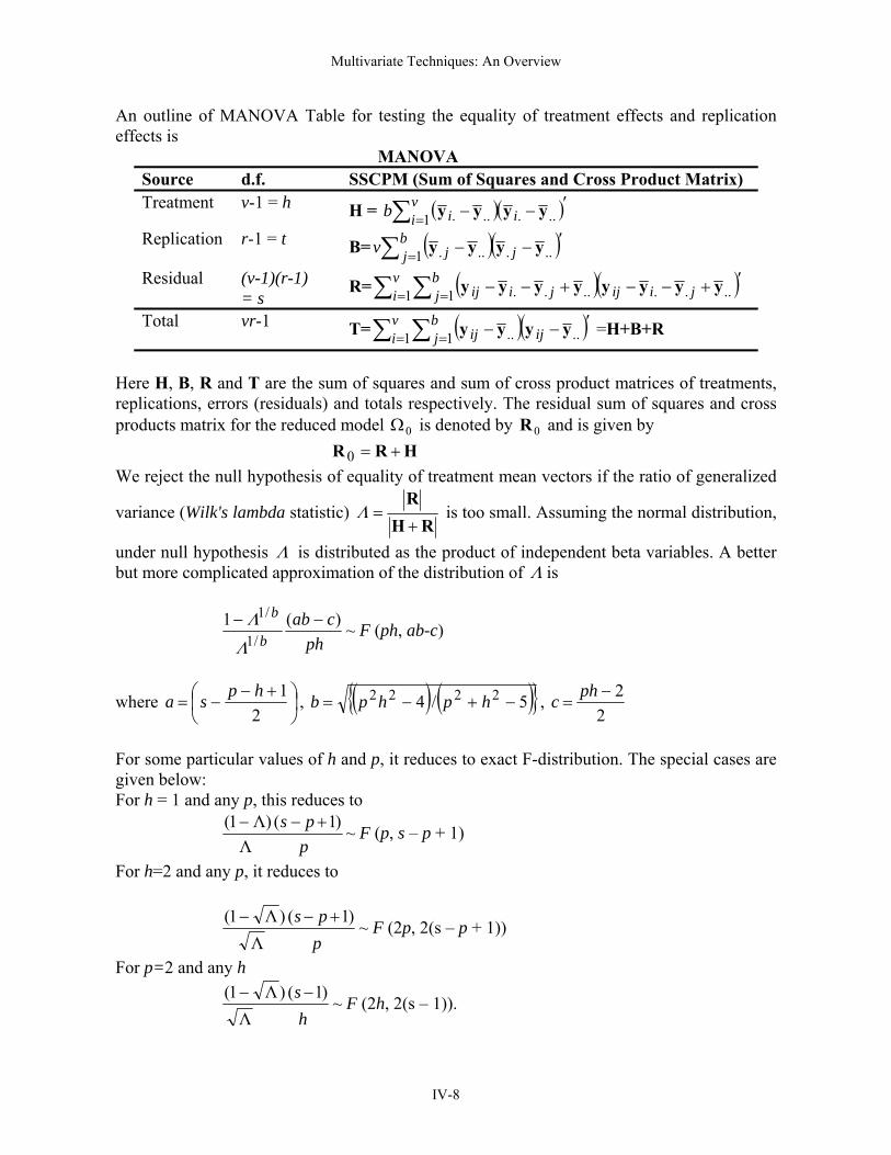
An outline of MANOVA Table for testing the equality of treatment effects and replication effects is

MANOVA Source d.f. SSCPM (Sum of Squares and Cross Product Matrix) Treatment v-1 = h H = ( )( )∑ =

′−−vi iib 1 ...... yyyy

Replication r-1 = t B= ( )( )∑ =′−−b

j jjv 1 ...... yyyy

Residual (v-1)(r-1) = s

R= ( )( )∑ ∑= =′+−−+−−v

ibj jiijjiij1 1 ........ yyyyyyyy

Total vr-1 T= ( )( )∑ ∑= =′−−v

ibj ijij1 1 .... yyyy =H+B+R

Here H, B, R and T are the sum of squares and sum of cross product matrices of treatments, replications, errors (residuals) and totals respectively. The residual sum of squares and cross products matrix for the reduced model 0Ω is denoted by 0R and is given by

HRR +=0 We reject the null hypothesis of equality of treatment mean vectors if the ratio of generalized

variance (Wilk's lambda statistic) RH

R+

=Λ is too small. Assuming the normal distribution,

under null hypothesis Λ is distributed as the product of independent beta variables. A better but more complicated approximation of the distribution of Λ is

phcab

b

b )(1/1

/1 −−

Λ

Λ ~ F (ph, ab-c)

where ⎟⎠⎞

⎜⎝⎛ +−

−=2

1hpsa , ( ) ( ) 5/4 2222 −+−= hphpb , 2

2−=

phc

For some particular values of h and p, it reduces to exact F-distribution. The special cases are given below: For h = 1 and any p, this reduces to

pps

Λ)1(Λ)1( +−− ~ F (p, s – p + 1)

For h=2 and any p, it reduces to

pps

Λ)1()Λ1( +−− ~ F (2p, 2(s – p + 1))

For p=2 and any h

hs

Λ)1()Λ1( −− ~ F (2h, 2(s – 1)).


IV-9

For p = 1, the statistic reduces to the usual variance ratio statistics. The hypothesis regarding the equality of replication effects can be tested by replacing Λ by

RBR+

and h by t in the above.

Remark: One complication of multivariate analysis that does not arise in the univariate case is due to the ranks of the matrices. The rank of R should not be smaller than p or in other words error degrees of freedom s should be greater than or equal to p (s ≥ p). For performing MANOVA using SAS, the following procedures/statements may be used. PROC ANOVA and PROC GLM can be used to perform analysis of variance even for more than one dependent variables. PROC ANOVA performs the analysis of variance for balanced data whereas PROC GLM can analyze both balanced and unbalanced data. As ANOVA takes into account the special features of a balanced data, it is faster and uses less storage than PROC GLM for balanced data. The basic syntax of the ANOVA procedure is as given PROC ANOVA <options>; CLASS Variables; MODEL dependents = independent variables (or effects)/ options; MEANS effects / options, ABSORB Variables; FREQ Variable; TEST H=effects E= effect M = equations/options; REPEATED factor - name levels / options; BY variables; RUN; The PROC ANOVA, CLASS and MODEL statements are must. The other statements are optional. The class statement defines the variables for classification (numeric or character variables - maximum characters = 16). PROC GLM for analysis of variance is similar to PROC ANOVA. The statements listed for PROC ANOVA are also used for PROC GLM. The following more statements can be used with PROC GLM; CONTRAST ‘label’ effect name < .... effect coefficients > / < options>; ESTIMATE ‘label’ effect name < ... effect coefficients / <options>; ID variables; LSMEANS effects </options>; OUTPUT <OUT = SAS-data-set > keyword = names< ... keyword=names; RANDOM effects/ < options > ; WEIGHT; However, if the MODEL statement includes more than one dependent variable, additional multivariate statistics can be requested with the MANOVA statement.


IV-10

When a MANOVA statement appears before the first RUN statement, GLM or ANOVA enters a multivariate mode with respect to the handling of missing values; observations with missing independent or dependent variables are excluded from the analysis. If you want to use this mode of handling missing values and do not need any multivariate analysis, specify the MANOVA option in the PROC GLM statement. If both the CONTRAST and MANOVA statements are to be used, the MANOVA statement must appear after the CONTRAST statement. The basic syntax of MANOVA statement is MANOVA; MANOVA < H=effects INTERCEPT _ALL_ ><E=effect></options>; MANOVA < H=effects INTERCEPT _ALL_><E=effect> <M=equation,...,equation (row-or-matrix,...,row-or-matrix)> <MNAMES=names><PREFIX=name></options>; The terms given in the MANOVA statement are specified as follows: H=effects INTERCEPT _ALL_ : specifies effects in the preceding model to use as hypothesis matrices. For each H matrix (the SSCP matrix associated with that effects), the H=specification prints the characteristic roots and vectors of E-1H ( where E is the matrix associated with the error effects), Hotelling-Lawley trace, Pillai’s trace, Wilks’ criterion, and Roy’s maximum root criterion with approximate F statistic. Use the keyword INTERCEPT to print tests for the intercept. To print tests for all effects listed in the MODEL statement, use the keyword _ALL_ in place of a list of effects. E=effect : specifies the error effect. If we omit the E=specification, GLM uses the error SSCP (residual) matrix from the analysis. <M=equation, ..., equation (row-or-matrix,...,row-or-matrix)> : specifies a transformation matrix for the dependent variables listed in the MODEL statement. The equations in the M=specification are of the form C1

*dependent-variable±C2*dependent-variable ±Cn

*dependent-variable where the Ci values are coefficients for the various dependent-variables. If the value of a given Ci is 1, it may be omitted; in other words, 1*Y is the same as Y. Equations should involve two or more dependent variables. Alternatively, we can input the transformation matrix directly by entering the elements of the matrix with commas separating the rows, and parentheses surrounding the matrix. When this alternate form of input is used, the number of elements in each row must equal the number of dependent variables. Although these combinations actually represent the columns of the M matrix, they are printed by rows. When we include an M=specification, the analysis requested in the MANOVA statement is carried out for the variables defined by the equations in the specification, not the original dependent variables. If M=is omitted, the analysis is performed for the original dependent variables in the MODEL statement. If an M=specification is included without either the MNAMES= or PREFIX=option, the variables are labeled by default as MVAR1, MVAR2, and so on.


IV-11

MNAMES= names : provides names for the variables defined by the equations in the M=specification. Names in the list correspond to the M=equations or the rows of the M matrix (as it is entered). PREFIX = name : is an alternative means of identifying the transformed variables defined by the M=specification. For example, if you specify PREFIX = DIFF, the transformed variables are labeled DIFF1, DIFF2, and so on. The following options can be used in the MANOVA statement CANONICAL : Prints a canonical analysis of the H and E matrices (transformed by the M matrix, if specified) instead of the default printout of characteristic roots and vectors. ETYPE=n : specifies the type(1,2,3, or 4) of the E matrix. By default, the procedure uses an ETYPE=value corresponding to the highest type (largest n ) used in the analysis. HTYPE =n : specifies the type (1,2,3, or 4) of the H matrix. ORTH : requests that the transformation matrix in the M=specification of the MANOVA statement be orthonormalized by rows before the analysis. PRINTE : prints the E matrix. If the E matrix is the error SSCP (residual) matrix from the analysis, the partial correlations of the dependent variables given the independent variables are also printed. For example, the statement

manova / printe;

prints the error SSCP matrix and the partial correlation matrix computed from the error SSCP matrix.

PRINTH : prints the H matrix (the SSCP matrix) associated with each effect specified by the H=specification.

SUMMARY : produces analysis-of-variance tables for each dependent variable. When no M matrix is specified, a table is printed for each original dependent variable from the MODEL statement; with an M matrix other than the identity, a table is printed for each transformed variable defined by the M matrix. Various ways of using a MANOVA statement are given as follows: proc glm; class a b; model y1-y5=a b(a); manova h=a e=b(a) / printh printe htype=1 etype=1; manova h=b(a) / printe; manova h=a e=b(a) m=y1-y2, y2-y3, y3-y4, y4-y5 prefix=diff; manova h=a e=b(a) m=(1 -1 0 0 0, 0 1 -1 0 0, 0 0 1 -1 0,


IV-12

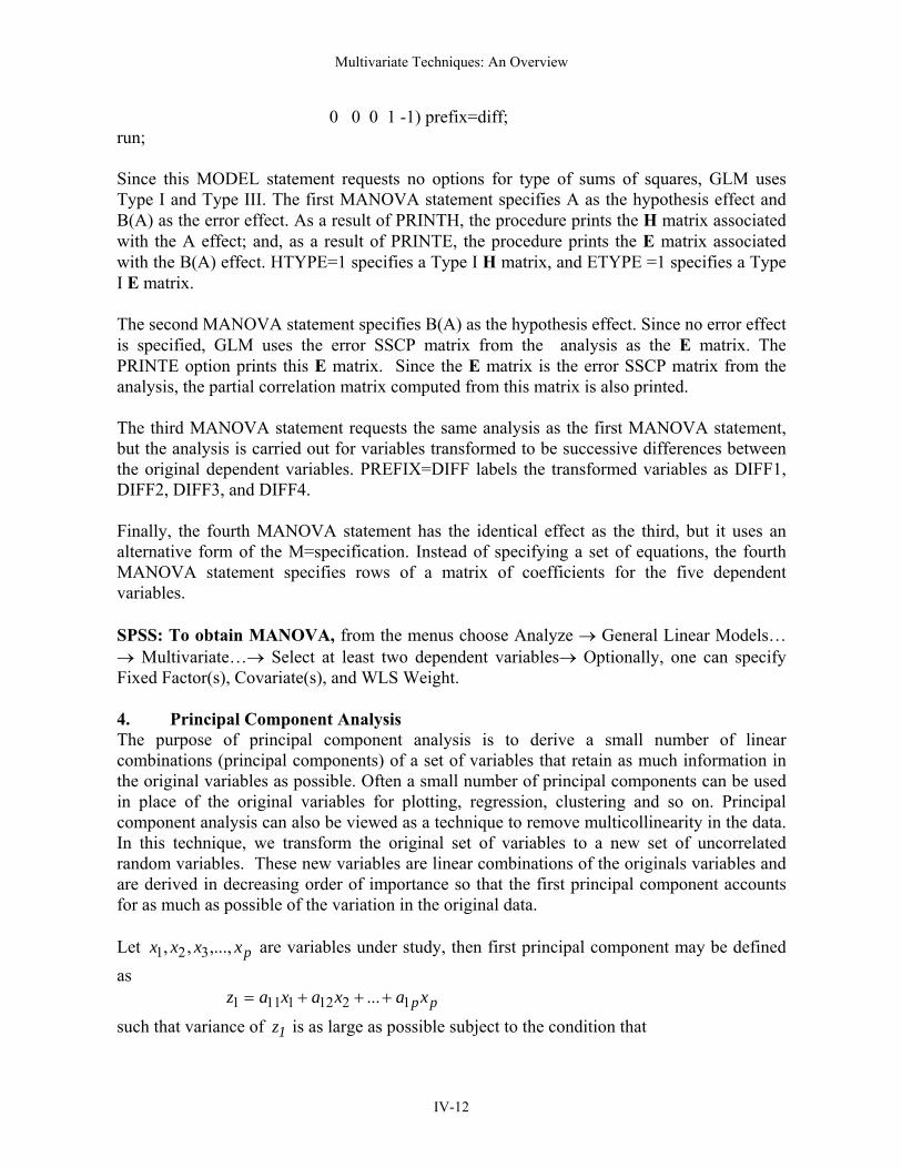
0 0 0 1 -1) prefix=diff; run; Since this MODEL statement requests no options for type of sums of squares, GLM uses Type I and Type III. The first MANOVA statement specifies A as the hypothesis effect and B(A) as the error effect. As a result of PRINTH, the procedure prints the H matrix associated with the A effect; and, as a result of PRINTE, the procedure prints the E matrix associated with the B(A) effect. HTYPE=1 specifies a Type I H matrix, and ETYPE =1 specifies a Type I E matrix. The second MANOVA statement specifies B(A) as the hypothesis effect. Since no error effect is specified, GLM uses the error SSCP matrix from the analysis as the E matrix. The PRINTE option prints this E matrix. Since the E matrix is the error SSCP matrix from the analysis, the partial correlation matrix computed from this matrix is also printed. The third MANOVA statement requests the same analysis as the first MANOVA statement, but the analysis is carried out for variables transformed to be successive differences between the original dependent variables. PREFIX=DIFF labels the transformed variables as DIFF1, DIFF2, DIFF3, and DIFF4. Finally, the fourth MANOVA statement has the identical effect as the third, but it uses an alternative form of the M=specification. Instead of specifying a set of equations, the fourth MANOVA statement specifies rows of a matrix of coefficients for the five dependent variables. SPSS: To obtain MANOVA, from the menus choose Analyze → General Linear Models… → Multivariate…→ Select at least two dependent variables→ Optionally, one can specify Fixed Factor(s), Covariate(s), and WLS Weight. 4. Principal Component Analysis The purpose of principal component analysis is to derive a small number of linear combinations (principal components) of a set of variables that retain as much information in the original variables as possible. Often a small number of principal components can be used in place of the original variables for plotting, regression, clustering and so on. Principal component analysis can also be viewed as a technique to remove multicollinearity in the data. In this technique, we transform the original set of variables to a new set of uncorrelated random variables. These new variables are linear combinations of the originals variables and are derived in decreasing order of importance so that the first principal component accounts for as much as possible of the variation in the original data. Let pxxxx ,...,,, 321 are variables under study, then first principal component may be defined as ppxaxaxaz 12121111 ...+++=

such that variance of 1z is as large as possible subject to the condition that


IV-13

1... 21

212

211 =+++ paaa

This constraint is introduced because if this is not done, then ( )1zVar can be increased simply by multiplying any sa j '1 by a constant factor. The second principal component is defined as

ppxaxaxaz 22221212 ...+++=

such that ( )2zVar is as large as possible next to ( )1zVar subject to the constraint that

1... 22

222

221 =+++ paaa and ( ) 0, 21 =zzCov and so on.

It is quite likely that first few principal components account for most of the variability in the original data. If so, these few principal components can then replace the initial p variables in subsequent analysis, thus reducing the effective dimensionality of the problem. An analysis of principal components often reveals relationships that were not previously suspected and thereby allows interpretation that would not ordinarily result. However, Principal Components Analysis is more of a mean to an end rather than end in itself because this frequently serves as intermediate steps in much larger investigations by reducing the dimensionality of the problem and providing easier interpretation. It is a mathematical technique, which does not require user to specify the statistical model or assumption about distribution of original variates. It may also be mentioned that principal components are artificial variables and often it is not possible to assign physical meaning to them. Further, since Principal Components Analysis transforms original set of variables to new set of uncorrelated variables. It is worth stressing that if the original variables are uncorrelated, then there is no point in carrying out the Principal Components Analysis. It is important to note here that the principal components depend on the scale of measurement. Conventional way of getting rid of this problem is to use the standardized variables with unit variances. Example 4: Let us consider the following data on average minimum temperature ( )1x , average relative humidity at 8 hrs. ( )2x , average relative humidity at 14 hrs. ( )3x and total rainfall in cm. ( )4x pertaining to Raipur district from 1970 to 1986 for kharif season from 21st May to 7th Oct. x1 x2 x3 x4 25.0 86 66 186.49 24.9 84 66 124.34 25.4 77 55 98.79 24.4 82 62 118.88 22.9 79 53 71.88 7.7 86 60 111.96 25.1 82 58 99.74 24.9 83 63 115.20 24.9 82 63 100.16 24.9 78 56 62.38 24.3 85 67 154.40


IV-14

24.6 79 61 112.71 24.3 81 58 79.63 24.6 81 61 125.59 24.1 85 64 99.87 24.5 84 63 143.56 24.0 81 61 114.97 Mean 23.56 82.06 61.00 112.97 S.D. 4.13 2.75 3.97 30.06 with the variance co-variance matrix.

∑⎥⎥⎥⎥

⎦

⎤

⎢⎢⎢⎢

⎣

⎡ −

=

87.90395.9275.1582.5450.856.714.554.112.402.17

Find the eigenvalues and eigenvectors of the above matrix. Arrange the eigenvalues in decreasing order. Let the eigenvalues in decreasing order and corresponding eigenvectors are

( )993.0,103.0,061.0,006.0902.9161 == 1aλ ( )012.0,011.0,296.0,955.0375.182 −== 2aλ ( )119.0,855.0,485.0,141.087.73 −== 3aλ ( )001.0,509.0,820.0,260.0056.14 −== 4aλ

The principal components for this data will be

43214

43213

43212

43211

001.0509.082.026.0119.0855.0485.0141.0012.0011.0296.0955.0993.0103.0061.0006.0

xxxxzxxxxzxxxxzxxxxz

+−+=−++=

++−=+++=

The variance of principal components will be eigenvalues i.e.

( ) ( ) ( ) ( ) 056.1,87.7,375.18,902.916 4321 ==== zVarzVarzVarzVar The total variation explained by principal components is

20.944056.187.7375.18902.9164321 =+++=+++ λλλλ As such, it can be seen that the total variation explained by principal components is same as that explained by original variables. It could also be proved mathematically as well as empirically that the principal components are uncorrelated. The proportion of total variation accounted for by the principal components is

97.0203.944902.916

43211 ==

+++ λλλλλ

Continuing, the first two components account for a proportion


IV-15

99.0203.944277.935

432121 ==+++

+λλλλ

λλ

of the total variance. Hence, in further analysis, the first or first two principal components 1z and 2z could replace four variables by sacrificing negligible information about the total variation in the system. The scores of principal components can be obtained by substituting the values of ix 's in the equations of iz 's. For above data, the first two principal components for first observation i.e. for year 1970 can be worked out as

383.149.186012.066011.086296.00.25955.0380.19749.186993.066103.086061.00.25006.0

2

1=×+×+×−×==×+×+×+×=

zz

Similarly for the year 1971

134.134.124012.066011.084296.09.24955.054.13534.124993.066103.084061.09.24006.0

2

1=×+×+×−×==×+×+×+×=

zz

Thus the whole data with four variables can be converted to a new data set with two principal components. Example 5: Consider the same data as given in Example 1. The variance-covariance matrix was given as

⎥⎥⎥

⎦

⎤

⎢⎢⎢

⎣

⎡

−−−

−=

627658.364.580905.164.57884.19901.10

80905.101.10879368.2Σ

Now find the eigenvalues and eigenvectors of the above matrix. Arrange the eigenvalues in decreasing order. Let the eigenvalues in decreasing order and corresponding eigenvectors are

( )0291.0,9983.0,0508.0462.2001 −== 1aλ ( )8173.0,0530.0,5737.0532.42 −== 2aλ ( )5754.0,0249.0,8175.0301.13 −== 3aλ

The principal components for this data are

3213

3212

3211

5754.00249.08175.08173.00530.05737.0

0291.09983.00508.0

xxxzxxxz

xxxz

+−=++−=

−+=

The variance of principal components will be eigenvalues i.e.

( ) ( ) ( ) 301.1,532.4,462.200 321 === zVarzVarzVar The total variation explained by principal components is

295.206301.1532.4462.200321 =++=++ λλλ


IV-16

As such, it can be seen that the total variation explained by principal components is same as that explained by original variables. It could also be proved mathematically as well as empirically that the principal components are uncorrelated. The proportion of total variation accounted for by the principal components is

9717.0295.206462.200

321

1 ==++ λλλ

λ of the total variance.

Continuing, the first two components account for a proportion

9937.0295.206994.204

321

21 ==++

+λλλ

λλ of the total variance.

Hence, in further analysis, the first or first two principal components 1z and 2z could replace four variables by sacrificing negligible information about the total variation in the system. The scores of principal components can be obtained by substituting the values of ix 's in the equations of iz 's. For above data, the first two principal components for first observation i.e. for first individual is

3.98173.05.480530.07.35737.03.90291.05.489983.07.30508.0

2

1×+×+×−=

×−×+×=zz

Similarly principal component scores for other individuals can be obtained. Thus the whole data with three variables can be converted to a new data set with two principal components. Following steps of SAS may be used for performing the principal component analysis. The PROC PRINCOMP can be used for performing principal component analysis. Raw data, a correlation matrix, a covariance matrix or a sum of squares and cross products (SSCP) matrix can be used as input data. The data sets containing eigenvalues, eigenvectors, and standardized or unstandardized principal component scores can be created as output. The basic syntax of PROC PRINCOMP is as follows: PROC PRINCOMP <options>; BY variables; FREQ Variable; PARTIAL Variables; VAR Variables; WEIGHT Variable; RUN; The PROC PRINCOMP and RUN are must. However, the VAR statement listing the numeric variables to be analysed is usually used alongwith PROC PRINCOMP statement. If the DATA= data set is TYPE=SSCP, the default set of variables does not include intercept.


IV-17

Therefore, INTERCEPT may also be included in the VAR statement. The following options are available in PROC PRINCOMP. A. DATA SETS SPECIFICATION 1. DATA= SAS-data-set : names the SAS data set to be analysed. This data set can be

ordinary data set or a TYPE = CORR, COV, FACTOR, UCORR or UCOV data set. 2. OUT = SAS-data-set : creates an output data set containing original data alongwith

principal component scores. 3. OUTSTAT-SAS-data-set : creates an output data set containing means, standard

deviations, number of observations, correlations or covariances, eigenvalues and eigenvectors.

B. ANALYTICAL DETAILS SPECIFICATION 1. COV: computes the principal components from the covariance matrix. The default option

is computation of principal components using a correlation matrix. 2. N=: the non-negative integer equal to the number of principal components to be

computed. 3. NOINT : omits the intercept from the model 4. PREFIX= name: specifies a prefix for naming the principal components. The default

option is PRIN1, PRIN2, ... . 5. STANDARD (STD): standardizes the principal component scores to unit variance from

the variance equal to corresponding eigenvalue. 6. VARDEF=DFNWDFWEIGHT: specifies the divisor (error degree of

freedomnumber of observationssun of weightssum of weights-1) in calculating variances and standard deviations. The default option is DF.

Besides these options NOPRINT option suppresses the output. The other statements in PROC PRINCOMP are: By variables: obtains the separate analysis on observations in groups defined by variables. FREQ statement: It names a variable that provides frequencies of each observation in the data set. Specifically, if n is the value of the FREQ variable for a given observation, then that observation is used ‘n’ times. PARTIAL Statement: used to analyze for a partial correlation or covariance matrix. VAR statement: Lists the numeric variables to be analysed. WEIGHT Statement: If we want to use relative weights for each observation in the input data set, place the weights in a variable in the data set and specify the name in a weight statement. This is often done when the variance associated with each observation is different and the values of the weight variable are proportional to reciprocals of the variances. The observation is used in the analysis only if the value of the WEIGHT statement variable is non-missing and greater than zero.


IV-18

The other closely related procedures with PROC PRINCOMP are PROC PRINQUAL: It performs a principal component analysis of a qualitative data. PROC CORRESP: performs correspondence analysis, which is a weighted principal component analysis of contingency tables. 5. Canonical Correlation Analysis Canonical correlation is a technique for analyzing the relationship between two sets of variables. Each set can contain several variables. Simple and multiple correlation are special cases of canonical correlation in which one or both sets contain a single variable. This analysis actually focuses on the correlation between a linear combination of the variables in one set and a linear combination of the variables in the second set. The idea is first to determine the pair of linear combinations having the largest correlation. Next we determine the pair of linear combinations having the largest correlation among all pairs uncorrelated with the initially selected pair. This process continues until the number of pairs of canonical variables equals the number of variables in the smaller group. The pairs of linear combinations are called the canonical variables and their correlations are called canonical correlations. The canonical correlations measure the strength of association between the two sets of variables. The maximization aspect of the technique represents an attempt to concentrate a high-dimensional relationship between two sets of variables into a few pair of canonical variables. The PROC CANCORR procedure tests a series of hypotheses that each canonical correlation and all smaller correlations are zero in population using an F-approximation. At least one of the two sets of the variables should have an approximate multivariate normal distribution. PROC CANCORR can also perform partial canonical correlation, a multivariate generalization of ordinary partial correlation. Most commonly used parametric statistical methods, ranging from t-tests to multivariate analysis of covariance are special cases of partial canonical correlations. 6. Discriminant Analysis The term discriminant analysis refers to several types of analysis viz. classificatory discriminant analysis (used to classify observations into two or more known groups on the basis of one or more quantitative variables), Canonical discriminant analysis (a dimension reduction technique related to principal components and canonical correlation), Stepwise discriminant analysis (a variable selection technique i.e. to try to find a subset of quantitative variables that best reveals differences among the classes). For classificatory discriminant analysis, Fisher's Discriminant function is generally used. It is described in the sequel. Fisher's idea was to transform the multivariate observations x to univariate observations y such the y's derived from the populations 1π and 2π were separated as much as possible. Fisher's approach assumes that the populations are normal and also assumes the population covariance matrices are equal because a pooled estimate of common covariance matrix is used.


IV-19

A fixed linear combination of the x's takes the values

111211 ,....,, nyyy for the observations

from the first population and the values 222221 ,....,, nyyy for the observations from the

second population. The separation of these two sets of univariate y's is assessed in terms of the differences between 1y and 2y expressed in standard deviation units. That is,

ysyy 21nseparartio

−= , where

( ) ( )221

1

222

1

211

2

21

−+

−+−

=∑∑==

nn

yyyy

s

n

jj

n

jj

y

is the pooled estimate of the variance. The objective is to select the linear combination of the x to achieve maximum separation of the sample means 1y and 2y . Result: The linear combination ( ) xSxxxl 1

21ˆ −′−=′= pooledy maximizes the ratio

( )( )yofvarianceSample

yofmeansamplebetweendistanceSquared ( )2

221

ysyy −

=

( )Il

xlxlˆˆ

ˆˆ 221

pooledS′′−

=

( )ll

dl′′

′= ˆˆ

ˆ 2

pooledS

over all possible coefficient vectors l′ˆ where ( )21 xxd −= . The maximum of the above ratio

is ( ) ( )211

212 xxSxxD −′−= −

pooled , the Mahalanobis distance. Fisher's solution to the separation problem can also be used to classify new observations. An allocation rule is as follows.

Allocate 0x to 1π if ( ) ( ) ( )211

2101

210 21ˆ xxSxxmxSxx +′−=≥′−= −−

pooledpooledy

and to 2π if m0 <y If we assume the populations 1π and 2π are multivariate normal with a common covariance matrix, the a test of 210 : µµ =H versus 211 : µµ ≠H is accomplished by referring ( )( )

2

21

21

21

212

1 D⎟⎟⎠

⎞⎜⎜⎝

⎛+−+

−−+nn

nnpnn

pnn


IV-20

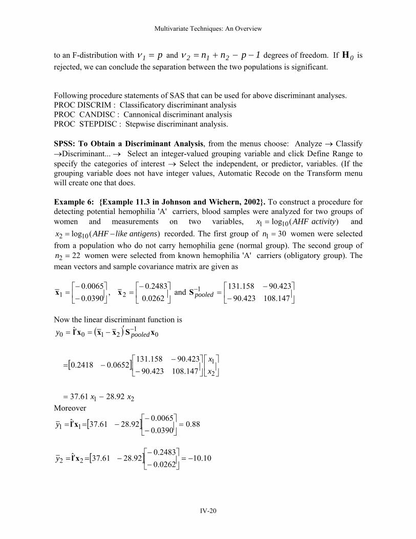
to an F-distribution with p1 =ν and 1pnn 212 −−+=ν degrees of freedom. If 0H is rejected, we can conclude the separation between the two populations is significant. Following procedure statements of SAS that can be used for above discriminant analyses. PROC DISCRIM : Classificatory discriminant analysis PROC CANDISC : Cannonical discriminant analysis PROC STEPDISC : Stepwise discriminant analysis. SPSS: To Obtain a Discriminant Analysis, from the menus choose: Analyze → Classify →Discriminant... → Select an integer-valued grouping variable and click Define Range to specify the categories of interest → Select the independent, or predictor, variables. (If the grouping variable does not have integer values, Automatic Recode on the Transform menu will create one that does. Example 6: Example 11.3 in Johnson and Wichern, 2002. To construct a procedure for detecting potential hemophilia 'A' carriers, blood samples were analyzed for two groups of women and measurements on two variables, )(log101 activityAHFx = and

)(log102 antigenslikeAHFx −= recorded. The first group of 301 =n women were selected from a population who do not carry hemophilia gene (normal group). The second group of

222 =n women were selected from known hemophilia 'A' carriers (obligatory group). The mean vectors and sample covariance matrix are given as

⎥⎦

⎤⎢⎣

⎡−−

=0390.00065.0

1x , ⎥⎦

⎤⎢⎣

⎡−=

0262.02483.0

2x and ⎥⎦

⎤⎢⎣

⎡−

−=−

147.108423.90423.90158.1311

pooledS

Now the linear discriminant function is

( )

[ ]

21

2

1

01

2100

92.2861.37

147.108423.90423.90158.131

0652.02418.0

ˆ

xx

xx

y pooled

−=

⎥⎦

⎤⎢⎣

⎡⎥⎦

⎤⎢⎣

⎡−

−−=

′−=′= − xSxxxl

Moreover

[ ] 88.00390.00065.0

92.2861.37ˆ 11 =⎥⎦

⎤⎢⎣

⎡−−

−=′= xly

[ ] 10.100262.02483.0

92.2861.37ˆ 22 −=⎥⎦

⎤⎢⎣

⎡−−

−=′= xly


IV-21

And the mid-point between these means is

( ) ( ) ( ) 61.421

21ˆ 2121

121 −=+=+′−= − yypooled xxSxxm

Now to classify a women who may be a hemophilia 'A' carrier with 210.01 −=x and

044.02 −=x . We calculate: 62.692.2861.37ˆ 2100 −=−=′= xxy xl . Since m0 <y we classify the women in 2π population, i.e., to obligatory carrier group. 7. Factor Analysis The essential purpose of factor analysis is to describe, if possible, the covariance relationships among many variables in terms of a few underlying but unobservable random quantities called factors. A frequent source of confusion in the field of factor analysis is the term factor. It sometimes refers to a hypothetical, unobservable variable as in the phrase common factor. In this sense, factor analysis must be distinguished from component analysis since a component is an observable linear combination. Factor is also used in the sense of matrix factor, in that one matrix is a factor of second matrix if the first matrix multiplied by its transpose equals the second matrix. In this sense, factor analysis refers to all methods of data analysis using matrix factors, including component analysis and common factor analysis. A common factor is an unobservable hypothetical variable that contributes to that variance of at least two of the observed variables. The unqualified term “ factor” often refers to a common factor. A unique factor is an unobservable hypothetical variable that contributes to the variance of only one of the observed variables. The model for common factor analysis posits one unique factor for each observed variable. The PROC FACTOR can be used for several types of common factor and component analysis. Both orthogonal and oblique rotations are available. We can compute scoring coefficients by the regression method. All major statistics computed by PROC FACTOR can also be saved in an output DATA SET. The PROC FACTOR can be invoked by the following statements: PROC FACTOR <options>; VAR variables; PRIORS Communalities; PARTIAL Variables; FREQ Variable; WEIGHT Variable; BY variables; RUN; Usually only the VAR statement is needed in addition to the PROC FACTOR statement. The some of the important options available with PROC FACTOR are: METHOD=NAME : specifies the method of extracting factors. The default option is METHOD = PRINCIPAL, which yields principal component analysis if no PRIORS is used


IV-22

or if PRIORS = ONE is specified; if a PRIORS = value other than one is specified, a principal factor anlaysis is performed. METHOD= PRINT : yields iterated principal factor analysis. METHOD=ML : performs maximum- likelihood factor analysis. METHOD = ALPHA : produced alpha factor analysis. METHOD =ULS: produced unweighted least squares factor anlaysis. NFACTORS=nNFACT=nN=n specifies the maximum number of factors to be extracted. PRIORS =name: (ASMCINPUTMAXONERANDOMSMC) : specifies a method for computing prior communality estimates ROTATE=name: gives the rotation method. The default is ROTATE=NONE. FACTOR performs the following orthogonal rotation methods: • EQUAMAX • ORTHOMAX • QUARTIMAX • PARSIMAX • VARIMAX After the initial factor extraction, the common factors are uncorrelated with each other. If the factors are rotated by an orthogonal transformation, the rotated factors are uncorrelated. If the factors are rotated by an oblique transformation, the rotated factors become correlated. Oblique rotations often produce more useful patterns than do orthogonal rotations. However, a consequence of correlated factors is that there is no single unambiguous measure of the importance of a factor in explaining a variable. Thus, for oblique rotations, the pattern matrix doesn’t provide all the necessary information for interpreting the factors. SPSS: To Perform Factor Analysis. From the menus choose: Analyze → Data Reduction → Factor... → Select the variables for the factor analysis. To understand the role of Factor Analysis, consider the following examples Example 7: What underlying attitudes lead people to respond to the questions on a political survey as they do? Examining the correlations among the survey items reveals that there is significant overlap among various subgroups of items--questions about taxes tend to correlate with each other, questions about military issues correlate with each other, and so on. With factor analysis, you can investigate the number of underlying factors and, in many cases, you can identify what the factors represent conceptually. Additionally, you can compute factor scores for each respondent, which can then be used in subsequent analyses. For example, you might build a logistic regression model to predict voting behavior based on factor scores.

Example 8: A manufacturer of fabricating parts is interested in identifying the determinants of a successful salesperson. The manufacturer has on file the information shown in the


IV-23

following table. He is wondering whether he could reduce these seven variables to two or three factors, for a meaningful appreciation of the problem.

Data Matrix for Factor Analysis of seven variables (14 sales people)

Sales Person

Height ( )1x

Weight( )2x

Education( )3x

Age( )4x

No. of Children

( )5x

Size of Household

( )6x

IQ( )7x

1 67 155 12 27 0 2 102 2 69 175 11 35 3 6 92 3 71 170 14 32 1 3 111 4 70 160 16 25 0 1 115 5 72 180 12 36 2 4 108 6 69 170 11 41 3 5 90 7 74 195 13 36 1 2 114 8 68 160 16 32 1 3 118 9 70 175 12 45 4 6 121 10 71 180 13 24 0 2 92 11 66 145 10 39 2 4 100 12 75 210 16 26 0 1 109 13 70 160 12 31 0 3 102 14 71 175 13 43 3 5 112 Can we now collapse the seven variables into three factors? Intuition might suggest the presence of three primary factors: maturity revealed in age/children/size of household, physical size as shown by height and weight, and intelligence or training as revealed by education and IQ. The sales people data have been analyzed by the SAS program. This program accepts data in the original units, automatically transforming them into standard scores. The three factors derived from the sales people data by principal component analysis (SAS program) are presented below:


IV-24

Three-factor results with seven variables Sales People Characteristics

Variable Factor I Factor II Factor III

Communality Height 0.59038 0.72170 -0.30331 0.96140 (sumsq I,II

and III) Weight 0.45256 0.75932 -0.44273 0.97738 Education 0.80252 0.18513 0.42631 0.86006 Age -0.86689 0.41116 0.18733 0.95564 No. of Children

-0.84930 0.49247 0.05883 0.96730

Size of Household

-0.92582 0.30007 -0.01953 0.94756

IQ 0.28761 0.46696 0.80524 0.94918 Sum of squares

3.61007 1.85136 1.15709

Variance summarized

0.51572 0.26448 0.16530 Average=0.94550

Factor Loadings The coefficients in the factor equations are called "factor loadings". They appear above in each factor column, corresponding to each variable. The equations are:

76543211 28761.092582.084930.086689.080252.045256.059038.0 xxxxxxx +−−−++=F

76543212 46696.030007.049247.041116.018513.075932.072170.0 xxxxxxx ++++++=F

76543213 80524.001953.058830.018733.080252.044273.030331.0 xxxxxxx +−+++−−=F The factor loadings depict the relative importance of each variable with respect to a particular factor. In all the three equations, education ( )3x and IQ ( )7x have got positive loading factor indicating that they are variables of importance in determining the success of sales person. Variance summarized Factor analysis employs the criterion of maximum reduction of variance - variance found in the initial set of variables. Each factor contributes to reduction. In our example Factor I accounts for 51.6% of the total variance. Factor II for 26.4% and Factor III for 16.5%. Together the three factors "explain" almost 95% of the variance. Communality In the ideal solution the factors derived will explain 100% of the variance in each of the original variables, "Communality" measures the percentage of the variance in the original variables that is captured by the combinations of factors in the solution. Thus communality is computed for each of the original variables. Each variables communality might be thought of as showing the extent to which it is revealed by the system of factors. In our example the communality is over 85% for every variable. Thus the three factors seem to capture the underlying dimensions involved in these variables.


IV-25

There is yet another analysis called varimax rotation, after we get the initial results. This could be employed if needed by the analyst. We do not intend to dwell on this and those who want to go into this aspect can use SAS program for varimax rotation. 8. Cluster Analysis The basic aim of the cluster analysis is to find “natural” or “real” groupings, if any, of a set of individuals (or objects or points or units or whatever). This set of individuals may form a complete population or be a sample from a larger population. More formally, cluster analysis aims to allocate a set of individuals to a set of mutually exclusive, exhaustive groups such that individuals within a group are similar to one another while individuals in different groups are dissimilar. This set of groups is called partition or dissection. Cluster analysis can also be used for summarizing the data rather than finding natural or real groupings. Grouping or clustering is distinct from the classification methods in the sense that the classification pertains to a known number of groups, and the operational objective is to assign new observations to one of these groups. Cluster analysis is a more primitive technique in that no assumptions are made concerning the number of groups or the group structure. Grouping is done on the basis of similarities or distances (dissimilarities). Some of these distance criteria are: Euclidean distance: This is probably the most commonly chosen type of distance. It is the geometric distance in the multidimensional space and is computed as:

)()()(),(2/1

1

2 yxyxyx −′−=⎥⎥⎦

⎤

⎢⎢⎣

⎡−= ∑

=

p

iii yxd

where yx, are the p-dimensional vectors of observations. Note that Euclidean (and squared Euclidean) distances are usually computed from raw data, and not from standardized data. This method has certain advantages (e.g., the distance between any two objects is not affected by the addition of new objects to the analysis, which may be outliers). However, the distances can be greatly affected by differences in scale among the dimensions from which the distances are computed. For example, if one of the dimensions denotes a measured length in centimeters, and you then convert it to millimeters (by multiplying the values by 10), the resulting Euclidean or squared Euclidean distances (computed from multiple dimensions) can be greatly affected (i.e., biased by those dimensions which have a larger scale), and consequently, the results of cluster analyses may be very different. Generally, it is good practice to transform the dimensions so they have similar scales. Squared Euclidean distance: This measure is used in order to place progressively greater weight on objects that are further apart. This distance is square of the Euclidean distance. Statistical distance: The statistical distance between the two p-dimensional vectors yx and

is )()()( 1 yxsyxyx, −′−= −d , where s is the sample variance-covariance matrix.


IV-26

Many more distance measures are available in literature. For details, a reference may be made to Romesburg (1984). Several types of clusters are possible using various PROC statements: • Disjoint cluster place each object in one and only one cluster. (PROC FASTCLUS, PROC

VARCLUS). • Hierarchical clusters are organised so that one cluster may be entirely contained within

another cluster, but no other kind of overlap between clusters is allowed. (PROC CLUSTER, PROC VARCLUS).

• Overlapping clusters can be constrained to limit the number of objects that belongs simultaneously to two clusters. (PROC OVERCLUS)

• Fuzzy clusters are defined by a probabilities or grade of membership of each object in each cluster. Fuzzy clusters can be disjoint, hierarchical or overlapping.

SPSS: To Obtain a Hierarchical Cluster Analysis, from the menus choose: Analyze → Classify → Hierarchical Cluster... → For clustering cases, select at least one numeric variable, For clustering variables, select at least three numeric variables → Optionally, one can select an identification variable to label cases. References Johnson, R.A. and Wichern, D.W. (2002). Applied multivariate statistical analysis. 5th

Edition, Pearson Education Inc., New Delhi. Romesburg, H.C. (1984). Cluster Analysis for Researchers. Lifetime Learning Publications,

California.

multivariate techniques: an overview - iasri

Documents