muse-4 experiment measurements and analysis muse-4 experiment measurements and analysis gerardo...
TRANSCRIPT
ANL-AFCI-092
MUSE-4 Experiment Measurements and Analysis
Gerardo Aliberti, George Imel, Giuseppe Palmiotti
Argonne National Laboratory
Nuclear Engineering Division
Argonne National Laboratory
9700 S. Cass Avenue
Argonne, IL 60439
September 2003

September 2003 ANL-AFCI-092
-i-
MUSE-4 Experiment Measurements and Analysis
Gerardo Aliberti, George Imel, Giuseppe Palmiotti
Argonne National Laboratory
Abstract
This report presents a review of the activities performed by the five teams involved in the MUSE-4 experimental
program. More details are provided on the contribution by ANL during the year 9/02 to 9/03. The ANL activity
consisted both in direct participation in the experimental measurements and in the physics analysis of the
experimental data, mainly for the reactivity level, adjoint flux and fission rate distributions and the analysis of
dynamic measurements for reactivity determination techniques in subcritical systems. The results provided to
complete the Benchmark organized by the OECD and the CEA on the experiment MUSE-4 are also presented.
Deterministic calculations have been performed via the ERANOS code system in connection with JEF2.2,
ENDF/B-V and ENDF/B-VI data files.
Results reported in the AAA series of technical memoranda frequently are preliminary in nature and subject to
revision. Consequently, they should not be quoted or referenced without the author’s permission.

September 2003 ANL-AFCI-092
-ii-
Table of Contents
GLOSSARY.............................................................................................................................................................1
SUMMARY .............................................................................................................................................................2
I. INTRODUCTION................................................................................................................................................3
II. EXPERIMENTAL PROGRAM AND MEASUREMENT TECHNIQUES .......................................................5
II.A. MUSE-4 experiment main events ................................................................................................................5
II.B. The GENEPI accelerator ..............................................................................................................................6
II.B.1. The GENEPI operation ..........................................................................................................................6
II.B.2. Neutron Source Absolute Calibration ....................................................................................................7
II.B.3. Description of measurement acquisition systems ..................................................................................8
II.C. Generalities on standard CEA monitors and detectors used for the measurements at MASURCA...........11
II.C.1. The monitors ........................................................................................................................................11
II.C.2. The experimental fission chambers......................................................................................................12
II.C.3. The CFUK09 chambers .......................................................................................................................13
II.D. Measurement techniques ............................................................................................................................13
II.D.1. Safety measurements ...........................................................................................................................13
II.D.2. Physical measurements ........................................................................................................................13
II.E. The MUSE-4 core configurations...............................................................................................................16
II.E.1. Experimental phase planning ...............................................................................................................16
II.E.2. Main measurements performed on the various configurations ............................................................17
III. CALCULATIONS IN SUPPORT OF THE MUSE-4 PROJECT....................................................................31
III.A. Reactivity measurement and calculation...................................................................................................31
III.A.1. MUSE-4 reference configuration .......................................................................................................34
III.A.2. MUSE-4 SC0 reference configuration ...............................................................................................39
III.A.3. MUSE-4 SC0 reference configuration with bc1 inserted...................................................................41
III.B. Adjoint flux measurement and calculation................................................................................................43
III.B.1. Use of the ECCO code in conjunction with the JEF2.2 data. .............................................................49
III.B.2. Use of the MC2-2 code in conjunction with the ENDF/B-V data.......................................................50
III.B.3. Use of the MC2-2 code in conjunction with the ENDF/B-VI data. ....................................................51
III.B.4. Use of the MC2-2 code in conjunction with the JEF2.2 data..............................................................52
III.B.5. Effect due to the nuclear data on the adjoint flux traverses. ...............................................................53
III.C. Reaction rate traverses measurement and calculation. ..............................................................................54
III.C.1. Use of the ECCO code in conjunction with the ECCO data. .............................................................55
III.C.2. Use of the MC2-2 code in conjunction with the ENDF/B-V data.......................................................56
III.C.3. Use of the MC2-2 code in conjunction with the ENDF/B-VI data. ....................................................57
September 2003 ANL-AFCI-092
-iii-
III.C.4. Use of the MC2-2 code in conjunction with the JEF2.2 data..............................................................58
III.C.5. Effect due to the nuclear data on the adjoint flux traverses. ...............................................................59
III.D. Analysis of dynamic measurements..........................................................................................................60
III.D.1. MUSE-4 SC0 with pilot rod out.........................................................................................................60
III.D.2. MUSE-4 SC0 with pilot rod in...........................................................................................................63
III.D.3. MUSE-4 SC0 with pilot rod and control rod bc1 in...........................................................................65
III.D.4. The use of the PNS methods to infer the reactivity from the analysis of dynamic measurements.....66
IV. MUSE-4 BENCHMARK.................................................................................................................................69
IV.A. Introduction...............................................................................................................................................69
IV.B. Geometry and material description. ..........................................................................................................69
IV.C. Requested calculations..............................................................................................................................74
IV.C.1. COSMO calculations..........................................................................................................................74
IV.C.2 Critical MUSE-4 reference configuration calculations .......................................................................75
IV.C.3. Subcritical configuration calculations ................................................................................................75
IV.D. Calculations details. ..................................................................................................................................76
IV.E. MUSE-4 benchmark revised calculations .................................................................................................78
IV.E.1. Reactivity results ................................................................................................................................78
IV.E.2. Dynamic results ..................................................................................................................................82
APPENDIX A: MC2-2 INCONSISTENCY IN PN APPROXIMATION AND ITS IMPACT ON REFLECTOR
EFFECTS ...............................................................................................................................................................91
I. Introduction .....................................................................................................................................................91
II. Reflector effects study....................................................................................................................................91
III. Theoretical approach.....................................................................................................................................93
IV. Conclusions ..................................................................................................................................................95
APPENDIX B: METHODS FOR INTERFACE CORE/REFLECTOR EFFECTS TREATMENT .....................97
I. Iterative method...............................................................................................................................................97
II. Macrocell method...........................................................................................................................................98
II.1. Standard ECCO calculation...................................................................................................................102
II.2. Standard macrocell calculation..............................................................................................................105
II.3. Improved macrocell calculation ............................................................................................................107
II.4. Perturbation calculation. ........................................................................................................................108
II.5. Application of the improved macrocell option to a 2D model. .............................................................115
REFERENCES.....................................................................................................................................................128

September 2003 ANL-AFCI-092
-iv-
List of Figures
Figure 1: IRI system ...............................................................................................................................................10
Figure 2: Position of the safety rods n°1 and 2 in the core.....................................................................................17
Figure 3: MUSE-4 Critical Reference Configuration – View XY .........................................................................18
Figure 4: MUSE-4 Reference Configuration – View XZ.......................................................................................19
Figure 5: MUSE-4 Reference Configuration – View YZ.......................................................................................19
Figure 6: MUSE-4 Reference Configuration 1114 Cells .......................................................................................20
Figure 7: MUSE-4 Reference Configuration 1119 Cells .......................................................................................21
Figure 8: MUSE-4 Reference Configuration 1114 Cells .......................................................................................22
Figure 9: MUSE-4 SC0 Configuration 1086 Cells.................................................................................................23
Figure 10: MUSE-4 Reference Configuration 1115 Cells .....................................................................................24
Figure 11: MUSE-4 Reference Configuration 1115 Cells .....................................................................................25
Figure 12: MUSE-4 Reference Configuration 1115 Cells .....................................................................................26
Figure 13: MUSE-4 Reference Configuration 1132 Cells .....................................................................................27
Figure 14: MUSE-4 Reference Configuration 1125 Cells .....................................................................................28
Figure 15: MUSE-4 SC0 Configuration 1108 Cells...............................................................................................29
Figure 16: MUSE-4 SC0 Configuration 1108 Cells...............................................................................................31
Figure 17: MUSE-4 Ref. - Reactivity JEF2.2 – ECCO..........................................................................................35
Figure 18: MUSE-4 Ref. - Reactivity ENDF/B-V – MC2-2 ..................................................................................35
Figure 19: MUSE-4 Ref. - Reactivity ENDF/B-VI – MC2-2 .................................................................................35
Figure 20: MUSE-4 Ref. - Reactivity JEF2.2 – MC2-2..........................................................................................35
Figure 21: MUSE-4 SC0 - Reactivity JEF2.2 – ECCO..........................................................................................40
Figure 22: MUSE-4 SC0 - Reactivity ENDF/B-V – MC2-2 ..................................................................................40
Figure 23: MUSE-4 SC0 - Reactivity ENDF/B-VI – MC2-2 .................................................................................40
Figure 24: MUSE-4 SC0 - Reactivity JEF2.2 – MC2-2..........................................................................................40
Figure 25: MUSE-4 SC0 (BC1 in) - Reactivity JEF2.2 – ECCO...........................................................................42
Figure 26: MUSE-4 SC0 (BC1 in) - Reactivity ENDF/B-V – MC2-2 ...................................................................42
Figure 27: MUSE-4 SC0 (BC1 in) - Reactivity ENDF/B-VI – MC2-2 ..................................................................43
Figure 28: MUSE-4 SC0 (BC1 in) - Reactivity JEF2.2 – MC2-2...........................................................................43
Figure 29: MUSE-4 Critical Configuration – Horizontal Channels Locations ......................................................44
Figure 30: MUSE-4 Critical Configuration – Axial Channels Locations ..............................................................45
Figure 31: E1615 Effect due to the Energy Groups Number .................................................................................49
Figure 32: E1615H: JEF2-ECCO Calc./Exp. Comparison.....................................................................................49
Figure 33: E1918H: JEF2-ECCO Calc./Exp. Comparison.....................................................................................49
Figure 34: W2018H: JEF2-ECCO Calc./Exp. Comparison ...................................................................................49

September 2003 ANL-AFCI-092
-v-
Figure 35: W2217H: JEF2-ECCO Calc./Exp. Comparison ...................................................................................49
Figure 36: EWH: JEF2-ECCO Calc./Exp. Comparison.........................................................................................50
Figure 37: NSH: JEF2-ECCO Calc./Exp. Comparison ..........................................................................................50
Figure 38: E1615H: ENDF/B-V-MC2-2 Calc./Exp. Comparison ..........................................................................50
Figure 39: E1918H: ENDF/B-V-MC2-2 Calc./Exp. Comparison ..........................................................................50
Figure 40: W2018H: ENDF/B-V-MC2-2 Calc./Exp. Comparison .........................................................................50
Figure 41: W2217H: ENDF/B-V-MC2-2 Calc./Exp. Comparison .........................................................................50
Figure 42: EWH: ENDF/B-V-MC2-2 Calc./Exp. Comparison ..............................................................................51
Figure 43: NSH: ENDF/B-V-MC2-2 Calc./Exp. Comparison................................................................................51
Figure 44: E1615H: ENDF/B-VI-MC2-2 Calc./Exp. Comparison .........................................................................51
Figure 45: E1918H: ENDF/B-VI-MC2-2 Calc./Exp. Comparison .........................................................................51
Figure 46: W2018H: ENDF/B-VI-MC2-2 Calc./Exp. Comparison........................................................................51
Figure 47: W2217H: ENDF/B-VI-MC2-2 Calc./Exp. Comparison........................................................................51
Figure 48: EWH: ENDF/B-VI-MC2-2 Calc./Exp. Comparison .............................................................................52
Figure 49: NSH: ENDF/B-VI-MC2-2 Calc./Exp. Comparison ..............................................................................52
Figure 50: E1615H: JEF2.2-MC2-2 Calc./Exp. Comparison .................................................................................52
Figure 51: E1918H: JEF2.2-MC2-2 Calc./Exp. Comparison .................................................................................52
Figure 52: W2018H: JEF2.2-MC2-2 Calc./Exp. Comparison ................................................................................52
Figure 53: W2217H: JEF2.2-MC2-2 Calc./Exp. Comparison ................................................................................52
Figure 54: EWH: JEF2.2-MC2-2 Calc./Exp. Comparison......................................................................................53
Figure 55: NSH: JEF2.2-MC2-2 Calc./Exp. Comparison.......................................................................................53
Figure 56: E1615H: Nuclear Data Impact on the Calculation................................................................................53
Figure 57: E1918H: Nuclear Data Impact on the Calculation................................................................................53
Figure 58: W2018H: Nuclear Data Impact on the Calculation ..............................................................................53
Figure 59: W2217H: Nuclear Data Impact on the Calculation ..............................................................................53
Figure 60: EWH: Nuclear Data Impact on the Calculation....................................................................................54
Figure 61: NSH: Nuclear Data Impact on the Calculation .....................................................................................54
Figure 62: NS Traverse (JEF2-ECCO)...................................................................................................................55
Figure 63: NS Traverse at the Interface (JEF2-ECCO)..........................................................................................55
Figure 64: EW Traverse (JEF2-ECCO)..................................................................................................................55
Figure 65: EW Traverse at the Interface (JEF2-ECCO).........................................................................................55
Figure 66: EW Traverse (JEF2-ECCO)..................................................................................................................56
Figure 67: EW Traverse at the Interface (JEF2-ECCO).........................................................................................56
Figure 68: NS Traverse (ENDF/B-V-MC2-2) ........................................................................................................56
Figure 69: NS Traverse at the Interface (ENDF/B-V-MC2-2) ...............................................................................56
Figure 70: EW Traverse (ENDF/B-V-MC2-2) .......................................................................................................56

September 2003 ANL-AFCI-092
-vi-
Figure 71: EW Traverse at the Interface (ENDF/B-V-MC2-2) ..............................................................................56
Figure 72: EW Traverse (ENDF/B-V-MC2-2) .......................................................................................................57
Figure 73: EW Traverse at the Interface (ENDF/B-V-MC2-2) ..............................................................................57
Figure 74: NS Traverse (ENDF/B-VI-MC2-2) .......................................................................................................57
Figure 75: NS Traverse at the Interface (ENDF/B-VI-MC2-2) ..............................................................................57
Figure 76: EW Traverse (ENDF/B-VI-MC2-2)......................................................................................................57
Figure 77: EW Traverse at the Interface (ENDF/B-VI-MC2-2) .............................................................................57
Figure 78: EW Traverse (ENDF/B-VI-MC2-2)......................................................................................................58
Figure 79: EW Traverse at the Interface (ENDF/B-VI-MC2-2) .............................................................................58
Figure 80: NS Traverse (JEf2.2-MC2-2) ................................................................................................................58
Figure 81: NS Traverse at the Interface (JEF2.2-MC2-2).......................................................................................58
Figure 82: EW Traverse (JEF2.2-MC2-2) ..............................................................................................................58
Figure 83: EW Traverse at the Interface (JEF2.2-MC2-2) .....................................................................................58
Figure 84: EW Traverse (JEF2.2-MC2-2) ..............................................................................................................59
Figure 85: EW Traverse at the Interface (JEF2.2-MC2-2) .....................................................................................59
Figure 86: NS Traverse - Nuclear Data Impact ......................................................................................................59
Figure 87: NS Traverse at the Interface - Nuclear Data Impact .............................................................................59
Figure 88: EW Traverse - Nuclear Data Impact.....................................................................................................59
Figure 89: EW Traverse at the Interface - Nuclear Data Impact ............................................................................59
Figure 90: EW Traverse - Nuclear Data Impact.....................................................................................................60
Figure 91: EW Traverse at the Interface - Nuclear Data Impact ............................................................................60
Figure 92: Point Model Comparison ......................................................................................................................62
Figure 93: Detector F Comparison .........................................................................................................................62
Figure 94: Detector C Comparison.........................................................................................................................62
Figure 95: Detector G Comparison ........................................................................................................................62
Figure 96: Point Model Comparison ......................................................................................................................64
Figure 97: Detector F Comparison .........................................................................................................................64
Figure 98: Detector C Comparison.........................................................................................................................64
Figure 99: Detector G Comparison ........................................................................................................................64
Figure 100: Point Model Comparison ....................................................................................................................66
Figure 101: Detector F Comparison .......................................................................................................................66
Figure 102: Detector C Comparison.......................................................................................................................66
Figure 103: Detector H Comparison ......................................................................................................................66
Figure 104: C-E Comparison..................................................................................................................................67
Figure 105: COSMO Configuration – Top View at Half Height ...........................................................................70
Figure 106: Cosmo Configuration - View X-Z at Y=84.8 cm ...............................................................................71
September 2003 ANL-AFCI-092
-vii-
Figure 107: Cosmo Configuration - View Y-Z at X=90.1 cm ...............................................................................71
Figure 108: MUSE-4 Critical (1112 cells) Configuration – Top View at Half Height ..........................................71
Figure 109: MUSE-4 Critical Config. – Side View #1 at Y=90.1 cm....................................................................72
Figure 110: MUSE-4 Critical Config. – Side View #2 at X=90.1 cm....................................................................72
Figure 111: Configuration MUSE-4 976 Cells – Top View at Half Height...........................................................72
Figure 112: Axial View of the MUSE-4 Tubes 1 to 8 and 11................................................................................73
Figure 113: Axial View of the MUSE-4 Tubes 4 and 9 .........................................................................................73
Figure 114: Detector Position.................................................................................................................................74
Figure 115: Reactivities JEF2.2 – ECCO – VARIANT .........................................................................................79
Figure 116: KIN3D Direct Method – All Detector Behaviors ...............................................................................82
Figure 117: Detector I – Monte-Carlo Results .......................................................................................................83
Figure 118: Detector I – KIN3D.............................................................................................................................83
Figure 119: Detector F – Monte-Carlo Results ......................................................................................................83
Figure 120: Detector F – KIN3D............................................................................................................................83
Figure 121: Detector L – KIN3D ...........................................................................................................................83
Figure 122: Detector C – KIN3D ...........................................................................................................................84
Figure 123: Detector A – Monte-Carlo Results......................................................................................................84
Figure 124: Detector A – KIN3D...........................................................................................................................84
Figure 125: Detector J – KIN3D ............................................................................................................................84
Figure 126: Detector G – Monte-Carlo Results......................................................................................................85
Figure 127: Detector G – KIN3D...........................................................................................................................85
Figure 128: Detector H – KIN3D...........................................................................................................................85
Figure 129: Iterative behavior of proposed method ...............................................................................................98
Figure 130: Σf,U238/ Σf,U235 Traverse.........................................................................................................................99
Figure 131: Σf,U238/ Σf,U235 Traverse in the Core......................................................................................................99
Figure 132: Σf,U238/ Σf,U235 Traverse in the Reflector...............................................................................................99
Figure 133: Figure 4: ΣC,U238/ Σf,U235 Traverse ........................................................................................................99
Figure 134: ΣC,U238/ Σf,U235 Traverse in the Core .....................................................................................................99
Figure 135: Σf,Np237/ Σf,U235 Traverse .....................................................................................................................100
Figure 136: Σf,Np237/ Σf,U235 Traverse in the Core...................................................................................................100
Figure 137: Σf,Np237/ Σf,U235 Traverse in the Reflector............................................................................................100
Figure 138: Spectral Flux Distribution in the Core ..............................................................................................101
Figure 139: Spectral Flux Distribution in the Reflector .......................................................................................101
Figure 140: Spectral Current Distribution in the Core .........................................................................................101
Figure 141: Spectral Current Distribution in the Core .........................................................................................101
Figure 142: Spectral Current Distribution in the Reflector ..................................................................................101

September 2003 ANL-AFCI-092
-viii-
Figure 143: Spectral Current Distribution in the Reflector ..................................................................................101
Figure 144: U5 Fission Rate Distribution at the Interface....................................................................................103
Figure 145: U8 Capture Rate Distribution in the Reflector..................................................................................103
Figure 146: Pu9 Fission Rate Distribution at the Interface ..................................................................................104
Figure 147: Impact of the Buckling Value Provided in the Reflector on the Fine Reference Calculation ..........104
Figure 148: Impact of the Buckling Value Provided in the Reflector on the Calculation with NG=33...............105
Figure 149: U235 Fission Rate Distribution at the Interface................................................................................106
Figure 150: U238 Capture Rate Distribution in the Reflector..............................................................................106
Figure 151: Pu239 Fission Rate Distribution at the Interface ..............................................................................106
Figure 152: U235 Fission Rate Distribution at the Interface................................................................................107
Figure 153: U238 Capture Rate Distribution in the Reflector..............................................................................107
Figure 154: Pu239 Fission Rate Distribution at the Interface ..............................................................................108
Figure 155: Fe56 Cross-Sections..........................................................................................................................112
Figure 156: Cr52 Cross-Sections..........................................................................................................................112
Figure 157: U235 Fission Rate Radial (Z=103 cm) Traverse at the Interface .....................................................116
Figure 158: U238 Capture Rate Radial (Z=103 cm) Traverse in the Reflector ...................................................116
Figure 159: Pu239 Fission Rate Radial (Z=103 cm) Traverse at the Interface ....................................................117
Figure 160: U235 Fission Rate Axial (R=10 cm) Traverse at the Interface.........................................................117
Figure 161: U238 Capture Rate Axial (R=10 cm) Traverse in the Reflector.......................................................117
Figure 162: Pu239 Fission Rate Axial (R=10 cm) Traverse at the Interface .......................................................118
Figure 163: 1D Geometry for Cross-Sections Condensation ...............................................................................119
Figure 164: U235 Fission Rate Radial (Z=103 cm) Traverse at the Interface Using the Improved Macrocell
Scheme ..........................................................................................................................................................119
Figure 165: U238 Capture Rate Radial (Z=103 cm) Traverse in the Reflector Using the Improved Macrocell
Scheme ..........................................................................................................................................................120
Figure 166: Pu239 Fission Rate Radial (Z=103 cm) Traverse at the Interface Using the Improved Macrocell
Scheme ..........................................................................................................................................................120
Figure 167: U235 Fission Rate Axial (R=10 cm) Traverse at the Interface Using the Improved Macrocell
Scheme ..........................................................................................................................................................120
Figure 168: U238 Capture Rate Axial (R=10 cm) Traverse in the Reflector Using the Improved Macrocell
Scheme ..........................................................................................................................................................121
Figure 169: Pu239 Fission Rate Axial (R=10 cm) Traverse at the Interface Using the Improved Macrocell
Scheme ..........................................................................................................................................................121
Figure 170: U235 Fission Rate Radial (Z=65 cm) Traverse at the Interface .......................................................122
Figure 171: U238 Capture Rate Radial (Z=65 cm) Traverse in the Reflector .....................................................123
Figure 172: Pu239 Fission Rate Radial (Z=65 cm) Traverse at the Interface ......................................................123

September 2003 ANL-AFCI-092
-ix-
Figure 173: U235 Fission Rate Axial (R=10 cm) Traverse at the Interface.........................................................123
Figure 174: U238 Capture Rate Axial (R=10 cm) Traverse in the Reflector.......................................................124
Figure 175: Pu239 Fission Rate Axial (R=10 cm) Traverse at the Interface .......................................................124
Figure 176: U235 Fission Rate Radial (Z=65 cm) Traverse at the Interface Using the Improved Macrocell
Scheme ..........................................................................................................................................................126
Figure 177: U238 Capture Rate Radial (Z=65 cm) Traverse in the Reflector Using the Improved Macrocell
Scheme ..........................................................................................................................................................126
Figure 178: Pu239 Fission Rate Radial (Z=65 cm) Traverse at the Interface Using the Improved Macrocell
Scheme ..........................................................................................................................................................126
Figure 179: U235 Fission Rate Axial (R=10 cm) Traverse at the Interface Using the Improved Macrocell
Scheme ..........................................................................................................................................................127
Figure 180: U238 Capture Rate Axial (R=10 cm) Traverse in the Reflector Using the Improved Macrocell
Scheme ..........................................................................................................................................................127
Figure 181: Pu239 Fission Rate Axial (R=10 cm) Traverse at the Interface Using the Improved Macrocell
Scheme ..........................................................................................................................................................127
September 2003 ANL-AFCI-092
-x-
List of Tables
Table 1: GENEPI beam characteristics ....................................................................................................................7
Table 2 : Characteristics of the monitors................................................................................................................12
Table 3: Core configurations from January 2001 to March 2003 ..........................................................................16
Table 4: Experimental and JEF2.2-ECCO Calculated Reactivities........................................................................32
Table 5: Experimental and ENDF/B-V-MC2-2 Calculated Reactivities ................................................................33
Table 6: Experimental and ENDF/B-VI- MC2-2 Calculated Reactivities ..............................................................33
Table 7: Experimental and JEF2.2- MC2-2 Calculated Reactivities ......................................................................34
Table 8: MUSE-4 Reference Configuration - Keff ECCO - VARIANT .................................................................35
Table 9: MUSE-4 Reference Configuration - Keff MC2-2 - VARIANT .................................................................35
Table 10: MUSE4 Critical Config. - Transport P3 (Full Flux and Leakage Expansion Order 3) Correction ........36
Table 11: MUSE4 Critical Configuration - Anisotropic Order 3 Transport Correction ........................................36
Table 12: MUSE-4 SC0 Configuration with BP Out - Keff ECCO - VARIANT....................................................40
Table 13: MUSE-4 SC0 Configuration with BP Out - Keff MC2-2 - VARIANT....................................................40
Table 14: MUSE-4 SC0 Configuration with BC1 and PR Inserted - Keff ECCO - VARIANT..............................42
Table 15: MUSE-4 SC0 Configuration with BC1 and BP Inserted - Keff MC2-2 - VARIANT..............................42
Table 16: Comparison of Calculation and Experiment Results..............................................................................62
Table 17: Comparison of Calculation and Experiment Results..............................................................................64
Table 18: Comparison of Calculation and Experiment Results..............................................................................66
Table 19: Estimated (JEF2.2-ECCO) Reactivity by the PNS Method at Different Detector Locations. ...............68
Table 20: MUSE-4 Critical Configuration - Keff ECCO - VARIANT....................................................................78
Table 21: MUSE-4 Critical Config. - Transport P3 (Full Flux and Leakage Expansion Order 3) Correction.......80
Table 22: MUSE-4 Critical Configuration - Anisotropic Order 3 Transport Correction .......................................80
Table 23: MUSE-4 Critical Configuration - Keff MC2-2 - VARIANT ...................................................................80
Table 24: MUSE-4 Critical Configuration - Keff MC2-2 - VARIANT ...................................................................81
Table 25: Fuel and reflector compositions .............................................................................................................91
Table 26: ECCO- MC2-2 Reactivity Results [pcm] ...............................................................................................92
Table 27: MC2-2 Reactivity Results with Flux-Weighted Total Cross-Section .....................................................93
Table 28: Perturbation Calculation for Keff between Improved Macrocell and ECCO Standard .......................109
Table 29: Fe56 Contribution in pcm.....................................................................................................................110
Table 30: Cr52 Contribution in pcm.....................................................................................................................111
Table 31: Perturbation Calculation for 38r5U,f
0r5U,f
ΦΣ
ΦΣ
=
= between Improved Macrocell and ECCO Standard. .112
Table 32: Fe56 Contribution in % ........................................................................................................................113

September 2003 ANL-AFCI-092
-xi-
Table 33: Cr52 Contribution in % ........................................................................................................................114
Table 34: Geometry and Isotopic Compositions for a 2D Model ........................................................................115
Table 35: Reactivity Value for 1D and 2D Models..............................................................................................119
Table 36: Geometry and Isotopic Compositions for a 2D Model ........................................................................122
Table 37: Reactivity Value for 1D and 2D Models..............................................................................................124

September 2003 ANL-AFCI-092
-1-
Glossary
APSD: Auto Power Spectral Density
ASM: Approached Source Method/Multiplication
CPSD: Cross Power Spectral Density
EW: East/West
MSM: Modified Source Method/Multiplication
NS: North/South
PNS: Pulse neutron source
PR: Pilot Rod
SC: SubCritical
SR: Safety Rods
September 2003 ANL-AFCI-092
-2-
Summary
This report presents a review of the activities performed by the five teams involved in the MUSE-4 experimental
program. More details are provided on the contribution by ANL during the year 9/02 to 9/03. The ANL activity
consists both in direct participation in the experimental measurements by G. Imel currently at CEA-
CADARACHE and in the physics analysis of the experimental data.
After an introduction this report is divided in four main sections.
1. Section II. provides a description of the experimental program and the main measurement techniques
employed for the acquisition of data.
The main events characterizing the program are detailed in Section II.A.
Section II.B. is devoted to the GENEPI accelerator performances and to the neutron source absolute
calibration results performed by the ISN experimental team. A brief description of the various measurement
acquisition systems used by the experimental teams is also presented.
Section II.C. recaps the main characteristics of the monitors and detectors which were available during these
measurement campaigns.
Experimental techniques used for physical measurements are briefly described in Section II.D.
All the core configurations which have been achieved from January 2001 to March 2003 are defined in
Section II.E.
2. Section III. reports the analysis results which have been performed by ANL in support of the experimental
program during the period 9/02 to 9/03 and in particular for:
the reactivity level (Section III.A.);
the adjoint flux distributions (Section III.B.);
the reaction rate distributions (Section III.C.);
the analysis of dynamic measurements especially for reactivity determination techniques in subcritical
systems (Section IIII.D.).
3. The results provided to complete the Benchmark organized by the OECD and the CEA on the experiment
MUSE-4 are presented in Section IV.
4. Conclusions and recommendations are given in Section V.

September 2003 ANL-AFCI-092
-3-
I. Introduction
The commissioning of a future industrial Accelerator Driven System (ADS) [1] qualified to transmute large
amounts of minor actinides and long lived fission products [2] would require numerous technological
demonstrations sustained by an extensive basic R&D program in the field of nuclear data, accelerators,
spallations targets, fuels and subcritical systems. Regarding this last theme, the MUSE experiments performed at
Cadarache Center (France) in the MASURCA reactor represents a fundamental step for the understanding of the
neutronic behaviour of a subcritical multiplying medium driven by an external neutron source. Conducted in a
low poutilize are based on the use of a well known external source, in terms of intensity and neutron energy,
allowing separation of the experimental validation of the multiplying medium behaviour from the experimental
validation of the source characteristics.
From 1995, the MUSE-1 [3] experiments then the MUSE-2 [4] experiments, performed with a 252Cf source
located at the centre of the MASURCA core, aimed to demonstrate that experimental measurement techniques
used for critical cores could also be used for subcritical configurations. Later, the MUSE-3 [5,6] experiments
represented the first important parametric study with the loading of several configurations characterized by an
increasing subcriticality level. Based on the use of a commercial neutron generator, once more located at the
core centre, these experiments helped to define the conditions to carry out a MUSE-4 program [7,8] and to
specify the characteristics of a neutron source, more intense and more suitable to the envisaged measurements.
Funded by the 5th Euratom Framework Program and supported by the GEDEON French research organizations
(newly GEDEPEON), the MUSE-4 experiments are now taking place within the framework of a large
international collaboration including sixteen organizations from twelve countries. The three main objectives of
this program are:
1- to improve the knowledge of the neutronic behaviour of multiplying media driven by an external neutron
source, in order to characterize configurations of experimental interest;
2- to define experimental methods to measure sub-criticality levels (without the need to achieve the
criticality) in support to the operation of an ADS;
3- to define recommended physics analysis methods for the neutronic predictions of an ADS (including
nuclear data, calculation tools, biases and residual uncertainties).
Pivotal for MUSE-4 experiments, the GENEPI (Générateur de Neutrons Pulsés Intenses) [9] neutron generator
was developed in a close collaboration between CEA and CNRS. Built specifically for these experiments, its
main characteristic is to deliver very short pulses (<1µs) with a repetition rate going from some hertz to 5kHz.

September 2003 ANL-AFCI-092
-4-
The MUSE-4 measurement program is based on a parametric approach (1 critical + 3 subcritical sodium cooled
configurations, 1 configuration with a small lead cooled zone, 2 kinds of target, variation of the GENEPI
frequencies) and on the use of many diverse experimental techniques and analysis methods.
After a very long preparation phase due to the necessity to answer numerous French safety authority
requirements, the first coupling between MASURCA and GENEPI with deuterium target happened on
November 27, 2001. A series of preliminary measurements in slightly subcritical configurations (ρ ≈ –500 pcm)
was performed at the beginning of the year 2002 not only to get preliminary results but also to have a first
feedback on the experimental conditions, to improve measurements in the next phases. The calibration of the
(d,d) source was also realized. Then, the full characterization of the reference critical configuration was achieved
from April to June 2002. This program included importance traverses using a 252Cf source and numerous axial
and radial traverses of fission reaction rates without external source. Fourteen different isotopes were used for
these measurements. The study of subcritical states began at the beginning of October 2002 with the
investigation of the clean core configuration SC0 using respectively the (t,d) then the (t,t) target. Since this
measurement phase ended on March 2003, configurations with reactivity levels more representative of an
industrial ADS are being studied: the SC2 configuration (Keff = 0.95) was from April to July 2003, the SC3
configuration study should be from August to October 2003.
Regarding the definition of a recommended route for the prediction of the ADS features, two main actions have
been launched.
First, a calculation benchmark under the auspices of the OECD/NEA [10] has been defined. Sixteen
organizations (ANL included) from fourteen countries have taken part in this exercise. Then, the problems
related to the propagation and the streaming of the spallation neutrons are investigated in the SAD experiments.
This program aims to study different spallation neutron sources (Pb, Pb-Bi, W targets) produced by the 660 MeV
protons of the Dubna synchrotron, with and without the presence of a multiplying medium. These experiments
will allow validation of the transport calculation tools and the nuclear data treating the deep penetration and the
activation of the materials far away from the source and the multiplying medium.
Among the neutronic parameters of main interest during the experimental phase, the determination of the
reactivity level is of prime importance. In fact, among the safety demonstrations requested for the
commissioning of an ADS, the proof of the reactivity level is decisive for the acceptability of such a machine.
This objective characterizes all experiments involved in the MUSE program.

September 2003 ANL-AFCI-092
-5-
In a practical way, two families of analysis methods are used [11]. The first one aims to study the decreasing of
the neutron population (prompts or delayed neutrons) after a modification of the source level (pulsed neutron
source method (PNS) and frequency variation method). The second family investigates the neutronic fluctuations
in the fission chains (noise measurements). The analysis methods which are employed, such as Rossi-α and
Feynman-α methods, as well as the transfer function method (e.g. CPSD), when no external source is in place,
need an acquisition time and/or detectors with adequate sensitivity as the subcriticality level is large. Of course,
these durations are reduced when the core is driven by GENEPI.
However, all these techniques and analysis methods do not directly measure the reactivity levels but rather the
alpha parameter: α = (ρ-β)/Λ. Thus, the reactivity measurement needs to determine Λ and β, or β/Λ when the
reactivity is expressed in dollars (Λ
−=βαρ 1$ ). These parameters can be deduced partly from the Rossi-alpha
method, the transfer function method and from the frequency variation method.
We first present a review of the activities performed by the five teams involved in the MUSE-4 experimental
program. Then more details about the contribution provided by ANL during the year 9/02 to 9/03 are presented
(see Ref. 12 for an accurate description of previous work). The ANL activity consists both in direct participation
in the experimental measurements by G. Imel currently at CEA-CADARACHE and in the physics analysis of
the experimental data.
II. Experimental program and measurement techniques
II.A. MUSE-4 experiment main events
Up to now, the main events related to the MUSE-4 experiment are as follows:
• the first criticality state of the MUSE-4 reference configuration was achieved on January 9, 2001 (see Figure
3). The number of ZONA2 fuel cells was equal to 1112. The calculated value was 1072 [13].
• the first application of the GENEPI accelerator with the deuterium target and all the safety rods down, was
obtained on February 15, 2001.
• the authorization to perform the experimental program with the reference critical configuration was
delivered on May 25, 2001.
• the authorization to couple the MASURCA facility with the GENEPI neutron source was delivered by the
French Safety Authority on September 19, 2001.

September 2003 ANL-AFCI-092
-6-
• the authorization to perform the experimental program in the three successive MUSE-4 subcritical
configurations was delivered by the CEA directorate about two months later: on November 13, 2001.
• the first coupling of the accelerator and the reactor with all safety rods up occurred on November 27, 2001;
at this date the experimental program commenced. The reactivity level with the pilot rod up was about –126
cents [14]. Two weeks of measurements in this configuration with GENEPI ON could be achieved with the
techniques and methods proposed by partners. These experiments tested the acquisition systems, in
particular the new CEA system [14], and the efficiency of several monitors operating in subcritical state.
The successive configurations which have been carried out are detailed in Section II.E.
II.B. The GENEPI accelerator
The realization of the MUSE-4 experiments needed the design and the development of a specific accelerator:
GENEPI (GEnérateur de NEutrons Pulsés Intense). The main events were as follows :
• September 1996 : first studies and calculations;
• September to December 1998 : building of the track A at Joseph Fourier University Grenoble 1;
• 1999 : physical studies and measurements by the ISN team;
• February 2000 : Dismantling of GENEPI at ISN;
• June 2000 : End of the set-up in the MASURCA facility;
• August 2000 : first d+ beams on an inert target;
• November 2000 : set up of the (t,d) target;
• March 2001 : first neutrons produced by (d,d) reactions with all the safety rods down;
• November 27, 2001 : first coupling with all rods up in a slight subcritical level;
• November 2002 : set up of the (t,t) target and first neutrons produced by the (d,t) reactions.
II.B.1. The GENEPI operation
In spite of changes of several components, the operation of GENEPI was satisfactory during the experimental
phase. The real performances were very close to the initial specifications (see Table 1).

September 2003 ANL-AFCI-092
-7-
Table 1: GENEPI beam characteristics
Beam energy (keV) 140 to 240 Peak current (mA) 50
Repetition rate (Hz) 10 to 5 000 Minimum pulse duration (10-9 s) 700
Mean beam current (µA) 200 (for a duty cycle of 5 000 Hz) Spot size (mm) ≈ 20 in the diameter
Pulses reproducibility Fluctuations at 1% level
A second GENEPI accelerator is being built at ISN. The main improvement concerns the reduction of the pulse
width. The objective is to reach less than 500 ns at mid height.
II.B.2. Neutron Source Absolute Calibration
To characterize the neutron source produced by the GENEPI accelerator, irradiation experiments were
performed. Nickel foils were disposed on a target holder inserted vertically in the MASURCA core, as close as
possible (~10 cm) to the target producing neutrons under deuteron impact. Several reactions on Ni were
exploited. These irradiations were performed with all the control rods inserted and at a repetition rate of about 4
kHz in order to minimize the activation due to the intrinsic source. After irradiation the activity of each Ni target
was measured in the Low Activity Lab of the ISN, using a low background germanium detector. These activities,
compared to MCNP simulations of activation, allow the number of neutrons per pulse to be estimated. The
results are as follows:
• the neutron production rate of the deuterium target was found equal to 3.0 ± 0.3×10⁴ neutrons per pulse on
April 5, 2001 (for a 60 mA peak current);
• the neutron production with the tritium target was found equal to 3.3 ± 0.3×10⁶ neutrons per pulse (40 mA
peak current) on January 22, 2003. By recording simultaneously the monitoring detectors, which consist of
silicon detectors counting the charged particles associated to the neutron production, it was also possible to
associate the number of these particle detected to the absolute neutron production, and then to have an online
monitoring of the source;
• the detection rate was found equal to 1.92 ± 0.20×10⁻⁷ proton per source neutron ((d,d) source monitoring)
and 2.44 ± 0.24×10⁻⁷ alpha-particle per source neutron ((d,t) source monitoring). More details about these
measurements and results can be found in Ref. 15.
September 2003 ANL-AFCI-092
-8-
II.B.3. Description of measurement acquisition systems
II.B.3.a. CEA systems
The standard acquisition system at MASURCA (SAM) is composed of Multi-Channel Scalar and Pulse Height
Analyser cards to investigate the dynamic or static counting rate for classical measurements (e.g. rod-drop,
source multiplication, axial and radial distributions and spectral indices). This system was set up in 2002-2003 to
perform simple and reproducible parallel measurements on all standard MASURCA monitors. At the same time,
a new Neutronic tIme marKing acquisitiOn system (NIKO) was developed in order to replay neutronic
experiments off-line using different analysis techniques. The aim of the NIKO project has been to provide means
to perform several analytical techniques using one data set when possible. For that purpose, one needs an
acquisition system for timing any event such as counts outgoing from detectors operated in pulse mode. No
events are pre-selected by the use of any kind of triggering analog electronics.
The main part of the time marking acquisition system is the MEDaS PC-card designed by the CESIGMA
Company. Unlike most similar devices, this acquisition card records the elapsed time between TTL pulses
coming into any one of its 32 input channels. Using a clock of 40MHz, the time resolution is quite high: the
dwell time can be fixed at 25 ns minimum. That quantization time is compatible not only with the fission chain
characteristic time, which is about 200 µs at delayed critical in a fast neutronic system, but also with the dead
time of the U235-fission chambers, which is about 50 ns. This small dead time is attributed to the fact that the
fission chambers are operated in pulse mode with current-sensitive amplifiers. For any incoming TTL pulse, a
pair of 32-bit words is first stored in the internal First-in-First-out (FIFO) memory associated with a 33-MHz
PCI bus. The First binary word carries the elapsed time from the last event while each bit of the second word is
set equal to 1 when the corresponding input channel has detected a TTL signal. With the 33-MHz and 32-bit PCI
bus, the MEDaS card makes possible an acquisition rate up to 10 millions events/second. In order to sustain a
satisfying acquisition rate, the capabilities of the host PC are highly important. For that reason, the acquisition
PC is a 800-MHz bi-processor PC whose one processor is dedicated to the PCI bus of the time marking card.
Through the dynamic memory access (DMA) of the host PC, data that are read out from the card FIFO memory
are either stored into the random access memory (RAM) or into the hard disk memory when the counting rate is
not too high.
II.B.3.b. ISN system
The ISN data acquisition system is based on the use of 12b-flash-ADC, 12b-ADC and scales installed on a VME
system piloted by a SUN Station, which work all together synchronized on the source pulse. The GENEPI
frequency signal opens a 300µs time window: during this time fission chambers and 3He detector signals are
recorded on the flash-ADC, with a 100ns per channel sampling, while neutron source monitoring signals are

September 2003 ANL-AFCI-092
-9-
recorded on the ADC. This allows one to obtain time and energy spectra without deadtime over the range of
interest, i.e. close to the neutron pulse and during the neutron multiplication.
II.B.3.c. SCK•CEN system
The measurements were performed with the SCK•CEN home-made data-acquisition hardware instrument called
TICS-analyzer or with a PC-based system with Labview and a data-acquisition board from National Instruments.
II.B.3.d The TICS-analyzer
The TICS-analyzer (Time Interval Correlation Spectroscopy) is an electronic device developed for measuring
time interval correlation spectra. The TICS-analyzer is based on fast signal processing technology with
Programmable Logic Devices (PLD). The TICS-analyzer allows handling count-rates up to 1 Mpulses/s without
any loss of information during the measurement due to the hardware implementation of the construction
algorithms for the different distributions.
In particular, the TICS-device is able to record directly and to construct the conventional one-dimensional Rossi-
alpha distribution encountered in experimental reactor physics and safeguards. Moreover the original design of
the TICS-analyzer allows recording the two-dimensional Rossi-alpha distribution used in safeguards for neutron
multiplicity analysis. To more specifically apply the TICS-analyzer in experimental reactor physics for sub-
critical measurements, the recording of the two-dimensional Rossi-alpha distribution was replaced by the
recording of the time response resulting from Pulsed Source Analysis.
II.B.3.e. The PC-based data-acquisition system
Due to the increased computing speed of PC's and the availability of high performance acquisition boards, the
development of a more flexible PC based system became possible. Compared with the hardware system, the
specifications are somewhat inferior but still meet the requirements for the measurements to be performed in the
MUSE project. The developed measurement programs allow recording of the Rossi-alpha spectrum and the time
response to a pulsed neutron source. Acquisition, construction of the histogram and visualization are performed
in real time. Count-rates from 50kHz up to 200kHz can be handled, depending on the setting of time resolution
and window length. The minimum resolution time is 12.5ns.
The system uses the following components:
• PCI-6602: National Instruments counter/timer board. This board interfaces to the PC through the PCI bus. It
contains 8 32-bit counter/timer functions. High speed continuous data transfer through DMA (Direct
Memory Access) without using the DMA recourses from the PC is possible on three counters
simultaneously;

September 2003 ANL-AFCI-092
-10-
• DELL Optiplex GX240 PC;
• Labview 6.1 programming language;
• "Time Interval Spectroscopy Analyser" and "Impulse Response Recorder" measuring programs in Labview:
developed at the SCK-CEN.
II.B.3.f. IRI system
When the reactor is critical, the neutron detector signals are monitored in continuous (charge integrating) current
mode. The measuring hardware solution consists of separate high voltage supplies and inline shunt resistors and
high voltage current to voltage conversion electronics with built in DC blocking high pass filters.
Figure 1: IRI system
The resulting ground-referenced voltage signals are amplified by a home made eight channels SCXI amplifier
module and filtered by 8th order anti-aliasing National Instruments SCXI1141 filter module with additional
amplification. A 16 bit NI PCI6035 ADC card connected to this module samples up to eight channels. Software
applications were developed in Labview and allow full control of the measurement and online analysis in time-
and frequency domain. All recorded raw data are stored on a removable hard disk for further off-line analysis.
Rossi-α and reactivity will be determined by the (cross correlation) analysis of the frequency content of the
current signals. The data sampling system is able to record 200 kS/s continuously divided over the number of
channels. Typically two continuous current mode signals are available, which can thus be sampled by 100 kS/s
simultaneous. The upper frequency –3 dB bandwidth limit of the measurement system however is about 10kHz,
which is determined by the RC pole, consisting of the shunt resistor and the cable capacitance. The minimum
cable length was used to maximize the bandwidth.

September 2003 ANL-AFCI-092
-11-
With the reactor in sub-critical mode the continuous current signal is vanishingly small so that pulse counting is
required. The small fast neutron MUSE core requires pulse countings with high temporal resolution. By the
combined high voltage supply and pulse amplifying electronics (CEA), the neutron pulses from the detectors are
discriminated from gamma pulses, amplified and shaped into square TTL-like voltage pulses of 50 ns width and
5 to 8 V amplitude into 50 ohm load. These pulses are to be counted by a relatively high-speed commercially
available PCI bus based multi channel TTL level countercard (NI type PCI6602) with high nominal impedance
(20kohm). Adding 50 ohm cable termination and variable attenuation at the counter-card input ensures TTL
compatible input and minimizes distortion.
Labview software is used to perform the recording of neutron pulse arrival in two measurement modes:
• The buffered event counting mode for up to three channels simultaneous records the number of valid pulses
arrived at the channel input during a maximum of about 100 million connected constant time intervals. This
format is especially convenient for Feynman analysis. The minimum time interval size (or maximum time
resolution) depends on the number of channels (Nchn) to be measured simultaneously, and it was about
1.5xNchn µs. At maximum time resolution and 3 simultaneous channels, each continuous run is limited by
the amount of RAM in the host PC to about 100s.
• The buffered period measurement mode records periods between subsequent neutron pulses for up to three
channels simultaneous. Accumulating all periods from the start results in a complete time-trace of incoming
neutron pulses. The time resolution of this mode is 50 ns. The time resolution of the period measurement
mode is much better than the event counting mode one, but in special cases, like rod drop experiments, the
event counting mode was shown to be quite useful.
II.C. Generalities on standard CEA monitors and detectors used for the measurements at MASURCA
Two kinds of detector are mainly used inside the MASURCA facility: Monitors and Experimental Fission
Chambers. The monitors are fixed counters while the detectors can be moved during the measurements using a
special device named "TRANSLATEUR".
CFUK09 high efficiency detectors are also used for current mode measurements and in particular for delayed
neutron fraction measurements. Due to their dimension, these detectors are part of special instrumental
subassemblies. The introduction of such devices notably modifies the core critical mass.
II.C.1. The monitors
The characteristics of the fourteen monitors (A, B, C, …M, N) used for the measurements are detailed in Table
2. These monitors, produced by PHOTONIS firm, are themselves divided in 2 types: Fission Chambers with 235U

September 2003 ANL-AFCI-092
-12-
deposit and proportional Boron Chambers which are most sensitive to thermal neutrons. All detectors are used in
current pulse and therefore are not calibrated in terms of absolute deposit mass because the shape of the signal
could not be used. They are always used to measure relative rates between 2 states of the core. Their location
inside the core changed during the MUSE-4 program to optimize their use (decreasing the dead time or
increasing the counting rate); except for the I and L monitors which did not change.
Table 2 : Characteristics of the monitors
Monitor Chamber model Isotope Approximate mass of deposit
Efficiency (counts/n.s-1)
A CFUM 21 235U 0.013 g 0.06
B CFUM 21 235U 0.013 g 0.06
C CFUM 21 235U 0.013 g 0.06
D CFUM 21 235U 0.013 g 0.06
E CFUM 21 235U 0.013 g 0.06
F CFUE 22 235U 0.015 g 0.01
G CFUL 01 235U 1 g 1
H CFUL 01 235U 1 g 1
I CFUE 24 235U 0.015 g 0.01
J BF3 10B 0.4 mg/cm2 3
K BF3 10B 0.4 mg/cm2 3
L CFUE 22 235U 0.015 g 0.01
M CFUL 01 235U 1 g 1
N CFUL 01 235U 1 g 1
II.C.2. The experimental fission chambers
The experimental fission chambers are produced by the CEA/LPE with variable deposits in term of mass from
1µg to 10 mg and of nature (U, Pu and Am isotopes, 237Np, 232Th, 10B, 244Cm,…). The fission chamber
dimensions have a 3 to 5 cm length (1 to 2 cm of deposit) and a 4 to 8 mm diameter. They are used in voltage
pulse mode and can be calibrated in term of absolute mass of deposit. Absolute reaction rates and spectral
indices can be derived from these chambers. Due to the nature of the deposit they have different sensitivity to a
selected ranges of the neutron spectrum (isotopes with threshold cross section) but their efficiency is quite low.
They are introduced inside the core in the experimental radial and axial channels (the external square section of
this channels is 12.7mm x 12.7mm). Then, these fission chambers are used for the realization of the reaction
rates traverses using a specific design, the “TRANSLATEUR”, which allows movement of the fission chamber
inside the experimental channels with a precision of less than 1 mm. Moreover, thirteen axial channels have been

September 2003 ANL-AFCI-092
-13-
set up in the subassemblies located at the following positions: W15-17, E15-16, E16-15, E17-16, E18-17, E19-
18, W20-18, W21-17, W22-17, W22-18, E22-17 and E22-16. Note that the location of the assemblies in the
MASURCA loading is specified by a sequence of three data: the first data is a letter (E or W) which defines the
region (East or West) with respect to the axis of symmetry Noth-South (NS). Then, two numbers give the exact
position by its Y and X coordinates in the MASURCA lattice (see, as example, Figure 2).
II.C.3. The CFUK09 chambers
These high efficiency fission chambers contain a 235U deposit of about 4.5 g. Their diameter is equal to 60 mm;
their length, connectors included, is 385 mm. Due to these dimensions, they are included in special
subassemblies [16]. Compared to a standard fuel subassembly, several fuel cells are withdrawn. The reactivity
effect due to this modification depends on the neutronic characteristics of the material which surrounds the
chamber. These chambers are mainly used to perform current mode measurements and especially for delayed
neutron fraction measurements.
II.D. Measurement techniques
In this section the several kinds of measurements performed during the MUSE-4 experiments are described.
Generally speaking, we can distinguish two series of measurements: safety measurements and physical
measurements.
II.D.1. Safety measurements
At the beginning of each experimental program, some particular measurements have to be performed on the first
critical configuration to ensure that the safety rules and some special requirements are fulfilled. These
measurements consist in:
• the reactor power calibration;
• the reactivity worth of the safety rods;
• the reactivity worth of the pilot rod;
• the reactivity worth of some peripheral fuel cells.
II.D.2. Physical measurements
These are the measurements which are performed in the frame of the experimental program. For the MUSE-4
experiments, they consisted of:

September 2003 ANL-AFCI-092
-14-
• Critical mass measurement
The criticality of the core is reached by adjusting the number of fuel cells on the following basis:
• first, all the rods being down, less than a half core critical mass is loaded;
• then, some successive subcritical approaches are achieved by pulling down in turn each safety rod. From
a subcritical approach to the other, the reactivity effect due to the loading of fuel cells has always to be
less than half a dollar;
• when all the safety rods are up, the pilot rod is put in high position to get overcritical;
• last, the pilot rod position is adjusted to stabilize the reactor. Depending on the power level, the position
of this rod can be modified several times a day to compensate the effect caused by the increasing
temperature in the subassemblies.
One will note that, at MASURCA, a safety rule requires that the reactivity worth of the pilot rod is less than
half a dollar. The position of the subassembly, where the pilot rod is located, has to be chosen taking into
account this constraint.
• Rod-drop experiment
This experiment generally aims to determine a reference reactivity level. There could be two manners to
carry out this experiment:
1st solution - The pilot rod position is adjusted so that the reactor is critical and stable. The power level is
about some tens of watts. Then, one withdraws the pilot rod as quickly as possible. When it reaches the high
position, this configuration is kept about a tenth of a second, then, the rod is dropped.
2nd solution - The pilot rod position is adjusted so that the reactor is critical and stable. The power level is
about some tens of watts. Then, the pilot rod is dropped.
One can deduce the final reactivity level from the inverse kinetics equations in the point model.
• Importance traverse
This measurement is performed in two phases :
1st step – The reactor is subcritical and stable. One stores the counting rates due to the inherent source (Cref.).
2nd step – The reactor is subcritical. One introduces an external source in the core. When stability is reached
(gamma flux), one stores the new counting rates (Cpert.).
Then, one deduces the ratio (Cpert/Cref). The intensity of the external source has to be known to allow
calculation vs measurement comparisons.

September 2003 ANL-AFCI-092
-15-
• Reaction rate traverses
This kind of measurement allows one to determine the relative distribution of a reaction rate for a given
isotope. Using the TRANSLATEUR device, the experimental fission chamber is moved inside an
experimental channel. For each position, the number of events per second due to the nuclear reactions inside
the chamber is stored.
• Spectral indices
These measurement aims to determine the ratio of two fission rates of two isotopes whose mass deposit is
well known. These experimental values are then compared to the calculated ones. If the isotopes used are
numerous and sensitive to different energetic domains, these spectral indices give an information which can
allow to assess the neutron energy spectrum.
• PNS measurements
This kind of measurement aims to study the neutron population decreasing after a neutron pulse. Several
analysis methods can be applied. The main ones are:
• the surface method, which allows to assess directly the reactivity in dollars;
• the fitting method, which allows to determine the neutron prompt decay value, α=(β-ρ)/Λ.
These measurements were largely performed. More details are given in Ref. 11.
• Noise measurements
This time, one studies the fluctuation of the fission chain. These experiments can be performed with or
without neutron external source. Once again, several analysis methods can be applied. The main ones are:
• the Rossi-alpha method;
• the Feynman-alpha method;
• the Power Spectral Density.
These measurements were also largely performed. More details are given in Ref. 11.
• Frequency modulation technique
This technique is quite similar to the Source Jerk Method. For a given sub-critical level, the external neutron
source rate is suddenly changed from a high level R0 to a low level R1. This can be obtained here by
changing suddenly the GENEPI source intensity. The response n(t) of a neutron detector immediately before
and after the source change, allows the determination of the ratio ρ/β between the reactivity and the fraction
of delayed neutrons.
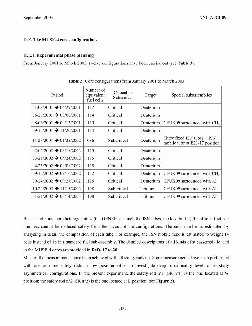
September 2003 ANL-AFCI-092
-16-
II.E. The MUSE-4 core configurations
II.E.1. Experimental phase planning
From January 2001 to March 2003, twelve configurations have been carried out (see Table 3).
Table 3: Core configurations from January 2001 to March 2003
Period Number of equivalent fuel cells
Critical or Subcritical Target Special subassemblies
01/08/2001 06/29/2001 1112 Critical Deuterium
06/29/2001 08/06/2001 1114 Critical Deuterium
08/06/2001 09/13/2001 1119 Critical Deuterium CFUK09 surrounded with CH2
09/13/2001 11/20/2001 1114 Critical Deuterium
11/23/2001 01/25/2002 1086 Subcritical Deuterium Three fixed ISN tubes + ISN mobile tube at E23-17 position
02/06/2002 03/18/2002 1115 Critical Deuterium
03/21/2002 04/24/2002 1115 Critical Deuterium
04/25/2002 09/08/2002 1115 Critical Deuterium
09/12/2002 09/16/2002 1132 Critical Deuterium CFUK09 surrounded with CH2
09/24/2002 09/27/2002 1125 Critical Deuterium CFUK09 surrounded with Al
10/22/2002 11/15/2002 1108 Subcritical Tritium CFUK09 surrounded with Al
01/21/2002 03/14/2003 1108 Subcritical Tritium CFUK09 surrounded with Al
Because of some core heterogeneities (the GENEPI channel, the ISN tubes, the lead buffer) the official fuel cell
numbers cannot be deduced safely from the layout of the configurations. The cells number is estimated by
analysing in detail the composition of each tube. For example, the ISN mobile tube is estimated to weight 14
cells instead of 16 in a standard fuel sub-assembly. The detailed descriptions of all kinds of subassembly loaded
in the MUSE-4 cores are provided in Refs. 17 to 20.
Most of the measurements have been achieved with all safety rods up. Some measurements have been performed
with one or more safety rods in low position either to investigate deep subcriticality level, or to study
asymmetrical configurations. In the present experiment, the safety rod n°1 (SR n°1) is the one located at W
position; the safety rod n°2 (SR n°2) is the one located at E position (see Figure 2).

September 2003 ANL-AFCI-092
-17-
Figure 2: Position of the safety rods n°1 and 2 in the core.
II.E.2. Main measurements performed on the various configurations
From October 2000 to March 2003, twelve configurations have been investigated. Each of them is characterised
by an equivalent fuel cells number. These configurations were as follows:
• 01/08/2001 06/29/2001: critical configuration with 1112 fuel cells (see Figure 3, 4, and 5).
This is the first MUSE-4 critical configuration. It was mainly used for safety parameter measurements. This
configuration has also been considered as the reference for the calculations, detailed in Section III, in support to
the MUSE-4 program.
05
06
07
08
091011
12
13
14
15
16
171819
20
21
22
23
24
25
26
27
28
29
30
31
07 08 09 10 11 12 13 14 15 16 17 18 18 17 16 15 14 13 12 11 09 08 07
North
10
South
W
06
ESR n°1
SR n°2
Pilot rod
Safety rod n°2
Safety rod n°1

September 2003 ANL-AFCI-092
-18-
Figure 3: MUSE-4 Critical Reference Configuration – View XY

September 2003 ANL-AFCI-092
-19-
Figure 4: MUSE-4 Reference Configuration – View XZ
Figure 5: MUSE-4 Reference Configuration – View YZ
• 06/29/2001 08/06/2001: critical configuration with 1114 fuel cells (see Figure 6).
Compared to the previous configuration, the only modification consisted of the addition of two fuel cells to
compensate the 241Pu decay. The monitor calibrations were performed during this period.

September 2003 ANL-AFCI-092
-20-
Figure 6: MUSE-4 Reference Configuration 1114 Cells
• 08/06/2001 09/13/2001: critical configuration with 1119 fuel cells (see Figure 7).
Two tubes with high efficiency CFUK09 fission chambers and surrounded with polythene were loaded in the
reflector zone to perform some delayed neutron fraction measurement tests. Five fuel cells were added to
compensate the negative reactivity effect due to the loading of these subassemblies.
05
06
07
08
09
10
11
12
13
14
15
16
17
18
19
20
21
22
23
24
25
26
27
28
29
30
31
07 08 09 10 11 12 13 14 15 16 17 18 18 17 16 15 14 13 12 11 09 08 07
B A
C D
bi1
bi2 bc2
bc1
Radial shielding
Na/SS reflector
E
N
H G
J K
c1 c2
10
S
W
Axial channel in D4
P2A cells
Shielding
Lead channel
Cp
P r
E
Axial channel in E5
bp
Thermocouple
I
L
F
O18-18Radial cut
O18-18Axial cut
poly

September 2003 ANL-AFCI-092
-21-
Figure 7: MUSE-4 Reference Configuration 1119 Cells
• 09/13/2001 11/20/2001: critical configuration with 1114 fuel cells (see Figure 8).
The two special subassemblies used for delayed neutron fraction measurements were unloaded. Then, this period
was mainly dedicated to:
05
06
0708
091011
12
13
14
15
1617
18
19
20
2122
23
24
2526
27
28
29
3031
07 08 09 10 11 12 13 14 15 16 17 18 18 17 16 15 14 13 12 11 09 08 07
B A
C D
bi1
bi2 bc2
bc1
Radial shielding
Na/SS reflector
MUSE-4 reference configuration1119 ZONA2 cells
E
N
H G
J K
c1 c2
10
S
W
Axial channel in D4
P2A cells
Shielding
Lead channel
Cp
P r
E
Axial channel in E5
bp
Thermocouple
I
L
F
O18-18Radial cut
O18-18Axial cut b1 beta effective
tubesb2
poly
CFUK09
CFUK09

September 2003 ANL-AFCI-092
-22-
• the power calibration;
• the importance distribution measurements with a 252Cf source introduced in East/West and North/South
radial channels and four axial channels (E19-18, W22-17, E16-15, W20-18);
• the irradiation of thick foils of various isotopes within the frame of the CEA/PSI collaboration [14].
Figure 8: MUSE-4 Reference Configuration 1114 Cells
05
06
0708
091011
12
13
1415
16
17
18
19
20
2122
23
24
25
26
27
2829
30
31
07 08 09 10 11 12 13 14 15 16 17 18 18 17 16 15 14 13 12 11 09 08 07
B A
C D
bi1
bi2 bc2
bc1
Radial shielding
Na/SS reflector
E
N
H G
J K
c1 c2
10
S
W
Axial channel in D4
P2A cells
Shielding
Lead channel
Cp
P r
E
Axial channel in E5
bp
Thermocouple
I
L
F
O18-18Radial cut
O18-18Axial cut
poly

September 2003 ANL-AFCI-092
-23-
On November 13, 2001, the safety authorization to perform the experimental program with subcritical
configurations was obtained. The subassemblies loading/unloading operations to move from the reference
critical configuration to the SC0 subcritical configuration began on 11/20/2001 and ended on 11/23/2001 .
• 11/23/2001 01/25/2002 : subcritical configuration with 1086 fuel cells (see Figure 9).
The first coupling of GENEPI and MASURCA with all rods up occurred on November 27, 2001. The reactivity
level was about –167 cents. In December, the annual statutory tests were performed. Then, a short measurement
program was performed in January 2002 to test and to improve the CEA acquisition system performances. This
configuration included the three fixed ISN subassemblies as well as the ISN mobile tube at the E23-17 position.
Figure 9: MUSE-4 SC0 Configuration 1086 Cells
0506
0708
091011
12
1314
15
1617
18
1920
2122
23
2425
26
2728
29
3031
07 08 09 10 11 12 13 14 15 16 17 18 18 17 16 15 14 13 12 11 09 08 07
B A
C D
bi1
bi2 bc2
bc1
shieldingRadial
reflectorNa/SS
E
North
H G
J K
10
South
W
Axial channel in D4 position
E
Axial channel in E5 position
bp
I
L
F
Fuel
Tubes ISN FixesTube ISN Mobile en position 1
3
2
1
1

September 2003 ANL-AFCI-092
-24-
• 02/06/2002 03/18/2002: critical configuration with 1115 fuel cells (see Figure 10).
After a short measurement program in a clean sub critical state (clean means "with all control rods up"), the
reference configuration was carried out again. One more fuel cell was loaded to compensate the 241Pu decay.
Noise techniques were performed with the pilot rod down. The corresponding reactivity level of this
configuration was determined by the well known modified source method (MSM) using the twelve detectors
located in the core and radial reflector: ρ = -0,352 ± 0,02 $ (1$=1βeff). Nevertheless, the MSM factors used to
infer this reference reactivity level were calculated considering a critical configuration with 1112 fuel cells [21].
Figure 10: MUSE-4 Reference Configuration 1115 Cells
05
06
07
08
091011
12
13
14
15
16
17
18
19
20
21
22
23
24
25
26
27
28
29
30
31
07 08 09 10 11 12 13 14 15 16 17 18 18 17 16 15 14 13 12 11 09 08 07
B A
C D
bi1
bi2 bc2
bc1
Radial shielding
Na/SS reflector
E
N
H G
J K
c1 c2
10
S
W
Axial channel in D4Shielding
Lead channel
Cp
P r
E
Axial channel in E5
bp
Thermocouple
I
L
F
O18-18 Radial cut
O18-18Axial cut
12
P2A cells
3
poly

September 2003 ANL-AFCI-092
-25-
• 03/21/2002 04/24/2002: critical configuration with 1115 fuel cells (see Figure 11).
Monitors A and B were respectively reversed with G and H. The first phase of time marking measurements
continued in this configuration. Sub critical configurations were obtained by inserting the pilot rod or a safety
rod.
Figure 11: MUSE-4 Reference Configuration 1115 Cells
• 04/25/2002 09/08/2002 : critical configuration with 1115 fuel cells (see Figure 12).
05
06
07
08091011
12
1314
15
16
17
18
1920
2122
23
24
25
26
27
28
2930
31
07 08 09 10 11 12 13 14 15 16 17 18 18 17 16 15 14 13 12 11 09 08 07
H G
C D
bi1
bi2 bc2
bc1
Radial shielding
Na/SS reflector
East
North
B A
J K
c1 c2
10
South
West
Cp
P r
E
bp
I
L
F
12
3
Apoly
axial channel in D4shielding
lead
axial channel in E5
thermocouple P2A cells
Fuel

September 2003 ANL-AFCI-092
-26-
The monitors A and B were again reversed with G and H. At delayed critical (~-330 pcm), an extensive
measurement program was carried out. Reaction rate traverses and spectral indices were performed for fourteen
isotopes: 10B, 237Np, 233U, 235U, 238U, 238Pu, 239Pu, 240Pu, 241Pu, 242Pu, 241Am, 243Am, 244Cm (only indices) and 232Th. These acquisitions were carried out in six different channels (two radial and four axial). The entire list of
all the reaction rates and spectral indices performed on this configuration is presented in Ref. 14. One will note
that:
• some measurements with 10B chamber are unusable. The operating conditions for this detector are too
complicated. Moreover, this kind of detector is not really suitable for fast spectra.
• The 241Pu fission chamber is rather old and it contains an important amount of Am241.
Figure 12: MUSE-4 Reference Configuration 1115 Cells
0506
07
08091011
1213
1415
16
1718
1920
2122
23
2425
2627
2829
3031
07 08 09 10 11 12 13 14 15 16 17 18 18 17 16 15 14 13 12 11 09 08 07
B A
C D
bi1
bi2 bc2
bc1
Radial shielding
Na/SS reflector
E
N
H G
J K
c1 c2
10
S
W
Axial channel in D4Shielding
Lead channel
Cp
P r
E
Axial channel in E5
bp
thermocouple
I
L
F
O18-18Radial cut
O18-18Axial cut
12
P2A cells
3
poly

September 2003 ANL-AFCI-092
-27-
Several sub critical states were also carried out, with safety rod n°2 and/or the pilot rod inserted, to perform
noise measurements.
Two foil irradiations were performed at the same time within the frame of the CEA/PSI collaboration.
• 09/12/2002 09/16/2002: critical configuration with 1132 fuel cells (see Figure 13).
Two special subassemblies with a high efficiency 235U fission chamber (CFUK09) inside, were loaded to
perform βeff measurements in current mode. The fission chamber was surrounded with CH2 to increase the signal
and the correlation level. During this period, the connection between CFUK09 and the acquisition system had to
be set up under the core. The safety policy authorized this temporary solution until the end of March 2003. This
modification needs no safety requirement.
Figure 13: MUSE-4 Reference Configuration 1132 Cells
05
06
07
08
091011
12
13
14
15
16
17
18
19
20
21
22
23
24
25
26
27
28
29
30
31
07 08 09 10 11 12 13 14 15 16 17 18 18 17 16 15 14 13 12 11 09 08 07
M G
H N
bi1
bi2 bc2
bc1
ECRANRADIAL
COUVERTURENa/SS
East
North
B A
J K
10
South
West
axial channel in D4 position
E
axial channel in E5 position
bp
I
L
F
Fuel
CFUK09
CFUK09
Zone à charger

September 2003 ANL-AFCI-092
-28-
• 09/24/2002 09/27/2002: critical configuration with 1125 fuel cells (see Figure 14).
The two previous special subassemblies used for βeff measurements were unloaded to replace CH2 by aluminum
around the fission chamber. In such conditions, there is not enough correlation and it was shown that it was not
possible to have satisfying βeff values.
Figure 14: MUSE-4 Reference Configuration 1125 Cells
• 10/22/2002 11/15/2002: SC0 subcritical configuration with the (t,d) target (see Figure 15).
05
06
07
08
091011
12
13
14
15
16
17
18
19
20
21
22
23
24
25
26
27
28
29
30
31
07 08 09 10 11 12 13 14 15 16 17 18 18 17 16 15 14 13 12 11 09 08 07
M G
H N
bi1
bi2 bc2
bc1
shieldingRadial
reflectorNa/SS
East
North
A B
J K
10
South
West
axial channel in D4
E
axial channel in E5
bp
I
L
F
Fuel
CFUK09
CFUK09
shielding
lead channel
P2A cells
05
06
07
08
091011
12
13
14
15
16
17
18
19
20
21
22
23
24
25
26
27
28
29
30
31
07 08 09 10 11 12 13 14 15 16 17 18 18 17 16 15 14 13 12 11 09 08 07
M G
H N
bi1
bi2 bc2
bc1
shieldingRadial
reflectorNa/SS
East
North
A B
J K
10
South
West
axial channel in D4 position
E
axial channel in E5 position
bp
I
L
F
Fuel
CFUK09
CFUK09

September 2003 ANL-AFCI-092
-29-
This configuration showed the real beginning of measurement campaigns with clean sub critical configurations
("clean" means "with all rods up"). The number of fuel cells was reduced to 1108, which corresponds to a
subcriticality level of –190 cents. The ISN mobile tube was not loaded. 235U reaction rate traverses and spectral indices were performed in the 2 radial experimental channels with
GENEPI ON.
Figure 15: MUSE-4 SC0 Configuration 1108 Cells
05
0607
08091011
12
1314
1516
1718
19
2021
2223
24
2526
2728
2930
31
07 08 09 10 11 12 13 14 15 16 17 18 18 17 16 15 14 13 12 11 09 08 07
M G
H N
bi1
bi2 bc2
bc1
ECRANRADIAL
COUVERTURENa/SS
East
North
B A
J K
10
South
West
axial channel in D4 position
E
axial channel in E5 position
bp
I
L
F
Fuel
CFUK09
CFUK09
Tubes ISN

September 2003 ANL-AFCI-092
-30-
• 11/15/2002 01/20/2003: no measurement
The (t,d) target was replaced by the (t,t) target from November 18 th to November 22 th. Then, annual statutory
tests have been carried out until the end of the year 2002. During this period, some work on GENEPI was
achieved. In particular, the GENEPI filament was changed three times. Several electronic components were also
replaced.
These modifications were not foreseen and generated a delay of two weeks.
• 01/21/2002 03/14/2003: SC0 subcritical configuration with the (t,t) target (see Figure 16).
The source calibration was from January 21st to January 24th.
Then, 235U and 238U reaction rate traverses and spectral indices were performed in the 2 radial experimental
channels with GENEPI ON. 235U reaction rates traverse and spectrum indices were also performed in the NS
radial experimental channel with GENEPI OFF.
Adjoint flux importance distributions and jerk measurements with a 252Cf source introduced in the East/West
radial channel were performed. This external source was about 2.05 109 n/s on November 11, 2002. In
collaboration with PSI, irradiations of thick foils of various isotopes were performed.
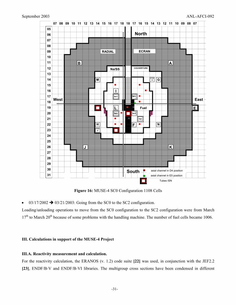
September 2003 ANL-AFCI-092
-31-
Figure 16: MUSE-4 SC0 Configuration 1108 Cells • 03/17/2002 03/21/2003: Going from the SC0 to the SC2 configuration.
Loading/unloading operations to move from the SC0 configuration to the SC2 configuration were from March
17th to March 20th because of some problems with the handling machine. The number of fuel cells became 1006.
III. Calculations in support of the MUSE-4 Project
III.A. Reactivity measurement and calculation.
For the reactivity calculation, the ERANOS (v. 1.2) code suite [22] was used, in conjunction with the JEF2.2
[23], ENDF/B-V and ENDF/B-VI libraries. The multigroup cross sections have been condensed in different
05
06
07
08
091011
12
13
1415
16
17
18
19
2021
22
23
24
2526
27
28
29
30
31
07 08 09 10 11 12 13 14 15 16 17 18 18 17 16 15 14 13 12 11 09 08 07
M G
H N
bi1
bi2 bc2
bc1
ECRANRADIAL
COUVERTURENa/SS
East
North
B A
J K
10
South
West
axial channel in D4 position
E
axial channel in E5 position
bp
I
L
F
Fuel
CFUK09
CFUK09
Tubes ISN
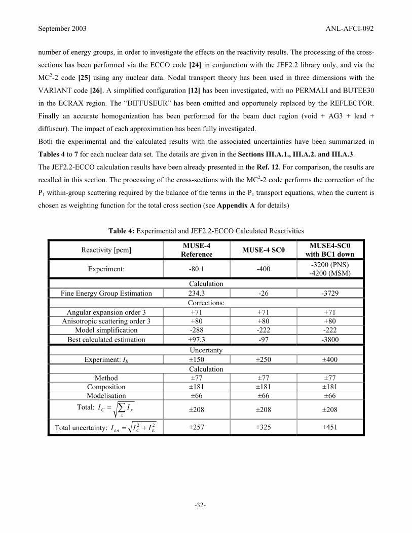
September 2003 ANL-AFCI-092
-32-
number of energy groups, in order to investigate the effects on the reactivity results. The processing of the cross-
sections has been performed via the ECCO code [24] in conjunction with the JEF2.2 library only, and via the
MC2-2 code [25] using any nuclear data. Nodal transport theory has been used in three dimensions with the
VARIANT code [26]. A simplified configuration [12] has been investigated, with no PERMALI and BUTEE30
in the ECRAX region. The “DIFFUSEUR” has been omitted and opportunely replaced by the REFLECTOR.
Finally an accurate homogenization has been performed for the beam duct region (void + AG3 + lead +
diffuseur). The impact of each approximation has been fully investigated.
Both the experimental and the calculated results with the associated uncertainties have been summarized in
Tables 4 to 7 for each nuclear data set. The details are given in the Sections III.A.1., III.A.2. and III.A.3.
The JEF2.2-ECCO calculation results have been already presented in the Ref. 12. For comparison, the results are
recalled in this section. The processing of the cross-sections with the MC2-2 code performs the correction of the
P1 within-group scattering required by the balance of the terms in the P1 transport equations, when the current is
chosen as weighting function for the total cross section (see Appendix A for details)
Table 4: Experimental and JEF2.2-ECCO Calculated Reactivities
Reactivity [pcm] MUSE-4 Reference MUSE-4 SC0 MUSE4-SC0
with BC1 down
Experiment: -80.1 -400 -3200 (PNS) -4200 (MSM)
Calculation Fine Energy Group Estimation 234.3 -26 -3729
Corrections: Angular expansion order 3 +71 +71 +71
Anisotropic scattering order 3 +80 +80 +80 Model simplification -288 -222 -222
Best calculated estimation +97.3 -97 -3800 Uncertanty
Experiment: IE ±150 ±250 ±400 Calculation
Method ±77 ±77 ±77 Composition ±181 ±181 ±181 Modelisation ±66 ±66 ±66
Total: ∑=x
xC II ±208 ±208 ±208
Total uncertainty: 22ECtot III += ±257 ±325 ±451

September 2003 ANL-AFCI-092
-33-
Table 5: Experimental and ENDF/B-V-MC2-2 Calculated Reactivities
Reactivity [pcm]: MUSE-4 Reference MUSE-4 SC0 MUSE4-SC0
with BC1 down
Experiment -80.1 -400 -3200 (PNS) -4200 (MSM)
Calculation Fine Energy Group Estimation 177.7 -94.6 -3781
Corrections: Angular expansion order 3 +43 +43 +43
Anisotropic scattering order 3 +111 +111 +111 Model simplification -288 -222 -222
Best calculated estimation 47.7 -158.6 -3845 Uncertanty
Experiment: IE ±150 ±250 ±400 Calculation
Method ±77 ±77 ±77 Composition ±181 ±181 ±181 Modelisation ±66 ±66 ±66
Total: ∑=x
xC II ±208 ±208 ±208
Total uncertainty: 22ECtot III += ±257 ±325 ±451
Table 6: Experimental and ENDF/B-VI- MC2-2 Calculated Reactivities
Reactivity [pcm]: MUSE-4 Reference MUSE-4 SC0 MUSE4-SC0
with BC1 down
Experiment -80.1 -400 -3200 (PNS) -4200 (MSM)
Calculation Fine Energy Group Estimation 826.0 527.6 -3012
Corrections: Angular expansion order 3 +47 +47 +47
Anisotropic scattering order 3 +116 +116 +116 Model simplification -288 -222 -222
Best calculated estimation 711 478.6 -3061 Uncertainty
Experiment: IE ±150 ±250 ±400 Calculation
Method ±77 ±77 ±77 Composition ±181 ±181 ±181 Modelisation ±66 ±66 ±66
Total: ∑=x
xC II ±208 ±208 ±208
Total uncertainty: 22ECtot III += ±257 ±325 ±451

September 2003 ANL-AFCI-092
-34-
Table 7: Experimental and JEF2.2- MC2-2 Calculated Reactivities
Reactivity [pcm]: MUSE-4 Reference MUSE-4 SC0 MUSE4-SC0
with BC1 down
Experiment -80.1 -400 -3200 (PNS) -4200 (MSM)
Calculation Fine Energy Group Estimation 362.5 207.3 -3415
Corrections: Angular expansion order 3 +57 +57 +57
Anisotropic scattering order 3 +82 +82 +82 Model simplification -288 -222 -222
Best calculated estimation 199.5 110.3 -3512 Uncertanty
Experiment: IE ±150 ±250 ±400 Calculation
Method ±77 ±77 ±77 Composition ±181 ±181 ±181 Modelisation ±66 ±66 ±66
Total: ∑=x
xC II ±208 ±208 ±208
Total uncertainty: 22ECtot III += ±257 ±325 ±451
III.A.1. MUSE-4 reference configuration
For the MUSE-4 reference critical configuration (see Figure 3) the reactivity scale has been determined by the
usual techniques employed on the MASURCA facility and consequently the measured reactivity level of the
experimental loading, with the Pilot rod (PR rod) fully inserted [17] is:
Keff = 0.99920 ± 0.00150; (ρ = -80.1 ± 150 pcm).
The determination of the reactivity level has been achieved through different steps as follows.
1. Effect due to the energy group number.
The simplifications performed on the model allowed to use a double symmetry with respect to the axes X
and Z. In this condition a deterministic calculation with an higher number of energy groups (NG) compared
with the usual 33 groups simulations was possible (NG=838 in the JEF2-ECCO case, NG=887 when
processing the cross-sections with the MC2-2 code). The following table shows the reactivity change with
NG and Figures 17 to 20 show the results of an extrapolation up to the fine group structure (NG=1968 and
NG=2032 in the ECCO and MC2-2 case respectively).

September 2003 ANL-AFCI-092
-35-
Table 8: MUSE-4 Reference Configuration - Keff ECCO - VARIANT JEF2.2 - ECCO
NG VARIANT(1) - ERANOS: Keff ρ [pcm]
33 (2) 0.989920 -1018.3 299 (2) 0.999191 -81.0 471 (2) 1.000556 55.6 838 (2) 1.001788 178.5
Table 9: MUSE-4 Reference Configuration - Keff MC2-2 - VARIANT ENDF/B-V – MC2-2 ENDF/B-VI – MC2-2 JEF2.2 – MC2-2
NG VARIANT(1) - ERANOS: Keff ρ [pcm]
VARIANT(1) - ERANOS: Keff ρ [pcm]
VARIANT(1) - ERANOS: Keff ρ [pcm]
33 (2) 0.986766 -1341.2 0.993063 -698.5 0.990570 -952 231 (2) 0.994357 -567.5 0.999737 -26.3 0.996389 -362.4 460 (2) 0.998390 -161.3 1.004710 468.8 0.999894 -10.6 887 (2) 1.000866 86.5 1.007437 738.2 1.002668 266.1
(1) Flux and leakage expansion order 3 WITH SIMPLIFIED SPHERICAL HARMONIC (HS) (2) With condensation from a fine step to NG
-1200
-1000
-800
-600
-400
-200
0
200
400
0 200 400 600 800 1000 1200 1400 1600 1800 2000NG
Rea
ctiv
ity [p
cm]
CalculatedEstimated
55.8 pcm
Figure 17: MUSE-4 Ref. - Reactivity JEF2.2 – ECCO
-1400
-1200
-1000
-800
-600
-400
-200
0
200
400
0 200 400 600 800 1000 1200 1400 1600 1800 2000NG
Reac
tivity
[pcm
]
CalculatedEstimated
91.2 pcm
Figure 18: MUSE-4 Ref. - Reactivity ENDF/B-V – MC2-2
-800
-600
-400
-200
0
200
400
600
800
1000
0 200 400 600 800 1000 1200 1400 1600 1800 2000NG
Reac
tivity
[pcm
]
CalculatedEstimated
87.8 pcm
Figure 19: MUSE-4 Ref. - Reactivity ENDF/B-VI – MC2-2
-1000
-800
-600
-400
-200
0
200
400
0 200 400 600 800 1000 1200 1400 1600 1800 2000NG
Reac
tivity
[pcm
]
CalculatedEstimated
96.4 pcm
Figure 20: MUSE-4 Ref. - Reactivity JEF2.2 – MC2-2

September 2003 ANL-AFCI-092
-36-
The multiplication factor (reactivity) at the end of the step 1 is:
JEF2.2-ECCO-VARIANT: Keff = 1.002349 (ρ = 234.3 pcm)
ENDF/B-V – MC2-2 – VARIANT: Keff = 1.001780 (ρ = +177.7 pcm)
ENDF/B-VI – MC2-2 – VARIANT: Keff = 1.008329 (ρ = +826.0 pcm)
JEF2.2 – MC2-2 – VARIANT: Keff = 1.003638 (ρ = +362.5 pcm)
2. Effect due to the flux and leakage full angular expansion order 3 (P3) in the transport calculation.
The order of this correction has been taken from the Benchmark calculation, where it was calculated with
NG=33 for the MUSE3 REF configuration [12]:
Table 10: MUSE4 Critical Config. - Transport P3 (Full Flux and Leakage Expansion Order 3) Correction MUSE4 Critical – NG=33 HS – ρ [pcm] P3 – ρ [pcm] ∆ ρ = P3 - HS
JEF2.2 – ECCO -1354 -1283 +71 ENDF/B-V – MC2-2 1530 1577 +47 ENDF/B-VI – MC2-2 2292 2349 +57
JEF2.2 – MC2-2 2304 2347 +43
The multiplication factor (reactivity) at the end of the step 2 is:
JEF2.2-ECCO-VARIANT: Keff = 1.003062 (ρ = 305.3 pcm)
ENDF/B-V – MC2-2 – VARIANT: Keff = 1.002252 (ρ = 224.7 pcm)
ENDF/B-VI – MC2-2 – VARIANT: Keff = 1.008909 (ρ = 883.0 pcm)
JEF2.2 – MC2-2 – VARIANT: Keff = 1.004072 (ρ = 405.5 pcm)
3. Effect due to the anisotropic order 3 (P3) transport calculation.
The order of this correction has been taken from the Benchmark calculation, where it was calculated with
NG=33 for the MUSE3 REF configuration [12]:
Table 11: MUSE4 Critical Configuration - Anisotropic Order 3 Transport Correction MUSE4 Critical – NG=33 P1 – ρ [pcm] P3 – ρ [pcm] ∆ρ = P3 – P1
JEF2.2 – ECCO -1354 -1274 +80 ENDF/B-V – MC2-2 1530 1641 +111 ENDF/B-VI – MC2-2 2292 2408 +116
JEF2.2 – MC2-2 2304 2386 +82
The multiplication factor (reactivity) at the end of the step 3 is:
JEF2.2-ECCO-VARIANT: Keff = 1.003868 (ρ = 385.3 pcm)
ENDF/B-V – MC2-2 – VARIANT: Keff = 1.003368 (ρ = 335.7 pcm)

September 2003 ANL-AFCI-092
-37-
ENDF/B-VI – MC2-2 – VARIANT: Keff = 1.010091 (ρ = 999.0 pcm)
JEF2.2 – MC2-2 – VARIANT: Keff = 1.004899 (ρ = 487.5 pcm)
4. Effect due to the geometrical simplification of the model.
The order of this impact is essentially due to the omission of the structures PERMALI, BUTEE and
“DIFFUSEUR”, of the measurement channels and to the homogenization of the beam duct. The effects have
been separately investigated and even if they have been calculated via JEF2.2-ECCO they are supposed to
be the same for each simulation.
– Omission of PERMALI. The correction has been evaluated with a 3D transport calculation and 33
energy groups, anisotropic scattering order 1 (P1), simplified spherical harmonics (HS): ∆ρ (with –
without PERMALI) = -1 pcm
– Omission of BUTEE. The correction has been evaluated with a 3D transport calculation and 33 energy
groups, anisotropic scattering order 1 (P1), simplified spherical harmonics (HS): ∆ρ (with – without
BUTEE) = -11 pcm
– Omission of the “DIFFUSEUR”. The correction has been evaluated for a RZ model representing the
MUSE3 configuration with a S8P1 transport calculation and 33 energy groups: ∆ρ (with – without
“DIFFUSEUR”) = -296 pcm.
The result has been validated by a Monte-Carlo calculation.
– Omission of the measurement channel. The correction hasn’t been provided yet by the experimentalists
for the MUSE-4 configurations. It has been taken from the previous experiment MUSE3: ∆ρ (with –
without measurement channels) = -66 pcm.
– Homogenization of the beam duct. The correction has been estimated comparing the results obtained
with the homogenized composition and with a more accurate description of the beam duct (AG3 and
void region separated). The calculations have been performed in transport 3D with 33 energy groups,
anisotropic scattering order 1 (P1), simplified spherical harmonics (HS): ∆ρ (homogenized – no
homogenized beam duct) = +86 pcm.
The total effect from the geometrical simplifications of the model is -288 pcm.
The multiplication factor (reactivity) at the end of the step 3 is:
JEF2.2-ECCO-VARIANT: Keff = 1.000974 (ρ = 97.3 pcm)
ENDF/B-V – MC2-2 – VARIANT: Keff = 1.000477 (ρ = 47.7 pcm)
ENDF/B-VI – MC2-2 – VARIANT: Keff = 1.007161 (ρ = 711.0 pcm)
JEF2.2 – MC2-2 – VARIANT: Keff = 1.001999 (ρ = 199.5 pcm)

September 2003 ANL-AFCI-092
-38-
5. Effect due to the Pu241 decay.
This effect is supposed null for the present analysis as the compositions have been updated to the date of the
experiment: January 9, 2001.
Taking in account all the correction above mentioned, the best estimated result for the calculated multiplication
factor consequently is:
JEF2.2-ECCO-VARIANT: Keff = 1.000974 (ρ = 97.3 pcm)
ENDF/B-V – MC2-2 – VARIANT: Keff = 1.000477 (ρ = 47.7 pcm)
ENDF/B-VI – MC2-2 – VARIANT: Keff = 1.007161 (ρ = 711.0 pcm)
JEF2.2 – MC2-2 – VARIANT: Keff = 1.001999 (ρ = 199.5 pcm)
In order to compare the calculation with the experiment, one should take into account the uncertainty associated
both with the simulation and the experiment. In this context, for the MUSE-4 reference configuration the
uncertainty associated to the reactivity measurement has been estimated to be equal to IE = 150 pcm. Concerning
the calculation, the uncertainty has been determined as follows:
1. Uncertainty associated to the calculation method.
The same value adopted for the MUSE3 analysis has been applied. It was determined with a comparison of
the Keff values obtained with TRIPOLI-4 (KT4, with its associated dispersion IT4) and an optimized
deterministic JEF2.2-ECCO-ERANOS calculation (KER with its associated dispersion IER = | KER - KT4|). The
total uncertainty 24T
2ERmeth III += of 77 pcm was estimated. The same uncertainty is assumed to apply to
each simulation.
2. Uncertainty associated to the compositions.
The value has been taken from previous studies, where it was deduced from the accuracy associated to the
chemical analysis of the components of each medium: Icompo = 181 pcm (1σ). The same uncertainty is
supposed to apply to each simulation.
3. Uncertainty associated to the modelization.
As in the previous experiment MUSE3, a constant uncertainty of 20% (1σ) of each correction (omission of
BUTEE, PERMALI, DIFFUSEUR, measurement channels and homogenization of the beam duct) has been
applied. Finally, an uncertainty Itemp = 15 pcm is associated to the reproducibility of the experiment and
another one, Iload = 13 pcm, refers to the loading of the core (indeed we don’t take in account the exact
loading, but an average lot of rodlets). The total uncertainty obtained by the square root of the sum of the
square of each component is Imod = 66 pcm. The same uncertainty is supposed to apply to each simulation.

September 2003 ANL-AFCI-092
-39-
With the assumption that the different sources of uncertainty are completely non-correlated, the total uncertainty
associated to the calculated reactivity value is Icalc = 208 pcm.
Finally, the total absolute uncertainty: 2calc
2Etot III += = 257 pcm.
The following observations can be made:
• This study shows a strong dependence of the calculated reactivity value on the number of energy groups
used. Indeed, in order to accurately account for the spectral effects at the interface core/reflector a detailed
multigroup energy treatment is needed [27]. By the way, significant difficulties occur when performing a
deterministic calculation with a high number of energy groups: the computational resources, in term of time,
disk space and memory, are very demanding. For this purpose, in Appendix B we propose different methods
to process correctly the cross-sections over a broad group energy structure (e.g. with the usual NG=33), able
to reproduce the same results (reactivity and reaction rate distributions) of the fine spatial calculation;
• The impact on the reactivity calculation due to the use of different nuclear data can be observed when the
cross-sections are processed with the MC2-2 code: moving from the ENDF/B-V to the ENDF/B-VI library
causes a spread on the reactivity results of about 700 pcm. While the comparison between the JEF2.2-ECCO
and JEF2.2- MC2-2 results allows to estimate the effect due to the use of different codes (ECCO vs MC2-2)
when the nuclear data are the same: this effect is of about 150 pcm for the present configuration;
• The experiment-calculation discrepancy observed on the reactivity values fit well within the margin of the
uncertainty in the cases JEF2.2-ECCO and ENDF/B-V - MC2-2 (∆ ρ = 177 and 17 pcm respectively). Some
difficulties appear when using the MC2-2 code in conjunction with the JEF2.2 and ENDF/B-VI data. Note
that among the sources of uncertainties there is of course also the uncertainty associated to the nuclear data
that has not been considered in the present analysis.
III.A.2. MUSE-4 SC0 reference configuration
In this section the MUSE-4 SC0 configuration with pilot rod (PR) up has been investigated (see Figure 9).
The measured reactivity is -400 ± 250 pcm.
For reactivity calculations, the same procedure as for the reference configuration has been used.
The following table shows the reactivity change through NG and Figures 21 to 24 show the results of an
extrapolation up to the fine group structure (NG=1968 and NG=2032 in the ECCO and MC2-2 case
respectively). Note that the experimental channels are already included in the simulation.

September 2003 ANL-AFCI-092
-40-
Table 12: MUSE-4 SC0 Configuration with BP Out - Keff ECCO - VARIANT JEF2.2 - ECCO
NG VARIANT(1) - ERANOS: Keff ρ [pcm]
33 (2) 0.987321 -1284.2 299 (2) 0.996572 -344 471 (2) 0.997990 -201.4 838 (2) 0.999234 -76.7
Table 13: MUSE-4 SC0 Configuration with BP Out - Keff MC2-2 - VARIANT ENDF/B-V – MC2-2 ENDF/B-VI – MC2-2 JEF2.2 – MC2-2
NG VARIANT(1) - ERANOS: Keff ρ [pcm]
VARIANT(1) - ERANOS: Keff ρ [pcm]
VARIANT(1) - ERANOS: Keff ρ [pcm]
33 (2) 0.984211 -1604.2 0.990405 -968.8 0.989053 -1106.8 231 (2) 0.991704 -836.5 0.996994 -301.5 0.994924 -510.2 460 (2) 0.995727 -429.1 1.001821 181.8 0.998488 -151.4 887 (2) 0.998198 -180.5 1.004589 456.8 1.001204 120.3
(1) Flux and leakage expansion order 3 WITH SIMPLIFIED SPHERICAL HARMONIC (HS) (2) With condensation from a fine step to NG
-1300
-1100
-900
-700
-500
-300
-100
100
0 200 400 600 800 1000 1200 1400 1600 1800 2000NG
Reac
tivity
[pcm
]
CalculatedEstimated
56.7 pcm
Figure 21: MUSE-4 SC0 - Reactivity JEF2.2 – ECCO
-1600
-1400
-1200
-1000
-800
-600
-400
-200
0
0 200 400 600 800 1000 1200 1400 1600 1800 2000
NG
Reac
tivity
[pcm
]
CalculatedEstimated
85.9 pcm
Figure 22: MUSE-4 SC0 - Reactivity ENDF/B-V – MC2-2
-1000
-800
-600
-400
-200
0
200
400
600
0 200 400 600 800 1000 1200 1400 1600 1800 2000NG
Reac
tivity
[pcm
]
CalculatedEstimated
70.8 pcm
Figure 23: MUSE-4 SC0 - Reactivity ENDF/B-VI – MC2-2
-1000
-800
-600
-400
-200
0
200
400
600
0 200 400 600 800 1000 1200 1400 1600 1800 2000NG
Reac
tivity
[pcm
]
CalculatedEstimated
70.8 pcm
Figure 24: MUSE-4 SC0 - Reactivity JEF2.2 – MC2-2

September 2003 ANL-AFCI-092
-41-
After extrapolation to the fine energy group structure, the multiplication factor (reactivity) is:
JEF2.2-ECCO-VARIANT: Keff = 0.999740 (ρ = -26 pcm)
ENDF/B-V – MC2-2 – VARIANT: Keff = 0.999055 (ρ = -94.6 pcm)
ENDF/B-VI – MC2-2 – VARIANT: Keff = 1.005304 (ρ = 527.6 pcm)
JEF2.2 – MC2-2 – VARIANT: Keff = 1.002077 (ρ = 207.3 pcm)
Taking in account all the corrections (angular expansion order 3, anisotropic scattering order 3, geometrical
simplifications of the model) as in the case of the reference configuration and reported in Tables 4 to 7, the best
estimated result for the calculated multiplication factor is:
JEF2.2-ECCO-VARIANT: Keff = 0.999031 (ρ = -97 pcm)
ENDF/B-V – MC2-2 – VARIANT: Keff = 0.998417 (ρ = -158.6 pcm)
ENDF/B-VI – MC2-2 – VARIANT: Keff = 1.004809 (ρ = 478.6 pcm)
JEF2.2 – MC2-2 – VARIANT: Keff = 1.001104 (ρ = 110.3 pcm)
The uncertainty associated to the calculation has been supposed to be the same of the reference configuration.
The uncertainty associated to the experiment is 250 pcm. Consequently the total uncertainty becomes 325.
Investigating the reactivity calculated results and their comparison with the experimental ones, observations
similar to the reference configuration can be made.
The results presented in this section also apply to the MUSE-4 SC0 configuration with pilot rod (PR) inserted if
corrected by the reactivity worth of the pilot rod which has been estimated by the experimentalists equal to -140
pcm.
III.A.3. MUSE-4 SC0 reference configuration with bc1 inserted
In this section the MUSE-4 SC0 configuration with control rod BC1 and pilot rod (PR) inserted has been
investigated (see Figure 9).
The measured reactivity is -3200 pcm (by PNS method), -4200 pcm (by MSM method). The MSM method
determines subcritical reactivities by ratios of count rates corrected for changes in detector efficiencies and
source importance between two subcritical states. In the PNS method, information on the subcritical level is
deduced from the decay of the response P(t) arising from an external neutron pulse.
The wide discrepancy (-4200 vs. –3200 pcm) obtained using the two methods is being investigated by the
experimentalists.
The experimental uncertainty is ± 400 pcm.

September 2003 ANL-AFCI-092
-42-
For reactivity calculations, the same procedure as for the reference configuration has been used.
The following table shows the reactivity change through NG and Figures 25 to 28 show the results of an
extrapolation up to the fine group structure (NG=1968 and NG=2032 in the ECCO and MC2-2 case
respectively). Note that the experimental channels are already included in the simulation.
Table 14: MUSE-4 SC0 Configuration with BC1 and PR Inserted - Keff ECCO - VARIANT JEF2.2 - ECCO
NG VARIANT(1) - ERANOS: Keff ρ [pcm]
33 (2) 0.952524 -4984.2 299 (2) 0.961091 -4048.4 471 (2) 0.962347 -3912.6 838 (2) 0.963489 -3789.5
Table 15: MUSE-4 SC0 Configuration with BC1 and BP Inserted - Keff MC2-2 - VARIANT ENDF/B-V – MC2-2 ENDF/B-VI – MC2-2 JEF2.2 – MC2-2
NG VARIANT(1) - ERANOS: Keff ρ [pcm]
VARIANT(1) - ERANOS: Keff ρ [pcm]
VARIANT(1) - ERANOS: Keff ρ [pcm]
33 (2) 0.949659 -5300.9 0.956657 -4530.7 0.954693 -4745.7 231 (2) 0.956634 -4533.2 0.962812 -3862.4 0.960162 -4149.1 460 (2) 0.960377 -4125.8 0.967314 -3379.1 0.963481 -3790.3 887 (2) 0.962675 -3877.2 0.969900 -3103.4 0.966010 -3518.6
(1) Flux and leakage expansion order 3 WITH SIMPLIFIED SPHERICAL HARMONIC (HS) (2) With condensation from a fine step to NG
-5300
-5100
-4900
-4700
-4500
-4300
-4100
-3900
-3700
-3500
0 200 400 600 800 1000 1200 1400 1600 1800 2000NG
Reac
tivity
[pcm
]
CalculatedEstimated
60.5 pcm
Figure 25: MUSE-4 SC0 (BC1 in) - Reactivity JEF2.2 – ECCO
-5400
-5200
-5000
-4800
-4600
-4400
-4200
-4000
-3800
-3600
0 200 400 600 800 1000 1200 1400 1600 1800 2000NG
Reac
tivity
[pcm
]
CalculatedEstimated
96.2 pcm
Figure 26: MUSE-4 SC0 (BC1 in) - Reactivity ENDF/B-V – MC2-2

September 2003 ANL-AFCI-092
-43-
-4600
-4400
-4200
-4000
-3800
-3600
-3400
-3200
-3000
-2800
0 200 400 600 800 1000 1200 1400 1600 1800 2000NG
Reac
tivity
[pcm
]
CalculatedEstimated
91.4 pcm
Figure 27: MUSE-4 SC0 (BC1 in) - Reactivity ENDF/B-VI – MC2-2
-4800
-4650
-4500
-4350
-4200
-4050
-3900
-3750
-3600
-3450
-3300
0 200 400 600 800 1000 1200 1400 1600 1800 2000NG
Reac
tivity
[pcm
]
CalculatedEstimated
103.6 pcm
Figure 28: MUSE-4 SC0 (BC1 in) - Reactivity JEF2.2 – MC2-2
After extrapolation to the fine energy group structure, the multiplication factor (reactivity) is:
JEF2.2-ECCO-VARIANT: Keff = 0.964051 (ρ = -3729 pcm)
ENDF/B-V – MC2-2 – VARIANT: Keff = 0.963568 (ρ = -3781 pcm)
ENDF/B-VI – MC2-2 – VARIANT: Keff = 0.970761 (ρ = -3012 pcm)
JEF2.2 – MC2-2 – VARIANT: Keff = 0.966978 (ρ = -3415 pcm)
Taking in account all the corrections (angular expansion order 3, anisotropic scattering order 3, geometrical
simplifications of the model) as in the case of the reference configuration and reported in Tables 4 to 7, the best
estimated result for the calculated multiplication factor is:
JEF2.2-ECCO-VARIANT: Keff = 0.963391 (ρ = -3800 pcm)
ENDF/B-V – MC2-2 – VARIANT: Keff = 0.962974 (ρ = -3845 pcm)
ENDF/B-VI – MC2-2 – VARIANT: Keff = 0.970299 (ρ = -3061 pcm)
JEF2.2 – MC2-2 – VARIANT: Keff = 0.966072 (ρ = -3512 pcm)
The uncertainty associated to the calculation has been supposed to be the same of the reference configuration.
The uncertainty associated to the experiment is 400 pcm. Consequently the total uncertainty becomes 451.
Investigating the reactivity calculated results and their comparison with the experimental ones, observations
similar to the reference configuration can be seen. III.B. Adjoint flux measurement and calculation.
We perform in this section the analysis of the experimental traverses with californium source [28] for the
MUSE-4 reference configuration (see Figure 3). These traverses represent the adjoint flux distribution [28].

September 2003 ANL-AFCI-092
-44-
Axial and radial distributions are analyzed. The axial traverses have been performed at the positions E1615,
E1818, W2018 and W2217. The positions E1615 and W2217 are relatively unperturbed, while the position
E1918 is in the lead buffer zone and W2018 is near both to the lead buffer zone and to a control rod. The channel
locations, shown in Figure 3, have also been represented in 3 dimensions in Fig.29 and 30 to provide an
illustration of their configuration:
Figure 29: MUSE-4 Critical Configuration – Horizontal Channels Locations

September 2003 ANL-AFCI-092
-45-
Figure 30: MUSE-4 Critical Configuration – Axial Channels Locations
The traverses were made at two reactivity levels: roughly –70 pcm with the pilot rod (PR) down and roughly –20
pcm with the PR at 600 mm. North-South (NS) and East-West (EW) radial traverses were also performed for the
two reactivities.
The calculation results have been performed with the ERANOS code [22] suite in conjunction with the JEF2.2
[23], ENDF/B-V and ENDF/B-VI libraries. The multigroup cross sections have been condensed in different
number of energy groups, in order to investigate the effects on the calculated adjoint flux traverses. The
processing of the cross-sections has been performed via the ECCO code [24] in conjunction with the JEF2.2
library only, and via the MC2-2 code [25] using any nuclear data. The VARIANT code [26] was used with a
three dimension geometry. All geometrical and material compositions are as shown for the model used to
calculate the reactivity value. Transport theory was used in P1 approximation. The core models assume that the
Reference MUSE-4 configuration contains 1112 fuel cells (as given in Ref. 17). This corresponds to a total fuel
mass of 1550.1 kg (using a mass of 0.697 kg as given in the MASURCA catalogue for MOX in one fuel rod).
Note, however, that due to the Pu241 decay the number of fuel cells to achieve the criticality has increased to

September 2003 ANL-AFCI-092
-46-
1114 in October 2001. It is assumed that the subsequent effect on the calculated traverses is negligible. Then, a
brief discussion on the observed results is given.
The following notation is introduced in the following: “B” as in “E1615B” refers to the deeper subcritical state
(PR down) and “H” as in “E1615H” refers to the case with PR at 600 mm. The normalized adjoint flux has been
measured from the count data according to the following relation:
ro
ri*o
*i
CCCC
ΦΦ
−−
= Eq.1
In this relation, the adjoint flux at the point i relative to the point o is proportional to the counts at those
positions. The value is offset with respect to the reference (point r) by the amount corresponding to the intrinsic
source.
The uncertainties related to the experimental data have been also provided for each monitor channel [28]. It was
assumed that the best estimate of the normalized adjoint flux would be simply the average of the 10 monitor
channels, and the associated uncertainty would be calculated using the following relation:
∑=N
j 2j
2x σ
1σ1 Eq.2
The calculation results show that the model does not accurately fit the adjoint flux outside the core when only 33
energy groups are used. The model consistently underestimates the adjoint flux in all the traverses (see Figures
31 to 55). Indeed, a correct description of the slowing down of the neutrons and their reflection in the fuel at the
interface core/reflector, requires the use of a higher number of energy groups NG [27] (see section III.A).
In fact, the discrepancies are sharply reduced when NG increases. In this case, the calculations performed for
example via JEF2.2-ECCO with NG = 299, 471, 838 show approximately the same results (see e.g. Figure 31),
consequently a 299 energy group structure seems to be enough for the analysis of the experimental data. The
same remark applies when the MC2-2 code is used, but in this case 231 energy groups are employed instead of
299. Using 299 (or 231) energy groups the model still underestimates the adjoint flux, but the observed
discrepancies seem to be within the margins if an uncertainty associated to the calculation would be taken in
account together with the experimental one.
All the measured traverses have been studied, but in the following just the adjoint flux distributions observed
with PR at 600 mm are discussed. Indeed, with PR down the measured and calculated results are about the same;
slight differences appear just in the case of the E1918 traverse which is at the same time close to a control rod
and it is also the closest traverse to the PR.

September 2003 ANL-AFCI-092
-47-
The use of different nuclear data libraries doesn’t seem to affect the calculated adjoint flux distributions if the
same number of energy group is used. In particular, this can be observed in Figures 58 to 61 that compare the
experimental data with the results provided with the ECCO code using the JEF2.2 data and via the MC2-2 code
in conjunction with any library.
However, an asymmetry is observed in some data that is not seen in the model. This is especially true for the
W2018H traverses (see Figures 34, 40, 46, 52 and 58), but it also appears for the E1918H traverse (see Figures
33, 39, 45, 51 and 57). At the present time, it is not clear whether the asymmetries seen in the data correspond to
a real physical effect, or they are due to some bias.
• E1615.
This axial traverse is far from potentially perturbing influences such as the lead buffer and control rods.
Thus, an axial symmetry is expected, and, indeed, a careful examination of the data shows that this is true in
both the cases with PR down and at 600 mm. The same is observed by the calculation.
• E1918.
Even if this traverse passes through the lead buffer that could introduce an axial perturbation, a pretty
symmetric shape, as it is seen in the calculation, would be expected. However, with PR at 600 mm, there is a
shift towards the top of the core, which is not expected. This traverse was made in two steps (negative first,
then positive at a later time), so it is possible that this procedure introduced a bias even though new zero and
reference values were obtained.
• W2018.
This axial traverse, for both PR positions, shows an asymmetry not seen in the calculation. In both cases, the
adjoint flux is higher below the core midplane. The only axial asymmetry that could cause this behavior is
the fact that this traverse is adjacent to a control rod. Normally it would be assumed that when the control
rod is fully inserted there would be a little perturbation, but this is not confirmed by the data. Another
potential cause is the translation of the data due to uncertainty in the position of the device. If the data are
translated 25 mm upwards, we see a much better agreement with the calculation. This translation has been
introduced in Figures 34, 40, 46, 52 and 58.
• W2211.
In this case a complete unperturbed symmetry as for E1615 is expected, and this is confirmed by both data
and calculation.

September 2003 ANL-AFCI-092
-48-
• EW.
In the EW traverse, a slightly higher adjoint flux on the negative (West) side is observed, while the
calculation is completely symmetric. There is an east-west asymmetry because the west side contains
slightly more fuel, and PR is on the East side. More refined calculations are required to investigate this
effect.
• NS.
In the North-South traverse, the data are showing a higher adjoint flux on the negative (north) side, while
the calculation are showing the reverse. It would be expected that the additional lead on the south would
cause an importance enhancement. Because of the anomalous data of W2018, if a 25 mm translation of the
data is performed the agreement with the calculation is improved. This translation has been introduced in
Figures 37, 43, 49, 55 and 61.
In conclusion, there are some traverses that show unexplained anomalies. E1918H is suspicious because of the
fact that the negative traverse was done at a different time than the positive ones, and there is a suspicious 25
mm translation in both the W2018H and NSH traverses. On the contrary, when no perturbation is present from
control rods or lead, as for E1615 and W2217, we see excellent agreement between data and calculations, and
there are no unexplained anomalies.

September 2003 ANL-AFCI-092
-49-
III.B.1. Use of the ECCO code in conjunction with the JEF2.2 data.
0
0.1
0.2
0.3
0.4
0.5
0.6
0.7
0.8
0.9
1
-60 -50 -40 -30 -20 -10 0 10 20 30 40 50 60Z [cm]
Nor
mal
ized
Adj
oint
Flu
x
E1615BE1615H33gr - rho=-1018 pcm299gr - rho=-81pcm471gr - rho=55 pcm838gr - rho=178 pcm
Figure 31: E1615 Effect due to the Energy Groups Number
0
0.1
0.2
0.3
0.4
0.5
0.6
0.7
0.8
0.9
1
-60 -50 -40 -30 -20 -10 0 10 20 30 40 50 60Z [cm]
Norm
aliz
ed A
djoi
nt F
lux
Experiment (E1615H)
33gr - rho=-1018 pcm299gr - rho=-81pcm
Refl. Core Refl.
Figure 32: E1615H: JEF2-ECCO Calc./Exp. Comparison
0
0.1
0.2
0.3
0.4
0.5
0.6
0.7
0.8
0.9
1
1.1
-60 -50 -40 -30 -20 -10 0 10 20 30 40 50 60Z [cm]
Norm
aliz
ed A
djoi
nt F
lux
Experiment (E1918H)
33gr - rho=-1018 pcm
299gr - rho=-81pcm
Refl. Core Lead Core Refl.
Figure 33: E1918H: JEF2-ECCO Calc./Exp. Comparison
0
0.1
0.2
0.3
0.4
0.5
0.6
0.7
0.8
0.9
1
-60 -50 -40 -30 -20 -10 0 10 20 30 40 50 60Z [cm]
Nor
mal
ized
Adj
oint
Flu
x
Experiment (W2018H)33gr - rho=-1018 pcm299gr - rho=-81pcm
Refl. Core Refl.
Figure 34: W2018H: JEF2-ECCO Calc./Exp. Comparison
0
0.1
0.2
0.3
0.4
0.5
0.6
0.7
0.8
0.9
1
-60 -50 -40 -30 -20 -10 0 10 20 30 40 50 60Z [cm]
Nor
mal
ized
Adj
oint
Flu
x
Experiment (W2217H)33gr - rho=-1018 pcm299gr - rho=-81pcm
Refl. Core Refl.
Figure 35: W2217H: JEF2-ECCO Calc./Exp. Comparison

September 2003 ANL-AFCI-092
-50-
0
0.1
0.2
0.3
0.4
0.5
0.6
0.7
0.8
0.9
1
1.1
-75 -60 -45 -30 -15 0 15 30 45 60 75Y [cm]
Nor
mal
ized
Adj
oint
Flu
x
Experiment (EWH)33gr - rho=-1018 pcm299gr - rho=-81pcm
Refl. Core Lead Core Refl.
Figure 36: EWH: JEF2-ECCO Calc./Exp. Comparison
0
0.1
0.2
0.3
0.4
0.5
0.6
0.7
0.8
0.9
1
-75 -65 -55 -45 -35 -25 -15 -5 5 15 25 35 45 55 65 75X [cm]
Nor
mal
ized
Adj
oint
Flu
x
Experiment (NSH)
33gr - rho=-1018 pcm
299gr - rho=-81pcm
Refl. Core Lead Core Refl.
Figure 37: NSH: JEF2-ECCO Calc./Exp. Comparison
III.B.2. Use of the MC2-2 code in conjunction with the ENDF/B-V data.
0
0.1
0.2
0.3
0.4
0.5
0.6
0.7
0.8
0.9
1
-60 -50 -40 -30 -20 -10 0 10 20 30 40 50 60Z [cm]
Nor
mal
ized
Adj
oint
Flu
x
Experiment (E1615H)
33gr - rho=-1341.2 pcm231gr - rho=-567.5 pcm
Refl. Core Refl.
Figure 38: E1615H: ENDF/B-V-MC2-2 Calc./Exp. Comparison
0
0.1
0.2
0.3
0.4
0.5
0.6
0.7
0.8
0.9
1
1.1
-60 -50 -40 -30 -20 -10 0 10 20 30 40 50 60Z [cm]
Nor
mal
ized
Adj
oint
Flu
x
Experiment (E1918H)
33gr - rho=-1341.2 pcm
231gr - rho=-567.5 pcm
Refl. Core Lead Core Refl.
Figure 39: E1918H: ENDF/B-V-MC2-2 Calc./Exp. Comparison
0
0.1
0.2
0.3
0.4
0.5
0.6
0.7
0.8
0.9
1
-60 -50 -40 -30 -20 -10 0 10 20 30 40 50 60Z [cm]
Norm
aliz
ed A
djoi
nt F
lux
Experiment (W2018H)
33gr - rho=-1341.2 pcm
231gr - rho=-567.5 pcm
Refl. Core Refl.
Figure 40: W2018H: ENDF/B-V-MC2-2 Calc./Exp. Comparison
0
0.1
0.2
0.3
0.4
0.5
0.6
0.7
0.8
0.9
1
-60 -50 -40 -30 -20 -10 0 10 20 30 40 50 60Z [cm]
Norm
aliz
ed A
djoi
nt F
lux
Experiment (W2217H)
33gr - rho=-1341.2 pcm
231gr - rho=-567.5 pcm
Refl. Core Refl.
Figure 41: W2217H: ENDF/B-V-MC2-2 Calc./Exp. Comparison

September 2003 ANL-AFCI-092
-51-
0
0.1
0.2
0.3
0.4
0.5
0.6
0.7
0.8
0.9
1
1.1
-75 -60 -45 -30 -15 0 15 30 45 60 75Y [cm]
Nor
mal
ized
Adj
oint
Flu
x
Experiment (EWH)33gr - rho=-1341.2 pcm231gr - rho=-567.5 pcm
Refl. Core Lead Core Refl.
Figure 42: EWH: ENDF/B-V-MC2-2 Calc./Exp. Comparison
0
0.1
0.2
0.3
0.4
0.5
0.6
0.7
0.8
0.9
1
-75 -65 -55 -45 -35 -25 -15 -5 5 15 25 35 45 55 65 75X [cm]
Nor
mal
ized
Adj
oint
Flu
x
Experiment (NSH)33gr - rho=-1341.2 pcm231gr - rho=-567.5 pcm
Refl. Core Lead Core Refl.
Figure 43: NSH: ENDF/B-V-MC2-2 Calc./Exp. Comparison
III.B.3. Use of the MC2-2 code in conjunction with the ENDF/B-VI data.
0
0.1
0.2
0.3
0.4
0.5
0.6
0.7
0.8
0.9
1
-60 -50 -40 -30 -20 -10 0 10 20 30 40 50 60Z [cm]
Nor
mal
ized
Adj
oint
Flu
x
Experiment (E1615H)
33gr - rho=-698.5 pcm231gr - rho=-26.3 pcm
Refl. Core Refl.
Figure 44: E1615H: ENDF/B-VI-MC2-2 Calc./Exp. Comparison
0
0.1
0.2
0.3
0.4
0.5
0.6
0.7
0.8
0.9
1
1.1
-60 -50 -40 -30 -20 -10 0 10 20 30 40 50 60Z [cm]
Nor
mal
ized
Adj
oint
Flu
x
Experiment (E1918H)
33gr - rho=-698.5 pcm
231gr - rho=-26.3 pcm
Refl. Core Lead Core Refl.
Figure 45: E1918H: ENDF/B-VI-MC2-2 Calc./Exp. Comparison
0
0.1
0.2
0.3
0.4
0.5
0.6
0.7
0.8
0.9
1
-60 -50 -40 -30 -20 -10 0 10 20 30 40 50 60Z [cm]
Norm
aliz
ed A
djoi
nt F
lux
Experiment (W2018H)
33gr - rho=-698.5 pcm
231gr - rho=-26.3 pcm
Refl. Core Refl.
Figure 46: W2018H: ENDF/B-VI-MC2-2 Calc./Exp. Comparison
0
0.1
0.2
0.3
0.4
0.5
0.6
0.7
0.8
0.9
1
-60 -50 -40 -30 -20 -10 0 10 20 30 40 50 60Z [cm]
Norm
aliz
ed A
djoi
nt F
lux
Experiment (W2217H)
33gr - rho=-698.5 pcm
231gr - rho=-26.3 pcm
Refl. Core Refl.
Figure 47: W2217H: ENDF/B-VI-MC2-2 Calc./Exp. Comparison

September 2003 ANL-AFCI-092
-52-
0
0.1
0.2
0.3
0.4
0.5
0.6
0.7
0.8
0.9
1
1.1
-75 -60 -45 -30 -15 0 15 30 45 60 75Y [cm]
Nor
mal
ized
Adj
oint
Flu
x
Experiment (EWH)33gr - rho=-698.5 pcm231gr - rho=-26.3 pcm
Refl. Core Lead Core Refl.
Figure 48: EWH: ENDF/B-VI-MC2-2 Calc./Exp. Comparison
0
0.1
0.2
0.3
0.4
0.5
0.6
0.7
0.8
0.9
1
-75 -65 -55 -45 -35 -25 -15 -5 5 15 25 35 45 55 65 75X [cm]
Nor
mal
ized
Adj
oint
Flu
x
Experiment (NSH)33gr - rho=-698.5 pcm231gr - rho=-26.3 pcm
Refl. Core Lead Core Refl.
Figure 49: NSH: ENDF/B-VI-MC2-2 Calc./Exp. Comparison
III.B.4. Use of the MC2-2 code in conjunction with the JEF2.2 data.
0
0.1
0.2
0.3
0.4
0.5
0.6
0.7
0.8
0.9
1
-60 -50 -40 -30 -20 -10 0 10 20 30 40 50 60Z [cm]
Nor
mal
ized
Adj
oint
Flu
x
Experiment (E1615H)
33gr - rho=-952 pcm231gr - rho=-362.4 pcm
Refl. Core Refl.
Figure 50: E1615H: JEF2.2-MC2-2 Calc./Exp. Comparison
0
0.1
0.2
0.3
0.4
0.5
0.6
0.7
0.8
0.9
1
1.1
-60 -50 -40 -30 -20 -10 0 10 20 30 40 50 60Z [cm]
Nor
mal
ized
Adj
oint
Flu
x
Experiment (E1918H)
33gr - rho=-952 pcm
231gr - rho=-362.4 pcm
Refl. Core Lead Core Refl.
Figure 51: E1918H: JEF2.2-MC2-2 Calc./Exp. Comparison
0
0.1
0.2
0.3
0.4
0.5
0.6
0.7
0.8
0.9
1
-60 -50 -40 -30 -20 -10 0 10 20 30 40 50 60Z [cm]
Norm
aliz
ed A
djoi
nt F
lux
Experiment (W2018H)
33gr - rho=-952 pcm
231gr - rho=-362.4 pcm
Refl. Core Refl.
Figure 52: W2018H: JEF2.2-MC2-2 Calc./Exp. Comparison
0
0.1
0.2
0.3
0.4
0.5
0.6
0.7
0.8
0.9
1
-60 -50 -40 -30 -20 -10 0 10 20 30 40 50 60Z [cm]
Norm
aliz
ed A
djoi
nt F
lux
Experiment (W2217H)
33gr - rho=-952 pcm
231gr - rho=-362.4 pcm
Refl. Core Refl.
Figure 53: W2217H: JEF2.2-MC2-2 Calc./Exp. Comparison

September 2003 ANL-AFCI-092
-53-
0
0.1
0.2
0.3
0.4
0.5
0.6
0.7
0.8
0.9
1
1.1
-75 -60 -45 -30 -15 0 15 30 45 60 75Y [cm]
Nor
mal
ized
Adj
oint
Flu
x
Experiment (EWH)33gr - rho=-952 pcm231gr - rho=-362.4 pcm
Refl. Core Lead Core Refl.
Figure 54: EWH: JEF2.2-MC2-2 Calc./Exp. Comparison
0
0.1
0.2
0.3
0.4
0.5
0.6
0.7
0.8
0.9
1
-75 -65 -55 -45 -35 -25 -15 -5 5 15 25 35 45 55 65 75X [cm]
Nor
mal
ized
Adj
oint
Flu
x
Experiment (NSH)33gr - rho=-952 pcm231gr - rho=-362.4 pcm
Refl. Core Lead Core Refl.
Figure 55: NSH: JEF2.2-MC2-2 Calc./Exp. Comparison
III.B.5. Effect due to the nuclear data on the adjoint flux traverses.
0
0.1
0.2
0.3
0.4
0.5
0.6
0.7
0.8
0.9
1
-60 -50 -40 -30 -20 -10 0 10 20 30 40 50 60Z [cm]
Nor
mal
ized
Adj
oint
Flu
x
Experiment (E1615H)299gr JEF2-ECCO (-81 pcm)231gr ENDF/B-V - MC2 (-567.5 pcm)231gr ENDF/B-VI - MC2 (-26.3 pcm)231gr JEF2 - MC2 (-362.4 pcm)
Refl. Core Refl.
Figure 56: E1615H: Nuclear Data Impact on the Calculation
0
0.1
0.2
0.3
0.4
0.5
0.6
0.7
0.8
0.9
1
1.1
-60 -50 -40 -30 -20 -10 0 10 20 30 40 50 60Z [cm]
Nor
mal
ized
Adj
oint
Flu
x
Experiment (E1918H)299gr JEF2-ECCO (-81 pcm)231gr ENDF/B-V - MC2 (-567.5 pcm)231gr ENDF/B-VI - MC2 (-26.3 pcm)231gr JEF2 - MC2 (-362.4 pcm)
Refl. Core Lead Core Refl.
Figure 57: E1918H: Nuclear Data Impact on the Calculation
0
0.1
0.2
0.3
0.4
0.5
0.6
0.7
0.8
0.9
1
-60 -50 -40 -30 -20 -10 0 10 20 30 40 50 60Z [cm]
Norm
aliz
ed A
djoi
nt F
lux
Experiment (W2018H)299gr JEF2-ECCO (-81 pcm)231gr ENDF/B-V - MC2 (-567.5 pcm)231gr ENDF/B-VI - MC2 (-26.3 pcm)231gr JEF2 - MC2 (-362.4 pcm)
Refl. Core Refl.
Figure 58: W2018H: Nuclear Data Impact on the Calculation
0
0.1
0.2
0.3
0.4
0.5
0.6
0.7
0.8
0.9
1
-60 -50 -40 -30 -20 -10 0 10 20 30 40 50 60Z [cm]
Norm
aliz
ed A
djoi
nt F
lux
Experiment (W2217H)299gr JEF2-ECCO (-81 pcm)231gr ENDF/B-V - MC2 (-567.5 pcm)231gr ENDF/B-VI - MC2 (-26.3 pcm)231gr JEF2 - MC2 (-362.4 pcm)
Refl. Core Refl.
Figure 59: W2217H: Nuclear Data Impact on the Calculation

September 2003 ANL-AFCI-092
-54-
0
0.1
0.2
0.3
0.4
0.5
0.6
0.7
0.8
0.9
1
1.1
-75 -60 -45 -30 -15 0 15 30 45 60 75Y [cm]
Nor
mal
ized
Adj
oint
Flu
x
Experiment (EWH)299gr JEF2-ECCO (-81 pcm)231gr ENDF/B-V - MC2 (-567.5 pcm)231gr ENDF/B-VI - MC2 (-26.3 pcm)231gr JEF2 - MC2 (-362.4 pcm)
Refl. Core Lead Core Refl.
Figure 60: EWH: Nuclear Data Impact on the Calculation
0
0.1
0.2
0.3
0.4
0.5
0.6
0.7
0.8
0.9
1
-75 -65 -55 -45 -35 -25 -15 -5 5 15 25 35 45 55 65 75X [cm]
Nor
mal
ized
Adj
oint
Flu
x
Experiment (NSH)299gr JEF2-ECCO (-81 pcm)231gr ENDF/B-V - MC2 (-567.5 pcm)231gr ENDF/B-VI - MC2 (-26.3 pcm)231gr JEF2 - MC2 (-362.4 pcm)
Refl. Core Lead Core Refl.
Figure 61: NSH: Nuclear Data Impact on the Calculation
III.C. Reaction rate traverses measurement and calculation.
U235 fission radial traverses EW and NS, and the Np237 EW radial traverse (see Figures 29 and 30 for the
channel locations) of the MUSE-4 critical configuration (1115 cells) have been calculated. In the following
figures the comparison with the experiment is also performed and the behavior in proximity of the reflector
region has been expanded.
The calculation results have been performed with the ERANOS code [22] suite in conjunction with the JEF2.2
[23], ENDF/B-V and ENDF/B-VI libraries. The multigroup cross sections have been condensed in different
number of energy groups, in order to investigate the effects on the fission rate traverses. The processing of the
cross-sections has been performed via the ECCO code [24] in conjunction with the JEF2.2 library only, and via
the MC2-2 code [25] using any nuclear data. The VARIANT code [26] was used with a three dimension
geometry. All geometrical and material compositions are as shown for the model used to calculate the reactivity
value. Transport theory was used in P1 approximation. The core models assume that the Reference MUSE-4
configuration contains 1112 fuel cells. This corresponds to a total fuel mass of 1550.1 kg (using a mass of 0.697
kg as given in the MASURCA catalogue for MOX in one fuel rod). Note, however, that due to the Pu241 decay
the number of fuel cells to achieve the criticality has increased to 1115 at the moment of the fission rate
measurements. It is assumed that the subsequent effect on the calculated traverses is negligible.
In general, all the traverses show a good agreement between the calculation and the experiment in the margin of
the uncertainty on the measurement if the number of energy group is sufficiently high (see Figures 62 to 85).
For the NS traverse a 2.5 cm translation has been applied.
For the U5 EW traverse an uncertainty too large on the experimental values has been provided, consequently a
value of 2% has been used.

September 2003 ANL-AFCI-092
-55-
A good agreement between the calculation and the experiment is also found in proximity of the reflector. In the
case of the NS traverse this agreement decreases because of the proximity of the void region too.
Concerning the impact of the nuclear data on the calculated traverses, Figures 86 to 91 show that the MC2-2 –
ENDF/B-VI calculation overestimates the other simulations.
III.C.1. Use of the ECCO code in conjunction with the ECCO data.
0.5
0.6
0.7
0.8
0.9
1
1.1
30 40 50 60 70 80 90 100 110 120 130 140 150 160 170X [cm]
U235
Fis
sion
Rat
e Di
strib
utio
n
Experiment471gr - rho=55 pcm299gr - rho=-81pcm33gr - rho=-1018 pcm
Refl. Core Lead Core Refl.
Figure 62: NS Traverse (JEF2-ECCO)
0.55
0.6
0.65
0.7
0.75
0.8
0.85
0.9
40 44 48 52 56 60 64 68 72 76 80X [cm]
U235
Fis
sion
Rat
e D
istr
ibut
ion
Experiment471gr - rho=55 pcm299gr - rho=-81pcm33gr - rho=-1018 pcm
Refl. Core
Figure 63: NS Traverse at the Interface (JEF2-ECCO)
0.7
0.75
0.8
0.85
0.9
0.95
1
1.05
50 60 70 80 90 100 110 120 130 140 150Y [cm]
U23
5 Fi
ssio
n R
ate
Dis
tribu
tion
Experiment (-80 pcm)471gr - rho=55 pcm299gr - rho=-81pcm33gr - rho=-1018 pcm
Refl. Core Lead Core Refl.
Figure 64: EW Traverse (JEF2-ECCO)
0.7
0.75
0.8
0.85
0.9
0.95
1
130 132 134 136 138 140 142 144 146 148 150Y [cm]
U23
5 Fi
ssio
n R
ate
Dis
trib
utio
n
Experiment (-80 pcm)471gr - rho=55 pcm299gr - rho=-81pcm33gr - rho=-1018 pcm
Core Refl.
Figure 65: EW Traverse at the Interface (JEF2-ECCO)
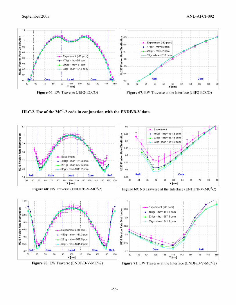
September 2003 ANL-AFCI-092
-56-
0.3
0.4
0.5
0.6
0.7
0.8
0.9
1
1.1
1.2
50 60 70 80 90 100 110 120 130 140 150Y [cm]
Np2
37 F
issi
on R
ate
Dis
trib
utio
n
Experiment (-80 pcm)471gr - rho=55 pcm299gr - rho=-81pcm33gr - rho=-1018 pcm
Refl. Core Lead Core Refl.
Figure 66: EW Traverse (JEF2-ECCO)
0.3
0.4
0.5
0.6
0.7
0.8
0.9
1
50 52 54 56 58 60 62 64 66 68 70Y [cm]
Np23
7 Fi
ssio
n R
ate
Dis
trib
utio
n
Experiment (-80 pcm)471gr - rho=55 pcm299gr - rho=-81pcm33gr - rho=-1018 pcm
Refl. Core
Figure 67: EW Traverse at the Interface (JEF2-ECCO)
III.C.2. Use of the MC2-2 code in conjunction with the ENDF/B-V data.
0.5
0.6
0.7
0.8
0.9
1
1.1
30 40 50 60 70 80 90 100 110 120 130 140 150 160 170X [cm]
U23
5 Fi
ssio
n R
ate
Dis
trib
utio
n
Experiment460gr - rho=-161.3 pcm231gr - rho=-567.5 pcm33gr - rho=-1341.2 pcm
Refl. Core Lead Core Refl.
Figure 68: NS Traverse (ENDF/B-V-MC2-2)
0.55
0.6
0.65
0.7
0.75
0.8
0.85
0.9
40 44 48 52 56 60 64 68 72 76 80X [cm]
U235
Fis
sion
Rat
e D
istr
ibut
ion
Experiment460gr - rho=-161.3 pcm231gr - rho=-567.5 pcm33gr - rho=-1341.2 pcm
Refl. Core
Figure 69: NS Traverse at the Interface (ENDF/B-V-MC2-2)
0.7
0.75
0.8
0.85
0.9
0.95
1
1.05
50 60 70 80 90 100 110 120 130 140 150Y [cm]
U23
5 Fi
ssio
n R
ate
Dis
trib
utio
n
Experiment (-80 pcm)
460gr - rho=-161.3 pcm
231gr - rho=-567.5 pcm
33gr - rho=-1341.2 pcm
Refl. Core Lead Core Refl.
Figure 70: EW Traverse (ENDF/B-V-MC2-2)
0.7
0.75
0.8
0.85
0.9
0.95
1
130 132 134 136 138 140 142 144 146 148 150Y [cm]
U23
5 Fi
ssio
n Ra
te D
istri
butio
n Experiment (-80 pcm)
460gr - rho=-161.3 pcm
231gr - rho=-567.5 pcm
33gr - rho=-1341.2 pcm
Core Refl.
Figure 71: EW Traverse at the Interface (ENDF/B-V-MC2-2)

September 2003 ANL-AFCI-092
-57-
0.3
0.4
0.5
0.6
0.7
0.8
0.9
1
1.1
1.2
50 60 70 80 90 100 110 120 130 140 150Y [cm]
Np2
37 F
issi
on R
ate
Dis
trib
utio
n
Experiment (-80 pcm)
460gr - rho=-161.3 pcm
231gr - rho=-567.5 pcm
33gr - rho=-1341.2 pcm
Refl. Core Lead Core Refl.
Figure 72: EW Traverse (ENDF/B-V-MC2-2)
0.3
0.4
0.5
0.6
0.7
0.8
0.9
1
50 52 54 56 58 60 62 64 66 68 70Y [cm]
U23
5 Fi
ssio
n Ra
te D
istri
butio
n Experiment (-80 pcm)
460gr - rho=-161.3 pcm
231gr - rho=-567.5 pcm
33gr - rho=-1341.2 pcm
Refl. Core
Figure 73: EW Traverse at the Interface (ENDF/B-V-MC2-2)
III.C.3. Use of the MC2-2 code in conjunction with the ENDF/B-VI data.
0.5
0.6
0.7
0.8
0.9
1
1.1
30 40 50 60 70 80 90 100 110 120 130 140 150 160 170X [cm]
U23
5 Fi
ssio
n R
ate
Dis
trib
utio
n
Experiment460gr - rho=464.8 pcm231gr - rho=-26.3 pcm33gr - rho=-698.5 pcm
Refl. Core Lead Core Refl.
Figure 74: NS Traverse (ENDF/B-VI-MC2-2)
0.55
0.6
0.65
0.7
0.75
0.8
0.85
0.9
40 44 48 52 56 60 64 68 72 76 80X [cm]
U235
Fis
sion
Rat
e D
istr
ibut
ion
Experiment460gr - rho=464.8 pcm231gr - rho=-26.3 pcm33gr - rho=-698.5 pcm
Refl. Core
Figure 75: NS Traverse at the Interface (ENDF/B-VI-MC2-2)
0.7
0.75
0.8
0.85
0.9
0.95
1
1.05
50 60 70 80 90 100 110 120 130 140 150Y [cm]
U23
5 Fi
ssio
n R
ate
Dis
trib
utio
n
Experiment (-80 pcm)
460gr - rho=464.8 pcm
231gr - rho=-26.3 pcm
33gr - rho=-698.5 pcm
Refl. Core Lead Core Refl.
Figure 76: EW Traverse (ENDF/B-VI-MC2-2)
0.7
0.75
0.8
0.85
0.9
0.95
1
130 132 134 136 138 140 142 144 146 148 150Y [cm]
U23
5 Fi
ssio
n Ra
te D
istri
butio
n Experiment (-80 pcm)
460gr - rho=464.8 pcm
231gr - rho=-26.3 pcm
33gr - rho=-698.5 pcm
Core Refl.
Figure 77: EW Traverse at the Interface (ENDF/B-VI-MC2-2)

September 2003 ANL-AFCI-092
-58-
0.3
0.4
0.5
0.6
0.7
0.8
0.9
1
1.1
1.2
50 60 70 80 90 100 110 120 130 140 150Y [cm]
Np2
37 F
issi
on R
ate
Dis
trib
utio
n
Experiment (-80 pcm)
460gr - rho=464.8 pcm
231gr - rho=-26.3 pcm
33gr - rho=-698.5 pcm
Refl. Core Lead Core Refl.
Figure 78: EW Traverse (ENDF/B-VI-MC2-2)
0.3
0.4
0.5
0.6
0.7
0.8
0.9
1
50 52 54 56 58 60 62 64 66 68 70Y [cm]
Np23
7 Fi
ssio
n R
ate
Dis
trib
utio
n Experiment (-80 pcm)
460gr - rho=464.8 pcm
231gr - rho=-26.3 pcm
33gr - rho=-698.5 pcm
Refl. Core
Figure 79: EW Traverse at the Interface (ENDF/B-VI-MC2-2)
III.C.4. Use of the MC2-2 code in conjunction with the JEF2.2 data.
0.5
0.6
0.7
0.8
0.9
1
1.1
30 40 50 60 70 80 90 100 110 120 130 140 150 160 170X [cm]
U23
5 Fi
ssio
n R
ate
Dis
trib
utio
n
Experiment460gr - rho=-10.6 pcm231gr - rho=-362.4 pcm33gr - rho=-952.0 pcm
Refl. Core Lead Core Refl.
Figure 80: NS Traverse (JEf2.2-MC2-2)
0.55
0.6
0.65
0.7
0.75
0.8
0.85
0.9
40 44 48 52 56 60 64 68 72 76 80X [cm]
U235
Fis
sion
Rat
e D
istr
ibut
ion
Experiment460gr - rho=-10.6 pcm231gr - rho=-362.4 pcm33gr - rho=-952.0 pcm
Refl. Core
Figure 81: NS Traverse at the Interface (JEF2.2-MC2-2)
0.7
0.75
0.8
0.85
0.9
0.95
1
1.05
50 60 70 80 90 100 110 120 130 140 150Y [cm]
U23
5 Fi
ssio
n R
ate
Dis
trib
utio
n
Experiment (-80 pcm)
460gr - rho=-10.6 pcm
231gr - rho=-362.4 pcm
33gr - rho=-952.0 pcm
Refl. Core Lead Core Refl.
Figure 82: EW Traverse (JEF2.2-MC2-2)
0.7
0.75
0.8
0.85
0.9
0.95
1
130 132 134 136 138 140 142 144 146 148 150Y [cm]
U23
5 Fi
ssio
n Ra
te D
istri
butio
n Experiment (-80 pcm)
460gr - rho=-10.6 pcm
231gr - rho=-362.4 pcm
33gr - rho=-952.0 pcm
Core Refl.
Figure 83: EW Traverse at the Interface (JEF2.2-MC2-2)

September 2003 ANL-AFCI-092
-59-
0.3
0.4
0.5
0.6
0.7
0.8
0.9
1
1.1
1.2
50 60 70 80 90 100 110 120 130 140 150Y [cm]
Np2
37 F
issi
on R
ate
Dis
trib
utio
n
Experiment (-80 pcm)
460gr - rho=-10.6 pcm
231gr - rho=-362.4 pcm
33gr - rho=-952.0 pcm
Refl. Core Lead Core Refl.
Figure 84: EW Traverse (JEF2.2-MC2-2)
0.3
0.4
0.5
0.6
0.7
0.8
0.9
1
50 52 54 56 58 60 62 64 66 68 70Y [cm]
Np23
7 Fi
ssio
n R
ate
Dis
trib
utio
n Experiment (-80 pcm)
460gr - rho=-10.6 pcm
231gr - rho=-362.4 pcm
33gr - rho=-952.0 pcm
Refl. Core
Figure 85: EW Traverse at the Interface (JEF2.2-MC2-2)
III.C.5. Effect due to the nuclear data on the adjoint flux traverses.
0.5
0.6
0.7
0.8
0.9
1
1.1
30 40 50 60 70 80 90 100 110 120 130 140 150 160 170X [cm]
U23
5 Fi
ssio
n R
ate
Dis
trib
utio
n
Experiment471gr JEF2-ECCO (55 pcm)460gr ENDF/B-V - MC2 (-161.3 pcm)460gr ENDF/B-VI - MC2 (464.8 pcm)460gr JEF2 - MC2 (-10.6 pcm)
Refl. Core Lead Core Refl.
Figure 86: NS Traverse - Nuclear Data Impact
0.6
0.65
0.7
0.75
0.8
0.85
0.9
0.95
40 44 48 52 56 60 64 68 72 76 80X [cm]
U235
Fis
sion
Rat
e D
istr
ibut
ion
Experiment471gr JEF2-ECCO (55 pcm)460gr ENDF/B-V - MC2 (-161.3 pcm)460gr ENDF/B-VI - MC2 (464.8 pcm)460gr JEF2 - MC2 (-10.6 pcm)
Refl. Core
Figure 87: NS Traverse at the Interface - Nuclear Data Impact
0.7
0.75
0.8
0.85
0.9
0.95
1
1.05
50 60 70 80 90 100 110 120 130 140 150Y [cm]
U23
5 Fi
ssio
n R
ate
Dis
trib
utio
n
Experiment (-80 pcm)471gr JEF2-ECCO (55 pcm)460gr ENDF/B-V - MC2 (-161.3 pcm)460gr ENDF/B-VI - MC2 (464.8 pcm)460gr JEF2 - MC2 (-10.6 pcm)
Refl. Core Lead Core Refl.
Figure 88: EW Traverse - Nuclear Data Impact
0.7
0.75
0.8
0.85
0.9
0.95
1
130 132 134 136 138 140 142 144 146 148 150Y [cm]
U23
5 Fi
ssio
n Ra
te D
istri
butio
n Experiment (-80 pcm)471gr JEF2-ECCO (55 pcm)460gr ENDF/B-V - MC2 (-161.3 pcm)460gr ENDF/B-VI - MC2 (464.8 pcm)460gr JEF2 - MC2 (-10.6 pcm)
Core Refl.
Figure 89: EW Traverse at the Interface - Nuclear Data Impact

September 2003 ANL-AFCI-092
-60-
0.3
0.4
0.5
0.6
0.7
0.8
0.9
1
1.1
1.2
50 60 70 80 90 100 110 120 130 140 150Y [cm]
Np2
37 F
issi
on R
ate
Dis
trib
utio
n
Experiment (-80 pcm)
471gr JEF2-ECCO (55 pcm)
460gr ENDF/B-V - MC2 (-161.3 pcm)460gr ENDF/B-VI - MC2 (464.8 pcm)
460gr JEF2 - MC2 (-10.6 pcm)
Refl. Core Lead Core Refl.
Figure 90: EW Traverse - Nuclear Data Impact
0.3
0.4
0.5
0.6
0.7
0.8
0.9
1
50 52 54 56 58 60 62 64 66 68 70Y [cm]
Np23
7 Fi
ssio
n R
ate
Dis
trib
utio
n
Experiment (-80 pcm)
471gr JEF2-ECCO (55 pcm)
460gr ENDF/B-V - MC2 (-161.3 pcm)
460gr ENDF/B-VI - MC2 (464.8 pcm)
460gr JEF2 - MC2 (-10.6 pcm)
Refl. Core
Figure 91: EW Traverse at the Interface - Nuclear Data Impact
III.D. Analysis of dynamic measurements
One of the main objectives of the MUSE-4 experimental program is to investigate the neutronic response to
neutron pulses with frequencies of 1 to 4 kHz, and less than 1µs wide, generated at the reactor center by the (d,d)
GENEPI accelerator. Detectors based on 235U and 237Np fission, located in the core, reflector and shielding
regions are used for measuring the time dependent responses.
At present only measurements for the MUSE-4 SC0 configuration (see Figure 9) are available. The axial
positioning of the control and pilot rods allowed variations in the reactivity, corresponding to different levels of
subcriticality. The following configurations have been investigated:
• MUSE-4 SC0 with pilot rod out;
• MUSE-4 SC0 with pilot rod in;
• MUSE-4 SC0 with pilot rod and control rod “bc1” in.
III.D.1. MUSE-4 SC0 with pilot rod out.
In this section, the MUSE-4 SC0 configuration with both the control rod “bc1” and the pilot rod out has been
studied (see Figure 9). The measured reactivity is -400 pcm.
In the point kinetic approximation the response P(t) to a neutron pulse is the sum of an exponential decay from
the prompt multiplication plus a nearly constant offset due to the delayed neutrons. In particular, the prompt time
dependence P(t) ~ exp(-αt), with Λ−
≅ρβα
ˆ, β the effective fraction of delayed neutron and Λ the mean
generation time characterizing the system under study, can be investigated for a method of reactivity
measurement, the Pulsed Neutron Source (PNS) method.
September 2003 ANL-AFCI-092
-61-
As a preliminary analysis, a point kinetic model has been employed for the present study using the 3D kinetic
module KIN3D [29] of the ERANOS code system [22]. The cross-sections have been processed via the ECCO
code [24] with the JEF2.2 data [23], while the MC2-2 code [25] allows the processing of ENDF/B-V and -VI and
JEF2.2 data libraries.
Due to the proximity to criticality, the best estimation for the reactivity provides positive values in some
simulations, especially when using the ENDF/B-VI data library (see Tables 4 to 7). Since the study of a system
driven by an external source requires a subcritical state, for the present analysis the calculation has been
normalized to the experimental reactivity. This choice allows also investigation of the impact of nuclear data on
the dynamic evolution of the system when the reactivity is the same in each simulation.
The results are shown in Table 16 and Figure 92.
The main problem of the PNS method consists in the limitations of the technique. Indeed, the real configuration
is often very different from a “point-reactor”, and the experimental response depends in general on the position
of the detectors.
As example, Figures 93 to 95 show the measurements associated with some detectors, located in the core
(detector F), in the reflector (detector C) and in the shielding (detector G). In order to reproduce the detector
response by the calculation, a space-time solution of the transport equation, like the direct or the quasi-static
methods (both available in KIN3D), has to be used.
In the same Figures 93 to 95, the experimental data are also compared with the calculated ones obtained with the
direct method. The use of the quasi-static approximations gives similar results. In general, the agreement with
the measurements can be considered satisfactory. Regarding the calculation, it can be observed that the effect of
using different libraries during the transient is not significant if each calculation is normalized to the same
reactivity.

September 2003 ANL-AFCI-092
-62-
Table 16: Comparison of Calculation and Experiment Results.
Experiment
ρ [pcm] β [pcm] Λ [µs]
-400 335 0.56
Calculation
JEF2.2-ECCO JEF2.2-MC2-2 ENDF/B-V-MC2-2 ENDF/B-VI-MC2-2
ρ [pcm] -400 -400 -400 -400 α [s-1] from point-model 15154.8 14999.0 15905.3 14625.7
β (t=0) [pcm] 367 371 369 376
Λ (t=0) [µs] 0.51 0.52 0.49 0.53
0.1
1
0 20 40 60 80 100 120Time [microsec.]
U5 R
elat
ive
Fiss
ion
Rate
JEF2-ECCO: KIN3D point
JEF2-MC2: KIN3D point
ENDFB5-MC2: KIN3D pointENDFB6-MC2: KIN3D point
Figure 92: Point Model Comparison
0.00
0.10
0.20
0.30
0.40
0.50
0.60
0.70
0.80
0.90
1.00
0 20 40 60 80 100 120Time [microsec.]
Det
. F (c
ore)
: U5
Fiss
. Rat
eJEF2-ECCO: KIN3D direct
JEF2-MC2: KIN3D direct
ENDFB5-MC2: KIN3D direct
ENDFB6-MC2: KIN3D direct
det F (core): Experiment
Figure 93: Detector F Comparison
0.00
0.10
0.20
0.30
0.40
0.50
0.60
0.70
0.80
0.90
1.00
0 20 40 60 80 100 120Time [microsec.]
Det
. C (r
efl.)
: U5
Fiss
. Rat
e
JEF2-ECCO: KIN3D directJEF2-MC2: KIN3D directENDFB5-MC2: KIN3D directENDFB6-MC2: KIN3D directExperiment
Figure 94: Detector C Comparison
0.00
0.10
0.20
0.30
0.40
0.50
0.60
0.70
0.80
0.90
1.00
0 20 40 60 80 100 120Time [microsec.]
Det.
G (s
hiel
d): U
5 Fi
ss. R
ate
JEF2-ECCO: KIN3D directJEF2-MC2: KIN3D direct
ENDFB5-MC2: KIN3D directENDFB6-MC2: KIN3D direct
Experiment
Figure 95: Detector G Comparison

September 2003 ANL-AFCI-092
-63-
III.D.2. MUSE-4 SC0 with pilot rod in.
In this section, the MUSE-4 SC0 configuration with the pilot rod down and the control rod “bc1” out has been
studied (see Figure 9). The measured reactivity is -540 pcm.
As a preliminary analysis, a point kinetic model has been employed for the present study using the 3D kinetic
module KIN3D [29] of the ERANOS code system [22]. The cross-sections have been processed via the ECCO
code [24] with the JEF2.2 data [23], while the MC2-2 code [25] allows the processing of ENDF/B-V and -VI and
JEF2.2 data libraries.
As in the case with pilot rod out, due to the close to criticality state, the best estimation for the reactivity
provides positive values in some simulations, especially when using the ENDF/B-VI data library (see Tables 4
to 7). Consequently, for the present analysis the calculation has been normalized to the experimental reactivity.
The results are shown in Table 17 and Figure 96.
Figures 97 to 99 show the measurements associated with some detectors, located in the core (detector F), in the
reflector (detector C) and in the shielding (detector G). In order to reproduce the detector response by the
calculation, a space-time solution of the transport equation, like the direct or the quasi-static methods (both
available in KIN3D), has to be used.
In the same Figures 97 to 99, the experimental data are also compared with the calculated ones obtained with the
direct method. The use of the quasi-static approximations gives similar results. In general, the agreement with
the measurements can be considered satisfactory. Regarding the calculation, as in the case with pilot rod out, it
can be observed that the effect of using different libraries during the transient is not significant if each
calculation is normalized to the same reactivity.

September 2003 ANL-AFCI-092
-64-
Table 17: Comparison of Calculation and Experiment Results.
Experiment
ρ [pcm] β [pcm] Λ [µs]
-540 335 0.56
Calculation
JEF2.2-ECCO JEF2.2-MC2-2 ENDF/B-V-MC2-2 ENDF/B-VI-MC2-2
ρ [pcm] -540 -540 -540 -540 α [s-1] from point-model 17886.9 17690.1 18763.1 17234.0
β (t=0) [pcm] 367 371 369 376
Λ (t=0) [µs] 0.51 0.52 0.49 0.53
0.1
1
0 20 40 60 80 100 120Time [microsec.]
U5
Rel
ativ
e Fi
ssio
n R
ate
JEF2-ECCO: KIN3D point
JEF2-MC2: KIN3D point
ENDFB5-MC2: KIN3D pointENDFB6-MC2: KIN3D point
Figure 96: Point Model Comparison
0.00
0.10
0.20
0.30
0.40
0.50
0.60
0.70
0.80
0.90
1.00
0 20 40 60 80 100 120Time [microsec.]
Det
. F (c
ore)
: U5
Fiss
. Rat
eJEF2-ECCO: KIN3D direct
JEF2-MC2: KIN3D direct
ENDFB5-MC2: KIN3D direct
ENDFB6-MC2: KIN3D direct
det F (core): Experiment
Figure 97: Detector F Comparison
0.00
0.10
0.20
0.30
0.40
0.50
0.60
0.70
0.80
0.90
1.00
0 20 40 60 80 100 120Time [microsec.]
Det
. C (r
efl.)
: U5
Fiss
. Rat
e
JEF2-ECCO: KIN3D direct
JEF2-MC2: KIN3D direct
ENDFB5-MC2: KIN3D direct
ENDFB6-MC2: KIN3D direct
Experiment
Figure 98: Detector C Comparison
0.00
0.10
0.20
0.30
0.40
0.50
0.60
0.70
0.80
0.90
1.00
0 20 40 60 80 100 120Time [microsec.]
Det.
G (s
hiel
d): U
5 Fi
ss. R
ate
JEF2-ECCO: KIN3D direct
JEF2-MC2: KIN3D direct
ENDFB5-MC2: KIN3D direct
ENDFB6-MC2: KIN3D direct
Experiment
Figure 99: Detector G Comparison

September 2003 ANL-AFCI-092
-65-
III.D.3. MUSE-4 SC0 with pilot rod and control rod bc1 in.
In this section, the MUSE-4 SC0 configuration with both the pilot rod and the control rod “bc1” in has been
studied (see Figure 9).
During the experimental phase, two values of reactivity were determined. The first is based on the Modified
Source Multiplication (MSM) method that gives a reactivity value of about –4200 pcm. Using the Pulsed
Neutrons Source (PNS) technique a reactivity value of –3200 pcm is obtained.
The MSM method determines subcritical reactivities by ratios of count rates corrected for changes in detector
efficiencies and source importance between two subcritical states. In the PNS method, information on the
subcritical level is deduced from the decay of the response P(t) arising from an external neutron pulse.
The wide discrepancy (-4200 vs. –3200 pcm) obtained using the two methods is being investigated by the
experimentalists.
As a preliminary analysis, a point kinetic model has been employed for the present study using the 3D kinetic
module KIN3D [29] of the ERANOS code system [22]. The cross-sections have been processed via the ECCO
code [24] with the JEF2.2 data [23], while the MC2-2 code [25] allows the processing of ENDF/B-V and -VI and
JEF2.2 data libraries. Because of the subcritical state, no normalization to the experimental reactivity has been
performed. The results are shown in Table 18 and Figure 100.
First, it can be seen in Table 18 that the spread in the calculated reactivity value is of the order of the difference
between the MSM and PNS inferred measurement values. It is also observed that the trend in the calculated α
value is consistent with that in the calculated subcritical level, as expected (i.e., the highest α value is obtained
for the approach with highest subcritical level).
Figures 101 to 103 show the measurements associated with some detectors, located in the core (detector F), in
the reflector (detector C) and in the shielding (detector H).
In the same Figures 101 to 103, the experimental data are also compared with the calculated ones obtained with
the direct method. The use of the quasi-static approximations gives similar results. In general, the agreement
with the measurements can be considered satisfactory. Regarding the calculation, it the can be observed that the
effect of using of different libraries during the transient becomes significant if each calculation is not normalized
to the same reactivity. We will observe that this in contrast on what has been done in section III.D. 1&2 where
the calculations were normalized to the experimental reactivity.

September 2003 ANL-AFCI-092
-66-
Table 18: Comparison of Calculation and Experiment Results.
Experiment ρ [pcm] β [pcm] Λ [µs]
-3200 (PNS) -4200 (MSM) 335 0.56 Calculation
JEF2.2-ECCO JEF2.2-MC2-2 ENDF/B-V-MC2-2 ENDF/B-VI-MC2-2ρ [pcm] -3800 -3512 -3845 -3061
α [s-1] from point-model 82530.6 76049.2 86656.2 65555.3
β (t=0) [pcm] 371 375 372 380 Λ (t=0) [µs] 0.50 0.51 0.48 0.52
0.001
0.01
0.1
1
0 20 40 60 80 100 120Time [microsec.]
U5
Rel
ativ
e Fi
ssio
n R
ate
JEF2-ECCO: KIN3D point
JEF2-MC2: KIN3D point
ENDFB5-MC2: KIN3D pointENDFB6-MC2: KIN3D point
Figure 100: Point Model Comparison
0.01
0.10
1.00
0 20 40 60 80 100 120Time [microsec.]
Det
. F (c
ore)
: U5
Fiss
. Rat
e
JEF2-ECCO: KIN3D direct
JEF2-MC2: KIN3D direct
ENDFB5-MC2: KIN3D direct
ENDFB6-MC2: KIN3D direct
det F (core): Experiment
Figure 101: Detector F Comparison
0.01
0.10
1.00
0 20 40 60 80 100 120Time [microsec.]
Det
. C (r
efl.)
: U5
Fiss
. Rat
e
JEF2-ECCO: KIN3D direct
JEF2-MC2: KIN3D direct
ENDFB5-MC2: KIN3D direct
ENDFB6-MC2: KIN3D direct
Experiment
Figure 102: Detector C Comparison
0.01
0.10
1.00
0 20 40 60 80 100 120Time [microsec.]
Det
. H (s
hiel
d): U
5 Fi
ss. R
ate
JEF2-ECCO: KIN3D direct
JEF2-MC2: KIN3D direct
ENDFB5-MC2: KIN3D direct
ENDFB6-MC2: KIN3D direct
Experiment
Figure 103: Detector H Comparison
III.D.4. The use of the PNS methods to infer the reactivity from the analysis of dynamic measurements.
Several analyses have been performed to extract information on the reactivity of the MUSE configurations [11].
In this section, preliminary studies have been devoted to the PNS method.

September 2003 ANL-AFCI-092
-67-
A first investigation has been performed in order to study any dependence of the flux response on the detector
location. The calculation confirmed that the different detector responses (235U fission rate) have approximately
the same decay slope, but the prompt-area changes significantly especially in the shielding region. This behavior
certainly raises some issues for other experimental techniques of reactivity measurement, such as the area-ratio
method, which relates the prompt to delayed area ratio with ρ/β.
Additionally, it appears that after 20 µs from the injection of the neutron pulse, i.e. when the decay becomes less
sensitive to the shape of the pulse, the detector positions indicate the same prompt time dependence (i.e. decay
slope), even if it is different from the point kinetics behavior. As an example, Figure 104 shows the case of the
SC0 configuration with control and pilot rod down (calculations made via JEF2.2-ECCO).
The use of the average Λ in the prompt decay range (from 20 to 150 µs), estimated of 7.13709E-07 sec from the
quasi-static calculation, has demonstrated that the PNS method could still apply. In fact, the technique leads to a
reactivity determination of about –3550 pcm that is quite independent from the detector position (see Table 19)
and in reasonable agreement with the absolute calculated value (-3800 pcm). Further investigations are needed
on this aspect.
y = 1.03904e-7.12061E-2t
y = 3.94309E-1e-5.48620E-2t
y = 6.41930E-1e-5.40101E-2t
y = 1.48170E-1e-5.59803E-2t
1E-6
1E-5
1E-4
1E-3
1E-2
1E-1
1E+0
20 40 60 80 100 120Time [microsec.]
Flux
det I det Ddet G pointExp. (point) Expon. (det D)Expon. (det G) Expon. (det I)
Figure 104: C-E Comparison.

September 2003 ANL-AFCI-092
-68-
Table 19: Estimated (JEF2.2-ECCO) Reactivity by the PNS Method at Different Detector Locations.
detector α β Average Λ Reactivity deduced with the PNS method
I (core) 5.59803E+4 370.59 pcm 7.13709E-07 sec -3620 pcm
D (reflector) 5.48620E+4 370.59 pcm 7.13709E-07 sec -3540 pcm
G (shielding) 5.40101E+4 370.59 pcm 7.13709E-07 sec -3480 pcm

September 2003 ANL-AFCI-092
-69-
IV. MUSE-4 Benchmark
IV.A. Introduction
The study of the neutronics of ADS, in which an intense neutron source maintains a stationary power level,
requires the extension of standard computational tools developed for critical reactors to solve steady-state and
time–dependent problems. With this goal, the experiment MUSE-4 [7,8] (using the MASURCA reactor) became
the object of the benchmark [10] proposed by OECD for the validation of the neutronic tools (codes and cross
section data) to be used for the ADS design.
The benchmark model is oriented to compare simulation predictions based on available codes and nuclear data
libraries with experimental data related to: TRU transmutation, criticality constants and time evolution of the
neutronic flux following source variation, within “liquid” metal fast subcritical systems.
The benchmark has been divided in three steps. The first step will allow an understanding of the physics
methods using different groups and tuning of the analysis programs with the experimental data of an already
measured configuration (COSMO). In the second step, the MUSE-4 reference configuration (1112 cells) is
proposed to simulate different reactor parameters (criticality constant, flux distribution...) in a nearly critical
configuration. Finally, a third step is oriented to the simulation of reactor response to the external source in the
subcritical reference configuration (976 cells).
Note that MASURCA can be operated in two modes. In the (nearly) critical configurations the intrinsic (Pu
decay) neutron source plus an initial external source initiate a level of neutron flux that is afterwards maintained
by reactivity control mechanisms. The neutron flux in MASURCA is in a very good approximation an
eigenvector of the transport equation. In the two first steps of the requested calculations (COSMO and 1112 cells
MUSE-4 reference configuration) the flux is assumed to be computed as the transport equation eigenvector. In
the second mode of operation, with low values of the multiplication constant, the flux reaches rapidly the
equilibrium value corresponding to the intrinsic source multiplied by the subcritical system. That equilibrium
value is small (assumed negligible) and the main part of the neutron flux must be produced by the multiplication
of an external deuterium-tritium neutron source placed near the MASURCA center.
IV.B. Geometry and material description.
The MASURCA facility is an arrangement of tubes of 10.6 × 10.6 × 164.16 cm3 each, building a parallel-piped
assembly of 17 × 16 tubes, with a total dimension of 180.2 × 169.6 × 164.16 cm3 in the MUSE-4 configurations
and 17 × 17 tubes in the COSMO configuration.

September 2003 ANL-AFCI-092
-70-
Figures 101 to 103 show the layout of MASURCA facility for the COSMO configuration. Figures 104 to 106
show the critical reference and Figure 107 the subcritical configuration for the MUSE-4 experiments. Figures
108 and 109 show the axial view of the different types of MUSE-4 tubes, including the material labels. It should
be noted that tubes 3* and 11* can be obtained rotating tubes 3 and 11 by 180° around its vertical (Z) axis. Tube
9* can be obtained rotating tube 9 to 90°, 180° or 270°, tube 12* can be obtained by rotating 270° tube 12, and
tube 10** can be obtained as a mirror image of tube 10.
Detector positions are shown in Figure 110. All vertical channels are in the center of the tube. Note that
horizontal and vertical channels are not included in the geometrical description in order to simplify the model.
Figure 105: COSMO Configuration – Top View at Half Height
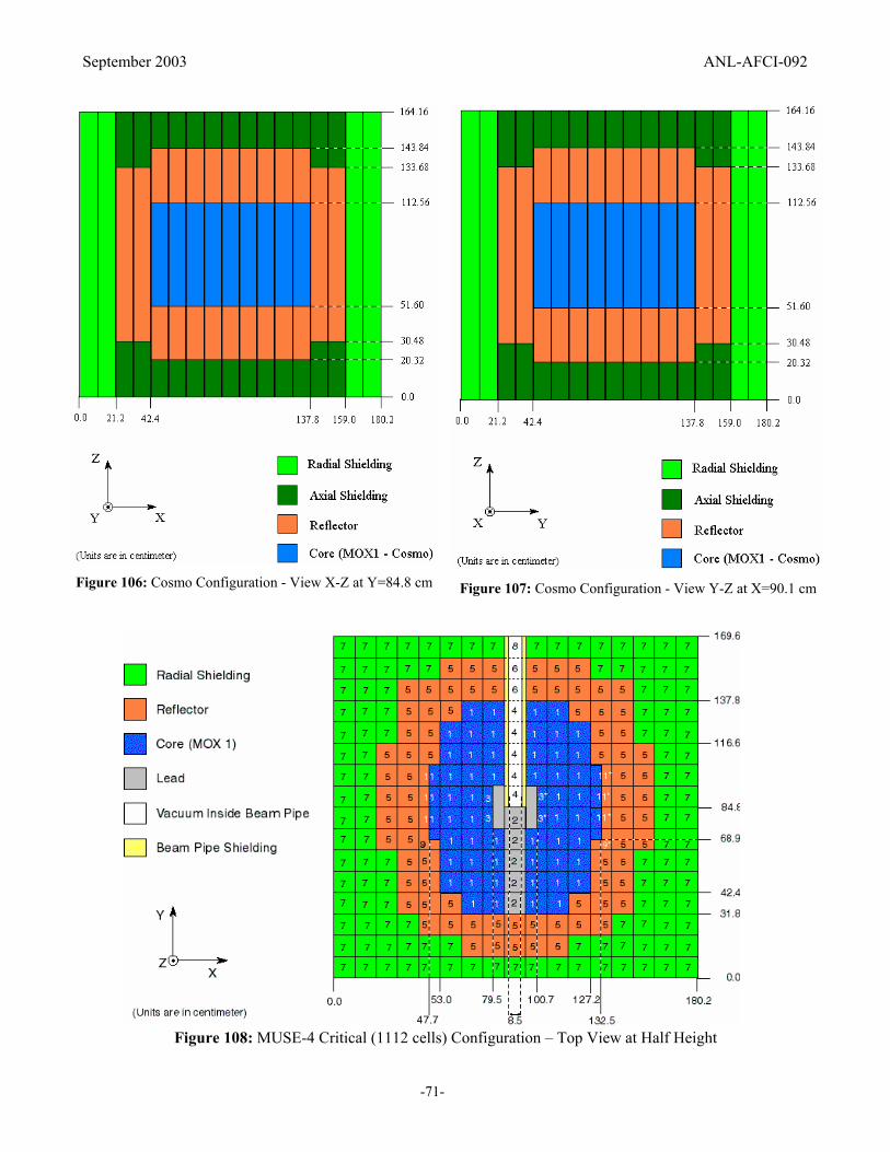
September 2003 ANL-AFCI-092
-71-
Figure 106: Cosmo Configuration - View X-Z at Y=84.8 cm Figure 107: Cosmo Configuration - View Y-Z at X=90.1 cm
Figure 108: MUSE-4 Critical (1112 cells) Configuration – Top View at Half Height

September 2003 ANL-AFCI-092
-72-
Figure 109: MUSE-4 Critical Config. – Side View #1 at Y=90.1 cm
Figure 110: MUSE-4 Critical Config. – Side View #2 at X=90.1 cm
Figure 111: Configuration MUSE-4 976 Cells – Top View at Half Height

September 2003 ANL-AFCI-092
-73-
Figure 112: Axial View of the MUSE-4 Tubes 1 to 8 and 11
Figure 113: Axial View of the MUSE-4 Tubes 4 and 9

September 2003 ANL-AFCI-092
-74-
Figure 114: Detector Position
IV.C. Requested calculations
IV.C.1. COSMO calculations
1. Criticality constant, keff, for the COSMO configuration.
2. 235U, 237Np fission rate and 10B (n,α) relative to Y = 90 cm 235U fission in the following channels:
Horizontal channel at X = 82.89 cm and Z = 81.48 cm for: Y = 40, 50, 60, 70, 80, 90, 100, 110, 120, 130,
140 cm.
X =90.1 cm, Y = 90.1 cm and Z = 82.08 cm for all of them and Z = 42, 52, 62, 72, 92, 102, 112, 122 cm
for 237Np.
3. Fission reaction rates ratios of 238U, 238Pu, 239Pu, 240Pu, 241Pu, 242Pu, 241Am, 243Am, and capture in 55Mn, 115In, 197Au always relative to 235U fission at the following positions:
Position 1. X = 82.89 cm, Y = 90.1 cm and Z = 81.48 cm.
Position 2. X =90.1 cm, Y = 90.1 cm and Z = 82.08 cm.
4. Relative neutron spectrum in the same positions as point 3, normalized in such way that the integral will be
1. ERANOS 172 energy bins format and optionally an additional free energy binning are requested.

September 2003 ANL-AFCI-092
-75-
IV.C.2 Critical MUSE-4 reference configuration calculations
1. Criticality constant, keff, for the MUSE-4 1 112-cell reference configuration.
2. 235U fission rate as a function of the position in the following channels:
Horizontal channel E-W at Y = 86.71 cm and Z = 72.52 cm for: X = 5, 15, 25, 35, 45, 55, 65, 75, 85,
95, 90.1, 105, 115, 125, 135, 145, 155, 165, 175 cm.
Horizontal channel N-S at X = 82.89 cm and Z = 81.48 cm for: Y = 40, 50, 60, 70, 80, 90, 100, 110,
120, 130, 140 cm.
Vertical channels C7 (X = 90.1 cm, Y = 79.5 cm) and C9 (X = 68.9 cm, Y = 58.3 cm) at Z = 32, 42, 52,
62, 72, 82, 92, 102, 112, 122, 132 cm.
All data normalized at the vertical channel C7 at position Z = 82 cm.
3. Reaction rates ratios of fission and capture in 238U, 238Pu, 239Pu, 240Pu, 241Pu, 242Pu, 241Am, 243Am, and capture
in 55Mn, 115In, 197Au at the center of the E-W, N-S and vertical channels c7 and c9, relative to 235U fission, at
c7 (X = 90.1 cm, Y = 79.5 cm) at position Z = 82 cm. Find co-ordinates on the attached tables for result
reporting.
4. Relative neutron fluence spectrum in the same positions as point 3, normalized in such way that the integral
will be 1. ERANOS 172 energy bins format and optionally an additional free energy binning are requested.
5. Mean neutron lifetime l and βeff.
IV.C.3. Subcritical configuration calculations
1. Reactivity change between reference 1 112-cell configuration and 976-cell configuration of MUSE-4.
( ) ( )∆k k conf cells k conf ref cellseff eff eff= −. . .976 1 112
2. 235U fission rate as a function of the position in the following channels:
Horizontal channel E-W at Y = 86.71 cm and Z = 72.52 cm for: X = 5, 15, 25, 35, 45, 55, 65, 75, 85,
90.1, 95, 105, 115, 125, 135, 145, 155, 165, 175 cm.
Horizontal channel N-S at X = 82.89 cm and Z = 81.48 cm for: Y = 40, 50, 60, 70, 80, 90, 100, 110,
120, 130, 140 cm.
Vertical channel C7 and C9 at Z = 32, 42, 52, 62, 72, 82, 92, 102, 112, 122, 132 cm.
All data normalised at the vertical channel C7 at position Z = 82 cm.
3. Reaction rates ratios of fission and capture in 238U, 238Pu, 239Pu, 240Pu, 241Pu, 242Pu, 241Am, 243Am, and
capture in 55Mn, 115In, 197Au at the centre of the E-W, N-S and vertical channels, relative to 235U fission.
Find co-ordinates on the attached tables for result reporting.

September 2003 ANL-AFCI-092
-76-
4. Relative neutron spectrum in the same positions as point 3, normalized in such way that the integral will be
1. ERANOS 172 energy bins format and optionally an additional free energy binning are requested.
5. 235U fission rate as a function of the time after the deuteron-tritium source pulse in the fixed detectors A, B,
C, D, F, G, H, I and L, at Z = 95 cm, normalized in such a way to make maximum of each channel equal to
1. The deuteron beam is assumed to have a time structure of 1 µs pulses repeated at 1 kHz. The time step and
range will be of 1 µs and 500 µs respectively. Calculation is requested for pulse #1 and for pulse after
equilibrium (n → ∞).
6. Mean neutron lifetime l and βeff.
7. Difference between keff and ksource for the 976-cell MUSE-4 configuration. ksource is defined by:
sourcekneutronssourceofnumberTotal
dtransporteneutronsofnumberTotal−
=1
1
An equivalent definition is provided by the equation (⟨⟩ denotes integrated quantities):
( )
( )
( )
( )∑
∑
∑
∑Φ∇⋅Ω+ΦΣ+ΦΣ+ΦΣ
ΦΣ+ΦΣ=
ΦΣ+ΦΣ+
ΦΣ+ΦΣ=
xxnnfc
xxnnff
xxnnff
xxnnff
sourcex
x
xS
xk
,
,
,
, ν
ν
ν
where S is the source strength.
8. Total time-averaged power produced in the MUSE subcritical core for an average pulse intensity of 107
neutrons per pulse and a repetition rate of 1 KHz.
IV.D. Calculations details.
The requested calculations have been performed using both the ERANOS [22] deterministic code system and
VIM [30] probabilistic (Monte-Carlo) code. The VIM application has been limited to the Benchmark STEP 2
(MUSE-4 critical reference configuration).
• The basic data for the deterministic calculations have been taken from JEF2.2 [23], ENDF/B-V and
ENDF/B-VI libraries. The cross sections have been processed using both ECCO [24] (with JEF2.2) and
MC2-2 [25] (with ENDF-B/V, ENDF-B/VI and JEF2.2) codes. The eigenvalue calculations have been
performed via VARIANT [26] (3D nodal transport code), implemented in the ERANOS code system.
Finally, the dynamic calculations related to the STEP 3 have been carried out with the KIN3D code [29].
The Cell Calculation has been carried out as follows:
a) Resonance treatment:

September 2003 ANL-AFCI-092
-77-
MC2-2: Fast and accurate resonance integral methods are used in the narrow resonance resolved and
unresolved resonance treatments.
ECCO: Subgroup method and probability tables.
b) A weighted fission spectrum from mix of all fissile nuclides with iterative procedure was used.
c) The (n,2n) is included in scattering matrix.
d) The weighting spectrum for scattering matrices is standard weighting using ultra-fine group spectrum.
e) Method used for spectrum calculation, treatment of leakage in MC2-2 and ECCO:
The extended transport P1, B1, consistent P1, and consistent B1 fundamental mode ultra-fine-group
equations are solved using continuous slowing-down theory and multigroup methods.
Leakage is calculated as a DB2 term for core fundamental mode calculations. For non fissile
compositions a leakage terms is derived from core and used as a source.
f) The number of energy groups used in the different calculation phases change as follows:
MC2-2: 2082 groups. ECCO: 1968 groups. VARIANT: 2082 or 1968 groups for eigenvalue
calculations and 460 groups for reaction rate distribution and spectrum calculations.
• The cross section data for Monte Carlo (VIM) calculations have been taken from ENDF/B-VI. The
eigenvalue calculations were completed using ENDF/B-V and JEF-2.2 libraries.
No cell calculation for Monte Carlo code: the library is continuous energy.
For the eigenvalue calculations (JEF-2.2, ENDF/B-V) the following parameters have been used:
5000 histories per generation; 20 generations skipped before scoring, then 100 generations.
Monte Carlo parameters for the four traverse calculations:
5000 histories per generation; 20 generations skipped before scoring, then 1000 generations.
Geometric splitting using a factor of 3 across two nested rectangular surfaces 5 and 10 cm from the axes of
the foil locations, respectively, to improve efficiency, one calculation for each traverse (E-W, N-S, C7, and
C9). To reduce further the uncertainty in the reaction rates in the center foil in the C7 fuel element,
geometric splitting across three nested cubic surfaces was applied, also with a factor of 3 across each
surface.
Spectrum: The group fluxes are the integral over each group of the scalar flux (not flux per unit energy or
lethargy), so integration over energy is merely the sum of the group fluxes.
Other observations: keff was not different when the AG3 was smeared in the vacuum it surrounds.

September 2003 ANL-AFCI-092
-78-
IV.E. MUSE-4 benchmark revised calculations
In this section the results of revised calculations are reported concerning the reactivity value of the three
configurations when using the MC2-2 code to process the cross sections and the dynamic study for the subcritical
configuration. The details and the results of the other requested calculations have been already presented in the
Ref. 12.
IV.E.1. Reactivity results
Criticality constant Keff (final results):
ERANOS:
JEF2.2-ECCO-VARIANT: Keff = 1.00071 (ρ = 71 pcm)
ENDF/B-V – MC2-2 – VARIANT: Keff = 1.00026 (ρ = +26 pcm)
ENDF/B-VI – MC2-2 – VARIANT: Keff = 1.00817 (ρ = +810 pcm)
JEF2.2 – MC2-2 – VARIANT: Keff = 1.00360 (ρ = +359 pcm)
VIM:
JEF2.2: Keff = 1.00436 ± 0.0009 (ρ = 439 ± 90 pcm)
ENDF/B-V: Keff = 1.0037 ± 0.0010 (ρ = 369 ± 100 pcm)
ENDF/B-VI: Keff = 1.0052 ± 0.0009 (ρ = 517 ± 90 pcm)
The ERANOS results have been obtained in four steps. In the following we report the details for the case
JEF2.2-ECCO, keeping in mind that a similar approach has been also used for the MC2-2 calculations.
Step 1: investigation of the change on the reactivity results through the number of energy groups (NG) used.
This dependence has been quoted for NG increasing from 33 up to 838.
Table 20: MUSE-4 Critical Configuration - Keff ECCO - VARIANT JEF2.2 - ECCO
NG VARIANT(1) - ERANOS: Keff ρ [pcm]
33(2) .98664 -1354 172(2) .98933 -1079 231(2) .99389 -615 471(2) .99695 -306 838(2) .99815 -185
(1) Flux and leakage expansion order 3 WITH SIMPLIFIED SPHERICAL HARMONIC (HS) (2) With condensation from a fine step to NG
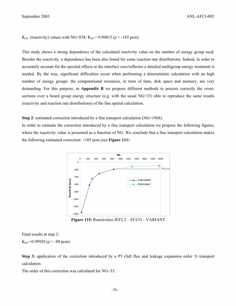
September 2003 ANL-AFCI-092
-79-
Keff (reactivity) values with NG=838: Keff = 0.99815 (ρ = -185 pcm)
This study shows a strong dependence of the calculated reactivity value on the number of energy group used.
Besides the reactivity, a dependence has been also found for some reaction rate distributions. Indeed, in order to
accurately account for the spectral effects at the interface core/reflector a detailed multigroup energy treatment is
needed. By the way, significant difficulties occur when performing a deterministic calculation with an high
number of energy groups: the computational resources, in term of time, disk space and memory, are very
demanding. For this purpose, in Appendix B we propose different methods to process correctly the cross-
sections over a board group energy structure (e.g. with the usual NG=33) able to reproduce the same results
(reactivity and reaction rate distributions) of the fine spatial calculation.
Step 2: estimated correction introduced by a fine transport calculation (NG=1968).
In order to estimate the correction introduced by a fine transport calculation we propose the following figures,
where the reactivity value is presented as a function of NG. We conclude that a fine transport calculation makes
the following estimated correction: +105 pcm (see Figure 111)
-1400
-1200
-1000
-800
-600
-400
-200
00 200 400 600 800 1000 1200 1400 1600 1800 2000
NG
Rea
ctiv
ity [p
cm] Calculated
Estimated
105 pcm
Figure 115: Reactivities JEF2.2 – ECCO – VARIANT
Final results at step 2:
Keff =0.99920 (ρ = -80 pcm)
Step 3: application of the correction introduced by a P3 (full flux and leakage expansion order 3) transport
calculation.
The order of this correction was calculated for NG=33:

September 2003 ANL-AFCI-092
-80-
Table 21: MUSE-4 Critical Config. - Transport P3 (Full Flux and Leakage Expansion Order 3) Correction MUSE-4 Critical – NG=33 HS: ρ [pcm] P3: ρ [pcm] ∆ρ = P3 - HS
JEF2.2 – ECCO -1354 -1283 +71
Final results at step 3 by application of the correction shown on column 4:
Keff = 0.99991 (ρ = -9 pcm)
Step 4: application of the correction introduced by the P3 anisotropic scattering order 3 transport calculation.
The order of this correction was calculated for NG=33:
Table 22: MUSE-4 Critical Configuration - Anisotropic Order 3 Transport Correction MUSE-4 Critical – NG=33 P1: ρ [pcm] P3: ρ [pcm] ∆ρ = P3 – P1
JEF2.2 – ECCO -1354 -1274 +80
Final results at step 4 by application of the correction shown on column 4:
Keff = 1.00071 (ρ = 71 pcm)
Important. Originally the MC2-2 results provided the following results:
Table 23: MUSE-4 Critical Configuration - Keff MC2-2 - VARIANT ENDF/B-V – MC2-2 ENDF/B-VI – MC2-2 JEF2.2 – MC2-2
NG VARIANT(1) - ERANOS: Keff ρ [pcm]
VARIANT(1) - ERANOS: Keff ρ [pcm]
VARIANT(1) - ERANOS: Keff ρ [pcm]
33(2) 1.01554 1530 1.02346 2292 1.02358 2304 231(2) 1.01105 1093 1.01757 1727 1.01605 1580 460(2) 1.00759 753 1.01440 1420 1.01185 1171 887(2) 1.00639 635 1.01278 1262 1.01032 1021
(1) Flux and leakage expansion order 3 WITH SIMPLIFIED SPHERICAL HARMONIC (HS) (2) With condensation from a fine step to NG
the application of the same procedure as described above lead to the following best estimated results:
ENDF/B-V – MC2-2 – VARIANT: Keff = 1.00718 (ρ = +713 pcm)
ENDF/B-VI – MC2-2 – VARIANT: Keff = 1.01361 (ρ = +1343 pcm)
JEF2.2 – MC2-2 – VARIANT: Keff = 1.01066 (ρ = +1055 pcm)

September 2003 ANL-AFCI-092
-81-
The most evident issue is the huge discrepancy observed for the 33-group calculation between the ECCO and
MC2-2 results. An in-depth analysis has been carried out and we concluded that this discrepancy is due to an
inconsistency in the MC2-2 code when processing the total cross-section. Indeed, the solution of the Boltzmann
equation with a deterministic multigroup PN approximation can use the total cross-section weighted with the
flux, the current or in a general case with an high order moment Φn (n >1) of the flux expansion in Legendre’s
Polynomials, but in order to proceed consistently with this choice an appropriate correction is to be introduced
on the within-group scattering cross-section. The details are given in Appendix A.
After correction, the results given in Table 22 change as follows:
Table 24: MUSE-4 Critical Configuration - Keff MC2-2 - VARIANT ENDF/B-V – MC2-2 ENDF/B-VI – MC2-2 JEF2.2 – MC2-2
NG VARIANT(1) - ERANOS: Keff ρ [pcm]
VARIANT(1) - ERANOS: Keff .ρ [pcm]
VARIANT(1) - ERANOS: Keff ρ [pcm]
33(2) 0.98075 -1963 0.98804 -1210 0.98514 -1508 231(2) 0.99141 -866 0.99819 -181 0.99522 -480 460(2) 0.99535 -467 1.00283 282 0.99874 -126 887(2) 0.99776 -225 1.00538 535 1.00131 131
(1) Flux and leakage expansion order 3 WITH SIMPLIFIED SPHERICAL HARMONIC (HS) (2) With condensation from a fine step to NG
With the same approach, the reactivity results for the other configurations proposed in the benchmark have been
revised as follows:
• COSMO configuration
ERANOS:
JEF2.2-ECCO-VARIANT: Keff = 1.00190 (ρ = 190 pcm)
ENDF/B-V – MC2-2 – VARIANT: Keff = 1.00216 (ρ = 216 pcm)
ENDF/B-VI – MC2-2 – VARIANT: Keff = 1.00921 (ρ = 913 pcm)
JEF2.2 – MC2-2 – VARIANT: Keff = 1.00478 (ρ = 476 pcm)
• MUSE-4 Subcritical Configuration
ERANOS:
JEF2.2-ECCO-VARIANT: Keff = 0.96863 (ρ = -3239 pcm)
ENDF/B-V – MC2-2 – VARIANT: Keff = 0.96796 (ρ = -3310 pcm)
ENDF/B-VI – MC2-2 – VARIANT: Keff = 0.97564 (ρ = -2497 pcm)
JEF2.2 – MC2-2 – VARIANT: Keff = 0.97188 (ρ = -2893 pcm)

September 2003 ANL-AFCI-092
-82-
IV.E.2. Dynamic results
The cooperation with Andrei Rineisky from FZK-Karlsruhe (Germany) led to the final dynamic results of the
point 5 of the MUSE4 Benchmark - Step 3 (MUSE4 subcritical configuration). In particular the response of the
detectors in the shielding and in the reflector has been improved. The Figure 112 shows the new results obtained
with KIN3D for each detector and the Figures 117 and 128 show each detector response separately with the
comparison with the other Monte-Carlo results when available. We can observe that the agreement with the
other attendants to the Benchmark, using for the most part a Monte-Carlo code, is now very good.
1.0E-5
1.0E-4
1.0E-3
1.0E-2
1.0E-1
1.0E+0
0.0E+0 5.0E-5 1.0E-4 1.5E-4 2.0E-4 2.5E-4 3.0E-4Time [sec.]
U235
Fis
sion
Rat
e
Det. FDet. IDet. LDet. CDet. ADet. JDet. GDet. H
Figure 116: KIN3D Direct Method – All Detector Behaviors

September 2003 ANL-AFCI-092
-83-
Figure 117: Detector I – Monte-Carlo Results
1.0E-5
1.0E-4
1.0E-3
1.0E-2
1.0E-1
1.0E+0
0.0E+0 5.0E-5 1.0E-4 1.5E-4 2.0E-4 2.5E-4 3.0E-4Time [sec.]
U23
5 Fi
ssio
n R
ate Det. I
Figure 118: Detector I – KIN3D
Figure 119: Detector F – Monte-Carlo Results
1.0E-5
1.0E-4
1.0E-3
1.0E-2
1.0E-1
1.0E+0
0.0E+0 5.0E-5 1.0E-4 1.5E-4 2.0E-4 2.5E-4 3.0E-4Time [sec.]
U23
5 Fi
ssio
n R
ate Det. F
Figure 120: Detector F – KIN3D
1.0E-5
1.0E-4
1.0E-3
1.0E-2
1.0E-1
1.0E+0
0.0E+0 5.0E-5 1.0E-4 1.5E-4 2.0E-4 2.5E-4 3.0E-4Time [sec.]
U23
5 Fi
ssio
n R
ate Det. L
Figure 121: Detector L – KIN3D

September 2003 ANL-AFCI-092
-84-
1.0E-5
1.0E-4
1.0E-3
1.0E-2
1.0E-1
1.0E+0
0.0E+0 5.0E-5 1.0E-4 1.5E-4 2.0E-4 2.5E-4 3.0E-4Time [sec.]
U23
5 Fi
ssio
n Ra
te
Det. C
Figure 122: Detector C – KIN3D
Figure 123: Detector A – Monte-Carlo Results
1.0E-5
1.0E-4
1.0E-3
1.0E-2
1.0E-1
1.0E+0
0.0E+0 5.0E-5 1.0E-4 1.5E-4 2.0E-4 2.5E-4 3.0E-4Time [sec.]
U235
Fis
sion
Rat
e
Det. A
Figure 124: Detector A – KIN3D
1.0E-5
1.0E-4
1.0E-3
1.0E-2
1.0E-1
1.0E+0
0.0E+0 5.0E-5 1.0E-4 1.5E-4 2.0E-4 2.5E-4 3.0E-4Time [sec.]
U23
5 Fi
ssio
n Ra
te
Det. J
Figure 125: Detector J – KIN3D

September 2003 ANL-AFCI-092
-85-
Figure 126: Detector G – Monte-Carlo Results
1.0E-7
1.0E-6
1.0E-5
1.0E-4
1.0E-3
1.0E-2
1.0E-1
1.0E+0
0.0E+0 5.0E-5 1.0E-4 1.5E-4 2.0E-4 2.5E-4 3.0E-4Time [sec.]
U235
Fis
sion
Rat
e
Det. G
Figure 127: Detector G – KIN3D
1.0E-7
1.0E-6
1.0E-5
1.0E-4
1.0E-3
1.0E-2
1.0E-1
1.0E+0
0.0E+0 5.0E-5 1.0E-4 1.5E-4 2.0E-4 2.5E-4 3.0E-4Time [sec.]
U235
Fis
sion
Rat
e
Det. H
Figure 128: Detector H – KIN3D

September 2003 ANL-AFCI-092
-86-
V. Conclusions
This report has presented a review of the activities performed by the five teams involved in the MUSE-4
experimental program. More details about the contribution provided by ANL during the year 9/02 to 9/03 has
been presented (see Ref. 12 for an accurate description of the previous work). The ANL activity consisted both
in direct participation in the experimental measurements in particular with the assistance given by G. Imel
currently at CEA-CADARACHE and in the analysis by the calculation of the experimental data.
The analysis has been focused on the subcritical level determination, on adjoint flux and fission rate traverses, on
the dynamic measurements.
The following observations have been made:
• Reactivity calculation.
The study shows a strong dependence of the calculated reactivity value on the number of energy groups
used. Indeed, in order to accurately account for the spectral effects at the interface core/reflector a detailed
multigroup energy treatment is needed. Significant difficulties occur when performing a deterministic
calculation with an high number of energy groups: the computational resources, in term of time, disk space
and memory, are very demanding. For this purpose, different methods have been proposed in order to
process correctly the cross-sections over a board group energy structure (e.g. with the usual NG=33), able to
reproduce the same results (reactivity and reaction rate distributions) of the fine spatial calculation.
The impact on the reactivity calculation due to the use of different nuclear data can be observed when the
cross-sections are processed with the MC2-2 code: moving from the ENDF/B-V to the ENDF/B-VI library
causes a spread on the reactivity results of about 700 pcm. While the comparison between the JEF2.2-ECCO
and JEF2.2- MC2-2 results allows to estimate the effect due to the use of different codes (ECCO vs MC2-2)
when the nuclear data are the same: this effect is of about 150 pcm.
The experiment-calculation discrepancy observed on the reactivity values fit well within the margin of the
uncertainty in the cases JEF2.2-ECCO and ENDF/B-V - MC2-2 (∆ ρ = 177 and 17 pcm respectively). Some
difficulties appear when using the MC2-2 code in conjunction with the JEF2.2 and ENDF/B-VI data.
However, among the sources of uncertainties there is of course also the uncertainty associated to the nuclear
data that has not been considered in the present analysis.

September 2003 ANL-AFCI-092
-87-
• Adjoint flux distributions
The analysis of the experimental traverses with californium source for the MUSE-4 reference configuration
has been performed. These traverses represent the adjoint flux distribution. The axial traverses have been
performed at the positions E1615, E1818, W2018 and W2217. The positions E1615 and W2217 are
relatively unperturbed, while the position E1918 is in the lead buffer zone and W2018 is near both to the
lead buffer zone and to a control rod. The traverses were made at two reactivity levels: roughly –70 pcm
with the pilot rod (PR) down and roughly –20 pcm with the PR at 600 mm. North-South (NS) and East-West
(EW) radial traverses were also performed for the two reactivities.
The calculation results show that the model does not accurately fit the adjoint flux outside the core when
only 33 energy groups are used. The model consistently underestimates the adjoint flux in all the traverses.
Indeed, a correct description of the slowing down of the neutrons and their reflection in the fuel at the
interface core/reflector, needs the use of an higher number of energy groups NG.
The discrepancies are sharply reduced when NG increases. In this case, the calculations performed for
example via JEF2.2-ECCO with NG = 299, 471, 838 show approximately the same results, consequently a
299 energy group structure seems to be enough for the analysis of the experimental data. The same remark
applies when the MC2-2 code is used, but in this case 231 energy groups are employed instead of 299. Using
299 (or 231) energy groups the model still underestimates the adjoint flux, but the observed discrepancies
seem to be within the margins if an uncertainty associated to the calculation would be taken in account
together with the experimental one.
All the measured traverses have been studied, but in the document just the adjoint flux distributions observed
with pilot rod (PR) at 600 mm are discussed. Indeed, with PR inserted the measured and calculated results
are about the same; slight differences appear just in the case of the E1918 traverse which is at the same time
close to a control rod and it is also the closest traverse to the PR.
The use of different nuclear data libraries doesn’t seem to affect the calculated adjoint flux distributions if
the same number of energy group is used.
However, an asymmetry is observed in some data that is not seen in the model. This is especially true for the
W2018H traverses, but it also appears for the E1918H traverse. At the present time, it is not clear whether
the asymmetries seen in the data correspond to a real physical effect, or they are due to some bias.
• Fission rate traverses.
U235 fission radial traverses EW and NS, and the Np237 EW radial traverse of the MUSE-4 critical
configuration (1115 cells) have been calculated.
In general, all the traverses show a good agreement between the calculation and the experiment in the
margin of the uncertainty on the measurement if the number of energy group is sufficiently high. For the NS

September 2003 ANL-AFCI-092
-88-
traverse a 2.5 cm translation has been applied. For the U5 EW traverse an uncertainty too large on the
experimental values has been provided, consequently a value of 2% has been used.
A good agreement between the calculation and the experiment is also found in proximity of the reflector. In
the case of the NS traverse this agreement decreases because of the proximity of the void region too.
Concerning the impact of the nuclear data on the calculated traverses, the MC2-2 – ENDF/B-VI calculation
overestimates the other simulations.
• Dynamic calculations
During the MUSE-4 phase of the experimental program, one of the objectives is to investigate the neutronic
response to neutron pulses with frequencies of 1 to 4 kHz, and less than 1µs wide, generated at the reactor
center by the (d,d) GENEPI accelerator. Detectors based on 235U and 237Np fission, located in the core,
reflector and shielding regions are used for measuring the time dependent responses.
Measurements are available for the MUSE-4 SC0 configuration. The axial positioning of the control and
pilot rods allowed to produce different core configurations, corresponding to different levels of
subcriticality. The following configurations have been investigated:
• MUSE-4 SC0 with pilot rod out;
• MUSE-4 SC0 with pilot rod in;
• MUSE-4 SC0 with pilot rod and control rod “bc1” in.
In the point kinetic approximation the response P(t) to a neutron pulse is the sum of an exponential decay
from the prompt multiplication plus a nearly constant offset due to the delayed neutrons. In particular, the
prompt time dependence P(t) ~ exp(-αt), with Λ−
≅ρβα
ˆ, β the effective fraction of delayed neutron and Λ
the mean generation time characterizing the system under study, can be investigated for a method of
reactivity measurement, the Pulsed Neutron Source (PNS) method.
As a preliminary analysis, a point kinetic model has been employed for the present study.
Due to the proximity to critical state of the configurations with pilot rod in and out, since the best estimation
for the reactivity provides positive values in some simulations, especially when using the ENDF/B-VI data
library, the calculation has been normalized to the experimental reactivity (indeed, the study of a system
driven by an external source requires a subcritical state). Instead, in the case of the configuration with
control rod bc1 in, no normalization has been performed.
The main problem of the PNS method consists in the limitations of the technique. Indeed, the real
configuration is often very different from a “point-reactor”, and the experimental response depends in
general on the position of the detectors. In order to reproduce the detector response by the calculation, a

September 2003 ANL-AFCI-092
-89-
space-time solution of the transport equation, like the direct or the quasi-static methods (both available in
KIN3D), has to be used.
In general, the agreement with the measurements has been found satisfactory for each configuration
analyzed. Regarding the calculation, it can be observed that the effect due to the use of different libraries
during the transient is not significant if each calculation is normalized to the same reactivity. Instead, the
effect is important if no normalization is performed.
Several analyses have been performed to extract information on the reactivity of the MUSE configurations,
in particular using the PNS method.
A first investigation has been performed to study any dependence of the flux response on the detector
location. The calculation confirmed that the different detector responses (235U fission rate) have
approximately the same decay slope, but the prompt-area changes significantly especially in the shielding
region. This behavior certainly raises some issues for other experimental techniques of reactivity
measurement, such as the area-ratio method, which relates the prompt to delayed area ratio with ρ/β.
Additionally, it appears that after 20 µs from the injection of the neutron pulse, i.e. when the decay becomes
less sensitive to the shape of the pulse, the detector positions indicate the same prompt time dependence (i.e.
decay slope), even if it is different from the point kinetics behavior. It has been demonstrated that using an
average Λ in the prompt decay range (from 20 to 150 µs), the PNS method could still apply. Further
investigations are needed on this aspect.
Besides the analysis of the experimental data, the MUSE-4 benchmark proposed by the OECD has been
completed.
The benchmark has been divided in three steps. The first step allows an understanding of the analysis methods of
the different groups and tuning of the simulation programs with the experimental data of an already measured
configuration (COSMO). In the second step, the MUSE-4 reference configuration (1112 cells) is proposed to
simulate different reactor parameters (criticality constant, flux distribution...) in a nearly critical configuration.
Finally, a third step is oriented to the simulation of reactor response to the external source in the subcritical
reference configuration (976 cells).
In particular, the reactivity values calculated via the MC2-2 code have been revised: an in-depth analysis lead to
the detection of an inconsistency in the code when processing the total cross-section. Indeed, the solution of the
Boltzmann equation with a deterministic multigroup PN approximation can use the total cross-section weighted
with the flux, the current or in a general case with an high order moment Φn (n >1) of the flux expansion in
Legendre’s Polynomials, but in order to proceed consistently with this choice an appropriate correction is to be
introduced on the within-group scattering cross-section. The details are given in this document.

September 2003 ANL-AFCI-092
-90-
Finally, also the dynamic calculations requested by the benchmark have been revised after a correction of a bug
in the KIN3D code. It has been show that the new results are in an excellent agreement with the Monte-Carlo
simulations performed by the other teams attending to this benchmark.

September 2003 ANL-AFCI-092
-91-
Appendix A: MC2-2 inconsistency in PN approximation and its impact on reflector effects
I. Introduction
The existence of space and energy neutron flux distribution transients is a well known phenomena which affects
the calculation of fast reactors where the core is surrounded by fertile blankets and/or reflectors. The present
interest for fast neutron reactors as TRU burners of relatively low power and small core size (high leakage)
underlines the need for an accurate treatment of neutron reflection. In fact, the treatment of reflector effects can
introduce significant uncertainties on Keff and power distribution calculated values [27,31]. Moreover, the
solution of the Boltzmann equation with a deterministic multigroup PN approximation can use the total cross-
section weighted with the flux, the current or in a general case with a high order moment Φn (n >1) of the flux
expansion in Legendre’s Polynomials. In this Section we demonstrate that in order to proceed consistently with
this choice an appropriate correction is to be introduced on the within-group scattering cross-section.
II. Reflector effects study
In order to simplify this study, we investigated a 1D model. Fuel and reflector compositions are
provided in Table 25.
Table 25: Fuel and reflector compositions
Region Isotope Density × 10+24 at/cm3 Pu239 1.5×10⁻³ U238 5.0×10⁻³ Fe56 7.0×10⁻³ Cr52 1.5×10⁻³ Na23 1.0×10⁻²
Zone1- Fuel
O16 1.5×10⁻²
Fe56 5.0×10⁻² Cr52 1.5×10⁻²
Zone2 - Reflector
Na23 5.0×10⁻³
For the simplified model under study different calculations have been performed using the ERANOS
deterministic code system [22] coupled with the JEF2.2 cross-section library [23], to solve the Boltzmann
multigroup transport equations with different approximations: P0* (use of the transport cross-section), P1 with
current-weighted total cross-section and P1 with flux-weighted total cross-section. The cross-sections have been

September 2003 ANL-AFCI-092
-92-
processed in 33 energy broad group structure via ECCO [24] and MC2-2 [25] for the purpose of comparison
between the two codes. The following reactivity results have been obtained.
Table 26: ECCO- MC2-2 Reactivity Results [pcm]
ρ [pcm] P0* (use of Σtr)
P1 consistent (current-weighted total)
P1 consistent (flux-weighted total)
MC2-2 – ERANOS -5018 -5114 +4001 ECCO – ERANOS -5114 -5340 -5581
Inspection of Table 26 shows that MC2-2 gives huge discrepancies on the reactivity values in P1 approximation
when using the total cross-section weighted with the current or with the flux. This discrepancy of about 9500
pcm for the simplified problem under study remains large in the case of a realistic fast reactor configuration: for
example, in the case of the MUSE-4 configuration, set up in France by the CEA-Cadarache in the frame of the
experimental program on the ADS, more than 3000 pcm discrepancy has been observed.
In particular, the results obtained with MC2-2 using the current-weighted total cross-section are in a good
agreement with those ones provided by ECCO-ERANOS in the corresponding case. Further, in this case the
results are also comparable to those ones obtained with the P0* approximation.
The discrepancies mentioned above do not exist, anyway, when the cross-sections are processed with the ECCO
code: in this case the choice of a current or flux-weighted cross-section has a not significant impact on the
reactivity in P1 approximation.
Additional investigations lead us to the conclusion that the inconsistency shown by MC2-2 is due to an incorrect
formulation. Indeed, the use of the flux-weighted total cross-section requires a correction to be applied to the
within-group scattering order 1 cross-section, 1ggΣ → . On the contrary, the use of the current-weighted total
cross-section requires a correction to be applied to the within-group scattering order 0 cross-section, 0ggΣ → .
Just in this last case, the correction is made automatically by ERANOS. Consequently, the results provided by
MC2-2 with current-weighted total cross-section are correct. Instead, in the case of the flux-weighted total cross-
section they are wrong.
In order to support these conclusions a new MC2-2 calculation has been made with flux-weighted total cross-
section, where the 1ggΣ → cross-section has been replaced with the corresponding one provided by the ECCO
code in the same case. The calculated reactivity values are shown in the following table:

September 2003 ANL-AFCI-092
-93-
Table 27: MC2-2 Reactivity Results with Flux-Weighted Total Cross-Section
ρ [pcm] MC2-2 – ERANOS
standard
MC2-2 – ERANOS with 1
ggΣ → from Ecco just
for the fuel region
MC2-2 – ERANOS with 1
ggΣ → from Ecco
for the fuel and reflector regions
P1 consistent +4001 +3732 -5203
Inspection of Table 27 allows to stress at same time two important aspects. First, as expected, the result in
column 4 demonstrates that MC2-2, like ECCO, provides comparable values of reactivity in the two situations of
current or flux-weighted total cross-section provided that the within-group scattering cross-section is adjusted
consistently with this choice. On the other hand, the result shown in column 3 point out that this kind of problem
is relevant especially in presence of reflector zone at the core boundary. Indeed the correction of the 1ggΣ →
cross-section just in the fuel region has a small impact: less than 300 pcm in this specific case, to be compared
with a reactivity effect of about 9000 pcm coming from the reflector.
The corrections to be applied to the nggΣ → (n=0,1) cross-section can be motivated by looking at the P1 equations
in the multigroup approximation and requiring the use of the same total (current or flux-weighted) in both of
them. For this purpose, a detailed demonstration is provided in the following paragraph where the analysis has
been also extended to a general case of total cross-section weighted with any order moment Φn (n=0 flux, n =1
current, and n >1) of the flux expansion in Legendre’s Polynomials.
III. Theoretical approach
The starting point is the time-independent transport equation:
( ))Ω,E,r(S'Ωd'dE)Ω'Ω,E'E,r(Σ)'Ω,'E,r(Φ
)Ω,E,r(ΦEΣ)Ω,E,r(ΦΩ
s
t
+→→=
=+∇⋅
∫∫ Eq.1
with the source term defined by:
)Ω,E,r(S'Ωd'dE)'Ω,'E,r(Φ)'Ω,'E,r(Σν)E(χK1)Ω,E,r(S extf += ∫∫ Eq.2
Using the hypothesis of fundamental mode:
rBie)Ω,E(Φ)Ω,E,r(Φ ⋅= Eq.3
rBie)Ω,E(S)Ω,E,r(S ⋅= Eq.4

September 2003 ANL-AFCI-092
-94-
the PN approximation, which makes use of the flux, the source and the cross-sections expansion in Legendre’s
Polynomials, is obtained by solving the following sequence of equations with the condition 0Φ 1N =+ :
∞=→+++=
=++++
∫−+
,,..2,1,0n,'dE)'E(Φ)E'E(Σ)1n2()E(S)1n2(
)E(ΦΣ)1n2()E(ΦiBn)E(Φ)1n(iB
nnsn
nt1n1n Eq.5
In particular, in the case of the P1 approximation, we derive two equations:
'dE)'E(Φ)E'E(ΣSΦΣΦiB 00s00t1 ∫ →+=+ Eq.6
'dE)'E(Φ)E'E(ΣSΦΣΦ3iB
11s11t0 ∫ →+=+ Eq.7
One can verify that the moments Φ0 and Φ1 have the meaning of flux and current respectively.
Eqs.6 and 7 are usually expressed in a multigroup form by introducing the quantities:
∫=gE∆
nng dE)E(ΦΦ Eq.8
∫=gE∆
ntn
ng,t dE)E(ΦΣ
Φ1Σ Eq.9
∫∫ →=→'gg E∆
nns
E∆n
ng'g 'dEΦ)E'E(ΣdE
Φ1Σ Eq.10
(Note that the total cross-section is flux-weighted when n=0, on the contrary it is current-weighted if n=1).
Finally, the multigroup form of the P1 equation is the following one:
( ) 01g0
0g'g
0gg
0g,t SΦiBΦΣΣΣ +−=−− →→ Eq.11
( ) 10g1
1g'g
1gg
1g,t SΦ
3iBΦΣΣΣ +−=−− →→ Eq.12
where, the contribution of the within-group scattering has been isolated for the scattering term.
One can observe that in the equations presented above there is an inconsistency: the total cross-section is
weighted with the flux in Eq.11, with the current in Eq.12.
The following choices are possible:
1) Use of the flux-weighted total cross-section.

September 2003 ANL-AFCI-092
-95-
In this case, we leave unchanged Eq. 11 and we add and subtract 0g,tΣ in Eq.12:
( ) 10g1
1g'g
1gg
1g,t
0g,t
0g,t SΦ
3iBΦΣΣΣΣΣ +−=−−+− →→ Eq.13
Consequently, the following correction has to be applied:
1gg
1g,t
0g,t
cor,1gg ΣΣΣΣ →→ +−= Eq.14
2) Use of the current-weighted total cross-section.
In this case, we live unchanged Eq. 12 and we add and subtract 1g,tΣ in Eq.11:
( ) 01g0
0g'g
0gg
0g,t
1g,t
1g,t SΦiBΦΣΣΣΣΣ +−=−−+− →→ Eq.15
The following correction has to be applied:
0gg
0g,t
1g,t
cor,0gg ΣΣΣΣ →→ +−= Eq.16
What stated above can also be generalized to the case of a PN approximation with N>1.
An easy exercise allows to show that the use of the total cross-section weighted with the mth moment Φm of the
flux requires the following correction on the nth moment (n ≠ m) of the within-group scattering cross-section:
N,1m,1m,,1,0n,ΣΣΣΣ ng,t
mg,t
ngg
cor,ngg …… +−=−+= →→ Eq.17
where N is the order of the PN approximation.
IV. Conclusions
Spectral transient effects at the interface core/reflector can influence strongly the calculated parameters of small-
medium size TRU burner fast reactors. These effects can be investigated using a multigroup PN transport
approximation but one has to be very careful in the choice of the weight-function (flux, current or in a general
case with an high order moment Φn (n >1) of the flux expansion in Legendre’s Polynomials) for the cross-
sections processing. In this memo we have shown that in order to proceed consistently with this choice an
appropriate correction is to be introduced on the within-group scattering cross-section. In particular, in the case
of P1 approximation the choice of the flux-weighted total cross-section requires a correction to be applied to the
within-group scattering order 1 cross-section, 1ggΣ → . On the contrary, the use of the current-weighted total
cross-section requires a correction to be applied to the within-group scattering order 0 cross-section, 0ggΣ → . Our
work lead to the detection of an incorrect formulation in the MC2-2 code, where the required correction on the
within-group scattering cross-section is not performed.

September 2003 ANL-AFCI-092
-96-
The inconsistencies observed so far when using MC2-2 to process the cross-sections, are significant especially in
presence of reflector zone at the core boundary, since a direct calculation shows that the effects coming from the
fuel region have only a small impact.

September 2003 ANL-AFCI-092
-97-
Appendix B: Methods for interface core/reflector effects treatment
I. Iterative method
In view of the significant energy spectrum effects, the reference calculations, e.g. to analyze experiments, should
be performed at a very large energy group level, or using a continuous energy Monte Carlo calculation. This
approach is obviously impractical for routine pre-conceptual and design calculations. A simple procedure can be
implemented to obtain effective, broad group cross-sections for the reflectors, which will reproduce most of the
effects. In fact, the broad group cross sections are defined in order to conserve reaction rates, i.e.:
∑∈
=Ii
iiII φσΦσ Eq.18
where I and i are the broad and fine group structure index respectively. The φi are calculated in the fundamental
mode approximation. The ΦI are unknown, and one can use the following (classical) iterative procedure to
improve the broad group cross-sections:
=
=
∑
∑
∈
∈
Iii
)0(I
Iiii
)0(I
φΦ
φσσ Eq.19
)1(I
Iiii
)1(I Φ
φσσ
∑∈= Eq.20
)K(I
Iiii
)K(I Φ
φσσ
∑∈= Eq.21
where the )K(IΦ are calculated with the )1K(
Iσ− and K is the iteration index.
The procedure converges rather rapidly, as it is shown in Figure 129, where the Keff value (obtained at each
iteration K with the )K(Iσ ), is shown as a function of the iteration number. This procedure is a powerful tool,
since only one fine group macrocell calculation is needed, the iterative )K(IΦ calculation being performed at the
broad group level. For the present work we have used the Sn code BISTRO [32] to calculate the macrocell
fluxes, but this procedure can be eventually easily implemented in a cell code like ECCO [24], where fluxes will
be calculated using the collision probability method.

September 2003 ANL-AFCI-092
-98-
-4400
-4000
-3600
-3200
-2800
-2400
-2000
-1600
-1200
-800
-400
0
0 5 10 15 20 25Iteration
Rea
ctiv
ity [p
cm]
33gr Iterative Method1968gr33gr std
Figure 129: Iterative behavior of proposed method
II. Macrocell method
In order to define a standard procedure to take in account the effects at reflector/core interface in a fast reactor,
the same simplified 1D model as presented in Table 25 has been investigated.
For the present investigation the ERANOS code system has been used. In particular the reactivity and flux (or
reaction rates) traverses have been calculated via the BISTRO code [32] in S4P1 approximation. The cross-
section have been processed with the ECCO [24] code and its associated multigroup library JEF2.2 [23].
In a first attempt, in order to stress and to quantify the spectral effects at the interface core/reflector, the spectrum
indices ΦΣΦΣ
235U,f
238U,f , ΦΣΦΣ
235U,f
238U,C and ΦΣΦΣ
235U,f
237Np,f have been drawn from a fine (1968 energy group) 1D
calculation and traced in the following figures.

September 2003 ANL-AFCI-092
-99-
0
0.005
0.01
0.015
0.02
0.025
0.03
0.035
0.04
0.045
0 5 10 15 20 25 30 35 40 45 50 55 60 65R [cm]
U8F
/U5F
Figure 130: Σf,U238/ Σf,U235 Traverse
0.018
0.02
0.022
0.024
0.026
0.028
0.03
0.032
0.034
0.036
0.038
0.04
0.042
0 5 10 15 20 25 30 35 40R [cm]
U8F
/U5F
in th
e C
ore
Reg
ion
Figure 131: Σf,U238/ Σf,U235 Traverse in the Core
0.001
0.003
0.005
0.007
0.009
0.011
0.013
0.015
0.017
0.019
0.021
39 41 43 45 47 49 51 53 55 57 59 61 63 65R [cm]
U8F
/U5F
in th
e R
efle
ctor
Reg
ion
Figure 132: Σf,U238/ Σf,U235 Traverse in the Reflector
0
0.1
0.2
0.3
0.4
0.5
0.6
0.7
0.8
0 5 10 15 20 25 30 35 40 45 50 55 60 65R [cm]
U8C
/U5F
Figure 133: Figure 4: ΣC,U238/ Σf,U235 Traverse
0.128
0.129
0.13
0.131
0.132
0.133
0.134
0.135
0 5 10 15 20 25 30 35 40R [cm]
U8C
/U5F
in th
e C
ore
Reg
ion
Figure 134: ΣC,U238/ Σf,U235 Traverse in the Core

September 2003 ANL-AFCI-092
-100-
0
0.05
0.1
0.15
0.2
0.25
0.3
0 5 10 15 20 25 30 35 40 45 50 55 60 65R [cm]
Np7
F/U
5F
Figure 135: Σf,Np237/ Σf,U235 Traverse
0.14
0.15
0.16
0.17
0.18
0.19
0.2
0.21
0.22
0.23
0.24
0.25
0.26
0 5 10 15 20 25 30 35 40R [cm]
Np7
F/U
5F in
the
Cor
e R
egio
n
Figure 136: Σf,Np237/ Σf,U235 Traverse in the Core
0.02
0.04
0.06
0.08
0.1
0.12
0.14
0.16
0.18
38 40 42 44 46 48 50 52 54 56 58 60 62 64 66R [cm]
Np7
F/U
5F in
the
Ref
lect
or R
egio
n
Figure 137: Σf,Np237/ Σf,U235 Traverse in the Reflector
The figures presented above show that the spectrum effects are significant not just in the reflector but in the core
too. In particular, for the high energy Figures 130 to 132 show that there is a transitional zone at the interface
that extends from 10 cm inside the core to 10 cm in the reflector. At low energy (Figures 133 and 134), the
regions involved seem to increase on both the sides of the core-reflector interface. Finally the ΦΣΦΣ
235U,f
237Np,f
traverses (Figures 135 to 137) quantify the spectrum effects over all the energy range.
The information provided by the spectral index is also observed in different points of the core and reflector
regions. The spectral distribution provided in the following figures has been obtained via a condensation of
fluxes and currents from the fine 1D calculation to 200 macrogroups. In particular, the case labeled “avg”
corresponds to the average flux or current spectrum obtained from the spatial calculation, while ECCO refers to
the spectra calculated in the standard way with the cell code ECCO. The ECCO standard procedure will be
detailed in the next paragraph.

September 2003 ANL-AFCI-092
-101-
1E-11
1E-10
1E-9
1E-8
1E-7
1E-6
1E-5
1E-4
1E-3
1E-2
1E-1
1E-1 1E+0 1E+1 1E+2 1E+3 1E+4 1E+5 1E+6 1E+7Energy [eV]
Spec
trum
in th
e C
ore
ECCOavgr=38r=3
Figure 138: Spectral Flux Distribution in the Core
0.0E+0
5.0E-3
1.0E-2
1.5E-2
2.0E-2
2.5E-2
3.0E-2
3.5E-2
4.0E-2
4.5E-2
5.0E-2
1E+4 1E+5 1E+6 1E+7Energy [eV]
Spec
trum
in th
e R
efle
ctor avg
ECCOr=40r=67
Figure 139: Spectral Flux Distribution in the Reflector
-0.03-0.025
-0.02-0.015-0.01
-0.005
00.0050.01
0.0150.02
0.0250.03
0.0350.04
1E+4 1E+5 1E+6 1E+7Energy [eV]
Cur
rent
Spe
ctru
m in
the
Cor
e
avg corer=3r=38
Figure 140: Spectral Current Distribution in the Core
-0.005
0
0.005
0.01
0.015
0.02
0.025
0.03
0.035
0.04
1E+4 1E+5 1E+6 1E+7Energy [eV]
Cur
rent
Spe
ctru
m in
the
Cor
e avg coreECCO Core
Figure 141: Spectral Current Distribution in the Core
-0.02
-0.01
0
0.01
0.02
0.03
0.04
0.05
0.06
0.07
0.08
1E+4 1E+5 1E+6 1E+7Energy [eV]
Cur
rent
Spe
ctru
m in
the
Ref
lect
or
avg refl
r=40
r=67
Figure 142: Spectral Current Distribution in the Reflector
0
0.01
0.02
0.03
0.04
0.05
0.06
0.07
0.08
1E+4 1E+5 1E+6 1E+7Energy [eV]
Cur
rent
Spe
ctru
m in
the
Ref
lect
or
avg refl
ECCO Reflector
Figure 143: Spectral Current Distribution in the Reflector
Figure 138 shows that the flux spectrum at the interface (r = 38) is shifted to lower energy compared with the
average one. At the core center (r = 3) the spectrum is obviously harder.
Similarly, Figure 139 shows some significant changes in the spectral distribution of the flux when moving from
the interface to the other reflector boundary.

September 2003 ANL-AFCI-092
-102-
Finally, in Figures 140 to 143 different plots of the spectral current distributions in the core and in the reflector
are also presented.
The effects observed will certainly have an impact on the reactivity values, besides flux and reaction rates
distributions. In particular, we focused our analysis on the dependence of this impact on the energy group
number (NG) used in the spatial calculation. The traverses of adjoint flux, U235 fission rate, U238 fission and
capture rate, Np237 fission rate and Pu239 fission rate have been the object of the present analysis, but in the
following we selected the most interesting.
For this purpose the cross-section have been processed with ECCO in three different way.
II.1. Standard ECCO calculation
With standard ECCO we refer to a calculation providing separately the cross sections for the core and the
reflector regions which are assumed to be infinite. In this case the calculation related to the reflector region are
performed with a user-specified value for the buckling. This value is assumed to be constant in each energy
group and it is given by a semi-empirical formula in the conventional ECCO calculation route: 2
2
85
=
hB π
where h is the thickness of reflector zone. This formula has been historically developed for the treatment of
fertile blankets but is inappropriate in the case of a reflector. Indeed, conventional fast reactor analysis code
systems such as ERANOS are clearly optimised for highly absorbing media like blankets, but not for reflector
cell calculations.
The source term appearing in reflector cell calculations can either be provided by introducing traces of fissile
material (emitting fission neutrons), or by computing neutron leakage from the core (with a softer spectrum) by
the separate fuel cell calculation. The last option has been used here.
For the calculation related to the core region an iterative procedure is used to provide a buckling giving Keff =1 in
the cell calculation.
In the following figures each traverse has been normalized to 1 at the core center and the case with NG=1968 is
always considered as the reference calculation. The effects on the distribution and the reactivity through NG are
stressed. Finally, an expanded of the interface zone is shown.
We can notice that the effects on the reactivity are very huge: about 2500 pcm moving from NG=33 to
NG=1968. With NG=471 we still have 250 pcm of discrepancy compared with the reference.
Referring to the reaction rate distributions, the case with NG=299 can be already considered as representative of
the reference calculation in this case.

September 2003 ANL-AFCI-092
-103-
0.55
0.56
0.57
0.58
0.59
0.6
0.61
0.62
0.63
0.64
0.65
35 36 37 38 39 40 41 42 43 44 45R [cm]
U5
Fiss
ion
Rat
e
1968gr (-497.3 pcm)838gr (-555.2 pcm)471gr (-763.1 pcm)299gr (-1028.4 pcm)33gr (-2878.3 pcm)
Figure 144: U5 Fission Rate Distribution at the Interface
2.3
2.4
2.5
2.6
2.7
2.8
2.9
3
44 45 46 47 48 49 50 51 52 53 54R [cm]
U8
Cap
ture
Rat
e
1968gr; rho=-497.3 pcm838gr; rho=-555.2 pcm471gr; rho=-763.1 pcm299gr; rho=-1028.4 pcm33gr; rho=-2878.3 pcm
Figure 145: U8 Capture Rate Distribution in the Reflector

September 2003 ANL-AFCI-092
-104-
0.5
0.52
0.54
0.56
0.58
0.6
0.62
0.64
0.66
35 36 37 38 39 40 41 42 43 44 45R [cm]
Pu9
Fiss
ion
Rat
e
1968gr; rho=-497.3 pcm838gr; rho=-555.2 pcm471gr; rho=-763.1 pcm299gr; rho=-1028.4 pcm33gr; rho=-2878.3 pcm
Figure 146: Pu9 Fission Rate Distribution at the Interface
In this procedure, that we called standard ECCO, a dependence has been also noticed on the buckling provided
in the cell calculation for the core and the reflector cross-sections. First, the following figure shows that the
reference calculation (NG=1968) is not affected by a different choice of the buckling: the impact both on the
reactivity and on the reaction rate distribution (in the following figure represented just by the U5 fission rate) is
negligible. Indeed, a different buckling changes the flux solution of the cell code which is used as weighting
function for cross-section condensation. In the case of the fine reference calculation (NG=1968), no cross-
section condensation is performed, consequently the results are not affected by a different values of buckling.
0.59
0.595
0.6
0.605
0.61
0.615
0.62
0.625
0.63
0.635
0.64
35 36 37 38 39 40 41 42 43 44 45R [cm]
U5
Fiss
ion
Rat
e; b
2crit
in th
e C
ore
refl:b2std (-497.3 pcm)
refl:b2core (-603.1 pcm)
refl:b2nul (-664.4 pcm)
Figure 147: Impact of the Buckling Value Provided in the Reflector on the Fine Reference Calculation
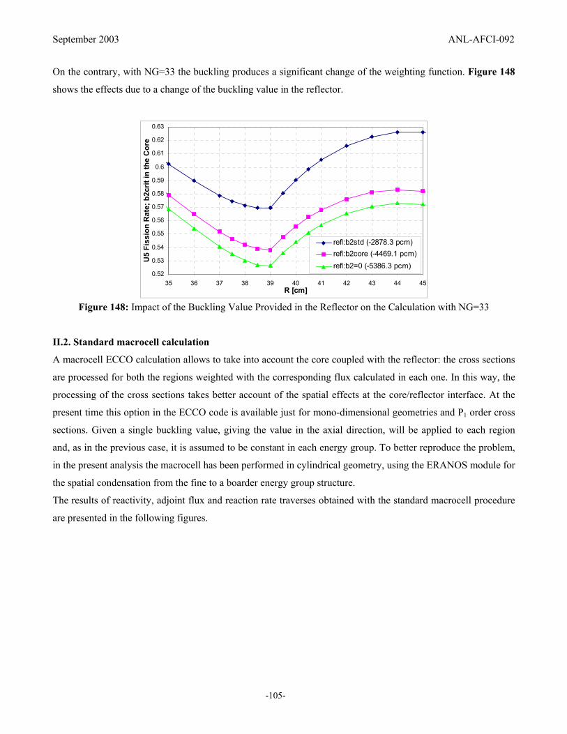
September 2003 ANL-AFCI-092
-105-
On the contrary, with NG=33 the buckling produces a significant change of the weighting function. Figure 148
shows the effects due to a change of the buckling value in the reflector.
0.52
0.53
0.54
0.55
0.56
0.57
0.58
0.59
0.6
0.61
0.62
0.63
35 36 37 38 39 40 41 42 43 44 45R [cm]
U5
Fiss
ion
Rat
e; b
2crit
in th
e C
ore
refl:b2std (-2878.3 pcm)refl:b2core (-4469.1 pcm)refl:b2=0 (-5386.3 pcm)
Figure 148: Impact of the Buckling Value Provided in the Reflector on the Calculation with NG=33
II.2. Standard macrocell calculation
A macrocell ECCO calculation allows to take into account the core coupled with the reflector: the cross sections
are processed for both the regions weighted with the corresponding flux calculated in each one. In this way, the
processing of the cross sections takes better account of the spatial effects at the core/reflector interface. At the
present time this option in the ECCO code is available just for mono-dimensional geometries and P1 order cross
sections. Given a single buckling value, giving the value in the axial direction, will be applied to each region
and, as in the previous case, it is assumed to be constant in each energy group. To better reproduce the problem,
in the present analysis the macrocell has been performed in cylindrical geometry, using the ERANOS module for
the spatial condensation from the fine to a boarder energy group structure.
The results of reactivity, adjoint flux and reaction rate traverses obtained with the standard macrocell procedure
are presented in the following figures.

September 2003 ANL-AFCI-092
-106-
0.54
0.55
0.56
0.57
0.58
0.59
0.6
0.61
0.62
0.63
0.64
35 36 37 38 39 40 41 42 43 44 45R [cm]
U5
Fiss
ion
Rat
e
1968gr; rho=-588.0 pcm838gr; rho=-799.8 pcm471gr; rho=-1131.4 pcm299gr; rho=-1485.9 pcm33gr; rho=-4154.6 pcm
Figure 149: U235 Fission Rate Distribution at the Interface
2.3
2.4
2.5
2.6
2.7
2.8
2.9
3
44 45 46 47 48 49 50 51 52 53 54R [cm]
U8
Cap
ture
Rat
e
1968gr; rho=-588.0 pcm838gr; rho=-799.8 pcm471gr; rho=-1131.4 pcm299gr; rho=-1485.9 pcm33gr; rho=-4154.6 pcm
Figure 150: U238 Capture Rate Distribution in the Reflector
0.5
0.52
0.54
0.56
0.58
0.6
0.62
0.64
0.66
35 36 37 38 39 40 41 42 43 44 45R [cm]
Pu9
Fiss
ion
Rat
e
1968gr; rho=-588.0 pcm838gr; rho=-799.8 pcm471gr; rho=-1131.4 pcm299gr; rho=-1485.9 pcm33gr; rho=-4154.6 pcm
Figure 151: Pu239 Fission Rate Distribution at the Interface

September 2003 ANL-AFCI-092
-107-
Also in the case of the standard macrocell a dependence of the results on the value chosen for the buckling has
been observed. In conclusion, this method doesn’t seem satisfactory because the 33-group calculation shows
huge discrepancies compared with the reference one. During this analysis, an inconsistency in the condensation
module of ERANOS was found: all the cross-sections to be weighted with the current (e.g. P1-total, transport
and all the cross-sections of order 1) are condensed with D*Φ, where D is the diffusion coefficient.
II.3. Improved macrocell calculation
Our investigation motivated the conception of a new macrocell, which makes properly use of the currents when
needed. The results are shown in the following figures and we can observe that the case with NG=33 reproduces
the reference calculation in a satisfactory manner both for the reactivity value and spatial distribution. The
results could be still improved if the reflector is divided into two regions (see Figures 152 to 154)
0.54
0.55
0.56
0.57
0.58
0.59
0.6
0.61
0.62
0.63
0.64
0.65
0.66
35 36 37 38 39 40 41 42 43 44 45R [cm]
U5
Fiss
ion
Rat
e
1968gr; rho=-588.0 pcm33gr std; rho=-4154.6 pcm33gr P1J; rho=-733.1 pcm33gr P1J (refl:5+35); rho=-262.3 pcm
Figure 152: U235 Fission Rate Distribution at the Interface
2.3
2.4
2.5
2.6
2.7
2.8
2.9
3
44 45 46 47 48 49 50 51 52 53 54R [cm]
U8
Cap
ture
Rat
e
1968gr; rho=-588.0 pcm33gr std; rho=-4154.6 pcm33gr P1J; rho=-733.1 pcm33gr P1J (refl:5+35); rho=-262.3 pcm
Figure 153: U238 Capture Rate Distribution in the Reflector
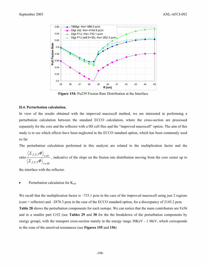
September 2003 ANL-AFCI-092
-108-
0.5
0.52
0.54
0.56
0.58
0.6
0.62
0.64
0.66
35 36 37 38 39 40 41 42 43 44 45R [cm]
Pu9
Fiss
ion
Rat
e
1968gr; rho=-588.0 pcm33gr std; rho=-4154.6 pcm33gr P1J; rho=-733.1 pcm33gr P1J (refl:5+35); rho=-262.3 pcm
Figure 154: Pu239 Fission Rate Distribution at the Interface
II.4. Perturbation calculation.
In view of the results obtained with the improved macrocell method, we are interested in performing a
perturbation calculation between the standard ECCO calculation, where the cross-section are processed
separately for the core and the reflector with a 0D cell flux and the “improved macrocell” option. The aim of this
study is to see which effects have been neglected in the ECCO standard option, which has been commonly used
so far.
The perturbation calculation performed in this analysis are related to the multiplication factor and the
ratio38r5U,f
0r5U,f
ΦΣ
ΦΣ
=
= , indicative of the slope on the fission rate distribution moving from the core center up to
the interface with the reflector.
• Perturbation calculation for Keff.
We recall that the multiplication factor is –733.1 pcm in the case of the improved macrocell using just 2 regions
(core + reflector) and –2878.3 pcm in the case of the ECCO standard option, for a discrepancy of 2145.2 pcm.
Table 28 shows the perturbation components for each isotope. We can notice that the main contributors are Fe56
and in a smaller part Cr52 (see Tables 29 and 30 for the the breakdown of the perturbation components by
energy group), with the transport cross-section mainly in the energy range 30KeV - 1 MeV, which corresponds
to the zone of the unsolved resonances (see Figures 155 and 156)

September 2003 ANL-AFCI-092
-109-
Table 28: Perturbation Calculation for Keff between Improved Macrocell and ECCO Standard
% Capture Fission Transport Elastic Inelastic N,XN SUM U238 -4.97 0.73 3.50 0.75 0.52 -0.01 0.52 Pu239 -4.84 6.24 4.23 -0.03 0.26 0.00 5.86 Fe56 -170.7 0.0 -1389.1 0.1 -3.9 0.1 -1563.7 Cr52 -16.5 0.0 -326.9 2.3 -0.6 0.0 -341.7 Na -3.4 0.0 2.4 -0.6 0.0 0.0 -1.6 O -1.1 0.0 1.9 1.8 0.0 0.0 2.6
Total -201.5 7.0 -1704.0 4.3 -3.7 0.1 -1898.0

September 2003 ANL-AFCI-092
-110-
Table 29: Fe56 Contribution in pcm
Gr. Energy [MeV] Capture Fission Transport Elastic Inelastic N,XN SUM 1 1.964E+1 0.0 0.0 0.0 0.0 0.0 0.1 0.1 2 1.000E+1 -0.2 0.0 -0.3 0.0 0.1 0.0 -0.4 3 6.065E+0 -0.2 0.0 -0.5 0.0 -0.1 0.0 -0.7 4 3.679E+0 0.0 0.0 -1.8 -0.9 -0.1 0.0 -2.8 5 2.231E+0 0.0 0.0 -5.7 0.5 0.1 0.0 -5.1 6 1.353E+0 0.0 0.0 -12.4 0.8 -4.0 0.0 -15.6 7 8.209E-1 -0.6 0.0 -79.5 1.0 0.0 0.0 -79.0 8 4.979E-1 -3.1 0.0 -166.9 -0.1 0.0 0.0 -170.0 9 3.020E-1 -2.2 0.0 -213.6 -8.2 0.0 0.0 -223.9 10 1.832E-1 -2.7 0.0 -192.8 -0.2 0.0 0.0 -195.7 11 1.111E-1 -8.8 0.0 -313.4 -3.5 0.0 0.0 -325.7 12 6.738E-2 0.3 0.0 8.1 -16.5 0.0 0.0 -8.1 13 4.087E-2 -5.2 0.0 -286.5 0.5 0.0 0.0 -291.2 14 2.479E-2 0.0 0.0 -127.1 36.1 0.0 0.0 -91.0 15 1.503E-2 0.0 0.0 1.8 -0.9 0.0 0.0 0.9 16 9.119E-3 0.0 0.0 0.4 -1.9 0.0 0.0 -1.6 17 5.531E-3 0.0 0.0 0.0 -0.4 0.0 0.0 -0.4 18 3.355E-3 0.0 0.0 0.0 0.0 0.0 0.0 0.0 19 2.035E-3 0.0 0.0 0.0 -0.2 0.0 0.0 -0.3 20 1.234E-3 -2.1 0.0 0.2 1.1 0.0 0.0 -0.9 21 7.485E-4 0.0 0.0 0.2 -1.6 0.0 0.0 -1.4 22 4.540E-4 0.0 0.0 0.0 -1.4 0.0 0.0 -1.3 23 3.043E-4 0.0 0.0 0.0 -2.3 0.0 0.0 -2.2 24 1.486E-4 0.0 0.0 0.0 -1.7 0.0 0.0 -1.7 25 9.166E-5 0.0 0.0 0.0 0.6 0.0 0.0 0.6 26 6.790E-5 0.0 0.0 0.0 1.1 0.0 0.0 1.1 27 4.017E-5 0.0 0.0 0.0 -1.0 0.0 0.0 -1.0 28 2.260E-5 0.0 0.0 0.0 -0.3 0.0 0.0 -0.3 29 1.371E-5 0.0 0.0 0.0 0.4 0.0 0.0 0.4 30 8.315E-6 0.0 0.0 0.0 -0.4 0.0 0.0 -0.4 31 4.000E-6 -135.0 0.0 0.5 -0.5 0.0 0.0 -135.0 32 5.400E-7 -10.9 0.0 0.0 0.0 0.0 0.0 -10.9 33 1.000E-7 -0.1 0.0 0.0 0.0 0.0 0.0 -0.1
SUM -170.7 0.0 -1389.1 0.1 -3.9 0.1 -1563.7
1 2 3 4 5 6 7 8 9 10 11 12 13 14 15 16 17 18 19 20 21 22 23 24 25 26 27 28 29 30 31 32 33
CAPTUREFISSION
TRANSPORTELAST_REMOVAL
INEL_REMOVALN,XN_REMOVAL
-0.05
0
0.05
0.1
0.15
0.2
0.25
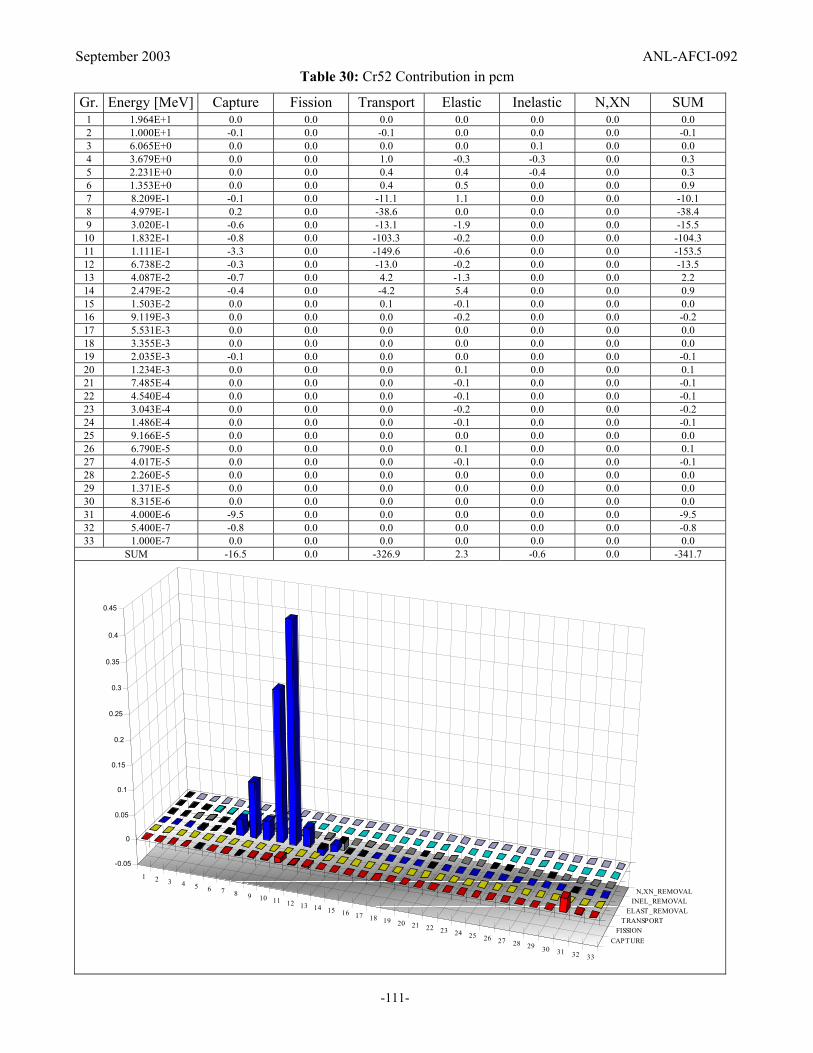
September 2003 ANL-AFCI-092
-111-
Table 30: Cr52 Contribution in pcm
Gr. Energy [MeV] Capture Fission Transport Elastic Inelastic N,XN SUM 1 1.964E+1 0.0 0.0 0.0 0.0 0.0 0.0 0.0 2 1.000E+1 -0.1 0.0 -0.1 0.0 0.0 0.0 -0.1 3 6.065E+0 0.0 0.0 0.0 0.0 0.1 0.0 0.0 4 3.679E+0 0.0 0.0 1.0 -0.3 -0.3 0.0 0.3 5 2.231E+0 0.0 0.0 0.4 0.4 -0.4 0.0 0.3 6 1.353E+0 0.0 0.0 0.4 0.5 0.0 0.0 0.9 7 8.209E-1 -0.1 0.0 -11.1 1.1 0.0 0.0 -10.1 8 4.979E-1 0.2 0.0 -38.6 0.0 0.0 0.0 -38.4 9 3.020E-1 -0.6 0.0 -13.1 -1.9 0.0 0.0 -15.5 10 1.832E-1 -0.8 0.0 -103.3 -0.2 0.0 0.0 -104.3 11 1.111E-1 -3.3 0.0 -149.6 -0.6 0.0 0.0 -153.5 12 6.738E-2 -0.3 0.0 -13.0 -0.2 0.0 0.0 -13.5 13 4.087E-2 -0.7 0.0 4.2 -1.3 0.0 0.0 2.2 14 2.479E-2 -0.4 0.0 -4.2 5.4 0.0 0.0 0.9 15 1.503E-2 0.0 0.0 0.1 -0.1 0.0 0.0 0.0 16 9.119E-3 0.0 0.0 0.0 -0.2 0.0 0.0 -0.2 17 5.531E-3 0.0 0.0 0.0 0.0 0.0 0.0 0.0 18 3.355E-3 0.0 0.0 0.0 0.0 0.0 0.0 0.0 19 2.035E-3 -0.1 0.0 0.0 0.0 0.0 0.0 -0.1 20 1.234E-3 0.0 0.0 0.0 0.1 0.0 0.0 0.1 21 7.485E-4 0.0 0.0 0.0 -0.1 0.0 0.0 -0.1 22 4.540E-4 0.0 0.0 0.0 -0.1 0.0 0.0 -0.1 23 3.043E-4 0.0 0.0 0.0 -0.2 0.0 0.0 -0.2 24 1.486E-4 0.0 0.0 0.0 -0.1 0.0 0.0 -0.1 25 9.166E-5 0.0 0.0 0.0 0.0 0.0 0.0 0.0 26 6.790E-5 0.0 0.0 0.0 0.1 0.0 0.0 0.1 27 4.017E-5 0.0 0.0 0.0 -0.1 0.0 0.0 -0.1 28 2.260E-5 0.0 0.0 0.0 0.0 0.0 0.0 0.0 29 1.371E-5 0.0 0.0 0.0 0.0 0.0 0.0 0.0 30 8.315E-6 0.0 0.0 0.0 0.0 0.0 0.0 0.0 31 4.000E-6 -9.5 0.0 0.0 0.0 0.0 0.0 -9.5 32 5.400E-7 -0.8 0.0 0.0 0.0 0.0 0.0 -0.8 33 1.000E-7 0.0 0.0 0.0 0.0 0.0 0.0 0.0
SUM -16.5 0.0 -326.9 2.3 -0.6 0.0 -341.7
1 2 3 4 5 6 7 8 9 10 11 12 13 14 15 16 17 18 19 20 21 22 23 24 25 26 27 28 29 30 31 32 33
CAPTUREFISSION
TRANSPORTELAST_REMOVAL
INEL_REMOVALN,XN_REMOVAL
-0.05
0
0.05
0.1
0.15
0.2
0.25
0.3
0.35
0.4
0.45

September 2003 ANL-AFCI-092
-112-
Fe56
1E-5
1E-4
1E-3
1E-2
1E-1
1E+0
1E+1
1E+2
1E-8 1E-7 1E-6 1E-5 1E-4 1E-3 1E-2 1E-1 1E+0 1E+1 1E+2Energy [MeV]
Bar
ns
ELASTIC
N,XN
INELASTICCAPTURE
Figure 155: Fe56 Cross-Sections
Cr52
1E-5
1E-4
1E-3
1E-2
1E-1
1E+0
1E+1
1E+2
1E-8 1E-7 1E-6 1E-5 1E-4 1E-3 1E-2 1E-1 1E+0 1E+1 1E+2Energy [MeV]
Bar
ns
ELASTIC
N,XN
INELASTICCAPTURE
Figure 156: Cr52 Cross-Sections
• Perturbation calculation for 38r5U,f
0r5U,f
ΦΣ
ΦΣ
=
=
As far as the ratio 38r5U,f
0r5U,f
ΦΣ
ΦΣ
=
= , the value is 4.42E-2 in the case of the improved macrocell and 4.66E-2 for
the ECCO standard option. The discrepancy is then: (ECCO standard – Improved macrocell)/Improved
macrocell = 5%. Table 31 shows the perturbation components for each isotope. We can notice that the main
contributors are again Fe56 and in a smaller part Cr52 (see Tables 32 and 33 for the the breakdown of the
perturbation components by energy group), with the transport and elastic cross-section once again mainly in the
energy range 30KeV - 1 MeV.
Table 31: Perturbation Calculation for 38r5U,f
0r5U,f
ΦΣ
ΦΣ
=
= between Improved Macrocell and ECCO Standard.
% Capture Fission Transport Elastic Inelastic N,XN SUM U238 0.38 0.00 -0.06 0.01 0.00 0.00 0.33 Pu239 0.04 0.21 0.10 0.00 0.00 0.00 0.35 Fe56 0.81 0.00 3.20 -0.78 0.00 0.00 3.23 Cr52 0.06 0.00 0.60 0.02 0.00 0.00 0.68 Na 0.02 0.00 -0.38 0.05 0.00 0.00 -0.31 O 0.00 0.00 -0.01 0.03 0.00 0.00 0.02
Total 1.31 0.21 3.45 -0.67 0.00 0.00 4.3

September 2003 ANL-AFCI-092
-113-
Table 32: Fe56 Contribution in %
Gr. Energy [MeV] Capture Fission Transport Elastic Inelastic N,XN SUM 1 1.964E+1 0.00 0.00 0.00 0.00 0.00 0.00 0.00 2 1.000E+1 0.00 0.00 0.00 0.00 0.00 0.00 0.00 3 6.065E+0 0.00 0.00 0.00 0.00 0.00 0.00 0.00 4 3.679E+0 0.00 0.00 0.00 0.00 0.00 0.00 0.00 5 2.231E+0 0.00 0.00 -0.01 0.00 0.00 0.00 -0.01 6 1.353E+0 0.00 0.00 0.00 -0.01 0.00 0.00 -0.01 7 8.209E-1 0.00 0.00 0.01 0.00 0.00 0.00 0.01 8 4.979E-1 0.00 0.00 0.19 0.12 0.00 0.00 0.31 9 3.020E-1 0.00 0.00 0.23 -0.12 0.00 0.00 0.11 10 1.832E-1 0.00 0.00 0.37 0.00 0.00 0.00 0.36 11 1.111E-1 0.01 0.00 0.71 0.10 0.00 0.00 0.82 12 6.738E-2 0.00 0.00 -0.02 -0.13 0.00 0.00 -0.16 13 4.087E-2 0.01 0.00 1.30 -0.02 0.00 0.00 1.29 14 2.479E-2 0.00 0.00 0.44 -0.49 0.00 0.00 -0.06 15 1.503E-2 0.00 0.00 -0.01 -0.14 0.00 0.00 -0.15 16 9.119E-3 0.00 0.00 -0.01 -0.05 0.00 0.00 -0.05 17 5.531E-3 0.00 0.00 0.00 0.00 0.00 0.00 -0.01 18 3.355E-3 0.00 0.00 0.00 0.00 0.00 0.00 0.00 19 2.035E-3 0.00 0.00 0.00 -0.02 0.00 0.00 -0.02 20 1.234E-3 -0.04 0.00 0.01 -0.04 0.00 0.00 -0.07 21 7.485E-4 0.00 0.00 0.01 0.00 0.00 0.00 0.01 22 4.540E-4 0.00 0.00 0.00 0.00 0.00 0.00 0.00 23 3.043E-4 0.00 0.00 0.00 0.00 0.00 0.00 0.00 24 1.486E-4 0.00 0.00 0.00 0.00 0.00 0.00 0.00 25 9.166E-5 0.00 0.00 0.00 0.01 0.00 0.00 0.01 26 6.790E-5 0.00 0.00 0.00 0.02 0.00 0.00 0.02 27 4.017E-5 0.00 0.00 0.00 -0.01 0.00 0.00 -0.01 28 2.260E-5 0.00 0.00 0.00 0.01 0.00 0.00 0.01 29 1.371E-5 0.00 0.00 0.00 -0.02 0.00 0.00 -0.02 30 8.315E-6 0.00 0.00 0.00 0.00 0.00 0.00 0.00 31 4.000E-6 0.81 0.00 0.00 0.01 0.00 0.00 0.82 32 5.400E-7 0.01 0.00 0.00 0.00 0.00 0.00 0.01 33 1.000E-7 0.00 0.00 0.00 0.00 0.00 0.00 0.00
SUM 0.81 0.00 3.20 -0.78 0.00 0.00 3.23
1 2 3 4 5 6 7 8 9 10 11 12 13 14 15 16 17 18 19 20 21 22 23 24 25 26 27 28 29 30 31 32 33
CAPTUREFISSION
TRANSPORTELAST_REMOVAL
INEL_REMOVALN,XN_REMOVAL
-0.15
-0.05
0.05
0.15
0.25
0.35
0.45

September 2003 ANL-AFCI-092
-114-
Table 33: Cr52 Contribution in %
Gr. Energy [MeV] Capture Fission Transport Elastic Inelastic N,XN SUM 1 1.964E+1 0.00 0.00 0.00 0.00 0.00 0.00 0.00 2 1.000E+1 0.00 0.00 0.00 0.00 0.00 0.00 0.00 3 6.065E+0 0.00 0.00 0.00 0.00 0.00 0.00 0.00 4 3.679E+0 0.00 0.00 0.00 0.00 0.00 0.00 0.00 5 2.231E+0 0.00 0.00 0.00 0.00 0.00 0.00 0.00 6 1.353E+0 0.00 0.00 0.00 -0.01 0.00 0.00 -0.01 7 8.209E-1 0.00 0.00 0.00 0.00 0.00 0.00 0.00 8 4.979E-1 0.00 0.00 0.03 0.08 0.00 0.00 0.11 9 3.020E-1 0.00 0.00 0.01 -0.03 0.00 0.00 -0.02 10 1.832E-1 0.00 0.00 0.16 0.00 0.00 0.00 0.16 11 1.111E-1 0.00 0.00 0.34 0.02 0.00 0.00 0.36 12 6.738E-2 0.00 0.00 0.06 0.00 0.00 0.00 0.06 13 4.087E-2 0.00 0.00 -0.01 0.06 0.00 0.00 0.05 14 2.479E-2 0.00 0.00 0.01 -0.07 0.00 0.00 -0.06 15 1.503E-2 0.00 0.00 0.00 -0.02 0.00 0.00 -0.02 16 9.119E-3 0.00 0.00 0.00 -0.01 0.00 0.00 -0.01 17 5.531E-3 0.00 0.00 0.00 0.00 0.00 0.00 0.00 18 3.355E-3 0.00 0.00 0.00 0.00 0.00 0.00 0.00 19 2.035E-3 0.00 0.00 0.00 0.00 0.00 0.00 0.00 20 1.234E-3 0.00 0.00 0.00 0.00 0.00 0.00 0.00 21 7.485E-4 0.00 0.00 0.00 0.00 0.00 0.00 0.00 22 4.540E-4 0.00 0.00 0.00 0.00 0.00 0.00 0.00 23 3.043E-4 0.00 0.00 0.00 0.00 0.00 0.00 0.00 24 1.486E-4 0.00 0.00 0.00 0.00 0.00 0.00 0.00 25 9.166E-5 0.00 0.00 0.00 0.00 0.00 0.00 0.00 26 6.790E-5 0.00 0.00 0.00 0.00 0.00 0.00 0.00 27 4.017E-5 0.00 0.00 0.00 0.00 0.00 0.00 0.00 28 2.260E-5 0.00 0.00 0.00 0.00 0.00 0.00 0.00 29 1.371E-5 0.00 0.00 0.00 0.00 0.00 0.00 0.00 30 8.315E-6 0.00 0.00 0.00 0.00 0.00 0.00 0.00 31 4.000E-6 0.06 0.00 0.00 0.00 0.00 0.00 0.06 32 5.400E-7 0.00 0.00 0.00 0.00 0.00 0.00 0.00 33 1.000E-7 0.00 0.00 0.00 0.00 0.00 0.00 0.00
SUM 0.06 0.00 0.60 0.02 0.00 0.00 0.68
1 2 3 4 5 6 7 8 9 10 11 12 13 14 15 16 17 18 19 20 21 22 23 24 25 26 27 28 29 30 31 32 33
CAPTUREFISSION
TRANSPORTELAST_REMOVAL
INEL_REMOVALN,XN_REMOVAL
-0.15
-0.05
0.05
0.15
0.25
0.35
0.45

September 2003 ANL-AFCI-092
-115-
II.5. Application of the improved macrocell option to a 2D model.
After an extensive study of the effects located at the interface core/reflector for a simple 1D model, we want to
complete our analysis by an application to a more realistic model in RZ geometry. The effort performed at this
point will also represents the base for the development of a standard procedure for the treatment of the
core/reflector interface effects in a general 3D geometry.
Two RZ models have been object of our study. Table 34 shows geometry and composition of the first system. A
second model, which will be investigate later in this document, has been obtained by reducing the height of the
core zone in order to strengthen the fraction of neutrons escaping from the core in the reflector and produce
situation with high effects at the interface.
Table 34: Geometry and Isotopic Compositions for a 2D Model
Region Isotope Density × 10+24 at/cm3
Pu239 1.5×10⁻³
U238 5.0×10⁻³
Fe56 7.0×10⁻³
Cr52 1.5×10⁻³
Na23 1.0×10⁻²
Zone1- Core
O16 1.5×10⁻²
Fe56 5.0×10⁻²
Cr52 1.5×10⁻²
Zone2 - Reflector
Na23 5.0×10⁻³
Figures 157 to 159 show the radial traverses, calculated at Z=103 cm and normalized to 1 at the core center
(R=0);
Figures 160 to 162 show the axial traverses, calculated along the radial position R=10 cm and normalized to 1 at
Z=97 cm.
These traverses have been obtained using cross-sections obtained in the standard way (ECCO standard option)
and the case with NG=1968 is always considered as the reference case. An expanded viewat the interface is
performed in order to stress the effects on the distribution and the reactivity through NG.
We can notice that the effects on the reactivity are very huge: about 4000 pcm moving from NG=33 to
NG=1968. With NG=471 we still have 600 pcm of discrepancy compared with the reference.
The reactivity value calculated with JEF2.2/MCNP4C is –109 ± 13 pcm, which is in good agreement with the
fine calculation.

September 2003 ANL-AFCI-092
-116-
Referring to the reaction rate distributions, both axial and radial traverses exhibit a similar behavior: the case
with NG=299 can be already considered as representative of the reference calculation in this case.
Note that, because of the high computational resources (memory and disk space) required by the fine calculation
(NG=1968) just in this case a spatial grid a little bit boarder has been used. Within a distance of 5 cm from the
interface both in the core and in the reflector side the same grid as in the other calculations with lower NG has
been kept. The grid effects both on reactivity and on spatial distributions have been investigated and they were
found to be negligible.
0.54
0.55
0.56
0.57
0.58
0.59
0.6
0.61
0.62
0.63
0.64
35 36 37 38 39 40 41 42 43 44 45R [cm]
U5
Fiss
ion
Rat
e
1968gr; rho=73.1 pcm838gr; rho=-170.3 pcm471gr; rho=-537.4 pcm299gr; rho=-924.4 pcm33gr; rho=-3886.4 pcm
Figure 157: U235 Fission Rate Radial (Z=103 cm) Traverse at the Interface
2.2
2.3
2.4
2.5
2.6
2.7
2.8
2.9
3
44 45 46 47 48 49 50 51 52 53 54R [cm]
U8
Cap
ture
Rat
e
1968gr; rho=73.1 pcm838gr; rho=-170.3 pcm471gr; rho=-537.4 pcm299gr; rho=-924.4 pcm33gr; rho=-3886.4 pcm
Figure 158: U238 Capture Rate Radial (Z=103 cm) Traverse in the Reflector
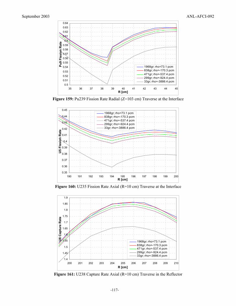
September 2003 ANL-AFCI-092
-117-
0.50.510.520.53
0.540.550.560.570.580.590.6
0.610.620.630.64
35 36 37 38 39 40 41 42 43 44 45R [cm]
Pu9
Fiss
ion
Rat
e
1968gr; rho=73.1 pcm838gr; rho=-170.3 pcm471gr; rho=-537.4 pcm299gr; rho=-924.4 pcm33gr; rho=-3886.4 pcm
Figure 159: Pu239 Fission Rate Radial (Z=103 cm) Traverse at the Interface
0.35
0.36
0.37
0.38
0.39
0.4
0.41
0.42
0.43
0.44
0.45
190 191 192 193 194 195 196 197 198 199 200R [cm]
U5
Fiss
ion
Rat
e
1968gr; rho=73.1 pcm838gr; rho=-170.3 pcm471gr; rho=-537.4 pcm299gr; rho=-924.4 pcm33gr; rho=-3886.4 pcm
Figure 160: U235 Fission Rate Axial (R=10 cm) Traverse at the Interface
1.4
1.45
1.5
1.55
1.6
1.65
1.7
1.75
1.8
1.85
1.9
200 201 202 203 204 205 206 207 208 209 210R [cm]
U8
Cap
ture
Rat
e
1968gr; rho=73.1 pcm838gr; rho=-170.3 pcm471gr; rho=-537.4 pcm299gr; rho=-924.4 pcm33gr; rho=-3886.4 pcm
Figure 161: U238 Capture Rate Axial (R=10 cm) Traverse in the Reflector

September 2003 ANL-AFCI-092
-118-
0.32
0.33
0.34
0.35
0.36
0.37
0.38
0.39
0.4
0.41
0.42
0.43
190 191 192 193 194 195 196 197 198 199 200R [cm]
Pu9
Fiss
ion
Rat
e
1968gr; rho=73.1 pcm838gr; rho=-170.3 pcm471gr; rho=-537.4 pcm299gr; rho=-924.4 pcm33gr; rho=-3886.4 pcm
Figure 162: Pu239 Fission Rate Axial (R=10 cm) Traverse at the Interface
So far we investigated the impact through NG in term of reactivity and reaction rate traverses of the system
under study. Our goal at this point is to find a method to process the cross-sections with low NG (in particular
with NG=33 to be consistent with the energy group structure usually adopted) able to reproduce approximately
the same results provided by the fine calculation (NG=1968). In this attempt, we consider our objective reached
if the new cross-sections recover 90% of discrepancy observed on the reactivity and reduce the discrepancies on
the traverses to about 2%.
For this purpose, the following procedure has been used. A 1D model has been drawn from the radial direction
of the 2D problem as shown in Figure 163. In the flux calculation we provided an axial buckling, determined in
order to give with NG=1968 the same multiplication factor of the corresponding 2D calculation. In order to
satisfy this requirement, the buckling has been calculated to be of a value of 2.6E-4. In fact, using the formula
for cylindrical coordinates: B2ax=(π/H)2 we derive H=194.8 cm with an extrapolated distance of 20.41 cm. Table
35 shows that the reactivity change through NG for the 1D model so defined reproduce approximately the same
variation of the original 2D system.

September 2003 ANL-AFCI-092
-119-
Figure 163: 1D Geometry for Cross-Sections Condensation
Table 35: Reactivity Value for 1D and 2D Models
NG 1D model with B2ax=2.6E-4 2D Model
33 -3741.3 pcm -3886.4 pcm 299 -1070.2 pcm -924.4 pcm 471 -714.3 pcm -537.4 pcm 838 -383.3 pcm -170.3 pcm
1968 -171.2 pcm 73.1 pcm
Once fixed the 1D model, according to the improved macrocell scheme we chose to collapse the cross-sections
from NG=1968 to NG=33 using as weighting function the flux and the currents solution of this 1D model. The
cross-sections so obtained are then used in the original 2D system and the results are reported in the following
figures. In particular the case with the reflector divided into two regions appears to be very satisfactory: in the
comparison NG=1968 vs NG=33 the discrepancy on the reactivity is reduced from 4000 to 150 pcm and the
traverses both radial and axial agree within a margin less than 1%.
0.53
0.54
0.55
0.56
0.57
0.58
0.59
0.6
0.61
0.62
0.63
0.64
0.65
0.66
35 36 37 38 39 40 41 42 43 44 45R [cm]
U5
Fiss
ion
Rat
e
1968gr; rho=73.1 pcm33gr std; rho=-3886.4 pcm33gr P1J; rho=-245.2 pcm33gr P1J (refl: 5+25); rho=230.7 pcm
Figure 164: U235 Fission Rate Radial (Z=103 cm) Traverse at the Interface Using the Improved Macrocell Scheme
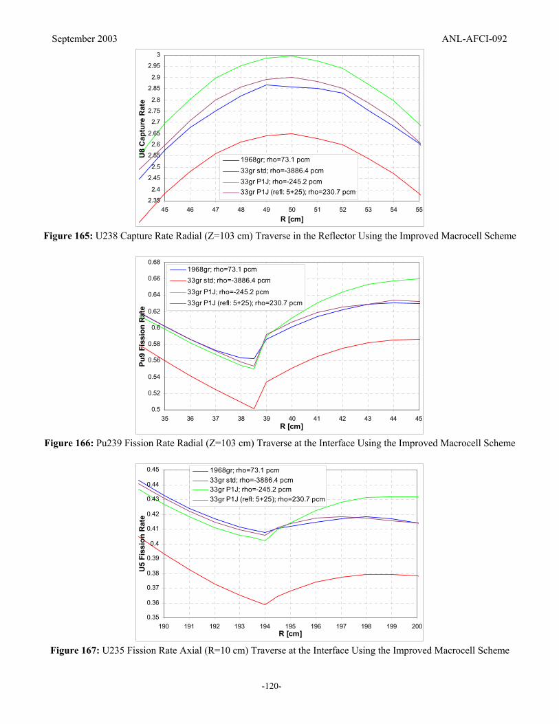
September 2003 ANL-AFCI-092
-120-
2.35
2.4
2.45
2.5
2.55
2.6
2.65
2.7
2.75
2.8
2.85
2.9
2.95
3
45 46 47 48 49 50 51 52 53 54 55R [cm]
U8
Cap
ture
Rat
e
1968gr; rho=73.1 pcm33gr std; rho=-3886.4 pcm33gr P1J; rho=-245.2 pcm33gr P1J (refl: 5+25); rho=230.7 pcm
Figure 165: U238 Capture Rate Radial (Z=103 cm) Traverse in the Reflector Using the Improved Macrocell Scheme
0.5
0.52
0.54
0.56
0.58
0.6
0.62
0.64
0.66
0.68
35 36 37 38 39 40 41 42 43 44 45R [cm]
Pu9
Fiss
ion
Rat
e
1968gr; rho=73.1 pcm33gr std; rho=-3886.4 pcm
33gr P1J; rho=-245.2 pcm33gr P1J (refl: 5+25); rho=230.7 pcm
Figure 166: Pu239 Fission Rate Radial (Z=103 cm) Traverse at the Interface Using the Improved Macrocell Scheme
0.35
0.36
0.37
0.38
0.39
0.4
0.41
0.42
0.43
0.44
0.45
190 191 192 193 194 195 196 197 198 199 200R [cm]
U5
Fiss
ion
Rat
e
1968gr; rho=73.1 pcm33gr std; rho=-3886.4 pcm33gr P1J; rho=-245.2 pcm33gr P1J (refl: 5+25); rho=230.7 pcm
Figure 167: U235 Fission Rate Axial (R=10 cm) Traverse at the Interface Using the Improved Macrocell Scheme

September 2003 ANL-AFCI-092
-121-
1.4
1.45
1.5
1.55
1.6
1.65
1.7
1.75
1.8
1.85
1.9
1.95
2
200 201 202 203 204 205 206 207 208 209 210R [cm]
U8
Cap
ture
Rat
e
1968gr; rho=73.1 pcm33gr std; rho=-3886.4 pcm33gr P1J; rho=-245.2 pcm33gr P1J (refl: 5+25); rho=230.7 pcm
Figure 168: U238 Capture Rate Axial (R=10 cm) Traverse in the Reflector Using the Improved Macrocell Scheme
0.32
0.34
0.36
0.38
0.4
0.42
0.44
190 191 192 193 194 195 196 197 198 199 200R [cm]
Pu9
Fiss
ion
Rat
e
1968gr; rho=73.1 pcm33gr std; rho=-3886.4 pcm33gr P1J; rho=-245.2 pcm33gr P1J (refl: 5+25); rho=230.7 pcm
Figure 169: Pu239 Fission Rate Axial (R=10 cm) Traverse at the Interface Using the Improved Macrocell Scheme
As anticipated, we want to investigate also a second model with smaller height of the core zone, in order to
strengthen the fraction of neutrons escaping from the core in the reflector and produce situation with high effects
at the interface.
Table 36 shows geometry and composition of the new 2D model.

September 2003 ANL-AFCI-092
-122-
Table 36: Geometry and Isotopic Compositions for a 2D Model
Region Isotope Density × 10+24 at/cm3
Pu239 1.88×10⁻³
U238 6.25×10⁻³
Fe56 7.0×10⁻³
Cr52 1.5×10⁻³
Na23 1.0×10⁻²
Zone1- Core
O16 1.5×10⁻²
Fe56 5.0×10⁻²
Cr52 1.5×10⁻²
Zone2 - Reflector
Na23 5.0×10⁻³
As in the previous example, the following figures report reactivity and traverses calculated in the standard way.
The reactivity value calculated with JEF2.2/MCNP4C is –31 ± 13 pcm, which is in good agreement with the fine
calculation.
Again, the radial traverses (see Figures 170 to 172) are normalized to 1 at the core center (R=0) and the axial
ones (see Figures 173 to 175) at Z=59 cm.
0.45
0.46
0.47
0.48
0.49
0.5
0.51
0.52
0.53
0.54
0.55
0.56
0.57
0.58
35 36 37 38 39 40 41 42 43 44 45R [cm]
U5
Fiss
ion
Rat
e
1968gr; rho=94.2 pcm838gr; rho=-126.8 pcm471gr; rho=-488.7 pcm299gr; rho=-857.7 pcm33gr; rho=-3709.0 pcm
Figure 170: U235 Fission Rate Radial (Z=65 cm) Traverse at the Interface

September 2003 ANL-AFCI-092
-123-
1.7
1.75
1.8
1.85
1.9
1.95
2
2.05
2.1
2.15
2.2
44 45 46 47 48 49 50 51 52 53 54R [cm]
U8
Cap
ture
Rat
e
1968gr; rho=94.2 pcm838gr; rho=-126.8 pcm471gr; rho=-488.7 pcm299gr; rho=-857.7 pcm33gr; rho=-3709.0 pcm
Figure 171: U238 Capture Rate Radial (Z=65 cm) Traverse in the Reflector
0.43
0.44
0.45
0.46
0.47
0.48
0.49
0.5
0.51
0.52
0.53
0.54
0.55
35 36 37 38 39 40 41 42 43 44 45R [cm]
Pu9
Fiss
ion
Rat
e
1968gr; rho=94.2 pcm838gr; rho=-126.8 pcm471gr; rho=-488.7 pcm299gr; rho=-857.7 pcm33gr; rho=-3709.0 pcm
Figure 172: Pu239 Fission Rate Radial (Z=65 cm) Traverse at the Interface
0.52
0.54
0.56
0.58
0.6
0.62
0.64
0.66
100 101 102 103 104 105 106 107 108 109 110R [cm]
U5
Fiss
ion
Rat
e
1968gr; rho=94.2 pcm838gr; rho=-126.8 pcm471gr; rho=-488.7 pcm299gr; rho=-857.7 pcm33gr; rho=-3709.0 pcm
Figure 173: U235 Fission Rate Axial (R=10 cm) Traverse at the Interface

September 2003 ANL-AFCI-092
-124-
1.9
2
2.1
2.2
2.3
2.4
2.5
2.6
110 111 112 113 114 115 116 117 118 119 120R [cm]
U8
Cap
ture
Rat
e
1968gr; rho=94.2 pcm838gr; rho=-126.8 pcm471gr; rho=-488.7 pcm299gr; rho=-857.7 pcm33gr; rho=-3709.0 pcm
Figure 174: U238 Capture Rate Axial (R=10 cm) Traverse in the Reflector
0.48
0.5
0.52
0.54
0.56
0.58
0.6
0.62
0.64
100 101 102 103 104 105 106 107 108 109 110R [cm]
Pu9
Fiss
ion
Rat
e
1968gr; rho=94.2 pcm838gr; rho=-126.8 pcm471gr; rho=-488.7 pcm299gr; rho=-857.7 pcm33gr; rho=-3709.0 pcm
Figure 175: Pu239 Fission Rate Axial (R=10 cm) Traverse at the Interface
In order to process the 33-group cross-sections able to reproduce approximately the same results provided by the
fine calculation (NG=1968) the same procedure as in the previous case has been used. The 1D model has been
drawn from the radial direction of the 2D problem is again as shown in Figure 163 and the axial buckling has
been evaluated to be of a value of 7.8E-4, corresponding to H=112.5 cm with an extrapolated distance of 19.3
cm. Table 37 shows the reactivity values for the 1D and the original 2D model.
Table 37: Reactivity Value for 1D and 2D Models
NG 1D model with B2ax =7.8E-4 2D Model
33 -2443.4 pcm -3709.0 pcm 299 -517.1 pcm -857.7 pcm 471 -257.8 pcm -488.7 pcm 838 -11.1 pcm -126.8 pcm
1968 138.9 pcm 94.2 pcm

September 2003 ANL-AFCI-092
-125-
Because of the high interface core/reflector effects, this time the improved macrocell gives good results if both
the core and the reflector are splitted into two regions.
In the following figures, we observe that the calculation labelled “33gr P1J”, corresponding to the case of a
macrocell with a single region for reflector and core, recovers just 200 pcm of the 3800 pcm of reactivity
discrepancy observed between the 33-group standard and the reference calculation. Splitting the reflector into
two regions (case “33gr P1J (refl:8+22)”) about 1100 pcm of this discrepancy is recovered. Just by splitting the
core into two regions (case “33gr P1J (core:9+31)”) an important gain is obtained. If the reflector is splitted into
two regions also the discrepancy on the rate distributions is dramatically reduced. The results so obtained are
satisfactory for us, because the 33-group calculation reproduce the reference one within the margin of
discrepancy requested both on reactivity value and fission rate (or flux) distribution.
Anyway, the final results we obtained could be still improved if a different size for the sub-regions in the core
and in the reflector is chosen. A similar choice has not yet been possible because in the current procedure the
total cross-section is current-weighted. Consequently, it happens that the condensation with the current given by
small sub-regions (5 cm e.g.), introduce negative values in few groups of the total cross-sections with
consequent error found by the code. A better solution could be represented by using a flux-weighted cross-
section, but at the moment this application is of a smaller interest.
Finally, for better results we could also split the core and the reflector into more than two regions. We want to
avoid this option, because is less practicable in the case of a general geometry in 3 dimensions. Indeed, our study
demonstrated that the procedure adopted for this 2D model will be certainly successful also in the case of more
complicated geometry, provided that the radial and axial reflector are made of the same material.
At this stage, any information cannot be provided for cases where radial and axial reflectors are made of
different materials. It could be possible that the more appropriate solution for this kind of problem is a 2D
macrocell.

September 2003 ANL-AFCI-092
-126-
0.45
0.47
0.49
0.51
0.53
0.55
0.57
0.59
0.61
35 36 37 38 39 40 41 42 43 44 45R [cm]
U5
Fiss
ion
Rat
e
1968gr; rho=94.2 pcm33gr std; rho=-3709.0 pcm33gr P1J; rho=-3489.0 pcm33gr P1J (refl: 8+22); rho=-2671.8 pcm33gr P1J (core: 9+31); rho=-0.9 pcm33gr P1J (core: 9+31; ref l: 6+24); rho=457.7 pcm
Figure 176: U235 Fission Rate Radial (Z=65 cm) Traverse at the Interface Using the Improved Macrocell Scheme
1.8
1.85
1.9
1.95
2
2.05
2.1
2.15
2.2
2.25
2.3
2.35
2.4
45 46 47 48 49 50 51 52 53 54 55R [cm]
U8
Cap
ture
Rat
e
1968gr; rho=94.2 pcm33gr std; rho=-3709.0 pcm33gr P1J; rho=-3489.0 pcm33gr P1J (refl: 8+22); rho=-2671.8 pcm33gr P1J (core: 9+31); rho=-0.9 pcm33gr P1J (core: 9+31; ref l: 6+24); rho=457.7 pcm
Figure 177: U238 Capture Rate Radial (Z=65 cm) Traverse in the Reflector Using the Improved Macrocell Scheme
0.43
0.44
0.45
0.46
0.47
0.48
0.49
0.5
0.51
0.52
0.53
0.54
0.55
0.56
35 36 37 38 39 40 41 42 43 44 45R [cm]
Pu9
Fiss
ion
Rat
e
1968gr; rho=94.2 pcm33gr std; rho=-3709.0 pcm33gr P1J; rho=-3489.0 pcm33gr P1J (ref l: 8+22); rho=-2671.8 pcm33gr P1J (core: 9+31); rho=-0.9 pcm33gr P1J (core: 9+31; refl: 6+24); rho=457.7 pcm
Figure 178: Pu239 Fission Rate Radial (Z=65 cm) Traverse at the Interface Using the Improved Macrocell Scheme

September 2003 ANL-AFCI-092
-127-
0.52
0.54
0.56
0.58
0.6
0.62
0.64
0.66
100 101 102 103 104 105 106 107 108 109 110R [cm]
U5
Fiss
ion
Rat
e
1968gr; rho=94.2 pcm33gr std; rho=-3709.0 pcm33gr P1J; rho=-3489.0 pcm33gr P1J (refl: 8+22); rho=-2671.8 pcm33gr P1J (core: 9+31); rho=-0.9 pcm33gr P1J (core: 9+31; refl: 6+24); rho=457.7 pcm
Figure 179: U235 Fission Rate Axial (R=10 cm) Traverse at the Interface Using the Improved Macrocell Scheme
1.9
2
2.1
2.2
2.3
2.4
2.5
2.6
2.7
110 111 112 113 114 115 116 117 118 119 120R [cm]
U8
Cap
ture
Rat
e
1968gr; rho=94.2 pcm33gr std; rho=-3709.0 pcm33gr P1J; rho=-3489.0 pcm33gr P1J (ref l: 8+22); rho=-2671.8 pcm33gr P1J (core: 9+31); rho=-0.9 pcm33gr P1J (core: 9+31; refl: 6+24); rho=457.7 pcm
Figure 180: U238 Capture Rate Axial (R=10 cm) Traverse in the Reflector Using the Improved Macrocell Scheme
0.48
0.5
0.52
0.54
0.56
0.58
0.6
0.62
0.64
100 101 102 103 104 105 106 107 108 109 110R [cm]
Pu9
Fiss
ion
Rat
e
1968gr; rho=94.2 pcm33gr std; rho=-3709.0 pcm33gr P1J; rho=-3489.0 pcm33gr P1J (refl: 8+22); rho=-2671.8 pcm33gr P1J (core: 9+31); rho=-0.9 pcm33gr P1J (core: 9+31; ref l: 6+24); rho=457.7 pcm
Figure 181: Pu239 Fission Rate Axial (R=10 cm) Traverse at the Interface Using the Improved Macrocell Scheme
September 2003 ANL-AFCI-092
-128-
References
[1] M. SALVATORES,
“Accelerator Driven System (ADS), Physics Principles and Specifities”,
J. Phys. IV France 9, pp. 7-17; 7-33, 1999
[2] M. DELPECH et al.,
“The Am and Cm Transmutation”,
Int. Conf. Global99 on Physics and Feasibility, Jackson, Wyoming – USA, August 29 – September 3,
1999
[3] M. SALVATORES, M. MARTINI, I. SLESSAREV,
“MUSE1: a First Experiment at MASURCA to Validate the Physics of Subcritical Multiplying Systems
Relevant to ADS”,
International Conference, Kalmar, Sweden, June 3-7, 1996
[4] R. SOULE, M. SALVATORES, R. JACQMIN,
“Validation of Neutronic Methods Applied to the Analysis of Fast Subcritical Systems: the MUSE2
Experiment”,
International Conference Global'97, Yokohama, Japan, October 5-10, 1997
[5] J.F. LEBRAT, R. SOULE, M. MARTINI, C.A. BOMPAS, P. BERTRAND, P. CHAUSSONNET, J.P.
CHAUVIN, M. SALVATORES , G. ALIBERTI, G. RIMPAULT,
“Experimental Investigation of Multiplying Subcritical Media in Presence of an External Source
Operating in Pulsed or Continuos Mode: the MUSE3 Experiment”,
International Conference, Prague, Czech Rep., 1999
[6] G. ALIBERTI, G. RIMPAULT, R. JACQMIN, J.F. LEBRAT, R. SOULE, J.P. CHAUVIN , G.
GRANGET, M. SALVATORES,
“Analysis of the MUSE-3 Subcritical Experiment”,
Int. Conf. Global2001, France, Paris, September 2001
[7] J.F. LEBRAT, R. SOULE, M. MARTINI, G. ALIBERTI, G. RIMPAULT, C.A. BOMPAS, P.
BERTRAND, P. CHAUSSONNET, J.P. CHAUVIN, M. SALVATORES,
“Experimental Investigation of Multiplying Subcritical Media Coupled with an Accelerator: the MUSE
Experiment”,

September 2003 ANL-AFCI-092
-129-
International Conference, Icenes, Portugal, October 5-10, 1997
[8] R. SOULE, W. ASSAL. D. VILLAMARIN
“Geometrical and Physical Data Associated to the MUSE4 ReferenceCconfiguration”,
CEA – Cadarache internal report
[9] J.VOLLAIRE, A. BILLEBAUD, R. BRISSOT. C. LE BRUN, E, LIATARD,
“Calibration and Monitoring of the GENEPI Neutron Source for the MUSE IV Experiment”,
LPSC, IN2P3-CNRS/UJF/INPG, 6 June 2003
[10] D. VILLAMARIN, R. SOULE, E. GONZALEZ,
“Benchmark on Computer Simulation of MASURCA Critical and Subcritical Experiments (MUSE-4
Benchmark)”,
NEA/SEN/NSC/WPPT(2001)5
[11] C. JAMMES, G. PERRET, G. IMEL,
“First MUSE-4 Experimental Results Based on Time Series Analysis”,
PHYSOR 2002, International Conference on the New Frontiers of Nuclear Technology : Reactor Physics,
Safety and High-performance Computing, Seoul, Korea, October 7-10, 2002
[12] G. ALIBERTI, G. PALMIOTTI, G. IMEL, C.G. STENBERG., R. BLOMQUIST, J. LIAW, P.J. FINCK,
“Analysis of the Experimental Measurements on the MUSE-4 Critical Configuration, Experimental
Results Based on Time Series Analysis and MUSE-4 Benchmark on Computer Simulation of
MASURCA”,
ANL-DOE Annual Report, September 2002.
[13] M. PLASCHY, C.A. BOMPAS, G. RIMPAULT,
“Paramètres de sûreté de l'expérience MUSE-4”,
CEA-Cadarache internal report (NT /DEN/SPRC/LEPH/99/231).
[14] “The Muse experiment for subcritical Neutronics Validation”,
CEA-Cadarache internal report.
[15] J.VOLLAIRE, A. BILLEBAUD, R. BRISSOT. C. LE BRUN, E, LIATARD,
“Calibration and Monitoring of the GENEPI Neutron Source for the MUSE IV Experiment ”,
Internal report (LPSC, IN2P3-CNRS/UJF/INPG, 6 June 2003).

September 2003 ANL-AFCI-092
-130-
[16] W ASSAL,
“Geometrical and Physical Description of the MASURCA Instrumental Assemblies Used for the βeff
Measurements During the MUSE-4 Experiments”,
CEA-Cadarache internal report (NT SPEx/LPE/03/046).
[17] R. SOULE, W ASSAL, D. VILLAMARIN,
“Geometrical and Physical Data Associated to the MUSE-4 Reference Configuration”,
CEA-Cadarache internal report (NT SPEx/LPE/01/015 December 21, 2001).
[18] R. SOULE, W ASSAL,
“Geometrical and Physical Description of the MASURCA Pilot Rod during the MUSE-4 Experiment”,
CEA-Cadarache internal report (NT SPEx/LPE/02/053 July 9, 2002).
[19] R. SOULE, W ASSAL,
“Geometrical and Physical Description of the Instrumental Assemblies Used by the CNRS/ISN during the
MUSE-4 Experiments”,
CEA-Cadarache internal report (NT SPEx/LPE/02/067 November 11, 2002).
[20] W ASSAL,
“Geometrical and Physical Description of the MASURCA Safety Rods during the MUSE-4 Experiments”,
CEA-Cadarache internal report (NT SPEx/LPE/02/063 March 7, 2003).
[21] M. THOMAS, C. JAMMES,
“Preliminary Numerical Estimation of Physical Quantities for Reference Core MUSE-4 Experiments”,
CEA-Cadarache internal report (NT SPEx/LPE/02/024 January 21, 2003).
[22] G. PALIMIOTTI, R.F. BURSTALL, E. KIEFHABER, W. GEBHARDT, J.M. RIEUNIER,
“New Methods Developments and Rationalization of Tools for LMFBR Design in the Frame of the
European Collaboration”,
FR’91 International Conference on Fast Reactors and Related Fuel Cycles, Kyoto, Japan, October 28 –
November 1,1991
[23] OECD/NEA Report 17,
“The JEF-2.2 Nuclear Data Library”, April 2000

September 2003 ANL-AFCI-092
-131-
[24] G. RIMPAULT,
“Algorithmic Features of the ECCO Cell Code for Treating Heterogeneous Fast Reactor Subassemblies”,
Intl. Conf. On Mathematics and Computations, Reactor Physics, and Environmental Analyses, Portland,
OR, April 30- May 4, 1995
[25] H. HENRYSON, II, B.J. TOPPEL, C.G. STENBERG,
“MC2-2: A Code to Calculate Fast Neutron Spectra and Multigroup Cross-Sections”,
ANL-8144, June 1976.
[26] G. PALMIOTTI, C.B. CARRICO and E.E. LEWIS,
“Variatonal Nodal Transport Methods with Anisotropic Scattering”,
Nucl. Sc. Eng., 115, p.233 (1993)
[27] J. F. LEBRAT, R. JACQMIN, F. GABRIELLI, M. CARTA, V. PELUSO, G. BUZZI, G. BIANCHINI, A.
D’ANGELO, G. ALIBERTI, G. PALMIOTTI,
“Fast Reactor Core-Reflector Interface Effects Revisited”,
Proc. PHYSOR 2002 Conference, Seoul (Korea), October 2002
[28] C. DESTOUCHES, G. IMEL, M. THOMAS, G. PERRET, R. SOULE, J.M. LAURENS, P.
CHAUSSONNET,
“MUSE4 Reference configuration californium source traverses”,
CEA – Cadarache internal report
[29] A. RINEISKI, W. MASCHEK, G. RIMPAULT,
“Performance of Neutron Kinetics Models for ADS Transient Analyses”,
AccAPP/ADTTA’01, ANS 2001 Winter Meeting November 11-15, 2001, Reno, Nevada,U.S.A.
[30] R. N. BLOMQUIST
“VIM Continuous Energy Monte Carlo Transport Code”,
Proceedings of the International Conference on Mathematics and Computations, Reactor Physics, and
Environmental Analyses, April 30 – May 4, 1995, Portland, OR.
[31] R. N. HILL, T. H. FANNING, P. J. FINCK,
“An Evaluation of Multigroup Flux Predictions in the EBR-II Core”,
Proc. ANS Topical on Advances in Reactor Physics”, Charleston, March 1992

September 2003 ANL-AFCI-092
-132-
[32] G. PALMIOTTI, J.M. RIEUNIER, C. GHO, M. SALVATORES,
“BISTRO Optimized Two Dimensional Sn Transport Code”,
Nuclear Science and Engineering, 104, 26 (1990)