nadeem m. khalfe simulated annealing technique to … · shiv kumar wadhwa jubail industrial city,...

Available on line at

Association of the Chemical Engineers of Serbia AChE www.ache.org.rs/CICEQ

Chemical Industry & Chemical Engineering Quarterly 17 (4) 409−427 (2011) CI&CEQ

409

NADEEM M. KHALFE

SANDIP KUMAR LAHIRI SHIV KUMAR WADHWA

Jubail Industrial City, Saudi Arabia

SCIENTIFIC PAPER

UDC 621.78:519.876.5

DOI 10.2298/CICEQ110204027K

SIMULATED ANNEALING TECHNIQUE TO DESIGN MINIMUM COST EXCHANGER

Owing to the wide utilization of heat exchangers in industrial processes, their cost minimization is an important target for both designers and users. Tra-ditional design approaches are based on iterative procedures which gradually change the design and geometric parameters to satisfy a given heat duty and constraints. Although well proven, this kind of approach is time consuming and may not lead to cost effective design as no cost criteria are explicitly accounted for. The present study explores the use of non-traditional optimization tech-nique called simulated annealing (SA), for design optimization of shell and tube heat exchangers from an economic point of view. The optimization pro-cedure involves the selection of the major geometric parameters such as tube diameters, tube length, baffle spacing, number of tube passes, tube layout, type of head, baffle cut, etc., and minimization of total annual cost is consi-dered as the design target. The presented simulated annealing technique is simple in concept, few in parameters and easy for implementations. Further-more, the SA algorithm explores the good quality solutions quickly, giving the designer more degrees of freedom in the final choice with respect to traditional methods. The methodology takes into account the geometric and operational constraints typically recommended by design codes. Three different case stu-dies are presented to demonstrate the effectiveness and accuracy of proposed algorithm. The SA approach is able to reduce the total cost of the heat ex-changer compared to cost obtained by the previously reported GA approach.

Keywords: simulated annealing; heat exchanger design; optimization; heat transfer; mathematical modeling.

Chemical process industries are currently facing the economic squeeze. Global demand for oils and chemical products is low, revenue has fallen quickly and economic downturn has reduced the availability of financing for working capital and investment. This cut throat competition and shrinking profit margin forced the process industries to introspect critically the new investment decision. Shell and tube heat ex-changers (STHE) are the most common type of ther-mal equipment employed in chemical process Indus-tries and contribute a major portion of capital invest-ment in new projects. Because of their sheer large numbers in any chemical plants, small improvements in STHE design strategies offer big saving opportu-

Correspondening author: N.M. Khalfe, , P.O. Box 10085, 31961 Jubail Industrial City, Saudi Arabia. E-mail: [email protected] Paper received: 4 February, 2011 Paper revised: 1 July, 2011 Paper accepted: 3 July, 2011

nities. Designers of STHE normally keep a design margin to accommodate any uncertainties in design calculations and to ensure that the heat exchanger deliver its services in actual shop floor. The need of the hour is to reduce the investment cost of STHE by trimming down the fat in design through more efficient design strategies. The classical approach to STHE design involves a significant amount of trial-and-error because an acceptable design needs to satisfy a number of constraints (e.g., fouling allowance and al-lowable pressure drops). Computer software mar-keted by companies such as Heat Transfer Research, Inc. (HTRI), and Heat Transfer and Fluid Flow Service (HTFS) are used extensively in the thermal design and rating of heat exchangers. These packages incor-porate various design options for the heat exchangers including the variations in the tube diameter, tube pitch, shell type, number of tube passes, baffle spa-cing, baffle cut, etc. Typically, a designer chooses va-

N.M. KHALFE, S.K. LAHIRI, S.K. WADHWA: SIMULATED ANNEALING TECHNIQUE… CI&CEQ 17 (4) 409−427 (2011)

410

rious geometrical parameters such as tube length, shell diameter and the baffle spacing based on expe-rience to arrive at a possible design. If the design does not satisfy the constraints, a new set of geomet-rical parameters must be chosen to check if there is any possibility of reducing the heat transfer area while satisfying the constraints. Although well proven, this kind of approach is time consuming and may not lead to cost effective design as no cost criteria are expli-citly accounted for. Since several discrete combina-tions of the design configurations are possible, the designer needs an efficient strategy to quickly locate the design configuration having the minimum heat ex-changer cost. Thus the optimal design of heat ex-changer can be posed as a large scale, discrete, combinatorial optimization problem [1].

In literature, attempts to automate and optimize the heat exchanger design process have been pro-posed for a long time and the subject is still evolving. The suggested approaches mainly vary in the choice of the objective function, in the number and kind of sizing parameters utilized and in the numerical opti-mization method employed. In commercial software, heat exchanger cost function has been recently incor-porated and cost minimization is performed by apply-ing mainly gradient based methods. Depending upon the degree of non-linearity and initial guess, most of the traditional optimization techniques based on gra-dient methods have the possibility of getting trapped at local optimum. Hence, these traditional optimiza-tion techniques do not ensure global optimum and also have limited applications. In the recent past, some ex-pert systems based on natural phenomena (evolu-tionary computation) such as simulated annealing [2] and genetic algorithms [3,4] have been developed to overcome this problem.

Chaudhuri et al. [1] used simulated annealing for the optimal design of heat exchangers and developed a command procedure, to run the HTRI design pro-gram coupled to the annealing algorithm, iteratively. They have compared the results of the SA program with a base case design and concluded that signi-ficant savings in the heat transfer area and hence the STHE cost can be obtained using SA. Manish et al. [5] used a genetic algorithm framework to solve this optimal problem of heat exchanger design along with SA and compared the performance of SA and GAs in solving this problem. They also presented GA strate-gies to improve the performance of the optimization framework. Recently, Caputo et al. [6] also used GA based optimization of heat exchanger design. Selbas et al. [7] used genetic algorithm for optimal design of STHEs, in which pressure drop was applied as a con-

straint for achieving optimal design parameters. All of the above researchers concluded that these algo-rithms result in considerable savings in computational time compared to an exhaustive search, and have an advantage over other methods in obtaining multiple solutions of the same quality, thus providing more fle-xibility to the designer. Fesanghary et al. [8] used global sensitivity analysis to identify the most influen-tial geometrical parameters (like tube diameter, shell diameter, baffle spacing, etc.) that affect total cost of STHEs in order to reduce the size of optimization pro-blem and carried out optimization by applying harmo-nic search. Recently, Patel and Rao [9] have applied particle swarm optimization technique to design lowest cost heat exchangers.

In view of the encouraging results found out by the above researchers, an attempt has been made in the present study to apply a strategy called simulated annealing (SA), to the optimal heat exchanger design problem. Simulated annealing (SA), a recent optimi-zation technique, is an exceptionally simple evolution strategy that is significantly faster and robust at nu-merical optimization and is more likely to find a func-tion’s true global optimum. Simulated annealing (SA) algorithms that are members of the stochastic optimi-zation formalisms have been used with a great suc-cess in solving problems involving very large search spaces. This optimization technique resembles the cooling process of molten metals through annealing. The cooling phenomenon is simulated by controlling a temperature like parameter introduced with the con-cept of the Boltzmann probability distribution. Accord-ing to the Boltzmann probability distribution, a system in thermal equilibrium at a temperature T has its ener-gy distributed probabilistically according to P(E) = = exp(–E/kT), where k is the Boltzmann constant. This expression suggests that a system at high tempera-ture has almost uniform probability of being in a high energy state. Therefore, by controlling the tempera-ture T and assuming that the search process follows the Boltzmann probability distribution, the conver-gence of an algorithm can be controlled. There are numerous papers in literature discussing application of SA in various problems. In a comprehensive study of SA, Johnson et al. [10-12] discuss the performance of SA on four problems: the travelling salesman prob-lem (TSP), graph partitioning problem (GPP), graph coloring problem and number partitioning problem. In general, the performance of SA was mixed – in some problems, it outperformed the best known heuristics for these problems, and, in other cases, specialized heuristics performed better.


411

The main objective of this study is to explore the effectiveness of Simulated Annealing technique in the design optimization of STHEs from economic point of view. Ability of the SA based technique is demon-strated using different case studies and parametric analysis.

The second objective of the present study is to design the optimum heat exchanger, which would comply with tubular exchangers manufactures asso-ciation (TEMA) standards and obey the industrial re-quirement of geometric, velocity and pressure drop constraints. Most of the optimum solutions (say tube diameter, tube length, baffle spacing, shell diameter, etc.) found in the literature are not available as per TEMA standard sizes and thus makes the fabrication of heat exchanger costly due to nonstandard sizes. Also, some practical design rules such as geometric constraints, velocity and pressure drop constraints are usually ignored in the algorithms present in the literature, which restrains the effective application of design solutions found. In spite of the new algorithmic developments applied to heat exchanger design in literature, the complexity of the task allows some cri-ticism of the effectiveness of optimization procedures for real industrial problems [13]. In this context of the development of new design algorithms, this paper presents an optimization procedure integrated with practical design guidelines, aiming to provide a fea-sible alternative in an engineering point of view.

With the application of SA algorithm, it is found in the present study that multiple heat exchanger con-figurations are possible with practically same cost or with little cost difference. The lowest cost exchangers are not always performing best in actual shop floor. Maintainability, ease of cleaning of tubes and shells, less fouling tendency, less flow induced vibrations, less floor space requirement, compactness of design etc are some of the criteria which must be considered in industrial scenario. All these solutions are feasible and user has flexibility to choose any one of them based on his requirement and engineering judgment. This paper collects some practical guidelines from li-terature regarding how to choose the best exchan-gers among various alternatives.

THE OPTIMAL HEAT EXCHANGER DESIGN PROBLEM

The procedure for optimal heat exchanger de-sign includes the following step:

a. Estimation of the exchanger heat transfer area based on the required duty and other design specifications assuming a set of design variable.

b. Evaluation of the capital investment, ope-rating cost and the objective function.

c. Utilization of the optimization algorithm to se-lect a new set of values for the design variables.

d. Iterations of the previous steps until a mini-mum of the objective function is found.

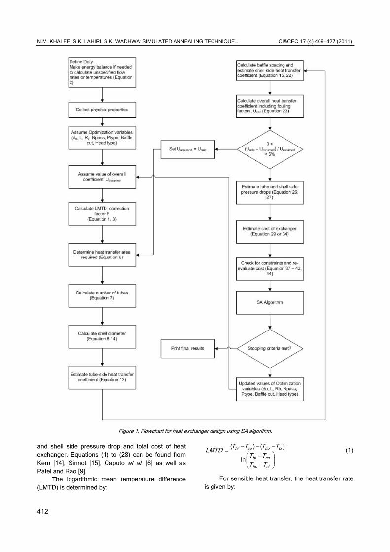
The entire process is schematized in Figure 1.

User input. Following parameters are required as a user defined input to calculate the heat exchanger area:

1. Mass flow rate and inlet/outlet temperatures of shell side and tube side fluids.

2. Thermophysical properties of both fluids, e.g., density, viscosity, heat capacity, thermal conductivity.

3. Fouling resistances, Rfoul, shell and Rfoul, tube. Input optimization variables. The optimization

variables, with values assigned iteratively by the opti-mization techniques (e.g. SA) are given in Table 1.

Calculation sequence

1. Assume overall heat transfer coefficient based on type of shell and tube side fluid.

2. Based on the actual values of the design specifications and on the current values of the opti-mization variables, the exchanger design routine de-termines the values of the shell side and tube side heat transfer coefficients, the overall exchanger area, the number of tubes, the shell diameter and tube side and shell side flow velocities, thus defining all cons-tructive details of the exchanger satisfying the as-signed thermal duty specifications.

3. Overall actual heat transfer coefficient is then calculated and compared with the assumed values of U.

4. If the difference between assumed and ac-tual values is within 0.5%, then algorithm goes to the next step. Otherwise it assigns new Uassumed = Ucalc and iterates the step 2 until the Uassumed and Ucalc values are within 0.5% agreement.

5. The computed values of flow velocities and the constructive details of the exchanger structure are then used to evaluate the cost objective function. The optimization algorithm, based on the value of the ob-jective function, updates the trial values of the optimi-zation variables which are then passed on to the de-sign routine to define a new architecture of the heat exchanger. The process is iterated until a minimum of the objective function is found or a prescribed conver-gence criterion is met.

Heat exchanger design procedure

This section describes step by step calculation procedure to evaluate heat exchanger area, tube side


412

and shell side pressure drop and total cost of heat exchanger. Equations (1) to (28) can be found from Kern [14], Sinnot [15], Caputo et al. [6] as well as Patel and Rao [9].

The logarithmic mean temperature difference (LMTD) is determined by:

( ) ( )

ln

hi co ho ci

hi co

ho ci

T T T TLMTD

T TT T

− − −= − −

(1)

For sensible heat transfer, the heat transfer rate is given by:

Figure 1. Flowchart for heat exchanger design using SA algorithm.


413

( )h ph hi hoQ m C T T= − (2)

The correction factor, F, for the flow configuration involved is found as a function of dimensionless tem-perature ratio for most flow configurations of:

2

2

1ln1 1

1 ln(2 ( 1 1))

PR PRFR P R R

−+ −=

− − + − + (3)

where the correction coefficient R is given by:

hi ho

co ci

T TR

T T−=−

(4)

Efficiency P is given by:

co ci

hi ci

T TP

T T−=−

(5)

Assuming the overall heat transfer coefficient Uassumed, the heat exchanger surface S is computed by:

assumed

QS

U FLMTD= (6)

Tube side calculations. Number of tubes, Nt, and tube bundle diameter, Db, are calculated as follows:

0t

SN

d Lπ= (7)

1

1

01

nt

bN

D dK

=

(8)

where K1 and n1 are coefficients that take values ac-cording to flow arrangement and number of passes as per table given by Sinnot [15].

Velocity through tubes is found by:

π ρ=

2

( )

4

tt

tt t

m nv

Nd (9)

The Darcy friction factor ft is calculated as fol-lows:

−= − 2(1.82log 10 1.64)tRetf (10)

where Ret is the tube side Reynolds number and given by:

ρμ

= t t it

t

v dRe (11)

where di is the inside diameter of tube and for sim-plicity kept constant as di = 0.8d0 in this work. How-ever, for more rigorous calculations, instead of keep-ing it constant, variable pipe thickness can be used from tables of tube manufacturers: schedules 40 or 80 or standard tubing gages: B.W.G. and Stub’s gage.

Prt is the tube side Prandtl number given by:

μ= t pt

tt

CPr

k (12)

According to flow regime, the tube side heat transfer coefficient (ht) is computed from following correlation for Ret ≤ 10000:

( )−= +

+ −0.67

1/2 2/3

( / 8) Re 1000[ (1 ) ]1 12.7( / 8) ( 1)

t t tt it

i t t

f Prk dh

d f Pr L (13)

and for Ret > 10000:

μμ

= 0.8 1/3 0.140.027 ( )t tt t t

o wt

kh Re Pr

d (14)

Shell side calculation

Clearance between tube bundle diameter and shell diameter is calculated from the figure given by Sinnot [15] for different head types as follows:

Table 1. Search optimization variables and their options

Optimization variable

Variable notation

Variable name Total options

available Corresponding options

x1 d0 Tube diameter, m 12 [0.00635, 0.009525, 0.0127, 0.01905, 0.022225, 0.0254, 0.03175, 0.0381, 0.04445, 0.0508, 0.05715, 0.0635].

x2 L Tube length, m 8 [1.2192 1.8288 2.4384 3.048 3.6576 4.8768 6.096 6.7056 7.3152]

x3 Rb Ratio of baffle spacing to shell diameter, (-)

17 [0.2 ,0.25, 0.3, 0.35, 0.4, 0.45, 0.5 ,0.55, 0.6 ,0.65, 0.7, 0.75, 0.8, 0.85, 0.9, 0.95, 1]

x4 Npass Number of tube pass, (-) 5 1-1, 1-2, 1-4, 1-6, 1-8

x5 Ptype Type of pitch, (-) 2 Triangular and square

x6 Headtype Head type, (-) 4 Fixed tube sheet or U tube, outside packed head, split ring floating head, and pull through floating head

x7 Bafflecut Baffle cut, % 4 [15, 25, 35, 45]


414

Clearance s b bD D mD c= − = +

where m and c are empirical constants and assume following values for different head type:

– fixed and U tube (0.01, 0.008), outside packed head (0.0, 0.038), split ring floating head (0.027, 0.0446), pull through floating head (0.009, 0.0862).

Baffle spacing is calculated as:

B = RbsDs (15)

Cross-sectional area normal to flow direction is determined by:

= − 0 (1 )a st

dS D B

P (16)

where Pt is tube pitch and given by Pt = 1.25 d0. Flow velocity for shell side can be obtained from:

ρ= ( )

ss

s a

mv

S (17)

Reynolds number and Prandtl number for shell side can be calculated as:

μ= s s

ss a

m DeRe

S (18)

μ= s ps

ss

CPr

k (19)

where Des is the shell hydraulic diameter and com-puted as:

– For triangular pitch:

( )ππ

−=

2 20

0

4(0.43 0.5 / 4 )

0.5t

s

S dDe

d (20)

– For square pitch:

( )ππ

−=

2 20

0

4( / 4 )

t

s

S dDe

d (21)

Kern’s formulation for segmental baffle shell-and-tube exchanger is used for computing shell side heat transfer coefficient hs:

=0.333

h s s ss

s

j K Re Prh

De (22)

where coefficient jh is calculated from the figure given by Sinnot [15] for different baffle cuts.

The following approximate equation was used:

Rech sj m=

where coefficients m and c are evaluated from figure given by Sinnot [15] for different baffle cuts, as fol-lows: 15% baffle cut (-6.7×10-8; 0.100067); 25% baffle cut (-4.5×10-8; 0.070045); 35% baffle cut (-4.4×10-8; 0.063044); 45% baffle cut (-3.4×10-8; 0.050034).

The overall heat transfer coefficient is calculated as follows:

=

+ + +

calc

1

1 1 ( )( )o

fs fts i t

Ud

R Rh d h

(23)

Compare and check the absolute error,%, between Uassumed and Ucalc as per following:

−= assumed calc

assumed

Error [%] 100 U U

U (24)

If error is more than 0.5%, assume new U as Uassumed = Ucalc and go back to Eq. (5) and recalculate everything until error reaches less than 0.5%.

When error is less than 0.5%, i.e., Uassumed and Ucalc is very near to each other proceeding for further calculations as follows:

– Exchanger area:

calc

QS

U FLMTD= (25)

The tube side pressure drop includes distributed pressure drops along the tube length and concen-trated pressure losses in elbows and in the inlet and outlet nozzles:

2

( 2.5)2t t

t ti

v LP f n

dρΔ = + (26)

The shell side pressure drop is given by:

2

2s s s

s ss

v L DP f

B DeρΔ = (27)

where fs is given by:

−= 0.1502s sf b Re (28)

where b0 = 0.72 valid for Res < 40000.

Objective function

Total cost Ctot is taken as the objective function, which includes capital investment (Ci), energy cost (Ce), annual operating cost (Co) and total discounted operating cost (Cod):

tot i odC C C= + (29)


415

Adopting Hall’s correlation, the capital invest-ment (Ci) is computed as a function of the exchanger surface area:

31 2

aiC a a S= + (30)

where a1 = 8000, a2 = 259.2 and a3 = 0.93 for ex-changer made with stainless steel for both shell and tubes.

The total discounted operating cost related to pumping power to overcome friction losses is com-puted from the following equation:

=0 eC PC H (31)

=

=+ 0

1 (1 )

ny

od xx

CC

i (32)

where pumping power P is computed from:

η ρ ρ= Δ + Δ1 ( )t s

t st s

m mP P P (33)

Based on all above calculations, total cost is computed from Eq. (29) for case studies 1 and 2. The cost objective function is kept exactly same as case study by GA approach by Caputo et al. [6] to enable the performance comparison of SA approach and GA approach.

However, for case study 3 the authors did not use same cost function in their case studies. Some of the authors [16] use total annual cost slightly diffe-rently as follows: the total cost consists of five com-ponents: the capital cost of the exchanger, the capital costs for two pumps, and the operating (power) costs of the pumps. The expression for the total annual cost is of the form:

ρ

ρ

= + + =

= + + + Δ +

+ + Δ

, ,( ) )

[( ) ( ( ) )

( ( ) )]

i f exc pumpT pump s

c etf a b e f t

t

ese f s

s

C A C C C

mA C C A C C P

mC C P

(34)

where Cexc, Cpump,t and Cpump,s are the capital costs for the exchanger, tube side and shell side pumps, respectively.

ηρ ρ

=Δ + Δ

1

( )od

t st s pow

t s

Cm m

P P C H (35)

tot i odC C C= + (36)

This new cost calculation is used in case study 3 to have a same basis for comparison of performance of SA approach and GA approach.

Constraints

Though the lowest cost exchanger is the main selection criterion for STHEs, this is not the only cri-terion for commercial plants. The concept of a good design involves aspects that cannot be easily des-cribed in a single economic objective function e.g. fouling suppression, maintenance ease, mechanical resistance, simplicity, flow distribution, potential tube vibration etc. These criteria, though subjective, have a profound effect on exchanger performance in com-mercial plants. These criteria are sometimes expres-sed as geometric and hydraulic and service cons-traints [17].

Geometric constraints

The STHE candidate must respect a series of geometric constraints, involving the following rules: the ratio between tube length and shell diameter must be between 3 and 15, the ratio between baffle spa-cing and shell diameter must be between 0.2 and 1; the baffle spacing cannot be lower than 50 mm; the baffle spacing must obey the maximum unsupported span. These constraints can be represented by the following mathematical expressions:

≤ ≤ 3 / 5sL D (37)

≤ ≤0.2 1bsR (38)

≤ ≤ max 0.050 / 0.5 /s bs b sD R L D (39)

Velocity constraints

These constraints represent fluid velocity limits in order to reduce fouling and erosion problems. The tube and shell side velocity must obey lower and up-per bounds:

ν ν ν≤ ≤min max t t t (40)

ν ν ν≤ ≤min max s s s (41)

High velocities will give high heat transfer coef-ficients but also a high pressure drop. The velocity must be high enough to prevent any suspended so-lids settling, but not so high as to cause erosion. High velocities will reduce fouling. Plastic inserts are some-timesused to reduce erosion at the tube inlet. Typical design velocities are given below [15].

Liquids. Tube-side, process fluids: 1 to 2 m/s, maximum 4 m/s if required to reduce fouling; water: 1.5 to 2.5 m/s; shell-side: 0.3 to 1 m/s.

Vapors. For vapors, the velocity used will de-pend on the operating pressure and fluid density; the lower values in the ranges given below will apply to high molecular weight materials; vacuum: 50 to 70


416

m/s; atmospheric pressure: 10 to 30 m/s; high pres-sure: 5 to 10 m/s.

In this work, the following constraints were im-posed on objective function:

≤ ≤ ≤ ≤1 2 m/s and 0.3 1 m/s t sv v

Service constraints

The hydraulic requirements of the service are represented by upper bounds on the pressure drop of both streams:

≤ max Δ Δt tP P (42)

≤ max Δ Δs sP P (43)

The values suggested below can be used as a general guide, and will normally give designs that are near the optimum. [15].

Liquids. For fluids having Viscosity <1 mN s/m2 maximum pressure drop: 35 kN/m2 [15]. For fluids having viscosities 1 to 10 mN s/m2, maximum pres-sure drop: 50-70 kN/m2 [15].

Gas and vapors. High vacuum: 0.4-0.8 kN/m2; medium vacuum: 0.1×absolute pressure; 1 to 2 bar: 0.5×system gauge pressure; above 10 bar: 0.1×system gauge pressure.

For the present case study following constraints were imposed:

ΔPt ≤ 35000 Pa; ΔPs ≤ 35000 Pa

The prerequisite of a good design is to choose the lowest cost exchanger with standard dimensions (as per TEMA standard) while obeying the above constraints. Attempt has been made in this work to apply SA optimization technique to design a lowest cost heat exchanger with TEMA dimensions and sa-tisfying all of the above constraints.

However, the value of the constraints of pres-sure drop and velocity is dependent on the detailed design and very much problem specific. In this work, the values of constraints are selected as per general guidelines given by Sinnot [15] and the user is not restricted to adhere this value. The value of these constraints must be judiciously selected as they have a big impact on final solution and cost. In case the user does not have specific restriction on these va-lues, the constraints should be kept as broad as pos-sible. This will facilitate the lowest cost heat exchanger.

Handling the constraints

The original problem can be set as: Minimize Ctot(x) Subject to gi(x) ≥ 0 where i = 1, 2, m

where x is the vector of optimization variables (Table 1). The set of constraints g(x) corresponds to the inequalities given by Eqs. (37)–(43).

For implementation of the SA algorithm, we used a penalty function in the objective function, to provide the following objective function to be mini-mized [16].

( ) ( ) penalty( )totObj x C x x= + (44)

The penalty function accounts for the violation of the constraints such that:

2

1

0 if is feasible

Penalty( )( ) otherwise

m

i ii

xx

r g x=

=

(45)

where ri is a variable penalty coefficient for the ith constraint, ri varies according to the level of violation.

Simulated annealing: at a glance [22]

What Is simulated annealing?

The simulated annealing method is based on the simulation of thermal annealing of critically heated solids. When a solid (metal) is brought into a molten state by heating it to a high temperature, the atoms in the molten metal move freely with respect to each other. However, the movements of atoms get restric-ted as the temperature is reduced. As the tempera-ture reduces, the atoms tend to get ordered and fi-nally form crystals having the minimum possible inter-nal energy. The process of formation of crystals es-sentially depends on the cooling rate. When the tem-perature of the molten metal is reduced at a very fast rate, it may not be able to achieve the crystalline state; instead, it may attain a polycrystalline state having a higher energy state compared to that of the crystalline state. In engineering applications, rapid cooling may introduce defects inside the material. Thus, the tem-perature of the heated solid (molten metal) needs to be reduced at a slow and controlled rate to ensure proper solidification with a highly ordered crystalline state that corresponds to the lowest energy state (in-ternal energy). This process of cooling at a slow rate is known as annealing.

Procedure [22]

The simulated annealing method simulates the process of slow cooling of molten metal to achieve the minimum function value in a minimization prob-lem. The cooling phenomenon of the molten metal is simulated by introducing a temperature-like parame-ter and controlling it using the concept of Boltzmann’s probability distribution. The Boltzmann’s probability distribution implies that the energy (E) of a system in


417

thermal equilibrium at temperature T is distributed probabilistically according to the relation:

( )EkTP E e

−= (46)

where P(E) denotes the probability of achieving the energy level E, and k is called the Boltzmann’s cons-tant. Equation (46) shows that at high temperatures the system has nearly a uniform probability of being at any energy state. However, at low temperatures, the system has a small probability of being at a high-energy state. This indicates that when the search process is assumed to follow Boltzmann’s probability distribution, the convergence of the simulated anneal-ing algorithm can be controlled by controlling the tem-perature T. The method of implementing the Boltz-mann’s probability distribution in simulated thermody-namic systems, suggested by Metropolis et al. [18] can also be used in the context of minimization of functions. In the case of function minimization, let the current design point (state) be Xi, with the corres-ponding value of the objective function given by fi = = f(Xi). Similar to the energy state of a thermodynamic system, the energy Ei at state Xi is given by:

( )i i iE f f X= = (47)

Then, according to the Metropolis criterion, the pro-bability of the next design point (state) Xi+1 depends on the difference in the energy state or function va-lues at the two design points (states) given by:

1 1( ) ( )i i i iE E E f X f X+ +Δ = Δ − Δ = − (48)

The new state or design point Xi+1 can be found using the Boltzmann’s probability distribution:

1( ) min 1,E

kTiP E e

Δ−+

=

(49)

The Boltzmann’s constant serves as a scaling factor in simulated annealing and, as such, can be chosen as 1 for simplicity. Note that if ∆E ≤ 0, Eq. (49) gives P(Ei+1) = 1 and hence the point Xi+1 is always accepted. This is a logical choice in the context of mi-nimization of a function because the function value at Xi+1, fi+1, is better (smaller) than at Xi, fi, and hence the design vector Xi+1 must be accepted. On the other hand, when ∆E > 0, the function value fi+1 at Xi+1 is worse (larger) than the one at Xi. According to most conventional optimization procedures, the point Xi+1

cannot be accepted as the next point in the iterative process. However, the probability of accepting the point Xi+1, in spite of its being worse than Xi in terms of the objective function value, is finite (although it may be small) according to the Metropolis criterion.

Note that the probability of accepting the point Xi+1 is not same in all situations. As can be seen from Eq. (50), this probability depends on the values of ∆E and T. If the temperature T is large, the probability will be high for design points Xi+1 with larger function values (with larger values of ∆E = ∆f). Thus at high tempe-ratures, even worse design points Xi+1 are likely to be accepted because of larger probabilities. However, if the temperature T is small, the probability of accept-ing worse design points Xi+1 (with larger values of ∆E = = ∆f) will be small. Thus as the temperature values get smaller (that is, as the process gets closer to the optimum solution), the design points Xi+1 with larger function values compared to the one at Xi are less likely to be accepted.

1( )E

kTiP E e

Δ−+ = (50)

Algorithm [22]

The SA algorithm [22] can be summarized as follows. Start with an initial design vector X1 (iteration number i = 1) and a high value of temperature T. Ge-nerate a new design point randomly in the vicinity of the current design point and find the difference in function values:

1 1( ) ( )i i i iE f f f X f X+ +Δ = Δ − Δ = − (51)

If fi+1 is smaller than fi (with a negative value of ∆f), accept the point Xi+1 as the next design point. Otherwise, when ∆f is positive, accept the point Xi+1

as the next design point only with a probability exp( / )E kT−Δ . This means that if the value of a ran-domly generated number is larger than exp( / )E kT−Δ , accept the point Xi+1; otherwise, reject the point Xi+1. This completes one iteration of the SA algorithm. If the point Xi+1 is rejected, then the process of gene-rating a new design point Xi+1 randomly in the vicinity of the current design point, evaluating the corres-ponding objective function value fi+1, and deciding to accept Xi+1 as the new design point, based on the use of the Metropolis criterion, Eq. (50), is continued. To simulate the attainment of thermal equilibrium at every temperature, a predetermined number (n) of new points Xi+1 are tested at any specific value of the temperature T. Once the number of new design points Xi+1 tested at any temperature T exceeds the value of n, the temperature T is reduced by a pre-specified fractional value c (0 < c < 1) and the whole process is repeated. The procedure is assumed to have con-verged when the current value of temperature T is sufficiently small or when changes in the function va-lues (∆f) are observed to be sufficiently small. The choices of the initial temperature T, the number of


418

iterations n before reducing the temperature, and the temperature reduction factor c play important roles in the successful convergence of the SA algorithm. For example, if the initial temperature T is too large, it re-quires a larger number of temperature reductions for convergence. On the other hand, if the initial tempe-rature is chosen to be too small, the search process may be incomplete in the sense that it might fail to thoroughly investigate the design space in locating the global minimum before convergence. The tempe-rature reduction factor c has a similar effect. Too large a value of c (such as 0.8 or 0.9) requires too much computational effort for convergence. On the other hand, too small a value of c (such as 0.1 or 0.2) may result in a faster reduction in temperature that might not permit a thorough exploration of the design space for locating the global minimum solution. Si-milarly, a large value of the number of iterations n will help in achieving quasi equilibrium state at each tem-perature but will result in a larger computational effort. A smaller value of n, on the other hand, might result either in a premature convergence or convergence to a local minimum (due to inadequate exploration of the design space for the global minimum). Unfortunately, no unique set of values is available for T, n, and c that will work well for every problem. As per recommen-dation of Rao [22], the initial temperature T can be chosen as the average value of the objective function computed at a number of randomly selected points in the design space. The number of iterations n can be chosen between 50 and 100 based on the computing resources and the desired accuracy of solution. The temperature reduction factor c can be chosen be-tween 0.4 and 0.6 for a reasonable temperature re-duction strategy (also termed the cooling schedule). More complex cooling schedules, based on the ex-pected mathematical convergence rates, have been used in the literature for the solution of complex prac-tical optimization problems. In spite of all the research being done on SA algorithms, the choice of the initial temperature T, the number of iterations n at any spe-cific temperature, and the temperature reduction fac-tor (or cooling rate) c still remain an art and generally require a trial-and-error process to find suitable va-lues for solving any particular type of optimization problems. The SA procedure is shown as a flowchart in Figure 2 [22].

Features of the method

Some of the features of simulated annealing as found from literature [22] are as follows:

1. The quality of the final solution is not affected by the initial guesses, except that the computational effort may increase with worse starting designs.

2. Because of the discrete nature of the function and constraint evaluations, the convergence or transition characteristics are not affected by the continuity or differentiability of the functions.

3. For problems involving behavior constraints (in addition to lower and upper bounds on the design variables), an equivalent unconstrained function can be formulated as in the case of genetic algorithms.

Figure 2. Simulated annealing procedure [22].

SA implementation

The objective function is the minimization of HE cost Obj(x) given in Eq. (44) and x is a solution string representing a design configuration.


419

The design variable x1 takes 12 values for tube outer diameter in the range of 0.00635m to 0.0635m (corresponds to 0.25–2.5”; refer to Table 1 for exact discrete values); the variable x2 takes eight values of the various tube lengths in the range 1.2192m to 7.3152m represented by numbers 1 to 8; x3 takes seventeen values for the variable baffle spacing, in the range 0.2 to 1 times the shell diameter; x4 takes number of tube passes 1-1, 1-2, 1-4, 1-6, 1-8 repre-sented by numbers from 1 to 5; x5 represents the tube pitch - either triangular or square - taking two values represented by 1 and 2; x6 takes the shell head types: fixed tube sheet or U tube, outside packed head, split ring floating head, and pull through floating head re-presented by the numbers 1, 2, 3 and 4, respectively; x7 takes four values for the baffle cut in the range 15 to 45%.

In the present study, the geometric constraints, velocity and pressure drop on the fluids exchanging heat is considered to be the feasibility constraint. For a given design configuration, whenever any of the above constraints exceeds the specified limit, a high value for the heat exchanger cost is returned through penalty(x) function (refer Eq. (44)) so that as an in-feasible configuration it will be eliminated in the next iteration of the optimization routine. The total number of design combinations with these variables are 12×8×17×5×2×4×4 = 261120. This means that if an exhaustive search is to be performed it will take at the maximum 261120 function evaluations before arriving at the global minimum heat exchanger cost. So the strategy which takes few function evaluations is the best one. Considering minimization of heat exchanger cost as the objective function, simulated annealing technique is applied to find the optimum design confi-guration with geometry, velocity and pressure drop as the constraint.

The code was developed in a Matlab environ-ment. The main steps of the approach are shown in Figures 1 and 2.

Case studies

The effectiveness of the present approach using SA algorithm is assessed by analyzing three case studies.

Case 1: 4.34 MW duty, methanol- brackish wa-ter exchanger [15].

Case 2: 1.44 MW duty, kerosene-crude oil ex-changer [14].

Case 3: 4.54 MW duty, oil-cooling water ex-changer [19].

The first two case studies were analyzed by Caputo et al. [6] using GA approach and taken from literature [15,14]. The third case studies was analyzed by Ponce-Ortega et al. [16] using GA approach and taken from the literature [19-21].

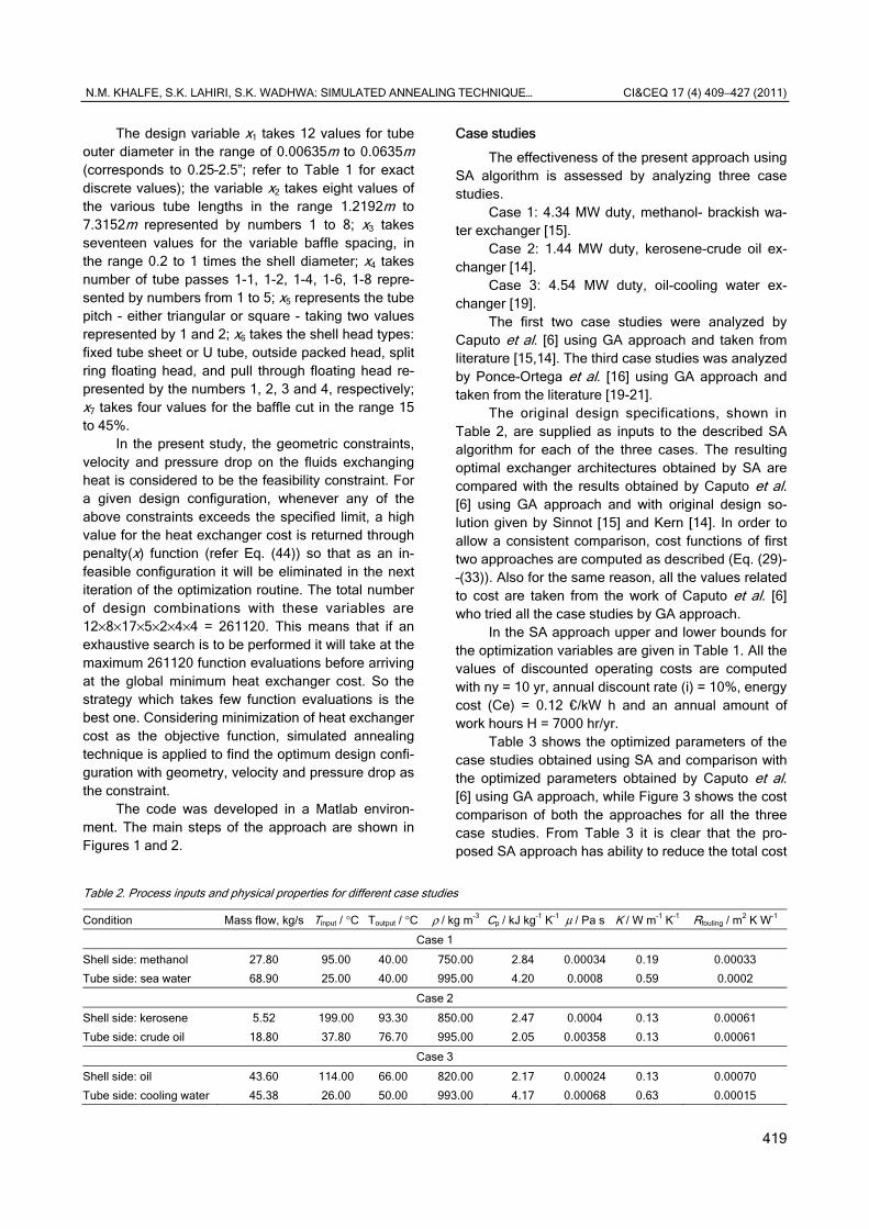
The original design specifications, shown in Table 2, are supplied as inputs to the described SA algorithm for each of the three cases. The resulting optimal exchanger architectures obtained by SA are compared with the results obtained by Caputo et al. [6] using GA approach and with original design so-lution given by Sinnot [15] and Kern [14]. In order to allow a consistent comparison, cost functions of first two approaches are computed as described (Eq. (29)- –(33)). Also for the same reason, all the values related to cost are taken from the work of Caputo et al. [6] who tried all the case studies by GA approach.

In the SA approach upper and lower bounds for the optimization variables are given in Table 1. All the values of discounted operating costs are computed with ny = 10 yr, annual discount rate (i) = 10%, energy cost (Ce) = 0.12 €/kW h and an annual amount of work hours H = 7000 hr/yr.

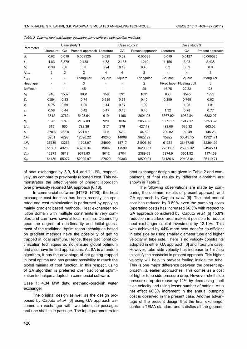
Table 3 shows the optimized parameters of the case studies obtained using SA and comparison with the optimized parameters obtained by Caputo et al. [6] using GA approach, while Figure 3 shows the cost comparison of both the approaches for all the three case studies. From Table 3 it is clear that the pro-posed SA approach has ability to reduce the total cost

Table 2. Process inputs and physical properties for different case studies

Condition Mass flow, kg/s Tinput / °C Toutput / °C ρ / kg m–3 Cp / kJ kg–1 K–1 μ / Pa s K / W m–1 K–1 Rfouling / m2 K W–1

Case 1

Shell side: methanol 27.80 95.00 40.00 750.00 2.84 0.00034 0.19 0.00033

Tube side: sea water 68.90 25.00 40.00 995.00 4.20 0.0008 0.59 0.0002

Case 2

Shell side: kerosene 5.52 199.00 93.30 850.00 2.47 0.0004 0.13 0.00061

Tube side: crude oil 18.80 37.80 76.70 995.00 2.05 0.00358 0.13 0.00061

Case 3

Shell side: oil 43.60 114.00 66.00 820.00 2.17 0.00024 0.13 0.00070

Tube side: cooling water 45.38 26.00 50.00 993.00 4.17 0.00068 0.63 0.00015


420

of heat exchanger by 3.9, 8.4 and 11.1%, respecti-vely, as compare to previously reported cost. This de-monstrates the effectiveness of present approach over previously reported GA approach [6,16].

In commercial software (HTFS, HTRI), the heat exchanger cost function has been recently incurpo-rated and cost minimization is performed by applying mainly gradient based methods. Heat exchanger so-lution domain with multiple constraints is very com-plex and can have several local minima. Depending upon the degree of non-linearity and initial guess, most of the traditional optimization techniques based on gradient methods have the possibility of getting trapped at local optimum. Hence, these traditional op-timization techniques do not ensure global optimum and also have limited applications. As SA is a random algorithm, it has the advantage of not getting trapped in local optima and has greater possibility to reach the global minima of cost function. In this respect, using of SA algorithm is preferred over traditional optimi-zation technique adopted in commercial software.

Case 1: 4.34 MW duty, methanol-brackish water exchanger

The original design as well as the design pro-posed by Caputo et al. [6] using GA approach as-sumed an exchanger with two tube side passages and one shell side passage. The input parameters for

heat exchanger design are given in Table 2 and com-parisons of final results by different algorithm are shown in Table 3.

The following observations are made by com-paring the optimum results of present approach and GA approach by Caputo et al. [6]. The total annual cost has reduced by 3.89% even the pumping costs (operating costs) has increased 66.3% with respect to GA approach considered by Caputo et al. [6] 15.8% reduction in surface area makes it possible to reduce heat exchanger capital investment by 12.19%. This was achieved by 44% more heat transfer co-efficient in tube side by using smaller diameter tube and higher velocity in tube side. There is no velocity constraints adopted in either GA approach [6] and literature case. However, tube side velocity has increase to 1 m/sec to satisfy the constraint in present approach. This higher velocity will help to prevent fouling inside the tube. This is one major difference between the present ap-proach vs. earlier approaches. This comes as a cost of higher tube side pressure drop. However shell side pressure drop decrease by 11% by decreasing shell side velocity and using lesser number of baffles. As a net effect 66.3% increment in the annual pumping cost is observed in the present case. Another advan-tage of the present design that the final exchanger conform TEMA standard and satisfies all the geomet-

Table 3. Optimal heat exchanger geometry using different optimization methods

Parameter Case study 1 Case study 2 Case study 3

Literature GA Present approach Literature GA Present approach Literature GA Present approach

d0 0.02 0.016 0.009525 0.025 0.02 0.00635 0.019 0.0127 0.009525

L 4.83 3.379 2.438 4.88 2.153 1.219 4.156 3.08 2.438

Rb 0.39 0.6 0.8 0.24 0.19 0.45 0.2 0.39 0.9

Npass 2 2 2 4 4 2 4 4 2

Ptype - - Triangular Square Square Triangular Square Square triangular

Headtype - - 3 - - 2 Fixed tube Floating pull 3

Bafflecut - - 45 - - 25 16.75 22.82 25

Nt 918 1567 3031 158 391 1831 838 1545 1992

Ds 0.894 0.83 0.74 0.539 0.63 0.40 0.899 0.769 0.62

vt 0.75 0.69 1.00 1.44 0.87 1.02 1 1.26 1.01

vs 0.58 0.44 0.42 0.47 0.43 0.46 1.32 0.78 0.77

ht 3812 3762 5428.64 619 1168 2604.93 5567.92 6062.84 6382.07

hs 1573 1740 2137.09 920 1034 2053.66 1009.17 1247.17 2353.52

Ucalc 615 660 782.36 317 376 427.48 483.06 535.32 663.02

S 278.6 262.8 221.07 61.5 52.9 44.52 200.02 180.49 145.26

ΔPt 6251 4298 12690.22 49245 14009 9622.99 15822 30543.15 12321.71

ΔPs 35789 13267 11708.97 24909 15717 21906.50 61354 36467.05 32364.92

Ci 51507 49259 43250.34 19007 17599 16200.57 27311.7 25902.32 24945.11

Cod 12973 5818 9679.63 8012 2704 2389.63 3874.9 3501.52 1174.59

Ctot 64480 55077 52929.97 27020 20303 18590.21 31186.6 29403.84 26119.71


421

ric, velocity and pressure drop constraints. In earlier GA approach [6] no such geometric, velocity and pressure drop constraints are imposed. These cons-traints are very much necessary in industrial scenario and ensure smooth functioning of heat exchanger in actual shop floor. Also in GA approach by Caputo et al. [6] the design variables (tube diameter, shell dia-meter etc.) are considered as continuous variable (as opposed to discrete variable which conforms TEMA standard considered in present case) and thus the final optimum solution may not conform TEMA stan-dard. In this respect, the solutions obtained by pre-sent approach are much more preferable than that of GA approach. However, these limitations can be re-moved from GA approach by following the advanced constraints and corresponding modeling methodology adopted in the present approach.

It was reported by Caputo et al. [6] that the objective function converges within about 15 genera-tions (each generations have 70 function calls as per 70 population) for this case against 703 function calls by SA algorithm to reach convergence. This shows for this case study, SA converges faster than GA with less number of function call. However this observation is limited to this case only and cannot be generalized. As the execution time is very negligible (1.5 s in Pen-tium 4 processors) in such type of design, the exten-sive exploration of solution space and goodness of the final solutions (i.e., least cost design) is more important here.

Case 2: 1.44 MW duty, kerosene crude oil exchanger

The original design as well as the design pro-posed by Caputo et al. [6] using GA approach as-sumed an exchanger with four tube side passages (with square pitch pattern) and one shell side pas-sage. The same configuration is not retained in the present approach and number of tube passes and pitch pattern are kept as a free optimization variable. The input parameters for heat exchanger design are given in Table 2 and comparisons of final results by different algorithm are shown in Table 3. It is ob-served that in this case higher tube side flow velocity increases the tube side heat transfer coefficient by 123%. A 13.69% increment in overall heat transfer coefficient is observed in the present case because of the combined increment in tube side and shell side heat transfer coefficient. As a result of high overall heat transfer coefficient, a reduction of 15.83% in heat exchanger area and reduction of 43% in heat ex-changer length is observed compared to GA approach considered by Caputo et al. [6]. The capital invest-ment is decreased by 7.94% and pumping cost also reduced by 11.62%. Reduction of tube passes from 4 to 2 and 43% reduction of tube length reduce the tube side pressure drop by 31.3%. However higher shell side velocity and lower diameter of shell makes the pressure drop of shell side more than calculated by GA. Overall 8.43% reduction in total annual cost is observed using this approach as compared to the GA approach considered by Caputo et al. [6].

Figure 3. Cost comparisons.


422

Case 3: 4.54 MW duty, oil- cooling water exchanger

To demonstrate the effectiveness of SA tech-nique, one more case study is considered which was originally analyzed by Serna and Jimenez [19], and later on improved by Ponce-Ortega et al. [16] using GA approach. The input parameters for heat ex-changer design are given in Table 2 and comparisons of final results by different algorithm are shown in Table 3. For comparison of the results, cost function (refer Eq (34)–(36)) and all the values related to cost taken from Ponce-Ortega et al. [16] are as follows:

Capital cost of exchanger ($) =

+ 0.8130000 750S (52)

Capital cost of pump ($) = ρ

+ Δ +0.68(2000 5( ) )tt

t

mP

ρ+ + Δ 0.68(2000 5( ) )s

ss

mP (53)

Cost of power ($/W Hr):

= 0.000045powC (54)

Pump efficiency:

η = 70% (55)

Plant operation (h/year):

H = 8000 (56)

Annualization factor (/year):

= 0.322fA (57)

The design proposed by Ponce-Ortega et al. [16] using GA approach assumed an exchanger with four tube side passages (with square pitch pattern) and one shell side passage. The same configuration is not retained in the present approach and considers the tube side passes a free variable. Results show increment of tube side and shell side heat transfer coefficient (5.26% on tube side and 88.7% on shell side) resulted in 23.85% increment in overall heat transfer coefficient in the present approach. The higher overall heat transfer coefficient results in 19.52% re-duction in heat exchanger area and 20.83% reduction in heat exchanger length in the present approach compared to GA approach. The capital investment is decreased by 3.69%. Less pressure drop in tube side (due to shorter tube length) and less pressure drop in shell side (due to less number of baffles) resulted in 66.45% reduction in pumping cost as compared to GA approach. In totality, the combined effect of capi-tal investment and operating costs results in 11.16% reduction in the total cost/year in the present ap-

proach compared to GA approach considered by Ponce-Ortega et al. [16].

Various alternatives of exchangers

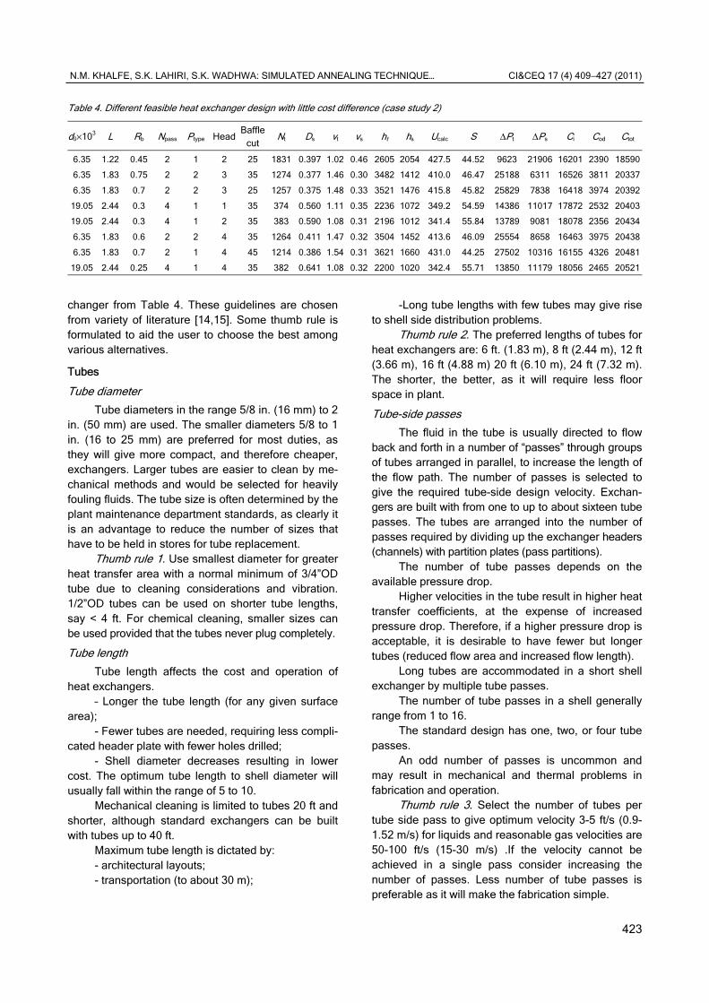
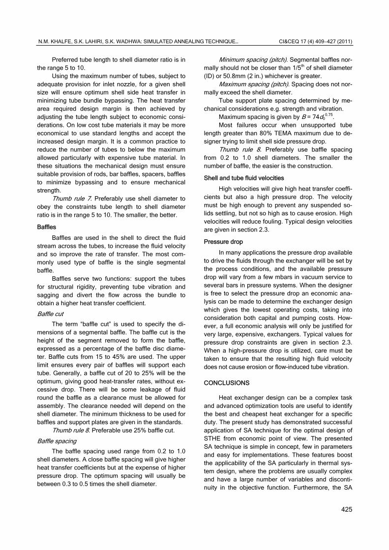
The solution space of cost objective function with multiple constraints is very much complicated with multiple local minima. Cost wise these local mi-nima may be very near to each other but geometri-cally represent complete different sets of exchangers. To assess these multiple local minima, the SA pro-gram was run 100 times with new starting guess every time. For case study 2, i.e., different sets of solutions vectors x is assumed in every run. Most of the times SA converged to global minima but sometimes it were found that it got stuck to local minima depending upon the complexity of solution space. All these feasible solutions were collected and solution within 5% of mi-nimum cost is presented in Table 4 for case study 2. From this table, it is clear that multiple heat exchanger configuration is possible with practically same cost or with little cost difference. All these solutions are feasible and the user has flexibility to choose any one of them based on his requirement and engineering judgment. For example, some users have very less space available in his company, so they may choose the lowest length heat exchanger and fixed tube head, as they have no space available to use a pull through heat exchanger. Selecting the best exchanger design from Table 4 is a combination of science and arts. Decision of best exchanger selection for a parti-cular service and industry is based on multiple criteria including costs. These criteria sometimes influence the best selection decision much more than the simple lowest cost criteria. Maintainability, ease of cleaning of tubes and shells, less fouling tendency, flow in-duced vibrations, less floor space requirement, com-pactness of design, etc., are some of these criteria which must be considered in an industrial scenario. The lowest cost exchangers are not always perform-ing best in actual shop floor. These criteria though very influential for final selection of exchanger are often qualitative and difficult to express quantitatively. It requires designer experience, engineering judg-ment, customer requirements and normally very prob-lem specific. Following section describes some of the criteria which can facilitate the user to select the best exchanger for his case studies. These criteria are col-lected from literatures and based on experience of designers. The final decision is dedicated to the user.

Practical design considerations to find the best exchanger

This section describes some of the practical de-sign criteria to help the user to choose the best ex-


423

changer from Table 4. These guidelines are chosen from variety of literature [14,15]. Some thumb rule is formulated to aid the user to choose the best among various alternatives.

Tubes

Tube diameter

Tube diameters in the range 5/8 in. (16 mm) to 2 in. (50 mm) are used. The smaller diameters 5/8 to 1 in. (16 to 25 mm) are preferred for most duties, as they will give more compact, and therefore cheaper, exchangers. Larger tubes are easier to clean by me-chanical methods and would be selected for heavily fouling fluids. The tube size is often determined by the plant maintenance department standards, as clearly it is an advantage to reduce the number of sizes that have to be held in stores for tube replacement.

Thumb rule 1. Use smallest diameter for greater heat transfer area with a normal minimum of 3/4”OD tube due to cleaning considerations and vibration. 1/2”OD tubes can be used on shorter tube lengths, say < 4 ft. For chemical cleaning, smaller sizes can be used provided that the tubes never plug completely.

Tube length

Tube length affects the cost and operation of heat exchangers.

– Longer the tube length (for any given surface area);

- Fewer tubes are needed, requiring less compli-cated header plate with fewer holes drilled;

- Shell diameter decreases resulting in lower cost. The optimum tube length to shell diameter will usually fall within the range of 5 to 10.

Mechanical cleaning is limited to tubes 20 ft and shorter, although standard exchangers can be built with tubes up to 40 ft.

Maximum tube length is dictated by: - architectural layouts; - transportation (to about 30 m);

-Long tube lengths with few tubes may give rise to shell side distribution problems.

Thumb rule 2. The preferred lengths of tubes for heat exchangers are: 6 ft. (1.83 m), 8 ft (2.44 m), 12 ft (3.66 m), 16 ft (4.88 m) 20 ft (6.10 m), 24 ft (7.32 m). The shorter, the better, as it will require less floor space in plant.

Tube-side passes

The fluid in the tube is usually directed to flow back and forth in a number of “passes” through groups of tubes arranged in parallel, to increase the length of the flow path. The number of passes is selected to give the required tube-side design velocity. Exchan-gers are built with from one to up to about sixteen tube passes. The tubes are arranged into the number of passes required by dividing up the exchanger headers (channels) with partition plates (pass partitions).

The number of tube passes depends on the available pressure drop.

Higher velocities in the tube result in higher heat transfer coefficients, at the expense of increased pressure drop. Therefore, if a higher pressure drop is acceptable, it is desirable to have fewer but longer tubes (reduced flow area and increased flow length).

Long tubes are accommodated in a short shell exchanger by multiple tube passes.

The number of tube passes in a shell generally range from 1 to 16.

The standard design has one, two, or four tube passes.

An odd number of passes is uncommon and may result in mechanical and thermal problems in fabrication and operation.

Thumb rule 3. Select the number of tubes per tube side pass to give optimum velocity 3-5 ft/s (0.9-1.52 m/s) for liquids and reasonable gas velocities are 50-100 ft/s (15-30 m/s) .If the velocity cannot be achieved in a single pass consider increasing the number of passes. Less number of tube passes is preferable as it will make the fabrication simple.

Table 4. Different feasible heat exchanger design with little cost difference (case study 2)

d0×103 L Rb Npass Ptype Head Baffle

cut Nt Ds vt vs ht hs Ucalc S ΔPt ΔPs Ci Cod Ctot

6.35 1.22 0.45 2 1 2 25 1831 0.397 1.02 0.46 2605 2054 427.5 44.52 9623 21906 16201 2390 18590

6.35 1.83 0.75 2 2 3 35 1274 0.377 1.46 0.30 3482 1412 410.0 46.47 25188 6311 16526 3811 20337

6.35 1.83 0.7 2 2 3 25 1257 0.375 1.48 0.33 3521 1476 415.8 45.82 25829 7838 16418 3974 20392

19.05 2.44 0.3 4 1 1 35 374 0.560 1.11 0.35 2236 1072 349.2 54.59 14386 11017 17872 2532 20403

19.05 2.44 0.3 4 1 2 35 383 0.590 1.08 0.31 2196 1012 341.4 55.84 13789 9081 18078 2356 20434

6.35 1.83 0.6 2 2 4 35 1264 0.411 1.47 0.32 3504 1452 413.6 46.09 25554 8658 16463 3975 20438

6.35 1.83 0.7 2 1 4 45 1214 0.386 1.54 0.31 3621 1660 431.0 44.25 27502 10316 16155 4326 20481

19.05 2.44 0.25 4 1 4 35 382 0.641 1.08 0.32 2200 1020 342.4 55.71 13850 11179 18056 2465 20521


424

Tube arrangements

The tubes in an exchanger are usually arranged in an equilateral triangular, square, or rotated square pattern. The triangular and rotated square patterns give higher heat-transfer rates, but at the expense of a higher pressure drop than the square pattern. A square, or rotated square arrangement, is used for heavily fouling fluids, where it is necessary to mecha-nically clean the outside of the tubes.

Triangular pattern provides a more robust tube sheet construction. Square pattern simplifies cleaning and has a lower shell side pressure drop.

For the identical tube pitch and flow rates, the tube layouts in decreasing order of shell-side heat transfer coefficient and pressure drop are: 30, 45, 60 and 90°.

The 90° layout will have the lowest heat transfer coefficient and the lowest pressure drop.

Thumb rule 4. The square pitch (90 or 45°) is used when jet or mechanical cleaning is necessary on the shell side. In that case, a minimum cleaning lane of 1/4 in. (6.35 mm) is provided. The square pitch is generally not used in the fixed header sheet design because cleaning is not feasible. The triangular pitch provides a more compact arrangement, usually result-ing in smaller shell, and the strongest header sheet for a specified shell-side flow area. It is preferred when the operating pressure difference between the two fluids is large.

Tube pitch

The selection of tube pitch is a compromise between:

- close pitch (small values of Pt/do) for increased shell-side heat transfer and surface compactness;

- open pitch (large values of Pt/do) for decreased shell-side plugging and ease in shell-side cleaning.

Tube pitch PT is chosen so that the pitch ratio is 1.25 < Pt/d0 < 1.5.

When the tubes are too close to each other (Pt/do less than 1.25), the header plate (tube sheet) becomes too weak for proper rolling of the tubes and cause leaky joints.

Tube layout and tube locations are standardized for industrial heat exchangers.

However, these are general rules of thumb and can be “violated” for custom heat exchanger designs.

Thumb rule 5. Prefer to use Pt/d0 = 1.25 unless otherwise specified.

Head type

The simplest and cheapest type of shell and tube exchanger is the fixed tube sheet design. The main disadvantages of this type are that the tube

bundle cannot be removed for cleaning and there is no provision for differential expansion of the shell and tubes. As the shell and tubes will be at different tem-peratures, and may be of different materials, the diffe-rential expansion can be considerable and the use of this type is limited to temperature differences up to about 80 °C. In the other types, only one end of the tubes is fixed and the bundle can expand freely.

The U-tube (U-bundle) type requires only one tube sheet and is cheaper than the floating-head types; but is limited in use to relatively clean fluids as the tubes and bundle are difficult to clean. It is also more difficult to replace a tube in this type.

Exchangers with an internal floating head are more versatile than fixed head and U-tube exchan-gers. They are suitable for high-temperature differen-tials and, as the tubes can be rodded from end to end and the bundle removed, are easier to clean and can be used for fouling liquids. A disadvantage of the pull-through design is that the clearance between the outermost tubes in the bundle and the shell must be made greater than in the fixed and U-tube designs to accommodate the floating head flange, allowing fluid to bypass the tubes. The clamp ring (split flange de-sign) is used to reduce the clearance needed. There will always be a danger of leakage occurring from the internal flanges in these floating head designs. In the external floating head designs the floating-head joint is located outside the shell, and the shell sealed with a sliding gland joint employing a stuffing box. Be-cause of the danger of leaks through the gland, the shell-side pressure in this type is usually limited to about 20 bar, and flammable or toxic materials should not be used on the shell side.

Thumb rule 6. Preferably use fixed head type.

Shells

The British standard BS 3274 covers exchan-gers from 6 in. (150 mm) to 42 in. (1067 mm) dia-meter; and the TEMA standards, exchangers up to 60 in. (1520 mm). Up to about 24 in. (610 mm) shells are normally constructed from standard, close tolerance, pipe; above 24 in. (610 mm) they are rolled from plate. The shell diameter must be selected to give as close a fit to the tube bundle as is practical; to reduce bypassing round the outside of the bundle.

The design process is to fit the number of tubes into a suitable shell to achieve the desired shell side velocity 4 ft/s (1.219 m/s) subject to pressure drop constraints. Most efficient conditions for heat transfer are to have the maximum number of tubes possible in the shell to maximize turbulence.


425

Preferred tube length to shell diameter ratio is in the range 5 to 10.

Using the maximum number of tubes, subject to adequate provision for inlet nozzle, for a given shell size will ensure optimum shell side heat transfer in minimizing tube bundle bypassing. The heat transfer area required design margin is then achieved by adjusting the tube length subject to economic consi-derations. On low cost tube materials it may be more economical to use standard lengths and accept the increased design margin. It is a common practice to reduce the number of tubes to below the maximum allowed particularly with expensive tube material. In these situations the mechanical design must ensure suitable provision of rods, bar baffles, spacers, baffles to minimize bypassing and to ensure mechanical strength.

Thumb rule 7. Preferably use shell diameter to obey the constraints tube length to shell diameter ratio is in the range 5 to 10. The smaller, the better.

Baffles

Baffles are used in the shell to direct the fluid stream across the tubes, to increase the fluid velocity and so improve the rate of transfer. The most com-monly used type of baffle is the single segmental baffle.

Baffles serve two functions: support the tubes for structural rigidity, preventing tube vibration and sagging and divert the flow across the bundle to obtain a higher heat transfer coefficient.

Baffle cut

The term “baffle cut” is used to specify the di-mensions of a segmental baffle. The baffle cut is the height of the segment removed to form the baffle, expressed as a percentage of the baffle disc diame-ter. Baffle cuts from 15 to 45% are used. The upper limit ensures every pair of baffles will support each tube. Generally, a baffle cut of 20 to 25% will be the optimum, giving good heat-transfer rates, without ex-cessive drop. There will be some leakage of fluid round the baffle as a clearance must be allowed for assembly. The clearance needed will depend on the shell diameter. The minimum thickness to be used for baffles and support plates are given in the standards.

Thumb rule 8. Preferable use 25% baffle cut.

Baffle spacing

The baffle spacing used range from 0.2 to 1.0 shell diameters. A close baffle spacing will give higher heat transfer coefficients but at the expense of higher pressure drop. The optimum spacing will usually be between 0.3 to 0.5 times the shell diameter.

Minimum spacing (pitch). Segmental baffles nor-mally should not be closer than 1/5th of shell diameter (ID) or 50.8mm (2 in.) whichever is greater.

Maximum spacing (pitch). Spacing does not nor-mally exceed the shell diameter.

Tube support plate spacing determined by me-chanical considerations e.g. strength and vibration.

Maximum spacing is given by B = 74d00.75.

Most failures occur when unsupported tube length greater than 80% TEMA maximum due to de-signer trying to limit shell side pressure drop.

Thumb rule 8. Preferably use baffle spacing from 0.2 to 1.0 shell diameters. The smaller the number of baffle, the easier is the construction.

Shell and tube fluid velocities

High velocities will give high heat transfer coeffi-cients but also a high pressure drop. The velocity must be high enough to prevent any suspended so-lids settling, but not so high as to cause erosion. High velocities will reduce fouling. Typical design velocities are given in section 2.3.

Pressure drop

In many applications the pressure drop available to drive the fluids through the exchanger will be set by the process conditions, and the available pressure drop will vary from a few mbars in vacuum service to several bars in pressure systems. When the designer is free to select the pressure drop an economic ana-lysis can be made to determine the exchanger design which gives the lowest operating costs, taking into consideration both capital and pumping costs. How-ever, a full economic analysis will only be justified for very large, expensive, exchangers. Typical values for pressure drop constraints are given in section 2.3. When a high-pressure drop is utilized, care must be taken to ensure that the resulting high fluid velocity does not cause erosion or flow-induced tube vibration.

CONCLUSIONS

Heat exchanger design can be a complex task and advanced optimization tools are useful to identify the best and cheapest heat exchanger for a specific duty. The present study has demonstrated successful application of SA technique for the optimal design of STHE from economic point of view. The presented SA technique is simple in concept, few in parameters and easy for implementations. These features boost the applicability of the SA particularly in thermal sys-tem design, where the problems are usually complex and have a large number of variables and disconti-nuity in the objective function. Furthermore, the SA


426

algorithm allows for rapid solutions of the design pro-blems (as compare to exhaustive search of solution space by conventional design method) and enables to examine a number of alternative solutions of good quality, giving the designer more degrees of freedom in the final choice with respect to traditional methods. Important additional constraints, like geometric, velo-city and pressure drop constraints, usually ignored in previous optimization schemes, are included in order to approximate the solution to the design practice. The solutions to case studies taken from literature show that cost of heat exchangers of previously re-ported designs can be improved through the use of the approach presented in this work.

Nomenclature

a1 = numerical constant ($) a2 = numerical constant ($/m2) a3 = numerical constant aps = shell side pass area (m2) B = baffles spacing (m) Baffle_cut = Baffle cut () Cpow = energy cost ($/kWh) Ci = capital investment ($) Cl = clearance (m) Co = annual operating cost ($/yr) Cod = total discounted operating cost ($) Cps = Cp of shellside fluid (kJ/Kg K) Cpt = Cp of tubeside fluid (kJ/Kg K) Ctot = total annual cost ($) Des = equivalent shell diameter (m) Db = Tube bundle diameter (m) Ds = shell inside diameter (m) di = tube inside diameter (m) d0 = tube outside diameter (m) F = temperature difference correction factor fs = friction factor shell side ft = Darcy friction factor tube side H = annual operating time (h/yr) hs = convective coefficient shell side (W/m2K) ht = convective coefficient tube side (W/m2K) i = annual discount rate () jh = Parameter for Baffle Cut K1 = numerical constant Ks = thermal conductivity shell side (W/m K) Kt = thermal conductivity tube side (W/m K) L = tubes length (m) LMTD = mean logarithmic temperature difference (degC) ms = shell side mass flow rate (kg/s) mt = tube side mass flow rate (kg/s) n1 = numerical constant n = Number of passes (1, 2, 4, 6, 8)

Nf = tubes number ny = equipment life (yr) P = pumping power (W) Prs = Prandtl number (shell side) Prt = Prandtl number (tube side) Pt = tube pitch (m) Ptype = Pitch type ΔPs = shellside pressure drop (Pa) ΔPt = tubeside pressure drop (Pa) Q = heat duty (W) Rb = Baffle Spacing / Shell Diameter Ratio Res = Reynolds number (shell side) Ret = Reynolds number (tube side) Rfs = conductive fouling resistance shell side (m2K/W) Rft = conductive fouling resistance tube side (m2K/W) S = heat exchange surface area (m2) Sa = Cross-sectional area normal to flow direction Thi = inlet fluid temperature shell side (K) Tci = inlet fluid temperature tube side (K) Tho = outlet fluid temperature shell side (K) Tco = outlet fluid temperature tube side (K) U = overall heat transfer coefficient (W/m2K)

Greek symbols

vs = fluid velocity shell side (m/s) vt = fluid velocity tube side (m/s) μt = viscosity at tube wall temperature (Pa s) μwt = viscosity at core flow temperature (Pa s) ρs = fluid density shell side (kg/m3) ρts = fluid density tube side (kg/m3) η = overall pumping efficiency

REFERENCES

[1] P.D. Chaudhuri, M.D. Urmila, S.L. Jefery, Ind. Eng. Chem. Res. 36 (1997) 3685–3693

[2] S. Kirkpatrik, C.D. Gelatt, M.P. Vechhi, Science 220 (1983) 671-680

[3] D.E. Goldberg, Genetic algorithms in search, optimization, and machine learning, Addison-Wesley, Reading, MA, USA, 1989

[4] L. Davis, Handbook of genetic algorithms, Van Nostrand Reinhold, New York, 1991

[5] C.T. Manish, Y. Fu, M.D. Urmila, Ind. Eng. Chem. Res. 38 (1999) 456–467

[6] A.C. Caputo, P.M. Pelagagge, P. Salini, Appl. Therm. Eng. 28 (2008) 1151-1159

[7] R. Selbas, O. Kizikan, M. Reppich, Chem. Eng. Process 45 (2006) 268-275

[8] M. Fesanghary, E. Damangir, Soleimani I, Appl. Therm. Eng. 29 (2009) 1026-1031

[9] V.K. Patel, R.V. Rao, Appl. Therm. Eng. 30 (2010) 1417- –1425

[10] D. Johnson, C. Aragon, L. Mregeoch, C. Schevon, Oper. Res. 37 (1990) 865-892


427

[11] D. Johnson, C. Aragon, L. Mregeoch, C. Schevon, Oper. Res. 39 (1991) 378-406

[12] D. Johnson, C. Aragon, L. Mregeoch, C. Schevon, Opti-mization by Simulated Annealing: An experimental eva-luation, Part III: the travelling Salesman Problem. Unpub-lished Manuscript, 1992

[13] K.J. Bell, Heat Transfer Eng. 21 (2000) 1-2

[14] D.Q. Kern, Process Heat transfer, McGraw-Hill, New York, 1950, p. 161-167

[15] R.K. Sinnot, An introduction to chemical engineering de-sign – Chemical engineering series by J.M. Coulson and J.F. Richardson, 6, Pergamon Press, Oxford, 1989

[16] J.M. Ponce-Ortega, M. Serna, A. Jimenez, Appl. Therm. Eng. 29 (2009) 203-209

[17] A.H.L. Costa, E.M. Queiroz, Appl. Therm. Eng. 28 (2008) 1798-1805

[18] N. Metropolis, A. Rosenbluth, M. Rosenbluth, A. Teller, E. Teller, J. Chem. Phys. 21 (1953) 1087-1092

[19] M. Serna, A. Jimenez, Chem. Eng. Res. Des. 83(A5) (2005) 539-550

[20] F.T. Mizutani, F. L.P. Pessoa, E.M. Queiroz, S. Hauan, I.E. Grossmann, Ind. Eng. Chem. Res. 42 (2003) 4009– –4018.

[21] F.T. Mizutani, F. L.P. Pessoa, E.M. Queiroz, S. Hauan, I.E. Grossmann, Ind. Eng. Chem. Res. 42 (2003) 4019– –4027

[22] S.S. Rao, Engineering Optimization theory and practice, John Wiley & Sons, Inc., Hoboken, New Jersey, 2009.

NADEEM M. KHALFE

SANDIP KUMAR LAHIRI

SHIV KUMAR WADHWA

Jubail Industrial City, Saudi Arabia

NAUČNI RAD

TEHNIKA SIMULIRANOG KALJENJA U PROJEKTOVANJU RAZMENJIVAČA TOPLOTE MINIMALNIH TROŠKOVA

Zbog širokog korišćenja razmenjivača toplote u industrijskim procesima, minimizacija nji-

hovih troškova je važan cilj i za projektante i za korisnike. Tradicionalno projektovanje

se bazira na iterativnim postupcima koji postepeno menjaju projektne i geometrijske pa-

rameter da bi zadovoljili zadatate uslove i ograničenja razmene toplote. Iako se pokazao

dobrim, ovakav pristup zahteva dosta vremena i može da ne dovede do isplativog pro-

jekta pošto nikakvi troškovni kriterijumi nisu eksplicitno uzeti u obzir. Ovaj rad istražuje,

sa ekonomske tačke gledišta, korišćenje netradicionalne tehnike optimizacije, tzv. simuli-

rano kaljenje (SA), za optimizaciju razmenjivača toplote tipa „cevi u omotaču“. Optimiza-

cioni postupak uključuje izbor glavnih geomterijskih parametara, kao što su: prečnik i du-

žina cevi, rastojanje između pregrada, broj prolaza kroz cevi, raspored cevi, vrstu čeone

glave, visina pregrada i tako dalje, dok se minimiziranje ukupnih godišnjih troškova pos-

tavlja kao projektni cilj. Prikazana tehnika SA je jednostavna po koncepciji, sa malim

brojem parametara i jednostavna za implementaciju. Osim toga, SA algoritam istražuje

brzo kvalitet rešenja, dajući projektantu više stepeni slobode u konačnom izboru u od-

nosu na tradicionalne metode. Ova metodologija uzima u obzir geometrijska i operativna

ograničenja koja se uobičajeno preporučuju projektnim kodovima. Tri različite studije slu-

čaja su predstavljene da bi se pokazala efikasnost i tačnost predloženog algoritma. SA

pristup je u stanju da smanji ukupne troškove razmenjivača toplote u poređenju sa troš-

kovima dobijenim GA pristup koji je ranije publikovan.

Ključne reči: simulirano kaljenje; projektovanje razmenjivača toplote; optimiza-cija; prenos toplote; matematičko modelovanje.

nadeem m. khalfe simulated annealing technique to … · shiv kumar wadhwa jubail industrial city,...

Documents