nasa technical note nasa tj · nasa technical note nasa tj d-5501 0. / f ... ohio 441 35 9. ... cid...

NASA TECHNICAL NOTE N A S A TJ D-5501 0. /

f

INJECTION OF A N ATTACHED INVISCID JET AT AN OBLIQUE ANGLE TO A MOVING STREAM

by Murvin E. Goldstein a n d Willis Braan

Lewis Research Center Cleveland, Ohio

N A T I O N A L A E R O N A U T I C S A N D S P A C E A D M I N I S T R A T I O N W A S H I N G T O N , D . C. O C T O B E R 1 9 6 9

https://ntrs.nasa.gov/search.jsp?R=19690030531 2018-11-23T12:36:59+00:00Z

TECH LIBRARY KAFB, NM

19. Security Classi f . (o f t h i s report)

Unclassified

1. Report No.

NASA TN D-5501 4. T i t l e and Subt i t le

20. Security Classi f . (of th is page)

Unclassified

2. Government Accession No.

INJECTION OF AN ATTACHED INVISCID JET AT AN OBLIQUE ANGLE TO A MOVING STREAM

7. Author(sj

Marvin E. Goldstein and Willis Braun

Lewis Research Center National Aeronautics and Space Administration Cleveland, Ohio 441 35

9. Performing Organization Name and Address

2. Sponsoring Agency Name and Address

National Aeronautics and Space Administration Washington, D. C. 20546

5 . Supplementary Notes

I Illill UIII Ill I

3. Recipient 's Catalog No.

5 . Report Date

October 1969 6 . Performing Organization C,

8. Performing Organization R E-5106

io. Work Un i t No.

~~

129-01 11. Contract or Grant No.

13. Type o f Report and Per iod

Technical Note

14. Sponsoring Agency Code

6 . Abstract

An analytical solution has been obtained to the problem of a two-dimensional invic incompressible jet injected into a moving s t r eam from an orifice se t at an obliqui to the s t ream for the case where the jet does not separate f rom the downstream E the orifice. The solution is valid when the difference between the total p re s su re jet and the total p ressure in the main s t r eam is not too large. Typical flow patte presented to i l lustrate the effects of varying both the orifice angle and the total p: within the jet.

17. Key Wards (Suggested b y Author(s))

Jet injection Inviscid flow Conformal mapping

18. D is t r ibu t ion Statement

Unclassified - unlimited

lllllllllll I

*For sale by the Clearinghouse for Federal Scientific and Technical Information Springfield, Virginia 22151

INJECTION OF AN ATTACHED INVISCID JET AT AN OBLIQUE

ANGLE TO A MOVING STREAM

by M a r v i n E. Goldstein and Wi l l i s B r a u n

Lewis Research Center

SUMMARY

An analytical solution has been obtained to the problem of a two-dimensional inviscid, incompressible jet injected into a moving s t r eam from an orifice set at an oblique angle to the s t r eam for the case where the jet does not separate from the downstream edge of the orifice. in the jet and the total p re s su re in the main s t r eam is not too large. Typical flow pat- t e rns a r e presented to illustrate the effects of varying both the orifice angle and the total p ressure within the jet.

The solution is valid when the difference between the total p ressure

INTRODUCTION

The flow field resulting f rom the oblique penetration of a jet into a flowing s t r eam is of considerable interest in a number of fluid mechanical devices. Among these are ground-effects machines, jet flaps, wing fans, and fuel injection systems.

The dynamics of jet injection into moving s t r eams is by no means fully understood. However, a certain amount of insight into this phenomenon can be gained by considering the injection of two-dimensional inviscid jets into flowing s t r eams since flows of this type a r e simple enough to be amenable to mathematical analysis. It is realized that viscous effects can be significant in real flows. In order t o take viscous effects into ac- count, however, it is necessary to first perform an inviscid analysis and then modify the flow by superimposing viscous boundary layers. In any event, it is hoped that the inviscid analysis will reveal some of the significant features of the flow and thereby lead to an increased understanding of the phenomena involved. The work done along these lines to date is summarized in reference 1.

solution for the flow field resulting from a two-dimensional inviscid and incompressible In reference 1 a technique was developed and applied to obtain an explicit analytic

jet issuing from an orifice into a moving s t ream. The orifice was at an oblique angle to the s t r eam and it was assumed that the jet separates f rom the downstream edge of the orifice to form a stagnant wake. Since it is not possible to tell from the inviscid analysis whether the jet will separate, remain attached, o r form a separation bubble, it is also of interest t o consider the flow that would result if no separation occurred. Hence, in this report the techniques used in reference 1 are used to obtain a solution for the case where the jet does not separate from the downstream edge of the orifice. The flow configuration is shown in figure 1 (p. 5). Since no separation is allowed to occur, it is necessary to allow the velocity to become infinite at the downstream edge of the orifice. This condition is approximately realized in certain real flows. The usual method for handling this situation is to replace the boundary streamline by one which is close to it when interpreting the results (ref. 2). In the present case this corresponds to replacing the infinitely thin plate which forms the downstream edge of the orifice by one of finite thickness with a streamlined leading edge.

compressible. In addition, it will be required that in a certain sense (to be specified more precisely) the difference between the total p ressure in the jet and the total p res - s u r e in the main s t r eam be small. The upstream boundary of the jet is the streamline emanating from the upstream edge of the orifice.

the difference in total p re s su re between the jet and the mainstream. The zeroth-order solution corresponds to equal total pressures .

Since the boundary shapes for the first-order problem a r e unknown, a technique s imilar to that employed in thin airfoil theory is used to t ransform the first-order bound- a r y conditions to the zeroth-order boundary. theory of sectionally analytic functions.

plies to the case where the density of the fluid in the jet differs f rom that in the main- s t ream.

As in reference 1, the flow will be assumed to be two-dimensional, inviscid, and in-

The problem is solved by expanding the solutions in a small parameter related to

The solution is then obtained by using the

It is proved in the appendix of reference 1 that the solution obtained herein also ap-

SYMBOLS

A

a A/L

B

b ' B/z

horizontal distance between edges of orifice

vertical distance between edges of orifice

2

pres su re coefficient along slip line cPS

D*

4 H

h

I

J

1

M

0

0

P

'j

pa0

P. v. P

P O

p,

Q S

S .-

yQ T

TJ

U

flow regions in physical plane

regions in T-plane

asymptotic jet width

H/1

function defined by eq. (54)


characteristic length (set equal to Ho)


order symbol

order symbol

total p ressure in main s t r eam

total p ressure in jet

total p ressure in main s t r eam

Cauchy principal value

static pressure

static pressure at jet source ( f a r inside the orifice)

static pressure far upstream from jet

volume flow through jet

slip line in physical plane

distance along slip line

slip line in T-plane

intermediate variable, T = + iq

X-component of velocity

u/v, Y - component of velocity

velocity along slip line inside of jet

f r ee s t r eam velocity

v/v,

3

W

X

X

Y

Y

2

Z S

r Y

E

A

6

< rl

0

A

5 P

T

4,

\k

*

dimensionless complex potential, cp + i$

coordinate in physical plane

x/z

y/z

coordinate in physical plane

dimensionless complex physical coordinate, x + iy

dimensionless coordinate of points on slip line


dummy variable to replace q

Pj - P,

1 2 - PV, r) L

location of downstream edge of orifice in T-plane

defined in fig. 7

dimensionless complex conjugate velocity, u - iv

coordinate in T-plane


defined by eq. (58)

coordinate in T-plane

dens it y

dummy variable in T-plane

velocity potential

+/ l v,

Q/l v, s t r eam function

Subscripts :

0 zeroth-order quantity

1 first-order quantity

Supers c r ipt s :

S

4

value of quantity on slip line

I

+ -

value of quantity inside jet and orifice

value of quantity in main s t r eam

(overbar) complex conjugate -

ANALYSIS

Fo rmu lat ion and Boundary Conditions

It will be assumed that the flow is inviscid, incompressible, and irrotational. The The analysis is limited to the case in which jet configuration is illustrated in figure 1.

the difference between the total p ressure in the jet P s t r eam P, is not too large; or more specifically, to the case in which

and the total p ressure in the main j

where

P j - P, E -

1 2 2 -- PV,

p is the density of the fluid and V, is the velocity of the main s t r eam at infinity.

Figure 1. - J e t penetrating stream.

5

I .

Let Z be a convenient reference length which will be specified in the course of the analysis. The X and Y components of the velocity, U and V, respectively, will be made dimensionless by V,; and the s t r eam function \k and the velocity potential will be made dimensionless by V,Z. Thus, the dimensionless quantities u, v, Q, and (p a r e defined by

The dimensionless complex conjugate velocity 5 and the dimensionless complex potential W a r e defined, as usual, by

< = u - i v

and

With all lengths made dimensionless by 2 (Le . , x = X / 1 , y = Y/Z, a = A / 1 , b = B/1, and h = H/Z) the flow configuration is shown in the physical plane (with the complex variable z defined by z = x + iy) in figure 2.

The s t r eam of fluid issuing from the orifice formed by the two parallel walls HD and EH meets the main s t r eam at the point D and forms a commm streamline which is denoted by S in figure 2. The jet does not separate f rom the wall EH at the goint E but turns and flows back along EC. A s a result of using this model it is necessary to allow the velocity to become infinite at the point E. Points on the common stream-

s s s line will be denoted by z = x + iy .

anywhere within the flow field, it is necessary (as is shown in ref. 1) to allow the velocity to be discontinuous across S. For this reason the streamline S will be called the

n

n

.-

In order to satisfy the requirement that there be no discontinuities in static pressure

6

Y t D- G

G

H ~

Figure 2. - Physical plane (z-plane).

slip line. gion of the flow (i. e. , the main s t ream) by D-. Since the velocity (and as a conse- quence, the velocity potential) is discontinuous across S, it is convenient to use a super- sc r ip t + to denote the flow quantities inside the jet (i. e., in D+) and a superscript - t o denote those in the main s t ream.

The region within the jet and orifice is denoted by D+ and the remaining re-

Thus,

and

w+(z) for z E D+

W-(z) for z E D -

W(z) =

Then c+ and W+ a r e holomorphic in the interior of D+ and <- and W- a r e holomorphic in the interior of D-.

A repetition of the argument given in reference 1 shows that Bernoulli's equation implies that

I T"(ZS) P. - Po3

= E - IC-(zS)l2 = J c.

2 1 z - PV, 2

at every point zs of S. Since S is a common streamline to the internal and external flows, it is clear that f l ( z s ) and .%n W-(zs) a r e both constants. Moreover, the ar-

7

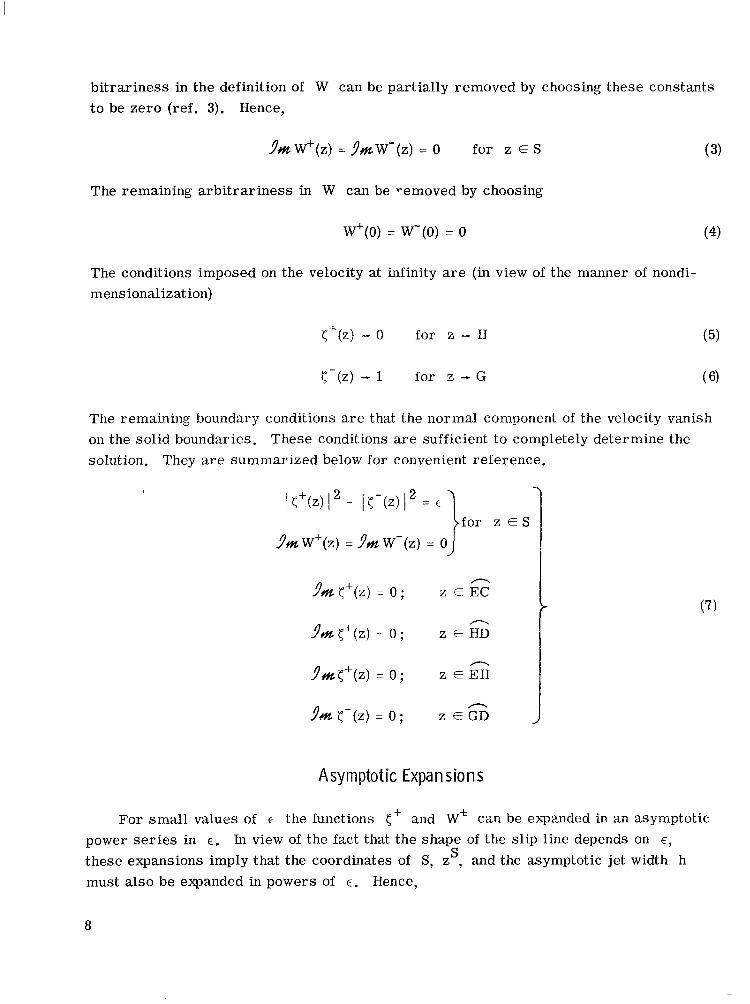
bitrariness in the definition of W can be partially removed by choosing these constm-ts t o be zero (ref. 3). Hence,

The remaining arbi t rar iness in W can be removed by choosing

(4) W+(O) = w-(o) = 0

The conditions imposed on the velocity at in€inity are (in view of the manner of nondi- mens ionalizat ion)

The remaining boundary conditions are that the normal component of the velocity vanish on the solid boundaries. These conditions are sufficient to completely determine the solution. They are summarized below for convenient reference.

94n y-(z) = 0 ; z €66

Asymptotic Expan si0 n s

J

For small values of E the functions ( * and W* can be expanded in an asymptotic power se r i e s in E . In view of the fact that the shape of the slip line depends on E ,

these expansions imply that the coordinates of S, z , and the asymptotic jet width h must also be expanded in powers of E. Hence,

S

8

1 f c = r O + € c l + . . .

I W * = w o + E W ; + . . .

i s s S 0 z = z + E Z 1 + . . .

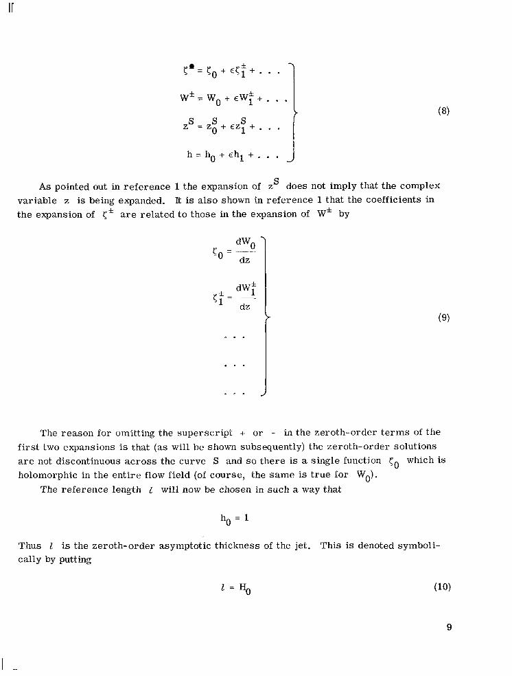
h = h 0 + € h i + . . . J As pointed out in reference 1 the expansion of zs does not imply that the complex

variable z is being expanded. the expansion of 5" are related to those in the expansion of W* by

It is also shown in reference 1 that the coefficients in

1 - dz s . .

0 . . 7 . L .

(9)

The reason for omitting the superscript + or - in the zeroth-order t e r m s of the f i r s t two expansions is that (as will be shown subsequently) the zeroth-order solutions a r e not discontinuous across the curve S and so there is a single function Po which is holomorphic in the entire flow field (of course, the s a m e is true for Wo).

The reference length 2 will now be chosen in such a way that

ho = 1

Thus 1 is the zeroth-order asymptotic thickness of the jet. This is denoted symboli- cally by putting

l = H 0 (10)

9

The last expansion (eq. (8)) is then

h = l + E h l + . . .

Zeroth-Order Solution

When the expansions (eq. (8)) a r e substituted into the boundary conditions (eqs. (4) to (7)) and only the zeroth-order t e r m s are retained, the following boundary conditions for the zeroth-order solution are obtained: First, the first boundary condition (eq. (7)) shows, as has already been anticipated, that the zeroth-order solution must be continu- ous across the sl ip line, and, hence, that it is characterized by functions which a r e holomorphic everywhere within the flow field. The remaining conditions show that

1 WO(O) = 0

94% wo(z;)= 0 )

0 for

z E E C

The conditions (eq. (12)) merely se rve to show that because of the manner in which the arbi t rary constants have been adjusted in the complex potential the streamline emanating f rom the point D is to be taken as the zero streamline.

Now the change in the s t r eam function across the jet must be equal to the volume flow rate through the jet. flow through the jet, and Aqo denotes the zeroth-order change in the s t r eam function across the jet, it is clear f rom the definition of s t r eam function that

Hence, if Qo denotes the dimensionless zeroth-order volume

10

. ,. .~ ... __.. - - . - - . . .. . . .-.. ._ . , , , . - . . -. . .. , ... . _. I I

The last boundary condition (eq. (13)) shows that far downstream in the jet (Le . , at the point C) the zeroth-order velocity goes to 1. In view of the normalization (eq. (11)) the asymptotic thickness of this portion of the jet must also be 1. It follows from these r e - marks that Q, = 1. Hence,

A$', = 1 (14)

Now the boundary value problem posed by the boundary conditions (eq. (13)) is a simple f ree streamline problem which can be readily solved by the Helmholtz-Kirchoff technique. Tn fact, the solution to this problem has already been car r ied out by Ehrich (ref. 4). His solution, however, is somewhat inconvenient for our purposes. Thus, it will be necessary to use a slightly different approach in order to obtain a zeroth-order solution which is in a convenient form to use for calculating the higher-order te rms . The procedure for obtaining the solution is (ref. 3), of course, t o draw the region of flow in the hodograph plane and in the complex potential plane, and then to find the ap- propriate mapping of these two planes into some convenient intermediate plane (say, the T-plane). The shapes of these regions can readily be deduced from the boundary conditions (eq. (13)), and they a r e shown in figures 3 and 4 (we have put W, = 'p, + iq, in fig. 3). The corresponding points in the various planes are designated by the same let- t e r s . The zeroth-order "slip line" is shown dashed in these figures since it does not correspond to a line of discontinuity and can therefore be ignored as far as obtaining the zeroth-order solution is concerned. The intermediate T-plane is chosen in such a way

H -1 C

Figure 3. - Zeroth-order complex potential plane (Wg-plane).

11

I .

1

-"0

Figure 4. - Zeroth-order hodograph (cO-plane).

7)

71 I Asymptote \, G

/ -- /

/--

I /

/ /

/ ' / ‘Lye

/

- A --

E

-1

C

Figure 5. - Intermediate plane (T-plane).

that the region of flow maps into the upper half plane in the manner indicated in figure 5. We shall denote the real a.nd imaginary par ts of the variable T by 5 and 7 , respectively. The region of the T-plane into which the zeroth-order flow field interior t o the jet maps is denoted by 9:, and the region of the T-plane into which the zeroth-order main s t r eam maps is denoted by -96. (which is being called for convenience the zeroth-order sl ip line even though no slip oc- durs in the zeroth-order solution) is denoted by Yo.

Simple applications of the Schwartz-Christoffel and linear fractional transformation (ref. 5) show that the mappings which properly transform the Wo-plane and the c0- plane into the upper half T-plane in the manner-indicated in the figures are respectively

The dividing line between these two regions

12

defined by

for n 2 0 d w O - l ___ T + l dT R T

and

m

or, performing the indicated integration,

1 W - - ( T + l + l n T ) - i for q 2 0 O - X

Since the Wo-plane and the T-plane are essentially the same as those of reference 1, the resul ts obtained therein can be used to show that the parametric equation for the zeroth-order sl ip line .!Po in the T-plane is

It follows from the first equation (9) that the points in the physical plane (fig. 2) are related to the points in the T-plane by

Substituting equations (15) and (16) into this formula and using the fact, indicated in fig- u r e 2, that the origin of the coordinate system in the physical plane is to be at the point D result in

1 A = -- T + (1 - A)ln T + - + (1 + A) + ( A - l ) i R '1 T

(19)

1 3

By definition (see figs. 2 and 5)

z(A) = a + ib

Hence, equation (19) shows

1 a + ib = -[(I - A ) h A + 2(1 + A)] + i ( A - 1) a

Therefore, on equating real arid imaginary parts,

I 1 a = -[(I - A ) h A + 2(1 + A)] a

b z A - 1

Formulation of First-Order Problem in Physical Plane

The mapping T -c Z defined by equation (19) maps the upper haif T-plane approximately into the region of flow in the physical plane. The domain 9; is mapped into the crosshatched region of the physical plane shown in figure 6 . The curve Yo is mapped into the dashed boundary So of this region. This region, of course, differs f rom the t rue interior of the jet whose boundary S is indicated by the solid line (curved) in fig- u r e 6 .

Now the first group of the boundary conditions (eq. (7)) is specified on the curve S in the physical plane, whose shape is not known at this stage of the solution. A s ex- plained in reference 1, however, these boundary conditions, correct to t e r m s of the order E , can be t ransferred to So by relating the values of <* and W* at an arbi- t r a r y point zs of S to their values at some neighboring point zo of So by performing S

Figure 6. - Comparison a s zeroth order and t rue jet boundaries i n physical plane.

14

a Taylor series expansion of these quantities about z;. Thus,

5 * s (z ) = 5 * s (Zo)+ (e) (A z;)+. . . z=zo dz

w * s (z ) = w * s (zo)+ 5 * s (Zo)(ZS - z;>+ * - *

As in reference 1 substitution of the asymptotic expansion (eq. (8)) into these Taylor series yields, after neglecting t e r m s of O(E ),

2

r 1

And these expressions relate the values of the dependent variables W* and C* at the points of the unknown boundary S to their values on the known boundary So with an e r r o r of order E . An easy calculation carr ied out in reference 1 shows that equation (21) implies

2

Finally, substituting the expansions (eqs. (22) and (23)) into the f i r s t group of bound- a r y conditions (eq. (?)) and equating the coefficients of E to the first power yields the following first-order boundary conditions on the slip line:

9m [W;(z;)+ %o(z;)z;] = 0

s s h [w;(z;) + PO(zO)~l] = 0

I

Thus, equations (24) t o (26) are the boundary conditions for the first-order solutions on the boundary S l l transferred' l to the.zeroth-order boundary So. Hence, the first-order boundary value problem has been transformed f rom one in which the shape of the boundaries is unknown to one in which it is known. Notice, however, that these boundary con-

S ditions involve the variables Wf, <f, and z l . But, <: is completely determined in t e r m s of Wf by the second equation (9). In view of this the conditions (eqs. (24) to (26)) may be thought of as two boundary conditions connecting the variable <; with the variable equation which determines z s once from (25) yields

ac ross So (or equivalently the variable wf with the variable W;) plus an are known. Thus, subtracting equation (26)

Then in view of the second equation (9), equations (24) and (27) are the boundary conditions on So which connect the solution c; in D+ with the solution r; in D-, and equation (25) se rves to determine z s once [; is known (actually zs will be determined in a slightly different fashion). It is shown in reference 1 that the boundary condition (eq. (27)) can be differentiated to obtain

Multiplying this by i and adding it to equation (24) yield the following single (complex) jump condition on So:

The boundary conditions for the remaining (solid) boundaries are easily deduced by substituting the f i r s t asymptotic expansion (eq. (8)) into expressions (5) and (6) and the second group of boundary conditions (eq. (7)) and equating the coefficients of E to the first power. Thus,

16

<;(z) - 0 z - H

< ; ( z ) - o z - G J

Solut ion of First-Order Boundary-Value Problem

The boundary conditions (eqs. (28) and (29)) completely determine a boundary-value problem (or more precisely, two boundary- value problems connected along the curve S ) fo r a holomorphic function in the region of flow in the physical plane. under the change of variable z -. T defined by equation (19) this boundary-value problem can be transformed into one in the upper half T-plane (fig. 5). in the T-plane are

However, 0

The boundary conditions

Clearly, the domains of definition of <+ and <- are 9; and .9;, respectively. It is convenient to work with the sectionally analytic function 0 defined on the upper half T- plane in t e r m s of c* by

17

O(T) = {

It follows from the boundary conditions (eq. (30)) that 8 must satisfy

where we have put

O+(T) - O-(T) = r(T)

9m o(( + io ) = o

for T € Y o

for --oo < 5 < +-oo

O(T) - 0 for T - -oo

Since can be no more singular than To, if the asymptotic expansion is to be uni- formly valid it follows that O must be bounded on the real axis.

The function 0 can now be constructed as follows: An investigation of the behavior of r(T) at T = 00 and T = -1 shows that it vanishes at these points like some power of T. Hence, the Plemelj formulas (ref. 6) show that the Cauchy integral

where the integration is to be performed along Yo in a counterclockwise direction

18

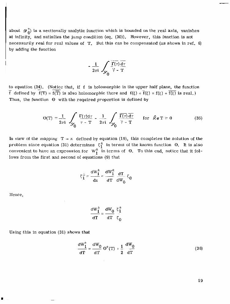
about 9;) is a sectionally analytic function which is bounded on the real axis, vanishes at infinity, and satisfies the jump condition (eq. (30)). However, this function is not necessarily real for real values of T. But this can be compensated (as shown in ref. 6) by adding the function

2ni J 7 - T

t o equation (34). f defined by f (T) = fo is also holomorphic there and f(5) +T(5) = f (5) + fo is real.) Thus, the function 0 with the required properties is defined by

(Notice that, if f is holomorphic in the upper half plane, the function -

In view of the mapping T - z defined by equation (19), this completes the solution of the problem since equation (31) determines ct in t e r m s of the known function 0. It is also convenient to have an expression for W; in t e r m s of 0. To this end, notice that it follows from the first and second of equations (9) that

* dWf - dWf dT c l = T - - - c o

dT dWo

Hence,

dT dT To

Using this in equation (31) shows that

d q d w 0 0 + (T) + - 1 - dWo dT d T 2 dT

19

Notice that z = 0 when T = -1 and, therefore, equation (4) implies that Wi(T) both vanish at T = -1. Hence, integrating equations (36) and (37) between -1 and T yields

1 d T + - WO(T) 2

f O+(T) - dWO dT

WfU) =

J- 1

(39) "0 O-(T) -

Wi(T) = 6' dT

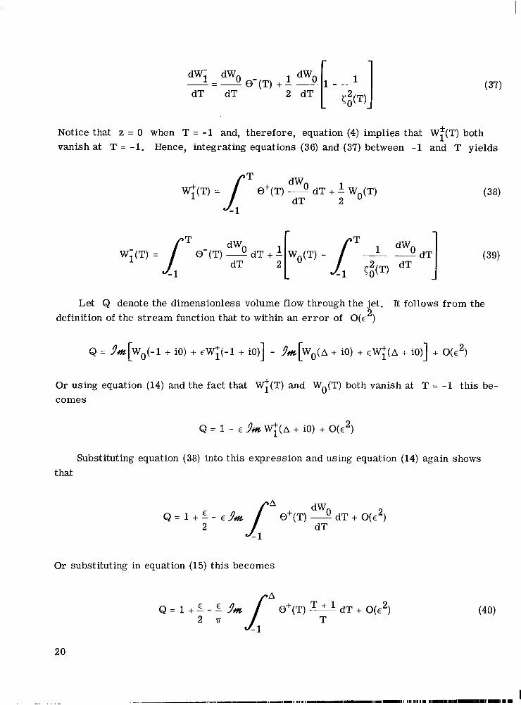
Let Q denote the dimensionless volume flow through the jet. It follows from the 2 definition of the s t ream function that to within an e r r o r of O(E )

Or using equation (14) and the fact that $(T) and Wo(T) both vanish at T = -1 this becomes

Substituting equation (38) into this expression and using equation (14) again shows that

A Q = l + f - ~ j m j f O+(T)- dWo dT + O(t2)

2 dT

Or substituting in equation (15) this becomes

J- 1

20

. ...

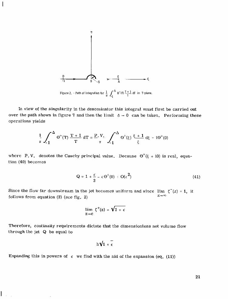
Figure 7. - Path of integration for 1 /" &(TI TA dT in T-plane. T 57 -1

In view of the singularity in the denominator this integral must first be carr ied out over the path shown in figure 7 and then the limit 6 - 0 can be taken. Performing these operations yields

where P. V. denotes the Cauchy principal value. Because of([ + io) is real, equation (40) becomes

Since the flow far downstream in the jet becomes uniform and since l im g - ( z ) = 1, it follows from equation (2) (see fig. 2) Z-CcJ

Therefore, continuity requirements dictate that the dimensionless net volume flow through the jet Q be equal to

Expanding this in powers of E we find with the aid of the expansion (eq. (11))

21

I -

= l + ~ - + h + . . . (: 1)

Hence, equating like powers of E in equations (41) and (42) shows that

hl = O+(O) (4 3)

Since equation (19) set up a one-to-one correspondence between points of the physical plane and points of the T-plane, it is clear that equations (31), (35), (38), and (39) can be used to compute the first-order perturbation to the velocity and s t r eam function at each point of the physical plane.

the streamline patterns, the most important quantities to be obtained from the analysis are the shapes of the curve S in the physical plane (see fig. 2). However, since the viscous spreading of the jet is controlled by the pressure (or equivalently, the velocity) distribution along the sl ip line S, that quantity is also of some importance. Hence, explicit formulas will now be obtained for these quantities by using the formulas previously derived.

In view of the fact that once the shape of the jet is known it is quite easy to sketch in

Computation of Boundary Values

In view of the one-to-one nature of the mapping involved it is clear that, if .hW+(z) = 0, then z must be a point on the streamline which passes through the point D in figure 2. In addition, since the velocity potential is increasing in the direction D - C along S, it is clear that, if /?e&(z) > /?eW+(O) = 0 (see eq. (4)), then z must be a point of the sl ip line S. It is clear that %n Wo(z$ = 0 and /?e Wo(zs) L 0 for any

S S S point zo E So. In view of these considerations it follows that the point zg= zo + E Z ~

will be on the first-order position of S if zs satisfies the equation

w + s (z ) = w o ( z q l + s ) 2

(44)

S + s It is clear from this equation that when zo = 0, W (z ) = 0, and that /?e W+(zs) - 00 as zo - 03. Hence, the point zs traverses the streamline S as zo t raverses the zeroth- order slip line So.

S S

22

By substituting equation (44) into the expansion (eq. (22)), the first-order distance z s from the zeroth-order sl ip line t o the slip line is found t o be *

where the fact has been used that the curve So in the physical plane is the conformal image under the mapping T - z defined in equation (19) of the curve Yo in the T- plane. This also shows that

(4 6) S 2 zs = Z(T) + EZ1 + o ( E ) for T E yo

S In addition, equation (23) shows that the magnitude of the velocity at each point z of the sl ip line is given to within t e r m s of order c2 by

Substituting equation (45) into (46) and substituting equation (38) into the resulting expression yield

where the integral can be taken along the curve Y o if S+(T) is interpreted as the limiting value of O(T) as T approaches Y o from within 9;.

It follows from the first equation (9) and equations (46), (48), and (31) that

O+(T) __ dWo dT dT dWO

1 2

= - + &(T) - ~

23

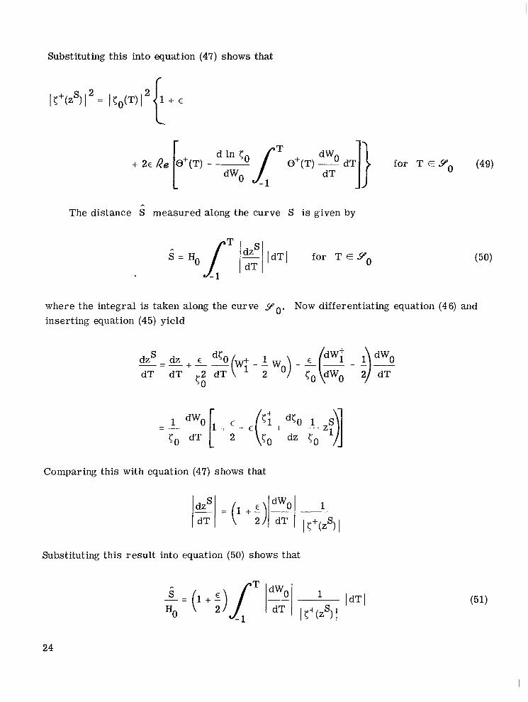
Substituting this into equation (47) shows that

f

A

The distance S measured along the curve S is given by

where the integral is taken along the curve yo. Now differentiating equation (46) and inserting equation (45) yield

+ - - 2

Comparing this with equation (47) shows that

Substituting this result into equation (50) shows that

24

All necessary resul ts have now been obtained. However, it is convenient t o rewrite some of these in more explicit form.

Explicit Formulas for Calculat ing Boundary Values

Substituting equation (1 6) into equation (33) yields

T - A g * T - A T T

r(T) = -i-

Or using equation (17)

where r(q) is used in place of r[-(q/sin ~ ) e - ~ ~ ] . Applying the Plenielj formulas (ref. 6) to equation (35) shows that

where the integration is to be performed in a counterclockwise direction along Yo. view of equation (24), however, this can be written as

In

where, for brevity, O+(q) is used in place of O+ [ (-q/sin q)e-’q]. Since

25

I

I I 1l1111l1l1l1ll111l111111l11ll1l11ll11l11

the foregoing equation can be written as

For T = 0 equation (35) becomes

S S Upon defining zo(q) and co(q) by

for 0 5" < n

sin 77

and using equations (15), (17), and (53), equation (46) becomes

(56)

where

26

and

for 0 < q < r

for 0 I y < r J(y) = -[(I 1 - y cot y ) 2 + y2] nY

Upon defining Vi(q) by

for O < _ q < r + s V;(d E v,15 (2 ) I

and using equations (15), (16), (17), and (53), equation (49) becomes

where

Let po be the pressure far inside the orifice (the point H in fig. 2). is zero there, it is clear that po = Pj. pressure at the point (xs, ys) on the slip line p(xs, ys) is given by

Since the velocity Hence, it follows from equation (2) that the

Hence, let the pressure coefficient on the sl ip line C be defined by PS

- - Po - P(XS, Ys)

1 2 2

cps - - PV,

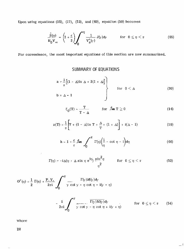
Upon using equations (15), (17), (53), and (60), equation (50) becomes

For convenience, the most important equations of this section are now summarized.

SUMMARY OF EQUATIONS

for ~ " T > _ o

1 A z(T) = - T + (1 - A ) h T + - + (1 + A) + i ( A - 1) 71 ' I T

h = 1 - f hz [' I?(.)(' - cot q - 71 77

2

2 for 0 < q < I T iq s in q r ( V ) = -iA(q + A sin 77 e ) __

?1

-~ w ) (r ) dv for 0 < q < 7r (54) y cot y - q cot q + i(y + q) 27ri

where

28

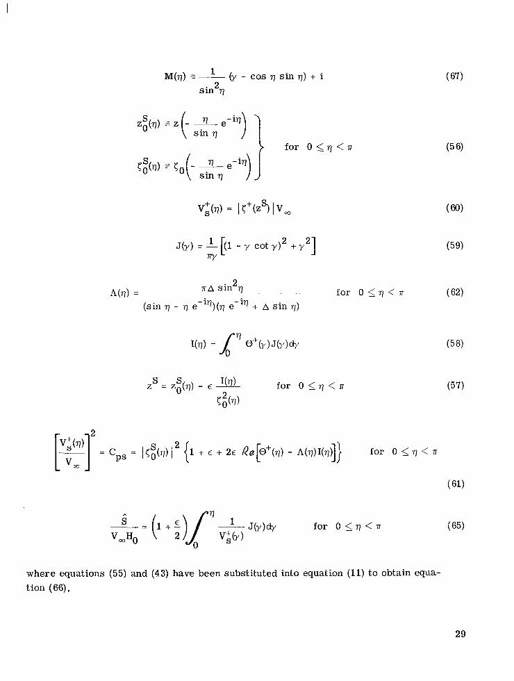
M(q) =_ - (y - cos 71 sin 7 ) + i 2 sin 17

\ for o < _ q < r

1

ny J(y) = - 11 - y cot y ) 2 + 7 2 1 (59)

where equations (55) and (43) have been substituted into equation (11) to obtain equation (66).

29

RESULTS AND DISCUSSION

The numerical calculations were performed by using complex arithmetic. Hence, there is no need to separate the rea l and imaginary par t s of the various formulas given in the preceding section, Equations (20) are used to calculate the orifice offset ratio B/A = b/a for various values of the parameter A. However, it is more convenient to present the resu l t s in t e r m s of the orifice orientation angle defined as tan-'B/A. A plot of the orifice angle against the parameter A is presented in figure 8. angle completely fixes the geometry of the problem. Hence, once the geometry of the orifice is set , the parameter A can be determined from figure 8. This parameter is the one which appears naturally in the formulas which a r e used to calculate the various physical quantities of interest. The only other parameter appearing in the problem is E

which gives a measure of the difference between the total p ressure in the jet and the total p ressure in the mainstream.

The orifice

This parameter is defined by equation (1) as

P j - Pw E =

1 2 2 - PVw

Equation (52) is used to calculate r(q) for various values of A and these values of r(q) are used together with equation (67) to calculate @+(e) and h for various values of

-3 k .1 I I 1 1 1 1 1 1 1 I I I l l l l l l 10 I I I 1 1 1 1 1 1 100

.01 T-plane parameter, A

Figure 8. - Dependence of or i f ice angle o n parameter A.

30

A from equations (54) and (66), respectively. All the physical quantities presented in the plots are determined by these latter two quantities.

jet thickness divided by the length of the orifice. Now for two-dimensional jets, the jet contraction ratio is defined as the asymptotic

Hence, the jet contraction ratio is

{A2 + B2 {a2 + b2

Substituting equations (20) and (66) into this formula gives the jet Contraction ratio as a function of A and E o r in view of figure 8 as a function of tan-'B/A and E .

resul ts are presented in figure 9. the separated jet discussed in reference 1, for positive values of the orifice angle small changes of E result in large changes in the contraction ratio, the effect becoming more marked as the orifice angle is increased. values of the orifice angle. However, this effect is not nearly so marked as that of reference 1. Figure 9 also shows that, as in the case of the separated jet, for a given orifice angle increasing E always results in an increase in the jet contraction ratio. T h i s increase is negligible, however, fo r orifice angles less than -1. 6 radians. Figure 9 shows that the jet contraction ratio is a maximum for an orifice angle of -1 . 2 radians and falls off markedly when the orifice angle is changed.

stituting equations (19), (16), and (58) into equation (57) and using definitions (56) and the

These It can be seen from figure 9 that, as in the case of

The opposite conclusion holds for negative

The parametric equations (with parameter q ) for the sl ip line are obtained by sub-

I

0- c .6 m, 0 c

c c 0 0

-3

Value of E

l -2

-. OS\

I 1 I \ L A 2 3 0

I -1 Orifice angle, tan-] BIA

Fi(;ure 9. - Jet contraction ratio.

31

I Ill I1 llll1111l1l1l1l.11lll11111l1 I

expression for O i ( ( ) discussed previously. The resulting expression determines the boundary of the jet. The shapes of the jet boundaries for various values of the param- eters E and B/A are shown in figures lO(a) t o (i). Figure lO(a) corresponds to a jet injected normal to the mainstream B = 0. Figures 10(b) t o (e) are for negative orifice angles (i. e., jet injected downstream) and figures lo(€) to (i) are for positive orifice angles (i. e., jet injected upstream). The configurations shown in figures lO(g) to (i) may be strongly modified by viscous effects. case of the separated jet discussed in reference 1, when the orifice angle is greater than or equal to ze ro a small change in the total p re s su re within the jet results in a fairly large change in both the jet penetration and jet thickness. This effect becomes more pronounced as the orifice angle is increased. However, the effect is not as marked as in the case of a separated jet. The figures also show that turning the jet into the main s t ream tends tc markedly decrease the flow in the jet, The extreme sensitivity of the flow configuration to E at large positive orifice angles indicates that the perturbation analysis will break down when the orifice angle is large enough.

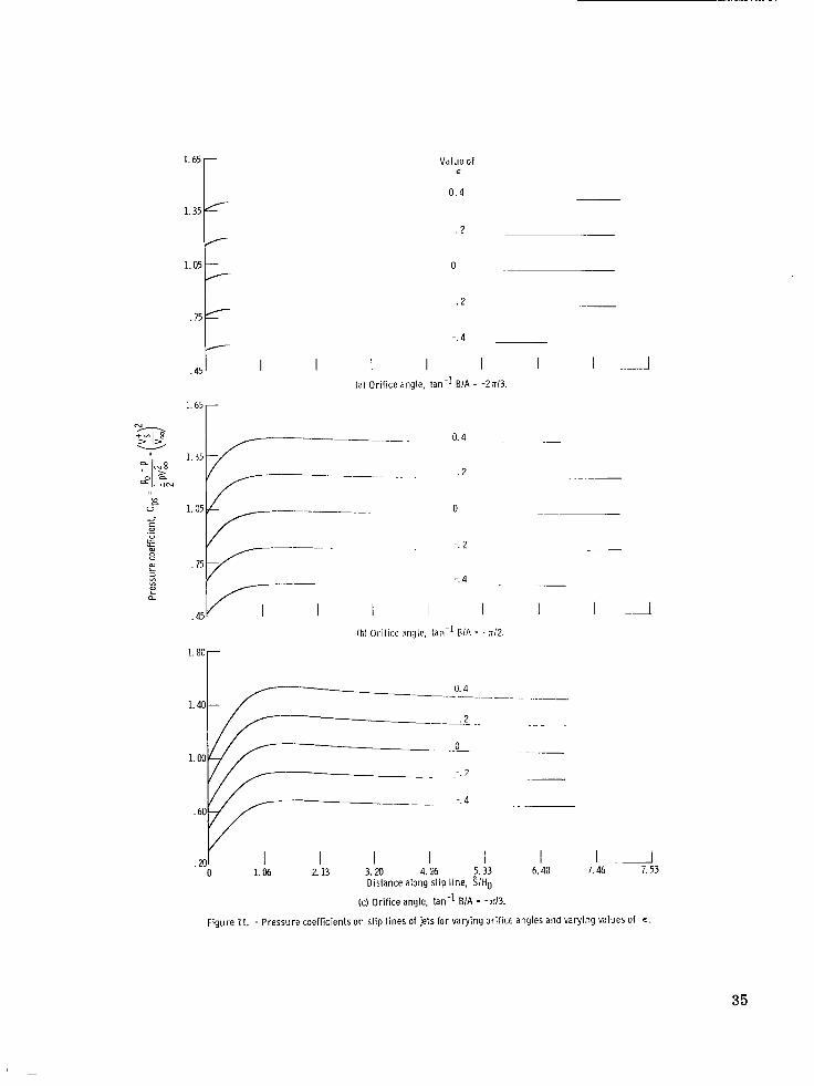
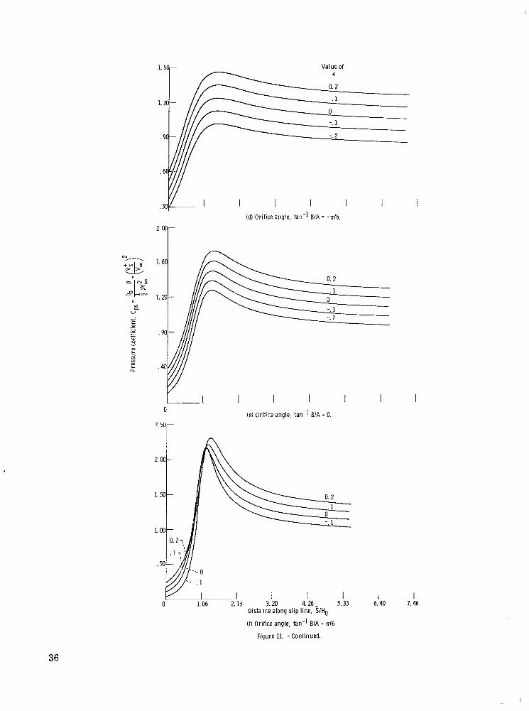
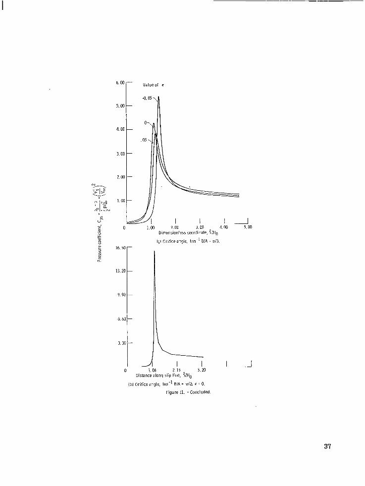
The pressure coefficient on the slip line is obtained as a function of the distance along the slip line in parametric form from equations (61) and (65) after using definitions (521, (54), (569, and (58). The results of these calculations are shown in figures ll(a) t o (h). Each figure is dmwn for a different orifice angle. These curves contain all the information necessary for calculating the viscous boundary layer along the sl ip line. The curves show that for a fixed orifice angle the velocity at both the upstream edge of the orifice and at the downstream end of the sl ip line increases with increasing E.

negative orifice angles the velocity tends to be relatively constant along the slip line, ex- hibiting a slight dip at the upstream edge of the orifice. A s the orifice angle is increased toward zero the variation of velocity along the slip l-he becomes more pronounced. nonnegative values of the orifice angle there is a definite peak in the velocity profiles which beconies more marked as the orifice angle is increased. This peak is attributed to the fact that the velocity is infinite at the downstream edge of the orifice. Since this point moves closer to the slip line as the orifice angle is increased, the velocity along the slip line becomes more peaked as the orifice angle increases. the velocities (pressure coefficients) on the slip lines of the attached and separated jets is illustrated in figure 12 for zero orifice angle. The pressure coefficient of the separated jet rises monotonically to l far downstream. This smoother behavior can be attributed to the presence of the wake which adjusts in shape to keep the velocity of the turning jet f rom getting too large and the pressure from dropping too far below the static pressure of the stream. If the downstream wall is actually very thin, viscous effects will very likely cause the formation of a separation bubble at the lip. In that event, the velocity distribution on the slip line will'fall between the two extremes shown in the figure.

Figures lO(a) and (f) show that, as in the

For

For

The contrast between

32

1. l o r

Value of E

0.2 7,

. 1 y.',

0 I > .

(a) Ori f ice angle, tan-1 B / R = 0.

-1. -.401 uo I 7"1 I c r I I I t , I I I I I r I i I I I TJ I I I I I I I t I I I I I I I I I I I I 1 I I I I I I I I , I I I I I r I 1 I I I I

(b) Or i f i ce angle, tan'' B/k = - 2 d 3 . Abso!uie va lue of epsilon, I E 15 0.4.

-. -f 40

Dimensionless coordinate, XlHo

( ~ l ) Or i f i ce angle, t a n - 1 B ~ A = ~ / 3 .

Figure 10. - Jet c o n t o u r s for vary ing o r i f i c e angles a n d vary ing values o f e .

33

e

Value o f

0. 2 7 , E

-_ 10 - 1T .50

1 1 1 1 1 1 I I I I I I I I I I , , , , , , , , , , , , , , , , I I I I T I I I I I (e) Or i f i ce angle, t a n - l B I 4 = -7d6.

0. 2 7 , .17'\

1

I It.

\ \

0 7, '\ \\ \ \ -. 1 :> \, ',

I I I I I (f) Or i f i ce angle, tan- ' BIA = 7rI6.

0.05 T,

-.OS\, '\

0 -, '\\

___ \ '\ '\

( g ) Or i f i ce angle, t a n - 1 BIA = n/3.

I I I I I I I ( h ) Or i f i ce angle, tan-' BIA = d 2 ; E = 0.

~~ . . . . . . , . , , , , . . . . . -, . , -.

--. 10

1. 10

-. 10 1 I 1 -2.00 -1.40 -.SO -. 20 .40 1.00 1.60 2.20 2.80 3.40 4.00

Dimensionless coordinate, XIHO

( i ) Or i f i ce angle, tan- ' BIA = 2 d 3 ; E = 0.

F igure 10. - Concluded.

34

1.65

.45

Value of

0 .4

E

. 2

~~ 0

-. 2

-. 4

I I I I I II (a1 Orifice angle, tan-' B/A = - 2 d 3 .

i'65r 0.4 _ ~ ~ _ _ _

1.35

_~ . 2

~~ ~

1.05E::-: .75 - _ _ ~ . -' 0 -. -. 4 2 _- -

.45 I I I I -_I

(bl Orifice angle, tan" B/A = -n /2 .

.201 I 0 1.06

II 7.46 7. 53

I 6.40

I 5.33

I 4.26

Distance along slip line, S / H ~ (c) Orif ice angle, tan-1 BIA = -r/3.

Figure 11. - Pressure coefficients on slip l ines of jets for varying orif ice angles and varying values of E .

I 3.20

I 2. 13

35

1 . 5 L t Value of E

0.2

1. a- 0

I I I I (d) Orifice angle, t an - l B/A = -71/6.

1 . 6 0 1

1 I

I I I I (e) Orifice angle, tan-1 BIA = 0.

0 I I

1 6.40

I 7.46

( f l Grifice angle, tan-’ BIA = 7r/6

Figure 11. -Continued.

36

b. 00

5.00

4.00

3.00

Valueof E

4.05 -

O-\\

.os-, I

.1 I I I 1 c 1.00 2. co 3. on 4. 00 sl00 u Dimensionless coordinate, ?/Hn a,

0 .- .- ”-. L

m 0 (g) Orif ice angle, tan-’ BIA = 7 d 3 . E

E YI

a

L I I 1

3. 20

(h) Orif ice angle, tan-’ B/A = d 2 ; E = 0.

I 0 1.06 2.13

Distance along slip line, S/HO

A

Figure 11. - Concluded.

37

I 12

~~ I 10

I 8

I 6

I 2 4

Distance along jet boundary, 5lH

Figure 12. - Pressure coefficients o f attached and separated jets. Orifice angle, tan-1 BIA = 0; E = 0.

CONCLUDING REMARKS

A procedure developed in reference 1 has been applied to obtain a solution to the problem of a two-dimensional inviscid jet injected from an orifice at an oblique angle to a moving s t r eam for the case where the jet does not separate from the downstream edge of the orifice. The analysis shows a peaking of the pressure coefficient along the slip line which increases as the orifice is tilted into the s t ream. s t ream also makes the jet contraction ratio more sensitive to changes in total pressure in the jet.

Tilting the jet into the

Lewis Research Center, National Aeronautics and Space Administration,

Cleveland, Ohio, August 12, 1969, 129-01.

38

REFERENCES

1. Goldstein, M. E. ; and Braun, W. : Tnjection of an Inviscid Separated Jet at an Oblique Angle to a Moving Stream. NASA T N D-5460, 1969.

2. Batchelor, G. K. : An Introduction to Fluid Dynamics. Cambridge University P res s , 1967, pp. 410-412.

3. Birkhoff, Garrett; and Zarantonello, E. H. : Jets, Wakes, and Cavities. Academic Press, 1957.

4. Ehrich, Fredric F. : Penetration and Deflection of Jets Oblique to a General Stream J. Aeron. Sci., vol. 20, no. 2, Feb. 1953, pp. 99-104.

5. Churchill, Rue1 V. : Complex Variables and Applications. Second ed. , McGraw-Hi1 Book Co., Inc., 1960.

6. Muskhelishvili, Nikolai I. : Singular Integral Equations. P. Noordhoff, Ltd. , 1953. "

NASA-LanSley, 1969 - 12 E-5106

I - ~~

39

NATIONAL AERONAUTICS AND SPACE ADMINISTRATION WASHINGTON, D. C. 2054G

OFFICIAL BUSINESS FIRST CLASS MAIL =- POSTAGE A N D FEES PA1

SPACE ADMINISTRATIOi' NATIONAL AERONAUTICS

"The nesonantical and space activities of the United Stntes shnll be condxcted so a~ to contribute . , . t o the expnnsion of human knoiul- edge of phenoniena in the atmosphese and space. The Administsntioa shall psovide for the widest practicable and nppropsiate disseminatioiz of iaf osni~ztion concerning its activities nnd the results thereof."

-NATIONAL AERONAUTICS A N D SPACE ACT OF 1953

NASA SCIENTIFIC AND TECHNICAL PUBLICATIONS

TECHNICAL REPORTS: Scientific and technical information considered important, complete, and a lasting contribution to existing knowledge.

TECHNICAL NOTES: Information less broad in scope but nevertheless of importance as a contribution to existing knowledge.

TECHNICAL MEMORANDUMS : Information receiving limited distribution because of preliminary data, security classifica- tion, or other reasons.

TECHNICAL TRANSLATIONS: Information published in a foreign language considered to merit NASA distribution in English.

SPECIAL PUBLICATIONS: Information derived from or of value to NASA activicies. Publications include conference proceedings, monographs, data compilations, handbooks, sourcebooks, and special bibliographies.

TECHNOLOGY UTILIZATION PUBLICATIONS: Information on technology used by NASA that may be of particular interest in commercial and other non-aerospace npp!ications. Publications include Tech Briefs, T ~ c h n o ~ o ~ g y Utilization Reports and Notes, and Technology Surveys.

CONTRACTOR REPORTS: Scientific and technical information generated under a NASA contract or grant and considered an important contribution to existing knowledge.

Details on the availability of fhese publications may be obtained from:

SCIENTIFIC AND TECHNICAL INFORMATION DIVISION

NATIONAL AERO N AUTICS AND SPACE ADM I N I STRATI0 N Washington, D.C. 20546

nasa technical note nasa tj · nasa technical note nasa tj d-5501 0. / f ... ohio 441 35 9. ... cid...

Documents