Multiple Pulses in dE/dt and the Fine-Structure of E During the Onset of First Return Strokes in Cloud-to-Ocean Lightning

Natalie D. Murray, E. Philip Krider, and John C. Willett

Institute of Atmospheric Physics

The University of Arizona Tucson, Arizona 85721-0081

U.S.A.

Revised 11 August 2004

Abstract

We have analyzed the fine-structure of 131 electric field (E) waveforms that were

radiated during the onset of first return strokes in cloud-to-ocean lightning. The

dE/dt waveforms were recorded using an 8-bit waveform digitizer sampling at

100 MHz, and the E waveforms were sampled at 10 MHz using a 10-bit digitizer.

49 (or 37%) of the dE/dt waveforms contain one or more large pulses within

±1 µs of the largest (or dominant) peak in dE/dt, i.e. within an interval from -1 µs

to +1µs, where t = 0 µs is the time of the dominant peak, and 37 (or 28%) have

one or more large pulses in the interval from 4 µs before to 1 µs before the

dominant peak, i.e. -4 µs to –1 µs, and only the dominant peak within ± 1 µs .

We give statistics on the amplitude and timing of dE/dt pulses that are near the

dominant peak, and we show how the presence of these pulses adds

considerable fine-structure to the shape of Eint, the integrated dE/dt waveform, on

a time-scale of tens to hundreds of nanoseconds. This fine-structure includes

fast pulses near the beginning of the slow front, large pulses and shoulders

within the slow front and during the fast transition, and very narrow peaks in Eint.

Our overall conclusion is that the electromagnetic environment near the point(s)

where lightning leaders attach to the surface is often more complicated than what

would be produced by a single current pulse propagating up a single channel at

the time of onset.

2

1.0 INTRODUCTION

Submicrosecond measurements of the electric field, E, and dE/dt waveforms that

are radiated during the onset of first return strokes in cloud-to-ocean lightning

have been reported previously by Weidman and Krider (1978; 1980; 1984),

Krider et al. (1996), Willett et al. (1995; 1998), and Willett and Krider (2000).

Weidman and Krider (1978; 1980) noted that the shape of the initial E field, when

recorded under conditions where there is minimal distortion due to the effects of

ground-wave propagation, typically begins with a slow, concave front that lasts

for several microseconds. The front is followed by a fast-transition to the peak E,

and then there are a variety of subsidiary peaks and other features that are

thought to be due to the effects of branches, the complex geometry of the

channel, and/or traveling waves of current during the attachment process

(Weidman and Krider, 1978; Weidman et al., 1986; Willett et al., 1988;

Leteinturier et al., 1990). In the discussion of their Fig. 2c to 2f, Weidman and

Krider (1978) noted that sometimes the slow front has a convex shape, rather

than concave, and they hypothesized that this might be due to the impulse from a

leader step being superimposed on the initial rise of the return stroke field.

Willett and Krider (2000) reported that 39% of their first stroke waveforms had

multiple pulses in dE/dt near the time of the fast-transition in E (see their Fig. 3),

and they noted that E waveforms obtained by numerically integrating their dE/dt

records (100 MHz sampling) sometimes contained very narrow, fast peaks not

resolved by an E waveform digitizer sampling at 10 MHz. Given the above and

3

the relative paucity of waveform measurements on natural lightning with very fast

time-resolution, we have re-examined the fine-structure of the dE/dt and E

waveforms in the dataset described by Willett et al. (1998) and Willett and Krider

(2000) with the goal of quantifying this structure on a time-scale of tens to

hundreds of nanoseconds.

2.0 DATA

Our database comprises 131 dE/dt and E waveforms that were recorded in 1985

just north of the NASA Kennedy Space Center (KSC) on Playalinda Beach,

Florida (Willett et al., 1998). The lightning locations were measured using a

network of three gated, wideband magnetic direction-finders (Krider et al., 1980)

that provided an overall location accuracy of about 1 km (Maier and Jafferis

1985; Krider et al. 1996). The flashes occured at ranges of 5 to 50 km on three

thunderstorm days, and maps showing the locations of the experiment site and

the lightning strike points are given in Willett et al. (1990, Fig. 2) and Willett et al.

(1998, Figs. A2, A3, and A4). Three independent flush plate antennas mounted

on the roof of a well-grounded metal trailer were used to measure the E, dE/dt,

and RF signals produced by the lightning. The trailer housed the recording

electronics and was parked about 45 m from the Atlantic Ocean so that any fields

originating from lightning over the ocean would be measured with minimal

distortions due to the effects of propagation over the ocean/land surface (Cooray

and Ming, 1994; Cooray, 2003, Chapter 7; Cooray et al., 2004).

Indeed, Krider et al. (1996) have previously argued that E and dE/dt

measurements made at a similar site in 1984 were not significantly affected by

4

propagation. Willett et al. (1998, Table 1) also showed that the mean peak dE/dt

in 1985 was comparable to that in 1984, and that the full-width-at-half-maximum

(FWHM) of the initial half-cycle of dE/dt in 1985 had a mean that was comparable

to, or possibly even slightly less, than that in 1984. Because the waveform

measurements in 1985 were at comparable ranges to those in 1984 and

produced similar results, we believe that there are minimal distortions in the 1985

waveforms due to the effects of propagation. This issue will be examined further

in section 5.5.

A block schematic diagram of the data acquisition system has been given by

Willett et al. (1989, Fig. 1). dE/dt waveforms were digitized using an 8-bit A/D

converter sampling at 100 MHz, and E waveforms were digitized using a 10-bit

A/D converter sampling at 10 MHz. The effective bandwidths of the dE/dt and E

recording systems were about 30 MHz and 3 MHz, respectively. Both digitizers

were triggered on the output of a wideband RF receiver tuned to 5 MHz in order

to minimize any biases that might be introduced by the finite trigger threshold.

Krider et al. (1996) and Willett et al. (1998) have given detailed discussions of the

possible trigger biases in 1984 and 1985, respectively. No evidence has been

found for a range-dependence in the values of the range-normalized peak dE/dt,

and there is no indication that the values of FWHM have been biased by the RF

triggering technique.

Plots of all dE/dt and E waveforms in our dataset, together with the outputs of the

RF receiver and the slow-E antenna, are given in technical reports by Bailey and

5

Willett (1989) and Izumi and Willett (1991). The type of lightning process that

triggered the recording system was determined from the overall shape and

structure of the E and slow-E waveforms. All CG flashes in our dataset

effectively lowered negative charge toward ground, and the initial E fields were

negative or downward transitions following the physics sign convention. The

amplitudes of all waveforms given in this paper have been range-normalized to

100 km, assuming that the radiated field has an inverse-distance dependence on

range and that any attenuation of high frequencies by propagation over the

ocean surface and the narrow strip of land is negligible.

3.0 CHARACTERISTICS OF dE/dt AND E WAVEFORMS

The primary focus of this paper will be on a 5 µs interval that corresponds to the

onset of first stroke waveforms, i.e. the slow front, the fast-transition, and the

initial peak of E. We start by examining the number and timing of large pulses

that appear in the dE/dt records, and we then consider the effects that these

pulses have on the fine-structure of E. Any deviations from the normal or

“classical” shapes (e.g., Weidman and Krider, 1978) will be noted and further

classifications will be assigned as necessary.

To determine the fine-structure of E, each dE/dt record (100 MHz) has been

numerically integrated over a 15 µs interval that includes the peak E to provide a

waveform that we designate Eint. This integration has been done using the

trapezoidal rule, and because the shape of Eint is very sensitive to small offsets in

6

dE/dt, we systematically stepped through a number of offsets and then selected

the one that provided the best least-squares fit to the measured 10 MHz E

waveform. (The results of this procedure are shown in red in Fig. 1b, 2b, and 4

through 13 to follow and will be discussed in detail below.) In order to keep the

effects of any residual baseline offsets from affecting the values of peak Eint

(given in Table 1 and Fig. 14 to follow), we also averaged Eint over the first 5 µs

of the 15 µs integrating interval (typically including only a few leader steps) and

then subtracted this average from the value of the peak Eint. Additionally,

because the time differentiation inherent in a dE/dt recording causes any

information about the variations in E below some frequency to fall below the

lowest level of digitizer resolution, Eint occasionally exhibits spurious low-

frequency features that do not match the (correct) behavior that is preserved in

the 10 MHz E record (e.g., Fig. 4). Because of this, we also visually compared

the offset of Eint at – 4 µs (the origin of our time-scale will be discussed in section

3.2) with the corresponding 10 MHz E record and subtracted the difference from

the value of the peak Eint. (One example of this zero level correction is illustrated

by the horizontal green line in Fig. 4 to follow.)

3.1 Single Peak dE/dt Waveforms (Type A)

Fig. 1a shows the initial portion of a “classical” E waveform from a first return

stroke together with the corresponding dE/dt signature. Events like this, which

produce a single large pulse in dE/dt corresponding to the fast-transition in E, will

be termed “Type A” strokes. The same waveform as in Fig. 1a is shown on an

expanded time scale in Fig. 1b. Here Eint signature has been plotted in red

7

together with the individual samples of E (asterisks). Our term “pulse in dE/dt”

usually refers to an isolated negative impulse that is immediately followed by a

positive overshoot, as shown in the upper panel of Fig. 1b. We define the

“dominant peak” in dE/dt to be the largest negative-going pulse that occurs

during the fast-transition in E. Note that, in Fig. 1b, how the origin of the time-

axis has been shifted to coincide with the time of the dominant peak.

3.2 Multiple Peak dE/dt Waveforms

Fig. 2 shows records similar to Fig. 1, but for a stroke that produced multiple

pulses in dE/dt near the time of the peak E. Since multiple pulses were present

in a significant fraction of our dE/dt records, we will now examine the

characteristics of these features in more detail.

In order to classify the dE/dt waveforms, we counted pulses if they had: (a) a

(negative) peak amplitude that was at least 10% of the amplitude of the largest or

dominant peak and (b) the (positive-going) return of that signal toward the

baseline reached a (negative) level that was 50% of its own (negative) peak

amplitude. Strokes that had multiple pulses in dE/dt were further classified

according to the time of any additional pulse (or pulses) relative to the dominant

peak. Here we will focus primarily on pulses that occur in the 5 µs interval from -

4 µs to +1 µs, i.e., 4 µs before to 1 µs after the dominant peak, and we will

assume that all pulses prior to –4 µs, a typical duration of the slow front

(Weidman and Krider, 1978; 1980), were produced by the final steps of the

stepped-leader process that initiated the stroke rather than by the onset of the

8

stroke itself (Krider et al., 1977). Of course, some of the pulses which occurred

after -4 µs could be due to leader steps, and we will consider this point further in

section 3.3.

Fig. 3 summarizes the characteristics of all dE/dt pulses that satisfied the above

selection criteria and that occurred in a 10 µs interval containing the dominant

peak (i.e. –9 µs to +1 µs). Fig. 3a gives the number of pulses (excluding the

dominant peak) in consecutive one microsecond time bins, and Fig. 3b shows

the mean (negative) amplitude of these pulses relative to that of the dominant

peak. Fig. 3c shows an example of the types of pulses that were included in Fig.

3a and 3b.

Within our total sample of 131 first return strokes, each having a dominant peak,

49 (or 37%) produced one or more pulses in dE/dt (in addition to the dominant

peak) within ± 1 µs of the dominant peak, and these events will be termed “Type

B” strokes. 37 (or 28%) of first strokes produced one or more pulses in the

interval from –4 µs to – 1 µs before the dominant peak (and no pulse within

± 1 µs of the dominant peak). These events will be termed “Type C” strokes.

Thus, there are a total of 86 first strokes – an astonishing 66% of the total – that

produced multiple pulses in dE/dt in a 5 µs interval near the dominant peak in

dE/dt (and the peak E). (Although not directly noted above, all first stroke

waveforms in our dataset had considerable fine-structure after the initial peak E,

i.e., α-peaks and other subsidiary features termed a, b, c by Weidman and Krider

(1978; 1980).)

9

3.2.1 Type B Events

The 49 Type B events produced a total of 136 large pulses in dE/dt (in addition to

the dominant peak) within ± 1 µs of the dominant peak; therefore, the average

number of pulses between -1 µs and 1 µs in Type B strokes was (136+49)/49 or

3.8, including the dominant peak. It should be noted that the average amplitude

of the extra pulses in Type B strokes was about 40% of the dominant peak (see

Fig. 3b). Fig. 2 and 4 to 7 to follow show examples of the dE/dt and Eint

waveforms produced by Type B strokes.

3.2.2 Type C Events

The 37 events classified as Type C strokes produced a total of 85 pulses in dE/dt

in the interval between –4 µs to –1 µs relative to the dominant peak and no

additional pulses in the interval from ±1 µs except the dominant peak. Thus the

average number of dE/dt pulses in Type C strokes was (85+37)/37 or 3.3,

including the dominant peak. (Note: some of the Type B strokes also had pulses

between –4 µs and –1 µs, and although such pulses are not counted here, they

are counted in Fig. 3.) Fig. 8 to 12 give examples of the dE/dt and Eint waveforms

produced by Type C strokes.

10

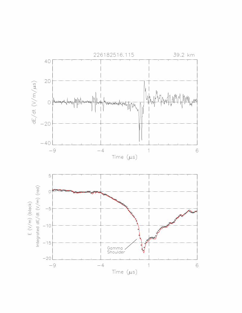
3.3 Leader Step Waveforms

Practically all events in our dataset showed evidence of E and dE/dt radiation

from the final steps of the stepped-leader process that preceded the onset of the

first return stroke. The shapes of the leader dE/dt pulses tend to fall into two

broad categories: (a) a single large impulse, which we term a “leader step” or LS

waveform and (b) a short burst of smaller pulses which we term a “leader burst”

or LB signature. The integral of both types of dE/dt waveforms produces an

almost unipolar E signature with a duration of about one microsecond. (See

Krider et al.,1977, and Willett and Krider, 2000, for further discussions of leader

step waveforms.) In our total sample of 131 first stroke waveforms, 48 (or 37%)

had an LS impulse in the 5 µs interval from -9 µs to -4 µs before the dominant

peak, and 75 (or 57%) had a LB in that interval. Many examples of LS and LB

waveforms can be seen in Fig. 2 to 13, and specific examples have been labeled

in Fig. 2b, 8, 9, 11 and 13. As we will see, many of the waveforms that contain

multiple pulses in dE/dt between -4 µs and 1µs could be the result of large LS

and/or LB waveform(s) being superimposed on the onset of the return stroke

field. Further details about the characteristics of LS and LB waveforms will be

given in a future paper.

4.0 FINE-STRUCTURE OF THE EINT WAVEFORMS

We have seen that the dE/dt signatures radiated during the onset of first return

strokes can be broadly classified into: Type A events that have a single, negative

(dominant) peak in a 5 µs interval that contains the peak E; Type B events that

have one or more additional pulses within ±1 µs of the dominant peak; or Type C

11

events that have a dominant peak and at least one additional pulse in the interval

from –4 µs to –1 µs, and no additional pulses within ± 1 µs of the dominant peak.

The shapes of the corresponding Eint waveforms have reproducible features that

depend upon the amplitude and timing of the dE/dt pulses relative to the

dominant peak.

4.1 Type A Events

Strokes with a single, dominant peak in dE/dt tend to produce the “classical” Eint

waveform as described by Weidman and Krider (1978), i.e., a slow, concave

front followed by a fast-transition to peak, and little additional structure. The Eint

waveforms in Fig. 1 and Fig. 13 are typical Type A signatures.

4.2 Type B Events

The Eint waveforms for Type B strokes tend to have an inflection point (or

shoulder) within or near the fast (negative-going) transition in Eint or, if the

additional dE/dt pulse contains a (positive-going) zero crossing, there are

multiple peaks in Eint. We term any such peaks or shoulders “γ-peaks” or “γ-

shoulders,” and, of course, such features can occur either near the beginning, in

the middle (Fig. 4), or toward the end (Fig. 5) of the fast-transition, depending on

the relative amplitude and timing of the pulses in dE/dt. Fig. 6 shows two well-

defined γ-peaks that are very narrow (less than 0.2 µs). Here, the effect of

multiple pulses in dE/dt is to produce a 0.5 µs delay between the dominant peak

(in dE/dt) and the peak Eint. Of the 49 Type B strokes in our dataset, 31

produced a total of 34 γ-peaks, and all except one had one or more γ-shoulders.

The waveform shown in Fig. 9 (discussed further below) has a feature similar to

12

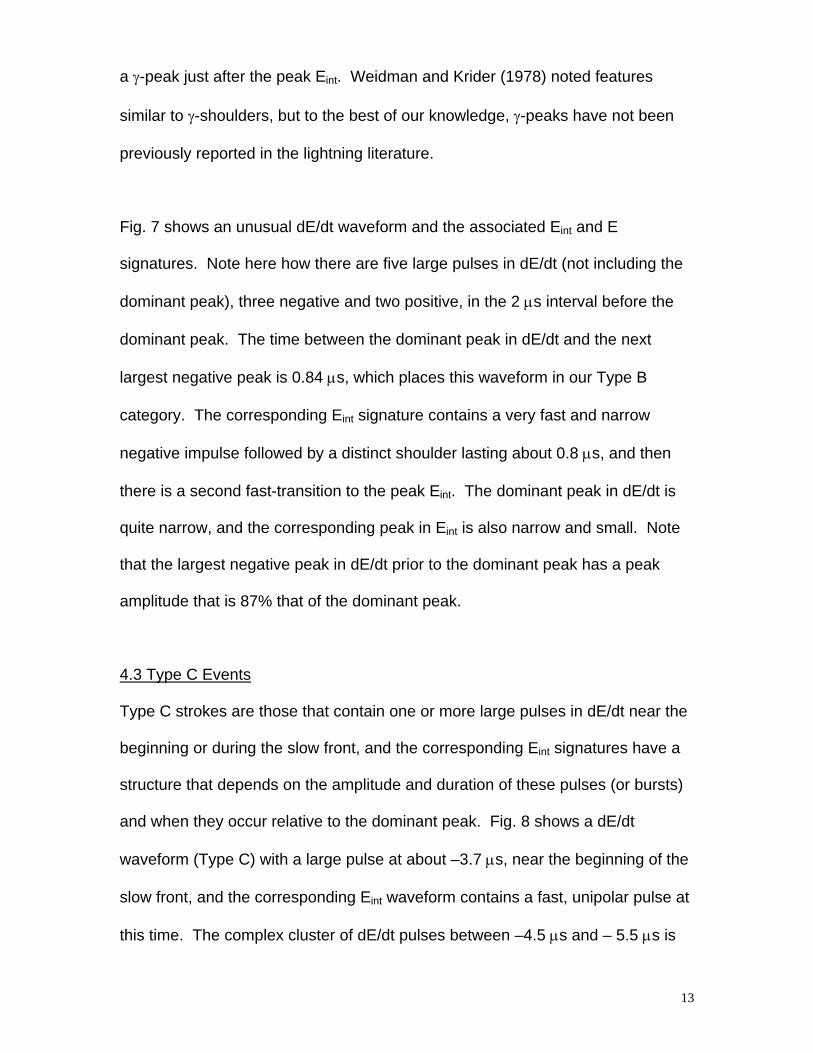
a γ-peak just after the peak Eint. Weidman and Krider (1978) noted features

similar to γ-shoulders, but to the best of our knowledge, γ-peaks have not been

previously reported in the lightning literature.

Fig. 7 shows an unusual dE/dt waveform and the associated Eint and E

signatures. Note here how there are five large pulses in dE/dt (not including the

dominant peak), three negative and two positive, in the 2 µs interval before the

dominant peak. The time between the dominant peak in dE/dt and the next

largest negative peak is 0.84 µs, which places this waveform in our Type B

category. The corresponding Eint signature contains a very fast and narrow

negative impulse followed by a distinct shoulder lasting about 0.8 µs, and then

there is a second fast-transition to the peak Eint. The dominant peak in dE/dt is

quite narrow, and the corresponding peak in Eint is also narrow and small. Note

that the largest negative peak in dE/dt prior to the dominant peak has a peak

amplitude that is 87% that of the dominant peak.

4.3 Type C Events

Type C strokes are those that contain one or more large pulses in dE/dt near the

beginning or during the slow front, and the corresponding Eint signatures have a

structure that depends on the amplitude and duration of these pulses (or bursts)

and when they occur relative to the dominant peak. Fig. 8 shows a dE/dt

waveform (Type C) with a large pulse at about –3.7 µs, near the beginning of the

slow front, and the corresponding Eint waveform contains a fast, unipolar pulse at

this time. The complex cluster of dE/dt pulses between –4.5 µs and – 5.5 µs is

13

what we are terming a “leader burst,” and note how the corresponding Eint

waveform is almost unipolar. There were 15 waveforms of the type shown in Fig.

8 in our dataset.

Four strokes produced large pulses in dE/dt during the development of the slow

front, and these tended to produce Eint waveforms like that shown in Fig. 9. Two

strokes produced bursts of dE/dt pulses during the slow front, and the

corresponding front in Eint was convex as shown in Fig. 10. Seven strokes

produced multiple pulses in dE/dt during the front, and Fig. 11 shows how such

pulses create an abrupt negative transition or a shoulder in Eint that is followed by

a slower, clearly defined plateau prior to the fast-transition. Fig. 12 shows how a

burst of 3 dE/dt pulses at - 2 µs created an abrupt shoulder in Eint.

5.0 DISCUSSION

5.1 Narrow Peaks in Eint Fig. 13 shows an example of an Eint waveform that has a very narrow peak which

was not resolved by the 10 MHz E digitizer (see also Fig. 2b, 4, 7 and 8). Since

narrow peaks were a fairly common feature in our data set, and since the values

of peak E are often used to infer the peak current in first return strokes (Rakov

and Uman, 1998; Cummins et al., 1998a,b), we have compared the values of

peak Eint, obtained by integrating dE/dt waveforms (100 MHz sampling), with the

values of peak E obtained from the 10 MHz E digitizing system. Table 1 and Fig.

14 summarize the results for all Type A, B, and C strokes in our dataset. Note in

14

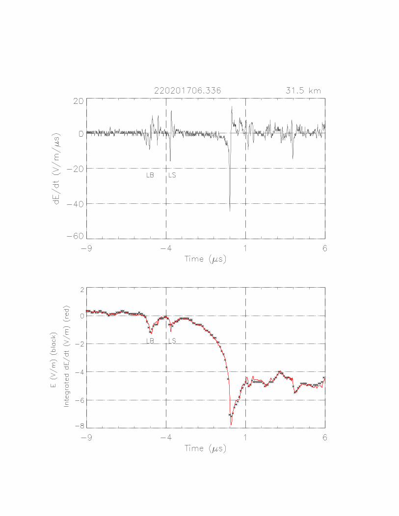
Fig. 14 that 13 strokes (10% of the total) have a peak Eint/peak E ratio equal to or

greater than 1.15, the maximum is 1.31, and the mean is 1.07. The values of the

peak Eint and peak E (range-normalized to 100 km) in Table 1 have an overall

mean and standard deviation (SD) of -9.0 ± 4.4 V/m and -8.6 ± 4.4 V/m,

respectively, and the median peak Eint and peak E are –7.9 V/m and -7.2 V/m,

respectively. It should also be noted in Table 1 that the integrated effect of

multiple peaks in dE/dt (Type B strokes) is to produce a mean amplitude that is

about 40% larger than that of the single-peak (Type A) strokes.

To quantify the width of the fast peaks in Eint, we have measured the time-interval

between the dominant (negative) peak in dE/dt and the peak of the (positive)

overshoot that immediately follows the dominant peak in 114 events where the

dominant peak corresponded to the fast-transition in Eint and where the positive

overshoot in dE/dt had a well-defined peak (see, for example, Fig. 13) and

events like those shown in Fig. 5 and 6 were omitted. The results are shown in

Fig. 15. Note that the intervals in Fig. 15 range from 0.04 µs to 0.26 µs (with a

digitizer resolution of 0.01 µs). The mean and SD are 0.11 ± 0.04 µs, and the

median is 0.10 µs. 70 (or 60%) of the 114 strokes in Fig. 15 had an interval (as

defined above) that was less than 0.12 µs; therefore, any digitizing system that

samples E at a frequency of 10 MHz or less (i.e., a sampling interval of 0.1 µs or

greater) will not be capable of resolving the true peak field or the other fine-

structure that is often present in E during the onset of first strokes.

15

Fig. 16 shows the amplitude of the positive overshoot in dE/dt relative to the

dominant (negative) peak for the 114 strokes that have been plotted in Fig. 15.

The mean and SD of these ratios are 0.27 ± 0.16, the median is 0.26, and 86%

of the overshoot amplitudes are less than 40% of the dominant peak.

One possible explanation for the very narrow peaks in Eint has been suggested

by Leteinturier et al. (1990); namely, if the first return stroke begins at an

elevated junction point between the upward connecting discharge and the last

step of the downward-propagating stepped-leader, traveling waves of current

might propagate both upward and downward from this point until the downward

wave is partially reflected at the surface. During the time when there are both

upward and downward propagating waves, the radiated field could be up to a

factor of two larger than what would be radiated after the partial reflection (see,

for example, Fig. 17 in Leteinturier et al. (1990) and the discussion in Cooray et

al. (2004)).

5.2 Peak E vs. Peak dE/dt

Fig. 17 shows plots of the peak Eint vs. the (dominant) peak dE/dt for all Type A,

B, and C strokes in our dataset. Note that the values for the Type A and Type C

strokes are moderately well correlated (R2 values of 0.501 and 0.503,

respectively) but with different slopes. Type B strokes have little correlation (R2 =

0.013), presumably because the peak Eint is dominated by the integrated effects

of the multiple pulses in dE/dt. The slope of the Type A fit is similar to, but not

directly comparable with, that of Willett and Krider (2000, Fig.5), who excluded all

16

Type B waveforms and some Type C waveforms from their analyses and then

compared the peak dE/dt to the amplitude of the fast-transition in E (i.e., the slow

front was omitted). The slopes of the regression lines in Fig. 17 have units of

time and can be regarded as a characteristic rise-time of Eint. This interpretation

is only valid for the Type A events, however, where a single pulse in dE/dt is

uniquely associated with the fast-transition in Eint. For the 45 Type A events, this

characteristic rise time is about 160 ns which is about twice the 83 ns obtained

by Willett and Krider (2000, Fig. 5), who plotted just the amplitude of the fast-

transition (which they termed Ef) as a function of the peak dE/dt for 76 first

strokes in the same dataset with “single dE/dt peaks during the fast-rising

portion” (roughly our Type A and Type C). (Willett and Krider (2000) also found

that the slow front in those 76 events represented about 50% of the total

amplitude of E.)

5.3 Energy Spectral Density of dE/dt

Willett et al. (1990, Appendix A and Fig. A1) have described a method for

computing the energy spectral density (ESD) of the early portion of return stroke

fields from recorded dE/dt signatures. We have used the same method to

compare the ESD of 45 Type A and 49 Type B waveforms over a 15 µs interval

that includes the onset of the return stroke and peak E (-9 µs to +6 µs). The

results are shown in Fig. 18. Note how the presence of multiple peaks near the

fast-transition in E (Type B) enhances the average ESD relative to a single,

dominant peak (Type A) above about 5 MHz, and it also produces a relative

minimum between 2 and 4 MHz. The mean time-interval between the two largest

17

negative peaks in dE/dt (in the –1 µs to +1 µs interval) in the 49 Type B strokes

was 0.31 ± 0.2 µs, and the median was 0.24 µs; the minimum in the spectrum is

consistent with this spacing.

5.4 Subsequent Return Strokes

We have examined the dE/dt waveforms produced by the subsequent return

strokes in our dataset, i.e., the strokes that come after the first in a flash and that

do not appear to initiate new attachments to ground (e.g., Willett et al.,1995), to

see if there were multiple pulses in dE/dt during the onset of those strokes. The

results are summarized in Table 2 together with our results for the Type A and

Type B first strokes. Table 2 shows that a substantial fraction of the subsequent

strokes in natural lightning do produce multiple peaks in dE/dt within ± 1 µs of the

dominant peak, and that the subsequent strokes preceded by dart-stepped

leaders have a greater fraction of multiple peaks in this interval than the first

strokes (66 % vs. 37%). Leteinturier et al. (1990, Fig. 5) and Uman et al. (2000,

Fig. 4) give examples of multiple pulses in dE/dt during the onset of subsequent

strokes in rocket-triggered lightning. In the future, we plan to analyze the fine-

structure of the Eint waveforms produced by subsequent strokes in more detail.

5.5 Propagation

As we have seen, the dE/dt and Eint waveforms radiated by the first return

strokes in cloud-to-ocean lightning frequently contain large variations on a time-

scale of tens to hundreds of nanoseconds. The waveforms were recorded at

ranges of 4 to 40 km and, as we stated in section 2.0, they have not been

18

corrected for the effects of ground-wave propagation because the propagation

paths were almost entirely over ocean water. Krider et al. (1996) have estimated

that propagation over a smooth ocean surface will reduce the peak dE/dt and

increase the full-width-at-half-maximum (of the negative half-cycle) by about 6%

and 11%, respectively, at a range of 10 km, and by 15% and 33%, respectively,

at a range of 35 km (see their Table 2). In order to evaluate whether such effects

might be present in our dataset, Fig. 19 and 20 show the values of peak dE/dt

(range-normalized to 100 km) and the effective width of the sharp peaks in Eint,

i.e., the time-interval between the dominant negative peak in dE/dt and the peak

of the positive overshoot that immediately follows the dominant peak (as in Fig.

15), as a function of range, respectively. Since neither of these Fig. shows any

significant range-dependence, we believe that the effects of propagation in this

dataset are minimal.

5.6 Physical Interpretation

If there are large variations in dE/dt and E on a time-scale of tens to hundreds of

nanoseconds during the onset of first return strokes, then there must also be

comparable variations (but perhaps not a strict proportionality) in the channel

current, I, and dI/dt at or close to the point(s) where lightning leaders attach to

the surface and the electric fields are produced. Large values of dI/dt will be

produced whenever there is an abrupt onset (or termination) of any large current

that flows during the breakdown of air, in response to a large potential difference.

Possible causes include multiple pulses of current in a single channel, such as

might be present if the development of the last step of the downward-propagating

19

leader or the upward-propagating connecting discharge develops in an

intermittent fashion, or if there are large reflections of traveling waves of current

during the attachment process. It is also possible that there are multiple

channels, perhaps due to branches or forks in the last leader step and/or the

upward connecting discharge, or that loops or forks form at the time of

attachment. In any case, our results clearly show that the electromagnetic

environment near the point(s) where lightning leaders attach to the surface is

often more complicated than what would be produced by a single current pulse

propagating up a single channel at the time of onset. (see, for example, Rakov

and Uman, 1998; 2003, Chapter 12; and Cooray et al., 2004).

6.0 SUMMARY

A re-analysis of the dE/dt and E fields radiated by first return strokes in cloud-to-

ocean lightning has shown that there is considerable fine-structure in these

waveforms on a time-scale of tens to hundreds of nanoseconds. The dE/dt

waveforms can be broadly classified into Type A (35%) that contain a single,

dominant (negative) peak in a 5 µs interval that includes the peak E, Type B

(37%) that have one or more additional pulses (not counting the dominant peak)

within ±1 µs of the dominant peak, and Type C (28%) that have at least one

additional pulse in a 3 µs interval (-4 µs to -1 µs) plus the dominant peak, and no

additional pulses within ±1 µs of the dominant peak. Integrated dE/dt records

show that the corresponding Eint signatures have considerable fine-structure that

is not resolved by a E digitizer sampling at 10 MHz. This structure includes fast

20

pulses near the beginning of the slow front, large peaks and shoulders within the

slow front and during the fast-transition, and very narrow peaks in Eint.

ACKNOWLEDGEMENTS

The first author (NDM) has submitted this research in partial fulfillment of the

requirements for a M.S. degree in atmospheric sciences at The University of

Arizona. We would like to thank Dr. Charles D. Weidman for guidance during the

initial stages of this project. This research has been supported in part by the

NASA Kennedy Space Center under grants NAG 10-286, NAG 10-302, and

Contract CC-90796B.

21

REFERENCES Bailey, J. C., and J. C. Willett, 1989. Catalog of absolutely calibrated, range normalized, wide-band, electric field waveforms from located lightning flashes in Florida: July 24, Aug. 14, 1985 data, U.S. Naval Res. Lab., Washington, DC, NRL Memo Rep. 6497. Cooray, V., and Y. Ming, 1994. Propagation effects on the lightning – generated

electromagnetic fields for homogenous and mixed sea-land paths, J. Geophys.

Res.,99, 10, 641 – 652. correction: J. Geophys. Res.,104, 12,227, 1999.

Cooray, V., 2003. Chapter 7 in “The Lightning Flash”, edited by V. Cooray, IEE

Press, London, 608 pp.

Cooray, V., M. Fernando, and V. Rakov, 2004. A model to represent negative

and positive lightning first strokes with connecting leaders, J. Electrostat., 60,

97 – 109.

Cummins, K. L., M. J. Murphy, E. A. Bardo, W. L.Hiscox, R. P. Pyle, and A. E.

Pifer, 1998a. A combined TOA/MDF technology upgrade of the U.S. National

Lightning Detection Network, J. Geophys. Res., 103, 9035 – 9044.

Cummins, K. L., E. P. Krider, and M. D. Malone, 1998b. The US National

Lightning Detection Network and applications of cloud-to-ground lightning data by

electric power utilities, IEEE Trans. Electromagn. Compat., 40,465-480.

Izumi, Y., and J. C. Willett, 1991. Catalog of absolutely calibrated, range

normalized, wide-band, electric field waveforms from located lightning flashes in

Florida – Volume II: Aug. 8, 10 data, Hanscom AFB, MA, Environmental Res.

Papers 1082, PL-TR-91-2076.

Krider, E. P., C. D. Weidman, and R. C. Noggle, 1977. Electric-fields produced

by lightning stepped leaders, J. Geophys. Res., 82, 951 – 960.

22

Krider, E. P, R. C. Noggle, A. E. Pifer, and D. L. Vance, 1980. Lightning direction-

finding systems for forest fire detection, Bull. Amer. Meteor. Soc., 61, 980 – 986.

Krider, E. P., C. Leteinturier, and J. C. Willett, 1996. Submicrosecond fields

radiated during the onset of first return strokes in cloud-to-ground lightning, J.

Geophys. Res., 101, 1589-1597.

Leteinturier, C., C. Weidman, J. Hamelin, 1990. Current and electric field

derivatives in triggered lightning return strokes, J. Geophys. Res., 95, 811-828.

Maier, M. W., and W. Jafferis, 1985. Locating rocket triggered lightning using LLP

lightning locating system at the NASA Kennedy Space Center, in Proceedings of

the 10th International Aerospace and Ground Conference on Lightning and Static

Electricity (ICOLSE), pp. 337-345, Les ditions de Phys., Les Ulis, France.

Rakov, V. A. and M. A. Uman, 1998. Review and evaluation of lightning return

stroke models including some aspects of their applications, IEEE Trans.

Electromagn. Compat., 40, 403 – 426.

Rakov, V. A. and M. A. Uman, 2003. Lightning Physics and Effects, Cambridge

University Press, Cambridge, pp. 686.

Uman, M. A., V. A. Rakov, G. H. Schnetzer, K. J. Rambo, D. E. Crawford, R. J.

Fisher, 2000. Time derivative of the electric field 10, 14, and 30 m from triggered

lightning strokes, J. Geophys. Res., 105, 15 577 – 595.

Weidman, C. D. and E. P. Krider, 1978. Fine structure of lightning return stroke

wave forms, J. Geophys. Res., 83, 6239-6347, 1978. Correction J. Geophys.

Res., 87, 7351, 1982.

Weidman, C. D. and E. P. Krider, 1980. Submicrosecond risetimes in lightning

return-stroke fields, Geophys. Res. Lett., 7, 955-958.

23

Weidman, C. D. and E. P. Krider, 1984. Submikrosekundenstruktur

electomagnetischer Blitzfelder, Elektrotechnishe-Zeitschrift-ETZ, 105, 18 – 24.

Weidman, C., J. Hamelin, C. Leteinturier, and L. Nicot, 1986. Correlated current-

derivative (dI/dt) and electric field derivative (dE/dt) emitted by triggered lightning,

paper presented at the International Aerospace and Ground Conference on

Lightning and Static Electricity (ICOLSE), Natl. Interagency Coord. Group, Natl.

Atmos. Electr. Ahzards Prot. Agency, Dayton, Ohio.

Willett, J. C., V. P. Idone, R. E. Orville, C. Leteinturier, A. Eybert-Berard, L.

Barret, and E. P. Krider, 1988. An experimental test of the “Transmission-Line

Model” of electromagnetic radiation from triggered lightning return strokes, J.

Geophys. Res., 93, 3867 – 3878.

Willett, J. C., J. C. Bailey, and E. P. Krider, 1989. A class of unusual lightning

electric field waveforms with very strong high-frequency radiation, J. Geophys.

Res., 94, 16 255-16 267.

Willett, J. C., J. C. Bailey, C. Leteinturier, and E. P. Krider, 1990. Lightning

electromagnetic radiation field spectra in the interval from 0.2 to 20 MHz, J.

Geophys. Res., 95, 20 367 - 387.

Willett, J. C., D. M. Le Vine, and V. P. Idone, 1995. Lightning-channel

morphology revealed by return-stroke radiation field waveforms, J. Geophys.

Res., 100, 2727-2738.

Willett, J. C., E. P. Krider, and C. Leteinturier, 1998. Submicrosecond field

variations during the onset of first return strokes in cloud-to-ground lightning, J.

Geophys. Res., 103, 9027-9034.

24

Willett, J. C. and E. P. Krider, 2000. Rise times of impulsive high-current

processes in cloud-to-ground lightning, IEEE Trans. Anten. Prop., 48, 1442-1451.

25

Table Captions

Table 1. Values of peak E obtained with the 10 MHz digitizer and peak Eint

(range-normalized to 100 km) for Type A, B, and C first return strokes.

Table 2. Number and types of return strokes that have multiple pulses in dE/dt

during the onset of the stroke.

26

Figure Captions

Fig. 1 (a) The “classical” dE/dt and E waveforms radiated by a first return stroke

(Type A). (b) The same waveforms as in (a) on an expanded time scale. The

integrated dE/dt waveform or Eint is shown in red, and the asterisks denote

individual samples of E obtained with the 10 MHz digitizer. The day number and

time of the event (UT) are given at the top of the plot, and the range is shown in

the upper right corner.

Fig. 2. A waveform that contained multiple pulses in dE/dt near the peak E (Type

B). See also caption for Fig. 1.

Fig. 3. Summary of the dE/dt pulses that met our amplitude criteria in the –9 µs to

+1 µs time interval (relative to the time of the dominant peak) for all 131 first

stroke waveforms in our dataset. (a) The numbers of pulses (not counting the

dominant peak) in consecutive 1 µs bins; (b) the average amplitude of these

pulses relative to the corresponding dominant peaks; and (c) an example that

illustrates the types of pulses that were counted in (a) and averaged in (b). The

dashed horizontal line in (c) shows a threshold level that was 10% of the

dominant peak, D. The pulses marked P1 and P2 met our selection criteria and

were counted.

27

Fig. 4. A Type B waveform with two γ-shoulders near the fast-transition in Eint.

The horizontal green line in the lower panel shows the corrected zero level used

to measure the values of peak Eint.

Fig. 5. A Type B waveform with a γ-shoulder during the fast-transition of Eint.

Fig. 6. A Type B waveform that has two γ-peaks prior to the peak Eint. Note that

the time of the dominant peak in dE/dt precedes the peak Eint by 0.5 µs.

Fig. 7. A complex Type B waveform that has several large pulses in dE/dt during

the development of the slow front.

Fig. 8. A Type C waveform that have leader step (LS) and leader burst (LB)

impulses near the beginning of the slow front.

Fig. 9. A Type C waveform that containes a well-defined γ-peak during the

development of the slow front.

Fig. 10. A Type C waveform that has a convex slow front.

Fig. 11. A Type C waveform that contains a large fast-rising shoulder near the

beginning of the slow front.

28

Fig. 12. A Type C waveform that contains a large fast-rising shoulder near the

beginning of the slow front.

Fig. 13. A Type A waveform with a very narrow peak in Eint. The LS pulse at –5

µs was produced by the last step of the stepped-leader before the return stroke.

Fig. 14. Distribution of the ratios of peak Eint to peak E (10 MHz) for all 131 first

strokes in our data set. The scale of the cumulative distribution (dashed line) is

shown on the right.

Fig. 15. Distribution of the time intervals between the dominant (negative) peak

in dE/dt and the peak of the positive overshoot that immediately follows the

dominant peak for 114 first strokes where the positive overshoot was well-

defined. The scale of the cumulative distribution (dashed line) is shown on the

right.

Fig. 16. Distribution of the peak amplitude of the (positive) overshoot in dE/dt

relative to the absolute value of the (negative) dominant peak for the same 114

strokes that are shown in Fig. 15. The scale of the cumulative distribution

(dashed line) is shown on the right.

Fig. 17. Peak Eint vs. the (dominant) peak dE/dt for 45 Type A (red), 49 Type B

(green), and 37 Type C (blue) first strokes waveforms.

29

Fig. 18. The average energy spectral density (ESD) of dE/dt vs. frequency for all

45 Type A (black) and 49 Type B (red) waveforms. The ESD was computed

assuming that 0 dB = 1 (V/m/s/Hz)2 at 100 km.

Fig. 19. The peak dE/dt (range-normalized to 100 km) vs. range for all 131 first

strokes in our data set.

Fig. 20. The time-intervals between the dominant (negative) peak in dE/dt and

the peak of the (positive) overshoot that follows vs. range for the same 114 first

strokes that are shown in Fig. 15 and Fig. 16.

30

Type

No.

Mean peak E and Standard

Deviation

(V/m)

Median peak E

(V/m)

Mean peak Eint and Standard

Deviation

(V/m)

Median

peak Eint

(V/m)

A

45

-7.0 ± 2.9

-6.3

-7.6 ± 2.8

-7.4

B

49

-10.3 ± 5.4

-8.7

-10.7 ± 5.5

-9.0

C

37

-8.3 ± 3.8

-7.1

-8.7 ± 3.7

-7.6

All

131

-8.6 ± 4.4

-7.2

-9.0 ± 4.4

-7.9

B/A

Ratio

1.47

1.38

1.40

1.21

TABLE 1

31

Type of Return Stroke

Total Number

Number with multiple peaks in dE/dt within

±1 µs of the dominant peak

(Type B)

Number with multiple peaks in dE/dt within -4 µs to -1 µs

(Type C)

First

131

49 (37.4 %)

37 (28 %)

Subsequent with Normal or Chaotic

Leader

54

17(31.5 %)

Subsequent with Dart-Stepped Leader

32

21 (65.6 %)

TABLE 2

32

Types A, B, and C

y = 0.159x + 0.9R2 = 0.501

N = 45

y = 0.057x + 8.8R2 = 0.013

N = 49

y = 0.256x - 0.6R2 = 0.503

N = 37

0

5

10

15

20

25

30

0 20 40 60 80 100 120

Peak dE/dt (V/m/microsecond)

Peak

Ein

t (V/

m)

Type A Type BType C

y = 0.097x + 104R2 = 0.001

0

50

100

150

200

250

300

0 10 20 30 40 50 60

Range (km)

Tim

e D

iffer

ence

(ns)

y = 0.133x + 34.1R2 = 0.015

0

10

20

30

40

50

60

70

80

90

100

0 10 20 30 40 50 60

Range (km)

Pea

k dE

/dt (

V/m

/mic

rose

cond

)