national land use and land cover mapping using multi
TRANSCRIPT

June 2007
NaturalResources
Census
National Land Use and Land Cover MappingUsing Multi-Temporal AWiFS Data
NRSA/LULC/1 : 250K/2007-1
SECOND CYCLEREPORT2005-06
National Remote Sensing AgencyDepartment of Space Government of India
HYDERABAD

NaturalResources
Census
National Land Use and Land Cover MappingUsing Multi-Temporal AWiFS Data
NRSA/LULC/1 : 250K/2007-1
PROJECT REPORT 2005-06
Remote Sensing & GIS Applications Area National Remote Sensing Agency
Department of Space Government of India
HYDERABAD, A.P. JUNE 2007

NRSA/RSGIS-AA/NRC/NLULC- AWiFS/PROJREP/R01/JUN07
- 2 -
FOREWORD National accounting of resources and monitoring of major land cover classes particularly agriculture, forest, surface water bodies, wastelands etc. are important primary input for judicious planning of natural resources. Realising the importance, ISRO has initiated a programme on National Natural Resources Repository (NRR) activity under National Natural Resources Management System (NNRMS) of Department of Space (DOS), Government of India. The quick assessment of Land Use and Land Cover (LULC) can be achieved only using digital classification approach of satellite remote sensing data. Towards this a project under Natural Resources Census as a part of NRR has been initiated to map LULC on 1:250,000 scale using multi-temporal IRS-AWiFS satellite data. National level LULC mapping for two years (as per cropping cycle) 2004-05 and 2005-06 has been completed. The current report provides the background of the project, methodology adopted and highlights of classification results achieved during the second mapping cycle of 2005 -06 along with significant changes in Land use and Land cover in relation to 2004-05. It is planned to continue this effort for coming years. I am also happy to note that web enabled LULC information system in conjunction with socioeconomics data has been developed to facilitate value addition data query, simple analysis and dissemination. This report is expected to provide operational methodology and information on LULC mapping particularly with reference to forest, water bodies, snow, agriculture, fallow and wastelands, for the users andorganizations involved in research and natural resources management. Hyderabad, K. RADHAKRISHNAN June, 2007 Director, NRSA.
NRSA/RSGIS-AA/NRC/NLULC- AWiFS/PROJREP/R01/JUN07
- 3 -
ACKNOWLEDGEMENTS
On behalf of the Project Team, I wish to express my deep sense of gratitude to Shri, G. Madhavan Nair, Chairman, ISRO and Secretary, Department of Space, who is instrumental in initiating the land use/land cover (LULC) mapping project under the Natural Resources Census (NR-Census) Programme. Thanks are due to Dr. K Radhakrishnan, Director, NRSA and Dr. R.R. Navalgund, Chairman EOAM-MC and Director, SAC, for their constant support, continuous guidance, constructive criticism, and encouraging advice during the course of the project. Thanks are also due to Dr. V. Jayaraman, Director, EOS, and Dr. J. Krishna Murthy, ISRO for their support in this endeavour. I am thankful to Dr. A.Manjunath, Deputy Director, Data Processing Area, NRSA, Shri D.S. Jain, Group Director, Data Processing Group, NRSA, Dr. R. Nagaraja, Group Head, NDC, NRSA, Dr. V. Raghavaswamy, Group Director, US&GIG group, NRSA, Dr. R.S. Dwivedi, Group Director, LRG, NRSA, and Dr. B.R.M. Rao, Group Director, ERG, NRSA for their suggestions and constant support. I thank all the Deputy Project Directors of the project for the hard work put in this effort and living up to the expectations. I sincerely acknowledge the contributions made by all the participating scientists in the project to bring the project to this stage. I hope this Project Report will be highly useful to all the users.
Place: Hyderabad P.S. Roy June, 2007 Project Director & Deputy Director (RS&GIS-AA)

NRSA/RSGIS-AA/NRC/NLULC- AWiFS/PROJREP/R01/JUN07
- 4 -
EXECUTIVE SUMMARY The development of national spatial databases on temporal dynamics of agricultural ecosystems, forest conversions, surface water bodies, reclamation of wastelands etc. is realized as an urgent need to facilitate national accounting of natural resources and planning at regular intervals. In view of this, the need for assessment and monitoring of national level Land Use and Land Cover (LULC) at regular intervals was emphasized by Chairman, ISRO/DOS during the brainstorm session held on LULC Mapping as part of NR-Census at ISRO Hqs. during August 2004. Accordingly, considering the potential of IRS AWiFS data, the project is taken up as part of Natural Resources Repository (NRR) activity under National Natural Resources Management System(NNRMS) of Department of Space(DOS), Government of India, with an objective to undertake “Rapid assessment of National Level LULC on 1: 250,000 scale using multi-temporal AWiFS starting from 2004-05”. National Level LULC mapping for the crop calendar year 2004-05 and 2005 –06 was completed. The present repot addresses the project approach, results of 2005-06 assessment and work plan for 2006-07. LULC system in India exhibit high degree of spatial and temporal variations due to the influence of climate and local land use practices on agriculture, compositional and phenological variability’s of forest ecosystems, biotic pressures and reclamation activities of marginal and under utilized lands. In order to precisely capture these variations and develop reliable LULC map of India, the project has used temporally discriminant spectral signatures developed, based on intra annual variations observed using multitemporal IRS AWiFS data covering the entire country. Monthly AWiFS data of Aug 05 - May 06 time window was chosen covering the spatial variability of crop and phenological calendars of agriculture and forest ecosystems respectively. Towards this minimum of 150 IRS AWiFS full scenes need to be used. However to augment cloud covered areas and address certain local variabilities, a total 200 IRS AWiFS full scenes comprising of 762 quadrants were used for the second cycle. The multi-temporal datasets were geo-referenced with LCC projection and WGS 84 datum. Later all the satellite datasets were converted into TOA reflectance data to minimize temporal variability. Optimal no. of quadrant mosaics were prepared keeping in view of the radiometry, differences in date of pass for each state. These mosaiced tiles staggered over the months were used as input for classification. A hybrid approach involving Hierarchical Decision Tree (See 5), Maximum likelihood and Interactive classification techniques were adopted for classification The legacy datasets on forest cover, type, wastelands and limited ground truth were used as inputs for classification and accuracy assessment. Geo-database standards were developed to address the issues of retrieval and storage of different data inputs and outputs, designing metadata elements relevant to different types of data, automated output production and interactive querying. The process based QAS was implemented to regulate the data flows and outputs as per the standards. The
NRSA/RSGIS-AA/NRC/NLULC- AWiFS/PROJREP/R01/JUN07
- 5 -
QAS team undertook periodic quality checks, on geo-rectification, classification & mapping and the suggestions were appropriately incorporated. With respect to the generation of second cycle LULC assessment, the focus was laid on highly temporal LULC classes like crop, fallow, water, snow and shifting cultivation. Considering the one year period as very short to decipher, the changes in forest degradation, land degradation and greening of wastelands etc was not attempted. Based on the availability of cloud free data, refinement of digital signatures and enhanced ground information of the second cycle, uncertain areas (Harvested crop areas, Fallows, Land with out scrub and Scrub etc) in the 1st cycle products are updated where ever it is appropriate. The salient observations of the second cycle LULC assessment are as follows:
• A total of 200 IRS AWiFS full scenes comprising of 762 quadrants were used for the second cycle to account the spatial variability of crop and phenological calendars of agriculture and forest ecosystems respectively and arrive at reliable LULC map.
• Hybrid approach involving Hierarchical Decision Tree (See 5), Maximum
Likelihood and Interactive classification techniques were adopted for classification of multi temporal satellite data.
• Focus was laid on delineation of highly temporal LULC classes like crop, fallow,
water snow and shifting cultivation. Considering the one year period as very short to decipher, the changes forest degradation and wastelands reclamation was not attempted.
• Total Net Sown Area during different the cropping seasons of 2005-06 is
estimated as 142.56 Mha. constituting 43.38 percent of TGA of the country. The double cropped area is estimated as 47.67 Mha
• NSA has shown considerable increase in states like Andhra Pradesh, Gujarat,
Rajasthan, Madhya Pradesh and Tamil Nadu. Ministry of Agriculture, Govt. of India reports also indicate similar rise in cropped areas during 2005-06.
• Amongst other prominent land use/cover classes, the area under forest cover
has been found to be 67.42 Mha.
• Overall classification accuracy is found to be 90.07% with a scope to improve current and long fallows, undulating uplands with scrub and degraded forests.
• Study has brought out spatial changes in cropped areas, shifting cultivation,
surface water spread which is useful for perspective planning at district, state and national level.
• Web enabled LULC information system in conjunction with ancillary information
on roads, settlements and socioeconomics was developed to facilitate value added data query, utilization and dissemination.

NRSA/RSGIS-AA/NRC/NLULC- AWiFS/PROJREP/R01/JUN07
- 6 -
• LULC classess like fallows, crop, scrub undergo inter-annual changes due to local and land use practices and climatic variation. Hence LULC system monitored over 4-5 years time only would provide stable reference classification products.
• Ortho-rectification of multitemporal satellite data is required to improve the
plannimetric and classification accuracies over hilly areas.
• Additional AWiFS sensor would help in addressing short term rotation crops circumventing the clod covered areas further enhance classification methods and over classification.
Work Plan (2006-07) The LULC classified products of 2nd cycle will be used as baseline data for undertaking classification of 3rd cycle data. Kharif area reporting and Integrated LULC report will be prepared as per the envisaged schedule. National level accuracy assessment upscaling from cluster/transect based sampling at each 1:250,000 scale toposhet will be implemented. National level workshop will be organized to bring out the results and LULC Web site. 2nd cycle LULC classified data along with metadata files will be handed over to Space Applications Centre(SAC) for ingestion into NRDB on the similar lines of 1st cycle.
Distribution of Major LULC Classes : 2005-06
NSA43.38%
Fallow11.30%
Forest20.52%
Others(incl. Plantations in
Assam & WB)24.37%
NSA
Fallow
Forest
Others
Contribution of Seasonal Components of NSA : 2005-06
40.97%
4.40%
0.78% 20.91%
32.94%
Kharif Only
Rabi Only
Zaid Only
Double/Tripple Crop
Plantation
NRSA/RSGIS-AA/NRC/NLULC- AWiFS/PROJREP/R01/JUN07
- 7 -
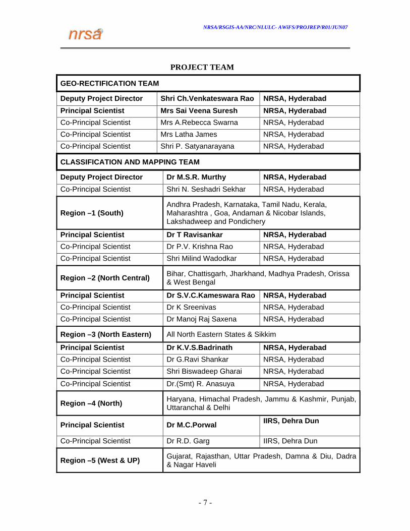
GEO-RECTIFICATION TEAM
Deputy Project Director Shri Ch.Venkateswara Rao NRSA, Hyderabad Principal Scientist Mrs Sai Veena Suresh NRSA, Hyderabad Co-Principal Scientist Mrs A.Rebecca Swarna NRSA, Hyderabad Co-Principal Scientist Mrs Latha James NRSA, Hyderabad Co-Principal Scientist Shri P. Satyanarayana NRSA, Hyderabad
CLASSIFICATION AND MAPPING TEAM
Deputy Project Director Dr M.S.R. Murthy NRSA, Hyderabad Co-Principal Scientist Shri N. Seshadri Sekhar NRSA, Hyderabad
Region –1 (South) Andhra Pradesh, Karnataka, Tamil Nadu, Kerala, Maharashtra , Goa, Andaman & Nicobar Islands, Lakshadweep and Pondichery
Principal Scientist Dr T Ravisankar NRSA, Hyderabad Co-Principal Scientist Dr P.V. Krishna Rao NRSA, Hyderabad Co-Principal Scientist Shri Milind Wadodkar NRSA, Hyderabad
Region –2 (North Central) Bihar, Chattisgarh, Jharkhand, Madhya Pradesh, Orissa & West Bengal
Principal Scientist Dr S.V.C.Kameswara Rao NRSA, Hyderabad Co-Principal Scientist Dr K Sreenivas NRSA, Hyderabad Co-Principal Scientist Dr Manoj Raj Saxena NRSA, Hyderabad
Region –3 (North Eastern) All North Eastern States & Sikkim
Principal Scientist Dr K.V.S.Badrinath NRSA, Hyderabad Co-Principal Scientist Dr G.Ravi Shankar NRSA, Hyderabad Co-Principal Scientist Shri Biswadeep Gharai NRSA, Hyderabad
Co-Principal Scientist Dr.(Smt) R. Anasuya NRSA, Hyderabad
Region –4 (North) Haryana, Himachal Pradesh, Jammu & Kashmir, Punjab, Uttaranchal & Delhi
Principal Scientist Dr M.C.Porwal IIRS, Dehra Dun
Co-Principal Scientist Dr R.D. Garg IIRS, Dehra Dun
Region –5 (West & UP) Gujarat, Rajasthan, Uttar Pradesh, Damna & Diu, Dadra & Nagar Haveli
PROJECT TEAM

NRSA/RSGIS-AA/NRC/NLULC- AWiFS/PROJREP/R01/JUN07
- 8 -
Principal Scientist Dr D.Dutta RRSSSC-Jodhpur Co-Principal Scientist Shri S. Pathak RRSSSC-Jodhpur Co-Principal Scientist Dr Rakesh Paliwal RRSSSC-Jodhpur
GEO-DATABASE CREATION TEAM
Deputy Project Director Dr Y.V.S.Murthy NRSA, Hyderabad Principal Scientist Dr M.V. Ravi Kumar NRSA, Hyderabad Co-Principal Scientist Shri A. Lesslie NRSA, Hyderabad Co-Principal Scientist Shri R.V.N. Srinivas NRSA, Hyderabad Co-Principal Scientist Shri P. Sampath Kumar NRSA, Hyderabad Co-Principal Scientist Shri V.V. Sarath Kumar NRSA, Hyderabad
QUALITY EVALUATION TEAM Deputy Project Director Dr J.R.Sharma RRSSSC-Jodhpur Principal Scientist Shri Vinod Bothale RRSSSC-Jodhpur Co-Principal Scientist Dr S.Jonna NRSA, Hyderabad
Co-Principal Scientist Smt. Rajashree Bothale RRSSSC-Jodhpur
Co-Principal Scientist Shri M.A.Fyzee NRSA, Hyderabad
Co-Principal Scientist Dr Rajeev Jaiswal, EOS, ISRO Hqrs., Bangalore
PROJECT DIRECTOR
Dr P.S. Roy, Deputy Director, RS&GIS - AA, NRSA

NRSA/RSGIS-AA/NRC/NLULC- AWiFS/PROJREP/R01/JUN07
- 9 -
CONTENTS Foreword 2 Acknowledgements 3 Executive Summary 4 Project Team 7
CHAPTER 1 INTRODUCTION 10 -19
1.1 Background 10
1.2 LULC Assessment 1.3 Present LULC Information System 1.4 LULC Classification Methods
11 14 16
1.5 Present Project Initiative 18
CHAPTER 2
METHODOLOGY
20 – 32
2.1 Project Approach 20 2.2 Methodology 20 2.3 Data Products 20 2.4 Geo-rectification 23 2.5 Radiometric Normalization of Satellite Data 25 2.6 Classification and Mapping 26 2.7 Analysis of Satellite Data 28 2.8 Data for Accuracy Assessment 29 2.9 Quality Check Of Classification 29 2.10 Mosaicing And Area Statistics 29 2.11 Geo-database 29
CHAPTER 3 RESULTS
33 – 42
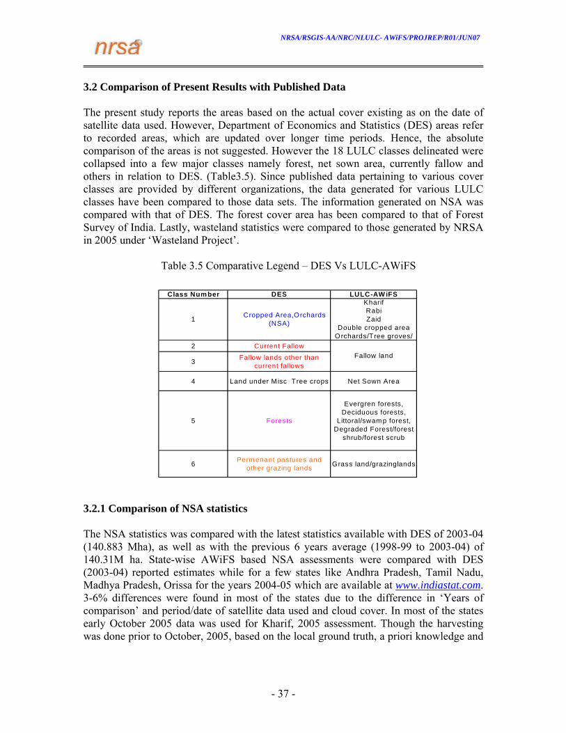
3.1. Classification results 33 3.2. Comparison of Present Results With Reference Data 37 3.3. Accuracy Assessment 39
CHAPTER 4
GEODATABASE ORGANIZATION AND SOFTWARE DEVELOPMENT
43 - 49
4.1 Database Organization 43

NRSA/RSGIS-AA/NRC/NLULC- AWiFS/PROJREP/R01/JUN07
- 10 -
CHAPTER –1 INTRODUCTION
1.1 Background India is bestowed with valuable natural resources consisting of forests, mineral deposits, wetlands, rivers, surface water bodies and vast areas of agriculture serving the needs of around a billion population and varied ecological functions. Due to increase in population, industrialization and with large variations in climate and natural disasters, the natural resources management has become very complex. Since independence the population has increased by 284 per cent (363 to 1033 M) and food grain production by 386 percent (51 to 196 MT). On the other hand, 260 M population still lives below the poverty line .The country has 150 M ha of agricultural area and about 24% GDP is met from the agricultural production. The highly water dependent crop production systems are sensitive to monsoon climate, droughts and cyclones etc. and as well suffers from unscientific irrigation/ fertilization practices as well as pest attacks. Apart from this, trend of switching to commercial non-food grain crops is a cause of concern. While food grain production increased only by 1.7 times over the last two decades, non-food grain production quadrupled during the same period.
The forests, which are mostly of tropical and sub tropical in nature, constitute 64 million hectare and are most sensitive to biotic and climatic factors. The forest vegetation is present in four major ecological zones (Himalayas, Vindhyans, Eastern and Western Ghats) covering different altitudinal and latitudinal regions and their composition is regulated by the monsoon regimes and spatial variability in climate. The forest vegetation is largely disturbed because of the increasing rate of deforestation due to unsustainable extraction of timber, fuelwood and fodder as well as forestland conversions. It is estimated that the timber requirements, which was 68,857 MT in 1980, would rise to 181,270 MT by 2025. Fuel wood stands as the main stay of energy resource for 70% of Indian population and 125 MT are extracted annually. In addition over half of the live stock population (270 M) depend on forest for grazing resources and NTFP worth of Rs. 6.5 – 20 billion is met annually from forest.
The surface water resources support wide ranging natural and manmade biological systems. Hence, play a key role in better management of natural resources. The increased urbanization and abnormal trends of precipitation are severely infringing the overall existence of surface water resources and wetlands across the country. Such seasonal and perennial water bodies serving as backbone of crop production need to be monitored to attain sustainable management of water resources. Apart from these utilitarian resources, wastelands assume significant proportion of land use pattern amounting to 67 M ha out of which cultivable wastes constitutes around twenty per cent. The productive use of these lands would add to the economic and ecological amelioration of the system. Advent of huge planting efforts to harness

NRSA/RSGIS-AA/NRC/NLULC- AWiFS/PROJREP/R01/JUN07
- 11 -
potential of wastelands across country would require effective and regular monitoring of re-greening efforts, to develop better planting schemes and understand limitations. Studies so far conducted in our country are limited in scope, as they cater for base line data towards regional planning and evaluation. The national spatial databases enabling the monitoring of temporal dynamics of agricultural ecosystems, forest conversions, and surface water bodies etc. are lacking. These kinds of databases are primarily important for national accounting of natural resources and planning at regular intervals. Land use and land cover mapping addressing Kharif, Rabi and Zaid crops, greening of wastelands, seasonality of wetlands/surface waterbodies, forest vegetation and other high temporal land use practices using satellite remote sensing data can provide a reliable database. In this context the census of natural resources - land, water, soils, forests and other elements – conducted in a systematic manner and with a repeat cycle to depict changes and modifications as a “snap-shot” of the country’s status of natural resources is realized as an urgent need. 1.2. LULC assessment 1.2.1 Global experiences Varied experiences with regard to LULC mapping have been reported from different continents employing moderate to coarse resolution datasets often in tandem with ancillary databases. The National Mapping Program, a component of the U. S. Geological Survey (USGS), produced LULC maps based on aerial photography of 1970- 1980 on 1:250,000 using hierarchical classification Experiences in China, depict compilation of a 1:1 million scale atlas of Land Use Map of China as the first land-use map for 1991 covering the entire territory based on field surveys, satellite images and aerial photos (Wu, 1991). The National Land Cover Database (NLC) of South Africa was derived (using manual photo-interpretation techniques) from a 1:250,000 scale geo-rectified, single date LANDSAT Thematic Mapper (TM) satellite imagery 1994-95. The Global Vegetation Monitoring unit of the JRC, ISPRA, Italy has produced a new global land cover classification for the year 2000, in collaboration with over 30 research teams from around the world using SPOT 4 vegetation data. Recent exercise of National Land Cover Database for United States known as “Multiresolution Land Characterization 2001 (MRLC 2001) ” has attempted to create an updated pool of Landsat 5 and 7 satellites to generate land cover database (National Land Cover Database, 2001). Another recent attempt on global LULC vegetation is use of MODIS data as one of the critical global data sets. The classification includes 17 categories of land cover following the International Geosphere-Biosphere Program (IGBP) scheme. The set of cover types includes eleven categories of natural vegetation covers broken down by life form; three classes of developed and mosaic lands, and three classes of non-vegetated lands.

NRSA/RSGIS-AA/NRC/NLULC- AWiFS/PROJREP/R01/JUN07
- 12 -
1.2.2 Indian experiences In India the information on LULC in the form of thematic maps, records and statistical figures are inadequate and do not provide an up to date information on the changing land use patterns and processes. Over the years, the efforts made by the various Central / State Government Departments, Institution / Organizations etc., is sporadic and often efforts are duplicated. In most the cases, as the time gap between reporting, collection and availability of data is more, the data often becomes out-dated. However, the organizational efforts in publishing maps, reports and statistical data by various central, state and and other local agencies are noteworthy. 1.2.2.1 Nationwide LULC Analysis for Agro-Climatic Zone Planning NRSA, DOS, taking into consideration the existing land use classification systems(NATMO, CAZRI, Ministry of Agriculture, Revenue Department, AIS & LUS etc),details obtainable from satellite imagery and discussions with nearly 40 user departments / institutions in the country developed a 22 fold classification system for Nationwide LULC mapping. District-wise LULC analysis of all the 15 agro-climatic zones, using the 22 fold LULC classification system was done using 1988 – 89 satellite data sets by NRSA along with Regional Remote Sensing Service Centres (RRSSC’s), State Remote Sensing Centres and other institutions. IRS - LISS-I data of kharif (July-October) 1988 and Rabi (November– March) 1989 were used to generate details of crop land in kharif and rabi seasons, the area under double crop, fallow lands, different types of forest, degradation status, wasteland, water bodies etc. 1.2.2.2National Wastelands Inventory Project (NWIP) National wasteland mapping was carried in five phases. The latest spatially explicit information on 1:50,000 scale was prepared using IRS-LISS III data of 2003-05. About 55.27 million ha (17.45 per cent) have been estimated as wastelands through this study. 1.2.2.3 Forest / Vegetation cover analysis The biennial forest cover mapping is done for the entire country since 1983. FSI has carried out 8 such surveys using satellite imagery of the periods 1981-83 , 1985-87 , 1987-89, 1989-91, 1991-.93, 1993-95 and 1996-97. The latest state forest report (2003) estimated total forest cover as 19.39 per cent of the geographical area of the country. 1.2.2.4 Land Cover Mapping using Spot-Vegetation for South Central Asia Under Global Land Cover (GLC) 2000, Indian Institute of Remote Sensing (IIRS), Dehradun, India has carried out a study for South Central Asian Region as part of this programme. The study has been executed with a participation of network support from countries like China, Sri Lanka, Myanmar, Thailand, Bhutan, Nepal and Bangladesh. The

NRSA/RSGIS-AA/NRC/NLULC- AWiFS/PROJREP/R01/JUN07
- 13 -
study has produced LULC map for South Central Asian Region using SPOT-4 VEGETATION and other ancillary information. 1.2.2.5 Biome level characterization of Indian Vegetation (IRS– WiFS Data) Realising the potential of the IRS – WiFS datasets for regional level mapping, the assessment of phenological growth of vegetation in forest eco system has been attempted under ISRO-GBP programme by Indian Institute of Remote Sensing (IIRS), Dehradun . The climatic data with bio geographic map is used to delineate the biomes in the Indian Sub continent. 1.2.2.6 Vegetation type mapping As part of landscape level biodiversity characterization project (DOS-DBS supported programme) vegetation type mapping of NE regions and Western Ghats on 1 : 250,000 scale was done using IRS-LISS-III satellite data. Central India, Eastern Ghats and East coast are being mapped on 1 : 50,000 scale using IRS P6, LISS-III satellite data 1.2.2.7 Integrated Mission Sustainable Development(IMSD) This is one of the important projects carried out by Department of Space (DOS). It was initiated in 1987 as ‘Integrated Study to Combat Drought’. Under this project different thematic maps viz., LULC, Hydrogeomorphology, Soils, Slope etc. were generated on 1: 50,000 scale and integrated to derive locale specific prescriptions called action plans for sustainable development of land and water resources. The entire work was carried out in three phases covering 175 districts in different agro-climatic zones covering about 84 million ha. or 25% of the total geographical area (NRSA,2002). 1.2.2.8 NRIS project DOS has initiated this project in continuation to IMSD and the digital databases are being prepared for various themes. In this project the standards for database design, structure, theme content and codification were evolved. This project is being implemented in 17 states and all important natural resources including the LULC are being mapped on 1: 50,000 scale using IRS-LISS III data. 1.2.2.9 Integrated Resources Information System for Desert areas(IRIS-DA) This is one of the recent projects carried out at NRSA(2002-2005) for Ministry of Rural Development(MRD). It covers parts of four states – Rajasthan, Karnataka, Gujarat and Haryana. In this project all thematic maps of natural resources are prepared on 1: 50,000 and the action plans for land and water resources development are generated. The LULC theme was mapped upto Level-III classes. In this project the action plans were generated using fuzzy logic and output were generated through an automatic software programmes developed.

NRSA/RSGIS-AA/NRC/NLULC- AWiFS/PROJREP/R01/JUN07
- 14 -
1.2.2.10 Wetlands of India This project is being carried out by SAC, Ahemedabad with the objective of mapping all the wetlands (like marshes, swamps, open water bodies, mangroves, tidal flats etc.) on 1: 250,000 scale for most of the states and on 1: 50,000 scale for few small states and UTs. This project was sponsored by Ministry of Environment and Forests, Government of India. Wetland delineation and mapping has been done using IRS-LISS I/II data of 1992/1993. The total wetland area has been estimated to be 7.6 M ha(excluding Paddy, Rivers and Canals) 1.2.2.11 Land Use / Land Cover inventory under NR Census As part of the national level NR Census Mission, proto type studies were taken up in 13 districts across the country to develop legends in consultation with line departments for mapping various themes, standardization of methodology including digital data base creation and generate census statistics for various natural resources 1.3. Present LULC Information System Information on LULC is traditionally being compiled by Directorate of Economics and Statistics (DES) of Department of Agriculture and Cooperation under the Ministry of Agriculture, following the nine-fold classification system. Amongst various LULC statistics, Agricultural statistics, especially on crop area, production and productivity across different States / regions are required for policy intervention in terms of trade, price support and procurement, domestic and international trade, credit, and insurance. The DES releases crop estimates on annual basis. For the collection of area statistics basically three approaches are followed:
• Complete Enumeration – This method is followed in 17 major states (Andhra Pradesh, Assam (excluding hilly districts), Bihar, Chhattisgarh, Gujarat, Haryana, Himachal Pradesh, Jammu & Kashmir, Jharkhand, Karnataka, Madhya Pradesh, Maharashtra, Punjab, Rajasthan, Tamil Nadu, Uttar Pradesh and Uttaranchal) and 4 UTs (Chandigarh, Delhi, Dadra & Nagar Haveli and Pondicherry) which account for about 86% of the reporting area.
• Sample Survey through a scheme for ‘Establishment of an Agency for Reporting of Agricultural Statistics’ (EARAS) (surveys 20% of villages / investigator zones) account for about 9% of reporting area (Kerala, Orissa, West Bengal, Arunachal Pradesh, Nagaland, Sikkim and Tripura).
• Ad-hoc method - It is based on impressionistic approach of village headman of the reporting area which accounts for 5%. It covers the hilly districts of Assam, the rest of the states in North-Eastern Region (Other than Arunachal Pradesh, Nagaland, Tripura and Sikkim), Goa, Union Territories of Andaman & Nicobar Islands, Daman & Diu and Lakshwadeep).

NRSA/RSGIS-AA/NRC/NLULC- AWiFS/PROJREP/R01/JUN07
- 15 -
Final estimates of crop area and production are available much after the crops are actually harvested (with a time lag of 1-1.5 yrs). Considering the genuine requirement of crop estimates, a time schedule of releasing the advance estimates has been evolved. These estimates of crops are prepared and released at four points of time during a year as mentioned below:
• First Advance Estimates - These estimates are made in the middle of September every year during south-west monsoon season and coincide with the holding of the National Conference of Agriculture for Rabi Campaign. Although there is no specific guideline/methodology issued by the Department of Agriculture & Cooperation (DAC) to make the assessment, these are made by the State Governments based on the reports from the field officer of the State Department of Agriculture. They are mainly guided by visual observations. These are validated on the basis of inputs from the Space Application Center, Ahmedabad, the proceedings of Crop Weather Watch Group (CWWG) meetings, and other feedbacks such as relevant availability of water in major reservoirs, availability/supply of important inputs including credit to farmers.
• Second Advance Estimates – These estimates are made in the month of January every year, the second assessment in respect of Kharif Crops and the first assessment in respect of Rabi Crops.
• Third Advance Estimates - These estimates are prepared towards the end of March/ beginning of April), every year when the National Conference on Agriculture for kharif campaign is convened. The earlier advance estimates of both kharif and rabi seasons are firmed up/ validated with the information available with State Agricultural Statistical Authorities (SASA’s), remote sensing data, reports of Market Intelligence Units (MIU) as well as the proceedings of CWWG.
• Fourth Advance Estimates – These are prepared in the month of June every year when the National Workshop on Improvement of Agricultural Statistics is held and SASAs supply the estimates of both kharif and rabi seasons as well as likely assessment of summer crops. Like third advance estimates, the fourth advance estimates are duly validated with the information available from other sources.
The Directorate of Economics and Statistics (DES) finally brings out every year “Agricultural Statistics At a Glance”. Howerver, the process by which the DES arrives at the agricultural statistics is time- as well as labour-intensive, leading to delayed reporting of the results. Remote sensing data, being amenable to digital classification techniques, facilitate rapid analysis and near-real time assessment of LULC. Various techniques of digital classification of multi-temporal remote sensing images are described below:

NRSA/RSGIS-AA/NRC/NLULC- AWiFS/PROJREP/R01/JUN07
- 16 -
1.4. LULC Classification Methods Using Multi-temporal satellite datasets Multitemporal satellite datasets are used as primary inputs for generation of spatial databases on temporally variant LULC classes. This becomes more relevant when developing regional and national level databases as the LULC classes exhibit varied spatial/temporal characteristics across larger geographical gradients. Hence the extraction of LULC information using multitemporal datasets becomes a complex process due to inherent heterogeneities involved in the datasets and LULC classes. Several parametric and nonparametric digital classification approaches were used to classify multitemporal datasets. 1.4.1 Parametric classification methods Townshend et al. (1987) performed supervised classifications on composited NDVI GAC (Global Area Coverage) data for South America. While they did not validate their results with test data, they found that accuracy for the training sites improved substantially with the increase in the number of images included in the time series. Koomanoff (1989) used annually integrated NDVI values to generate a global vegetation map using NOAA’s Global Vegetation Index product (GVI). This work represents nine vegetation types and does not rely on the seasonality of the NDVI. Reed et al. (1994) and DeFries et al. (1995) have developed and used multi-temporal phenological metrics to derive land cover classifications from AVHRR data. Lambin and Ehrlich (1996a, 1996b) have found that using a time series of the ratio of surface temperature to NDVI provides a more stable classification than NDVI alone, primarily by isolating interannual climatological variability. Loveland et al. (1991, 1995) have produced land cover maps using the International Geosphere-Biosphere Programme (IGBP) classification and Seasonal Land Cover Region (SLCR) classification systems for North America. These maps were based on one year of monthly composited AVHRR-LAC data to generate an unsupervised classification of land cover types for the conterminous United States. The resulting clusters were further stratified based on ancillary environmental data such as elevation and ecoregion. Class labels were assigned based on the temporal curves of the clusters as well as a large number of ancillary sources. Global land cover at 1-degree resolution for 11 land cover classes has been achieved by DeFries and Townshend (1994), Friedl and Brodley (1997), Friedl et al. (1999), and Gopal et al. (1996). These global land cover maps are based on the agreement of the maps of Matthews (1983), Olson (Olson and Watts 1982; Olson et al., 1983) and Wilson and Hendersen-Sellers (1985). 1.4.2 Non-parametric methods To overcome difficulties in conventional digital classification that uses the spectral characteristic of the pixel as the sole parameter in deciding to which class a pixel belongs to, new approaches like context classifiers, decision tree classifiers, neural network algorithms etc. are being developed. In the contextual classification, by considering a

NRSA/RSGIS-AA/NRC/NLULC- AWiFS/PROJREP/R01/JUN07
- 17 -
pixel in the context of its neighboring pixels classification is performed to improve the classification accuracy. Other ancillary data may also be incorporated in order to improve the classification like incorporating a digital elevation model. Another technique is Fuzzy classification in which each pixel is assigned a number for each class, ranging from 0 to1, which indicate the proportions of the different classes which have contributed to the observed spectral signature. A limitation to this program is that the number of end-members that can be employed must be less or equal to the number of input bands. Thus, if the six reflective Landsat TM bands are used, a maximum of six classes can be employed. Neural network and decision tree classifiers are widely used as nonparametric tools. 1.4.3 Neural Networks The use of Neural network classification algorithms are increasing in remote sensing. Unlike the maximum likelihood classifier, they do not rely on the assumption that data are normally distributed. A surface class may be represented by a number of clusters in a feature space plot rather than a single cluster. Remotely-sensed datasets processed by neural network-based classifiers have included images acquired by the Landsat Multispectral Scanner (MSS) (Benediktsson et al., 1990; Lee et al., 1990), Landsat TM (Yoshida and Omatu,1994), synthetic aperture radar (Hara et al., 1994), SPOT HRV (Tzeng et al., 1994) AVHRR (Gopal et al., 1994) and aircraft scanner data (Benediktsson et al., 1993). A number of these studies have also included topography ancillary data (Carpenter et al., 1997), and texture. Many studies have been directed toward recognition of land cover classes, which have ranged from broad life-form categories (Hepner et al., 1990) to floristic classes (Fitzgerald and Lees, 1994).
The bulk of neural network classification work in remote sensing has used multiple layer feed-forward networks that are trained using the back propagation algorithm based on a recursive learning procedure with a gradient descent search. However, this training procedure is sensitive to the choice of initial network parameters and to over fitting (Fischer et al., 1997). The use of Adaptive Resonance Theory (ART) can overcome these problems. Networks organized on the ART principle are stable as learning proceeds, while at the same time they are plastic enough to learn new patterns and improves especially the overall accuracy of classification of multi-temporal data sets (Gopal et al., 1994, Fischer et al., 1997). Recent MODIS based land cover classification uses a class of ART neural networks called fuzzy ARTMAP, for classification, change detection and mixture modeling. 1.4.4 Decision Trees Decision tree classification techniques have been used successfully for a wide range of classification problems. These techniques have substantial advantages for remote sensing classification problems because of their flexibility, intuitive simplicity, and computational efficiency. As a consequence, decision tree classification algorithms are gaining increased acceptance for land cover classification problems, particularly at continental to global scales. Among the advantages of decision trees that are particularly
NRSA/RSGIS-AA/NRC/NLULC- AWiFS/PROJREP/R01/JUN07
- 18 -
useful for remote sensing problems are their ability to handle noisy and missing data (Quinlan, 1993). More commonly, the classification structure defined by a decision tree is estimated from training data using a statistical procedure. A variety of works have demonstrated that decision trees estimated in this type of supervised fashion provide an accurate and efficient methodology for land cover classification problems in remote sensing (Friedl and Brodley, 1997; Hansen et al., 1996; Swain and Hauska, 1977). Lloyd (1990) employed a binary classifier based on summary indices derived from a time series of NDVI data. These phytophenological variables included the date of the maximum photosynthetic activity, the length of the growing season, and the mean daily NDVI value. The variables were fed through a binary decision tree classifier that stratified pixels based first on the date of the maximum NDVI, then the length of the growing season and finally on the mean daily NDVI. DeFries et al. (1998) used decision trees to map land cover using the 8 km AVHRR pathfinder data set with encouraging success. Similarly, Friedl et al. (1999) recently demonstrated that decision trees provide a robust classification methodology for land cover mapping problems at continental to global scales.
As part of GLC 2000 hierarchical classification system was followed involving SPOT 4 vegetation datasets. Global land cover mapping using MODIS data include inputs (i) EOS land/water mask (ii) nadir BRDF-adjusted Reflectance (iii) spatial texture derived from Band 1 (red, 250-meter) (iv) directional reflectance information at 1 km (v) MODIS Enhanced Vegetation Index (EVI) at 1 km (vi) snow cover at 500m (vii) land surface temperature at 1 km and (viii) terrain elevation information. These data are composited over a one-month time period to produce a globally consistent, multi-temporal database on a 1-km grid as input to classification and change characterization algorithms. Processing the 32-days database using decision tree and artificial neural network classification algorithms produces Land cover classes.
Biome level Characterization of Indian vegetation using Multi-temporal IRS WiFS data was done using the decision tree classifier. Distinctive phenological profiles of land covers like coniferous forest, dry deciduous forest, temperate forest, sub-alpine, alpine meadows, orchards, agriculture types were used for classifying land cover categories. The methods included maximum NDVI used in tandem with distinct peaking season to understand ‘green wave’ of land cover elements. The land cover categories were assessed in integration with bioclimatic spatial layers to arrive at biome maps. 1.5 Present Project Initiative Remotely sensed data from space borne platforms especially medium resolution satellites like IRS-P6(AWiFS) and IRS-1D(WiFS) with high temporal resolution (5 days) provide an opportunity to study the dynamics of Land Use and Land Cover. IRS – AWiFS data with multi-spectral bands provide reflectance over green, red, near infrared and middle infrared region. This spectral information over different seasons enables the discrimination of crop and other vegetation more reliably using suitable digital techniques. Spatial data thus generated can be analysed in conjunction with

NRSA/RSGIS-AA/NRC/NLULC- AWiFS/PROJREP/R01/JUN07
- 19 -
administrative and other functional boundaries and also evaluation of intra and inter-annual variations of cropping patterns across the country. In the context of national needs, various advancements in remote sensing data and classification systems, the project is taken up as part of Natural Resources Repository (NRR) activity under National Natural Resources Management System (NNRMS) of Department of Space(DOS), Government of India with the following objective: “Rapid assessment of National Level LULC on 1: 250,000 scale using multi-temporal AWiFS datasets with an emphasis on net sown area for different cropping seasons starting from 2004-05”.
National Level LULC mapping for the crop calendar year 2004 –05 was completed. The project approach, results of 2005-06 and work plan for 2006-07 are presented in this report.
NRSA/RSGIS-AA/NRC/NLULC- AWiFS/PROJREP/R01/JUN07
- 20 -
CHAPTER -2
METHODOLOGY 2.1. Project approach Multi-temporal AWiFS data covering Kharif (Aug –Nov), Rabi (Jan- Mar), Zaid (April- May) seasons were used to address spatial and temporal variability in cropping pattern and other land cover classes. In some of the areas, where the quality of AWiFS datasets was affected by cloud, the datasets were supplemented with WiFS/MODIS datasets.
The multi-temporal datasets were geo-referenced with LCC projection and WGS 84 datum. Later all the satellite datasets were converted into TOA reflectance data to minimize temporal variability.
A hybrid approach involving hierarchical decision tree (See 5), maximum likelihood and interactive techniques were adopted for classification of the data. The legacy datasets on forest cover, type, wastelands and limited ground truth were used as inputs for classification and accuracy assessment.
Geo-database standards were developed to address the issues of retrieval and storage of different data inputs and outputs, designing Meta data elements relevant to different types of data, automated output production and interactive querying. The process based QAS was implemented to regulate the data flows and outputs as per the standards (Fig-2.1).
The Net Sown Area statistics were generated for Kharif cropping season of 2005-06 and integrated LULC map at the end of year. The details of methodology followed for various components of the project are as follows.
2.2 Methodology The methodology followed in the present study is graphically presented in the Fig. 2.2 and briefly described as follows: 2.3 Data Products
Monthly AWiFS data of Aug 05 -May 06 time window was chosen covering the spatial variability of crop and phenological calendars of agriculture and forest ecosystems respectively. Towards this minimum of 150 IRS AWiFS full scenes need to be used. However to augment cloud covered areas and address certain local variabilities, a total 200 IRS AWiFS full scenes comprising of 762 quadrants were used for the second cycle. (Fig –3). The total number used during the cycle is presented in Table 2.1 and Fig 2.3. Based on the experiences in cycle 1 and cloud free data availability, around 100 additional quadrants data were used in 2nd cycle to address early Kharif harvest and extended Rabi. To a limited extent, WiFS and LISS III data sets were also used for cloud infested areas. Precision corrected AWiFS data sets were used as reference database.

NRSA/RSGIS-AA/NRC/NLULC- AWiFS/PROJREP/R01/JUN07
- 21 -
The projection system followed is LCC with the following parameters:
Projection : Lambert Conformal Conic Spheroid : WGS84 Datum : WGS84 1st Parallel : 35 10 22.096000 N 2nd Parallel : 12 28 22.638000 N Longitude of Central Meridian : 80 N Latitude of origin of projection : 24 N False easting : 4000000 metres False Northing : 4000000 metres
Projection :LCC
IRS P6 –AWiFSGeom. regisrtation
NWUM Project Data
F S I Data
Area Statistics
Census 2001 data
Digital Vectors - SOI
Composite LayersComposite Layers
Land use/Land Cover
Admn. Base details Forest Wasteland Demography
DATA MODEL
Projection
Feature Coding
Geodatabase Creation
Quality Assessment
Kharif/Rabi/Zaid
LU/LC Theme Layers
Ground Truth
Digital Classification
Project ApproachProject Approach
1:250 000 Outputs(Sheetwise/Admn boundarywise)
Fig 2.1: Broad Project Approach
Projection :LCC
IRS P6 –AWiFSGeom. regisrtation
NWUM Project Data
F S I Data
Area Statistics
Census 2001 data
Digital Vectors - SOI
Composite LayersComposite Layers
Land use/Land Cover
Admn. Base details Forest Wasteland Demography
DATA MODEL
Projection
Feature Coding
Geodatabase Creation
Quality Assessment
Kharif/Rabi/Zaid
LU/LC Theme Layers
Ground Truth
Digital Classification
Project ApproachProject Approach
1:250 000 Outputs(Sheetwise/Admn boundarywise)
Projection :LCC
IRS P6 –AWiFSGeom. regisrtation
NWUM Project Data
F S I Data
Area Statistics
NWUM Project Data
F S I Data
Area Statistics
Census 2001 data
Digital Vectors - SOI
Census 2001 data
Digital Vectors - SOI
Composite LayersComposite Layers
Land use/Land Cover
Admn. Base details Forest Wasteland Demography
DATA MODEL
Projection
Feature Coding
Geodatabase Creation
Quality Assessment
Feature Coding
Geodatabase Creation
Quality Assessment
Kharif/Rabi/Zaid
LU/LC Theme Layers
Ground Truth
Digital Classification
Project ApproachProject Approach
1:250 000 Outputs(Sheetwise/Admn boundarywise)
Fig 2.1: Broad Project Approach

NRSA/RSGIS-AA/NRC/NLULC- AWiFS/PROJREP/R01/JUN07
- 22 -
Table 2.1. Number of IRS AWiFS data quadrants used for Analysis during 2 cycles
Month No. of AWiFS Products (2004-05)
No. of AWIFS Products( 2005-06)
August 12 62 September 19 51 October 77 89 November 65 79 December 19 93 January 101 80 February 110 81 March 87 86 April 102 64 May 88 77 TOTAL 680 762
Multi-temporalAWiFS data
Georectification
Multispectral Input BandsTemporal Indices
WiFsMODIS
data
Non-availability of
AWiFSProjectionLCC with WGS84
QAS
Integrated LULC data
(Aug-May) data
Rabi(Jan-March) data
Kharif(Aug-Nov) data
GEODATABASE
Accuracy assessment
Decision Tree Classification/MLCLegacy
Data (Forest, wastelands
GroundTruth
AreaStatistics
National & StateLevel maps
QAS
Refinement RefinementIntegrated LULC map
RabiNet Sown
Area
KharifNet Sown
Area
GeodatabaseTOA
reflectancedata
Fig.2. 2. Methodology of Classification
Multi-temporalAWiFS data
Georectification
Multispectral Input BandsTemporal Indices
WiFsMODIS
data
Non-availability of
AWiFSProjectionLCC with WGS84
QAS
Integrated LULC data
(Aug-May) data
Rabi(Jan-March) data
Kharif(Aug-Nov) data
GEODATABASE
Accuracy assessment
Decision Tree Classification/MLCLegacy
Data (Forest, wastelands
GroundTruth
AreaStatistics
National & StateLevel maps
QAS
Refinement RefinementIntegrated LULC map
RabiNet Sown
Area
KharifNet Sown
Area
GeodatabaseTOA
reflectancedata
Fig.2. 2. Methodology of Classification

NRSA/RSGIS-AA/NRC/NLULC- AWiFS/PROJREP/R01/JUN07
- 23 -
Fig 2.3. Number of AWiFS quadrants used during the 1st and 2nd Cycle
0
20
40
60
80
100
120
Augu
st
Sept
embe
r
Oct
ober
Nov
embe
r
Dec
embe
r
Janu
ary
Febr
uary
Mar
ch
April
May
Month
No. of Products(2004-05) No. of Products(2005-06)
2.4 Geo-rectification 2.4.1 Pre-processing Pre-processing of satellite data includes geometric correction, atmospheric correction and radiometric correction. 2.4.1.1 Geometric correction Geometric correction is a process of transformation of a remotely sensed image so that it has the scale and projection properties of a given map projection. is called. A related technique called registration is the fitting of the coordinate system of one image to that of a second image of the same area. Geometric correction of remotely sensed images is required when the image is to be used in one of the following circumstances:
• To transform an image to match a map projection • To locate points of interest on map and image • To bring adjacent images into registration • To overlay temporal sequences of images of the same area, perhaps acquired by
different sensors, and • To overlay images and layers within a GIS.
The main sources of geometric error are: • Instrument error • Panoramic distortion

NRSA/RSGIS-AA/NRC/NLULC- AWiFS/PROJREP/R01/JUN07
- 24 -
• Earth rotation • Platform instability
Instrument errors include distortions in the optical system, non-linearity of the scanning mechanism and non-uniform sampling rates. Panoramic distortion is a function of the angular fields of view of the sensor and affects instruments with a wide angular field of view. Earth rotation varies with latitude. The effect of the earth rotation is to skew the image. Platform instabilities include variations in altitude and attitude. All four sources of error contribute unequally to the geometric distortion present in an image.
The process of geometric correction includes:
• Determination of a relationship between the coordinate system of map and image.
• Establishment of a set of points defining pixel centers in the corrected image that, when considered as a rectangular grid, define an image with the desired cartographic properties, and
• Estimation of pixel values to be associated with those points. The image processing software ERDAS Imagine was used. The AWiFS quadrants were imported. The reference scene path/row scheme identified in which the AWiFS quadrant was covered. If registered adjacent quadrants are available, those scenes were also overlaid on the reference scene and registered with the AWiFS scene. The GCPs were given in such a way that the RMS error is less than 0.5 pixels. For better accuracy and good edge matching between the quadrants, second order polynomial transformation was applied. The re-sampled AWiFS quadrant was overlaid on the reference data and checked by zooming and swiping the scenes. Check was also done by overlaying the adjacent AWiFS scenes too and if the edge-matching was not good, the product was repeated by giving more control points and eliminating the furious points. If good registration was observed, quality Form no. 5 of Annexure VI of the Project Manual was filled and dispatched to the application scientists. While geo-rectifying the quadrant, care is taken such that the quadrant is lying within the Indian boundary. While rectifying the quadrant with reference to the reference data, ground control points (GCPs) are given in the area covered within India only. Hence while checking the accuracy of the quadrant, only points within the Indian terrain were considered. This is clearly entered in the Quality Parameters check form i.e., Form no.5 of Annexure VI of the project manual. For products covered in the plain terrains second order polynomial method was used. In the products of hilly terrains, Area of Interest (AOI) were generated using TIN based model. By this method an accuracy of 3 to 4 pixels is achieved. For Some areas where the cloud free AWiFS data was not available, 1D WiFS data was used, after resampling at 180m pixel size. For Andaman and Nicobar Islands and Lakshadweep islands, LISS3 scenes were generated.

NRSA/RSGIS-AA/NRC/NLULC- AWiFS/PROJREP/R01/JUN07
- 25 -
2.4.1.2 Atmospheric correction Atmospheric effects on electromagnetic radiation add to or reduce the true ground leaving radiance, and act differentially across the spectrum. If estimates of radiance or reflectance values are successfully recovered from remote measurements then it is necessary to estimate the atmospheric effect and correct for it. Such corrections are particularly important - (a) whenever estimates of ground leaving radiances or reflectance rather than relative values are required, for example in studies of change over time, or (b) where the part of the signal that is of interest is smaller in magnitude than the atmospheric component. Considering methodology of post classification comparison of change assessment procedures followed atmospheric correction is not followed in this study. 2.5 Radiometric normalization of satellite data If images taken in the optical and infrared bands at different times (multi-temporal images) are to be studied then one of the sources of variation that must be taken into account is differences in the angle of the sun. A low sun-angle image gives long shadows, and for this reason might be preferred by geological users because these shadows may bring out subtle variations in topography. A high sun angle will generate a different shadow effect. If the reflecting surface is Lambertian, then the magnitude of the radiant flux reaching the sensor will depend on the sun and the viewing angles. For comparative purposes, therefore, a correction of image pixel values for sun elevation angle variations is needed. Such corrections are essential if multi-temporal images are to be compared, for changes in the sensor calibration factors will obscure real changes on the ground. There are a number of physical models for calculating surface reflectance from remotely sensed data; but it is often difficult to get the required inputs at a resolution that is consistent with AWiFS imagery. In this study a hybrid approach was adopted where the “Top-Of-Atmosphere” (TOA) reflectance will be calculated based on a physical model and the AWiFS sensor calibration factors. The calibration steps (Fig 2.4) considered in the radiometric correction procedure for AWiFS imagery are - Gain and offset calibration and sun angle and distance correction. The gain and offset calibration was applied using the gain and offset data provided for each image band. These values for each image band were obtained from AWiFS sensor report. The sun zenith angle for each pixel and the distance from the scene centre to the sun was calculated first, then the reflectance correction was calculated for each band. Conversion from calibrated digital numbers (Qcal) in L1 products back to at-sensor radiance (Lλ) requires knowledge of the original rescaling factors. The following equation is used to perform a Qcal –to-radiance conversion for L1product: ( LMaxλ - LMinλ )
Lλ = ---------------------- Qcal + LMinλ
Qcal max Where, Lλ = Spectral radiance at the sensor’s apperture in W/(m2.sr.µm)

NRSA/RSGIS-AA/NRC/NLULC- AWiFS/PROJREP/R01/JUN07
- 26 -
Qcal = The quantized calibrated pixel value in Digital Number Qcal min = The minimum quantized calibrated pixel value (DN= 0) corresponding to LMinλ Qcal max = The maximum quantized calibrated pixel value (DN=0) corresponding to LMaxλ LMinλ = The Spectral radiance that is scaled to Qcal min in W/(m2.sr.µm) LMaxλ = The Spectral radiance that is scaled to Qcal max in W/(m2.sr.µm)
Fig 2.4 TOA reflectance image generation using AWiFS data sets 2.6 Classification and Mapping The current project envisages use of multi-temporal AWiFS data supplemented with WiFS data, in cloud affected area. In order to bring out the uniformity in the work and in maintaining the high quality outputs, following procedure was adopted: 2.6.1 Input Data Input data consists of satellite data, topographical maps and legacy data. 2.6.2 Satellite data IRS-P6 AWiFS geometrically corrected and converted to TOA Reflectance data formed the basic data. Multi-temporal satellite data of Kharif (August–November), Rabi (January–March) and summer (April–May) were used. Keeping in view the heterogeneity of crop calendar over the entire country even within a season, multi-date satellite data were used.
AWiFS Data in different bands
DN to Radiance Conversion (L) using sensor gain and offset values available in the header file/record
Estimate of TOA Reflectance values ρλ = ∏.Lλ.d2/E0λ.cos(θ)
AWiFS TOA Reflectance image
Solar Zenith angle (θ), Sun-earth distance(d) Solar irradiance values (E0λ)
NRSA/RSGIS-AA/NRC/NLULC- AWiFS/PROJREP/R01/JUN07
- 27 -
2.6.3 Data Preparation The input satellite data were checked for quality as per the data evaluation format and prepared necessary data inputs before proceeding further for classification process. After receiving the geometrically rectified quadrant-wise IRS-P6 AWiFS data they were checked as per the quality standards. If quality was not as per the standards, they were sent back for re-processing. If data were acceptable, TOA reflectance data were generated for each quadrant. On fly mosaic of the ‘state’ was prepared and the data gaps were assessed. The quadrant covering the major part of the state was chosen for a given month and supplemented the remaining area with data from other quadrants of the same sensor. The quadrant data of same sensor and of the same path or adjacent path, if they were close by dates and having radiometry and seasonal uniformity, were mosaiced. The difference between dates of acquisition should be less than 20 days and should not stagger over two crop seasons. Care was taken that vegetation spectral response exists in the scene for a given crop season (Kharif, Rabi or zaid). The datasets were generated based on the above procedure for all the required months of a cropping season depending on cloud free data availability. Prior to the classification it was ensured that 5 km buffer around the state boundary is retained to facilitate border matching of classified outputs. The cloud-free cropped areas, cloud infested areas; harvested agriculture fields over the selected AWiFS data were identified. The cloud infested areas and harvested agriculture fields were supplemented with AWiFS/WiFS/ MODIS/OCM in priority. Cloud and cloud-shadow masks and harvested agriculture areas masks were generated and treated these categories of data sets independently for classification. 2.6.4 Legacy Data and Ground Information Forest cover maps of FSI, vegetation type maps, wasteland and LULC maps prepared as part of different projects carried out by NRSA and other DOS centers were used as inputs for classification. These legacy data sets were prepared meeting the standard accuracy limits with the appropriate ground verification. Hence these data sets were used as major inputs for accuracy evaluation of the project results. In order to ascertain the dynamic LULC categories like agriculture, limited ground truth data was collected for the selected critical areas. 2.6.5 Finalisation of Classes and Development of Legend An exclusive land use/land cover classification was evolved to facilitate an appropriate assessment of all the land use/land cover categories to match the objectives of the project and amenability to digital classification (Table 2.2). The classes in the classification system are hierarchically organized to make them applicable in the required spatial scale and collapsible for comparison with the reported areas; adopted directly by user agencies with refinements at their end. The classification scheme is adopted for extracting information for most possible land use/land cover classes in general and all the

NRSA/RSGIS-AA/NRC/NLULC- AWiFS/PROJREP/R01/JUN07
- 28 -
agricultural seasons in particular and hence enable to repeat the process at regular time intervals. The final legend adopted for use in the project along with the colour scheme is given in following Table 2.2. 2.7 Analysis of satellite data With respect to the generation of second cycle LULC assessment, the focus was essentially laid on highly temporal LULC classes like crop, fallow, water and snow. Considering the one year period as very short to decipher, the changes in forest degradation, land degradation and greening of wastelands was not attempted. However, significant clear cut changes in forests and other class transitions were accounted. From integrated LULC map of first cycle agriculture mask (Kharif, rabi, zaid, double/triple crop and fallow areas) and non-agriculture mask were generated. Training sets of first cycle were modified and fresh signature sets were generated to address the changes in crop and fallow areas. Based on the signatures the classified output was passed through non-agricultural mask of 2004-05 to arrive at crop statistics of 2005-06. However, the localized changes in LULC classes other than crop were also delineated using the second cycle data and first cycle non-agricultural mask is updated. This has resulted in the preparation of an integrated LULC map of 2005-06. The data was classified following a hybrid approach (Decision Tree - See5 or Supervised MXL or both). The selection of a classifier is dependent on the number of temporal datasets available during the season, freedom from cloud/haze, complexity of the terrain and temporal registration errors etc., The classification procedure followed is as per the guidelines given in LULC manualIn North Eastern states, Jammu & Kashmir, Tamil Nadu, and Karnataka the required temporal registration was found to be a limiting factor due to complexity of the terrain. In these states the cropped areas were extracted using the individual months and combined with the other LULC information.
Temporal sat data
Optimal date sat data
State TOA Mosaic of AWiFS data 2005 ( Multispectral datasets)
Training sets of 1 st cycle
Update Training sets
Ground truth of 2 nd cycle
Signature generation
Supervised Classification - MXL
Integrated LULC of 2005 -06
Decision Tree Classification - See 5
Refinement Localized class Conversions Non-Agril mask of 1 st cycle

NRSA/RSGIS-AA/NRC/NLULC- AWiFS/PROJREP/R01/JUN07
- 29 -
Fig 2.5. Flowchart of methodology for assessment of Integrated LULC of 2005-06 2.8 Data for Accuracy Assessment Stratified random points generated through ERDAS Imagine software were used to to assess the accuracy of classification. The number of sample points for each strata for selected based on the proportion of the area. However, a minimum of 20 sample points were considered for each class to estimate the accuracy of the classified output. Ground truth data, legacy maps, and multi-temporal FCC have formed the basis for assessment and generation of Kappa co-efficients.
After classification of the datasets Form 7 of Annexure VI of the project manual were filled and submitted to QAS team. Refinement of crop classification areas obtained from WiFS/MODIS with AWiFS based classification map at the end of the year. . 2.9 Quality Check Of Classification Quadrant-wise / state-wise classified land use / land cover outputs were evaluated by Principal Scientist (PI) and observations were recorded in recorded in QA form 7 Annexure VI of the project manual before sending the same to QAS. QAS team drawn from different centers of DOS has undertaken QAS in different phases and ensured the implementation of QAS observations. 2.10 Mosaicing and Area Statistics All classified quadrant outputs were border matched with respect to uniformity of classes prior to mosaicing. After border matching, the classified data was mosaiced state wise and the area statistics will be generated. 2.11 Geo-database Effective geo-database organization requires storage of the data sets in the repository, described in sufficient detail for subsequent search, query, access and reuse. To meet this goal, the NAS system(network based mass storage system) is utilized in the project for consolidating, storing and managing the final data sets and deliverables of the project. In order to ensure a uniform and streamlined way of data storage, transfer and sharing, file naming conventions are developed and enforced. Relevant metadata elements have been designed using VB and ArcObjects for each type of data set viz. geo-rectified quadrants, TOA quadrants, TOA state mosaics, classified state mosaics, etc ( Fig 6&7 ). To address the need for data security of the stored data sets in the repository, relevant metadata elements for enforcing access control are also incorporated. The project envisages the generation of map outputs in A4, A3 and A0 sizes for map extents defined by country, states, districts and 1o x 1o lat-long grids. The map layouts with necessary cartographic elements for state maps with statistics have been designed and finalized in consultation with the Classification team. A software module has been developed for automatic generation of map outputs using VB and Arc Objects. Tools for

NRSA/RSGIS-AA/NRC/NLULC- AWiFS/PROJREP/R01/JUN07
- 30 -
incorporating data services like search, query, visualization, data download, etc with appropriate access control mechanisms are being developed.

NRSA/RSGIS-AA/NRC/NLULC- AWiFS/PROJREP/R01/JUN07
- 31 -

NRSA/RSGIS-AA/NRC/NLULC- AWiFS/PROJREP/R01/JUN07
- 32 -

NRSA/RSGIS-AA/NRC/NLULC- AWiFS/PROJREP/R01/JUN07
- 33 -
CHAPTER -3
RESULTS 3.1. Classification Results All India LULC classified map and statistics were given in Fig 3.1 and Table-3.1. The detailed LULC statistics (Category-wise in individual states) is presented in Table 3.2. The state-wise classified maps are presented in Annexure A. It can be inferred form the Table 3.1, that during 2005-06 about 43.38 percent of the total geographical area of the country constitutes the Net Sown Area(NSA) (142.56 M ha). Forest cover accounted for 67.42 M ha which is 20.52 percent of the total area. The percent distribution of the major classes is depicted as a pie diagram (Fig.3.2). The state-wise statistics of NSA during 2005-06 were given in Table 3.3. The contribution of three seasonal components of NSA is presented in Figure 3.3. It can be seen from the figure that the Kharif only area constitutes about 40.97 percent of NSA followed by double cropped area (32.94 %). The double cropped area is estimated as 47.67 Mha. Plantations contributed 0.78 percent of the NSA. Among the states, Punjab has the highest percentage of NSA to TGA (about 80 %) while Arunachal Pradesh had the lowest percent (2.75 %). Bihar, Kerala, Haryana, Uttar Pradesh and West Bengal have more than 60 % of Total Geographical Area (TGA) as NSA. Rabi only area was found to be high in Madhya Pradesh, Maharastra Gujarat, and Karnataka. On the other hand, the percentage of Zaid crop areas is more in Bihar, Jharkhand, Punjab and Haryana .The proportion of Double Cropped Area (DCA) to TGA was found to be high in Punjab, Haryana, West Bengal, U.P. and Bihar. The crop area statistics of 2005-06 are compared with that of 2004-05 and presented in Table 3.3 and Fig 3.4. With reference to 2004-05, the NSA has increased from 140.23 Mha to 142.56 Mha with considerable increase states like Andhra Pradesh, Gujarat, Rajasthan, Madhya Pradesh, and Tamil Nadu. The temporal variations in cropping patterns have been accounted through analysis of signatures generated from the IRS AWiFS products covering August-May of the crop calendar. In order to account the early harvest crops especially in Madhya Pradesh, Orissa, Rajasthan, Gujarat state etc, significant data of August and September months have been used. In addition November and December data were also used over the states like Andhra Pradesh, Tamil Nadu, and Karnataka, to address the extended Kharif and early Rabi cropped areas. This has resulted in increased satellite data coverage of second cycle in relation to first cycle. Apart from this, there has been a overall increase in the rainfall condition in the country. Especially in states like Andhra Pradesh, Gujarat, West Rajasthan, Madhya Pradesh etc., there is a significant increase in the rainfall (Table 3.4 and Fig.3.5). The second cycle assessment has been analyzed in conjunction with improved data coverage and changes in rainfall patterns.

NRSA/RSGIS-AA/NRC/NLULC- AWiFS/PROJREP/R01/JUN07
- 34 -
0.00200.00400.00600.00800.00
1000.001200.001400.001600.00
Area in Lakh ha
Kharif
Only
Rabi O
nly
Zaid
Only
Double
/Tripple
Crop
Plantat
ion Total
Fig 3.4 Crop Area Statistics - 2004-05 Vs 2005-06
2005-062004-05
Fig 3.3 Contribution of Seasonal Components of NSA - 2005-06
41.17%
20.84%0.78%
32.83%
4.38% Kharif Only
Rabi Only
Zaid Only
Double/Tripple Crop
Plantation
Fig 3.2 Distribution of Major LULC Classes-2005-06
NSA43.53%
Fallow11.23%
Forest20.88%
Others(incl. Plantations in Assam &
WB)24.37%
NSA
Fallow
Forest
Others

NRSA/RSGIS-AA/NRC/NLULC- AWiFS/PROJREP/R01/JUN07
- 35 -
The increase in net sown area could be due to the rise in both single and double cropped areas under favorable rainfall conditions (spatially, temporally and quantitatively) and increased water flows from the reservoirs in the entire country(Fig 3.4). Also, the availability of cloud-free satellite data at the right time during the crop season was also the reasons for changes in the NSA and helped in improving the estimation of the crop cover. Table 3.4. Rainfall in mm received in different meteorological sub-divisions of India between June and October during 2004 and 2005
Total Rainfall from June to October
Deviation (%) from Normal S.No. Meteorological Sub-divison
2004 Normal 2005 2004 2005
1 Assam & Meghalaya 1508.90 1565.94 1577.60 -3.64 0.74
2 Nagaland, Manipur, Mizoram and Tripura 2014.00 1588.29 940.10 26.80 -40.81
3 Sub-Himalayan W.B and Sikkim 2080.10 2160.14 2093.50 -3.71 -3.09
4 Gangetic West Bengal 1411.60 1275.91 1319.60 10.63 3.425 Orissa 1208.40 1275.59 1351.20 -5.27 5.936 Jharkhand 1231.10 1178.14 594.10 4.50 -49.577 Bihar 817.20 1102.34 779.40 -25.87 -29.308 East Uttar Pradesh 755.00 952.26 767.90 -20.71 -19.369 West Uttar Pradesh 707.40 794.27 673.10 -10.94 -15.26
10 Haryana, Chandigarh and Delhi 429.40 472.37 471.30 -9.10 -0.23
11 Punjab 305.70 513.27 446.60 -40.44 -12.9912 West Rajasthan 161.10 262.57 215.80 -38.64 -17.8113 East Rajasthan 610.20 643.56 573.60 -5.18 -10.8714 West Madhya Pradesh 660.30 895.16 725.80 -26.24 -18.9215 East Madhya Pradesh 940.20 1164.32 1248.10 -19.25 7.2016 Gujarat Region 958.40 882.68 1385.30 8.58 56.9417 Saurashtra and Kutch 412.60 443.32 638.30 -6.93 43.9818 Konkan and Goa 2250.00 3958.46 3340.70 -43.16 -15.6119 Madhya Maharashtra 687.40 652.36 1089.20 5.37 66.9620 Marathwada 587.80 752.75 798.70 -21.91 6.1021 Vidarbha 776.90 995.48 1130.50 -21.96 13.5622 Chattisgarh 1109.10 1255.80 1164.40 -11.68 -7.2823 Coastal Andhra Pradesh 671.60 600.18 1020.80 11.90 70.0824 Telangana 585.60 790.40 1153.10 -25.91 45.8925 Rayalaseema 502.10 517.42 728.50 -2.96 40.8026 Tamil Nadu and Pondicherry 596.10 341.21 555.90 74.70 62.92

NRSA/RSGIS-AA/NRC/NLULC- AWiFS/PROJREP/R01/JUN07
- 36 -
27 Coastal Karnataka 2430.20 4861.87 3101.60 -50.02 -36.2128 North Interior Karnataka 532.60 693.60 721.90 -23.21 4.0829 South Interior Karnataka 649.90 621.46 1095.10 4.58 76.2230 Kerala 1761.20 2167.54 2502.00 -18.75 15.43
Source : web sites of Indian Institute of Tropical Meteorology and Indian Meteorological Department
Total Rainfall (June toOctober)
0.00
500.00
1000.00
1500.00
2000.00
2500.00
3000.00
3500.00
4000.00
Ass
am &
Meg
hala
ya
Nag
alan
d, M
anip
ur, M
izor
am a
nd T
ripur
a
Sub
-Him
alay
an W
.B a
nd S
ikki
m
Gan
getic
Wes
t Ben
gal
Oris
sa
Jhar
khan
d
Bih
ar
Eas
t Utta
r Pra
desh
Wes
t Utta
r Pra
desh
Har
yana
, Cha
ndig
arh
and
Del
hi
Pun
jab
Wes
t Raj
asth
an
Eas
t Raj
asth
an
Wes
t Mad
hya
Pra
desh
Eas
t Mad
hya
Pra
desh
Guj
arat
Reg
ion
Sau
rash
tra a
nd K
utch
Kon
kan
and
Goa
Mad
hya
Mah
aras
htra
Mar
athw
ada
Vid
arbh
a
Cha
ttisg
arh
Coa
stal
And
hra
Pra
desh
Tela
ngan
a
Ray
alas
eem
a
Tam
il N
adu
and
Pon
dich
erry
Coa
stal
Kar
nata
ka
Nor
th In
terio
r Kar
nata
ka
Sou
th In
terio
r Kar
nata
ka
Ker
ala
1 2 3 4 5 6 7 8 9 10 11 12 13 14 15 16 17 18 19 20 21 22 23 24 25 26 27 28 29 30
Met. Sub-Division
Rai
nfal
l in
mm
20042005
Fig 3.5.Meteorological sub-division wise Rainfall distribution
NRSA/RSGIS-AA/NRC/NLULC- AWiFS/PROJREP/R01/JUN07
- 37 -
3.2 Comparison of Present Results with Published Data The present study reports the areas based on the actual cover existing as on the date of satellite data used. However, Department of Economics and Statistics (DES) areas refer to recorded areas, which are updated over longer time periods. Hence, the absolute comparison of the areas is not suggested. However the 18 LULC classes delineated were collapsed into a few major classes namely forest, net sown area, currently fallow and others in relation to DES. (Table3.5). Since published data pertaining to various cover classes are provided by different organizations, the data generated for various LULC classes have been compared to those data sets. The information generated on NSA was compared with that of DES. The forest cover area has been compared to that of Forest Survey of India. Lastly, wasteland statistics were compared to those generated by NRSA in 2005 under ‘Wasteland Project’. Table 3.5 Comparative Legend – DES Vs LULC-AWiFS
3.2.1 Comparison of NSA statistics The NSA statistics was compared with the latest statistics available with DES of 2003-04 (140.883 Mha), as well as with the previous 6 years average (1998-99 to 2003-04) of 140.31M ha. State-wise AWiFS based NSA assessments were compared with DES (2003-04) reported estimates while for a few states like Andhra Pradesh, Tamil Nadu, Madhya Pradesh, Orissa for the years 2004-05 which are available at www.indiastat.com. 3-6% differences were found in most of the states due to the difference in ‘Years of comparison’ and period/date of satellite data used and cloud cover. In most of the states early October 2005 data was used for Kharif, 2005 assessment. Though the harvesting was done prior to October, 2005, based on the local ground truth, a priori knowledge and
Class Number DES LULC-AW iFS
2 Current Fallow
3 Fallow lands other than current fallows
4 Land under Misc Tree crops Net Sown Area
5 Forests
Evergren forests, Deciduous forests,
Littoral/swam p forest, Degraded Forest/forest
shrub/forest scrub
6 Perm enant pastures and other grazing lands Grass land/grazinglands
Fallow land
1
Kharif Rabi Zaid
Double cropped area Orchards/Tree groves/
Cropped Area,Orchards (NSA)

NRSA/RSGIS-AA/NRC/NLULC- AWiFS/PROJREP/R01/JUN07
- 38 -
image properties, the harvested fields were classified into ‘cropped’ areas in certain portions of NE region, Maharashtra and Orissa. The higher values of NSA reported for 2005-06 could be due to the enhanced cropping under high rainfall conditions. The present estimates were also compared with Ministry of Agriculture, Government of India report available at www.indiastat.com. It is observed from the report that the area under food grain production has increased from 120.07 Mha to 121.57 Mha for the period 2004-05 to 2005-06 indicating the general trend in the increase of NSA. 3.2.2 Comparison of Forest statistics Amongst other prominent land use/cover classes, the area under forest cover has been found to be 67.42 Mha, constituting 20.52 percent of total geographic area of the country. National level SFR (2003) of Forest Survey of India (FSI) reported as 67.8 Mha. The SFR 2003 was based on IRS-LISS III satellite data of 2000-01. The difference in estimates could be due to non-inclusion of plantations/orchards/tree groves in the forest cover (included in NSA), period of satellite data used and mapping differences between undulating lands with scrub and scrub/shrub/degraded forests. Most of these areas are in forest fringes and classification is improved significantly in 2nd cycle. Intensive field verification is in process for the areas under mismatch with FSI report and expected to be stabilized in 3rd cycle. 3.2.3 Comparison of wasteland statistics WASTELAND MAPPING PROJECT Under National Wastelands Mapping Mission (NRSA, 2005), NRSA has mapped wastelands, modifying the 13 fold classification system to a new 28 fold classification system where more classes are included to cover the severity of degradation that helps in the wastelands reclamation programmes. The methodology followed was heads-on interpretation of satellite data on 1: 50,000 scale from LISS-III sensor with a spatial resolution of 23.5 m. The project was completed by mid 2005 and the total wastelands estimated in the country are 55.27 M ha.(17.45% of TGA). LULC AWIFS PROJECT An exclusive land use/land cover classification was evolved to facilitate an appropriate assessment of all the land use/land cover categories to match the objectives of the project and amenability to digital classification. There are eighteen classes in the classification systems which are hierarchically organized to make them applicable in the required spatial scale and collapsible for comparison with the reported areas.
COMPARATIVE EVALUATION The spatial distribution patterns, individual class-wise differences, and national/state level statistics were compared. The differences were discussed in relation to classification legend, input data, classification scheme etc.

NRSA/RSGIS-AA/NRC/NLULC- AWiFS/PROJREP/R01/JUN07
- 39 -
The LULC AWiFS wasteland classification scheme was designed to facilitate delineation using digital classification. Major land use based wasteland classes like degraded forests within notified forest boundaries, abandoned jhum with scrub were merged under corresponding land cover class. Similarly, different natural / man-made degradation stages like degraded pastures / grazing land, land affected by salinity, steep sloping areas, barren rocky areas which are not amenable for delineation using digital approach were grouped into ‘Other Wastelands’ in LULC Classification scheme. Basically this category refers all the areas with very marginal / no vegetation cover. Cropped areas in notified forest lands, waterlogged areas and degraded plantation which were considered as wastelands were classified under respective land cover classes in AWIFS Classification Scheme. Sandy areas within the river courses were classified under ‘Other Wasteland’ category in LULC-AWiFS scheme. The wasteland project statistics were regrouped as per the grouping shown in Table 3.6. A comparative evaluation of statistics was presented in Table 3.7. The large difference in Jammu and Kashmir is due to total geographical area considered for the study. In the wasteland project, PoK is not considered, and hence the total wasteland reported are low. In states like Andhra Pradesh, Gujarat, Rajasthan and Uttar Pradesh have also shown significant difference. Marginal grasslands / grazing lands due to AWiFS resolution and digital approaches which could not be delineated were classified as land without scrub in Rajasthan. With reference to total national statistics the difference could be largely attributed to the additional TGA considered in J&K state under LULC-AWiFS project. However, significant differences were found spatially and at individual class wise / state level statistics specifically with reference to land with scrub and land without scrub in states like Andhra Pradesh, Uttar Pradesh and Assam. The LULC-AWiFS project has stabilized the delineation of land with scrub / land without scrub based on Oct – May month data analyzed over two cycles. Hence, the delineation using multitemporal AWiFS data could be considered as were supportive. In addition, it should be also noted that the 5-10 % differences in statistics could be due to different years of data used and the dynamic land features like gullies, land with scrub and without scrub. 3.3. Accuracy assessment The classification outputs were subjected to post classification accuracy assessment. The error matrices of accuracy assessment for different states are presented in Annexure B. The overall classification accuracy is found to be 90.07 % with a range of 86 to 95 % in different states as given in Table 3.8. The assessment is based stratified random sampling approach. Based on the aerial extent of each LULC class and variability of distribution across the state, a suitable sample size is chosen. All the points designated for accuracy assessment were evaluated based on legacy data, established features over FCC and ground truth. Accordingly accuracy assessment matrix was generated for each state. The accuracy assessment tables for different states are enclosed.

NRSA/RSGIS-AA/NRC/NLULC- AWiFS/PROJREP/R01/JUN07
- 40 -
While cropped area classes have shown higher accuracies, the LULC classes like scrub, fallow and other wastelands were found with comparatively lesser accuracies. Delineation of no vegetated categories like current and long fallows purely based on spectral signatures is relatively difficult as they typically belong to different land use categories but for the same land cover category. Further certain areas of Long fallow (land with out scrub), Fallow, Scrubland and Crop categories undergo interclass transitions due to the impact of local land use practices and inter annual climatic variations. Due to this reason, classification of these classes based on short term temporal signatures found relatively difficult affecting the overall accuracy of the classification. Hence LULC system need to be monitored over 4-5 years to develop long term temporal signature profiles to facilitate the categorical delineation of these kinds of high temporal transition classes. This would only result into reliable reference LULC classified product for any subsequent change assessment. The accuracy assessment was done for the 1st and 2nd cycles using the legacy data and limited ground information. The approach was based on the stratified random sampling and the accuracy was reported at the state level. Due to the completion of second cycle classification and to provide change assessment a suitable sampling design is proposed to properly address the change areas. The basic principles adopted for sampling are as follows:
LULC Change Assessment is done based on ‘Post Classification Comparison’ Method.
A Standard Reference Classified Product is used for comparison.

NRSA/RSGIS-AA/NRC/NLULC- AWiFS/PROJREP/R01/JUN07
- 41 -
Wetland
Fallow
Crop
Evergreen Forest
Scrub, Deciduous
Mangroves
Grass lands Past
ures
Command Areas
Plantations
Altitude/Latitude
Temp/RH
Ecological Continuum
Fig. 3.6. Land Cover Heterogeneity, Patchiness, Properties helps In passing through continuum and hence gradients of
Variability vis-à-vis accuracy
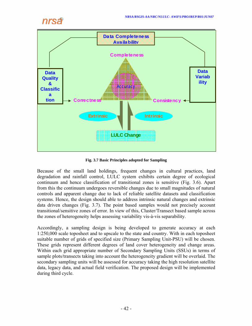
NRSA/RSGIS-AA/NRC/NLULC- AWiFS/PROJREP/R01/JUN07
- 42 -
Fig. 3.7 Basic Principles adopted for Sampling Because of the small land holdings, frequent changes in cultural practices, land degradation and rainfall control, LULC system exhibits certain degree of ecological continuum and hence classification of transitional zones is sensitive (Fig. 3.6). Apart from this the continuum undergoes reversible changes due to small magnitudes of natural controls and apparent change due to lack of reliable satellite datasets and classification systems. Hence, the design should able to address intrinsic natural changes and extrinsic data driven changes (Fig. 3.7). The point based samples would not precisely account transitional/sensitive zones of error. In view of this, Cluster/Transect based sample across the zones of heterogeneity helps assessing variability vis-à-vis separability.
Accordingly, a sampling design is being developed to generate accuracy at each 1:250,000 scale toposheet and to upscale to the state and country. With in each toposheet suitable number of grids of specified size (Primary Sampling Unit-PSU) will be chosen. These grids represent different degrees of land cover heterogeneity and change areas. Within each grid appropriate number of Secondary Sampling Units (SSUs) in terms of sample plots/transects taking into account the heterogeneity gradient will be overlaid. The secondary sampling units will be assessed for accuracy taking the high resolution satellite data, legacy data, and actual field verification. The proposed design will be implemented during third cycle.
Data Completeness Availability
Completeness
Correctness Consistency
LULC Change
Accuracy
Extrinsic Intrinsic
Data Quality
& Classific
a tion
Data Variab
ility

NRSA/RSGIS-AA/NRC/NLULC- AWiFS/PROJREP/R01/JUN07
- 43 -
CHAPTER - 4
GEODATABASE ORGANIZATION AND SOFTWARE DEVELOPMENT
4.1 Database Organization
The basic design and architecture of geodatbase organization plan has been documented and provided in LULC AWiFS project manual. Based on the guidelines, LULC AWiFS Metadata creator software package for Georectified, TOA quadrants, TOA state mosaic and classified outputs using VB & Arc objects are completed. Installation wizard also developed. The software creates metadata XML file and QC related Excel document. It is being tested with 2nd cycle data sets and any further enhancements required will be done. In order to improve the data processing time, software package for TOA parameters extraction was developed for further processing in Erdas Imagine environment for AWiFS data. Subsequently updated the package to version2.0 with enhanced functionality to work with LISS-III and WiFS sensors The existing automatic generation of customized map outputs software package was updated with functionality for districts (A0, A3, &A4 sizes) and 10 x 10 (A0 Size) maps in addition to earlier existing functionality for state mosaics and national mosaics. Automatic validation of input datasets (at the time of batch processing for classified state mosaics) for attribute table errors, data extent, non-availability of datasets and generation of log file (Excel format) for erroneous datasets for further corrections is completed. Created a complete help document on the usage of LULC print module and incorporated in the developed package. Setup & Installation program also developed for the package. The NAS system is being used for both storage of 1st cycle as well as 2nd cycle data sets by all classification teams. The details are as shown below
1st Cycle: LULC –Project for Calendar year 04-05: 277 GB (in NAS)
Geo Rectified Data (Avaliable in CD’s) : 491 CD’s GeoRectified Data in(path/row wise ) : 113 GB TOA Mosiac –State Wise& Classified Data State Wise : 164 GB 2nd Cycle: LULC Project for Calendar Year 05 -06: 522 GB (in
NAS)
NRSA/RSGIS-AA/NRC/NLULC- AWiFS/PROJREP/R01/JUN07
- 44 -
Geo Rectified Data in month wise + TOA data : 503 GB TOA Mosiac - State Wise& Classified Data State Wise : 19.3 GB Web GIS base Information System for LULC Mapping: To enhance the outreach of the project outputs, it is decided to organize the entire spatial data along with attribute data in centralized server system. It was also decided to develop a network base information system to share this data to various user communities. The web GIS technology along with geodatabase concepts has been used for development of LULC-Web: A web enabled Information System for LULC mapping project of NRSA. The developed Information System provides a GIS environment in a simple web browser where the user can access original spatial data (raster as well as vector) without having any specific GIS software in his/her computer. The Information System also provides additional GIS tools for basic GIS analysis like distance measurements, buffer analysis, map composition etc. In addition the other information like census information, LULC statistics, per capita analysis etc.; up to district level is also available in the developed system. The information system provides an interactive graphical user interface in standard web browser for querying and analysis of project outputs along with additional information. The spatial data layers available in LULC-Web are:
LULC Map at 250K (National and state level); Satellite Imagery: AWiFS sensor (State level); State Boundary; District Boundary; Taluk Boundary; Point location of District Head Quarters; Point location of major towns.
The non-spatial data available with LULC-Web are:
LULC statistics up to state and district level; Census information (2001) up to state and district level.
The access to the information in LULC-Web is through various customized query builder. Some of the important queries available in LULC-Web are:
Interactive browsing of LULC map up to original scale (1:250K) using scale rendering;
Basic GIS functionalities like zoom in, zoom out, panning, identify, zoom to full extant etc;
Dynamic query builder for state, district and taluk boundaries; Query on LULC statistics at state and district level; Query on census information at state and district level; Linking of census information with LULC statistics;

NRSA/RSGIS-AA/NRC/NLULC- AWiFS/PROJREP/R01/JUN07
- 45 -
Dynamic graph creation for query outputs; Per capita analysis; Various layer overlays on LULC map; Overlay of satellite imagery on LULC Map; Geo-spatial analysis like distance measurements, buffer analysis etc. are
available; Dynamic legend display for area of interest; Map composition and generation of printable format; Save information at client end etc.
System Architecture of LULC-Web: The system architecture for web base Information system for LULC-Web is given in Fig. 4.1: Fig. 4.1 System architecture for web base Information system for LULC-Web In system architecture of LULC-Web there are two major components i.e. Server side process and client side process. In the server side process we need to configure web server, map server and data server at server system. In the developed system Internet Information Services (IIS 6) of Microsoft Corporation as a web server and Arc Internet Map Server (ArcIMS 9.1) as Map server is used for web interfacing. In the database server level the oracle 9i data server is used for database storage and management with

NRSA/RSGIS-AA/NRC/NLULC- AWiFS/PROJREP/R01/JUN07
- 46 -
Arc Spatial database engine 9.0. The information flow of LULC-Web can be describes as- The client sends a request for spatial data of area of Interest to the web server, the web server redirect this request to map server, the map server search for map services in the service registry, the selected map service redirect the request to data server, the data server select the appropriate data and response to map server through map service the map server converts the spatial data in to web browser compatible format and link the output with web server using servelet connector and the web server send this information to the client. In the client side configuration the client must have network connection with Internet browser application installed in his/her local machine. Query Interface for LULC-Web: The query interface of LULC-Web has been developed for network platform. The Active Server pages (ASP) technology has been used for customization and web application development. The Arc Internet Map server is used for rendering of spatial data into web environment. The HTML viewer of ArcIMS is used for map interface and GIS environment. Various customized GIS tools are available along with help document. Some of important screen shot of the Information System are given below (Fig 4.2):
Fig. 4.2 Home Page of LULC-Web
The home page of the LULC-web is shown above. The basic information about the project is available here along with various links related to LULC mapping project. Blue

NRSA/RSGIS-AA/NRC/NLULC- AWiFS/PROJREP/R01/JUN07
- 47 -
color buttons represents the important highlights of the study. At present LULC map for year 2004-05 is available and for year 2005-06 and 2006-07 is planned to make available in the information system. The static map as .JPEG format is openly available for public domain while access to original data sets is accessible through a user name and password. A secure data login page is available in the information system along with utility for registration for user name password. The highlights of the study in text format, related publications, project approach, project team, web development team and contact information is also available in the home page of the Information system. The Web GIS base query interface is available using authentic user name and password. Once the users will provides his/her authorization information the system will open a LULC map viewer (Fig. 4.3). The queries like state level LULC map, District level statistics and overlay of other information is possible as shown in Fig. 4.4 to Fig. 4.5.
Fig. 4.3. LULC Map viewer
Layer overlay
Map overview window
Query tools and GIS toolbar

NRSA/RSGIS-AA/NRC/NLULC- AWiFS/PROJREP/R01/JUN07
- 48 -
Fig. 4.4. Query and analysis of LULC statistics at state level
Fig. 4.5. Query and analysis of LULC statistics at district level

NRSA/RSGIS-AA/NRC/NLULC- AWiFS/PROJREP/R01/JUN07
- 49 -
Fig. 4.6. Zoom to original scale (1:250K): additional layer overlays (town locations etc)