natural language processing - university of...
TRANSCRIPT

Natural Language Processing
Info 159/259Lecture 3: Text classification 2 (Aug 31, 2017)
David Bamman, UC Berkeley

Generative vs. Discriminative models
• Generative models specify a joint distribution over the labels and the data. With this you could generate new data
P(x, y) = P(y) P(x | y)
• Discriminative models specify the conditional distribution of the label y given the data x. These models focus on how to discriminate between the classes
P(y | x)

Generating
0.00
0.02
0.04
0.06
a amazing bad best good like love movie not of sword the worst
0.00
0.02
0.04
0.06
a amazing bad best good like love movie not of sword the worst
P(X | Y = �)
P(X | Y = �)

Generationtaking allen pete visual an lust be infinite corn physical here decidedly 1 for . never it against perfect the possible spanish of supporting this all this this pride turn that sure the a purpose in real . environment there's trek right . scattered wonder dvd three criticism his .
us are i do tense kevin fall shoot to on want in ( . minutes not problems unusually his seems enjoy that : vu scenes rest half in outside famous was with lines chance survivors good to . but of modern-day a changed rent that to in attack lot minutes
positive
negative

Generative models• With generative models (e.g., Naive Bayes), we ultimately
also care about P(y | x), but we get there by modeling more.
P(Y = y | x) =P(Y = y)P(x | Y = y)�y�Y P(Y = y)P(x | Y = y)
• Discriminative models focus on modeling P(y | x) — and only P(y | x) — directly.
prior likelihoodposterior

RememberF�
i=1xiβi = x1β1 + x2β2 + . . . + xFβF
6
F�
i=1xi = xi � x2 � . . . � xF
exp(x) = ex � 2.7x
log(x) = y � ey = x
exp(x + y) = exp(x) exp(y)
log(xy) = log(x) + log(y)

Classification
𝓧 = set of all documents 𝒴 = {english, mandarin, greek, …}
A mapping h from input data x (drawn from instance space 𝓧) to a label (or labels) y from some enumerable output space 𝒴
x = a single document y = ancient greek

Training data
• “I hated this movie. Hated hated hated hated hated this movie. Hated it. Hated every simpering stupid vacant audience-insulting moment of it. Hated the sensibility that thought anyone would like it.”
“… is a film which still causes real, not figurative, chills to run along my spine, and it is certainly the
bravest and most ambitious fruit of Coppola's genius”
Roger Ebert, North
Roger Ebert, Apocalypse Now
positive
negative

Logistic regression
Y = {0, 1}output space
P(y = 1 | x, β) =1
1 + exp��
�Fi=1 xiβi
�
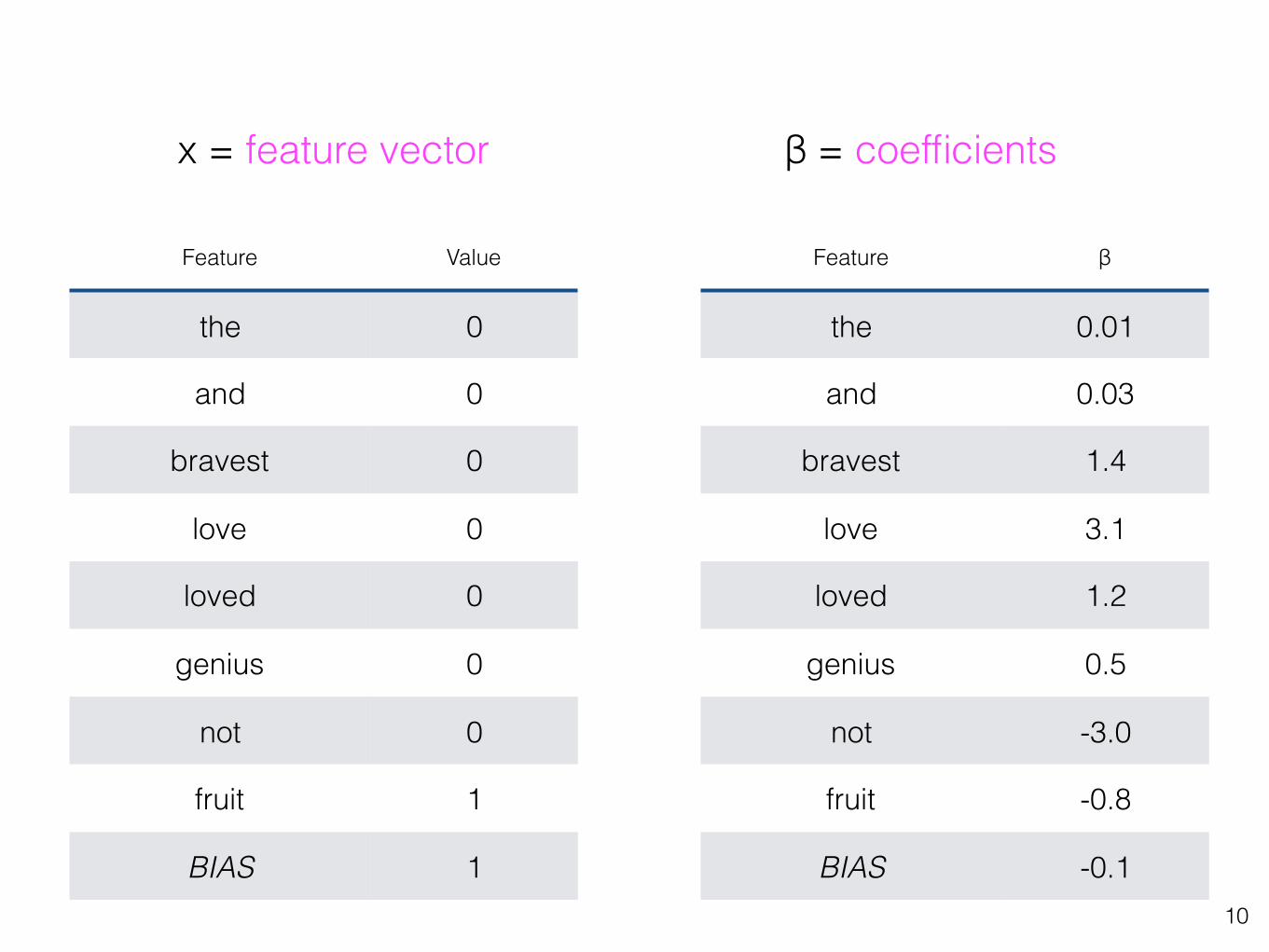
Feature Value
the 0
and 0
bravest 0
love 0
loved 0
genius 0
not 0
fruit 1
BIAS 1
x = feature vector
10
Feature β
the 0.01
and 0.03
bravest 1.4
love 3.1
loved 1.2
genius 0.5
not -3.0
fruit -0.8
BIAS -0.1
β = coefficients

BIAS love loved a=∑xiβi exp(-a) 1/(1+exp(-a))
x1 1 1 0 3 0.05 95.2%x2 1 1 1 4.2 0.015 98.5%
x3 1 0 0 -0.1 1.11 47.4%
11
BIAS love loved
β -0.1 3.1 1.2

• As a discriminative classifier, logistic regression doesn’t assume features are independent like Naive Bayes does.
• Its power partly comes in the ability to create richly expressive features with out the burden of independence.
• We can represent text through features that are not just the identities of individual words, but any feature that is scoped over the entirety of the input.
12
features
contains like
has word that shows up in positive sentiment
dictionary
review begins with “I like”
at least 5 mentions of positive affectual verbs
(like, love, etc.)
Features

13
feature classes
unigrams (“like”)
bigrams (“not like”), higher order ngrams
prefixes (words that start with “un-”)
has word that shows up in positive sentiment dictionary
Features

Feature Value
the 0
and 0
bravest 0
love 0
loved 0
genius 0
not 1
fruit 0
BIAS 114
Feature Value
like 1
not like 1
did not like 1
in_pos_dict_MPQA 1
in_neg_dict_MPQA 0
in_pos_dict_LIWC 1
in_neg_dict_LIWC 0
author=ebert 1
author=siskel 0
Features

15
β = coefficients
How do we get good values for β?
Feature β
the 0.01
and 0.03
bravest 1.4
love 3.1
loved 1.2
genius 0.5
not -3.0
fruit -0.8
BIAS -0.1

Likelihood
16
Remember the likelihood of data is its probability under some parameter values
In maximum likelihood estimation, we pick the values of the parameters under which the data is most likely.

2 6 61 2 3 4 5 6
fair
0.0
0.1
0.2
0.3
0.4
0.5
P( | ) =.17 x .17 x .17 = 0.004913
2 6 6= .1 x .5 x .5 = 0.025
1 2 3 4 5 6
not fair
0.0
0.1
0.2
0.3
0.4
0.5
P( | )
Likelihood

Conditional likelihood
18
N�
iP(yi | xi, β)
For all training data, we want probability of the true label y for
each data point x to high
BIAS love loved a=∑xiβi exp(-a) 1/(1+exp(-a)) true y
x1 1 1 0 3 0.05 95.2% 1x2 1 1 1 4.2 0.015 98.5% 1x3 1 0 0 -0.1 1.11 47.5% 0

Conditional likelihood
19
N�
iP(yi | xi, β)
For all training data, we want probability of the true label y for
each data point x to high
This principle gives us a way to pick the values of the parameters β that maximize the probability of
the training data <x, y>
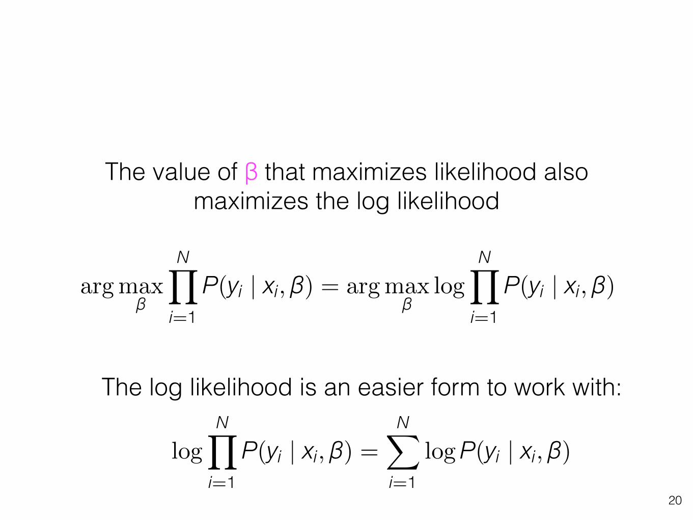
20
The value of β that maximizes likelihood also maximizes the log likelihood
arg maxβ
N�
i=1P(yi | xi, β) = arg max
βlog
N�
i=1P(yi | xi, β)
logN�
i=1P(yi | xi, β) =
N�
i=1logP(yi | xi, β)
The log likelihood is an easier form to work with:

• We want to find the value of β that leads to the highest value of the log likelihood:
21
�(β) =N�
i=1logP(yi | xi, β)

22
�
<x,y=+1>
logP(1 | x, β) +�
<x,y=0>
logP(0 | x, β)
�
�βi�(β) =
�
<x,y>(y � p̂(x)) xi
We want to find the values of β that make the value of this function the greatest

Gradient descent
23
If y is 1 and p(x) = 0.99, then this still pushes the weights just a little bit
If y is 1 and p(x) = 0, then this still pushes the weights a lot

Stochastic g.d.• Batch gradient descent reasons over every training data point
for each update of β. This can be slow to converge.
• Stochastic gradient descent updates β after each data point.
24

Practicalities
�
�βi�(β) =
�
<x,y>(y � p̂(x)) xi
• When calculating the P(y | x) or in calculating the gradient, you don’t need to loop through all features — only those with nonzero values
• (Which makes sparse, binary values useful)
P(y = 1 | x, β) =1
1 + exp��
�Fi=1 xiβi
�
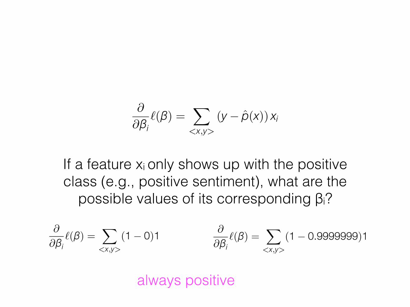
�
�βi�(β) =
�
<x,y>(y � p̂(x)) xi
If a feature xi only shows up with the positive class (e.g., positive sentiment), what are the
possible values of its corresponding βi?
�
�βi�(β) =
�
<x,y>(1 � 0)1 �
�βi�(β) =
�
<x,y>(1 � 0.9999999)1
always positive

27
Feature β
like 2.1
did not like 1.4
in_pos_dict_MPQA 1.7
in_neg_dict_MPQA -2.1
in_pos_dict_LIWC 1.4
in_neg_dict_LIWC -3.1
author=ebert -1.7
author=ebert ⋀ dog ⋀ starts with “in”
30.1
β = coefficients
Many features that show up rarely may likely only appear (by
chance) with one label
More generally, may appear so few times that the noise of
randomness dominates

Feature selection• We could threshold features by minimum count but that
also throws away information
• We can take a probabilistic approach and encode a prior belief that all β should be 0 unless we have strong evidence otherwise
28

L2 regularization
• We can do this by changing the function we’re trying to optimize by adding a penalty for having values of β that are high
• This is equivalent to saying that each β element is drawn from a Normal distribution centered on 0.
• η controls how much of a penalty to pay for coefficients that are far from 0 (optimize on development data)
29
�(β) =N�
i=1logP(yi | xi, β)
� �� �we want this to be high
� ηF�
j=1β2j
� �� �but we want this to be small

30
33.83 Won Bin
29.91 Alexander Beyer
24.78 Bloopers
23.01 Daniel Brühl
22.11 Ha Jeong-woo
20.49 Supernatural
18.91 Kristine DeBell
18.61 Eddie Murphy
18.33 Cher
18.18 Michael Douglas
no L2 regularization
2.17 Eddie Murphy
1.98 Tom Cruise
1.70 Tyler Perry
1.70 Michael Douglas
1.66 Robert Redford
1.66 Julia Roberts
1.64 Dance
1.63 Schwarzenegger
1.63 Lee Tergesen
1.62 Cher
some L2 regularization
0.41 Family Film
0.41 Thriller
0.36 Fantasy
0.32 Action
0.25 Buddy film
0.24 Adventure
0.20 Comp Animation
0.19 Animation
0.18 Science Fiction
0.18 Bruce Willis
high L2 regularization

31
β
σ2
x
μ
y y � Ber
�
�exp
��Fi=1 xiβi
�
1 + exp��F
i=1 xiβi
�
�
�
β � Norm(μ, σ2)

L1 regularization
• L1 regularization encourages coefficients to be exactly 0.
• η again controls how much of a penalty to pay for coefficients that are far from 0 (optimize on development data)
32
�(β) =N�
i=1logP(yi | xi, β)
� �� �we want this to be high
� ηF�
j=1|βj|
� �� �but we want this to be small

P(y | x, β) =exp (x0β0 + x1β1)
1 + exp (x0β0 + x1β1)
P(y | x, β) + P(y | x, β) exp (x0β0 + x1β1) = exp (x0β0 + x1β1)
P(y | x, β)(1 + exp (x0β0 + x1β1)) = exp (x0β0 + x1β1)
What do the coefficients mean?

P(y | x, β)
1 � P(y | x, β)= exp (x0β0 + x1β1)
P(y | x, β) = exp (x0β0 + x1β1)(1 � P(y | x, β))
P(y | x, β) = exp (x0β0 + x1β1) � P(y | x, β) exp (x0β0 + x1β1)
P(y | x, β) + P(y | x, β) exp (x0β0 + x1β1) = exp (x0β0 + x1β1)
This is the odds of y occurring

Odds• Ratio of an event occurring to its not taking place
P(x)1 � P(x)
0.750.25 =
31 = 3 : 1Green Bay Packers
vs. SF 49ers
probability of GB winning
odds for GB winning

P(y | x, β)
1 � P(y | x, β)= exp (x0β0 + x1β1)
P(y | x, β) = exp (x0β0 + x1β1)(1 � P(y | x, β))
P(y | x, β) = exp (x0β0 + x1β1) � P(y | x, β) exp (x0β0 + x1β1)
P(y | x, β) + P(y | x, β) exp (x0β0 + x1β1) = exp (x0β0 + x1β1)
P(y | x, β)
1 � P(y | x, β)= exp (x0β0) exp (x1β1)
This is the odds of y occurring

P(y | x, β)
1 � P(y | x, β)= exp (x0β0) exp (x1β1)
exp(x0β0) exp(x1β1 + β1)
exp(x0β0) exp (x1β1) exp (β1)
P(y | x, β)
1 � P(y | x, β)exp (β1)
exp(x0β0) exp((x1 + 1)β1)Let’s increase the value of x by 1 (e.g., from 0 → 1)
exp(β) represents the factor by which the odds change with a
1-unit increase in x

Room change!• Starting next Tuesday 9/5, we’ll be in 2060 Valley
Life Sciences Building