natural variation in south-eastern south australian small
TRANSCRIPT
Natural variation in south-eastern South Australian small mammal communities through the Late Quaternary
Amy C. Macken BSc (Honours) Botany and Ecology
School of Biological Sciences Faculty of Science and Engineering
Flinders University of South Australia
9 August 2013
Supervisors: Dr Elizabeth Reed (principal) Dr Gavin Prideaux (associate)
Submitted in fulfilment of the requirements for the degree of Doctor of Philosophy

ii
For my grandma, Jean Le Cornu, who inspires me to persist against all odds, and the memory of my late grandpa, Deane Le Cornu,
from whom I draw the strength to do so.

iii
© Copyright by Amy C. Macken 2013 All Rights Reserved
iv
Declaration I certify that this thesis does not incorporate without acknowledgment any material
previously submitted for a degree or diploma in any university; and that to the best
of my knowledge and belief it does not contain any material previously published or
written by another person except where due reference is made in the text.
I give consent to this copy of my thesis when deposited in the University Library,
being made available for loan and photocopying, subject to the provisions of the
Copyright Act 1968.
I acknowledge that copyright of published works contained within this thesis (as
listed below) resides with the copyright holder(s) of those works.
List of publications: Macken, A.C., McDowell, M.C., Bartholomeusz, D.H. & Reed, E.H. (2013)
Chronology and stratigraphy of the Wet Cave vertebrate fossil deposit, Naracoorte,
and relationship to paleoclimatic conditions of the Last Glacial Cycle in south-
eastern Australia. Australian Journal of Earth Sciences 60, 271–281.
Macken, A.C., Staff, R.A. & Reed, E.H. (2013) Bayesian age-depth modelling of
Late Quaternary deposits from Wet and Blanche Caves, Naracoorte, South
Australia: a framework for comparative faunal analyses. Quaternary
Geochronology 17, 26–43
Macken, A.C & Reed, E.H. (2013) Late Quaternary small mammal faunas of the
Naracoorte Caves World Heritage Area. Transactions of the Royal Society of South
Australia 137, 53–67.
Signed ............................................
Amy Macken
Date ................................................
v
Abstract Natural variation is characterised as the normal types of change that occurs within
ecosystems in response to disturbances at different spatial and temporal scales. Such
changes may be expressed across a range of ecological attributes including
community structure and composition. Changes in these attributes are often argued
to provide the basis of ecosystem resilience to disturbance; that is, the ability of
communities to adapt and reorganise whilst retaining their functional and structural
traits. Consequently, the maintenance of natural variation within ecological systems
has emerged as a primary biodiversity conservation strategy. However, our
understanding of what normal patterns of variation may be expected in different
ecosystems and the constraints on resilience within them, remains limited.
Palaeoecological deposits have increasingly been used to fill knowledge gaps about
the range, type and extent of natural variation and resilience expressed by
ecosystems over long time scales in response to disturbances such as climate
change. Using two owl-pellet derived fossil assemblages of the Naracoorte Caves in
south-eastern South Australia, this thesis examined patterns of natural variation and
resilience of a small mammal palaeocommunity in terms of richness, composition,
structure and relative abundances through the last glacial cycle (c. 51.4 to 10.2 kyr
BP). More specifically, this thesis addressed the following questions:
(a) Did the small mammal palaeocommunity reorganise in response to climate
change associated with the last glacial cycle?
(b) How did variation in different ecological variables contribute to the
persistence or reorganisation of the palaeocommunity, and
(c) How did sampling variation within and between sites, and temporal
resolution, impact patterns detected in the fossil assemblages?
To address these questions, the stratigraphic and chronological contexts of the fossil
assemblages were defined using sedimentary principles and age-depth modelling of
radiocarbon data. Both deposits were found to be composed of five un-reworked
sedimentary units which were statistically correlated between the two sites based on
modelled ages. These units provided a coarse temporal scale corresponding to the
major climatic phases of the last glacial cycle. Sedimentary layers were identified
vi
within the stratigraphic units, providing a finer temporal scale for evaluating the
faunal assemblage.
Faunal analyses showed that the two small mammal assemblages were statistically
similar and exhibited very little compositional or structural change through the early
glacial period and last glacial maximum (LGM). However, two episodes of
significant palaeocommunity reorganisation were revealed at the finer temporal
scale through the deglaciation/late glacial period. These changes were associated
with (a) sea-surface temperatures (SSTs) warming past 16°C, post-dating the onset
of warming following the LGM by c. 1 to 3 kyrs and (b) continued warming of
mean SSTs past 18°C.
The relative abundances of individual species were sensitive to sampling effects and
were variable through time at both temporal scales. The whole-palaeocommunity
metrics were more robust and showed that a palaeocommunity can be stable for
thousands of years, despite variable climatic conditions. Palaeocommunity change
during the deglaciation shows that it is not disturbance per se that led to shifts
between community states, but disturbance beyond palaeoclimatic thresholds within
which particular states were able to persist. Further study of environmental
thresholds for the palaeocommunity and individual species will be valuable for
assessing the variability of species-environmental associations through time and the
potential for their adaptation into the future.
vii
Acknowledgements First and foremost I acknowledge the support, guidance and insight of my principal
supervisor, Dr Liz Reed. I thank her for providing access to resources, support with
funding and for the opportunity to study the small mammal fossils that she
methodically excavated from Blanche Cave. Most importantly, I acknowledge Liz’s
contribution to the project through the sharing of ideas and critique of my work. I
am grateful to Liz for her unwavering confidence in the project and in me, which
gave me the space and freedom to grow personally and professionally. I am also
grateful for the support of my associate supervisor, Dr Gavin Prideaux. Gavin
provided advice and feedback throughout my candidature and was always available
at short notice to help with small, day-to-day problems and more complex questions
associated with my research.
The majority of the work completed for this thesis benefited from the contributions
and advice of collaborators and I extend my gratitude to those who worked with me
on different aspects of the project: Dr Richard Staff who worked with me to
produce the age-depth models for Wet and Blanche caves. Without his help, my
ideas would not have made it to reality. Richard was generous with his time and
knowledge and I am incredibly grateful for his commitment to teaching and guiding
me through each step of the modelling, and for making me laugh along the way. Dr
Matthew McDowell of Flinders University was a collaborator, friend and support
through my candidature. I am grateful to Matt for his good-will as I revisited a site
and fossil collection that he had previously studied. This project was only possible
because of the previous work that had been completed on Late Quaternary aged
sites of the Naracoorte Caves in which Matt was instrumental. I also thank him for
allowing me to use unpublished data from his Masters thesis to complete the review
of the Wet Cave stratigraphy. David Bartholomeusz led the excavation of the Wet
Cave assemblage in 1997/1998. His field note books were vital for reconstructing
the Wet Cave stratigraphy and I am grateful for his involvement in the Wet Cave
review. For collaborating and taking the risk with me on a conference review paper,
I thank Dr Patrick Moss, Dr Graeme Armstrong, Phuong Doan, Dr Beth Gott, Rosie
Grundell, Dr Chris Johnson, Dr Matthew McDowell, Dr Jamie Wood and Dr Craig
Woodward.
viii
I am privileged to have been mentored and supported by highly experienced
palaeontologists throughout my candidature. For their ongoing encouragement and
advice I thank Emeritus Professor Rod Wells, Dr Trevor Worthy, Dr Alex Baynes
and Steve Bourne. I am also grateful to have been surrounded by a diverse group of
colleagues who provided encouragement, feedback on drafts and ideas, help with
sorting and many laughs along the way. This wonderful ‘team’ included members
of the Flinders University Palaeontology Lab and the broader Adelaide
palaeontology community: Grant Gully, Dr Matt McDowell, Rachel Correll, Carey
Burke, Dr Aaron Camens, Sam Arman, James Moore, Aidan Couzens, Elen Shute,
Qam Nasrullah, Sean Adams, Dale Nelson, Celine Caris, Dr Graham Medlin, Dr
Erick Bestland, Dr Nic Rawlence and Dr Maria Zammit; present and former staff of
the Naracoorte Caves National Park: Deborah Craven-Carden, Decima McTernan,
Jen McClean, Alison Rowe, Frank Bromley, Gavin Kluske, Barb Lobban, Julie
Stone, Yarrow Lee, Jinhwa Lee, Ros Jones, Matt Crewe and Andrew Hansford and
Friends of the Naracoorte Caves, Ann and Alan Attwood.
I also extend warm thanks to present and former staff of Flinders University who
patiently answered my questions, helped me with access to resources, guided me
through the paperwork, solved my IT problems and made Flinders warm and
welcoming. This includes Maya Roberts, Kimberley Clift, Elke Eckhard, Sandra
Marshall, Annie Flynn, Diane Colombelli-Négrel, Lyn Spencer, Mike Bull, Pam
Stainer, John Marshall, Russell Stainer, Jenny Brand, Sonia Kleindorfer, Brett
Norsworthy, Raphael Russell-Livingstone, Andrew Daddow and the staff of the
Document Delivery services unit of the Flinders University Library. I also thank
Pawel Skuza for his advice on a range of statistical approaches and for pointing me
towards resources that proved invaluable to my research.
I am also grateful to have had the support of palaeoecologist, Dr Jessica Blois over
my candidature. Jessica generously gave me a crash course in using the program R
and provided me with a copy of an R script that she constructed for her own PhD.
These resources were vital for the faunal analyses completed in this thesis. I also
thank her for sharing her own experiences in research, publishing and coordinating
collaborative projects. Our discussions have stuck with me and will be a source of
advice and guidance for years to come.
ix
Collection managers and curators of mammal collections from museums across
Australia were also generous in sharing their data for use in constructing species
distribution maps (Appendix F) and for allowing access to specimens for
comparison. I especially thank David Stemmer of the South Australian Museum and
Sandy Ingleby of the Australian Museum.
I also acknowledge financial support that has come from a wide range of sources.
This includes an Australian Government Post-graduate Award and a top-up
scholarship from the Playford Memorial Trust. The Linnean Society of New South
Wales provided me with funding for radiocarbon dating. I have also been privileged
to attend conferences of the Ecological Society of Australia with financial support
from the Society, Flinders University of South Australia, the Australian Federation
of Graduate Women and the research funds of Dr Liz Reed. I also attended
workshops in palaeoecology/phylogenetics at the expense of the Australian Institute
of Nuclear Science and Engineering and The National Postgraduate Workshop in
Systematics. The research presented in the thesis was also supported through the
Australian Government Caring for Our Country funding scheme (project: OC11-
00487) and a grant from the Nature Foundation SA Inc. awarded to Dr Liz Reed.
Finally, I extend warm thanks to my family and friends. They were and remain a
source of strength, confidence, motivation and inspiration. To Indigo and Joey,
thank you for always being ready with an open ear, warm tea and thoughtful words.
Julie, Sue and Grandma, thank you for being model to me of strong, successful
women. To my dad, Michael, thank you for wanting only the best for me, and to my
mum, Cathy, for your confidence and endless support. It gives me more strength
than you could imagine. Thank you too for sharing in my successes and for
consoling me when things didn’t go as planned. And to my partner, James, thank
you for being my ally, for believing in me and being ready with open arms and ears
every day of the last three and a half years. This thesis is better for my having been
able to share it with you.

x
Contents
Declaration ................................................................................................................ iv Abstract ...................................................................................................................... v Acknowledgements ................................................................................................... vii
1. Introduction .......................................................................................................... 1 Fossil deposits of the Naracoorte Caves World Heritage Area .............................. 2
Faunal responses to Pleistocene climate change ................................................ 4 Application to biodiversity conservation ........................................................... 5
Study Assemblages ................................................................................................. 7
Aims ....................................................................................................................... 9 Supporting objectives ......................................................................................... 9
Thesis Structure .................................................................................................... 13 Introduction to the literature review ................................................................. 13 Introduction to the research chapters, style and progression ............................ 13
2. Literature Review ............................................................................................... 17 Natural variation in (palaeo)ecological assemblages: scale, measurement and interpretation. ......................................................................................................... 17
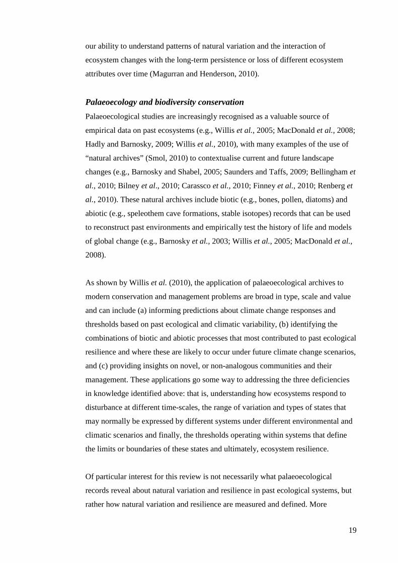
Introduction .......................................................................................................... 17 Climate change: biodiversity adaptation and resilience ................................... 17 Palaeoecology and biodiversity conservation .................................................. 19
Fossil deposits of the Naracoorte Caves World Heritage Area ............................ 21 Scientific and natural history values ................................................................ 21 Geological Context ........................................................................................... 22 Palaeontological Research ................................................................................ 24
Palaeoecology of the NCWHA ............................................................................ 39 Palaeoenvironmental reconstructions ............................................................... 39 Climate change effects on local faunas ............................................................ 44
Defining natural variation and resilience in palaeoecological systems ................ 52 Resilience of Naracoorte mammal faunas to past climate change ................... 52 Natural variation/resilience framework ............................................................ 53 Numeric and ecological hierarchy of natural variation .................................... 55
Forward projection of trends: challenges and potential ....................................... 59
3. Chronology and stratigraphy of the Wet Cave vertebrate fossil deposit, Naracoorte, and relationship to paleoclimatic conditions of the Last Glacial Cycle in south-eastern Australia ........................................................................... 61
Abstract ................................................................................................................ 63
Introduction .......................................................................................................... 64
Site Description, Excavation and Original Sedimentary Analysis ....................... 65 Geological Setting ............................................................................................ 65 Excavation ........................................................................................................ 65 Sedimentary Analysis ....................................................................................... 67
Methods ................................................................................................................ 67
xi
Stratigraphic sequence ...................................................................................... 67 Radiocarbon Dating .......................................................................................... 69
Results .................................................................................................................. 71 Sedimentary Sequence and Chronology........................................................... 71
Discussion ............................................................................................................ 75 Relationship to other Upper Pleistocene sequences of the NCWHA ............... 75 Paleoclimatic Context....................................................................................... 76
Conclusions .......................................................................................................... 84
Acknowledgements .............................................................................................. 85
4. Bayesian age-depth modelling of Late Quaternary deposits from Wet and Blanche Caves, Naracoorte, South Australia: a framework for comparative faunal analyses ........................................................................................................ 86
Abstract ................................................................................................................ 88
Introduction .......................................................................................................... 88
Regional Setting and Study Sites ......................................................................... 91 Geological setting of the Naracoorte Caves ..................................................... 91 Wet Cave (5U10, 11)........................................................................................ 93 Blanche Cave (5U4, 5, 6) ................................................................................. 95
Materials and Methods ......................................................................................... 99 Bayesian age-depth models .............................................................................. 99 Correlation of Wet and Blanche Cave Phases ................................................ 104
Results ................................................................................................................ 104 Wet and Blanche Cave Bayesian Models....................................................... 104 Phase Durations and Potential Hiatuses ......................................................... 105 Correlation of Wet and Blanche Cave Phases ................................................ 117
Discussion .......................................................................................................... 119 Wet and Blanche Cave Bayesian age-depth model priors ............................. 119 Outliers ........................................................................................................... 121 Phase durations, hiatuses and chronological interpretation............................ 125 Correlation of Wet and Blanche Cave Phases ................................................ 128
Conclusion .......................................................................................................... 130
Acknowledgements ............................................................................................ 131
5. Late Quaternary small mammal faunas of the Naracoorte Caves World Heritage Area ........................................................................................................ 132
Abstract .............................................................................................................. 133
Introduction ........................................................................................................ 133
Methods .............................................................................................................. 135 Study site ........................................................................................................ 135 Fossil assemblages ......................................................................................... 137 Accumulation mode ....................................................................................... 139 Species identification ..................................................................................... 140
Results ................................................................................................................ 141 Diversity ......................................................................................................... 141
xii
Discussion .......................................................................................................... 145 Late Quaternary small mammal diversity ...................................................... 145 Faunal turnover and biogeographic implications ........................................... 146 Fossil records as biodiversity baselines for conservation .............................. 148
Conclusion .......................................................................................................... 149
Acknowledgements ............................................................................................ 150
6. Late glacial reorganisation of a small mammal palaeocommunity in southern Australia reveals thresholds of change ............................................... 151
Abstract .............................................................................................................. 152 Introduction ........................................................................................................ 153
Study region ................................................................................................... 158 Geological setting of the Naracoorte Caves ................................................... 161 Chronology and stratigraphy of Wet and Blanche caves ............................... 161
Methods .............................................................................................................. 163 Sample collection and fossil identification .................................................... 163 Faunal analysis: data standardisation ............................................................. 165 Faunal analysis: whole-palaeocommunity and individual species variables . 166 Faunal analysis: site- and time-effects ........................................................... 167 Palaeoclimatic and environmental context ..................................................... 169
Results ................................................................................................................ 170 Data summary................................................................................................. 170 Sampling variation of the local palaeocommunity: site-effects ..................... 170 Macroscale time-effects on palaeocommunity metrics .................................. 177 Mesoscale time effects on palaeocommunity metrics .................................... 178 Time-effects on individual species relative abundances ................................ 182
Discussion .......................................................................................................... 187 Similarity of Wet and Blanche Cave fossil assemblages: palaeocommunity variables.......................................................................................................... 187 Similarity of Wet and Blanche Cave fossil assemblages: relative abundance of individual species ........................................................................................... 188 Macro- versus mesoscale patterns of natural variation, persistence and intrinsic thresholds of change ....................................................................................... 190 Palaeoclimatic and environmental thresholds ................................................ 193
Conclusions ........................................................................................................ 200
Acknowledgments .............................................................................................. 201
7. Concluding Discussion ..................................................................................... 203 Stratigraphic and temporal analyses (chapters three and four) .......................... 204
Late Quaternary small mammal faunas of the Naracoorte Caves (chapters five and six) ............................................................................................................... 208
Final Synthesis ................................................................................................... 217
Appendix A ............................................................................................................ 223 Appendix B ............................................................................................................. 247 Appendix C ............................................................................................................. 251 Appendix D ............................................................................................................ 257

xiii
Appendix E ............................................................................................................. 277 Appendix F ............................................................................................................. 296 References .............................................................................................................. 299
1
1. Introduction Palaeoecology is concerned with the reconstruction and interpretation of past
environments and ecological communities across space and time. ‘Natural archives’
preserved within palaeoecological sites are critical to these reconstructions and
include biotic (e.g., bones, pollen, diatoms, charcoal) and abiotic (e.g., speleothem
cave formations, stable isotopes) records of past life and climatic conditions (Smol,
2010). When natural archives are chronologically and stratigraphically constrained,
they can be used to gain insight into patterns of species diversity, the timing and
role of disturbances in ecosystem development and patterns of extinction and
diversification over timescales spanning decades to millennia (Brenchly and Harper,
1998; Barnosky et al., 2003; Willis et al., 2005; MacDonald et al., 2008).
In exposing links between ecological diversity and drivers of assemblage patterns in
space and time, natural archives may also be used to address questions associated
with biodiversity conservation. The contribution of palaeoecology to biodiversity
conservation has been extensively reviewed, firmly establishing the benefits of
palaeoecology to contemporary biodiversity crises (e.g., Willis et al., 2005; Lyman,
2006; Willis et al., 2007; Rull, 2010; Willis et al., 2010; Vegas-Vilarrbuia et al.,
2011; Appendix A). For example, palaeoecological archives have been used to (a)
set conservation baselines (e.g., Foster et al., 1996; Davis et al., 2007; Burbidge et
al., 2008; Saunders and Taffs, 2009; Bellingham et al., 2010), (b) establish past
rates and direction of ecosystem change to inform predictions and models about
future effects (Barnosky et al., 2003; Carrasco et al., 2009; Davies et al., 2009;
Finney et al., 2010; Willis et al., 2010); (c) determine the extent and rates of
contemporary extinctions against historical baselines (Graham and Grimm, 1990;
Braithwaite and Muller, 1997; McKinney, 1997; Williams, 1997; Bilney et al.,
2010) and (d) isolate climatic from human drivers of change (Barnosky et al.,
2004a; Renberg et al., 2009). Appendix A presents a conference review manuscript
prepared during the course of the research presented in this thesis, highlighting
examples of palaeoecological research applied to biodiversity conservation
problems within Australia and New Zealand.
2
As shown in the examples described in Appendix A, palaeoecological archives
commonly used for specific conservation and management problems are those
derived from lake and peat cores containing pollen, diatoms, phytoliths and other
fine-scale records of past environments. However, vertebrate fossil assemblages,
particularly those preserved in caves and rock shelters, have made significant
contributions to understanding the nature of faunal responses to Quaternary climate
change at the species and community level in Australia (e.g., Prideaux et al., 2007;
Price and Sobbe, 2005; Price and Webb, 2006; Baynes and McDowell, 2010;
McDowell et al., 2013; Price, 2012). In some cases, these records have been used to
address contemporary biodiversity problems, both directly and indirectly, through
the examination of Pleistocene extinctions and long-term community dynamics.
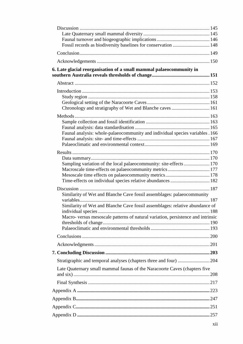
Fossil deposits of the Naracoorte Caves World Heritage Area The palaeoecological archives of interest to this thesis derive from the vertebrate
fossil deposits of the Naracoorte Caves World Heritage Area (NCWHA). The
NCWHA in south-eastern South Australia provides extensive records of faunal
diversity over the Quaternary period (Fig. 1.1). The World Heritage Area contains
26 known caves with over 100 fossil sites among them (Reed and Bourne, 2000).
The oldest vertebrate assemblage from this locality is dated to the Middle
Pleistocene (528±41 ka; Prideaux et al., 2007), while the youngest known in situ
fossil remains have recently been dated to the late Holocene (<1000 yr BP; Macken
and Reed, 2013).
Research into fossil assemblages of the Naracoorte Caves has contributed to
knowledge of (a) late Quaternary faunal communities of southern Australia (e.g.,
Reed and Bourne, 2000; 2009), (b) the taxonomy and systematics of extinct and
living faunas (e.g., Prideaux and Wells, 1998; Williams, 1999; Prideaux, 2004), (c)
vertebrate taphonomy of cave deposits (e.g., Reed, 2006; 2009) and (d)
environmental change over the Quaternary (e.g., Forbes and Bestland, 2007,
Darrénougué et al., 2009).The scientific and natural history values of the cave
deposits are reflected in not only the publications associated with this research but
their World Heritage Listing and extensive on-site interpretation materials.

3
Figure 1.1 Location of the Naracoorte Caves World Heritage Area in south-eastern South Australia,
Australia.

4
Faunal responses to Pleistocene climate change Despite a general bias in palaeoecological studies in Australia towards the causes of
‘megafauna’ extinction, research into the faunas of the Naracoorte Caves has
included smaller body-sized taxa, particularly in faunal based reconstructions of
palaeoenvironmental conditions. For example, the first palaeoenvironmental
reconstructions for the NCWHA were based on the habitat characteristics of small
vertebrates (Smith, 1971; 1972). More recent studies of last glacial aged deposits (c.
50 to 1 kyr BP) used a similar approach, but in a quantified framework based on the
ecological characteristics of the faunas preserved in the assemblages (McDowell,
2001; Laslett, 2006).
A significant focus of research at Naracoorte has also been on the effects of
Pleistocene climate change on local mammal faunas (e.g., Prideaux et al., 2007;
Macken et al., 2012). The first appraisal of faunal responses to Pleistocene climate
change was reported by Moriarty et al. (2000) and represented an important shift in
the type of research question being addressed through analysis of the Naracoorte
Caves fossil faunas; that is, rather than reconstructing climatic and environmental
conditions based on the fossil assemblages, Moriarty et al. (2000) were the first to
consider the effects of changing conditions on the fauna themselves.
In their assessment of the composition of six Middle Pleistocene aged assemblages
of the NCWHA, Moriarty et al. (2000) concluded that there had been “little
apparent change in faunal diversity over a period of 300 ka in the Middle
Pleistocene, a period spanning at least three glacial-interglacial cycles” (p. 141).
The implications of this assessment have been significant in the broader view of not
only the Naracoorte Cave deposits, but discussions of faunal dynamics through the
Pleistocene. For example, the apparent lack of faunal change recorded in the
Naracoorte Caves has been cited as evidence that climate change did not contribute
to megafaunal extinction in Australia (Barnosky et al., 2004b), nor that Pleistocene
climate changes affected mammalian faunas to the same extent as the Pleistocene–
Holocene transition (Koch and Barnosky, 2006).
Sampling limitations in the work by Moriarty et al. (2000) are expected to have
contributed to the lack of faunal change observed in their study and are explored in
5
the thesis literature review. By comparison, the more rigorous sampling protocol of
a Middle Pleistocene aged deposit by Prideaux et al. (2007) showed that species
relative abundances fluctuated through past glacial-interglacial cycles. Similar, and
in some cases divergent patterns in species abundances in response to a later
climatic transition were revealed in a Late Pleistocene aged assemblage by Macken
et al. (2012), suggesting complex, individualistic species responses to climate
change at this locality through time. Additionally, changes in species
presence/absence revealed in these studies suggest that the ranges of some taxa
expanded and contracted from the Naracoorte region through the Pleistocene.
These observations challenge the inference of no faunal change forwarded by
Moriarty et al. (2000). However, based on the lack of evidence for local faunal
extinctions, Prideaux et al. (2007) suggested that the mammal faunas of south-
eastern South Australia were resilient to Pleistocene climate change. This finding
supported arguments for a role of humans in the extinction of the megafauna
(Roberts et al., 2001; Prideaux et al., 2007). However, it is also significant from a
biodiversity conservation perspective as concepts of resilience are increasingly
integrated into conservation management plans (e.g., National Biodiversity Strategy
Review Task Group (NBSRTG), 2009).
Application to biodiversity conservation Research into Pleistocene fossil sites from the Naracoorte Caves has clearly made a
significant contribution to understanding local faunas and how they have changed
over time. However, as noted by Erwin (2009), understanding the processes that
control diversity, rather than simply documenting patterns of change over time is a
major challenge for palaeoecologists. He argued that it is only by revealing the
processes and drivers that underlie diversity that we can truly understand patterns of
change in diversity over time. Erwin (2009) also advocated for greater development
and testing of models describing the processes that drive diversity patterns using
empirical data derived from natural archives. This argument was supported by Rull
(2012) who showed that palaeoecological records can be used to test ecological
principles and theories such as equilibrium dynamics, successional processes and
community assembly rules. In doing so, the potential reach and impact of
palaeoecological studies to biodiversity conservation is deepened by testing those
6
models that directly inform conservation strategies, but which are rarely considered
over extended time-frames (Willis et al., 2010; Rull, 2012).
Of interest for this thesis is the observation of faunal resilience and variation across
different metric scales (abundance, presence/absence) in the Naracoorte Pleistocene
faunal record. More specifically, this thesis is concerned with determining the
magnitude and extent of variation exhibited in the composition and structure of a
mammal community with time and how such variation reflects processes operating
to control local diversity. For example, the resilience of local faunas to extinction
through past glacial cycles suggests that the observed variation in occupancy and
relative abundances of individual species in the palaeocommunity was constrained
within intrinsic (e.g., population size and density, body size, niche breadth,
interspecific interactions) and/or extrinsic (e.g., temperature, moisture availability,
habitat) limits or thresholds. Had those limits been exceeded, local extinction of
some taxa may have occurred through an inability to maintain or recover
populations to the Naracoorte region. Further, change in the composition of the
palaeocommunity evidenced by variation in species presence/absence suggests that
the palaeocommunity itself may not have been resilient to Pleistocene climate
change, despite the apparent resilience of the constituent faunas (Prideaux et al.,
2007; Macken et al., 2012). These ideas and concepts have not previously been
explored in studies of Naracoorte Cave faunas or other Pleistocene aged vertebrate
assemblages in Australia, but draw upon the broader conservation-related
applications demonstrated for a wide range of palaeoecological sites on other
continents (e.g., Bennington and Bambach, 1996; Gorham et al., 2001).
While it is recognised that mammal responses to environmental and climate change
are not limited to changes in community composition and structure, but include
phenotypic changes such as variation in body-size (Barnosky et al., 2003;
MacDonald et al., 2008; Blois and Hadly, 2009), particular attention is paid to
community metrics in this study to (a) develop a greater understanding of the
relationship between changes in individual species abundances and community
turnover, (b) examine sampling effects on commonly applied measures of climate
change response and (c) create a link between community level processes of the
past with future climate change responses. Faunal responses across community
7
metrics are also poorly understood for late Pleistocene south-eastern South
Australia.
Study Assemblages The focal assemblages for this thesis were collected from the Late Quaternary aged
deposits of Wet and Blanche caves (Figs. 1.2 and 1.3). These caves contain large
samples of small mammal fossils, the result of owl pellet accumulation. Previous
analysis of the deposits from Wet and Blanche caves provide a foundation for the
present study and highlight their value for exploring natural variation and resilience.
Of particular significance is that c. 55% of the faunas preserved in the two deposits
occur in the region today (refer Table 2.1). This means that insights into long-term
dynamics of the faunas are directly relevant to the conservation and management of
extant species and communities. Further, the deposits span similar temporal periods
(Table 1.1), are located with 500 m of each other and have similar accumulation
biases (McDowell, 2001; Laslett, 2006). These factors facilitate a statistical test of
the similarity of the assemblages to assess sampling effects that may influence
observed patterns of community and species level variability and resilience through
time. This approach is endorsed by Bennington and Bambach (1996), but is rarely
available in the study of vertebrate fossil assemblages where typically, there is only
one deposit available for a given time period at a single locality. McDowell (2001)
and Laslett (2006) recognised the value of this comparative approach and provided
the first comparison of Late Quaternary aged deposits from the Naracoorte Caves.
The research presented here aims to develop the qualitative approaches applied in
these studies by applying a quantitative analysis based on the example of
Bennington and Bambach (1996) and using Bayesian age-depth modelling to
statistically correlate the stratigraphic sequences of Wet and Blanche caves. Such an
approach has not been previously tested on any Australian vertebrate fossil locality.
Few well dated and stratigraphically constrained analyses of fossil sites of Late
Quaternary age are available in Australia. As a consequence, the effects of climate
change associated with the last glacial cycle are poorly understood. Former study of
the Wet and Blanche cave assemblages revealed a general trend where grassland
inhabiting species were more abundant during the last glacial maximum, contrasting
with an increase in abundance in woodland species during the Holocene
8
(McDowell, 2001; Laslett, 2006). However, the limited chronological data and
taxonomic uncertainties (M. McDowell pers. comm.) of these studies limits the
extent to which the assemblage data, as presently available, may be used to assess
patterns of natural variation and resilience of the palaeocommunity and individual
species.
Following the studies of McDowell (2001) and Laslett (2006), additional grid-
squares were excavated from Blanche Cave by E. Reed. The new excavations
followed the stratigraphy exposed by Laslett (2006) and were excavated by
sedimentary layer, rather than as arbitrary 5 or 10 cm ‘spits’ (E. Reed, pers. comm.).
Given the new sampling procedure for Blanche Cave, there was the potential to
examine the faunas from both individual sedimentary layers and stratigraphic units,
the latter composed of aggregated layers. This approach enabled an analysis of the
fossil faunas at two temporal scales and is significant as it allowed for the effects of
time-averaging on the observed patterns of faunal change to be quantified. A similar
approach was used by Bobe et al. (2002) to examine temporal trends in mammal
faunas at two time scales from a Southern Ethiopian hominin site, revealing
significant variation at the finer temporal scale not detected from the longer time-
averaged units.
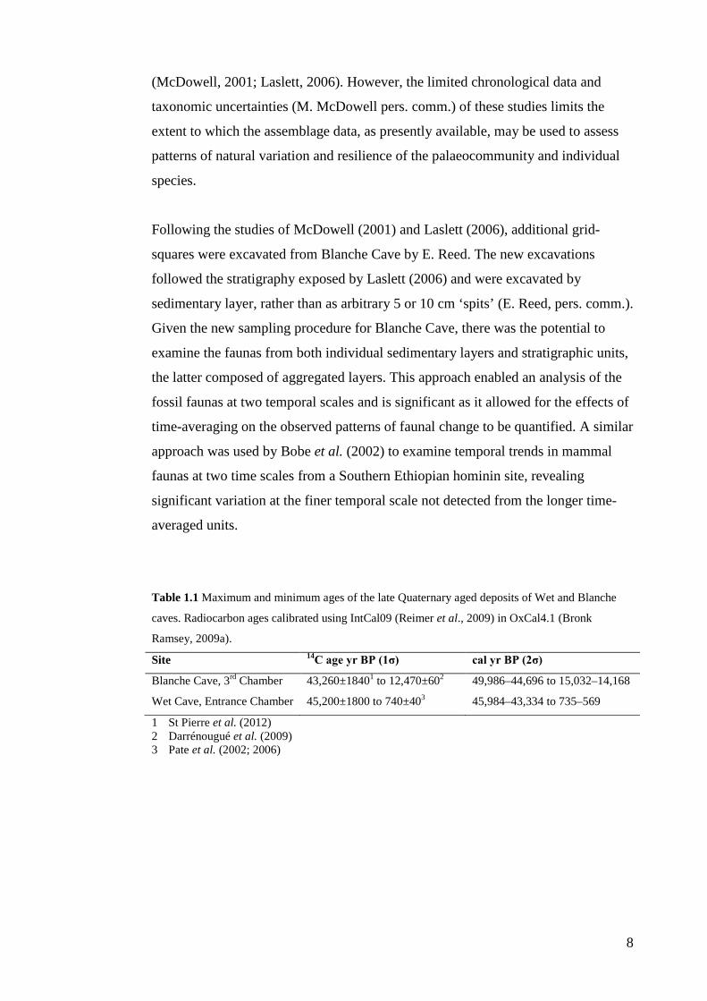
Table 1.1 Maximum and minimum ages of the late Quaternary aged deposits of Wet and Blanche
caves. Radiocarbon ages calibrated using IntCal09 (Reimer et al., 2009) in OxCal4.1 (Bronk
Ramsey, 2009a). Site 14C age yr BP (1σ) cal yr BP (2σ)
Blanche Cave, 3rd Chamber 43,260±18401 to 12,470±602 49,986–44,696 to 15,032–14,168
Wet Cave, Entrance Chamber 45,200±1800 to 740±403 45,984–43,334 to 735–569
1 St Pierre et al. (2012) 2 Darrénougué et al. (2009) 3 Pate et al. (2002; 2006)
9
Aims The aim of research presented in this thesis was to determine the magnitude and
ecological extent of variation (or stability) expressed by the small mammal
palaeocommunity of south-eastern South Australia through the last glacial cycle and
to examine if such variation occurred within extrinsic and intrinsic thresholds. More
specifically, it aimed to:
1. Determine the magnitude of natural variation of the small mammal
palaeocommunity and individual species through the last glacial cycle
across the following attributes: species richness, evenness, composition,
rank-order abundance and the relative abundance of individual species.
2. Identify thresholds of resilience of the small mammal palaeocommunity
through the last glacial cycle relating to the following factors:
a. Intrinsic: palaeocommunity composition, rank-order abundance and
species abundances, and
b. Extrinsic: sea-surface temperature, effective moisture availability
and local vegetation types.
3. Examine how sampling variation within and between sites and temporal
resolution influenced the patterns of variation and/or stability observed in
the small mammal fossil assemblages.
Supporting objectives A series of supporting aims and objectives associated with establishing the
chronological and depositional contexts of the study deposits were critical to
achieving the overall aims of the thesis.
The greater chronological control, finer temporal resolution and more adequate and
quantitative faunal sampling in the studies of Prideaux et al. (2007) and Macken et
al. (2012) were fundamental in revealing the faunal changes that were previously
obscured by poor sampling in studies of the Naracoorte Cave faunas (Moriarty et
10
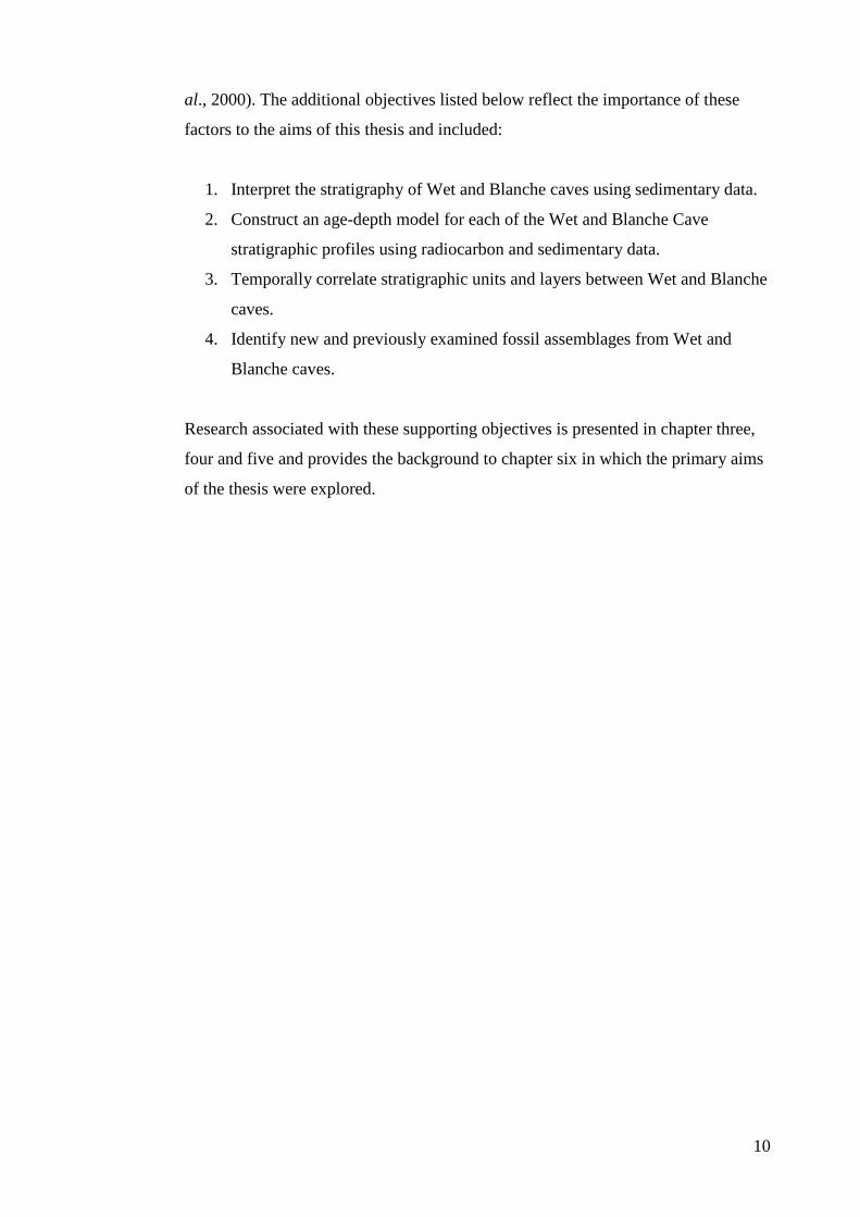
al., 2000). The additional objectives listed below reflect the importance of these
factors to the aims of this thesis and included:
1. Interpret the stratigraphy of Wet and Blanche caves using sedimentary data.
2. Construct an age-depth model for each of the Wet and Blanche Cave
stratigraphic profiles using radiocarbon and sedimentary data.
3. Temporally correlate stratigraphic units and layers between Wet and Blanche
caves.
4. Identify new and previously examined fossil assemblages from Wet and
Blanche caves.
Research associated with these supporting objectives is presented in chapter three,
four and five and provides the background to chapter six in which the primary aims
of the thesis were explored.
11
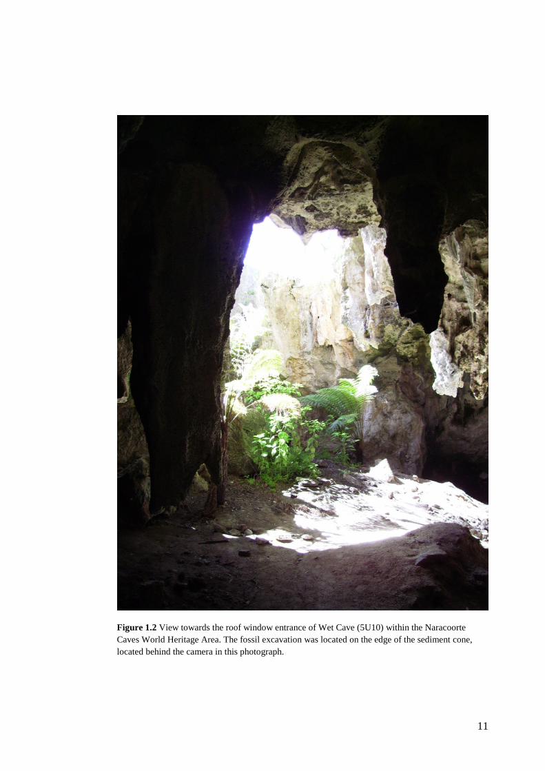
Figure 1.2 View towards the roof window entrance of Wet Cave (5U10) within the Naracoorte Caves World Heritage Area. The fossil excavation was located on the edge of the sediment cone, located behind the camera in this photograph.
12
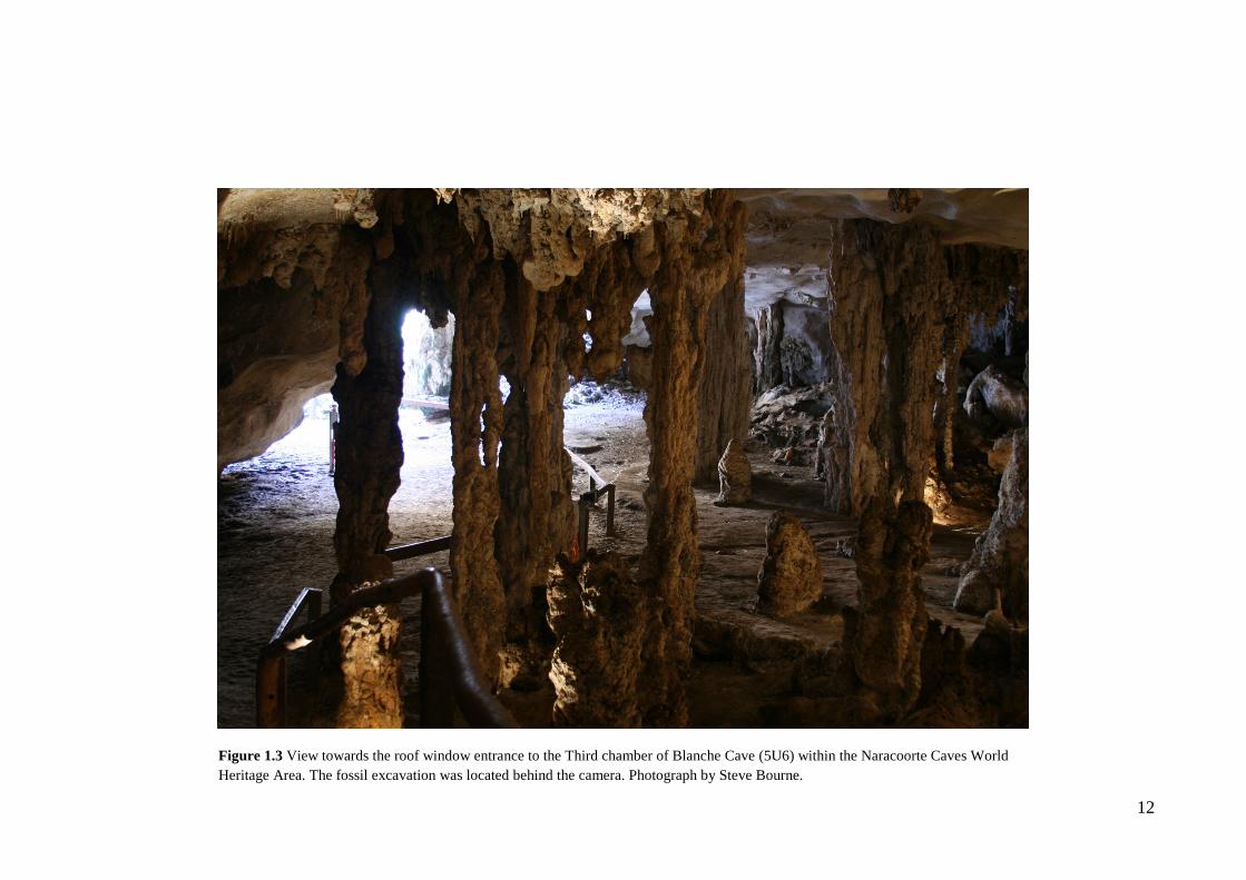
Figure 1.3 View towards the roof window entrance to the Third chamber of Blanche Cave (5U6) within the Naracoorte Caves World Heritage Area. The fossil excavation was located behind the camera. Photograph by Steve Bourne.
13
Thesis Structure
Introduction to the literature review In the literature review, I examine the significance of managing for natural variation
in biodiversity conservation, particularly in light of climate change effects on
species and communities. Given the strong argument presented in ecological and
palaeoecological literature for long-term studies of ecosystems, I also explore the
methods used to measure and describe faunal change (variability) in long-term data.
Of particular relevance to my study of the Naracoorte small mammal faunas was
how the techniques used to measure faunal responses and community variability in
fossil assemblages, and the biological and metric scale of study, can affect the
statistical and inferred ecological significance of observed patterns (e.g., Rahel,
1990; Schopf and Ivany, 1998; Hadly and Barnosky, 2009). Examination of these
issues in the review informed the approach I used to measure, define and interpret
variability, and hence, resilience of the Late Quaternary small mammal faunas of
the NCWHA.
Introduction to the research chapters, style and progression Research conducted for this thesis is presented in manuscript format, with chapters
composed of published papers and submitted manuscripts. As a result, some
information is repeated through the thesis, such as descriptions of the study locality,
a required element for each individual manuscript.
Where a research chapter has been published, a citation to the paper is provided but
the manuscript itself is presented in a format and style consistent with the thesis in
order to facilitate ease of reading the thesis as a whole. However, there are some
inconsistencies with the use and style of some terminology between chapters. For
example, ‘Late Pleistocene’ is interchangeable with both ‘late Pleistocene’ and
‘Upper Pleistocene.’ ‘Middle Pleistocene’ is also referred to as ‘middle
Pleistocene’, while ‘Early Pleistocene’ is interchangeable with ‘early Pleistocene’
and ‘Lower Pleistocene’. These terms were used in accordance with directions from
the Journal editors associated with each of the published manuscripts. Additionally,
the prefix ‘palaeo’ is spelt using American English (‘paleo’) in chapter three, in
accordance with the style requested by the editor of The Australian Journal of Earth
14
Science. All chronological data are presented as calibrated calendar years before
present (yr BP), unless otherwise stated.
References for each chapter and appendix are compiled at the end of the thesis to
reduce repetition and the size of the thesis. Referencing style varies amongst the
sections of the thesis as they were published by, or prepared for, different journals;
however, all references are formatted to the same style in the bibliography at the
end of the thesis.
As all manuscripts have multiple authors, a summary of the contribution of each
author to the work has been provided. All co-authors have given permission for the
relevant manuscripts to be included in the thesis as indicated by their signatures on
the coversheet for each research chapter. In some cases, co-authors could not
provide a signature (due to field work or other travel commitments). In those cases,
their names have been typed and a copy of their authorisation by email has been
kept for reference.
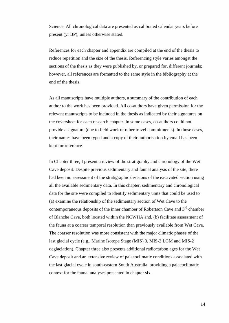
In Chapter three, I present a review of the stratigraphy and chronology of the Wet
Cave deposit. Despite previous sedimentary and faunal analysis of the site, there
had been no assessment of the stratigraphic divisions of the excavated section using
all the available sedimentary data. In this chapter, sedimentary and chronological
data for the site were compiled to identify sedimentary units that could be used to
(a) examine the relationship of the sedimentary section of Wet Cave to the
contemporaneous deposits of the inner chamber of Robertson Cave and 3rd chamber
of Blanche Cave, both located within the NCWHA and, (b) facilitate assessment of
the fauna at a coarser temporal resolution than previously available from Wet Cave.
The coarser resolution was more consistent with the major climatic phases of the
last glacial cycle (e.g., Marine Isotope Stage (MIS) 3, MIS-2 LGM and MIS-2
deglaciation). Chapter three also presents additional radiocarbon ages for the Wet
Cave deposit and an extensive review of palaeoclimatic conditions associated with
the last glacial cycle in south-eastern South Australia, providing a palaeoclimatic
context for the faunal analyses presented in chapter six.

15
Chapter four presents a Bayesian age-depth model-based analysis of the
stratigraphic and chronological contexts of Wet and Blanche Caves. The age models
developed for Wet and Blanche caves provided not only a robust assessment of the
ages of all stratigraphic layers/units within the sites, but enabled them to be
statistically correlated. Using the age-models, we were able to define two temporal
scales for analysis of the fossil assemblages (a macroscale and a mesoscale). The
coarser macroscale was associated with major climatic phases of the last glacial
cycle (e.g., MIS-3, MIS-2 glacial maximum and MIS-2 deglaciation). The
mesoscale provided finer time-slices within each of these climatic phases. Without
the age models, the temporal correlation of the two sites would have been inferred
from the sediments and individually calibrated radiocarbon ages, without estimates
of statistical uncertainty which may have biased the comparative faunal analyses
and/or been inaccurate.
Chapter five introduces the small mammal taxa identified from the study sites and
the methodology used to sample the fossil assemblages. The biogeographic
implications of the fossil records of the Naracoorte Caves are also discussed in this
chapter, highlighting the need for greater communication of fossil occurrences to
enhance knowledge of the past distribution of mammal faunas prior to European
arrival in Australia. As 47 species were identified in this project, systematic
palaeontology is presented in Appendix D only for species of Dasyuridae
previously unrecorded from the NCWHA and/or the Late Pleistocene–Holocene
from this locality. Limiting the systematic palaeontology to this selection of the
fauna aims to demonstrate how I identified the fauna without eclipsing the thesis
with a lengthy descriptive chapter or providing descriptions for taxa that are well
described elsewhere. Appendix D also contains a list of references used to aid in the
identification of species from other families. In the published manuscript systematic
palaeontology was provided for the two unidentified taxa, Dasyuridae sp. 1 and
Sminthopsis sp. 1 to alert other researchers to the potential of new taxa, or
specimens that present morphologically variants of known taxa within the fossil
assemblages of the Naracoorte Caves.
In chapter six, a quantitative analysis of the fossil assemblages of Wet and Blanche
Cave is presented, directly addressing the aims of the thesis. The analyses in chapter
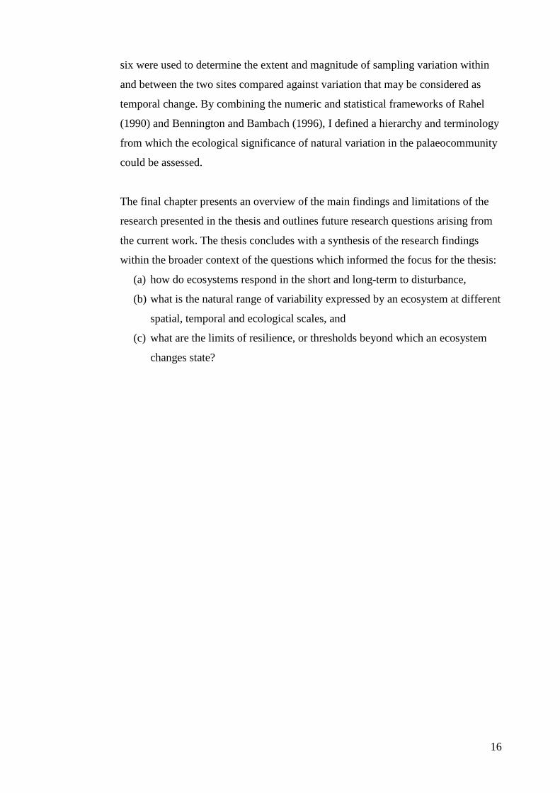
16
six were used to determine the extent and magnitude of sampling variation within
and between the two sites compared against variation that may be considered as
temporal change. By combining the numeric and statistical frameworks of Rahel
(1990) and Bennington and Bambach (1996), I defined a hierarchy and terminology
from which the ecological significance of natural variation in the palaeocommunity
could be assessed.
The final chapter presents an overview of the main findings and limitations of the
research presented in the thesis and outlines future research questions arising from
the current work. The thesis concludes with a synthesis of the research findings
within the broader context of the questions which informed the focus for the thesis:
(a) how do ecosystems respond in the short and long-term to disturbance,
(b) what is the natural range of variability expressed by an ecosystem at different
spatial, temporal and ecological scales, and
(c) what are the limits of resilience, or thresholds beyond which an ecosystem
changes state?
17
2. Literature Review
Natural variation in (palaeo)ecological assemblages: scale,
measurement and interpretation.
“We get closer to understanding the whole by considering its parts at more than one
scale.” Schopf and Ivany, 1998, p. 187.
Introduction
Climate change: biodiversity adaptation and resilience The effects of climate change on organisms, communities and ecosystems are of
concern to biodiversity managers and are expected to include shifts in the
distribution and abundance of species and changes to population, life history and
reproductive dynamics (e.g., Williams et al., 2003; Meyeneck, 2004; Preston et al.,
2008; Marini et al., 2009). As a result, climate change is expected to increase the
extinction risk of vulnerable taxa, facilitate the spread of invasive species and alter
the dynamics of ecological processes and interactions (e.g., Green et al., 2008;
Brennan et al., 2009; Kannan and James, 2009). Confounding climate change
effects are the consequences of human activities on biodiversity. Of concern in
Australia is the loss, fragmentation and degradation of habitat, depletion of natural
resources, inappropriate fire regimes and changes to aquatic environments and
water flows (NBSRTG, 2009).
In order to mediate the combined risks of climate change and anthropogenic
landscape disturbance, an emergent goal of biodiversity conservation is to develop
the adaptive capacity of ecological communities and populations. In the Australian
Biodiversity Conservation Strategy, this goal is defined within the context of
building ecosystem resilience (NBSRTG, 2009). At face value, these goals appear
to be contradictory; adaptation suggests change while resilience may be equated
with stability. However, as defined by Walker et al. (2004), ecosystem resilience
refers to the “capacity of a system to absorb disturbance and reorganise while
undergoing change so as to retain essentially the same function, structure, identity
and feedbacks” (p.1). The latter aspect is at the heart of most ecological definitions
18
of resilience, that is, how much pressure or change an ecological system can
withstand before it shifts to a new, alternative steady-state (Holling, 1996; Walker
et al., 2009). It is perhaps through the recognition that variation in ecosystem
components can contribute to overall ecosystem stability that concepts of adaptation
and resilience may be integrated (Cumming et al., 2005). However, from a
biodiversity conservation perspective, it may not be most critical to quantify
resilience per se, but instead to develop a greater understanding of the type, drivers
and consequences of variation in ecological systems and communities. For example,
it may be more useful to have information about thresholds that operate within
systems that when crossed, lead to new ecosystem states, as well as baselines
against which such changes may be compared (Hadly and Barnosky, 2009; Dietl
and Flessa, 2011).
Although there is an urgency for appropriate biodiversity conservation strategies,
addressing questions about variability and resilience is limited by a lack of
knowledge about (a) how ecosystems respond in the short and long-term to
disturbance (including climate change) (Lepetz et al., 2009), (b) the natural range of
variability expressed by an ecosystem at different spatial, temporal and ecological
scales (Landres et al., 1999) and (c) the limits of resilience, or thresholds beyond
which an ecosystem changes state (Willis et al., 2005; 2007; 2010; NBSRTG,
2009).
To address these questions, long-term studies of ecosystems, in particular, those
covering temporal scales sufficient to detect the full extent of ecosystem
reorganisation following climatic change and other disturbances, are required. Yet
few studies cover temporal scales that are sufficient to detect the full extent of
ecosystem reorganisation following disturbance (Van Valkenburgh, 1995; Lepetz et
al., 2009). In the absence of long-term data, bioclimatic models have become an
important tool in biodiversity management planning. These have been used
extensively for predicting the effects of future climate change on species
distributions and abundance (e.g., Williams et al., 2003; Shoo et al., 2005);
although, there are limitations to the scope, detail and accuracy of modelled
responses (Pearson and Dawson, 2003; Willis and Bhagwat, 2009). Extensive
habitat fragmentation, species loss and subsequent ecosystem disruption also limits
19
our ability to understand patterns of natural variation and the interaction of
ecosystem changes with the long-term persistence or loss of different ecosystem
attributes over time (Magurran and Henderson, 2010).
Palaeoecology and biodiversity conservation Palaeoecological studies are increasingly recognised as a valuable source of
empirical data on past ecosystems (e.g., Willis et al., 2005; MacDonald et al., 2008;
Hadly and Barnosky, 2009; Willis et al., 2010), with many examples of the use of
“natural archives” (Smol, 2010) to contextualise current and future landscape
changes (e.g., Barnosky and Shabel, 2005; Saunders and Taffs, 2009; Bellingham et
al., 2010; Bilney et al., 2010; Carassco et al., 2010; Finney et al., 2010; Renberg et
al., 2010). These natural archives include biotic (e.g., bones, pollen, diatoms) and
abiotic (e.g., speleothem cave formations, stable isotopes) records that can be used
to reconstruct past environments and empirically test the history of life and models
of global change (e.g., Barnosky et al., 2003; Willis et al., 2005; MacDonald et al.,
2008).
As shown by Willis et al. (2010), the application of palaeoecological archives to
modern conservation and management problems are broad in type, scale and value
and can include (a) informing predictions about climate change responses and
thresholds based on past ecological and climatic variability, (b) identifying the
combinations of biotic and abiotic processes that most contributed to past ecological
resilience and where these are likely to occur under future climate change scenarios,
and (c) providing insights on novel, or non-analogous communities and their
management. These applications go some way to addressing the three deficiencies
in knowledge identified above: that is, understanding how ecosystems respond to
disturbance at different time-scales, the range of variation and types of states that
may normally be expressed by different systems under different environmental and
climatic scenarios and finally, the thresholds operating within systems that define
the limits or boundaries of these states and ultimately, ecosystem resilience.
Of particular interest for this review is not necessarily what palaeoecological
records reveal about natural variation and resilience in past ecological systems, but
rather how natural variation and resilience are measured and defined. More
20
specifically, the literature review examines how temporal, spatial and taxonomic
scales and sampling effects can influence patterns detected in palaeoecological
deposits. Ultimately, such issues affect how palaeoecological trends are compared
against changes observed in modern systems and the inferred ecological
significance of such changes (Bennington et al., 2009).
The literature review is divided into three sections, with the first providing an
overview of the geological setting, chronology, faunas, climate and environmental
context the vertebrate fossil assemblages of the NCWHA, the study locality. In the
second section, particular attention is given to the techniques, results and
implications of faunal change observed in the Naracoorte Cave record through time
to (a) show how the aims of the thesis have been informed by the findings of past
research from this locality, and (b) highlight key sampling issues that can influence
patterns of faunal change observed in fossil records and which were considered in
the design of the research presented in the thesis.
The final section re-focusses on natural variation and resilience in ecological
systems. This section explores how natural variation and resilience have been
inferred from faunal changes observed in palaeoecological assemblages, including
those of the NCWHA. It also focusses on hierarchical relationships across common
metrics used to examine change in fossil assemblages (species richness,
composition and abundance) and the biodiversity conservation implications of
variation across these metrics. This section of the review aims to complement Hadly
and Barnosky (2009) who explored key mechanisms by which vertebrate fossil
records contribute knowledge about natural variation in ecosystems.
21
Fossil deposits of the Naracoorte Caves World Heritage Area
Scientific and natural history values The fossil deposits of the Naracoorte Caves contain the first dated Middle
Pleistocene bone assemblages in Australia (Ayliffe et al., 1998; Prideaux, 2006).
They also provide records of the Late Pleistocene and Holocene, a period not well
represented in other Australian vertebrate fossil deposits (Prideaux, 2006). In
recognition of their natural and scientific value, the Naracoorte Cave fossil deposits
were inscribed to the World Heritage List in 1994. Together with Riversleigh in
Queensland, they are listed as the Australian Fossil Mammal Sites. There are 26
known caves within the NCWHA, containing nearly 100 fossil sites, each
representing a snapshot of past environments and faunas of the region (Reed and
Bourne, 2000, 2009). Over their c. 500,000 year accumulation history, the caves
have acted as pitfall traps and predator dens, preserving a record of faunal diversity
and abundance over time.
The potential of the Naracoorte Caves to provide a long-term record of faunal
response to climate change was recognised from the earliest scientific exploration
of the caves (Wells, 1975; Wells et al., 1984). As research has expanded knowledge
of the temporal distribution, diversity and richness of the fossil deposits, three key
advantages for researching fauna and climate from the caves have emerged: (a) the
ability to track mammal diversity change over multiple climatic cycles at one
geographic location (e.g., Prideaux et al., 2007; Macken et al., 2012) (b) the ability
to test models of mammal response to climate change across multiple sites of the
same age (e.g., McDowell, 2001) and (c) enable the influence of taphonomic and
accumulation biases on the fidelity of the palaeontological record to the sampled
community to be determined (e.g., Reed, 2003; Fraser and Wells, 2006).
In their recent review of the effects of climate change on biological systems over
the Cainozoic, Blois and Hadly (2009) identified that palaeoecological studies
integrating climatic, environmental and community patterns are required if such
data is to be used to model and predict habitat and species changes in the future.
The Naracoorte Caves facilitate such integrated studies as they contain deep
sediment deposits, abundant speleothems and other natural archives in addition to
bones such as fossil pollen (Darrénougué et al., 2009).
22
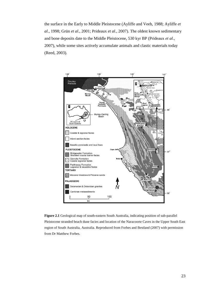
Geological Context The NCWHA is located in south-eastern South Australia, c. 12 km from the
township of Naracoorte (37°0’S, 149°48’E; Fig.1.1). The caves lie within an
uplifted portion of the Oligocene to Miocene aged Gambier Limestone, a deep
fossiliferous limestone of marine sediment origins (Ludbrook, 1961; Li et al.,
2000). Overlying this sequence is a series of sub-parallel, stranded Pleistocene
beach dune facies that extend from Naracoorte to the coast at Robe (Sprigg, 1952,
Murray-Wallace et al., 2001; Fig. 2.1). The oldest and easternmost of these dunes,
the Naracoorte East Ridge, was deposited greater than 780 kyr BP and may be as
old as 935 kyr BP (Murray-Wallace et al., 2001). These ridges are composed of
bioclastic, calcareous carbonates of the Bridgewater formation, intermittently
overlain by dune sands and calcrete (Belperio, 1995).
The prevailing model of cave formation that informed the first palaeontological
studies of the caves was based on phreatic dissolution of fallen roof blocks of the
Gambier Limestone over the late Miocene/early Pliocene (Wells et al., 1984). More
recent investigation suggests that movement of the Kanawinka fault uplifted the
Gambier Limestone underneath the East Naracoorte Ridge, facilitating cave
formation by controlling the development and distribution of joints within the
limestone (Lewis et al., 2006).
The development of entrances from the surface into the caves was determined by
Reed (2003) based on an extensive survey of caves in the NCWHA and the South
East region. Narrow ‘solution pipe’ openings, up to a maximum of 1.8 m diameter,
formed as a result of secondary dissolution of limestone via vadose flow along
vertical joints and subsequent lateral enlargement. These entrances contrast with
much larger roof ‘windows,’ which reach up to 13.7 m diameter. Such roof window
entrances formed following collapse of thin limestone above domed chambers
(Reed, 2003).
Accumulation of vertebrate bone material and clastic sediments in the caves has
been constrained by the opening, and in the case of solution pipes, closing of these
cave entrances over time (Reed, 2003). Dating of clastic sediments, bone material
and speleothem cave formations indicates that the Naracoorte caves first opened to
23
the surface in the Early to Middle Pleistocene (Ayliffe and Veeh, 1988; Ayliffe et
al., 1998; Grün et al., 2001; Prideaux et al., 2007). The oldest known sedimentary
and bone deposits date to the Middle Pleistocene, 530 kyr BP (Prideaux et al.,
2007), while some sites actively accumulate animals and clastic materials today
(Reed, 2003).
Figure 2.1 Geological map of south-eastern South Australia, indicating position of sub-parallel
Pleistocene stranded beach dune facies and location of the Naracoorte Caves in the Upper South East
region of South Australia, Australia. Reproduced from Forbes and Bestland (2007) with permission
from Dr Matthew Forbes.

24
Palaeontological Research
Early exploration and study of the fossil deposits within the NCWHA has been
reviewed previously (McDowell, 2001; Reed, 2003). Therefore, this section
presents an overview of more recent palaeontological research at the caves since the
1969 discovery of Main Fossil Chamber in Victoria Fossil Cave.
Chronology
Cave deposits such as those of the NCWHA provide the richest source of
Pleistocene faunal remains in Australia (Wells, 1978). However, as a result of their
complex accumulation histories, cave deposits are considered to be less than ideal
for palaeontological studies (Lowe and Walker, 1997; Forbes et al., 2007).
Attempts to date the Main Fossil Chamber deposit in Victoria Fossil Cave (VFC)
reflect the challenges of dating cave deposits (Wells et al., 1984; Ayliffe and Veeh,
1988; Grün et al., 2001); however, research into other deposits of the NCWHA has
yielded valuable palaeontological information within more tightly resolved
temporal contexts (Fig. 2.2 and references therein). This has been facilitated by
advances in dating techniques and the presence of multiple datable materials in the
deposits such as cave speleothems (flowstones, stalagmites, stalactites and straws),
quartz-bearing sediments, charcoal, bones and teeth.
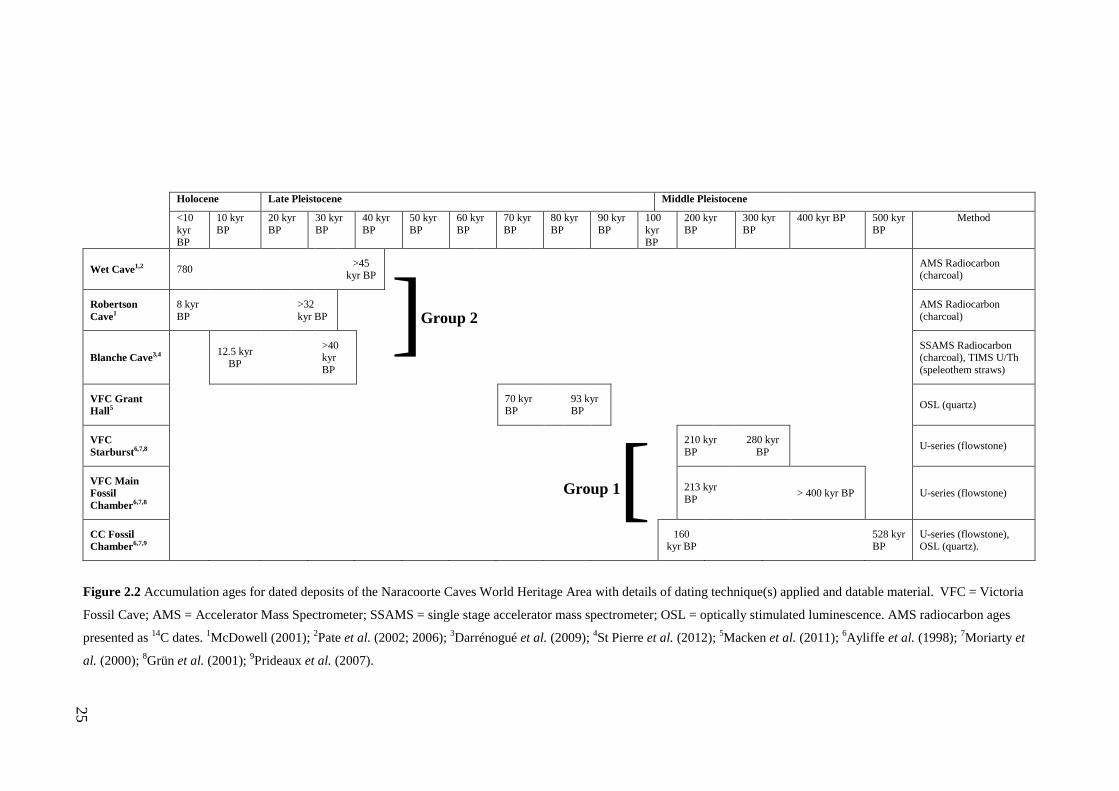
The accumulation ages for the deposits listed in Fig. 2.2 indicate that at least three
sites accumulated material over the same time intervals of the Middle (Group 1
deposits) and Late Pleistocene (Group 2 deposits) within the NCWHA. Only the
Grant Hall deposit represents a time not captured by any other known deposit
(Ayliffe and Veeh, 1988; Macken et al., 2011). The age distribution of the NCWHA
deposits provides the opportunity to examine faunal change over multiple climatic
cycles at one geographic location, test models of mammal response to climate
change across multiple sites of the same age and understand how taphonomic and
accumulation biases influence the fidelity of the palaeontological record with the
sampled community.
25
Holocene Late Pleistocene Middle Pleistocene
<10 kyr BP
10 kyr BP
20 kyr BP
30 kyr BP
40 kyr BP
50 kyr BP
60 kyr BP
70 kyr BP
80 kyr BP
90 kyr BP
100 kyr BP
200 kyr BP
300 kyr BP
400 kyr BP 500 kyr BP
Method
Wet Cave1,2 780 >45 kyr BP AMS Radiocarbon
(charcoal)
Robertson Cave1
8 kyr BP >32
kyr BP
AMS Radiocarbon (charcoal)
Blanche Cave3,4 12.5 kyr BP
>40 kyr BP
SSAMS Radiocarbon (charcoal), TIMS U/Th (speleothem straws)
VFC Grant Hall5 70 kyr
BP 93 kyr BP
OSL (quartz)
VFC Starburst6,7,8 210 kyr
BP 280 kyr
BP U-series (flowstone)
VFC Main Fossil Chamber6,7,8
213 kyr BP > 400 kyr BP U-series (flowstone)
CC Fossil Chamber6,7,9 160
kyr BP 528 kyr BP
U-series (flowstone), OSL (quartz).
Figure 2.2 Accumulation ages for dated deposits of the Naracoorte Caves World Heritage Area with details of dating technique(s) applied and datable material. VFC = Victoria
Fossil Cave; AMS = Accelerator Mass Spectrometer; SSAMS = single stage accelerator mass spectrometer; OSL = optically stimulated luminescence. AMS radiocarbon ages
presented as 14C dates. 1McDowell (2001); 2Pate et al. (2002; 2006); 3Darrénogué et al. (2009); 4St Pierre et al. (2012); 5Macken et al. (2011); 6Ayliffe et al. (1998); 7Moriarty et
al. (2000); 8Grün et al. (2001); 9Prideaux et al. (2007).
Group 2 ]
[ Group 1
26
Sediments and Stratigraphy
Defining the stratigraphic and sedimentological context of fossil deposits is an
important prerequisite to their excavation and interpretation. The first sediment
analyses from the NCWHA were of the clastic infills of Main Fossil Chamber,
Victoria Fossil Cave (Wells et al., 1984) and analyses have now been conducted on
other bone-bearing deposits (e.g., Moriarty et al., 2000; McDowell, 2001; Laslett,
2006; Forbes and Bestland, 2007; Forbes et al., 2007; Prideaux et al., 2007;
Darrénougué et al., 2009; Macken et al., 2011). Typical sediment types found in the
caves range from homogenous yellow sands (e.g., middle unit of Robertson Cave;
Forbes et al., 2007) to organic rich, brown silty sands (e.g., Unit 2 of Blanche Cave;
Darrénougué et al., 2009) and reddish silts (e.g., Grant Hall; Macken, 2009; Macken et
al., 2011) as originally described by Forbes and Bestland (2007).
Transport and deposition of clastic sediments into the caves has occurred largely via
wind and water action, producing sedimentary cones and fans with unique stratigraphic
and physical characteristics. The mode and rate of sediment transport and resulting
sediment profiles within the caves is influenced by a wide range of factors. These
include:
(a) Surface conditions such as vegetation and soil cover which control the rate of
water flow and therefore rates of accumulation (Wells et al., 1984).
(b) The presence and size of dolines (shallow depressions) in the limestone
bedrock above the cave entrance which may concentrate sediments and
organic matter via run-off flows prior to deposition into the chambers below.
Moriarty et al. (2000) suggested this as the primary mode of accumulation of
sediments into the caves at Naracoorte, implying discrete, bulk depositional
episodes in the past resulting in aggraded stratigraphic layers in the deposit.
(c) Cave entrance type and size, which influences the nature of the sedimentary
cone and rates of accumulation over time. In caves with large roof windows,
the sediment cone is typically composed of limestone debris and is built up
over time by clastic and organic material inputs (Reed, 2003). In many of
these caves, plants, fungi and algae grow within the light zone over the
sedimentary cone (Reed, 2003). In contrast, smaller solution pipe entrances
may block up over time as the sediment cone fills the pipe. Large water inputs
27
may cause mass slumping events and distal transport of sediments, re-opening
the solution pipe.
(d) Within-cave processes such as water transport, slumping, saturated mud flows
and animal movements, which can lead to secondary deposition and erosion
across sedimentary cones and fans. These processes produce unique
stratigraphic features including deep scours, cut and fill structures and flames
(e.g., McDowell, 2001).
Fauna
Taphonomy and accumulation
The first extensive taphonomic investigation of fossil deposits of the NCWHA was
conducted by Reed (2003). This work focused on the large mammal bone material of
the Main Fossil Chamber, Victoria Fossil Cave and included neo-taphonomic
observations in caves acting as contemporary pitfall traps. Reed (2003) documented
the range of physical and biological factors influencing pitfall entrapment in the
Naracoorte Caves, including cave entrance dynamics, animal locomotion and
behaviour.
Reed (2003) showed that pitfall entrapment, or ‘pitfall mortality’ produces a near
random sample of the mammal community through cumulative accretion over time. By
comparison, roof window deposits record a more diverse species assemblage, resulting
in higher fidelity to the actual composition of the palaeocommunity that was sampled
in the deposit. This occurs largely as a result of taphonomic biases associated with the
cave entrance type. Solution pipes bias entrapment of saltatorial species while roof
windows captured a more equal representation of faunas with different movement
habits (i.e., saltatorial, scansorial and arboreal). This occurs as roof windows facilitate
a combination of pitfall entrapment, predator accumulation and within-cave habitation
(Reed, 2003).
In the Naracoorte fossil sites, Barn and Masked Owl (Tyto alba and Tyto
novaehollandiae) are the main predatory accumulating agents; although, mammalian
carnivores may be responsible for some deposits (Reed and Bourne, 2000). The Late
Pleistocene fossil assemblages of the Group 2 deposits are predominantly owl pellet
derived (McDowell, 2001; Laslett, 2006). These assemblages are dominated by small
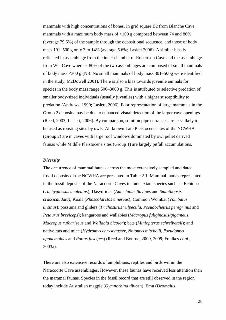
28
mammals with high concentrations of bones. In grid square B2 from Blanche Cave,
mammals with a maximum body mass of <100 g composed between 74 and 86%
(average 79.6%) of the sample through the depositional sequence, and those of body
mass 101–500 g only 3 to 14% (average 6.6%; Laslett 2006). A similar bias is
reflected in assemblage from the inner chamber of Robertson Cave and the assemblage
from Wet Cave where c. 80% of the two assemblages are composed of small mammals
of body mass <300 g (NB. No small mammals of body mass 301–500g were identified
in the study; McDowell 2001). There is also a bias towards juvenile animals for
species in the body mass range 500–3000 g. This is attributed to selective predation of
smaller body-sized individuals (usually juveniles) with a higher susceptibility to
predation (Andrews, 1990; Laslett, 2006). Poor representation of large mammals in the
Group 2 deposits may be due to enhanced visual detection of the larger cave openings
(Reed, 2003; Laslett, 2006). By comparison, solution pipe entrances are less likely to
be used as roosting sites by owls. All known Late Pleistocene sites of the NCWHA
(Group 2) are in caves with large roof windows dominated by owl pellet derived
faunas while Middle Pleistocene sites (Group 1) are largely pitfall accumulations.
Diversity
The occurrence of mammal faunas across the most extensively sampled and dated
fossil deposits of the NCWHA are presented in Table 2.1. Mammal faunas represented
in the fossil deposits of the Naracoorte Caves include extant species such as: Echidna
(Tachyglossus aculeatus); Dasyuridae (Antechinus flavipes and Sminthopsis
crassicaudata); Koala (Phascolarctos cinereus); Common Wombat (Vombatus
ursinus); possums and gliders (Trichosurus vulpecula, Pseudocheirus peregrinus and
Petaurus breviceps); kangaroos and wallabies (Macropus fuliginosus/giganteus,
Macropus rufogriseus and Wallabia bicolor); bats (Miniopterus schreibersii); and
native rats and mice (Hydromys chrysogaster, Notomys mitchelli, Pseudomys
apodemoides and Rattus fuscipes) (Reed and Bourne, 2000, 2009; Foulkes et al.,
2003a).
There are also extensive records of amphibians, reptiles and birds within the
Naracoorte Cave assemblages. However, these faunas have received less attention than
the mammal faunas. Species in the fossil record that are still observed in the region
today include Australian magpie (Gymnorhina tibicen), Emu (Dromaius
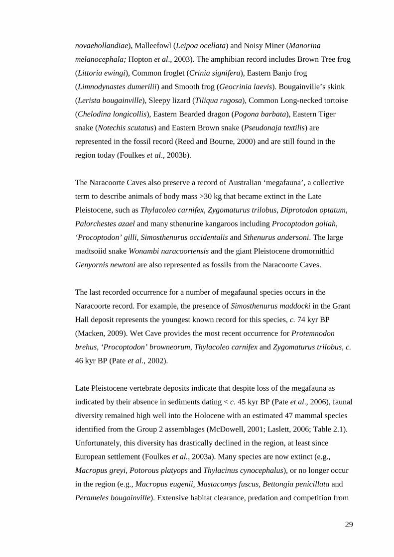
29
novaehollandiae), Malleefowl (Leipoa ocellata) and Noisy Miner (Manorina
melanocephala; Hopton et al., 2003). The amphibian record includes Brown Tree frog
(Littoria ewingi), Common froglet (Crinia signifera), Eastern Banjo frog
(Limnodynastes dumerilii) and Smooth frog (Geocrinia laevis). Bougainville’s skink
(Lerista bougainville), Sleepy lizard (Tiliqua rugosa), Common Long-necked tortoise
(Chelodina longicollis), Eastern Bearded dragon (Pogona barbata), Eastern Tiger
snake (Notechis scutatus) and Eastern Brown snake (Pseudonaja textilis) are
represented in the fossil record (Reed and Bourne, 2000) and are still found in the
region today (Foulkes et al., 2003b).
The Naracoorte Caves also preserve a record of Australian ‘megafauna’, a collective
term to describe animals of body mass >30 kg that became extinct in the Late
Pleistocene, such as Thylacoleo carnifex, Zygomaturus trilobus, Diprotodon optatum,
Palorchestes azael and many sthenurine kangaroos including Procoptodon goliah,
‘Procoptodon’ gilli, Simosthenurus occidentalis and Sthenurus andersoni. The large
madtsoiid snake Wonambi naracoortensis and the giant Pleistocene dromornithid
Genyornis newtoni are also represented as fossils from the Naracoorte Caves.
The last recorded occurrence for a number of megafaunal species occurs in the
Naracoorte record. For example, the presence of Simosthenurus maddocki in the Grant
Hall deposit represents the youngest known record for this species, c. 74 kyr BP
(Macken, 2009). Wet Cave provides the most recent occurrence for Protemnodon
brehus, ‘Procoptodon’ browneorum, Thylacoleo carnifex and Zygomaturus trilobus, c.
46 kyr BP (Pate et al., 2002).
Late Pleistocene vertebrate deposits indicate that despite loss of the megafauna as
indicated by their absence in sediments dating < c. 45 kyr BP (Pate et al., 2006), faunal
diversity remained high well into the Holocene with an estimated 47 mammal species
identified from the Group 2 assemblages (McDowell, 2001; Laslett, 2006; Table 2.1).
Unfortunately, this diversity has drastically declined in the region, at least since
European settlement (Foulkes et al., 2003a). Many species are now extinct (e.g.,
Macropus greyi, Potorous platyops and Thylacinus cynocephalus), or no longer occur
in the region (e.g., Macropus eugenii, Mastacomys fuscus, Bettongia penicillata and
Perameles bougainville). Extensive habitat clearance, predation and competition from

30
introduced species have contributed to the loss of these species. According to the 2001
Naracoorte Caves National Park Management Plan (SERNPWSA, 2001), 26 native
mammal species, 90 native birds and 27 species of reptiles persist in the Naracoorte
Caves National Park at the present time. Many of these extant species are considered
rare or endangered as a result of human modification to the landscape.
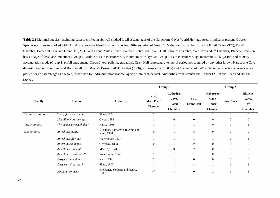
31
Table 2.1 Mammal species (excluding bats) identified in six well-studied fossil assemblages of the Naracoorte Caves World Heritage Area. 1 indicates present, 0 absent.
Species occurrences marked with cf. indicate tentative identification of species. Differentiation of Group 1 (Main Fossil Chamber, Victoria Fossil Cave (VFC); Fossil
Chamber, Cathedral Cave and Grant Hall, VFC) and Group 2 sites (Inner Chamber, Robertson Cave; 5U10 Entrance Chamber, Wet Cave and 3rd Chamber, Blanche Cave) on
basis of age of fossil accumulations (Group 1: Middle to Late Pleistocene, c. minimum of 74 kyr BP; Group 2: Late Pleistocene, age maximum c. 45 kyr BP) and primary
accumulation mode (Group 1: pitfall entrapment; Group 2: owl pellet aggradation). Grant Hall represents a temporal period not captured by any other known Naracoorte Cave
deposit. Sourced from Reed and Bourne (2000; 2009); McDowell (2001); Laslett (2006); Prideaux et al. (2007a) and Macken et al. (2012). Note that species occurrences are
plotted for an assemblage as a whole, rather than for individual stratigraphic layers within each deposit. Authorities from Strahan and Conder (2007) and Reed and Bourne
(2000).
Group 1 Group 2
Family Species Authority
VFC,
Main Fossil
Chamber
Cathedral
Cave,
Fossil
Chamber
VFC,
Grant Hall
Robertson
Cave,
Inner
Chamber
Wet Cave
Blanche
Cave,
3rd
Chamber
TACHYGLOSSIDAE Tachyglossus aculeatus Shaw, 1792 1 1 1 1 0 0
Megalibgwilia ramsayi‡ Owen, 1884 1 0 0 0 0 0
THYLACINIDAE Thylacinus cynocephalus† Harris, 1808 1 1 1 0 1 1
DASYURIDAE Antechinus agilis* Dickman, Parnaby, Crowther and King, 1998 0 1 cf. 0 0 0
Antechinus flavipes Waterhouse, 1837 1 1 1 1 1 1
Antechinus minimus Geoffroy, 1803 0 1 cf. 0 0 0
Antechinus stuartii* Macleay, 1841 1 0 cf. 0 0 0
Antechinus swainsonii* Waterhouse, 1840 1 1 1 0 0 0
Dasyurus maculatus* Kerr, 1792 1 1 0 0 0 0
Dasyurus viverrinus* Shaw, 1800 1 1 1 1 1 1
Ningaui yvonneae* Kitchener, Stoddart and Henry, 1983 cf. 1 0 1 1 1
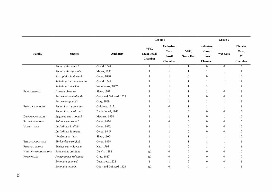
32
Group 1 Group 2
Family Species Authority
VFC,
Main Fossil
Chamber
Cathedral
Cave,
Fossil
Chamber
VFC,
Grant Hall
Robertson
Cave,
Inner
Chamber
Wet Cave
Blanche
Cave,
3rd
Chamber
Phascogale calura* Gould, 1844 1 1 1 0 0 0
Phascogale tapoatafa Meyer, 1893 1 1 1 1 1 1
Sarcophilus laniarius† Owen, 1838 1 1 0 0 1 0
Sminthopsis crassicaudata Gould, 1844 1 1 1 1 1 1
Sminthopsis murina Waterhouse, 1837 1 1 1 1 1 1
PERAMELIDAE Isoodon obesulus Shaw, 1787 1 1 1 1 0 1
Perameles bougainville* Quoy and Gaimard, 1824 1 1 1 0 0 1
Perameles gunnii* Gray, 1838 1 1 1 1 1 1
PHASCOLARCTIDAE Phascolarctos cinereus Goldfuss, 1817. 1 0 1 1 1 1
Phascolarctos stirtoni‡ Bartholomai, 1968 0 1 0 0 0 0
DIPROTODONTIDAE Zygomaturus trilobus‡ Macleay, 1858 1 1 1 0 1 0
PALORCHESTIDAE Palorchestes azael‡ Owen, 1874 1 0 0 0 0 0
VOMBATIDAE Lasiorhinus krefftii* Owen, 1872 1 1 0 0 0 0
Lasiorhinus latifrons* Owen, 1845 1 1 0 0 0 0
Vombatus ursinus Shaw, 1800 1 1 1 1 1 0
THYLACOLEONIDAE Thylacoleo carnifex‡ Owen, 1858 1 1 1 1 1 1
PHALANGERIDAE Trichosurus vulpecula Kerr, 1792 1 1 0 1 1 1
HYPSIPRYMNODONTIDAE Propleopus oscillans De Vis, 1888 cf. 0 0 0 0 0
POTOROIDAE Aepyprymnus rufescens Gray, 1837 cf. 0 0 0 0 0
Bettongia gaimardi Desmarest, 1822 1 1 0 0 0 1
Bettongia lesueur† Quoy and Gaimard, 1824 cf. 0 0 1 1 1
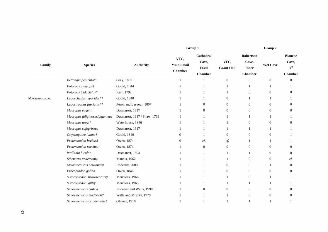
33
Group 1 Group 2
Family Species Authority
VFC,
Main Fossil
Chamber
Cathedral
Cave,
Fossil
Chamber
VFC,
Grant Hall
Robertson
Cave,
Inner
Chamber
Wet Cave
Blanche
Cave,
3rd
Chamber
Bettongia penicillata Gray, 1837 1 1 0 0 0 0
Potorous platyops† Gould, 1844 1 1 1 1 1 1
Potorous tridactylus* Kerr, 1792 1 1 1 0 0 0
MACROPODIDAE Lagorchestes leporides** Gould, 1840 1 1 0 1 1 1
Lagostrophus fasciatus** Péron and Lesueur, 1807 1 0 0 0 0 0
Macropus eugenii Desmarest, 1817 1 0 0 0 0 0
Macropus fuliginosus/giganteus Desmarest, 1817 / Shaw, 1789 1 1 1 1 1 1
Macropus greyi† Waterhouse, 1846 1 1 1 0 0 0
Macropus rufogriseus Desmarest, 1817 1 1 1 1 1 1
Onychogalea lunata† Gould, 1840 0 1 0 0 0 1
Protemnodon brehus‡ Owen, 1874 0 cf. cf. 1 1 1
Protemnodon roechus† Owen, 1874 1 0 0 0 0 0
Wallabia bicolor Desmarest, 1803 1 1 1 1 0 0
Sthenurus andersoni‡ Marcus, 1962 1 1 1 0 0 cf.
Metasthenurus newtonae‡ Prideaux, 2000 1 1 0 0 1 0
Procoptodon goliah Owen, 1846 1 1 0 0 0 0
‘Procoptodon' browneorum‡ Merrilees, 1968 1 1 1 0 1 1
‘Procoptodon' gilli‡ Merrilees, 1965 1 1 1 1 1 1
Simosthenurus baileyi Prideaux and Wells, 1998 1 0 0 0 0 0
Simosthenurus maddocki‡ Wells and Murray, 1979 1 1 1 0 0 0
Simosthenurus occidentalis‡ Glauert, 1910 1 1 1 1 1 1
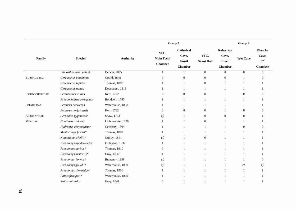
34
Group 1 Group 2
Family Species Authority
VFC,
Main Fossil
Chamber
Cathedral
Cave,
Fossil
Chamber
VFC,
Grant Hall
Robertson
Cave,
Inner
Chamber
Wet Cave
Blanche
Cave,
3rd
Chamber
‘Simosthenurus’ pales‡ De Vis, 1895 1 1 0 0 0 0
BURRAMYIDAE Cercartetus concinnus Gould, 1845 0 0 0 0 1 0
Cercartetus lepidus Thomas, 1888 1 1 0 1 1 1
Cercartetus nanus Desmarest, 1818 1 1 1 1 1 1
PSEUDOCHEIRIDAE Petauroides volans Kerr, 1792 0 0 0 1 0 0
Pseudocheirus peregrinus Boddaert, 1785 1 1 1 1 1 1
PETAURIDAE Petaurus breviceps Waterhouse, 1838 1 1 1 1 1 1
Petaurus norfolcensis Kerr, 1792 0 0 0 1 0 0
ACROBATIDAE Acrobates pygmaeus* Shaw, 1793 cf. 1 0 0 0 1
MURIDAE Conilurus albipes† Lichtenstein, 1829 1 1 0 1 1 1
Hydromys chrysogaster Geoffroy, 1804 1 1 1 1 0 0
Mastacomys fuscus* Thomas, 1882 1 1 1 1 1 1
Notomys mitchellii* Ogilby, 1841 cf. 1 0 1 1 1
Pseudomys apodemoides Finlayson, 1932 1 1 1 1 1 1
Pseudomys auritus† Thomas, 1910 0 1 1 1 1 1
Pseudomys australis* Gray, 1832 1 1 1 1 1 1
Pseudomys fumeus* Brazenor, 1936 cf. 1 1 1 1 0
Pseudomys gouldii† Waterhouse, 1839 cf. 1 1 1 cf. cf.
Pseudomys shortridgei Thomas, 1906 1 1 1 1 1 1
Rattus fuscipes * Waterhouse, 1839 1 1 1 1 1 1
Rattus lutreolus Gray, 1841 0 1 1 1 1 1
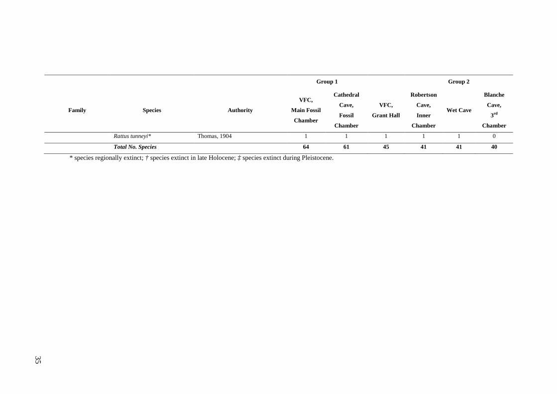
35
Group 1 Group 2
Family Species Authority
VFC,
Main Fossil
Chamber
Cathedral
Cave,
Fossil
Chamber
VFC,
Grant Hall
Robertson
Cave,
Inner
Chamber
Wet Cave
Blanche
Cave,
3rd
Chamber
Rattus tunneyi* Thomas, 1904 1 1 1 1 1 0
Total No. Species 64 61 45 41 41 40
* species regionally extinct; † species extinct in late Holocene; ‡ species extinct during Pleistocene.
36
Climate
An advantage of the Naracoorte Caves for palaeontological study is that they contain
abundant speleothem material which can provide information about local climate
conditions using carbon and oxygen stable isotopes. These can be linked to a high
resolution chronology (U-series dating) and related to regional and global climatic data
(Ayliffe et al., 1998). Speleothems are common secondary calcium carbonate
structures of limestone caves and include stalagmites, stalactites, flowstones and
calcite straws. They form from the precipitation of calcium carbonate from seepage
water that has flowed through the overlying limestone and surface soil horizons into
the cave. Growth and formation of speleothems is controlled by the interaction of a
range of factors including regional temperatures, the amount of water infiltrating from
the surface and the partial pressure of Ca and CO2 in seepage water (Ayliffe et al.,
1998).
It was originally assumed that speleothem growth coincided with interglacial periods
in the past due to higher rainfall when compared with more arid, glacial times (Ayliffe
and Veeh, 1988). However, this was not supported by analysis of a number of
speleothems of differing age from a range of cave sites within the NCWHA (Ayliffe et
al., 1998). In contrast to expectations, speleothem growth coincided with stadial and
cool interstadials (periods of lesser glacial and interglacial extremes) of the Middle to
Late Pleistocene (Ayliffe et al., 1998; Demarshelier et al., 2000; Bestland and Rennie,
2006; Fig. 2.3).
Ayliffe et al. (1998) hypothesised that the lack of speleothem growth in the Naracoorte
Caves over the penultimate interglacial, Marine Isotope Stage (MIS) 5e, reflected
conditions of high evaporation and reduced effective moisture availability as a result of
elevated temperatures. Conversely, temperature declines during glacials and cool
interstadials may have ‘depressed’ evapotranspiration, increasing effective moisture
availability and infiltration through the surface soil horizons and limestone bedrock.
Further, speleothem growth appears to have coincided with average ocean
temperatures at least 3°C lower than present (Ayliffe et al., 1998). This is supported by
pollen deposits in western Tasmania which indicate temperature reductions of greater
than 3.5°C when compared with modern times (Colhoun, 2000), coincident with
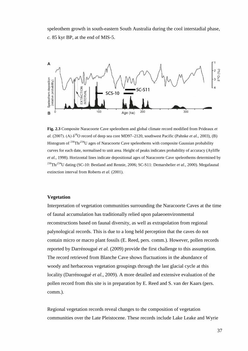
37
speleothem growth in south-eastern South Australia during the cool interstadial phase,
c. 85 kyr BP, at the end of MIS-5.
Fig. 2.3 Composite Naracoorte Cave speleothem and global climate record modified from Prideaux et
al. (2007). (A) δ18O record of deep sea core MD97–2120, southwest Pacific (Pahnke et al., 2003), (B)
Histogram of 230Th/234U ages of Naracoorte Cave speleothems with composite Gaussian probability
curves for each date, normalised to unit area. Height of peaks indicates probability of accuracy (Ayliffe
et al., 1998). Horizontal lines indicate depositional ages of Naracoorte Cave speleothems determined by 230Th/234U dating (SC-10: Bestland and Rennie, 2006; SC-S11: Demarshelier et al., 2000). Megafaunal
extinction interval from Roberts et al. (2001).
Vegetation
Interpretation of vegetation communities surrounding the Naracoorte Caves at the time
of faunal accumulation has traditionally relied upon palaeoenvironmental
reconstructions based on faunal diversity, as well as extrapolation from regional
palynological records. This is due to a long held perception that the caves do not
contain micro or macro plant fossils (E. Reed, pers. comm.). However, pollen records
reported by Darrénougué et al. (2009) provide the first challenge to this assumption.
The record retrieved from Blanche Cave shows fluctuations in the abundance of
woody and herbaceous vegetation groupings through the last glacial cycle at this
locality (Darrénougué et al., 2009). A more detailed and extensive evaluation of the
pollen record from this site is in preparation by E. Reed and S. van der Kaars (pers.
comm.).
Regional vegetation records reveal changes to the composition of vegetation
communities over the Late Pleistocene. These records include Lake Leake and Wyrie
38
Swamp near Millicent in South Australia (Dodson, 1975, 1977) and Lakes Wangoom
(Harle et al., 2002), Bolac and Turangmoroke (Cook, 2009) in south-western Victoria.
Palynological records from marine core E55-6, collected offshore from the southern tip
of south-eastern South Australia, shows that during the cool phase of MIS-2, heath and
grass communities characterised the region (Harle, 1997). In contrast, the records from
Wyrie Swamp and Lake Leake indicate that a mosaic of vegetation types was
maintained on the landscape through the last glacial cycle. This mosaic was
characterised by Eucalyptus woodland with heath understorey and more open
woodlands and grasslands dominated by Asteraceae and Poaceae (Dodson, 1975,
1977).
From the start of the Holocene, regional records document the appearance of more
seasonally adapted species in the vegetation communities (Dodson, 1975; Cook, 2009).
The influence of seasonal water availability across the landscape was a feature
recognised in early historical records from the region (Croft, 2003). As a result of this
seasonality and the variation in landscape features, the pre-European South East
vegetation comprised a “complex mosaic of plant communities” (Croft, 2003, p. 43),
reflecting the early Holocene pollen records from the lower South East and Blanche
Cave (Dodson, 1975, 1977; Darrénougué et al., 2009). The composition of these
communities has been extensively interpreted and described elsewhere from historical
records (Croft, 2003).
The present composition and distribution of vegetation within the Naracoorte Coastal
Plains bioregion reflects the extensive modification and clearance that has occurred in
historical times. Land uses including irrigated agriculture and pasture, forestry and the
expansion of human settlement have reduced native vegetation in the region to only
13% of original coverage (Foulkes and Heard, 2003). Within the NCWHA, very little
remnant vegetation remains, reflecting the impact of historical clearance and the
introduction of non-indigenous native plants and introduced species, including herbs,
annual grasses, broadleaved trees and palms (South East Region National Parks and
Wildlife South Australia (SENPWSA), 2001).
39
Palaeoecology of the NCWHA Against the backdrop of research into the geological setting, diversity and
palaeoenvironmental context of the Naracoorte Caves has been research into the
palaeoecology of the assemblages themselves. Palaeoecological analyses of the fossil
assemblages have focussed on two general aims: (1) to reconstruct past environmental
and climatic conditions from fossil faunas to understand the timing and nature of local
and regional climate change (e.g., McDowell, 2001; Laslett, 2006), and/or (2) to
understand how past climate change affected local faunas (e.g., Moriarty et al., 2000).
Palaeoenvironmental reconstructions Palaeoenvironmental reconstructions are a common technique in palaeoecological
analyses and use a wide range of natural archives including pollen, diatoms, ostracods
and vertebrate faunas to interpret the past environmental and climatic conditions of
different localities. Reconstructions are typically based on the known phenotypic (e.g.,
body size, locomotion, taxonomy) and adaptive (e.g., geographic distribution, habitat
and diet) responses that define the contemporary environmental tolerance ranges of a
species or assemblage (Lundelius, 1964; Andrews and Lord, 1979; Reed, 1998).
Variation in the composition of a fossil assemblage is then assumed to indicate when
and how environmental and/or climatic conditions have changed through time. This is
based on the concept of ‘ecological replacement’ where faunal succession reflects
environmental change (Brenchly and Harper, 1998).
Increasingly, palaeoenvironmental reconstructions have adopted a bioclimatic
modelling approach. Similar to those used in the projection of species distributions
under future climate change scenarios, these models have been developed to
reconstruct past climates using the modern distributions of mammal faunas (e.g.,
Hernández Fernández and Peláez-Campomanes, 2005). However, as recognised by
Shabel et al. (2004), climatic tolerance limits are only one part of an organisms niche;
other factors such as food and habitat availability and interspecific interactions also
control a species geographic distribution and, hence, tolerance limits.
The earliest temporal analyses of fossil faunas of the NCWHA involved
palaeoenvironmental reconstructions based on the small vertebrate remains from Main
Fossil Chamber, VFC. In these reconstructions, the modern distribution and habitat
40
preferences of extant taxa identified in the deposit were used to infer the dominant
vegetation types surrounding the cave at the time of accumulation (Smith, 1971; 1972;
Wells et al., 1984). Later, more sophisticated palaeoenvironmental reconstructions
were conducted using the Late Quaternary aged fossil faunas of Wet, Robertson and
Blanche Cave (McDowell, 2001; Laslett, 2006). In these studies, ecological
characteristics such as habitat preferences, diet, activity and body size were weighted
by the relative abundance of species within each excavation layer to reconstruct Late
Quaternary climate and habitats around the caves, as well as to examine change in
these conditions through the last glacial cycle. In defining the broad ecological niches
of the faunas, McDowell (2001) and Laslett (2006) also considered the functional
diversity of the palaeocommunities.
Smith (1972) suggested that the local vegetation at the time of accumulation of the
assemblage from Main Fossil Chamber, VFC was dry sclerophyllous forest; however,
later reconstructions based on the faunas of other sites have been more specific and
consistently found that a “mosaic” of vegetation types was likely present at various
times throughout the Pleistocene (e.g., McDowell, 2001; Laslett, 2006; Fraser and
Wells, 2008), consistent with the immediately pre-European vegetation communities
of the region as described by Croft (2003). Descriptions of this mosaic have typically
included grasslands and woodlands. Swamps and forests appear to have been persistent
habitat types, but are not as well-represented due to either their rarity in the
palaeoenvironment (e.g., covered smaller areas when compared with grasslands and
woodlands) or poor representation by associated faunas as a result of biases in the
fossil record.
Climate change is presumed to have driven variation in the relative proportion of these
vegetation types through the Pleistocene (Laslett, 2006). For example, the assemblages
from Wet, Robertson and Blanche caves revealed a relatively higher percentage of
grassland-inhabiting faunas in the sand-rich layers associated with MIS-2 (last glacial)
when compared with the younger, organic-rich Holocene aged sediments which
contained a higher percentage of woodland species (McDowell, 2001; Laslett, 2006).
41
Assumptions and inference in palaeoenvironmental reconstructions
While palaeoenvironmental reconstructions are used extensively in palaeoecological
studies, they are also criticised for their reliance on a number of assumptions (e.g.,
Belyea, 2007) and on higher-order extrapolations that may not be accurate (Caran,
1998). Examples of the former include the following assumptions: (a) the
environmental and climatic tolerances of species have not changed over time, (b) the
present-day distribution and ecological preferences (ecological niches) of a species
represent the full limits for that species and (c) present-day habitat types existed in the
past. An example of a higher-order extrapolation, as described by Caran (1998) may
include inferring reduced effective moisture at a given locality based on the last
appearance of a wetland inhabiting species (e.g., lemmings) through the following
sequence of inference: last appearance of remains of lemmings in a fossil sequence =
local extirpation of lemmings = loss of lemming habitat (wetlands) = reduced stream
flow = increased aridity (reduced effective moisture). Clearly, a range of alternative
explanations may account for the absence of lemming remains in a fossil assemblage
from a particular stratigraphic level and need to be considered as alternative
explanations. These include taphonomic or sampling bias, post-depositional loss of
bone bearing sediments, community-level processes such as competition, as well as
factors other than aridity that may reduce the extent of wetland habitats such as
increased rates of water flow and storm events.
Niche preservation through time
It is generally assumed that ecological niches function at the generic level in mammals
and are also conserved at this taxonomic level over time (Hadly et al., 2009).
However, the generality of this assumption has been challenged (e.g., DeSantis et al.,
2009) and may not be valid for all species. For example, using a comparative based
analysis of the pre-European and contemporary small mammal diet of sooty owls (Tyto
tenebricosa tenebricosa), Bilney et al. (2010) demonstrated that the ecological niches
of small mammals in south-eastern Australian forests have been severely
underestimated; niche contraction and denial as a result of restricted distribution and
abundance suggests that the difference between a species’ fundamental and realised
niche is significant (Bilney et al., 2010).
42
Geographic range contraction as a result of historic and contemporary landscape
change is also likely to result in under- or misrepresentation of the climatic range of
many species. An example stemming from the Naracoorte Caves is the Pleistocene
occurrence of Plains Mouse (Pseudomys australis), showing that the species was
formerly present within the vicinity of the caves. However, the species is today
restricted to cracking clays in central Australia and is considered an arid-land species
(Van Dyck and Strahan, 2008). The extent to which the presence of P. australis at
Naracoorte represents more arid climatic conditions in the past, the presence of
cracking clays (or similar substrate), or niche contraction is unknown. It is also
possible that the specimens identified as P. australis represent a cryptic, new species as
suggested for fossil specimens from a fossil locality on Yorke Peninsula (McDowell et
al., 2012), limiting the usefulness of reconstructions based on the observed ecology of
the species today.
There are also problems associated with the definition of the ecological traits of
different species, especially generalist taxa that may use a wide range of habitat types
or dietary items. For example, in the palaeoenvironmental reconstructions based on the
assemblages from Wet and Robertson caves, individual species were, in some cases,
allocated to more than one habitat category (McDowell, 2001). For example, Rattus
fuscipes was counted as a forest, scrub and woodland species. In addition, where the
ecological characteristics of a species were unknown (e.g., for extinct taxa) or where
specimens were identified to genus or family level only, the data were not adjusted to
account for the absence of these taxa in the cumulative per cent data. The effect of
these methods was that the total abundance of faunas in any layer of the assemblage
was either greater than or less than 100%. These challenges make it difficult to assess
the overall robustness of the palaeoenvironmental reconstructions and functional
diversity of Late Pleistocene Naracoorte based on the fossil faunas of Wet and
Robertson Caves.
As a result of these challenges it is generally accepted that reconstructions based on
whole assemblages provide a more accurate reflection of palaeoenvironmental
conditions than those based on a single species (Lowe and Walker, 1997). Further,
Lundelius (1964) argued that multi-taxon based interpretations are required to reduce
the effect of species’ evolutionary adaptation over time. Despite these
43
recommendations, divergence in the abundance trends of taxa that are considered to
have similar ecological niches observed in Naracoorte fossil records shows that
species’ responses to climatic change may not necessary reflect (a) linear relationships
between niches and climate change responses, nor (b) that species with overlapping
niches today had so in the past (Macken et al., 2012). As a consequence,
palaeoecological techniques that focus on functional diversity should attempt, where
possible, to measure functional traits from the fossils rather than through inference
based on modern niches. Functional traits are not considered in this thesis where
attention is given to measures of diversity (e.g., species richness, relative abundance)
but could include body size and diet. Palaeoecological techniques that may be used to
study diet from fossil specimens include microwear (e.g., Rivals and Deniaux, 2003)
and stable carbon isotopes (DeSantis et al., 2009).
No-analogue assemblages
An outcome of historic contraction in the geographic, and hence climatic and habitat
ranges of many species, is the occurrence of no-analogue assemblages in Quaternary
fossil deposits. ‘No-analogue assemblage’ is used to describe the co-occurrence of
species in fossil deposits that have allopatric distributions today (Lundelius, 1989). No-
analogue assemblages are common in Pleistocene fossil deposits and typically result in
greater estimates of species diversity in Pleistocene communities than those of the
Holocene and present. This is commonly attributed to more equable climates with less
seasonal extremes and greater habitat diversity during the Pleistocene when compared
with today (e.g., Graham, 1985; Lundelius, 1989; Carrasco et al., 2009; Ceballos et al.,
2010). Evidence that is commonly used to support this assumption is the severity of
global climate change at the Pleistocene–Holocene transition (Graham, 1985);
however, this perspective contrasts with the more general view of Swetnam et al.
(1999) who suggested that no-analogue assemblages represent changed physical and
biological recording processes and their interaction with the environment through time.
In order to avoid the issues associated with no-analogous assemblages, Carrasco et al.
(2009) assessed change through time in North America faunas from 30 million to 500
years ago. In reconstructing the pre-European baseline of biodiversity, they were able
to maintain the same sampling and analytical techniques for all temporal periods,
rather than comparing the fossil samples against the highly modified faunal diversity
44
of modern times. McDowell (2001) used a similar approach in his analysis of the Late
Quaternary aged deposits from Wet Cave where he aimed to reconstruct the
immediately pre-European mammal community of the Naracoorte region. The purpose
was to provide a pre-impact baseline from which to compare Pleistocene
palaeocommunity diversity. Unfortunately, the immediately pre-European fossil
assemblage from Wet Cave contained older, re-worked Pleistocene aged fossil
material, limiting its usefulness for such a comparison (McDowell, 2001).
Climate change effects on local faunas In comparison to these examples of palaeoenvironmental reconstructions, Moriarty et
al. (2000) presented the first appraisal of faunal responses to climate change from the
Naracoorte Caves. Their study represented an important shift in the focus or type of
research question being addressed through analysis of the Naracoorte Caves fossil
faunas; that is, rather than reconstructing conditions based on the fossil assemblages,
Moriarty et al. (2000) were the first to explicitly consider what effect climate change
had on the fauna themselves.
As argued by Moriarty et al. (2000), changes in faunal diversity are expected to have
occurred during periods of “climate stress” (p. 140). However, in their assessment of
the composition of six Middle Pleistocene aged assemblages of the NCWHA, Moriarty
et al. (2000) concluded that there had been “little apparent change in faunal diversity
over a period of 300 kyr BP in the Middle Pleistocene, a period spanning at least three
glacial-interglacial cycles” (p. 141).
Subsequent analyses of faunal responses to climate change from assemblages of the
Naracoorte Caves have shown that this model of limited faunal change is simplistic
and, in light of more rigorous sampling in other deposits, unsupported. For example, in
their study of the mammal assemblage of Main Fossil Chamber, Cathedral Cave (one
of the sites examined by Moriarty et al., 2000), Prideaux et al. (2007) found evidence
for change in the relative abundance of individual species between sedimentary units
associated with wetter and drier climatic phases of the Middle Pleistocene (Fig. 2.4a).
The site also showed that there was a local decline in the density of larger mammals,
including megafauna, as the climate became more arid over the transition from MIS-9
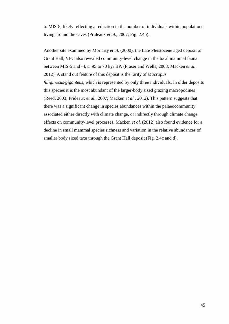
45
to MIS-8, likely reflecting a reduction in the number of individuals within populations
living around the caves (Prideaux et al., 2007; Fig. 2.4b).
Another site examined by Moriarty et al. (2000), the Late Pleistocene aged deposit of
Grant Hall, VFC also revealed community-level change in the local mammal fauna
between MIS-5 and -4, c. 95 to 70 kyr BP. (Fraser and Wells, 2008; Macken et al.,
2012). A stand out feature of this deposit is the rarity of Macropus
fuliginosus/giganteus, which is represented by only three individuals. In older deposits
this species it is the most abundant of the larger-body sized grazing macropodines
(Reed, 2003; Prideaux et al., 2007; Macken et al., 2012). This pattern suggests that
there was a significant change in species abundances within the palaeocommunity
associated either directly with climate change, or indirectly through climate change
effects on community-level processes. Macken et al. (2012) also found evidence for a
decline in small mammal species richness and variation in the relative abundances of
smaller body sized taxa through the Grant Hall deposit (Fig. 2.4c and d).
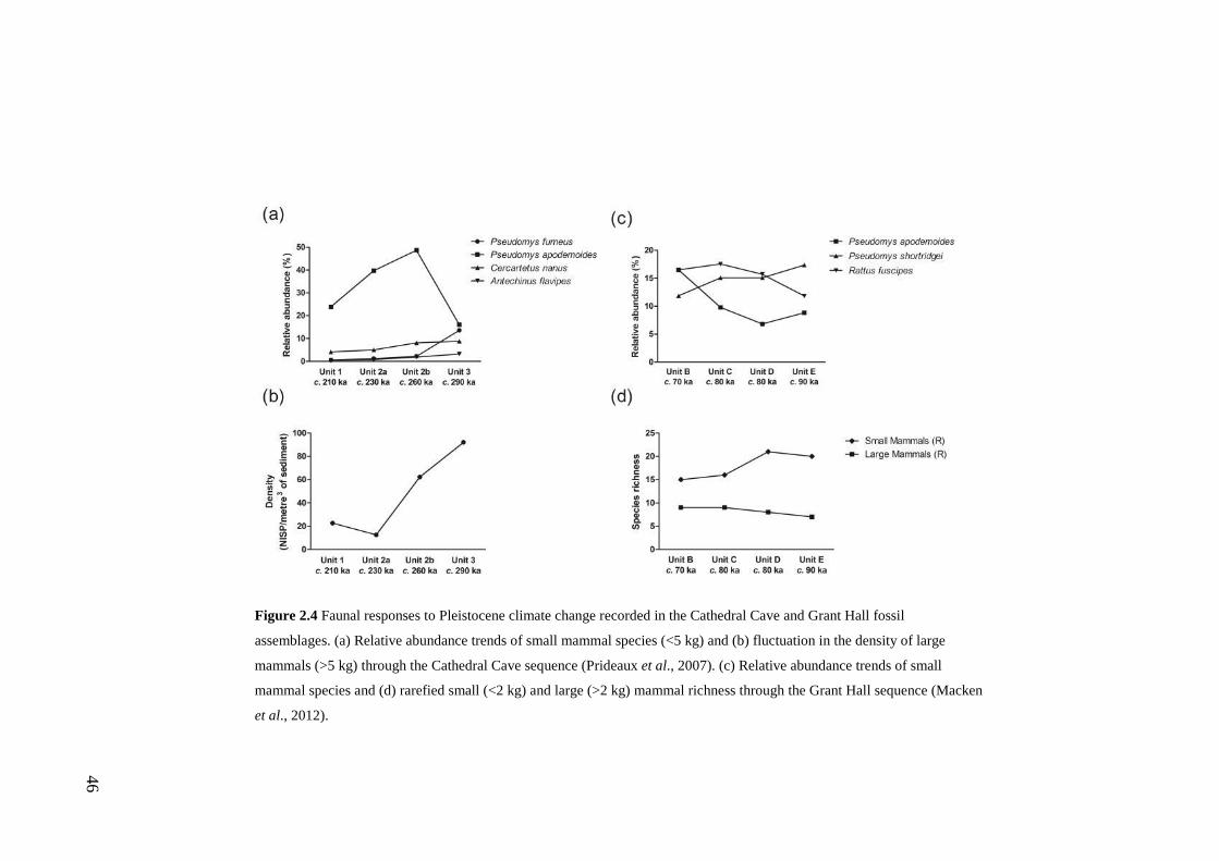
46
Figure 2.4 Faunal responses to Pleistocene climate change recorded in the Cathedral Cave and Grant Hall fossil
assemblages. (a) Relative abundance trends of small mammal species (<5 kg) and (b) fluctuation in the density of large
mammals (>5 kg) through the Cathedral Cave sequence (Prideaux et al., 2007). (c) Relative abundance trends of small
mammal species and (d) rarefied small (<2 kg) and large (>2 kg) mammal richness through the Grant Hall sequence (Macken
et al., 2012).
47
Species-area effects on the detection of faunal responses to climate change
The contrast between Moriarty et al.’s (2000) observation of limited faunal change
against the evidence for variation in species richness, density and abundances from
other studies raises questions about how and why such different conclusions may be
drawn from the same fossil sites. While the reasons are more obvious when
comparing the sampling designs of these studies, different observations from the
same sites suggests that sampling and analytical methods exert a strong influence on
observed ecological patterns and can influence the inferred significance of those
patterns (Rahel, 1990; DiMichele et al., 2004).
The particular sampling concerns of the study by Moriarty et al. (2000) relate to
time-averaging (temporal scale) and inadequate and highly variable sample sizes
between samples (sampling effects). These are commonly cited issues associated
with the analysis of palaeoecological assemblages, including those designed as
palaeoenvironmental reconstructions and are related to the mathematical
relationship between sampling area and species richness (the species-area curve;
Lomolino, 2000). That is, the greater the geographic area sampled by a deposit (and
hence range of environments and climatic zones) the higher its species diversity
(e.g., Barnosky et al., 2005).
Time-averaging and sampling-effort demonstrate a similar relationship with species
richness as geographic sampling area and are related to sampling issues associated
with the fidelity of a fossil assemblage to the living palaeocommunity from which it
was sampled. This is an important consideration in palaeoecology as it affects the
accuracy of data derived from natural archives to the true ecological patterns
exhibited in the past. Sampling biases associated with this relationship typically
concern taphonomic factors (e.g., accumulation mode, agent and depositional
history) in addition to temporal and spatial scale, and sampling biases. As these
issues have been extensively examined for a wide range of sites and types of
palaeoecological archives (e.g., Kidwell and Flessa, 1996, Terry 2010a; b),
particular attention is given here to the influence of sampling effects on observed
patterns, not necessarily the relationship between the observed patterns and the
sampled palaeocommunity.

48
Time-averaging
Time averaging is defined by Hadly and Barnosky (2009) as the number of years
over which a community sample accumulated, with examples of time-averaging
scales for different palaeoecological settings provided in Roy et al. (1996). Greater
time averaging, either through post-depositional or analytical mixing of faunas of
different ages, or through slow accumulation and burial, is expected to inflate
species richness by (a) increasing the likelihood of sampling rare fauna and (b)
sampling successive faunal communities from a single locality. These processes can
result in the consolidation of fauna from different environmental ‘regimes’ into one
assemblage (Graham, 1985). The effect of time-averaging across multiple climatic
phases has been termed ‘climate-mixing’ by Hopely and Maslin (2010) and results
in a weakened signal of climate effects on faunas (Stenseth and Mysterus, 2005).
From a more general perspective, it also means that the term ‘palaeocommunity’ is
not comparable to ‘community’ as used in neontolgoical studies. ‘Community’ is
used to describe an interacting assemblage of species at a particular time and place.
The term ‘palaeocommunity’ is used throughout the thesis, following the definition
of Bennington and Bambach (1996; Table 2.3) and with acknowledgement of its
limitations given time-averaging within fossil assemblages.
In the analysis by Moriarty et al. (2000), faunal change was assessed through a
comparison of the richness and composition of mammal faunas among six
assemblages of Middle Pleistocene age (Table 2.2). However, there were no
stratigraphic and chronological controls assigned to the faunas within those sites
and as acknowledged by Moriarty et al. (2000), this sampling effect introduced
gross time-averaging to the fossil data presented.
As shown in the analysis of the Cathedral Cave and Grant Hall deposits by Prideaux
et al. (2007) and Macken et al. (2012), time-averaging by Moriarty et al. (2000)
mixed faunas of at least two climatic phases in both sites (MIS-9 to MIS-8 and
MIS-5a to MIS-4, respectively). Although the poor chronological resolution and
few data for Main Fossil Chamber of VFC makes it difficult to assess the extent of
time-averaging of the faunas in this deposit when it is considered as a whole, the
presence of sedimentary layers and structures clearly reflects separate stages of
deposition (Wells et al., 1984; Reed, 2003). As a consequence, any differences in
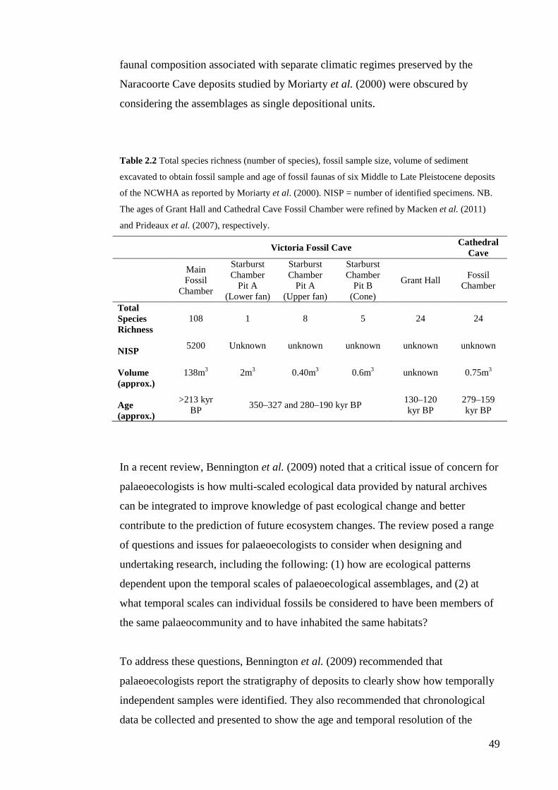
49
faunal composition associated with separate climatic regimes preserved by the
Naracoorte Cave deposits studied by Moriarty et al. (2000) were obscured by
considering the assemblages as single depositional units.
Table 2.2 Total species richness (number of species), fossil sample size, volume of sediment
excavated to obtain fossil sample and age of fossil faunas of six Middle to Late Pleistocene deposits
of the NCWHA as reported by Moriarty et al. (2000). NISP = number of identified specimens. NB.
The ages of Grant Hall and Cathedral Cave Fossil Chamber were refined by Macken et al. (2011)
and Prideaux et al. (2007), respectively.
Victoria Fossil Cave Cathedral Cave
Main Fossil
Chamber
Starburst Chamber
Pit A (Lower fan)
Starburst Chamber
Pit A (Upper fan)
Starburst Chamber
Pit B (Cone)
Grant Hall Fossil Chamber
Total Species Richness
108 1 8 5 24 24
NISP 5200 Unknown unknown unknown unknown unknown
Volume (approx.)
138m3 2m3 0.40m3 0.6m3 unknown 0.75m3
Age (approx.)
>213 kyr BP 350–327 and 280–190 kyr BP 130–120
kyr BP 279–159 kyr BP
In a recent review, Bennington et al. (2009) noted that a critical issue of concern for
palaeoecologists is how multi-scaled ecological data provided by natural archives
can be integrated to improve knowledge of past ecological change and better
contribute to the prediction of future ecosystem changes. The review posed a range
of questions and issues for palaeoecologists to consider when designing and
undertaking research, including the following: (1) how are ecological patterns
dependent upon the temporal scales of palaeoecological assemblages, and (2) at
what temporal scales can individual fossils be considered to have been members of
the same palaeocommunity and to have inhabited the same habitats?
To address these questions, Bennington et al. (2009) recommended that
palaeoecologists report the stratigraphy of deposits to clearly show how temporally
independent samples were identified. They also recommended that chronological
data be collected and presented to show the age and temporal resolution of the
50
individual samples, the position of potential gaps in the record and the overall
temporal range of the sequence.
As noted earlier, cave deposits are considered to be less than ideal for
palaeoecological studies. This is because of the general difficulties associated with
dating depositional sequences and the long-time averaging of these deposits when
compared with other palaeoecological sites such as lake beds or marine sediments
(Lowe and Walker, 1997; Forbes et al., 2007). Cave deposits and other vertebrate
fossil assemblages also generally provide unevenly sampled faunas through time,
such that time-averaging varies between units or layers within an assemblage, as
well as between sites (Roy et al., 1996). Despite these limitations, the majority of
research into the fossil deposits of the NCWHA has involved extensive
sedimentary, stratigraphic and chronological analyses. While the scale of time-
averaging cannot be standardised across or within a deposit, the use of these
techniques fulfils many of the recommendations by Bennington et al. (2009) and
have been critical in enabling more robust analysis of faunal change with time (e.g.,
Forbes and Bestland, 2007; Prideaux et al., 2007; Darrénougué et al., 2009; Macken
et al., 2011).
Sample-size
Differences in sampling effort also strongly influenced the comparative data
presented by Moriarty et al. (2000), challenging both the technique used to assess
faunal change with time and the robustness of their conclusions based on the
available data. Of particular concern are the different species richness values
presented by Moriarty et al. (2000) which ranged from 108 species for Main Fossil
Chamber, VFC, to only one for the lower fan of Spring Chamber, VFC (Table 2.2).
The second highest species richness value was 24, reported for Fossil Chamber,
Cathedral Cave and Grant Hall, VFC (Moriarty et al., 2000). The magnitude of
difference between these species richness values questions the validity of their
conclusion that faunal composition did not differ significantly between these
deposits, for how can composition be judged to be the same when comparing 108
species against 24 or one?
51
The difference in species richness values of these assemblages clearly reflects
variation in sampling effort at the time of the original study (Table 2.2). Moriarty et
al. (2000) acknowledged this limitation, stating that the small sample sizes from
each site except Main Fossil Chamber, VFC “preclude any statistical analysis of
faunas” (p. 140). Although sample size was only reported for one assemblage, the
difference in excavation volume for each deposit suggests that the fossil samples
were of vastly different sizes (Table 2.2). A similar issue was identified in the
analysis of Graham et al. (1996), where sampling variation was suggested to have
biased the raw presence/absence data used to assess change in the geographic
distribution of North American vertebrates over the Quaternary (Alroy, 1999).
Analytical standardisation techniques are commonly applied to fossil occurrence
data to account for variation in sample size between deposits and depositional units
within single sites. Techniques include analytic rarefaction, where the richness of
different depositional units is estimated based on a standard sample size, usually the
smallest sample size of the units within a deposit (e.g., Prideaux et al., 2007).
Hammer and Harper (2006) provide a brief discussion of other mathematical
richness estimation techniques including first and second order jack-knife and
bootstrapping.
Bootstrapping has been used on small mammal assemblages for comparing species
richness through time and between different types of samples (e.g., Blois et al.,
2010; Terry, 2010a; b). The technique involves re-sampling with replacement from
an assemblage until a pre-determined number of sub-samples have been generated,
often 1000 (Chernick, 2008). Using bootstrapping, confidence limits on statistics
(e.g., species richness) measured from an assemblage may be generated (e.g., Blois
et al., 2010). Bootstrapping may re-sample an assemblage to either the original
sample size or a predetermined sample size, often corresponding to the smallest
sample size measured from each layer within a stratigraphic sequence.
Sample size can also influence the representativeness of a fossil sample in relation
to the full range of species preserved in a depositional setting. The
representativeness of a fossil sample is also commonly assessed using analytic
rarefaction. In this procedure, it is assumed that as the slope of the cumulative
52
species curve approaches zero, the probability of additional specimens representing
new species declines to a point where further excavation effort is unlikely to
dramatically increase species richness. For example, Laslett (2006) reported
specimen counts ranging from a minimum of 58 to a maximum of 1777 from the
five units analysed from Blanche Cave. A rarefaction curve constructed by Laslett
(2006) for the whole deposit suggested that a minimum sample of 1200 specimens
adequately sampled the true richness of species preserved in the deposit. When this
figure was applied to the individual units, only two were expected to have adequate
specimens to accurately represent species richness (Laslett, 2006).
Defining natural variation and resilience in palaeoecological
systems
Resilience of Naracoorte mammal faunas to past climate change As shown in the faunal analyses of Prideaux et al. (2007) and Macken et al. (2012),
the Moriarty et al. (2000) model of ‘no faunal change’ for the Naracoorte Cave
faunas was strongly influenced by sampling effects. However, based on the lack of
evidence for local faunal extinctions, Prideaux et al. (2007) argued that the Middle
Pleistocene mammal faunas of south-eastern South Australia were resilient to
Pleistocene climate change. While this conclusion has implications for
understanding the drivers of megafaunal extinction in Australia, it is also significant
from a broader ecological perspective.
Of particular interest is the observation that the abundances and/or presence/absence
of individual mammal species did in fact fluctuate in response to Pleistocene
climate change, but that this did not result in their extinction. This suggests that,
despite climatic and environmental disturbances, faunal changes occurred within
thresholds relating to the survival, reproduction, interspecific interactions and
dispersal of populations.
As defined by Groffman et al. (2006), an ecological threshold represents either a
point of abrupt change in an ecosystem “quality, property or phenomenon”, or
where small environmental changes cumulatively lead to large ecosystem responses
(p. 1). In the case of the Naracoorte mammal faunas, the ecosystem property
considered by Prideaux et al. (2007) was individual species persistence and/or
53
survival through the Pleistocene. However, despite the long-term survival of
individual species evident in the Naracoorte Cave assemblages, there is also
evidence for palaeocommunity change. Of note is the decline in richness of small
mammals in the palaeocommunity over the accumulation of Grant Hall and the
lower overall richness of small mammals in this deposit when compared with both
older and younger assemblages (Macken et al., 2012; Table 2.1; Fig. 2.4c). These
patterns suggest that the composition of the small mammal palaeocommunity was
not stable throughout the Pleistocene and that the palaeocommunity as a whole may
not have been resilient to climate change.
Natural variation/resilience framework Increasingly, theoretical concepts of natural variation have been identified as a
useful framework for evaluating change in palaeoecological assemblages (Hadly
and Barnosky, 2009). Natural variation is defined as the normal range of
fluctuations and trends in ecosystem attributes, condition and/or processes within an
ecological system across space and time (Landres et al., 1999). Biodiversity
conservation and management strategies increasingly aim to manage for natural
variation in ecosystems given the advantages of this approach when compared with
more traditional management strategies that focus on a single steady-state. These
advantages include greater cost-effectiveness and lack of reliance on a single pre-
impact state that may or may not be well defined or relevant in the context of
modern and future societal, ecological and climatic parameters (Landres et al.,
1999; Swetnam et al., 1999).
Even more significant than these factors in explaining the increased attention on
natural variation in ecological management is the relationship between natural
variation and resilience. Natural variation provides an ecological ‘buffer,’ allowing
ecosystems to undergo turnover and reorganise in response to external pressures,
whilst maintaining ecological functions, structure, ecological connections and
general character or type (Holling and Meffe, 1996; Folke et al., 2004; Walker et
al., 2004).
As noted in the introduction, ‘resilience’ generally describes how much pressure or
change an ecological system can withstand before it shifts to a new, alternative
54
steady-state (Holling, 1996; Walker et al., 2009). This definition contrasts with the
concept of ‘engineering resilience’ which describes how quickly a system recovers
following a disturbance event (Holling, 1996). This latter definition is based on an
assumption that ecosystem equilibrium occurs through the persistence of a single
steady-state; that is, a system returns to its pre-disturbance condition following a
period of change.
While the former definition is generally considered most suitable for describing
resilience in ecological systems, resilience is very difficult to quantify (North and
Stein, 2012). This difficulty arises in part because more complex definitions of
resilience incorporate aspects of both ecological and engineering resilience; that is,
change and reorganisation coupled with maintenance of “essentially the same
ecosystem function, structure, identity and feedbacks” (Walker et al., 2004; p1).
Inherent within any concept of resilience are thresholds which represent the limits
of change that an ecological system can undergo before its fundamental properties
are shifted to a new state or regime. Thus, critical questions that emerge for
quantifying the resilience of a system include: (a) how much change can an
ecological system absorb or experience before ecosystem functions, structure,
identity and feedbacks are no longer maintained? (b) If these properties do change,
how are they judged to be either “essentially the same” (Walker et al., 2004, p.1), or
significantly different, and (c) can a system be considered resilient if only its
identity changes, but function and structure are maintained?
While these questions are generally posed in relation to the management of
contemporary ecosystems, they are relevant to the study of faunal and other
ecological and environmental changes observed in palaeoecological assemblages.
DiMichele et al. (2004) noted there are no clear guidelines from which to assess if
changes observed in palaeoecological assemblages represent significant
palaeocommunity change. In other words, how is significant palaeocommunity
change or reorganisation defined and when do such changes represent a breach of
resilience thresholds?
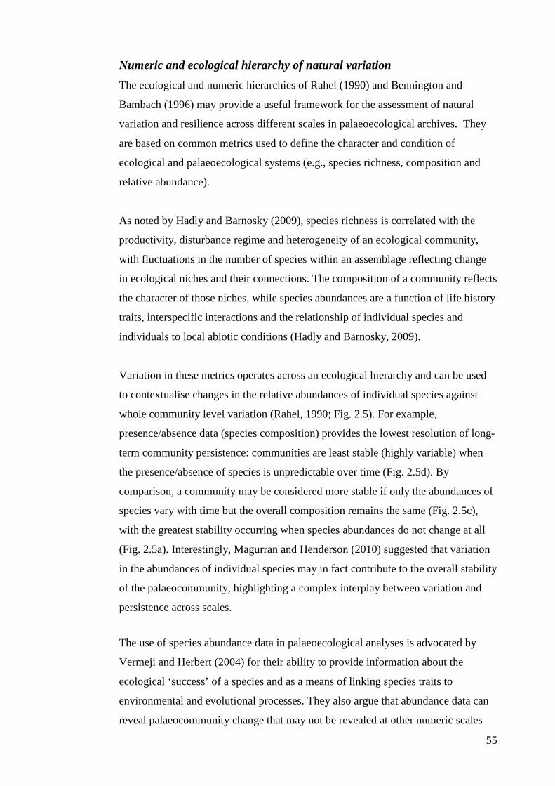
55
Numeric and ecological hierarchy of natural variation The ecological and numeric hierarchies of Rahel (1990) and Bennington and
Bambach (1996) may provide a useful framework for the assessment of natural
variation and resilience across different scales in palaeoecological archives. They
are based on common metrics used to define the character and condition of
ecological and palaeoecological systems (e.g., species richness, composition and
relative abundance).
As noted by Hadly and Barnosky (2009), species richness is correlated with the
productivity, disturbance regime and heterogeneity of an ecological community,
with fluctuations in the number of species within an assemblage reflecting change
in ecological niches and their connections. The composition of a community reflects
the character of those niches, while species abundances are a function of life history
traits, interspecific interactions and the relationship of individual species and
individuals to local abiotic conditions (Hadly and Barnosky, 2009).
Variation in these metrics operates across an ecological hierarchy and can be used
to contextualise changes in the relative abundances of individual species against
whole community level variation (Rahel, 1990; Fig. 2.5). For example,
presence/absence data (species composition) provides the lowest resolution of long-
term community persistence: communities are least stable (highly variable) when
the presence/absence of species is unpredictable over time (Fig. 2.5d). By
comparison, a community may be considered more stable if only the abundances of
species vary with time but the overall composition remains the same (Fig. 2.5c),
with the greatest stability occurring when species abundances do not change at all
(Fig. 2.5a). Interestingly, Magurran and Henderson (2010) suggested that variation
in the abundances of individual species may in fact contribute to the overall stability
of the palaeocommunity, highlighting a complex interplay between variation and
persistence across scales.
The use of species abundance data in palaeoecological analyses is advocated by
Vermeji and Herbert (2004) for their ability to provide information about the
ecological ‘success’ of a species and as a means of linking species traits to
environmental and evolutional processes. They also argue that abundance data can
reveal palaeocommunity change that may not be revealed at other numeric scales
56
(such as composition), as is evident in the fossil assemblages of the NCWHA.
Species level changes in palaeoecological records also indicate those species that
have been most sensitive to past climate change (Dietl and Flessa, 2010).
Figure 2.5 Numeric hierarchy of stability demonstrated in a hypothetical assemblage of five species
(A–E). (a) Species’ abundances are highly stable (no variation). (b) There is variation in species
abundances, but their rank-order stays the same. (c) Variation in species’ abundances leads to
variation in the rank-order of the species. (d) Species’ abundances are so variable that even the
presence/absence of species’ is unpredictable. Modified from Rahel (1990).
57
Based on their review of vertebrate responses to climate change from a range of
fossil localities, Hadly and Barnosky (2009) suggested that changes in the relative
abundances of species are the “early warning signal” of environmental effects on
species (p. 47). However, they also argued that changes in species relative
abundance alone do not constitute significant change from a normal baseline of
variation operating at the species level within a palaeocommunity (Hadly and
Barnosky, 2009). Rather, based on evidence from fossil and modern assemblages,
they suggested that variation in the relative abundances of species is the normal
type of response to climate change and other disturbances across different temporal
scales.
When then, if ever, are changes in species abundances in fossil assemblages
ecologically significant in terms of assessing faunal change through time? The first
step to addressing this question may be to assess the statistical significance of
change in these ecological variables, as according to Bennington and Bambach
(1996), after site-effects are accounted for, if two samples have statistically
different species abundance distributions then they may be assumed to have come
from different palaeocommunity types (Table 2.3). In this context,
palaeocommunity types are separated on the basis of having similar, but not
statistically identical species abundance distributions (Bennington and Bambach,
1996). Within these definitions, it is acknowledged that given the extent of time-
averaging, biasing and information loss through taphonomic processes in fossil
assemblages, a local palaeocommunity is not equivalent to a local community
observed in neontolgoical studies where contemporaneity can be established.
However, the numeric hierarchy of Rahel (1990) and discussions of Hadly and
Barnosky (2009) caution that the relative abundances of species can be highly
variable with time and may not necessary reflect ecologically significant change
between local palaeocommunities. An intermediate level within Rahel’s (1990)
numeric hierarchy is rank-order abundance. A commonly used measure of
abundance ranks is Spearman’s Rho. This metric has been used in the analysis of
fossil assemblages, particularly to assess the fidelity of live-dead assemblages (e.g.,
Kidwell 2001; Terry 2010a; b). It is also used in a wide range of ecological studies
(e.g., Rabonsky et al., 2011) and has been suggested as a useful measure for
58
detecting early signs of change in ecological assemblages (Magurran and
Henderson 2010).
Of particular interest then for the fossil assemblages of the Naracoorte Caves is
whether the relative abundance of species varied sufficiently to lead to a new rank-
order abundance structure. An ecological driver of stability in abundance ranks may
be synchrony of changes in the relative abundance of species within a community in
response to disturbance, reflecting similar responses of individual species to
environmental or climatic changes (Rahel, 1990). However, based on the observed
fluctuations in the relative abundances of species in assemblages of the Naracoorte
Caves (e.g., Macken et al., 2012), synchronous responses are very rare. For
example, while some species demonstrated similar patterns of change in response to
transitions from relatively dry to relatively wet conditions and visa-versa between
the Cathedral Cave and Grant Hall assemblages (Macken et al., 2012), not all
species with similar ecological characteristics (e.g., dietary and habitat preferences)
had the same pattern of response within the two sites. Further, some species
demonstrated different responses to the climate changes between the two sites
(Prideaux et al., 2007; Macken et al., 2012). These divergent patterns in species
abundance are consistent with evidence elsewhere for individualistic species
responses to climate change (Stewart, 2008). They also likely reflect the influence
of other factors on species responses, including a combination of environmental and
climatic thresholds and community and population dynamics associated with
intrinsic responses described by Williams et al. (2011).
Intrinsic responses are those changes associated with non-linear ecological
processes, thresholds and tipping points and are characterised by variable timings
and rates of change among species and localities. Extrinsic ecological changes are
driven by external, abrupt climate changes and are characterised by synchronous
biotic responses within and between localities (Williams et al., 2011). While
extrinsic responses are clearly important in revealing the drivers and general
responses to change operating at large temporal and spatial scales, intrinsic
responses are expected to reveal more about the past resilience of ecosystems and
the range of variation exhibited by different ecosystem components in response to
disturbances operating across spatial and temporal scales.
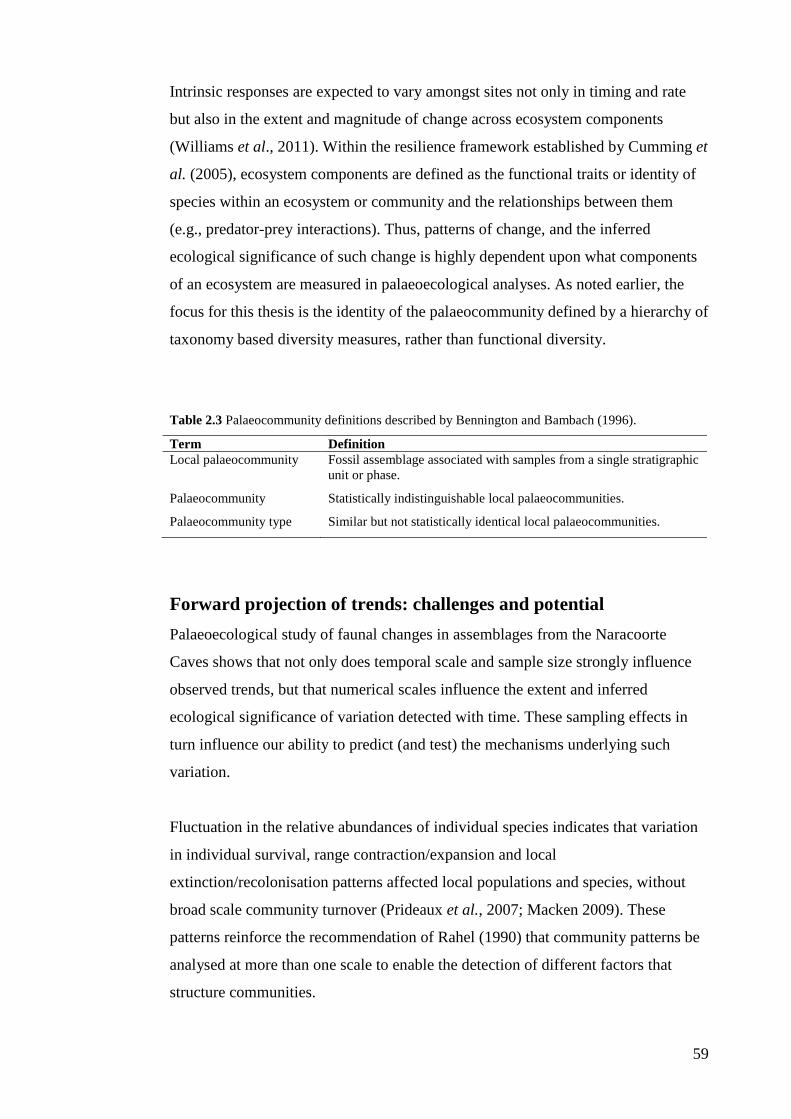
59
Intrinsic responses are expected to vary amongst sites not only in timing and rate
but also in the extent and magnitude of change across ecosystem components
(Williams et al., 2011). Within the resilience framework established by Cumming et
al. (2005), ecosystem components are defined as the functional traits or identity of
species within an ecosystem or community and the relationships between them
(e.g., predator-prey interactions). Thus, patterns of change, and the inferred
ecological significance of such change is highly dependent upon what components
of an ecosystem are measured in palaeoecological analyses. As noted earlier, the
focus for this thesis is the identity of the palaeocommunity defined by a hierarchy of
taxonomy based diversity measures, rather than functional diversity.
Table 2.3 Palaeocommunity definitions described by Bennington and Bambach (1996).
Term Definition Local palaeocommunity Fossil assemblage associated with samples from a single stratigraphic
unit or phase.
Palaeocommunity Statistically indistinguishable local palaeocommunities.
Palaeocommunity type Similar but not statistically identical local palaeocommunities.
Forward projection of trends: challenges and potential Palaeoecological study of faunal changes in assemblages from the Naracoorte
Caves shows that not only does temporal scale and sample size strongly influence
observed trends, but that numerical scales influence the extent and inferred
ecological significance of variation detected with time. These sampling effects in
turn influence our ability to predict (and test) the mechanisms underlying such
variation.
Fluctuation in the relative abundances of individual species indicates that variation
in individual survival, range contraction/expansion and local
extinction/recolonisation patterns affected local populations and species, without
broad scale community turnover (Prideaux et al., 2007; Macken 2009). These
patterns reinforce the recommendation of Rahel (1990) that community patterns be
analysed at more than one scale to enable the detection of different factors that
structure communities.
60
Insights into the range, scale and types of ecological responses to past climate
change gained from fossil assemblages may be used to address the questions
identified at the start of this review. These were (a) how do ecosystems respond in
the short and long-term to disturbance (including climate change), (b) what is the
natural range of variability expressed by an ecosystem at different spatial, temporal
and ecological scales and (c) what are the limits of resilience, or thresholds beyond
which an ecosystem changes state? Biodiversity conservation strategies that
develop the adaptive and resilience capacity of communities and species to future
climate change may be enhanced by knowledge that addresses these questions.
As recognised by Lyman (2006), collaborations between ecology, palaeontology
and conservation biology are imperative for biodiversity conservation in light of the
threats posed by future climate change on species, communities and ecosystems. By
focussing on the data needs of resource managers and using relatively simple, easily
interpreted metrics, palaeontological studies may overcome some of the challenges
associated with the application of past histories to biodiversity conservation today.
However, Swetnam et al. (1999) warn that past trends cannot be directly
extrapolated to present or future conditions. Rather, they argue that long-term
perspectives can guide the development and testing of predictive models and
generate hypotheses that can be tested. Further, they can inform biodiversity
managers about the limits or thresholds inherent in an ecological and environmental
setting, and may provide a context for current landscape conditions. According to
Swetnam et al. (1999), we must “decide if past mechanisms of change and the
dynamical processes involved are desirable for today’s landscapes” (p. 1202). This
requires an acknowledgement of the limitations of ecosystems; we can’t exceed
these without causing system collapse (Swetnam et al., 1999). Patterns of natural
variation in small mammal palaeocommunity composition and structure through the
last glacial cycle provide a unique opportunity to examine and identify these limits
or constraints across time scales far exceeding those available to traditional
ecological studies.
61
3. Chronology and stratigraphy of the Wet Cave vertebrate
fossil deposit, Naracoorte, and relationship to paleoclimatic
conditions of the Last Glacial Cycle in south-eastern
Australia
Citation Macken, A.C., McDowell, M.C., Bartholomeusz, D.H. and Reed, E.H. (2013)
Chronology and stratigraphy of the Wet Cave vertebrate fossil deposit, Naracoorte,
and relationship to paleoclimatic conditions of the Last Glacial Cycle in south-
eastern Australia. Australian Journal of Earth Sciences 60, 271–281.
Contribution of Authors Amy Macken:
• Devised and planned the project.
• Compiled and assessed the data on the Wet Cave stratigraphy and
sediments presented in the paper and identified stratigraphic units for the
deposit based on these data.
• Sourced grant of $1000.00 from the Linnean Society of New South Wales
to support costs associated with additional radiocarbon dating for the site.
• Selected and prepared additional charcoal samples for radiocarbon dating.
• Reviewed the palaeoclimatic literature presented in the manuscript.
• Prepared the manuscript for publication.
Matthew McDowell:
• Provided the original descriptions of the Wet Cave sediments and the
stratigraphic diagram of sedimentary layers in his Masters thesis.
• Provided comments on the manuscript.
62
David Bartholomeusz:
• Led the excavation of the Wet Cave site in 1997 and 1998 and provided
sedimentary descriptions and photographs of the exposed profile in his
field note books.
• Provided comments on the manuscript.
Elizabeth Reed:
• Provided funding for the additional radiocarbon dating.
• Provided comments on the manuscript.
Signed .................................................................................. Date ............................
Amy Macken
School of Biological Sciences, Flinders University
Signed .................................................................................. Date ............................
Matthew McDowell
School of Biological Sciences, Flinders University
Signed .................................................................................. Date ............................
David Bartholomeusz
School of Biological Sciences, Flinders University
Signed .................................................................................. Date ............................
Elizabeth Reed
School of Biological Sciences, Flinders University
63
Abstract The Wet Cave vertebrate fossil deposit of the Naracoorte Caves in south-eastern
South Australia contains a rich and diverse assemblage of small mammal fauna
known to span the Upper Pleistocene–Holocene. Here, we describe five previously
unidentified in situ units (A, B, C, E and F) and one likely reworked unit (D) in the
Wet Cave sedimentary profile, which are correlated with paleoclimatic conditions
associated with the Last Glacial Cycle. Additional radiocarbon dates presented here
provide a finer temporal resolution for the upper sections of the sequence than
previously available and reveal rapid deposition of polished quartz sands laminated
with brown silts during the last glacial maximum (LGM). Change in sediment type
and depositional processes are dated from 16.8–16.4 k cal y BP and are associated
with the onset of deglaciation. The characteristics of the five in situ depositional
units are similar to those identified from the contemporaneous fossil and
sedimentary sequence of Blanche Cave 3rd Chamber, located approximately 400 m
away, reflecting interactions between paleoclimate, sediment mobility and
deposition at this locality. Greater variation is evident between the Wet Cave
sedimentary profile and the inner chamber of Robertson Cave, located
approximately 6 km away and shows that local processes and cave structure exerted
some control on sediment accumulation. Paleoclimatic inferences from the
depositional sequence of Wet Cave are broadly consistent with those inferred from
regional landforms for south-eastern Australia but provide a local signal more
suitable for cross-correlation of the fossil faunas. In particular, the Wet Cave
sequence suggests that local conditions were relatively stable in the lead up to the
LGM despite fluctuation in both local and regional effective precipitation.
Sedimentary units associated with the post LGM deglaciation are characterised by
alternating sand and sandy-silt layers, assumed to reflect the impact of enhanced
seasonality and/or climatic fluctuation leading towards the Holocene.
Keywords cave sediments, Last Glacial Cycle, Naracoorte Caves, paleoclimate,
radiocarbon dating, stratigraphy
64
Introduction The Upper Pleistocene–Holocene sedimentary and fossil sequences of Wet Cave
(5U10, 11) were first studied by McDowell (2001), following excavation of the site
in 1997 and 1998. Re-evaluation of the Wet Cave small mammal fauna (body mass
≤2 kg) and comparison with more recently excavated, contemporaneous deposits of
the Naracoorte Caves World Heritage Area (NCWHA), aims to elucidate patterns of
natural variability in small mammal communities through the Upper Pleistocene–
Holocene. However, the capacity for such comparison is limited by the lack of
identified and described stratigraphic division of the Wet Cave sequence and by
temporal gaps in the current chronology, which restricts the resolution at which the
fossil faunas may be evaluated.
Following severe storms and high rainfalls in December, 2010, the excavated
section of the Wet Cave deposit was completely buried by flood sediments. As a
result, no further sedimentary sampling from the section has been possible. Analysis
of sediments from the Wet Cave excavation site by McDowell (2001) and Forbes
and Bestland (2006, 2007) provides the only available data on the sedimentary
sequence for the site. By collating these data, we provide a refined stratigraphic
framework for the Wet Cave fossil assemblage. Backup charcoal samples collected
at the time of original sampling were available for radiocarbon dating, enabling the
chronology of the sequence to be more finely resolved.
Here, we review the stratigraphy and chronology of the Wet Cave deposit to
identify depositional units, which may be used in future examination of the faunal
assemblage at a resolution that is consistent with major depositional episodes and
for comparison of the paleoenvironmental history represented in Wet Cave with
other Naracoorte Cave deposits of similar age. Presentation of additional
radiocarbon ages for the Wet Cave sequence provides a finer chronology than
previously available and improves the resolution at which (a) the depositional
history of the site can be assessed and (b) other caves deposits of similar age may be
compared. Detailed evaluation of Upper Pleistocene–Holocene climates and the
paleoenvironmental signals interpreted from Wet Cave also enhances our
understanding of the Last Glacial Cycle by identifying local variation in the timing,
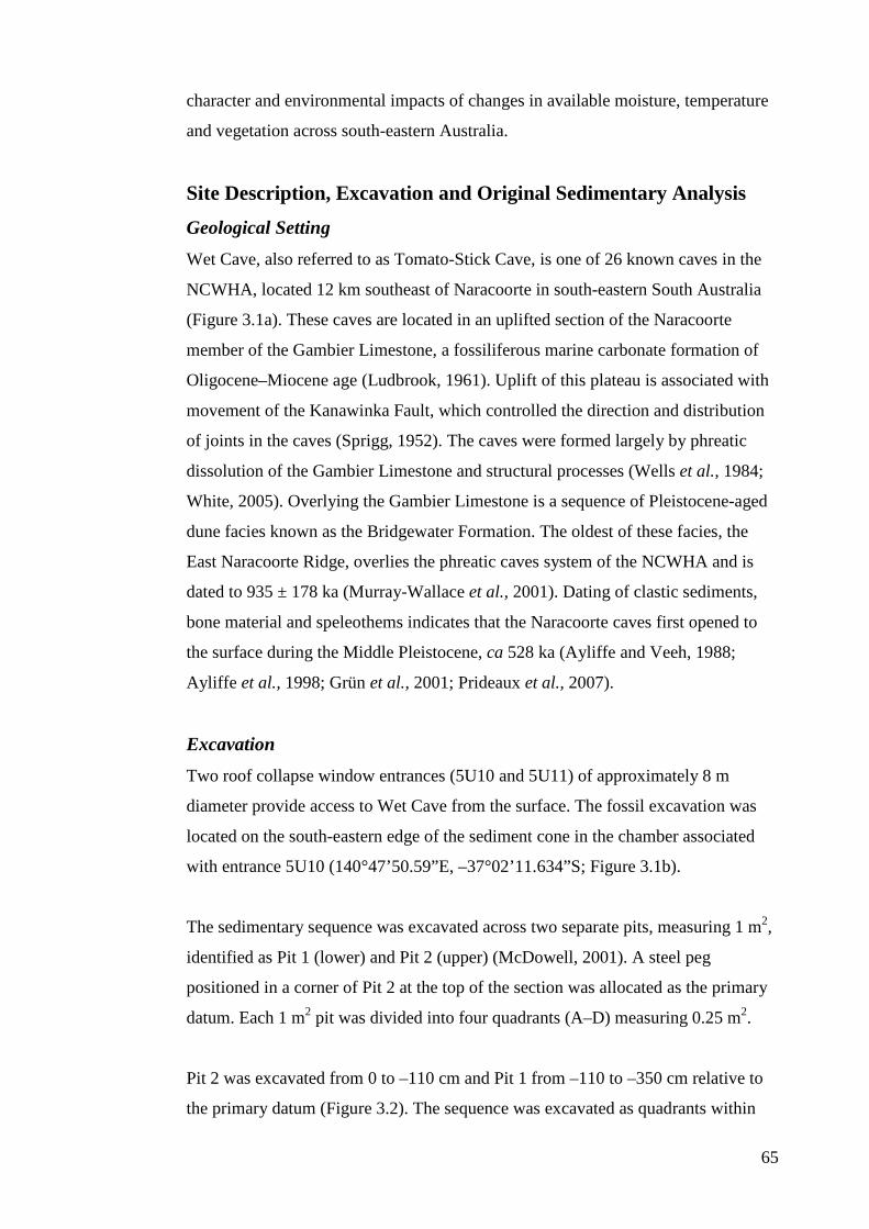
65
character and environmental impacts of changes in available moisture, temperature
and vegetation across south-eastern Australia.
Site Description, Excavation and Original Sedimentary Analysis
Geological Setting Wet Cave, also referred to as Tomato-Stick Cave, is one of 26 known caves in the
NCWHA, located 12 km southeast of Naracoorte in south-eastern South Australia
(Figure 3.1a). These caves are located in an uplifted section of the Naracoorte
member of the Gambier Limestone, a fossiliferous marine carbonate formation of
Oligocene–Miocene age (Ludbrook, 1961). Uplift of this plateau is associated with
movement of the Kanawinka Fault, which controlled the direction and distribution
of joints in the caves (Sprigg, 1952). The caves were formed largely by phreatic
dissolution of the Gambier Limestone and structural processes (Wells et al., 1984;
White, 2005). Overlying the Gambier Limestone is a sequence of Pleistocene-aged
dune facies known as the Bridgewater Formation. The oldest of these facies, the
East Naracoorte Ridge, overlies the phreatic caves system of the NCWHA and is
dated to 935 ± 178 ka (Murray-Wallace et al., 2001). Dating of clastic sediments,
bone material and speleothems indicates that the Naracoorte caves first opened to
the surface during the Middle Pleistocene, ca 528 ka (Ayliffe and Veeh, 1988;
Ayliffe et al., 1998; Grün et al., 2001; Prideaux et al., 2007).
Excavation Two roof collapse window entrances (5U10 and 5U11) of approximately 8 m
diameter provide access to Wet Cave from the surface. The fossil excavation was
located on the south-eastern edge of the sediment cone in the chamber associated
with entrance 5U10 (140°47’50.59”E, –37°02’11.634”S; Figure 3.1b).
The sedimentary sequence was excavated across two separate pits, measuring 1 m2,
identified as Pit 1 (lower) and Pit 2 (upper) (McDowell, 2001). A steel peg
positioned in a corner of Pit 2 at the top of the section was allocated as the primary
datum. Each 1 m2 pit was divided into four quadrants (A–D) measuring 0.25 m2.
Pit 2 was excavated from 0 to –110 cm and Pit 1 from –110 to –350 cm relative to
the primary datum (Figure 3.2). The sequence was excavated as quadrants within
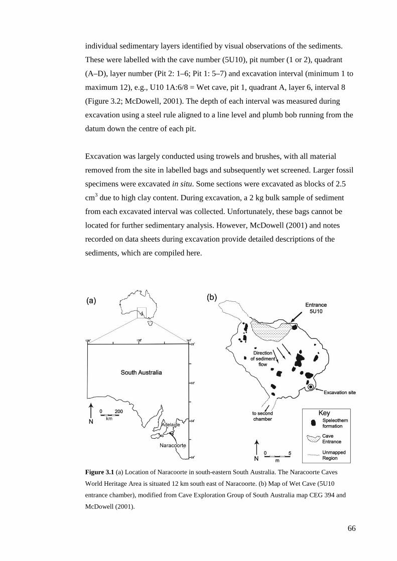
66
individual sedimentary layers identified by visual observations of the sediments.
These were labelled with the cave number (5U10), pit number (1 or 2), quadrant
(A–D), layer number (Pit 2: 1–6; Pit 1: 5–7) and excavation interval (minimum 1 to
maximum 12), e.g., U10 1A:6/8 = Wet cave, pit 1, quadrant A, layer 6, interval 8
(Figure 3.2; McDowell, 2001). The depth of each interval was measured during
excavation using a steel rule aligned to a line level and plumb bob running from the
datum down the centre of each pit.
Excavation was largely conducted using trowels and brushes, with all material
removed from the site in labelled bags and subsequently wet screened. Larger fossil
specimens were excavated in situ. Some sections were excavated as blocks of 2.5
cm3 due to high clay content. During excavation, a 2 kg bulk sample of sediment
from each excavated interval was collected. Unfortunately, these bags cannot be
located for further sedimentary analysis. However, McDowell (2001) and notes
recorded on data sheets during excavation provide detailed descriptions of the
sediments, which are compiled here.
Figure 3.1 (a) Location of Naracoorte in south-eastern South Australia. The Naracoorte Caves
World Heritage Area is situated 12 km south east of Naracoorte. (b) Map of Wet Cave (5U10
entrance chamber), modified from Cave Exploration Group of South Australia map CEG 394 and
McDowell (2001).
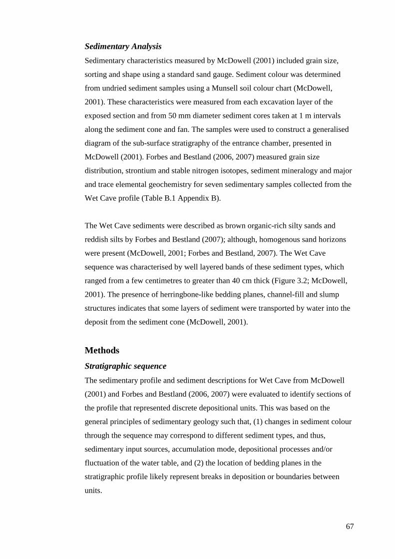
67
Sedimentary Analysis Sedimentary characteristics measured by McDowell (2001) included grain size,
sorting and shape using a standard sand gauge. Sediment colour was determined
from undried sediment samples using a Munsell soil colour chart (McDowell,
2001). These characteristics were measured from each excavation layer of the
exposed section and from 50 mm diameter sediment cores taken at 1 m intervals
along the sediment cone and fan. The samples were used to construct a generalised
diagram of the sub-surface stratigraphy of the entrance chamber, presented in
McDowell (2001). Forbes and Bestland (2006, 2007) measured grain size
distribution, strontium and stable nitrogen isotopes, sediment mineralogy and major
and trace elemental geochemistry for seven sedimentary samples collected from the
Wet Cave profile (Table B.1 Appendix B).
The Wet Cave sediments were described as brown organic-rich silty sands and
reddish silts by Forbes and Bestland (2007); although, homogenous sand horizons
were present (McDowell, 2001; Forbes and Bestland, 2007). The Wet Cave
sequence was characterised by well layered bands of these sediment types, which
ranged from a few centimetres to greater than 40 cm thick (Figure 3.2; McDowell,
2001). The presence of herringbone-like bedding planes, channel-fill and slump
structures indicates that some layers of sediment were transported by water into the
deposit from the sediment cone (McDowell, 2001).
Methods
Stratigraphic sequence The sedimentary profile and sediment descriptions for Wet Cave from McDowell
(2001) and Forbes and Bestland (2006, 2007) were evaluated to identify sections of
the profile that represented discrete depositional units. This was based on the
general principles of sedimentary geology such that, (1) changes in sediment colour
through the sequence may correspond to different sediment types, and thus,
sedimentary input sources, accumulation mode, depositional processes and/or
fluctuation of the water table, and (2) the location of bedding planes in the
stratigraphic profile likely represent breaks in deposition or boundaries between
units.
68
Figure 3.2 Stratigraphic section for Wet Cave, indicating sedimentary and excavation layers
identified by author DNB and described by McDowell (2001). Calibrated radiocarbon dates based on
the INTCAL09 database (Reimer et al., 2009). Ages marked with an asterisk are new dates acquired
in the current study; other ages are calibrated radiocarbon dates from Pate et al., (2002, 2006).
Sedimentary units defined in text. Profile modified from stratigraphic section produced by
McDowell (2001).
69
Radiocarbon Dating In addition to the 14 radiocarbon ages obtained and reported by Pate et al., (2002,
2006; Table 3.1), six additional charcoal samples were selected for further dating of
the site. The additional samples were picked from backup samples sorted from bulk
material excavated during the original work on the deposit. These samples had been
stored since their collection in labelled vials in the Flinders University
Palaeontology Laboratory at the Naracoorte Caves National Park. Samples for
analysis in the current study were selected from excavation intervals for which there
were no existing dates and which would enable greater refinement of the
depositional chronology.
Samples were analysed using AMS radiocarbon dating by Beta Analytic, Florida,
USA, using standard acid/alkali/acid pre-treatment. The conventional radiocarbon
ages of these samples, and the original AMS radiocarbon dates measured for the
site, were calibrated to calendar years BP in OxCal 4.1 (Bronk Ramsey, 2009a)
using the INTCAL09 database (Reimer et al., 2009).
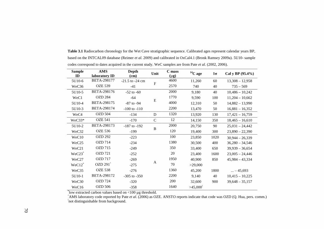
70
Table 3.1 Radiocarbon chronology for the Wet Cave stratigraphic sequence. Calibrated ages represent calendar years BP,
based on the INTCAL09 database (Reimer et al. 2009) and calibrated in OxCal4.1 (Bronk Ramsey 2009a). 5U10- sample
codes correspond to dates acquired in the current study. WeC samples are from Pate et al. (2002, 2006).
Sample ID
AMS laboratory ID
Depth (cm) Unit C mass
(µg) 14C age 1σ Cal y BP (95.4%)
5U10-6 BETA-298177 -21.5 to -24 cm F
4600 11,260 60 13,308 – 12,958 WeC36 OZE 539 -41 2570 740 40 735 – 569 5U10-5 BETA-298176 -52 to -60
E
2000 9,180 40 10,486 – 10,242 WeC1 OZD 284 -64 1770 9,590 100 11,204 – 10,662
5U10-4 BETA-298175 -87 to -94 4000 12,310 50 14,882 – 13,990 5U10-3 BETA-298174 -100 to -110 2200 13,470 50 16,881 – 16,352 WeC4 OZD 504 -134 D 1320 13,920 130 17,421 – 16,759
WeC33* OZE 541 -170 C 12 14,150 350 18,465 – 16,610 5U10-2 BETA-298173 -187 to -192
B 2000 20,750 90 25,031 – 24,442
WeC32 OZE 536 -199 120 19,400 300 23,890 – 22,390 WeC10 OZD 292 -223
A
100 23,850 1020 30,944 – 26,339 WeC25 OZD 714 -234 1380 30,500 400 36,280 – 34,546 WeC21 OZD 715 -249 350 33,400 650 39,939 – 36,654 WeC23* OZD 721 -252 20 23,400 1600 23,005 – 24,446 WeC27 OZD 717 -269 1950 40,900 850 45,984 – 43,334 WeC12* OZD 291^ -275 70 >29,000 WeC35 OZE 538 -276 1360 45,200 1800 ... – 45,693 5U10-1 BETA-298172 -305 to -350 2200 9,140 40 10,415 – 10,225 WeC30 OZD 724 -320 200 32,600 900 39,648 – 35,157 WeC16 OZD 506 -358 1640 >45,000!
*low extracted carbon values based on <100 µg threshold. ^AMS laboratory code reported by Pate et al. (2006) as OZE. ANSTO reports indicate that code was OZD (Q. Hua, pers. comm.) !not distinguishable from background.
71
Results
Sedimentary Sequence and Chronology Sedimentary characteristics through the Wet Cave sequence indicate that it was
composed of a minimum of six sedimentary units (A to F) that are expected to
represent separate episodes of sediment and bone input to the cave (Figure 3.2).
Table B.1 (Appendix B) presents the collated data associated with the sediments
and chronology of the sequence and are summarised in the descriptions below. In
these following descriptions, the depths of each unit within the stratigraphic profile
are reported as depths below the primary datum. The individual layers, which
together compose each sedimentary unit, are also provided. Radiocarbon and
calibrated ages for the Wet Cave sequence are presented in Table 3.1.
Unit A (–350 to –220 cm; Layers 1: 7/9 to 1: 6/12; >45 ka to 30.9–26.3 k Cal y
BP)
Unit A is characterised by dark red, well sorted, sandy clays. The bottom 60 cm of
the unit has a lower sand content than the upper section (McDowell, 2001);
although, SiO2 content is similar for the two sedimentary samples positioned at the
top and bottom of the Unit (sediment samples W10 = 86 wt% and W15 = 91 wt%;
Forbes and Bestland, 2007). By comparison, sample W10 has the highest Al2O3 and
Fe2O3 contents of all samples (6.6 and 2.5 wt%), contrasting with W15, which
contains only 2.6 and 1.3 wt% Al2O3 and Fe2O3, respectively. W15 is distinguished
by a P2O5 content of 0.8 wt%, more than four times higher than any other sample. A
CaO content for W15 of 1.4 wt% contrasts with W10 of only 0.1 wt% (Forbes and
Bestland, 2007) and supports the observations of McDowell (2001) who noted that
limestone fragments were common in the silt and clay layers at the bottom of the
Wet Cave sequence, likely the result of roof-fall and fretting from the cave walls.
This suggests that deposition of the lower unit was relatively slow and is supported
by the radiocarbon chronology for this unit, which spans at least 15,000 years
(Table 3.1).
Despite the geochemical differences between the samples from Unit A, the grain
size distributions are similar (Forbes and Bestland, 2007) and reflect a higher coarse
to fine silt fraction when compared with samples from higher in the sequence, with
the exception of Wp1d (depth –40 cm). However, this sample has a higher medium
72
to fine sand fraction than the samples from Unit A, differentiating it from the lower
sediments.
The mineralogical composition of sedimentary sample W15 (depth –335 cm) shows
that sediments at the bottom of Unit A are composed of 65 vol% clay minerals and
27 vol% quartz, contrasting with samples W2 and Wp1d from Units C and F which
contain 99 and 75 vol% quartz, respectively (Forbes and Bestland, 2007).
One of the additional radiocarbon ages obtained in this study suggests that Layer
1:7/9 (depth –305 to –350 cm) may be of Holocene age (Table 3.1). However, eight
ages reported in Pate et al., (2002, 2006) show that Unit A accumulated in the
Upper Pleistocene. The anomalous age is probably the result of young charcoal
being transported down slope during the paleontological excavation and is not
considered to represent a significant reworking of younger material to the bottom
layer of the sequence. The lack of physical structures in the profile such as cut and
fills, and the consistency of the sedimentary character through Unit A, supports this
assumption.
Unit B (–187 to –220 cm; Layers 1: 6/7 to 1: 6/11; ca 26.3 to 25.0–24.4 k Cal y
BP)
Unit B is characterised by yellow, moderately sorted, polished quartz sands
(McDowell, 2001), bounded by bands of brown clayey sands. Samples W4 and W8
have similar grain size distributions, which vary from other samples being
composed of ~ 56 and 53 vol% very fine sand to coarse silts, respectively (Forbes
and Bestland, 2007). SiO2, Al2O3 and Fe2O3 contents are similar in these samples,
while the concentrations of Zr and Y are identical (Forbes and Bestland, 2007),
supporting the interpretation that they are associated with a single depositional unit.
Unit C (–150 to –187 cm; Layers 1: 6/1 to 1: 6/6; ca 24.4 to ca 18.5–16.6 K Cal y
BP)
Overlying Unit B, from depth –150 cm, is a thick layer of yellow, well sorted,
rounded quartz sand, interspersed with dark brown silty lamina. The grain size
distribution of sample W2 is unique from all other samples, containing ~ 53 vol%
coarse to medium sands with a very low % of silt-sized fractions (Forbes and
73
Bestland, 2007). This sample is composed of 99 vol% quartz (Forbes and Bestland,
2007) and has the lowest Al2O3 and Fe2O3 contents of all samples (1.2 and 0.2 wt%,
respectively). Strontium concentration is also lower in sample W2 than measured in
samples from Units A and B, consistent with the positive correlation between Sr
concentration and silt content observed through the Wet Cave profile (Forbes and
Bestland, 2007).
Unit D (–110 to –150 cm; Layers 1: 5/1 to 1: 5/6)
Overlying Unit C are brown, poorly sorted and sub-rounded clayey sands. Due to
the presence of megafauna fossil remains and similarity in sediment characteristics
with the uppermost and lowermost sections of the profile, McDowell (2001)
suggested that this section of the Wet Cave profile may have been be reworked. The
calibrated age of 17.4–16.8 k cal y BP for charcoal from within this unit (at depth –
134 cm) is broadly consistent with the chronology across the entire sequence but
overlaps the age from Unit C, suggesting a more complex depositional history at
this section of the profile.
Forbes and Bestland (2006) did not investigate the poorly sorted and sub-rounded
clayey sands at the top of Pit 1 and instead described only the homogeneous sands
identified here as Unit C as the “top 60 cm of the Lower Pit” (p. 136). However, the
sedimentary descriptions and profile for Wet Cave provided by McDowell (2001;
Figure 3.2; Table B.1 Appendix B) show that the homogeneous sands extended for
a maximum of 45 cm through the sedimentary profile and clearly indicate the
presence of sediments that are here labelled as Unit D.
Although the discrepancy between the two available descriptions of the Wet Cave
sequence further challenges interpretation of the depositional history of Pit 1, a
photograph of the sequence reported in McDowell (2001) clearly shows the dark
sediments on top of the sands of Unit C. Descriptions of the profile prior to
excavation also note the presence of this layer. It is possible that Forbes and
Bestland (2006) ignored these sediments in their description of the Wet Cave
sequence as they considered it to be a reworked layer as a result of slumping down
the edge of the sedimentary cone. While this interpretation is considered here to be
the most likely explanation for the presence and character of the sediments in Unit
74
D, we have classified and labelled them as a unit to enable a more comprehensive
assessment of the depositional history of the site.
Unit E (–52 to –110 cm; layers 2: 5/1 to 2: 6/4; 16.9–16.3 to 10.5–10.2 k Cal y
BP)
Unit E is characterised by alternating bands of light yellow brown and dark grey,
moderately sorted, sub-rounded clayey and silty sands. The grain size distribution
of sample Wp1h (depth –85 cm) indicates that the dark grey bands are composed of
~ 66 vol% very fine sands to coarse silts, contrasting with all other samples. The
uppermost band of Unit E contains limestone gravel suggesting a depositional
hiatus occurred from ca 10.5–10.2 k cal y BP.
Unit F (0 to –52 cm; Layers 2: 1/1 to 2: 4/1; Holocene age; containing some
reworked material from Unit E)
The uppermost unit of the deposit was characterised by very dark grey to very dark
brown, moderately sorted, sub-rounded silty sands, interposed with clean sandy
lamina (McDowell, 2001). The boundary between Units E and F was indicated by
the presence of flowstone at depth –39 to –52 cm (McDowell, 2001); although it is
unknown if the flowstone was attached to the cave wall or free floating. The grain
size distribution and geochemistry of sample Wp1d (depth –40 cm) contrasts with
all other samples, indicating the unique composition of sediments at this part of the
profile.
As noted by Forbes and Bestland (2006), the sample incorporated a milky white
non-clastic material not observed elsewhere in the profile. Wp1d is characterised by
very low SiO2 content; although, this does not correlate with high Al2O3 and Fe2O3
contents as would be expected based on the strong linear correlation of these oxides
with SiO2 in the other samples. As noted by Forbes and Bestland (2006), high LOI
(5.8 wt%) and CaO (11.9 wt%) contents in combination with a SO3 content of 15.3
wt% suggests bat guano contributions to these sediments. The presence of bat
guano at this section of the profile in addition to the flowstone indicates minimal
allogenic inputs for a period of time prior to the deposition of the largely Holocene-
aged dark brown silts and sub-rounded quartz laminations.
75
The calibrated radiocarbon age of a charcoal sample from layer 2:2/3 (depth –21.5
to –24 cm; 13.3–13.0 k cal y BP) suggests possible reworking of Pleistocene
material from Unit E, likely via natural post-depositional processes and
anthropogenic disturbance as evidenced by the presence of European artifacts (e.g.,
ceramic and glass shards) recovered from sediments in Pit 2.
Discussion
Relationship to other Upper Pleistocene sequences of the NCWHA The Wet Cave sedimentary and fossil sequence spans ca 45,000 years, providing a
record of the latter part of Last Glacial Cycle and Holocene for the NCWHA. While
the deposit is broadly contemporaneous with the inner chamber deposit of
Robertson Cave 5U17 (RCIC), located approximately 6 km south of Wet Cave, the
Wet Cave sequence is more continuous and contains sediments dated to the last
glacial maximum (LGM; ca, 20–17 ka; Barrows et al., 2002) which are absent from
RCIC (Forbes et al., 2007). Radiocarbon ages for the 3rd chamber deposit in
Blanche Cave 5U6 (BC3C), located within 400 m of Wet Cave, show that it also
contains an LGM sequence, but does not contain in situ Holocene aged material (St
Pierre et al., 2012). Hence, Wet Cave is an important sequence for the NCWHA,
providing a record of temporal periods not represented elsewhere and a sequence
against which environmental and paleoclimatic signals interpreted from other Upper
Pleistocene deposits may be compared.
The identification of six sedimentary units, including the reworked Unit D, within
the Wet Cave sequence compares well with BC3C where five units, plus a reworked
layer, were identified from a stratigraphic core (Darrénougué et al., 2009).
Available chronological data (Darrénougué et al., 2009; St Pierre et al., 2012)
suggest that the analogous units identified in the two caves are broadly
contemporaneous and may be used to assess local paleoenvironmental
interpretations for the Upper Pleistocene based on the sediments from a single
deposit (e.g., Darrénougué et al., 2009).
Despite similarities in the character of the sedimentary units between the Wet Cave
and BC3C deposits, the depth profiles of the sequences are quite different. This
variation is expected to reflect local accumulation and post-depositional processes
76
associated with the shape and structure of the cave chambers, entrances and surface
topography. Such processes are expected to also account for the differences in the
composition and temporal span of the sedimentary sequences of Wet Cave and
RCIC, which is composed of only three units; Lower, Middle and Upper (Forbes et
al., 2007). These units share similar characteristics respectively with Units A, B and
E of the Wet Cave sequence and their analogues in BC3C.
The sources of sediments that fill Wet Cave were first inferred by McDowell (2001)
and later expanded by Forbes and Bestland (2007) using geochemical assessment of
surficial and NCWHA sediments. Correlations identified by Forbes and Bestland
(2007) generally supported the interpretations of McDowell (2001) and previous
researchers (e.g., Wells et al., 1984; Moriarty et al., 2000). The proximal sources of
clays and silts to the NCWHA deposits were found to be the medium–silt sized
fractions of local Terra Rossa Soils, while sands were largely derived from the
sandy A horizon of Coonawarra Terra Rossa Soils, and the medium-grained sands
of the coastal barrier dunes, the Bridgewater Formation (Forbes and Bestland,
2007). It is interesting to note that there was poor geochemical correlation with the
coarser-grained, calcite-rich component of the Bridgewater Formation. This
suggests that carbonate grains and cement of the Bridgewater Formation had been
dissolved leaving the medium-grained quartz component free to be transported
around the landscape. Finally, the organic-rich sediments from Wet Cave Unit F
were correlated with local Holocene podsols and/or anthropogenically disturbed
soils (McDowell, 2001; Forbes and Bestland, 2007).
Paleoclimatic Context McDowell (2001) summarised a depositional and environmental history for the
NCWHA from the Wet and RCIC sequences. In light of the refined chronology and
sedimentary sequence for Wet Cave, the paleoclimatic context of the deposit is re-
examined here. This assessment also utilises more recent literature and proxy data
for Upper Pleistocene climates in south-eastern Australia. The chronology for
marine isotope stages follows Martinson et al., (1987) with age refinements for
MIS-2 and MIS-3 sub-stages from Thompson and Goldstein (2006).
77
Unit A: MIS-3
The calibrated radiocarbon chronology for Wet Cave indicates that the red-brown
sandy clays of Unit A accumulated during MIS-3. On the basis of apparent full lake
levels in the Willandra region of the south-eastern Australian Mallee, Darrénougué
et al., (2009) suggested that the MIS-3 aged unit of BC3C accumulated during a
very wet climatic phase. However, a broader review of paleoclimatic data for this
period suggests more temporally and spatially variable climatic conditions during
the deposition of the red-brown clays in BC3C, and hence Wet Cave at this time.
Cool conditions relative to today during MIS-3 are evident in the global oxygen
isotope SPECMAP curve which indicates a gradual decline in global temperatures
prior to the LGM depression (Martinson et al., 1987). Regional sea surface
temperatures reconstructed using alketones in Murray Canyons core MD03-2607
also show cooler temperatures than today, and reveal frequent fluctuations within
the range of ca. 12–17°C during MIS-3 (Lopes dos Santos et al., 2012). Episodic
high fluvial activity through the rivers of the Riverine Plain suggests pluvial
conditions during MIS-3 in south-eastern Australia is consistent with this
fluctuation, with two primary phases identified at ca 55–35 ka (Kerabury Phase)
and ca 35–25 ka (Gum Creek Phase) (Page et al., 1996, 2001). These phases of high
episodic flows have been linked with periods of glaciation and periglacial
conditions in the Snowy Mountains that feed the Riverine Plain; a lower snowline is
expected to have increased the volume of winter snowpack and hence, snowmelt
during spring (Barrows et al., 2001). The episodic/seasonal nature of large flows of
the Riverine Plain is evidenced by the near synchronous ages of source-bordering
dunes, indicating deflation from the paleochannels during periods of low flow and
higher evaporation (Page et al., 2001; Kemp and Spooner, 2007).
A fine scale review of the water level record for the Willandra system shows that
MIS-3 was characterised by fluctuation between phases of higher and lower
lacustral activity (lake levels), correlated with lesser and greater pelletal clay dune
building indicative of drier periods (Bowler, 1998; Bowler et al., 2007, 2012). The
early phase of sedimentation of Unit A into Wet Cave coincides with a pre-LGM
glacial advance in Tasmania at ca 45–40 ka (Barrows et al., 2002; Mackintosh et
al., 2006), coincident with transition from a phase of high water level at ca 44–42
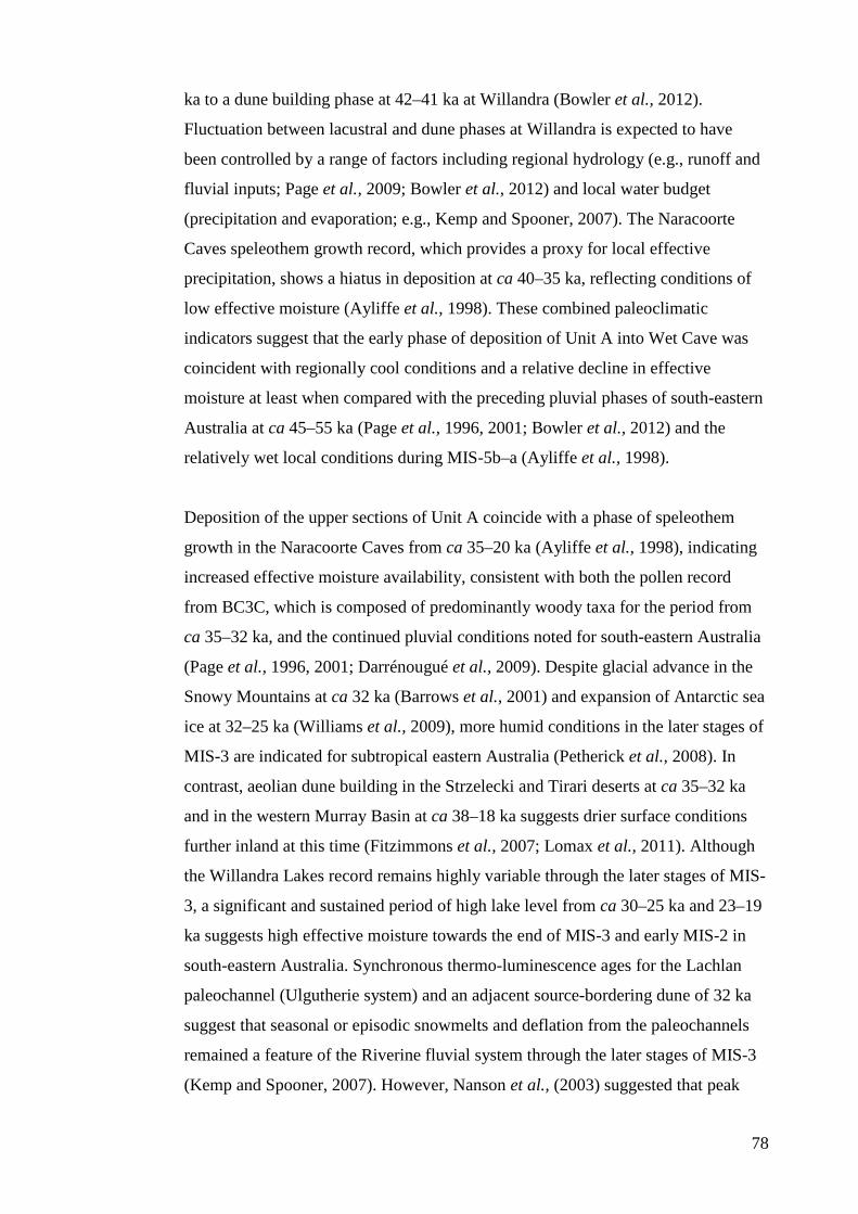
78
ka to a dune building phase at 42–41 ka at Willandra (Bowler et al., 2012).
Fluctuation between lacustral and dune phases at Willandra is expected to have
been controlled by a range of factors including regional hydrology (e.g., runoff and
fluvial inputs; Page et al., 2009; Bowler et al., 2012) and local water budget
(precipitation and evaporation; e.g., Kemp and Spooner, 2007). The Naracoorte
Caves speleothem growth record, which provides a proxy for local effective
precipitation, shows a hiatus in deposition at ca 40–35 ka, reflecting conditions of
low effective moisture (Ayliffe et al., 1998). These combined paleoclimatic
indicators suggest that the early phase of deposition of Unit A into Wet Cave was
coincident with regionally cool conditions and a relative decline in effective
moisture at least when compared with the preceding pluvial phases of south-eastern
Australia at ca 45–55 ka (Page et al., 1996, 2001; Bowler et al., 2012) and the
relatively wet local conditions during MIS-5b–a (Ayliffe et al., 1998).
Deposition of the upper sections of Unit A coincide with a phase of speleothem
growth in the Naracoorte Caves from ca 35–20 ka (Ayliffe et al., 1998), indicating
increased effective moisture availability, consistent with both the pollen record
from BC3C, which is composed of predominantly woody taxa for the period from
ca 35–32 ka, and the continued pluvial conditions noted for south-eastern Australia
(Page et al., 1996, 2001; Darrénougué et al., 2009). Despite glacial advance in the
Snowy Mountains at ca 32 ka (Barrows et al., 2001) and expansion of Antarctic sea
ice at 32–25 ka (Williams et al., 2009), more humid conditions in the later stages of
MIS-3 are indicated for subtropical eastern Australia (Petherick et al., 2008). In
contrast, aeolian dune building in the Strzelecki and Tirari deserts at ca 35–32 ka
and in the western Murray Basin at ca 38–18 ka suggests drier surface conditions
further inland at this time (Fitzimmons et al., 2007; Lomax et al., 2011). Although
the Willandra Lakes record remains highly variable through the later stages of MIS-
3, a significant and sustained period of high lake level from ca 30–25 ka and 23–19
ka suggests high effective moisture towards the end of MIS-3 and early MIS-2 in
south-eastern Australia. Synchronous thermo-luminescence ages for the Lachlan
paleochannel (Ulgutherie system) and an adjacent source-bordering dune of 32 ka
suggest that seasonal or episodic snowmelts and deflation from the paleochannels
remained a feature of the Riverine fluvial system through the later stages of MIS-3
(Kemp and Spooner, 2007). However, Nanson et al., (2003) suggested that peak
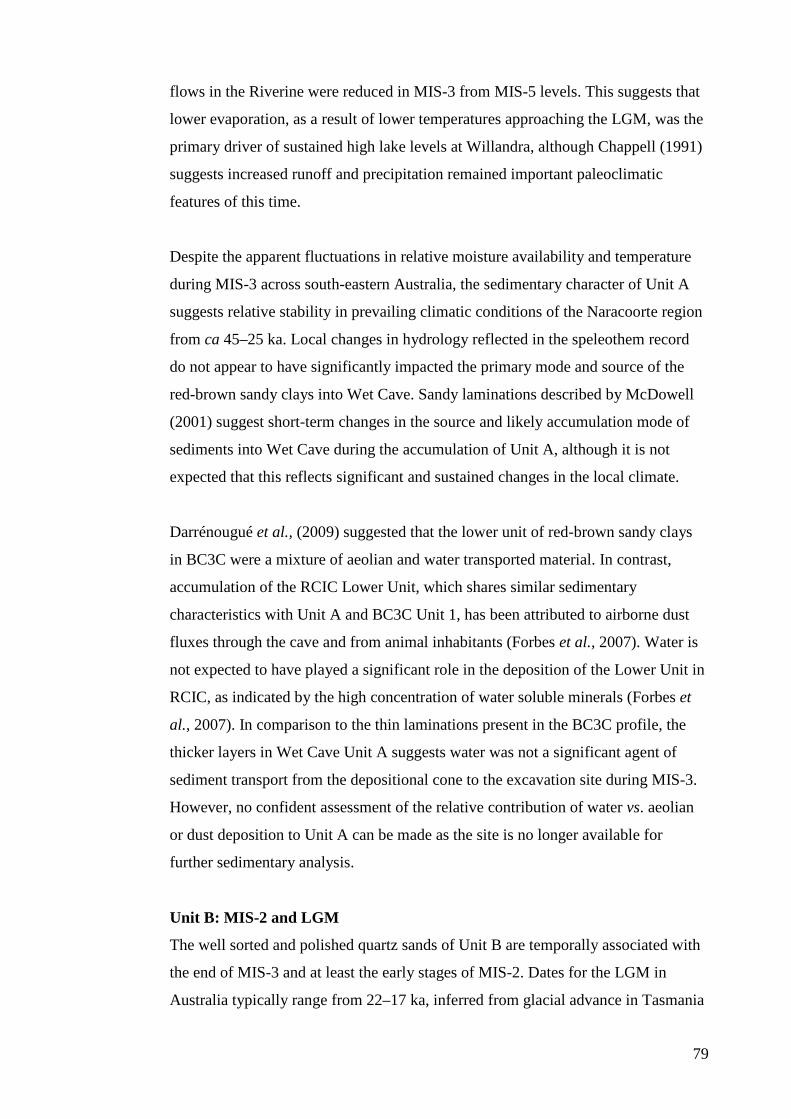
79
flows in the Riverine were reduced in MIS-3 from MIS-5 levels. This suggests that
lower evaporation, as a result of lower temperatures approaching the LGM, was the
primary driver of sustained high lake levels at Willandra, although Chappell (1991)
suggests increased runoff and precipitation remained important paleoclimatic
features of this time.
Despite the apparent fluctuations in relative moisture availability and temperature
during MIS-3 across south-eastern Australia, the sedimentary character of Unit A
suggests relative stability in prevailing climatic conditions of the Naracoorte region
from ca 45–25 ka. Local changes in hydrology reflected in the speleothem record
do not appear to have significantly impacted the primary mode and source of the
red-brown sandy clays into Wet Cave. Sandy laminations described by McDowell
(2001) suggest short-term changes in the source and likely accumulation mode of
sediments into Wet Cave during the accumulation of Unit A, although it is not
expected that this reflects significant and sustained changes in the local climate.
Darrénougué et al., (2009) suggested that the lower unit of red-brown sandy clays
in BC3C were a mixture of aeolian and water transported material. In contrast,
accumulation of the RCIC Lower Unit, which shares similar sedimentary
characteristics with Unit A and BC3C Unit 1, has been attributed to airborne dust
fluxes through the cave and from animal inhabitants (Forbes et al., 2007). Water is
not expected to have played a significant role in the deposition of the Lower Unit in
RCIC, as indicated by the high concentration of water soluble minerals (Forbes et
al., 2007). In comparison to the thin laminations present in the BC3C profile, the
thicker layers in Wet Cave Unit A suggests water was not a significant agent of
sediment transport from the depositional cone to the excavation site during MIS-3.
However, no confident assessment of the relative contribution of water vs. aeolian
or dust deposition to Unit A can be made as the site is no longer available for
further sedimentary analysis.
Unit B: MIS-2 and LGM
The well sorted and polished quartz sands of Unit B are temporally associated with
the end of MIS-3 and at least the early stages of MIS-2. Dates for the LGM in
Australia typically range from 22–17 ka, inferred from glacial advance in Tasmania
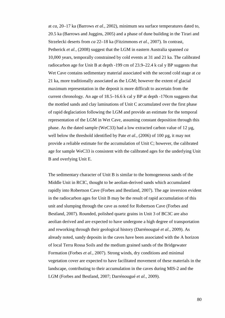
80
at ca, 20–17 ka (Barrows et al., 2002), minimum sea surface temperatures dated to,
20.5 ka (Barrows and Juggins, 2005) and a phase of dune building in the Tirari and
Strzelecki deserts from ca 22–18 ka (Fitzimmons et al., 2007). In contrast,
Petherick et al., (2008) suggest that the LGM in eastern Australia spanned ca
10,000 years, temporally constrained by cold events at 31 and 21 ka. The calibrated
radiocarbon age for Unit B at depth -199 cm of 23.9–22.4 k cal y BP suggests that
Wet Cave contains sedimentary material associated with the second cold stage at ca
21 ka, more traditionally associated as the LGM; however the extent of glacial
maximum representation in the deposit is more difficult to ascertain from the
current chronology. An age of 18.5–16.6 k cal y BP at depth -170cm suggests that
the mottled sands and clay laminations of Unit C accumulated over the first phase
of rapid deglaciation following the LGM and provide an estimate for the temporal
representation of the LGM in Wet Cave, assuming constant deposition through this
phase. As the dated sample (WeC33) had a low extracted carbon value of 12 µg,
well below the threshold identified by Pate et al., (2006) of 100 µg, it may not
provide a reliable estimate for the accumulation of Unit C; however, the calibrated
age for sample WeC33 is consistent with the calibrated ages for the underlying Unit
B and overlying Unit E.
The sedimentary character of Unit B is similar to the homogeneous sands of the
Middle Unit in RCIC, thought to be aeolian-derived sands which accumulated
rapidly into Robertson Cave (Forbes and Bestland, 2007). The age inversion evident
in the radiocarbon ages for Unit B may be the result of rapid accumulation of this
unit and slumping through the cave as noted for Robertson Cave (Forbes and
Bestland, 2007). Rounded, polished quartz grains in Unit 3 of BC3C are also
aeolian derived and are expected to have undergone a high degree of transportation
and reworking through their geological history (Darrénougué et al., 2009). As
already noted, sandy deposits in the caves have been associated with the A horizon
of local Terra Rossa Soils and the medium grained sands of the Bridgewater
Formation (Forbes et al., 2007). Strong winds, dry conditions and minimal
vegetation cover are expected to have facilitated movement of these materials in the
landscape, contributing to their accumulation in the caves during MIS-2 and the
LGM (Forbes and Bestland, 2007; Darrénougué et al., 2009).
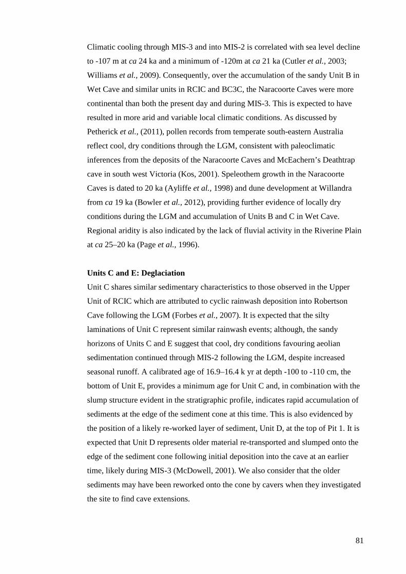
81
Climatic cooling through MIS-3 and into MIS-2 is correlated with sea level decline
to -107 m at ca 24 ka and a minimum of -120m at ca 21 ka (Cutler et al., 2003;
Williams et al., 2009). Consequently, over the accumulation of the sandy Unit B in
Wet Cave and similar units in RCIC and BC3C, the Naracoorte Caves were more
continental than both the present day and during MIS-3. This is expected to have
resulted in more arid and variable local climatic conditions. As discussed by
Petherick et al., (2011), pollen records from temperate south-eastern Australia
reflect cool, dry conditions through the LGM, consistent with paleoclimatic
inferences from the deposits of the Naracoorte Caves and McEachern’s Deathtrap
cave in south west Victoria (Kos, 2001). Speleothem growth in the Naracoorte
Caves is dated to 20 ka (Ayliffe et al., 1998) and dune development at Willandra
from ca 19 ka (Bowler et al., 2012), providing further evidence of locally dry
conditions during the LGM and accumulation of Units B and C in Wet Cave.
Regional aridity is also indicated by the lack of fluvial activity in the Riverine Plain
at ca 25–20 ka (Page et al., 1996).
Units C and E: Deglaciation
Unit C shares similar sedimentary characteristics to those observed in the Upper
Unit of RCIC which are attributed to cyclic rainwash deposition into Robertson
Cave following the LGM (Forbes et al., 2007). It is expected that the silty
laminations of Unit C represent similar rainwash events; although, the sandy
horizons of Units C and E suggest that cool, dry conditions favouring aeolian
sedimentation continued through MIS-2 following the LGM, despite increased
seasonal runoff. A calibrated age of 16.9–16.4 k yr at depth -100 to -110 cm, the
bottom of Unit E, provides a minimum age for Unit C and, in combination with the
slump structure evident in the stratigraphic profile, indicates rapid accumulation of
sediments at the edge of the sediment cone at this time. This is also evidenced by
the position of a likely re-worked layer of sediment, Unit D, at the top of Pit 1. It is
expected that Unit D represents older material re-transported and slumped onto the
edge of the sediment cone following initial deposition into the cave at an earlier
time, likely during MIS-3 (McDowell, 2001). We also consider that the older
sediments may have been reworked onto the cone by cavers when they investigated
the site to find cave extensions.
82
The thicker and more defined alternating sand-clay laminations of Unit E may
correspond to greater fluctuation in paleoenvironmental or climatic conditions
locally and more regionally during the LGM deglaciation. Initial assessment of the
ages of the yellow-brown sandy clays suggests ca 2,000 year intervals between
deposition of these layers. These laminations are similar to the sequence described
in Unit 4 of BC3C; however, the internal chronology for Unit 4 reflects post
depositional disturbance and mixing of the sedimentary layers in this section of the
BC3C deposit (St Pierre et al., 2012), whereas there is no evidence for disturbance
in Unit E of Wet Cave.
Warming following the cold-dry glacial conditions of the LGM across south-eastern
Australia is variable: an initial phase of deglaciation is evidenced in rapid sea level
rise over a few hundred years from 19 ka (Yokoyama et al., 2000) and warming of
oceans off the South Australian coast at ca 19–15.5 ka (Calvo et al., 2007).
However, regional variation in prevailing conditions is apparent with short term
glacial advances in the Snowy Mountains at ca 19 ka and 17 ka (Barrows et al.,
2002). In south-eastern South Australia, dry conditions prevailed to the Holocene as
indicated in the pollen and sedimentation records of Lake Leake and Wyrie Swamp
(Dodson, 1975, 1977), the persistence of steppe-grasslands with low tree cover from
ca 18 ka to the Holocene (ca 11.5 ka) in western Victoria (Kershaw et al., 2004)
and erosional deflation of Lakes Bolac and Turangmoroke, also in western Victoria
between 18 and 11 ka (Cook, 2009). Pollen sequences from the Basalt Plains of
western Victoria also suggests that lowest rainfall in the region was experienced at
ca 14–12 ka rather than at the LGM (D’Costa et al., 1989; Kershaw et al., 2004),
but is expected to be a function of increased evaporation with rising temperatures.
This phase of maximum aridity is coincident with a post LGM phase of dune
building in the Strzelecki and Tirari deserts from 14–10 ka (Fitzimmons et al.,
2007) and the Antarctic cold reversal at ca 14.5–13 ka (Jouzel et al., 1995). The
evolution of modern flow regimes associated with reduced flows and greater
suspended loads on the Riverine Plain is dated from ca 12 ka, coinciding with
reduction in the periglacial zone and elevation of the treeline which reduced the
amount of debris and melt flows from the Snowy Mountains (Page et al., 2009) and
a second phase of post LGM warming dated from ca 13.3–11 ka (Calvo et al.,
2007).
83
Relatively dry conditions at the Naracoorte Caves during the LGM deglaciation are
indicated by lack of speleothem growth from 20 ka (Ayliffe et al., 1998). A Local
increase in effective moisture is not indicated until ca 10 ka, as reflected in the
pollen records of Lake Leake and Wyrie Swamp (Dodson, 1975, 1977). In contrast,
high fluvial activity on the Riverine Plain from 20–13 ka suggests the maintenance
of a seasonal positive water budget through the LGM deglaciation, likely associated
with increased effective moisture and runoff from snowpack and glaciers associated
with the late glacial advances at ca 19 and 17 ka in the Snowy Mountains (Page et
al., 2009).
Unit F: Holocene
Unit F contains Holocene aged material (dated to 0.7–0.6 k cal y BP) that is
expected to have accumulated following a depositional hiatus of unknown duration,
evidenced by the presence of a flowstone and layer of bat guano at depth -52 cm
(McDowell, 2001; Forbes and Bestland, 2007). The high concentration of SO3 in
sediment sample Wp1d (Forbes and Bestland, 2006) suggests that the top of the
profile remained relatively dry through the last ca 750 years, consistent with
observed dry conditions in the late Holocene as reflected in regional pollen records
(e.g., D’Costa et al., 1989; Kershaw et al., 2004; Cook, 2009). However, Dodson
and Mooney’s (2002) review of changes in Holocene temperatures and effective
moisture, and a recent study of the Willandra Lakes (Kemp et al., 2012), suggest
greater temporal and spatial variation in these parameters than noted here. It is not
possible to temporally constrain the growth period associated with the flowstone
noted from the Wet Cave sequence; however, it is expected that it is older than the
Holocene aged sediments of Unit F and represents climatic conditions or a phase of
higher effective moisture than represented by sediment sample Wp1d.
Human disturbance to the upper layers of the BC3C deposit is evident in the poor
chronological consistency noted by Darrénougué et al., (2009) and St Pierre et al.,
(2012). McDowell (2001) suggested that Wet Cave contains a pre-European record
of the local fauna but identified the very top layer of sediment as reworked based on
the presence of orange clays and European artifacts. Further radiocarbon dating
suggests that the sediments of Unit F may contain material of a mixture of
84
Pleistocene and Holocene ages, cautioning paleoecological interpretation of the
faunas from Unit F (Table 3.1).
Environmental changes associated with European arrival, measured in sedimentary
and pollen deposits of eastern Australia, commonly show increased sedimentation
and vegetation change at rates higher than recorded from pre-European sequences
(Dodson and Mooney, 2002). Darrénougué et al., (2009) found no correlation
between the thin layer of dark, organic matter-rich sediment at the top of the BC3C
sediment core (Unit 5) and regional/local surface deposits and suggested that it
represents a unique depositional episode, likely associated with human activity. In
contrast, McDowell (2001) and Forbes and Bestland (2007) suggested that the dark,
organic matter-rich Holocene aged silty sands within the Naracoorte Caves were
derived from local podsols. Forbes et al., (2007) suggested that the high organic
matter and charcoal content of the early Holocene aged material in RCIC reflects
climatic warming and wetting following the LGM, an inference supported by δ13C
isotopic data from charcoal and soil organic matter measured from RCIC. As the
upper unit in Wet Cave is younger than the Upper Unit of RCIC, it is expected that
Wet Cave provides a record of changed conditions from the early, warm and wet
phase of the Holocene to drier conditions associated with higher temperatures and
increased impacts of human activity on the surrounding landscape.
Conclusions Collation of stratigraphic and sedimentary data collected during past studies of Wet
Cave has enabled a review of the stratigraphy and paleoclimatic and environmental
signals for the Upper Pleistocene–Holocene from this deposit. Five in situ and one
reworked sedimentary unit have been identified in the Wet Cave sequence, each
representing depositional episodes correlated with changes in paleoclimatic
conditions of the Last Glacial Cycle in south-eastern Australia, spanning from mid
MIS-3 to the Holocene. Additional radiocarbon ages have provided further
constraints on the age of some units and have revealed possible re-worked areas in
the sequence. This review of the Wet Cave sequence and its paleoclimatic context
provides a basis for future investigation of the Wet Cave fossil assemblage and
environmental record. It was also critical for enabling the Wet Cave assemblage to
85
be correlated with contemporaneous records from other caves within the NCWHA
in order to test the paleoecological signals interpreted from a single deposit.
Acknowledgements This review of the Wet Cave sedimentary sequence and additional radiocarbon
dating would not have been possible without the extensive work of Matt Forbes,
Erick Bestland, Donald Pate, Simone Dalgairns and students of the 1997 and 1998
Vertebrate Paleontology course of Flinders University. Their contributions to the
systematic collection of fossils, charcoal and sedimentary and chronological data
from the site have proved invaluable as the site is now longer available for further
analysis. Radiocarbon dating was funded by EHR and a Betty Mayne Scientific
Research Grant from the Linnean Society of New South Wales awarded to ACM.
We extend warm thanks to Drs Quan Hua and Donald Pate for providing additional 14C data associated with the original dating samples and to Drs Erick Bestland,
Patrick DeDeckker and Anita Andrew for comments which improved the
manuscript.
86
4. Bayesian age-depth modelling of Late Quaternary
deposits from Wet and Blanche Caves, Naracoorte, South
Australia: a framework for comparative faunal analyses
Citation Macken, A.C., Staff, R.A. and Reed, E.H. (2013) Bayesian age-depth modelling of
Late Quaternary deposits from Wet and Blanche Caves, Naracoorte, South
Australia: a framework for comparative faunal analyses. Quaternary
Geochronology 17, 26–43.
Contribution of Authors Amy Macken:
• Devised and planned the project.
• Compiled stratigraphic and chronological data that were integrated into the
models.
• Worked closely with RS to develop the models.
• Prepared the manuscript for publication with the support of RS.
Richard Staff:
• Developed the models in OxCal.
• Supported AM with preparation of the manuscript.
Elizabeth Reed:
• Provided stratigraphic data for Blanche Cave.
• Assisted with the stratigraphic interpretation of the Blanche Cave sequence
for the purpose of age modelling.
• Provided comments on the manuscript.
87
Signed .................................................................................. Date ............................
Amy Macken
School of Biological Sciences, Flinders University
Signed .................................................................................. Date ............................
Richard Staff
Oxford Radiocarbon Accelerator Unit, Research Laboratory for Archaeology and
the History of Art, University of Oxford
Signed .................................................................................. Date ............................
Elizabeth Reed
School of Biological Sciences, Flinders University

88
Abstract Bayesian age-depth models were constructed for two Late Quaternary aged fossil-
bearing sedimentary sequences from caves in south eastern South Australia. The
deposits in Wet and Blanche Caves contain dense assemblages of vertebrate fossils,
largely the result of owl pellet accumulation. While individually calibrated
radiocarbon determinations from the fossil sequences have provided a chronology
for their accumulation, there was limited capacity available with such data to (a)
temporally constrain assemblages associated with different depositional units and
layers within the two sites, (b) interpret the chronological relationships among
successive units and layers and (c) correlate sedimentary units and layers of similar
age between the two deposits. Here, Bayesian age-depth models were constructed in
OxCal for the Wet and Blanche Cave sequences, incorporating the available
radiocarbon data and stratigraphic information collected during their excavation.
Despite the low precision of the age-depth models for Wet and Blanche Caves
which results in part from there being only single radiocarbon determinations
available for a number of units and layers, the models enabled the relationships
within and between the two sites to be established. Of particular utility for future
faunal analyses is quantification of the temporal relationship between strata from
the two sites, where groups of individual layers from Blanche Cave were found to
be temporally equivalent with the longer-duration units in Wet Cave. We suggest
that the use of Phase modelling, as performed here, is useful for cave deposits that
have complex depositional histories and even in such instances where, as is
common for palaeontological sites, few radiocarbon data are collected relative to
the time-spans of tens of millennia that are often represented by them.
Keywords 14C dating, age-depth modelling, Bayesian statistics, cave sequence, last
glacial cycle, Naracoorte Caves
Introduction The utility of radiocarbon (14C) dating to provide chronologies for late Quaternary
aged archaeological and palaeontological sites is well demonstrated (e.g., Gillespie,
2002; Vasil’ev et al., 2002; Crowley, 2010). However, sparse radiocarbon data and
statistical uncertainty often restrict the resolution and accuracy of site chronologies
based on individually calibrated 14C determinations (Parnell et al., 2011). Bayesian
89
chronological methods can overcome these limitations and have increasingly been
used to develop chronologies for palaeontological and archaeological sites where a
high level of dating precision is required (e.g., Petrie and Torrence, 2008;
Beramendi-Orosco et al., 2009; Calcagnile et al., 2010; Higham et al., 2010; Zhu et
al., 2010). By integrating 14C data (likelihoods) and stratigraphic information
(priors), Bayesian age-depth models produce posterior (modelled) site chronologies
that not only refine the chronological information available for a given sequence,
but also provide quantified uncertainties for such profiles, given the model prior
applied (Bronk Ramsey, 2008; Parnell et al., 2011). As demonstrated by Blaauw et
al. (2007), Bayesian age-depth models can also be used to temporally correlate the
proxy records from contemporaneous sequences. While correlation of depositional
sequences commonly utilises stratigraphic, sedimentary and chronological data
(e.g., Birkland et al., 1971; Magee et al., 1995; Frumkin et al., 2001), these past
approaches have rarely taken account of the underlying chronological uncertainties
both within and between records.
Cave sites are particularly important in Quaternary palaeontological studies as they
contain deep, well stratified sedimentary sequences often spanning multiple
millennia (e.g., Cuenca-Bescos et al., 2009). Caves also provide stable conditions
for the long term preservation of skeletal remains of a diverse range of vertebrates,
which may have been collected through pitfall entrapment, cave inhabitant death
and/or carnivore accumulation (Nielsen-Marsh, 2000). In some cases, vertebrate
deposits in caves are associated with a range of other palaeoecological materials
such as charcoal, calcium carbonate cave formations (speleothems) and pollen,
which may be correlated with fossil faunal assemblages to provide a more accurate
interpretation of past environmental conditions (e.g., Burney et al., 2001; Carrión et
al., 2003; Auler et al., 2006). The application of Bayesian age-depth models to cave
sequences has been valuable where the complex and sometimes random nature of
accumulation processes in caves can limit the resolution and accuracy of
chronologies for these sites (e.g., Jacobi and Higham, 2009; Blockey and Pinhasi,
2011; Pinhasi et al., 2011).
In south eastern South Australia, 26 caves within the Naracoorte Caves complex
contain 100 known vertebrate fossil deposits ranging from early Pleistocene to
90
Holocene age (Reed and Bourne, 2000; Prideaux et al., 2007; Macken et al., 2013a;
Fig. 4.1). Within this cave complex, deposits in two of these caves, Wet and
Blanche, are broadly contemporaneous, spanning the late Pleistocene from ca. 45
ka, to the Holocene period (Darrénougué et al., 2009; St. Pierre et al., 2012;
Macken et al., 2013a). Fine stratigraphic laminations contained within broader
sedimentary units in these cave sequences, in combination with the high density of
bone material identified from these deposits (McDowell, 2001; Laslett, 2006;
Macken and Reed, 2013) makes them suitable for the analysis of faunal patterns
through the last glacial cycle at a range of temporal scales, incorporating both long
and short term phases of accumulation. As these sites are of similar age, they also
provide an opportunity to quantify inter-site variability within the palaeocommunity
through similarity tests of contemporaneous, replicate fossil samples from the one
locality, an approach endorsed by Bennington and Bambach (1996).
Data on the calibrated age, duration and temporal continuity of depositional units
and layers of the fossil bearing sedimentary profiles of Wet and Blanche Caves are
required to temporally constrain the faunal assemblages and to enable an evaluation
of faunal change through time, both within and between the two sites. To facilitate
such analyses, greater chronological resolution is required than has been previously
published. In the case of Wet Cave, only a small number of 14C determinations are
available (Macken et al., 2013a; Table 4.1). In Blanche Cave, although more 14C
determinations are available for the sequence (St Pierre et al., 2012; Table 4.2),
overlap in the calibrated radiocarbon ages of successive layers limits the resolution
at which faunal analyses may be conducted.
Here, we use Bayesian age-depth models to assess the chronological histories of
Wet and Blanche Cave and the temporal relationships between strata from the two
sites. As fossil-bearing deposits, understanding these relationships is critical for
robust and informed comparative faunal analyses. More specifically we use
Bayesian age-depth modelling to (a) construct probabilistic site chronologies that
provide modelled ages for the lower and upper boundaries (reflecting the start and
end) of depositional episodes (stratigraphic units and finer sedimentary layers)
within the two sequences, (b) determine the temporal duration (resolution) of these
depositional episodes and potential hiatuses between them, and (c) identify
91
contemporaneous depositional episodes between the two sites. We discuss the
challenges and opportunities presented by such models for the study of complex
cave sequences and explore the implications of these models for future study of the
fossil assemblages specifically associated with Wet and Blanche Caves.
Regional Setting and Study Sites
Geological setting of the Naracoorte Caves Wet and Blanche Caves are located within the Naracoorte Caves World Heritage
Area, 12 km south-east of Naracoorte in south eastern South Australia (Fig. 4.1).
The caves lie in an uplifted portion of the Oligocene to Miocene aged Gambier
Limestone, which originated from fossiliferous marine sediments. Phreatic
dissolution of this limestone and structural processes along joints contributed to
cave formation (Wells et al., 1984; White, 2005). The oldest sedimentary deposits
in the Naracoorte Caves have been dated to 528±41 ka using optically stimulated
luminescence dating (Prideaux et al. 2007), suggesting that the caves first opened to
the surface during the early to middle Pleistocene. Overlying the Gambier
Limestone is a series of stranded Pleistocene beach dune facies known as the
Bridgewater Formation. The oldest of these is the East Naracoorte Ridge, dated by
whole-rock amino acid racemisation to 935±178 ka (Murray-Wallace et al. 2001)
and overlies the Naracoorte Caves. All known caves in the region are registered
with the Australian Karst Index (Matthews, 1985) and are identified by unique cave
numbers (e.g., 5U10, 11). Here, the ‘5’ refers to the state of South Australia, ‘U’ to
the Upper south east, and ‘10’ and ‘11’ are the numbers allocated to the entrances
associated with Wet Cave.
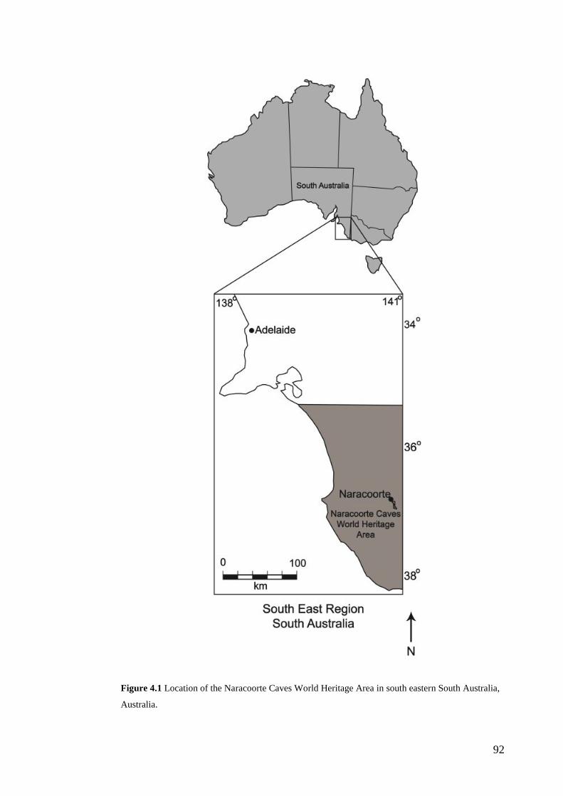
92
Figure 4.1 Location of the Naracoorte Caves World Heritage Area in south eastern South Australia,
Australia.
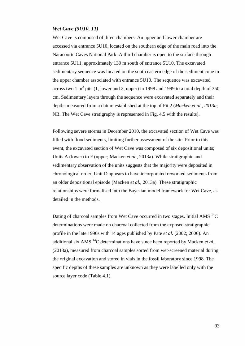
93
Wet Cave (5U10, 11) Wet Cave is composed of three chambers. An upper and lower chamber are
accessed via entrance 5U10, located on the southern edge of the main road into the
Naracoorte Caves National Park. A third chamber is open to the surface through
entrance 5U11, approximately 130 m south of entrance 5U10. The excavated
sedimentary sequence was located on the south eastern edge of the sediment cone in
the upper chamber associated with entrance 5U10. The sequence was excavated
across two 1 m2 pits (1, lower and 2, upper) in 1998 and 1999 to a total depth of 350
cm. Sedimentary layers through the sequence were excavated separately and their
depths measured from a datum established at the top of Pit 2 (Macken et al., 2013a;
NB. The Wet Cave stratigraphy is represented in Fig. 4.5 with the results).
Following severe storms in December 2010, the excavated section of Wet Cave was
filled with flood sediments, limiting further assessment of the site. Prior to this
event, the excavated section of Wet Cave was composed of six depositional units;
Units A (lower) to F (upper; Macken et al., 2013a). While stratigraphic and
sedimentary observation of the units suggests that the majority were deposited in
chronological order, Unit D appears to have incorporated reworked sediments from
an older depositional episode (Macken et al., 2013a). These stratigraphic
relationships were formalised into the Bayesian model framework for Wet Cave, as
detailed in the methods.
Dating of charcoal samples from Wet Cave occurred in two stages. Initial AMS 14C
determinations were made on charcoal collected from the exposed stratigraphic
profile in the late 1990s with 14 ages published by Pate et al. (2002; 2006). An
additional six AMS 14C determinations have since been reported by Macken et al.
(2013a), measured from charcoal samples sorted from wet-screened material during
the original excavation and stored in vials in the fossil laboratory since 1998. The
specific depths of these samples are unknown as they were labelled only with the
source layer code (Table 4.1).
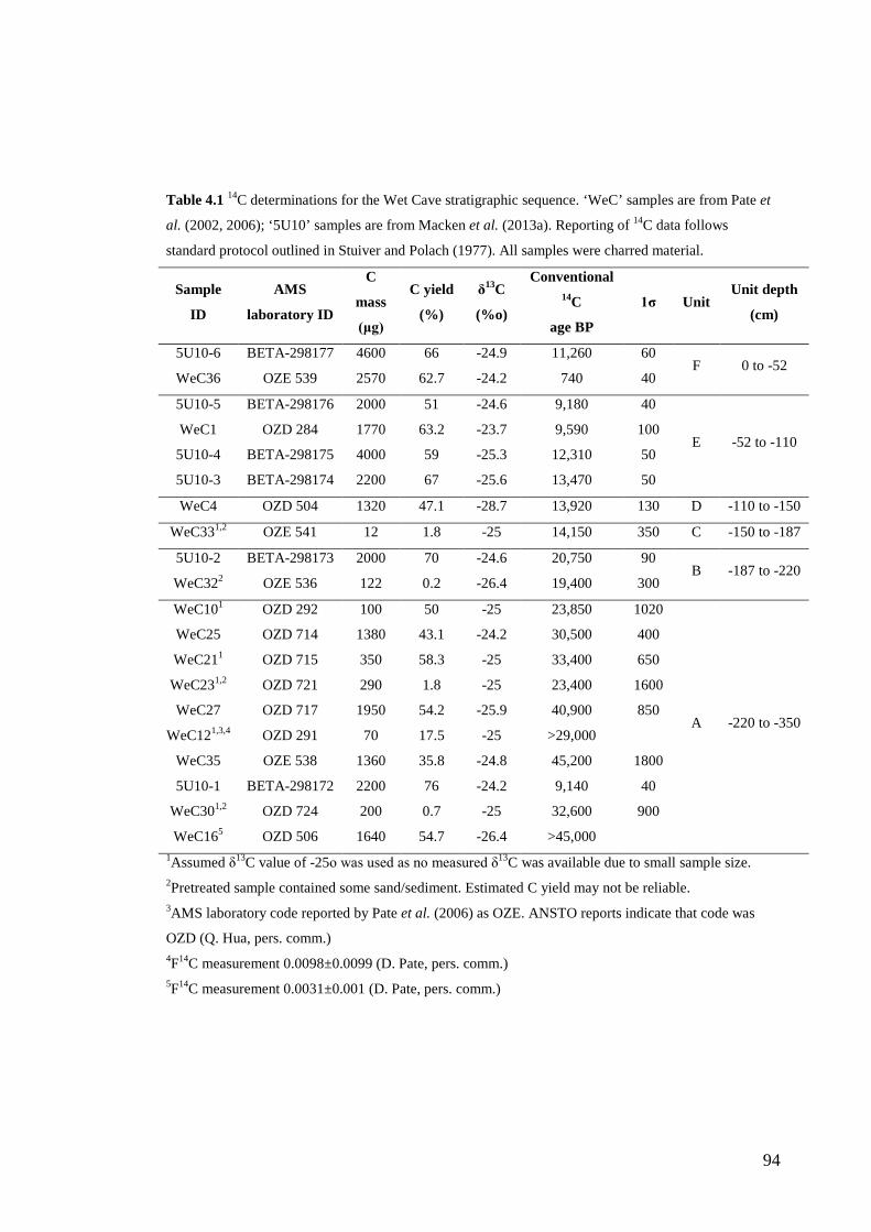
94
Table 4.1 14C determinations for the Wet Cave stratigraphic sequence. ‘WeC’ samples are from Pate et
al. (2002, 2006); ‘5U10’ samples are from Macken et al. (2013a). Reporting of 14C data follows
standard protocol outlined in Stuiver and Polach (1977). All samples were charred material.
Sample
ID
AMS
laboratory ID
C
mass
(μg)
C yield
(%)
δ13C
(%o)
Conventional 14C
age BP
1σ Unit Unit depth
(cm)
5U10-6 BETA-298177 4600 66 -24.9 11,260 60 F 0 to -52
WeC36 OZE 539 2570 62.7 -24.2 740 40
5U10-5 BETA-298176 2000 51 -24.6 9,180 40
E -52 to -110 WeC1 OZD 284 1770 63.2 -23.7 9,590 100
5U10-4 BETA-298175 4000 59 -25.3 12,310 50
5U10-3 BETA-298174 2200 67 -25.6 13,470 50
WeC4 OZD 504 1320 47.1 -28.7 13,920 130 D -110 to -150
WeC331,2 OZE 541 12 1.8 -25 14,150 350 C -150 to -187
5U10-2 BETA-298173 2000 70 -24.6 20,750 90 B -187 to -220
WeC322 OZE 536 122 0.2 -26.4 19,400 300
WeC101 OZD 292 100 50 -25 23,850 1020
A -220 to -350
WeC25 OZD 714 1380 43.1 -24.2 30,500 400
WeC211 OZD 715 350 58.3 -25 33,400 650
WeC231,2 OZD 721 290 1.8 -25 23,400 1600
WeC27 OZD 717 1950 54.2 -25.9 40,900 850
WeC121,3,4 OZD 291 70 17.5 -25 >29,000
WeC35 OZE 538 1360 35.8 -24.8 45,200 1800
5U10-1 BETA-298172 2200 76 -24.2 9,140 40
WeC301,2 OZD 724 200 0.7 -25 32,600 900
WeC165 OZD 506 1640 54.7 -26.4 >45,000 1Assumed δ13C value of -25o was used as no measured δ13C was available due to small sample size. 2Pretreated sample contained some sand/sediment. Estimated C yield may not be reliable. 3AMS laboratory code reported by Pate et al. (2006) as OZE. ANSTO reports indicate that code was
OZD (Q. Hua, pers. comm.) 4F14C measurement 0.0098±0.0099 (D. Pate, pers. comm.) 5F14C measurement 0.0031±0.001 (D. Pate, pers. comm.)
95
Blanche Cave (5U4, 5, 6) The structure of Blanche Cave and the sedimentary character, stratigraphic division
and chronology of a sediment core from the excavation site has been described by
Darrénougué et al. (2009). The Blanche Cave fossil excavation is located in the 3rd
chamber associated with entrance 5U6, approximately 400 m north west of Wet
Cave entrance 5U10. Fossil excavation in the 3rd chamber occurred between 2006
and 2007. The first excavation was conducted by Laslett (2006) who excavated four
1 m2 grid squares (A1, B1, A2 and B2) in 5 cm layers to a maximum depth of 1.1
m; however, three of the grid squares were obstructed by the presence of a large
limestone boulder. A second excavation was conducted by EHR in 2006/2007 from
two grid squares (A3 and B3), both excavated to a depth of 1 m. Excavation of
these grid squares followed the stratigraphy such that 27 individual sedimentary
layers were excavated as discrete bands, ranging from 1 to 6 cm thick (the Blanche
Cave stratigraphy is represented in Fig. 4.5, Results). The Bayesian model
developed here integrates the stratigraphic information associated with the 27
sedimentary layers described from grid squares A3 and B3, rather than the earlier,
depth-standardised spit data from Laslett (2006).
Five units (1, lower to 5, upper) have been described from the top 100 cm of the
Blanche Cave stratigraphic sequence (Darrénougué et al., 2009), corresponding to
the 27 individual sedimentary layers; however, precise depth information relating to
the units is not integrated into the Blanche age-depth model. This is because the 14C
determinations are stratigraphically constrained at a finer resolution by the 27 layers
noted from grid squares A3 and B3. A total of 40 AMS 14C determinations are
available from across the 27 layers (Darrénougué et al., 2009; St Pierre et al., 2012;
Table 4.2).
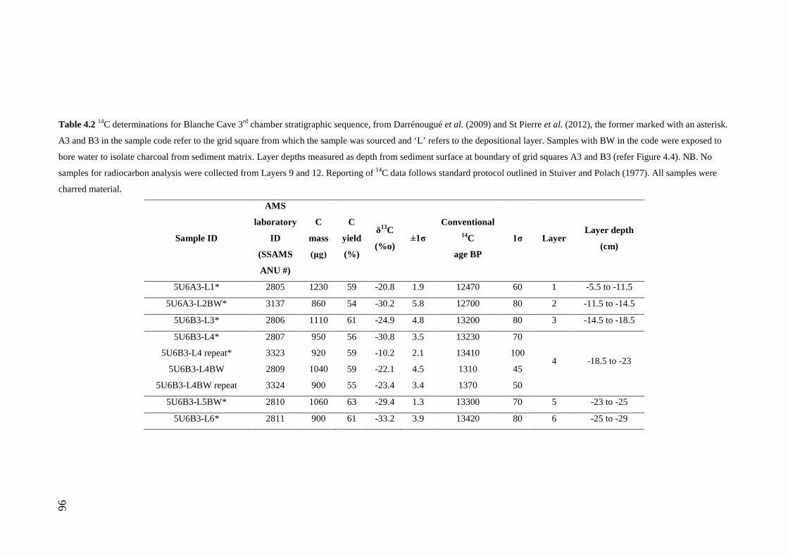
96
Table 4.2 14C determinations for Blanche Cave 3rd chamber stratigraphic sequence, from Darrénougué et al. (2009) and St Pierre et al. (2012), the former marked with an asterisk.
A3 and B3 in the sample code refer to the grid square from which the sample was sourced and ‘L’ refers to the depositional layer. Samples with BW in the code were exposed to
bore water to isolate charcoal from sediment matrix. Layer depths measured as depth from sediment surface at boundary of grid squares A3 and B3 (refer Figure 4.4). NB. No
samples for radiocarbon analysis were collected from Layers 9 and 12. Reporting of 14C data follows standard protocol outlined in Stuiver and Polach (1977). All samples were
charred material.
Sample ID
AMS
laboratory
ID
(SSAMS
ANU #)
C
mass
(μg)
C
yield
(%)
δ13C
(%o) ±1σ
Conventional 14C
age BP
1σ Layer Layer depth
(cm)
5U6A3-L1* 2805 1230 59 -20.8 1.9 12470 60 1 -5.5 to -11.5
5U6A3-L2BW* 3137 860 54 -30.2 5.8 12700 80 2 -11.5 to -14.5
5U6B3-L3* 2806 1110 61 -24.9 4.8 13200 80 3 -14.5 to -18.5
5U6B3-L4* 2807 950 56 -30.8 3.5 13230 70
4 -18.5 to -23 5U6B3-L4 repeat* 3323 920 59 -10.2 2.1 13410 100
5U6B3-L4BW 2809 1040 59 -22.1 4.5 1310 45
5U6B3-L4BW repeat 3324 900 55 -23.4 3.4 1370 50
5U6B3-L5BW* 2810 1060 63 -29.4 1.3 13300 70 5 -23 to -25
5U6B3-L6* 2811 900 61 -33.2 3.9 13420 80 6 -25 to -29
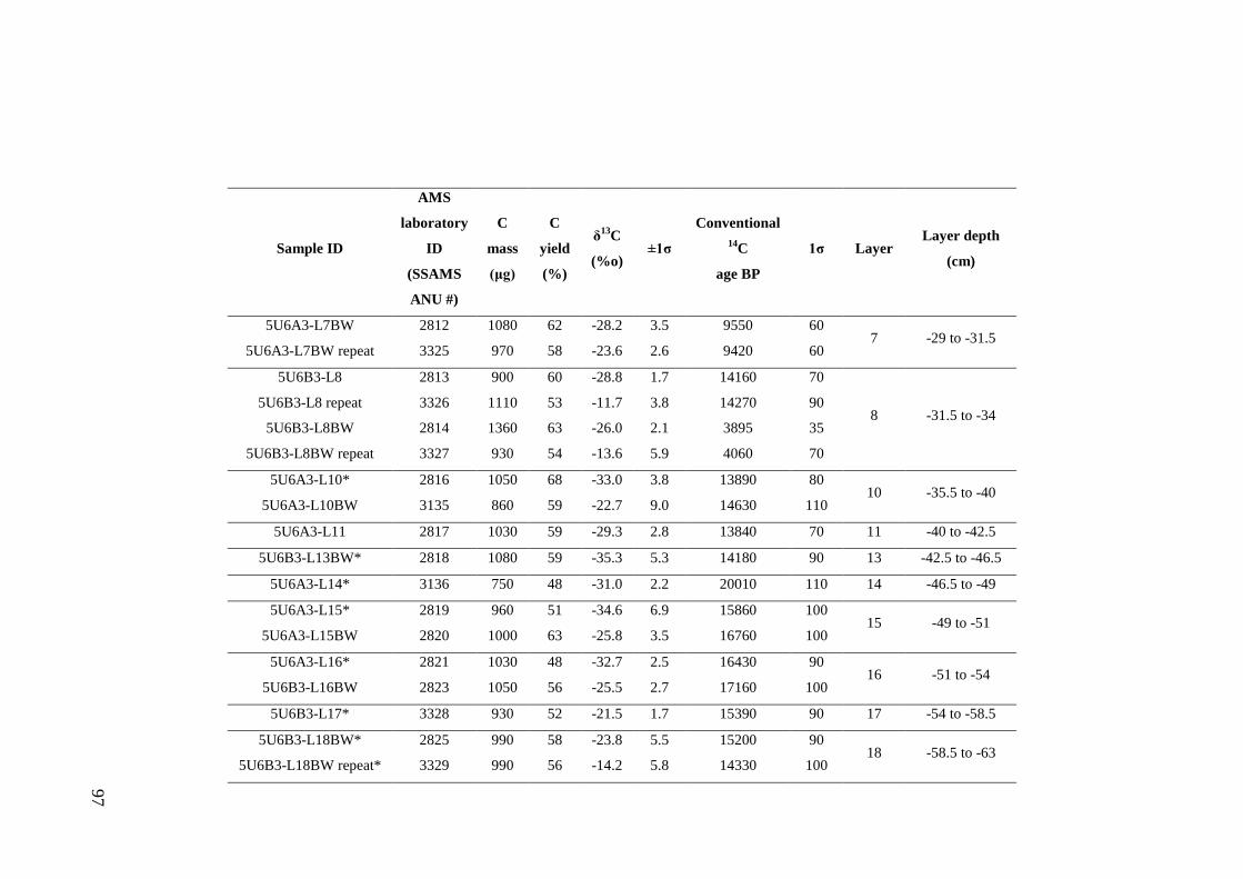
97
Sample ID
AMS
laboratory
ID
(SSAMS
ANU #)
C
mass
(μg)
C
yield
(%)
δ13C
(%o) ±1σ
Conventional 14C
age BP
1σ Layer Layer depth
(cm)
5U6A3-L7BW 2812 1080 62 -28.2 3.5 9550 60 7 -29 to -31.5
5U6A3-L7BW repeat 3325 970 58 -23.6 2.6 9420 60
5U6B3-L8 2813 900 60 -28.8 1.7 14160 70
8 -31.5 to -34 5U6B3-L8 repeat 3326 1110 53 -11.7 3.8 14270 90
5U6B3-L8BW 2814 1360 63 -26.0 2.1 3895 35
5U6B3-L8BW repeat 3327 930 54 -13.6 5.9 4060 70
5U6A3-L10* 2816 1050 68 -33.0 3.8 13890 80 10 -35.5 to -40
5U6A3-L10BW 3135 860 59 -22.7 9.0 14630 110
5U6A3-L11 2817 1030 59 -29.3 2.8 13840 70 11 -40 to -42.5
5U6B3-L13BW* 2818 1080 59 -35.3 5.3 14180 90 13 -42.5 to -46.5
5U6A3-L14* 3136 750 48 -31.0 2.2 20010 110 14 -46.5 to -49
5U6A3-L15* 2819 960 51 -34.6 6.9 15860 100 15 -49 to -51
5U6A3-L15BW 2820 1000 63 -25.8 3.5 16760 100
5U6A3-L16* 2821 1030 48 -32.7 2.5 16430 90 16 -51 to -54
5U6B3-L16BW 2823 1050 56 -25.5 2.7 17160 100
5U6B3-L17* 3328 930 52 -21.5 1.7 15390 90 17 -54 to -58.5
5U6B3-L18BW* 2825 990 58 -23.8 5.5 15200 90 18 -58.5 to -63
5U6B3-L18BW repeat* 3329 990 56 -14.2 5.8 14330 100
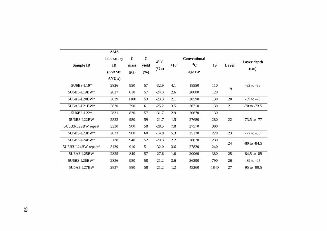
98
Sample ID
AMS
laboratory
ID
(SSAMS
ANU #)
C
mass
(μg)
C
yield
(%)
δ13C
(%o) ±1σ
Conventional 14C
age BP
1σ Layer Layer depth
(cm)
5U6B3-L19* 2826 950 57 -32.9 4.1 18550 110 19
-63 to -69
5U6B3-L19BW* 2827 810 57 -24.3 2.6 20000 120
5U6A3-L20BW* 2829 1100 53 -23.3 2.1 20590 130 20 -69 to -70
5U6A3-L21BW* 2830 790 61 -25.2 3.5 20710 130 21 -70 to -73.5
5U6B3-L22* 2831 830 57 -31.7 2.9 20670 130
22 -73.5 to -77 5U6B3-L22BW 2832 980 59 -21.7 1.5 27680 280
5U6B3-L22BW repeat 3330 900 58 -28.5 7.8 27570 300
5U6B3-L23BW* 2833 900 60 -14.8 5.3 25120 220 23 -77 to -80
5U6B3-L24BW* 3138 940 52 -29.3 2.2 28070 230 24 -80 to -84.5
5U6B3-L24BW repeat* 3139 910 51 -32.0 3.6 27820 240
5U6A3-L25BW 2835 840 57 -27.6 1.6 30060 380 25 -84.5 to -89
5U6B3-L26BW* 2836 950 58 -21.2 3.6 36290 790 26 -89 to -95
5U6A3-L27BW 2837 880 58 -21.2 1.2 43260 1840 27 -95 to -99.5
99
Materials and Methods
Bayesian age-depth models Bayesian age-depth models were developed in OxCal ver. 4.1 (Bronk Ramsey,
2008; 2009a), applying the IntCal09 calibration curve (Reimer et al., 2009), but
allowing for an offset from this for calibration in the Southern Hemisphere (SH) of
56±24 years. This offset is the same as that applied to the earliest 500 years of the
SHCal04 calibration curve (McCormac et al., 2004). Although the SH calibration
curve is only recommended back to 11,000 cal yr BP, we applied the average offset
value for the earliest 500 years of the modelled SH dataset across the entire time
period sampled in Wet and Blanche Caves. We acknowledge that the accuracy of
this offset may decline through the pre-Holocene period (ca. 11,000 to 50,000 cal yr
BP) due to a potentially more variable inter-hemispheric offset resulting from
changes in ocean circulation and carbon cycling processes under full Glacial
conditions. However, no current calibration curve is available for the SH into the
Pleistocene, necessitating the compromise approach adopted here. Leaving the
oldest ages uncalibrated, as was the approach used by Crowly (2010) would limit
the reliability with which the two sites could be correlated. Alternatively,
calibrating the pre-Holocene ages to IntCal09 (without an allowance for an inter-
hemispheric offset) would affect the reliability of any future comparison of the Wet
and Blanche Cave sequences with Northern Hemisphere data. As we apply the same
calibration offset to both sites here, the choice of calibration curve (or offset) does
not affect the correlation of the two cave sequences. Furthermore, given the
resolution of the chronological data, the offset applied does not strongly alter the
modelled chronologies for the sequences when compared with models calibrated
without an offset.
Both sites were constructed as Phases within a Sequence deposition model
(Bronk Ramsey, 2008), incorporating prior information about the order of events, as
determined from the stratigraphy. Sequence and Phase models are suitable for
sites such as caves where the rate or continuity of deposition is unknown,
contrasting with lacustrine or marine sediment profiles that might exhibit more
regular depositional phases (Bronk Ramsey, 1995; 2008). In both the Wet and
Blanche Cave sequences, few assumptions about deposition could be made from the
available stratigraphic data. For example, a possible depositional hiatus during
100
accumulation of the Wet Cave sequence is indicated by the presence of bat guano
derived materials at depth below datum (D/D) -39 to -52 cm, representing the
bottom 13 cm of Unit F; however, the duration of this event is unknown (Macken et
al., 2013a).
Boundaries were applied to the top and bottom of each sequence constraining
the maximum age of the models to 60,000 cal yr BP (conservatively earlier than the
50,000 cal yr BP limit of the IntCal09 calibration curve; Reimer et al., 2009) and
the minimum age to -50 cal yr BP (i.e., AD 2000). All modelled data are reported at
the 68.2 and 95.4% highest probability density (hpd) ranges (approximately
equivalent to 1 and 2σ uncertainty, respectively).
Wet Cave
A schematic of the OxCal model for the Wet Cave sequence is presented in Fig.
4.2a. Separate Phases were assigned to each depositional unit identified in the
Wet Cave sequence (Macken et al., 2013a). These were constrained to be in
chronological order (from Unit A, oldest, to Unit F, youngest), except for the
potentially re-worked Unit D. In order to utilise the extra chronological data
nevertheless available from Unit D (i.e., adding extra potential terminus post quem
data for the commencement of the overlying Unit E), this Phase was constrained
to lie anywhere between the start of the deposition sequence (i.e., the ‘Wet Cave
bottom’ Boundary) and the bottom of Unit E (Fig. 4.2a). In OxCal, this was
achieved by nesting the Sequence of Units A, B and C, and the independent
Phase of Unit D, within a broader Phase for Units A, B, C and D.
From stratigraphic observation it was deemed that each of the depositional units
(except Unit E) were internally heterogeneous such that no assumption of relative
chronological ordering could be made of the sediment within each of these units.
Unit E, however, demonstrated reliable sub-structure, and therefore additional sub-
Phases, themselves constrained to lie in stratigraphic order, were nested within
Unit E, representing six lenses (2:6/4, oldest, 2:6/3, 2:6/2, 2:6/1, 2:5/2, and 2:5/1,
youngest).
101
All of the 14C data for the Wet Cave samples were inserted within this model
framework as R_Dates, except WeC12 and WeC16, which were inserted with the
R_F14C function. R_F14C uses the raw F14C measurement, rather than the
calculated conventional radiocarbon age, to account for the fact that these samples
provided ‘infinite’ (‘greater than’) radiocarbon dates (Table 4.1). Outlier analysis
was applied using the ‘general’ Outlier_Model described by Bronk Ramsey
(2009b). An equal prior Outlier probability of 5% was applied to the majority of 14C determinations (R_Dates and R_F14C). However, based on the threshold
identified by Pate et al. (2006), 14C determinations from samples with extracted
carbon values of ≤100 μg C were deemed more likely to be questionable and were
given an increased prior Outlier probability of 10% (i.e., samples WeC33,
WeC23, WeC12). While Pate et al. (2006) argued that sample WeC30 had a low
extracted carbon value when compared with the other samples, its mass of 200 μg
exceeds the threshold criterion originally identified by the same authors and was
assigned a prior probability of 5% here.
Blanche Cave
A schematic of the Blanche Cave OxCal model is presented in Fig. 4.2b. The model
was constructed in a similar manner to that for Wet Cave, with separate Phases
assigned to each sedimentary layer. However, stratigraphic observations and
sedimentary data could not reliably differentiate whether Layers 23–21, 18–15, 13–
10 and 9–4 represented single, sequential depositional phases, or sediments of
mixed age within broader depositional episodes. For these sections, overlapping
sub-Phases (representing each individual layer) were nested within broader
Phases for the combined layer sections (Layers 23, 22 and 21; Layers 18, 17, 16
and 15; Layers 13, 12, 11 and 10; and Layers 09, 08, 07, 06, 05 and 04) such that no
relative ordering of the sub-Phases was presumed, a priori, within these four
broader Phases (Fig. 4.2b). The remaining layers, as well as the four broad
Phases, were then constrained to be in stratigraphic order in the overall model
Sequence (from Layer 27, oldest, to Layer 1, youngest), except for the potentially
re-worked Layer 14 (‘special event layer’ identified by Darrénougué et al., 2009).
As with Unit D in Wet Cave, the Phase for Layer 14 was constrained to lie
anywhere between the start of the deposition sequence (i.e., the ‘Blanche Cave
102
bottom’ Boundary) and the bottom of the overlying Phase (Layer 13), thus
providing additional potential terminus post quem data for the overlying strata.
The 14C data were inserted within this model framework. Outlier analysis was
again applied using the ‘general’ Outlier_Model (Bronk Ramsey, 2009b), with
a prior Outlier probability of 5% applied to all of the 14C determinations. For
this site, there was no a priori reason to believe that any of the samples were more
likely to be erroneous than others. However, six samples, 5U6B3-L8BW, 5U6B3-
L8BW repeat, 5U6A3-L7BW, 5U6A3-L7BW repeat, 5U6B3-L4BW and 5U6B3-
L4BW repeat, were so outlying that their inclusion prevented the model from
running. The prior Outlier probabilities of these samples were necessarily
increased to 100% to allow the model to run.
Temporal Duration of Phases and Potential Hiatuses between Phases
The modelled duration of Phases representing depositional units in Wet Cave and
layers or groups of layers in Blanche Cave were obtained using the Difference
query function in OxCal. Assessment of the presence and duration of potential
temporal hiatuses between successive Phases within each sequence were also
modelled using the Difference function. Difference provides the range in
calendar years between two events and can be used to test a null hypothesis (H0)
that the two events are contiguous (i.e., that, given the dating evidence available,
there is no temporal hiatus/missing sediment between the end of the first event and
the start of the next). If the calculated hpd range (for the Difference query) does
not contain 0 at a given confidence level (typically the 95.4% confidence), H0 is
rejected and there is some evidence to suggest that, at the dating resolution
available, there is missing material or a temporal gap detected between the two
events. If the null is not rejected, it is possible that the ages of the two events could
overlap. Specific cases where sedimentary observations suggest that such overlap is
possible (as a result of depositional or post-depositional mixing of materials of
different age) have been incorporated into the model priors (Wet Cave Unit D;
Blanche Cave Layer 14). All other Phases have been assumed, based on
sedimentary observations, to be successive and in stratigraphic superposition based
on age (with the exception of the individual layers within Blanche Cave Layers 9–4,
10–13, 15–18 and 23–21), and the model priors constructed accordingly.

103
Figure 4.2 Bayesian model frameworks run in OxCal for (a) Wet Cave and (b) Blanche Cave.
Phases and nested sub-Phases were constructed within Sequence models, based upon
stratigraphic and sedimentary observations of the two sites.
104
Correlation of Wet and Blanche Cave Phases The OxCal queries Order and Difference were used to examine the temporal
relationship between the Wet Cave depositional units and Blanche Cave layers.
These functions were queried for all pairwise comparisons of the posterior
probability distributions for the Wet and Blanche Cave Boundaries, which had
been saved as Priors from the output data from the two individual site models.
Order finds the probability that one event (i.e., t1) is older than another (t2).
Therefore, the function simply provides the ‘most likely’ relative ordering of events
between the two Sequences (i.e., providing a probability threshold of 50%).
Application of the Difference function provides a more rigorous, quantified
probability distribution of these relationships. As with the intra-site queries
described above, a Difference function with a 95.4% hpd range including 0
prevents rejection of the null hypothesis and implies that, given the available data,
synchrony of the two events cannot be excluded.
Results
Wet and Blanche Cave Bayesian Models Modelled ages for the upper and lower Boundaries of Wet Cave Phases are
presented in Table 4.3 and Fig. 4.3. Modelled ages for the R_Dates/R_F14Cs
and associated posterior outlier probabilities for these data are also presented in
Table 4.3. Samples 5U6-6 and 5U6-1 were both found to be 100% outliers by the
model; all other R_Dates/R_F14Cs had posterior outlier probabilities of ≤11%.
The modelled ages for the lower and upper Boundaries of Units A and F,
respectively, constrain the age of the Wet Cave sequence from 56,032–46,523 to
680– -43 cal yr BP (95.4% hpd range), ostensibly influenced by the prior maximum
and minimum age constraints applied to the model.
Modelled ages for the upper and lower Boundaries of Phases, R_Dates and
associated posterior outlier probabilities for the Blanche Cave sequence are
presented in Table 4.4. Hpd ranges of the modelled Boundaries are presented in
Fig. 4.4. While the majority of R_Dates fitted the applied model construction
well (i.e., posterior outlier probability ≤ the prior of 5%), R_Dates 5U6B3-22 and
5U6A3-L21BW returned posterior outlier probabilities of 95 and 92%, respectively.
105
Nine samples, representing R_Dates from Layers 23, 19, 18, 16, 10, 8 and 1, had
posterior outlier probability values >5%, ranging between 8 and 38%.
The modelled ages for the upper and lower-most Boundaries of the Blanche
Cave sequence (Layer 27 bottom and Layer 1 top) place the modelled Sequence
between a maximum of 59,997–46,259 cal yr BP and 14814– -50 cal yr BP, again
heavily constrained by the maximum and minimum prior ages assigned to the
model.
Phase Durations and Potential Hiatuses 68.2% and 95.4% hpd confidence ranges for the Phase durations of units and
potential hiatuses between Wet Cave units and Unit E lenses are presented in Table
4.5. Table 4.6 presents these data for the Blanche Cave layers. The duration ranges
for Wet Cave Units C, D and F and all Unit E lenses contain 0. In contrast, the
duration of Unit A ranges from 18,343 to 30,429 years. The 95.4% hpd ranges for
Units B and E also point to rejection of the null hypothesis, with upper values of
7,492, and 7,712 years respectively. All Difference functions between
successive units and Unit E lenses contain 0 at the 95.4% confidence level. As a
result, there is insufficient evidence to reject H0 (for contiguous deposition) given
the radiocarbon data available. The model prior for Unit D was such that it could
overlap in age with units A, B or C. The single 14C measurement from Unit D is
insufficient to provide refined information (compared to the unmodelled data) to
constrain this unit more precisely. For the same reason, there is insufficient
information to reject the null hypothesis that Units C and D are contiguous.
Only the duration of the Phase for Layers 18–15 of Blanche Cave does not contain
0 at the 95.4% confidence level, suggesting that, at the dating resolution available,
instantaneous deposition of each of the remaining Phases cannot be excluded.
Similarly, the null hypothesis of contiguous deposition of successive layers was not
rejected at the 95.4% confidence level for all successive layer Boundaries.
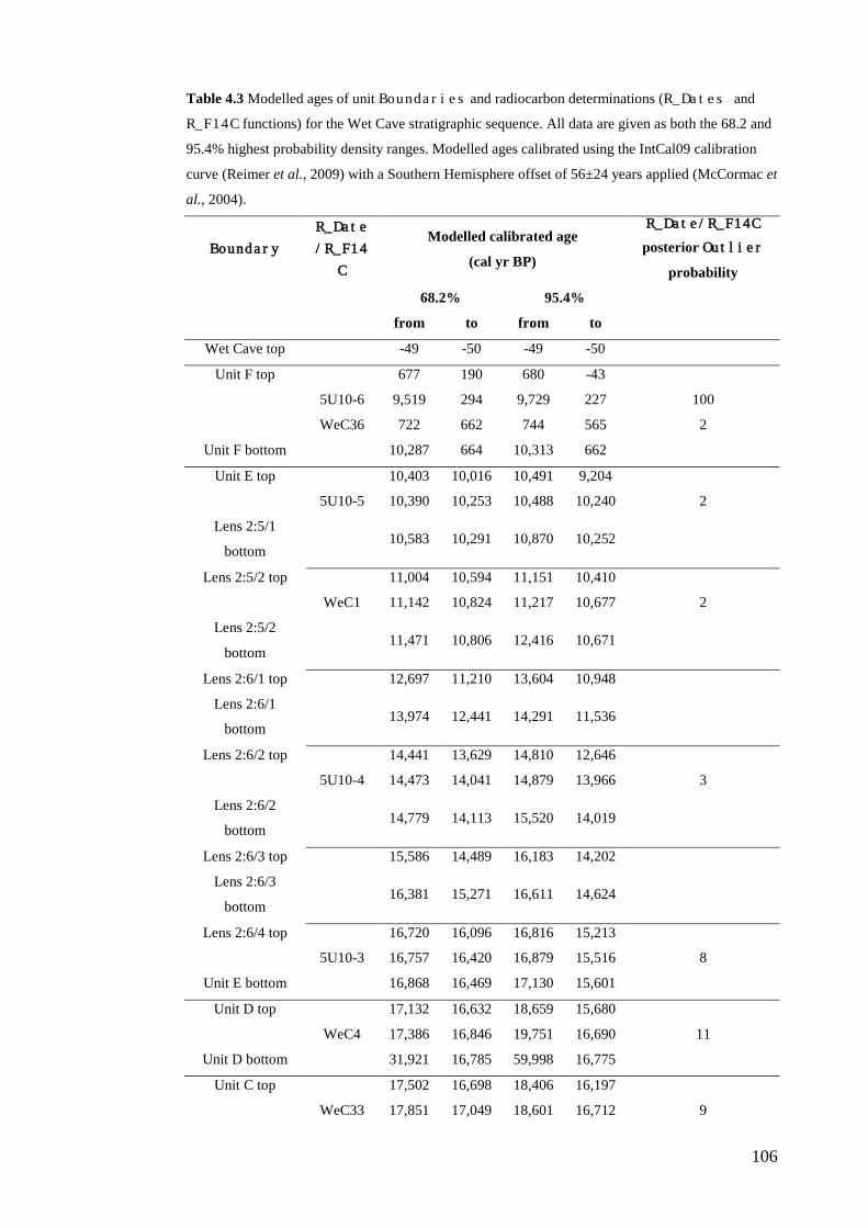
106
Table 4.3 Modelled ages of unit Boundaries and radiocarbon determinations (R_Dates and
R_F14C functions) for the Wet Cave stratigraphic sequence. All data are given as both the 68.2 and
95.4% highest probability density ranges. Modelled ages calibrated using the IntCal09 calibration
curve (Reimer et al., 2009) with a Southern Hemisphere offset of 56±24 years applied (McCormac et
al., 2004).
Boundary R_Date
/R_F14
C
Modelled calibrated age
(cal yr BP)
R_Date/R_F14C
posterior Outlier
probability
68.2% 95.4%
from to from to
Wet Cave top -49 -50 -49 -50
Unit F top 677 190 680 -43
5U10-6 9,519 294 9,729 227 100
WeC36 722 662 744 565 2
Unit F bottom 10,287 664 10,313 662
Unit E top 10,403 10,016 10,491 9,204
5U10-5 10,390 10,253 10,488 10,240 2
Lens 2:5/1
bottom 10,583 10,291 10,870 10,252
Lens 2:5/2 top 11,004 10,594 11,151 10,410
WeC1 11,142 10,824 11,217 10,677 2
Lens 2:5/2
bottom 11,471 10,806 12,416 10,671
Lens 2:6/1 top 12,697 11,210 13,604 10,948
Lens 2:6/1
bottom 13,974 12,441 14,291 11,536
Lens 2:6/2 top 14,441 13,629 14,810 12,646
5U10-4 14,473 14,041 14,879 13,966 3
Lens 2:6/2
bottom 14,779 14,113 15,520 14,019
Lens 2:6/3 top 15,586 14,489 16,183 14,202
Lens 2:6/3
bottom 16,381 15,271 16,611 14,624
Lens 2:6/4 top 16,720 16,096 16,816 15,213
5U10-3 16,757 16,420 16,879 15,516 8
Unit E bottom 16,868 16,469 17,130 15,601
Unit D top 17,132 16,632 18,659 15,680
WeC4 17,386 16,846 19,751 16,690 11
Unit D bottom 31,921 16,785 59,998 16,775
Unit C top 17,502 16,698 18,406 16,197
WeC33 17,851 17,049 18,601 16,712 9
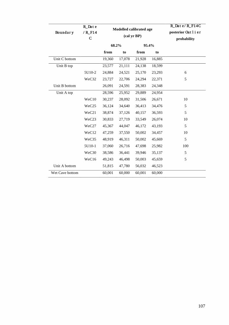
107
Boundary R_Date
/R_F14
C
Modelled calibrated age
(cal yr BP)
R_Date/R_F14C
posterior Outlier
probability
68.2% 95.4%
from to from to
Unit C bottom 19,360 17,078 21,928 16,885
Unit B top 23,577 21,111 24,138 18,599
5U10-2 24,884 24,521 25,170 23,293 6
WeC32 23,727 22,706 24,294 22,371 5
Unit B bottom 26,091 24,591 28,383 24,348
Unit A top 28,596 25,952 29,889 24,954
WeC10 30,237 28,092 31,506 26,671 10
WeC25 36,124 34,640 36,413 34,476 5
WeC21 38,874 37,126 40,157 36,593 5
WeC23 30,833 27,719 33,549 26,074 10
WeC27 45,367 44,047 46,172 43,193 5
WeC12 47,259 37,550 50,002 34,457 10
WeC35 48,919 46,311 50,002 45,669 5
5U10-1 37,060 26,716 47,698 25,982 100
WeC30 38,586 36,441 39,946 35,137 5
WeC16 49,243 46,498 50,003 45,659 5
Unit A bottom 51,815 47,780 56,032 46,523
Wet Cave bottom 60,001 60,000 60,001 60,000
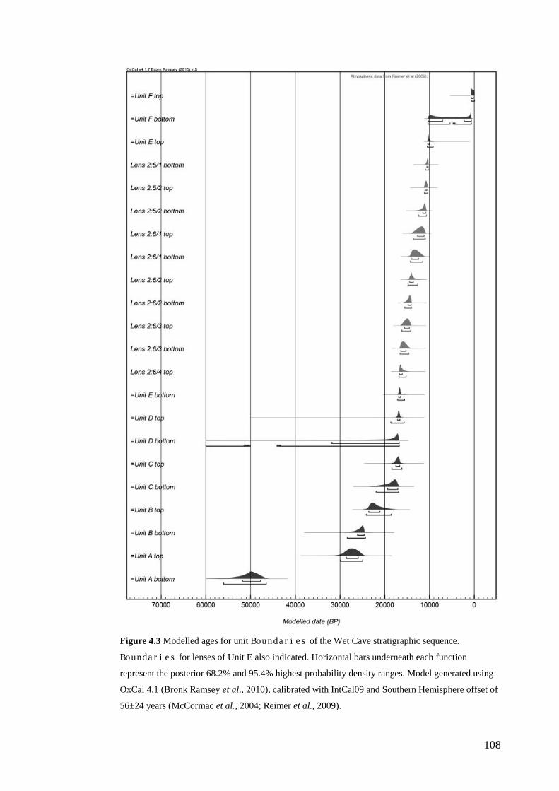
108
Figure 4.3 Modelled ages for unit Boundaries of the Wet Cave stratigraphic sequence.
Boundaries for lenses of Unit E also indicated. Horizontal bars underneath each function
represent the posterior 68.2% and 95.4% highest probability density ranges. Model generated using
OxCal 4.1 (Bronk Ramsey et al., 2010), calibrated with IntCal09 and Southern Hemisphere offset of
56±24 years (McCormac et al., 2004; Reimer et al., 2009).
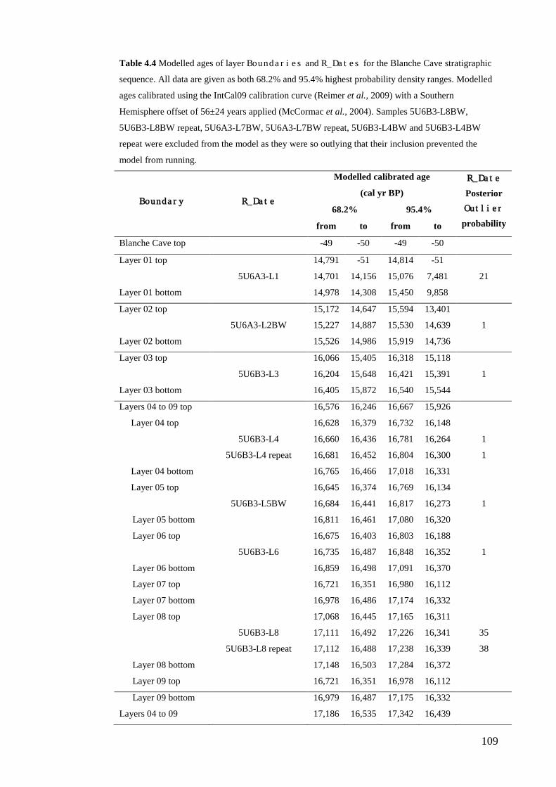
109
Table 4.4 Modelled ages of layer Boundaries and R_Dates for the Blanche Cave stratigraphic
sequence. All data are given as both 68.2% and 95.4% highest probability density ranges. Modelled
ages calibrated using the IntCal09 calibration curve (Reimer et al., 2009) with a Southern
Hemisphere offset of 56±24 years applied (McCormac et al., 2004). Samples 5U6B3-L8BW,
5U6B3-L8BW repeat, 5U6A3-L7BW, 5U6A3-L7BW repeat, 5U6B3-L4BW and 5U6B3-L4BW
repeat were excluded from the model as they were so outlying that their inclusion prevented the
model from running.
Boundary R_Date
Modelled calibrated age
(cal yr BP) R_Date
Posterior Outlier
probability 68.2% 95.4%
from to from to
Blanche Cave top -49 -50 -49 -50
Layer 01 top 14,791 -51 14,814 -51
5U6A3-L1 14,701 14,156 15,076 7,481 21
Layer 01 bottom 14,978 14,308 15,450 9,858
Layer 02 top 15,172 14,647 15,594 13,401
5U6A3-L2BW 15,227 14,887 15,530 14,639 1
Layer 02 bottom 15,526 14,986 15,919 14,736
Layer 03 top 16,066 15,405 16,318 15,118
5U6B3-L3 16,204 15,648 16,421 15,391 1
Layer 03 bottom 16,405 15,872 16,540 15,544
Layers 04 to 09 top 16,576 16,246 16,667 15,926
Layer 04 top 16,628 16,379 16,732 16,148
5U6B3-L4 16,660 16,436 16,781 16,264 1
5U6B3-L4 repeat 16,681 16,452 16,804 16,300 1
Layer 04 bottom 16,765 16,466 17,018 16,331
Layer 05 top 16,645 16,374 16,769 16,134
5U6B3-L5BW 16,684 16,441 16,817 16,273 1
Layer 05 bottom 16,811 16,461 17,080 16,320
Layer 06 top 16,675 16,403 16,803 16,188
5U6B3-L6 16,735 16,487 16,848 16,352 1
Layer 06 bottom 16,859 16,498 17,091 16,370
Layer 07 top 16,721 16,351 16,980 16,112
Layer 07 bottom 16,978 16,486 17,174 16,332
Layer 08 top 17,068 16,445 17,165 16,311
5U6B3-L8 17,111 16,492 17,226 16,341 35
5U6B3-L8 repeat 17,112 16,488 17,238 16,339 38
Layer 08 bottom 17,148 16,503 17,284 16,372
Layer 09 top 16,721 16,351 16,978 16,112
Layer 09 bottom 16,979 16,487 17,175 16,332
Layers 04 to 09 17,186 16,535 17,342 16,439
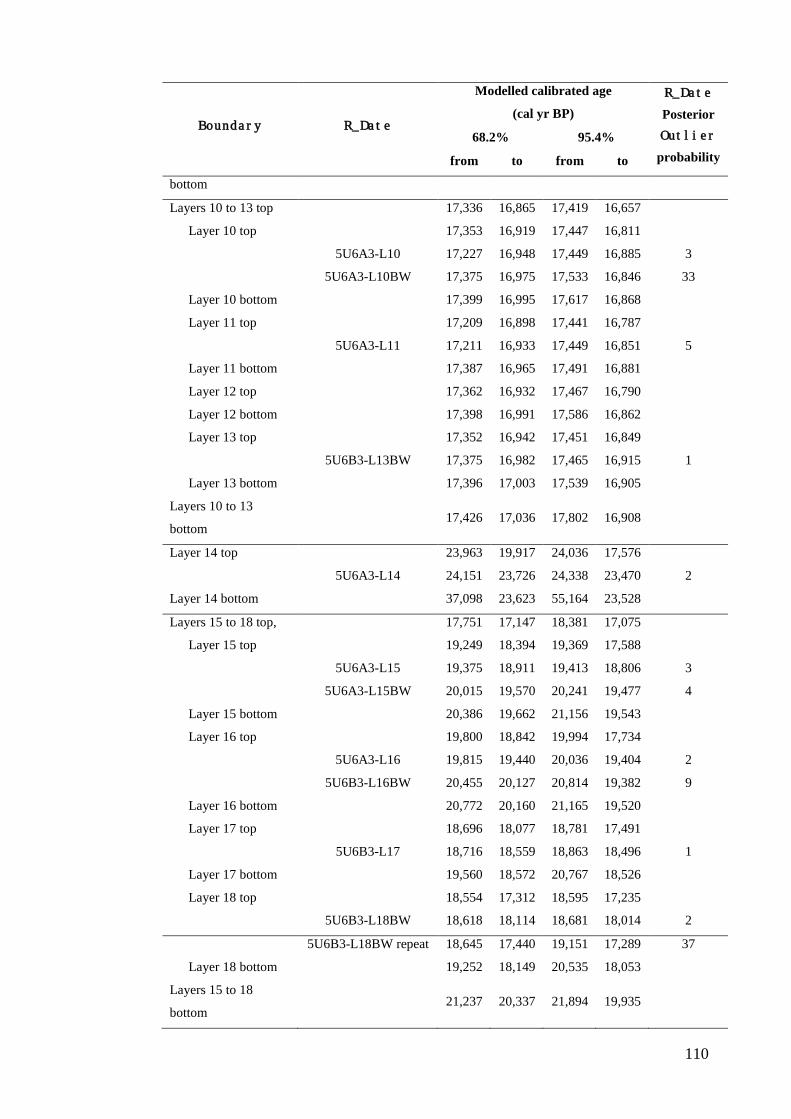
110
Boundary R_Date
Modelled calibrated age
(cal yr BP) R_Date
Posterior Outlier
probability 68.2% 95.4%
from to from to
bottom
Layers 10 to 13 top 17,336 16,865 17,419 16,657
Layer 10 top 17,353 16,919 17,447 16,811
5U6A3-L10 17,227 16,948 17,449 16,885 3
5U6A3-L10BW 17,375 16,975 17,533 16,846 33
Layer 10 bottom 17,399 16,995 17,617 16,868
Layer 11 top 17,209 16,898 17,441 16,787
5U6A3-L11 17,211 16,933 17,449 16,851 5
Layer 11 bottom 17,387 16,965 17,491 16,881
Layer 12 top 17,362 16,932 17,467 16,790
Layer 12 bottom 17,398 16,991 17,586 16,862
Layer 13 top 17,352 16,942 17,451 16,849
5U6B3-L13BW 17,375 16,982 17,465 16,915 1
Layer 13 bottom 17,396 17,003 17,539 16,905
Layers 10 to 13
bottom 17,426 17,036 17,802 16,908
Layer 14 top 23,963 19,917 24,036 17,576
5U6A3-L14 24,151 23,726 24,338 23,470 2
Layer 14 bottom 37,098 23,623 55,164 23,528
Layers 15 to 18 top, 17,751 17,147 18,381 17,075
Layer 15 top 19,249 18,394 19,369 17,588
5U6A3-L15 19,375 18,911 19,413 18,806 3
5U6A3-L15BW 20,015 19,570 20,241 19,477 4
Layer 15 bottom 20,386 19,662 21,156 19,543
Layer 16 top 19,800 18,842 19,994 17,734
5U6A3-L16 19,815 19,440 20,036 19,404 2
5U6B3-L16BW 20,455 20,127 20,814 19,382 9
Layer 16 bottom 20,772 20,160 21,165 19,520
Layer 17 top 18,696 18,077 18,781 17,491
5U6B3-L17 18,716 18,559 18,863 18,496 1
Layer 17 bottom 19,560 18,572 20,767 18,526
Layer 18 top 18,554 17,312 18,595 17,235
5U6B3-L18BW 18,618 18,114 18,681 18,014 2
5U6B3-L18BW repeat 18,645 17,440 19,151 17,289 37
Layer 18 bottom 19,252 18,149 20,535 18,053
Layers 15 to 18
bottom 21,237 20,337 21,894 19,935
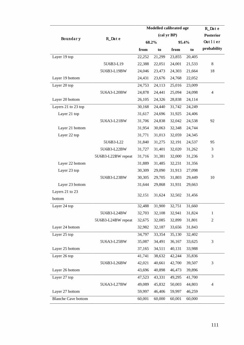
111
Boundary R_Date
Modelled calibrated age
(cal yr BP) R_Date
Posterior Outlier
probability 68.2% 95.4%
from to from to
Layer 19 top 22,252 21,299 23,855 20,405
5U6B3-L19 22,388 22,051 24,001 21,533 8
5U6B3-L19BW 24,046 23,473 24,303 21,664 18
Layer 19 bottom 24,431 23,676 24,768 22,052
Layer 20 top 24,753 24,113 25,016 23,009
5U6A3-L20BW 24,878 24,441 25,094 24,098 4
Layer 20 bottom 26,105 24,326 28,838 24,114
Layers 21 to 23 top 30,168 24,440 31,742 24,249
Layer 21 top 31,617 24,696 31,925 24,406
5U6A3-L21BW 31,706 24,838 32,042 24,538 92
Layer 21 bottom 31,954 30,063 32,348 24,744
Layer 22 top 31,771 31,013 32,059 24,345
5U6B3-L22 31,840 31,275 32,191 24,537 95
5U6B3-L22BW 31,727 31,401 32,020 31,262 3
5U6B3-L22BW repeat 31,716 31,381 32,000 31,236 3
Layer 22 bottom 31,889 31,485 32,231 31,356
Layer 23 top 30,309 29,090 31,913 27,098
5U6B3-L23BW 30,305 29,705 31,803 29,449 10
Layer 23 bottom 31,644 29,868 31,931 29,663
Layers 21 to 23
bottom 32,151 31,624 32,502 31,456
Layer 24 top 32,488 31,900 32,751 31,660
5U6B3-L24BW 32,703 32,108 32,941 31,824 1
5U6B3-L24BW repeat 32,675 32,085 32,899 31,801 2
Layer 24 bottom 32,982 32,187 33,656 31,843
Layer 25 top 34,797 33,354 35,130 32,402
5U6A3-L25BW 35,087 34,491 36,167 33,625 3
Layer 25 bottom 37,165 34,511 40,131 33,988
Layer 26 top 41,741 38,632 42,244 35,836
5U6B3-L26BW 42,021 40,661 42,700 39,507 3
Layer 26 bottom 43,696 40,898 46,473 39,896
Layer 27 top 47,523 43,331 49,295 41,700
5U6A3-L27BW 49,089 45,832 50,003 44,803 4
Layer 27 bottom 59,997 46,406 59,997 46,259
Blanche Cave bottom 60,001 60,000 60,001 60,000
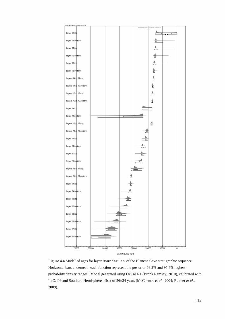
112
Figure 4.4 Modelled ages for layer Boundaries of the Blanche Cave stratigraphic sequence.
Horizontal bars underneath each function represent the posterior 68.2% and 95.4% highest
probability density ranges. Model generated using OxCal 4.1 (Bronk Ramsey, 2010), calibrated with
IntCal09 and Southern Hemisphere offset of 56±24 years (McCormac et al., 2004; Reimer et al.,
2009).
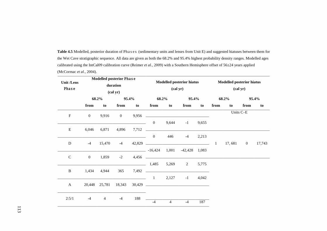
113
Table 4.5 Modelled, posterior duration of Phases (sedimentary units and lenses from Unit E) and suggested hiatuses between them for
the Wet Cave stratigraphic sequence. All data are given as both the 68.2% and 95.4% highest probability density ranges. Modelled ages
calibrated using the IntCal09 calibration curve (Reimer et al., 2009) with a Southern Hemisphere offset of 56±24 years applied
(McCormac et al., 2004).
Unit /Lens Phase
Modelled posterior Phase
duration
(cal yr)
Modelled posterior hiatus
(cal yr)
Modelled posterior hiatus
(cal yr)
68.2% 95.4% 68.2% 95.4% 68.2% 95.4%
from to from to from to from to from to from to
F 0 9,916 0 9,956 Units C–E
0 9,644 -1 9,655
E 6,046 6,871 4,896 7,712
0 446 -4 2,213
1 17, 681 0 17,743 D -4 15,470 -4 42,829
-16,424 1,001 -42,428 1,083
C 0 1,859 -2 4,456
1,485 5,269 2 5,775
B 1,434 4,944 365 7,492
1 2,127 -1 4,042
A 20,448 25,781 18,343 30,429
2:5/1 -4 4 -4 188
-4 4 -4 187
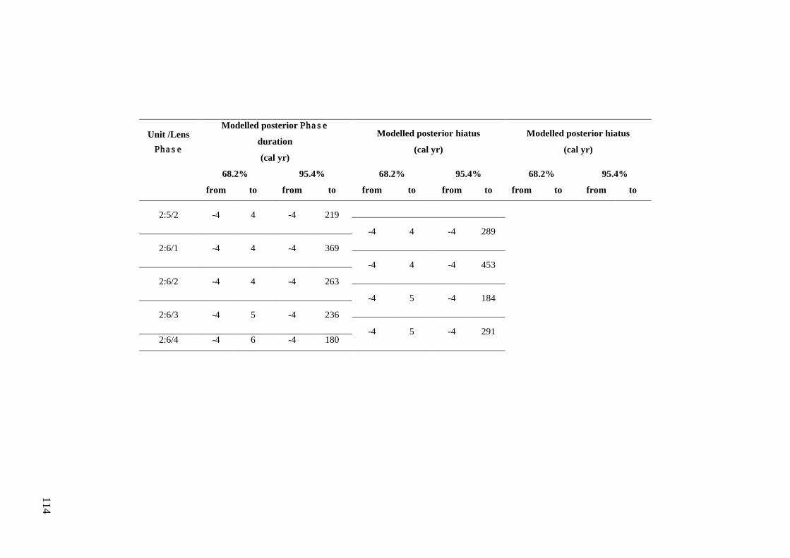
114
Unit /Lens Phase
Modelled posterior Phase
duration
(cal yr)
Modelled posterior hiatus
(cal yr)
Modelled posterior hiatus
(cal yr)
68.2% 95.4% 68.2% 95.4% 68.2% 95.4%
from to from to from to from to from to from to
2:5/2 -4 4 -4 219
-4 4 -4 289
2:6/1 -4 4 -4 369
-4 4 -4 453
2:6/2 -4 4 -4 263
-4 5 -4 184
2:6/3 -4 5 -4 236
-4 5 -4 291
2:6/4 -4 6 -4 180
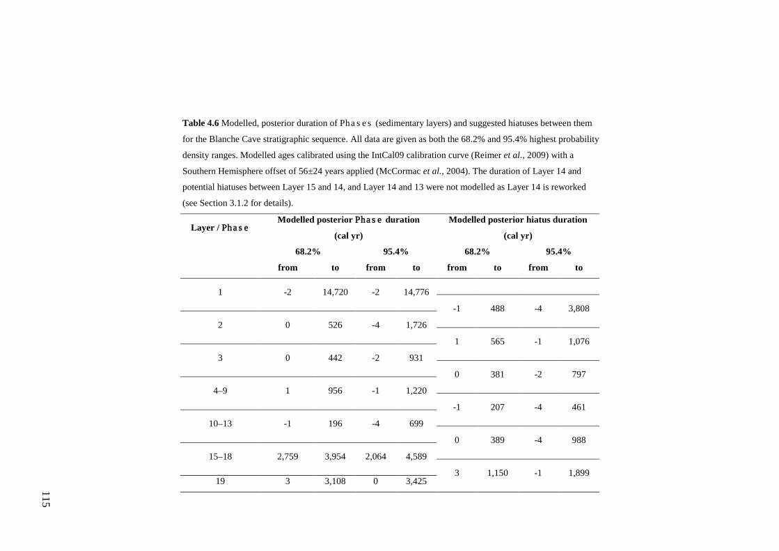
115
Table 4.6 Modelled, posterior duration of Phases (sedimentary layers) and suggested hiatuses between them
for the Blanche Cave stratigraphic sequence. All data are given as both the 68.2% and 95.4% highest probability
density ranges. Modelled ages calibrated using the IntCal09 calibration curve (Reimer et al., 2009) with a
Southern Hemisphere offset of 56±24 years applied (McCormac et al., 2004). The duration of Layer 14 and
potential hiatuses between Layer 15 and 14, and Layer 14 and 13 were not modelled as Layer 14 is reworked
(see Section 3.1.2 for details).
Layer / Phase Modelled posterior Phase duration
(cal yr)
Modelled posterior hiatus duration
(cal yr)
68.2% 95.4% 68.2% 95.4%
from to from to from to from to
1 -2 14,720 -2 14,776
-1 488 -4 3,808
2 0 526 -4 1,726
1 565 -1 1,076
3 0 442 -2 931
0 381 -2 797
4–9 1 956 -1 1,220
-1 207 -4 461
10–13 -1 196 -4 699
0 389 -4 988
15–18 2,759 3,954 2,064 4,589
3 1,150 -1 1,899 19 3 3,108 0 3,425
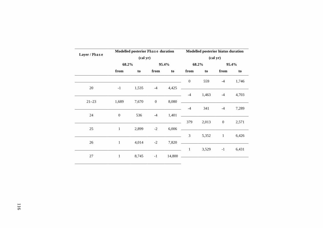
116
Layer / Phase Modelled posterior Phase duration
(cal yr)
Modelled posterior hiatus duration
(cal yr)
68.2% 95.4% 68.2% 95.4%
from to from to from to from to
0 559 -4 1,746
20 -1 1,535 -4 4,425
-4 1,463 -4 4,703
21–23 1,689 7,670 0 8,080
-4 341 -4 7,289
24 0 536 -4 1,401
379 2,013 0 2,571
25 1 2,899 -2 6,006
3 5,352 1 6,426
26 1 4,014 -2 7,820
1 3,529 -1 6,431
27 1 8,745 -1 14,800
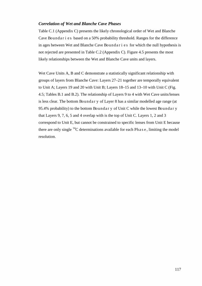
117
Correlation of Wet and Blanche Cave Phases Table C.1 (Appendix C) presents the likely chronological order of Wet and Blanche
Cave Boundaries based on a 50% probability threshold. Ranges for the difference
in ages between Wet and Blanche Cave Boundaries for which the null hypothesis is
not rejected are presented in Table C.2 (Appendix C). Figure 4.5 presents the most
likely relationships between the Wet and Blanche Cave units and layers.
Wet Cave Units A, B and C demonstrate a statistically significant relationship with
groups of layers from Blanche Cave: Layers 27–21 together are temporally equivalent
to Unit A; Layers 19 and 20 with Unit B; Layers 18–15 and 13–10 with Unit C (Fig.
4.5; Tables B.1 and B.2). The relationship of Layers 9 to 4 with Wet Cave units/lenses
is less clear. The bottom Boundary of Layer 8 has a similar modelled age range (at
95.4% probability) to the bottom Boundary of Unit C while the lowest Boundary
that Layers 9, 7, 6, 5 and 4 overlap with is the top of Unit C. Layers 1, 2 and 3
correspond to Unit E, but cannot be constrained to specific lenses from Unit E because
there are only single 14C determinations available for each Phase, limiting the model
resolution.
118
Figure 4.5 Correlation of Wet Cave units and Blanche Cave layers based on 50% probability threshold
for relative order of Boundaries and null Difference distributions (i.e., where there is no
difference in the modelled age of Boundaries between the two sites). Black dotted lines indicate
relationship between Wet Cave units with groups of Blanche Cave layers. * represents an inferred
correlation between Layers 1, 2 and 3 with Wet Cave lenses, based on the balance of probabilities,
stratigraphic information and un-modelled 14C determinations. Gaps in the stratigraphic sequences
indicate position of Unit D (Wet Cave) and Layer 14 (Blanche Cave), both of which contain material of
mixed age and origin. Groups of layers in Blanche Cave that were modelled as single Phases are
indicated by the grey lines between stratigraphic layers.
119
Discussion
Wet and Blanche Cave Bayesian age-depth model priors The aggraded sedimentary sequences in Wet and Blanche Caves reflect multiple
modes of accumulation and source materials through the late Pleistocene to Holocene
period, incorporating the last glacial cycle. Sedimentary characteristics range from
aeolian and water transported red-brown sandy clays in Units A and Layers 27 to 21,
to aeolian derived pale brown to yellow sands, intersected by likely water transported
narrow lenses of darker, silty sands through Units B to E and Layers 20 to 2 (Macken
et al., 2013a). While the sequence of sediment types in Wet and Blanche Caves is
similar, the depth profiles of analogous layers between the sites vary. The thicker
depositional strata of Wet Cave contrast with the narrower and more discrete layers of
Blanche Cave. As discussed in Macken et al. (2013a) these differences in the depth
profiles of the two deposits likely result from local accumulation and post-depositional
processes associated with each cave and depositional site, despite their geographic
proximity (ca. 400 m).
As discussed by Bronk Ramsey (2008), depositional processes that should be
considered when developing priors for Bayesian age models include (i) the
mechanisms underlying deposition, (ii) random events and (iii) abrupt changes in
deposition mode. Deposition of sediments into caves is controlled by a range of
interacting factors including cave entrance type, prevailing climatic conditions,
proximal vegetation cover and local sediments and their transport (e.g., Farrand, 2001;
Hearty et al., 2004; White, 2007). These factors are expected to have affected the
mechanisms of sediment deposition into Wet and Blanche Caves, primarily aeolian
(dust) and water transportation (Darrénougué et al. 2009; Macken et al., 2013a).
Random events such as sedimentary slumping and transport of flood-sediments also
shape stratigraphic sequences in caves (e.g., Kos, 2001) and have been observed in the
Naracoorte Caves in modern times (e.g., filling of Wet Cave with flood sediments and
surficial sediment washes and pooling water in Blanche Cave, following severe storms
in December 2010). Stratigraphic features such as cut and fills, lenses and flame
structures indicate that these random processes have influenced the two cave sequences
during their accumulation through the last ca. 60,000 cal yrs. Abrupt changes in
deposition are reflected by well-defined sedimentary transitions in both cave sequences
(e.g., Unit A to B in Wet Cave), contrasting with other interfaces that are less clear and
120
may reflect more gradual changes in sediment source and/or depositional mode (e.g.,
Layers 9 to 4 in Blanche Cave).
We suggest that the Sequence depositional model in OxCal, incorporating Phases
of uniform prior duration is of particular utility when working with complex
depositional environments, such as caves, as they are based on fewer assumptions
about the rate and process of deposition when compared with other OxCal deposition
models (e.g., P_Sequence) and that they are also suitable when modelling sequences
for which there are few radiocarbon determinations relative to the timespan covered by
the study site. By constructing the Wet and Blanche Cave Bayesian age-depth models
within a Sequence framework, the order of the 14C data within depositional
units/layers could be integrated a priori based on an inference of stratigraphic
superposition, such that deeper sediments were deposited earlier than those higher in
the profile. The finest stratigraphic resolution that could be applied to the Wet Cave
model was the depositional units, with the exception of Unit E for which the six lenses
were well defined (Fig. 4.5). In contrast, the potential temporal resolution available in
Blanche Cave was much finer, with 27 individual sedimentary layers that could be
integrated as prior stratigraphic divisions within the model.
In two cases (Wet Cave Unit D and Blanche Cave Layer 14) the assumption of
stratigraphic superposition was challenged by sedimentary data and/or observations,
resulting in more complex model constructions but, nonetheless, could be accounted
for using a series of nested Phases. The OxCal Phase function also allowed us to
differentiate prior information for which we had varying levels of certainty, as was the
case for the depositional and temporal relationships of groups of individual layers in
Blanche Cave (e.g., Layers 9 to 4), particularly where sedimentary transitions were
less clear. We note that these layer groupings in the Blanche Cave model contrast with
the depositional units defined for Blanche Cave by Darrénougué et al. (2009). These
differences arise because the priors for the Blanche Cave model were informed by
observations directly from the exposed, excavated section from which the radiocarbon
samples were collected. In addition, not all layers were evident in the stratigraphic core
from which the units were defined (St Pierre et al., 2012).
121
Outliers Wet Cave R_Dates 5U10-1 and 5U10-6 were identified as 100% outliers and were
thus excluded by OxCal in the model output. As noted by Bronk Ramsey et al. (2010),
there are four main circumstances under which 14C data may conflict with each other
or with model priors. These are: (i) uncertainty in the reservoir 14C concentration, (ii)
sample contamination, (iii) incorrect 14C measurement and (iv) uncertainties in the
chronological models applied. In applying an offset to the calibration for the SH, we
have tried to account for systematic uncertainties associated with scenario (i). While
the offset we have applied might not be wholly accurate for the entire calibration
range, at the chronological resolution available for Wet and Blanche Caves, the impact
of this is expected to be negligible. Scenarios (ii) and (iii) may be sample-specific and
result in individual or consistent offsets and biases among the 14C measurements.
These scenarios would be indistinguishable from each other based on the 14C data
alone. Scenario (iv) accounts for circumstances where sample(s) may be residual
(older than context) or intrusive (younger than context) (Bronk Ramsey et al., 2010).
Uncertainties may also arise when parameters of a deposition model are not clearly
defined (e.g., k, the number of accumulation events per unit depth for use in
P_Sequence models). Such a scenario is not expected to apply to the less rigid
Sequence models applied to Wet and Blanche Caves, unless the assignment of
sequential Phases or overlapping sub-Phases is incorrect.
Sample 5U10-1 may be an outlier because of measurement issues (scenario iii);
however, it is not possible to confirm which of the circumstances identified above
most likely accounts for its far outlying 14C determination in comparison to the other
samples from Unit A. Sample 5U10-1 was previously noted as being wrongly
associated with Unit A (Macken et al., 2013a), consistent with scenario (iv) above.
However, rather than representing re-worked material as a result of post-depositional
mixing of younger sediments with the Pleistocene sediments of Unit A, it was
hypothesised that the charcoal sample was disturbed by human activity, most likely
during excavation when the deeper sections of the profile were exposed. The consistent
character of the sediments from Unit A and Pleistocene ages for all other samples
supports this hypothesis and argues against contamination of this section of the
sequence with younger material, an important consideration for subsequence analysis
of the fauna preserved in Unit A.
122
The rejection of sample 5U10-6 points to OxCal accepting the young Holocene age for
Unit F given the model prior. The age constraint for the Wet Cave upper Boundary
of AD 2000 strongly influences the modelled age for the upper Boundary of Unit F
and likely contributes to the rejection of 5U10-6 which does not conform to this
Boundary and is older than some samples from Unit E. In contrast to Unit A, for
which little contamination is evident, it is more difficult to determine the extent of
potential mixing of Pleistocene aged material into Unit F. The presence of European
artifacts (glass and ceramic shards) in Unit F informed the assumption that materials,
including charcoal, may have been deposited into Wet Cave in more modern times and
also suggests that anthropogenic disturbance of the upper sections of the Wet Cave
profile may have occurred (Macken et al., 2013a). Based on these assumptions, sample
5U10-6 is expected to reflect contamination of Unit F with Pleistocene aged sediments,
possibly by transport and mixing of sediments of different ages at the top of the
sequence by human activity. In this case, rejection of sample 5U10-6 by OxCal is
assumed to be consistent with scenario (iv) and points to post-depositional mixing of
material of different ages in Unit F.
Blanche Cave samples 5U6A3-L21BW and 5U6B3-L22 were identified as outliers by
OxCal and were heavily down-weighted in the model. The identification of these
samples as outliers seemed somewhat unexpected compared to our prior expectation of
the data (based upon casual ‘eyeballing’). As a sensitivity test of the whole model, an
alternative Blanche Cave model was run with R_Dates from Layers 23 to 21
grouped together into a single Phase but without allocating them to individual sub-
Phases. In this latter case, samples 5U6A3-L21BW and 5U6B3-L22 were no longer
identified as outliers.
Unless otherwise specified in the model prior, a uniform Phase prior is assumed in
OxCal. Within this prior, there is no bias towards longer or shorter Phases and it is
assumed that all of the events within the group are equally likely to occur anywhere
between the start and end of the Phase; that is, there is no internal sorting (Bronk
Ramsey, 2009a). Of the three R_Dates from Layer 22, the unmodelled, calibrated
age of sample 5U6B3-L22 is ca. 7,000 cal yr younger than the other two samples.
Under the uniform Phase prior, if the true duration of the Layer 22 sub-Phase was
represented by the R_Dates, then the 14C determinations would be expected to be
123
more evenly spread out (i.e., it would be extremely unlikely, though not impossible, to
have two closely temporally spaced dates, with a third dating so much younger). On
this basis the model found 5U6B3-L22 to be an outlier. Of the scenarios previously
discussed, the reason for such an outlier could be because of either (ii), (iii) or (iv). As
noted, in the alternative model in which all of the 14C determinations from Layers 23 to
21 are assessed together under a uniform Phase prior (rather than constrained within
individual sub-Phases), sample 5U6B3-L22 is not found to be an outlier because it is
supported by the similarity in age with sample 5U6A3-L21. Despite this, we did not
use the alternative model as it provided no capacity to gain additional precision or
resolution available from the individual layers within the broader Phases, if they
were found to be chronologically independent within the model. However, as samples
5U6A3-L21BW and 5U6B3-L22 were found to be outliers within the more complex
final model adopted, no greater resolution was gained by assessing these layers
individually. We suggest that the most likely reason for this is that the samples are
intrusive (i.e., younger than the context), limiting the resolution at which the layers
within the broader Phase of Layer 23–21 can be evaluated.
Posterior outlier probabilities of 18 to 38% for samples from Layers 8, 10, 18 and 19
suggests that the likelihoods do not fit the model prior particularly well. That said,
despite the elevated outlier probabilities of these samples compared to the initial 5%
prior probabilities applied, there is still a greater probability of the samples not being,
rather than of their being, outliers as all posterior probabilities are < 50%. Using the
Outlier_Model, OxCal downweights the impact of these samples on the model
output.
In contrast, 14C determinations for samples 5U6B3-L17 and 5U6B3-L18BW were
discarded by Darrénougué et al. (2009) who considered that they had infiltrated the
stratigraphic section, presumably during sample collection. However, the posterior
outlier probabilities for these samples in the model do not support this assertion. If the
model prior for Blanche Cave had been set such that Layer 19 is older than (>) Layer
18 > Layer 17 > Layer 16, then it is highly likely that samples 5U6B3-L17 and
5U6B3-L18BW would have been identified as outliers. However, the model prior
grouped Layers 18 to 15 within a single Phase highlighting that whether or not
124
samples are identified as outliers clearly depends on the specifics of the model prior
applied.
Holocene 14C determinations from Blanche Cave Layers 4, 7 and 8 were excluded
from the model as, even with the Outlier_Model applied, the model would not run
with these samples included. Despite their exclusion from the model, the Holocene
aged samples are expected to represent post-depositional reworking of younger
material through the sedimentary section (St Pierre et al., 2012). This inference is
supported by a U-series age of 4.72±0.21 ka from a soda straw stalactite collected from
nearby grid square A1 at a depth of 20–25 cm, corresponding to Layers 3 and 4 in grid
squares A3 and B3 (St Pierre et al., 2012; Fig. 4.5). Further, it is less likely that the
Holocene 14C determinations are incorrect due to measurement error or disturbance
during collection as in each of Layers 4, 7 and 8, two samples provide very similar
ages that are younger than the 14C determinations of adjacent samples.
Additional Holocene aged soda straw stalactites were measured from depths 0–5 cm,
5–10 cm and 55–60 cm from grid squares A1 and B2, corresponding to Layers 1, and
17 and 18 in grid squares A3 and B3 respectively (St Pierre et al., 2012). As noted by
St Pierre et al. (2012), reworking may have occurred during or following deposition as
a result of material worked down through cracks in the sediment during dry Phases
or worked down as a result of trampling by animals or humans. However, it is more
difficult to explain why many of the 14C and soda straw U-series ages are relatively
well ordered such that age increases with depth (St Pierre et al., 2012). The
sedimentary layers described from grid squares A3 and B3 are moderately intact;
flame structures present in Layers 4 and 8 and a laterally constrained channel fill from
Layer 1 through to Layer 7 in grid square B3 provide some evidence of physical
disturbance (Fig. 4.5). However, given the limited lateral extent of these structures, it
is unlikely that these features represent significant, broad scale turnover or reworking
of sedimentary material through the profile. Despite this, as multiple and varied
chronological samples returned Holocene ages for the upper section of the deposit
through Layer 8, we caution interpretations of the vertebrate fossil material from these
sections which, being small, may have moved through the sedimentary layers in a
similar way to the charcoal and soda straws. In contrast, we suggest that the Holocene-
aged straw measured from grid square A1 at 55–60 cm depth may not reflect
125
contamination of Layers 17 and 18 in grid squares A3 and B3; the 14C data from these
layers accord well with the adjacent samples within the combined Phase of Layers
18–15 with none rejected as outliers.
Phase durations, hiatuses and chronological interpretation As a result of the relatively small number of 14C data available relative to the long
temporal coverage of the two sites, the precision of the unit and layer Boundaries is
on the order of 100s to 1000s of years. If there were more radiocarbon data, the
modelled Boundaries would be expected to be more precise and, in turn, allow for
more precise estimates of the durations of individual units and layers and potential
hiatuses between them. This would also allow for a more robust comparison of the
temporal correlation of the two sites. However, despite the overall low precision of the
modelled Boundary ages, statistical estimates of the minimum and maximum age of
individual depositional Phases would otherwise have been unavailable from the
unmodelled 14C determinations.
The modelled Phase durations for Wet Cave reveal slow and rapid phases of
accumulation through the depositional sequence. Unit A represents the longest phase
between both Wet and Blanche Caves, followed by Units E and B. In the case of Units
C, D and F, the null hypothesis of instantaneous accumulation (or, at least, deposition
from <1 calendar year) cannot be rejected on the basis of the dating evidence available.
For Unit C, this results from having only a single radiocarbon measurement from this
Unit. The same is true for Unit F, where the identification of sample 5U10-6 as an
outlier (100% posterior Outlier probability) gave only a single ‘reliable’
radiocarbon determination. It is expected that, were additional radiocarbon (or other
chronological) data available, these units would not, in reality, represent instantaneous
deposition. The presence of silty laminations through the sands of Unit C supports this
assumption, as such banding or horizonation is rarely associated with sediments that
have slumped or been deposited during a single event, as observed in the homogenous
sands of nearby Robertson Cave (Forbes et al., 2007). Sandy laminations observed in
Unit F also argue against instantaneous deposition for the upper-most section of Wet
Cave.
126
Having only a single radiocarbon measurement for Unit D accounts for the inability of
the model to discount the null hypothesis of instantaneous deposition for this Phase,
as noted for Units C and F. However, the mottled orange and brown, poorly sorted
sandy clays of Unit D do not contain internal structuring as observed in the former two
units. The sedimentary character of Unit D and presence of megafaunal bone material
suggests that it contains sediments of similar type, origin and age as Unit A (Macken et
al., 2013a). An hypothesis for the presence of Unit D at the top of Pit 1,
stratigraphically above Unit C, is that it represents late Pleistocene aged materials from
another part of the cave, transported and slumped down the sedimentary cone during
accumulation of the Wet Cave sequence. If this were the case, then it may represent an
anomalous, single ‘instantaneous’ event that re-worked sedimentary and fossil material
of mixed origin and age.
In Blanche Cave, only a single Phase (Layers 18–15) returned a modelled duration
statistically indistinguishable from 0 years at the 95.4% confidence level. Limited
rejection of the null hypothesis for the majority of Blanche Cave Phases again
results from the small number of radiocarbon measurements for many layers.
However, the sedimentary and stratigraphic character of some layers suggests that they
may represent single, ‘instantaneous’ depositional episodes associated with surficial
water movement of sediments during single flood events (e.g., Layers 7, 9 and 20). For
these layers, rejection of the null is in accord with the inference of rapid deposition
based on sedimentary observations.
The coarse resolution of the modelled Boundaries for both the Wet and Blanche
Cave sequences similarly limits the capacity of the model to detect temporal gaps in
accumulation between successive Phases and/or where there may be missing
material between the end of one Phase and the start of the next. In all cases, the null
hypothesis for contiguous deposition was not able to be rejected at the 95.4%
confidence level. A hiatus of 1,485 to 5,269 cal yrs between Units B and C and of 379
to 2,013 cal years between layers 25 and 24 was measured at the 68.2% confidence
level. As these hiatuses are not supported at the higher confidence level, there is little
that can be concluded from these values; however, as both Wet and Blanche Caves
have large open-roof window entrances, it is unlikely that prolonged hiatuses in
deposition into the caves occurred due to the constant movement and flux of dust
127
across the landscape. The potential for post-depositional erosion of sediments from
these sites is more difficult to ascertain.
In contrast, breaks in deposition have been argued for two late Pleistocene cave
sequences from south eastern Australia; the inner chamber of Robertson Cave located
ca. 6 km south of Wet Cave and McEachern’s Deathtrap Cave, ca. 100 km south of the
Naracoorte Caves World Heritage Area. The sedimentary sequences from both of these
caves reflect hiatuses in deposition over the peak of the last glacial cycle, the Last
Glacial Maximum (LGM; Kos, 2001; Forbes et al., 2007). McEachern’s Deathtrap
Cave has a narrow-pipe entrance that became blocked with sands during the LGM,
contrasting with the larger roof-window entrances of Wet and Blanche Caves that are
not expected to become blocked in this way. Although Robertson Cave has a roof-
window style entrance, the inner chamber is expected to have blocked as a result of
high sediment loads in the entrance chamber, which restricted movement through
narrower caverns in the cave system connecting the two chambers. In McEachern’s
Deathtrap Cave there is also evidence for the post-depositional erosion of sediments as
a result of groundwater fluctuations, resulting in a gap in the record.
A potential hiatus in deposition between Units E and F of Wet Cave was indicated by
the presence of bat guano derived materials at the transition between these units,
reflecting minimal sediment input prior to the deposition of the dark brown silty sands
of Unit F (Forbes and Bestland, 2006; Macken et al., 2013a). The presence of a
flowstone at the transitional boundary of Units E and F was also noted in the original
excavation notes for Wet Cave; however, it is unknown if the flowstone was attached
to the cave wall or free floating, limiting the extent to which it confirms a hiatus in
sediment deposition at the end of the Pleistocene in Wet Cave. There is no other
sedimentary or stratigraphic evidence to indicate temporal breaks and/or the loss of
sediments through erosion in Wet Cave, nor in Blanche Cave. However, we suggest
that the lack of statistically significant evidence for depositional breaks detected
through the sequences is more likely a consequence of the dating resolution, rather
than implicit evidence for continuous deposition into Wet and Blanche Caves during
the last glacial cycle. Ultimately, more 14C determinations or other dating evidence is
required to improve the resolution of the modelled Boundaries and hence, detection
128
of potential hiatuses that may be of shorter duration than the resolution of the current
chronology.
Correlation of Wet and Blanche Cave Phases As discussed by Blaauw et al. (2007), demonstrating synchronicity of events is
dependent upon the assumed duration of the events of interest. In the case of Wet and
Blanche Caves, the events are depositional episodes that are expected to represent,
through sedimentary and stratigraphic characteristics, prevailing climatic conditions.
Thus, transitions between events represented by stratigraphic boundaries are assumed
to ultimately reflect changes in a range of interacting and complex climatic and
depositional parameters operating at both a local and regional scale (Forbes and
Bestland, 2007; Forbes et al., 2007; Macken et al., 2013a). In most cases, the Blanche
Cave layers were expected to be of shorter duration than the Wet Cave units as the
latter represent individual phases that together may be consolidated into longer
depositional periods (units) characterised by (a) similar sediment type and depositional
mode and (2) relatively constant prevailing climatic conditions during their deposition.
Relationships between the Wet and Blanche Cave Phases support this assumption as
each Wet Cave unit is temporally equivalent to multiple Blanche Cave layers (Fig.
4.5).
On the balance of probabilities, Blanche Cave Layers 27 to 21 together overlap in age
with Wet Cave Unit A as reflected in the order of the associated Boundaries and
the statistically indistinguishable posterior calibrated hpd ranges of Unit A top and
Layer 21 bottom. Layers 27 to 21 in Blanche Cave therefore represent sub-divisions of
the pre-LGM period which may be used to assess the fossil assemblage at a finer
resolution, contrasting with the longer time-averaged fauna (i.e., the number of years
an assemblage took to accumulate; Hadly, 1999) represented in Unit A as a whole and
combined Layers 27 to 21.
Blanche Cave Layers 19 and 20, 18–15 and 13–10 similarly provide a reliable, finer
resolution for the LGM period represented in Wet Cave Units B and C, respectively.
Modelled ages for the start and end of deposition of Layers 19 and 20 are both
statistically indistinguishable from the start and end of the deposition of Unit B;
however, given the relative stratigraphic positions of Layers 19 and 20, they are
129
expected to provide successive sub-divisions of the first LGM period. A similar pattern
is noted for the modelled ages of the start and end of the deposition of combined
Layers 18–15 and 13–10 with Unit C but nonetheless, provide two sub-divisions of the
second LGM period represented in the deposits. The statistical correlation of multiple
Boundaries between Wet and Blanche Cave arises as a result of the resolution of
the model, limiting its ability to temporally differentiate the upper and lower
Boundaries of Phases, similar to the impacts noted for the durations and hiatuses.
For Layers 9–4, there is insufficient information to reject the possibility that they
temporally overlap both Units B and/or C of Wet Cave. As these layers contain
Holocene aged material, the temporal relationship of Layers 9–4 with Wet Cave is not
meaningful. In addition, these layers are considered to be unsuitable for inclusion in
the analyses of the small mammal faunas unless it can be shown that no fossil material
has intruded into this section of the Blanche Cave stratigraphy.
The relationships between Blanche Cave Layers 1 to 3 with Wet Cave are not well
differentiated at the available resolution of the modelled Sequences. Order
suggests that Layer 3 is temporally constrained between the bottom Boundary of
Unit E and the bottom Boundary of Lens 2:5/2. The upper Boundary of Layer 1 is
statistically indistinguishable from all Wet Cave Boundaries from 2:6/3 top to Unit
F top, a consequence of the insufficient resolution of the modelled data to identify a
more precise relationship. As noted in the results, the modelled age for the upper
Boundary of Layer 1 is strongly influenced by the prior applied for the top of the
Blanche Cave sequence of AD 2000. While this model prior was appropriate for
constraining the minimum age of the sequence (based on disturbance through human
access to the site in modern times and the presence of Pinus pollen indicating
European settlement; Darrénougué et al., 2009), it is unlikely to be the true minimum
age for fossil material contained within Layer 1. As there was only one radiocarbon
determination available for Layer 1, the true age of this Phase is not well represented
by the model. While the correlation is consistent with the output of the model,
knowledge of the two sites suggests that Layer 1 is more likely to be temporally
equivalent to Lenses 2:6/4 to 2:6/2 and cautions inferences that may be drawn from the
fossil material of Layer 1 when compared with Wet Cave.
130
Conclusion Bayesian age-depth models were developed for the fossil-bearing sedimentary
sequences of Wet and Blanche Caves in south eastern South Australia, utilising
available 14C determinations and stratigraphic information. At the dating resolution
available from these data, the modelled ages for the start and end of successive units
and layers within the two sites show that deposition was contiguous and characterised
by phases of slower and more rapid accumulation, as is common for many cave
deposits. Statistically supported temporal correlation of depositional phases between
Wet and Blanche Caves provides a robust basis for comparative analysis of the fossil
assemblages contained within them, and builds upon previous stratigraphic
correlations that were based only on sparse, individually calibrated radiocarbon data
and sedimentary descriptions.
In contrast to other age-depth models available in OxCal, Sequence was applied for
modelling Wet and Blanche Caves where only the relative order of events within the
two sites could be incorporated as a model prior. By incorporating the depositional
events as Phases within the model, we were also able to incorporate uncertainties
associated with the internal continuity of individual layers and units. Phases also
offered flexibility in the model where there was more uncertainty associated with both
(a) the stratigraphic relationships of individual layers in Blanche Cave and (b) known
reworked layers which nevertheless provided extra terminus post quem data for
overlying layers.
Despite the rigour applied to the chronologies of Wet and Blanche Caves, the
resolution of the models is limited by the few 14C determinations relative to the late
Pleistocene to Holocene time-span covered by the sites. However, while we
acknowledge that the resolution of the model would be improved if more 14C
determination were available, we also recognise the practical limitations in obtaining
large numbers of radiocarbon data in palaeontological studies. These include the
availability of research funds and samples suitable for dating, as well as limitations
presented by the time resolution captured in study sites. In light of these challenges, we
recommend that, where possible more than one sample is obtained from each
stratigraphic layer. Nonetheless, analysis of radiocarbon data within a Bayesian
framework provides a means of critically evaluating site chronologies, regardless of

131
the number of 14C determinations available, and provides a means of quantifying the
uncertainties associated with the start and end of different accumulation phases.
Acknowledgements We thank Drs Quan Hua, Donald Pate and Stewart Fallon for providing additional 14C
data associated with Wet and Blanche Caves. EHR acknowledges major funding for
the current Naracoorte research via the Federal Government Caring for Our Country
grant OC11-00487.
132
5. Late Quaternary small mammal faunas of the
Naracoorte Caves World Heritage Area
Citation Macken, A.C. and Reed, E.H. (2013) Late Quaternary small mammal faunas of the
Naracoorte Caves World Heritage Area. Transactions of the Royal Society of South
Australia 137, 53–67.
Contribution of Authors Amy Macken:
• Devised and planned the project.
• Identified and registered the specimens from Wet, Robertson and Blanche
Cave used for the research presented in the manuscript.
• Prepared manuscript for publication.
Elizabeth Reed:
• Excavated fossil material from Robertson Cave Entrance Chamber and
Blanche Cave used in the research.
• Provided funding for the project.
• Provided comments on the manuscript and advice on revisions.
Signed .................................................................................. Date ............................
Amy Macken
School of Biological Sciences, Flinders University
Signed ................................................................................. Date ............................
Elizabeth Reed
School of Biological Sciences, Flinders University
133
Abstract The vertebrate fossil deposits of the Naracoorte Caves in south eastern South
Australia preserve a long-term record of local faunas. We provide here an updated
list of small mammal faunas of late Quaternary (c. <50 ka) aged fossil assemblages
from Wet, Robertson and Blanche Caves as a basis for understanding past and
future patterns in species occurrence. The updated list includes seven species
previously unrecorded from the <50 ka period from this region. Of these, two
species (Dasycercus sp. indet. and Pseudomys novaehollandiae) are new to the
Naracoorte fossil record and have no known regional historical (European
colonisation to 1950) or contemporary (post 1950) distribution. Review of fossil
collections such as these is crucial for providing up-to-date species occurrence data
which can be used to establish baselines of past species diversity and information
about the past geographic ranges of individual taxa through time.
Introduction The vertebrate fossil deposits of the Naracoorte Caves World Heritage Area
(NCWHA) contain a record of faunal diversity for the south east region of South
Australia spanning the Middle Pleistocene to Holocene (Reed and Bourne, 2000,
2009). Research into the Naracoorte Cave fossil assemblages has made significant
contributions to knowledge of (i) Middle to Late Pleistocene faunal communities of
southern Australia (e.g., Prideaux et al., 2007; Macken et al., 2012), (ii) taxonomy
and systematics of extinct and living faunas (e.g., Prideaux and Wells, 1998;
Williams, 1999; Prideaux, 2004), (iii) vertebrate taphonomy of cave deposits (e.g.,
Reed, 2006, 2009) and (iv) environmental change over the Pleistocene (e.g., Forbes
and Bestland, 2007, Darrénougué et al., 2009, Macken et al. 2013a). As the
Naracoorte Caves contain ‘megafauna’ species such as Thylacoleo carnifex,
Zygomaturus trilobus, ‘Procoptodon’ gilli and Wonambi naracoortensis, research
into the cave assemblages has provided insights into the diversity, distribution and
extinction dynamics of this group of large body-sized faunas at the end of the
Pleistocene (e.g., Pate et al., 2006; Prideaux et al., 2007).
The Naracoorte Caves also contain extensive assemblages of smaller body-sized
taxa, providing a reference for the diversity, distribution and historical extinction
dynamics of these often understudied faunas through the late Quaternary (e.g.,
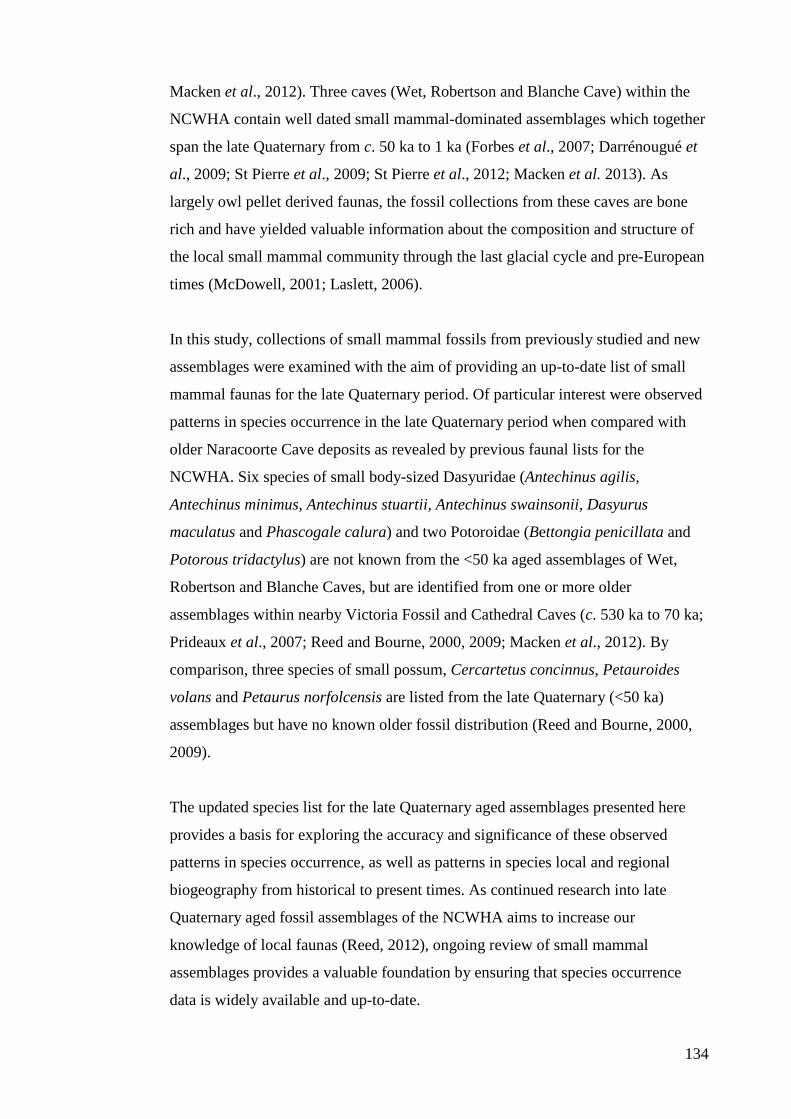
134
Macken et al., 2012). Three caves (Wet, Robertson and Blanche Cave) within the
NCWHA contain well dated small mammal-dominated assemblages which together
span the late Quaternary from c. 50 ka to 1 ka (Forbes et al., 2007; Darrénougué et
al., 2009; St Pierre et al., 2009; St Pierre et al., 2012; Macken et al. 2013). As
largely owl pellet derived faunas, the fossil collections from these caves are bone
rich and have yielded valuable information about the composition and structure of
the local small mammal community through the last glacial cycle and pre-European
times (McDowell, 2001; Laslett, 2006).
In this study, collections of small mammal fossils from previously studied and new
assemblages were examined with the aim of providing an up-to-date list of small
mammal faunas for the late Quaternary period. Of particular interest were observed
patterns in species occurrence in the late Quaternary period when compared with
older Naracoorte Cave deposits as revealed by previous faunal lists for the
NCWHA. Six species of small body-sized Dasyuridae (Antechinus agilis,
Antechinus minimus, Antechinus stuartii, Antechinus swainsonii, Dasyurus
maculatus and Phascogale calura) and two Potoroidae (Bettongia penicillata and
Potorous tridactylus) are not known from the <50 ka aged assemblages of Wet,
Robertson and Blanche Caves, but are identified from one or more older
assemblages within nearby Victoria Fossil and Cathedral Caves (c. 530 ka to 70 ka;
Prideaux et al., 2007; Reed and Bourne, 2000, 2009; Macken et al., 2012). By
comparison, three species of small possum, Cercartetus concinnus, Petauroides
volans and Petaurus norfolcensis are listed from the late Quaternary (<50 ka)
assemblages but have no known older fossil distribution (Reed and Bourne, 2000,
2009).
The updated species list for the late Quaternary aged assemblages presented here
provides a basis for exploring the accuracy and significance of these observed
patterns in species occurrence, as well as patterns in species local and regional
biogeography from historical to present times. As continued research into late
Quaternary aged fossil assemblages of the NCWHA aims to increase our
knowledge of local faunas (Reed, 2012), ongoing review of small mammal
assemblages provides a valuable foundation by ensuring that species occurrence
data is widely available and up-to-date.
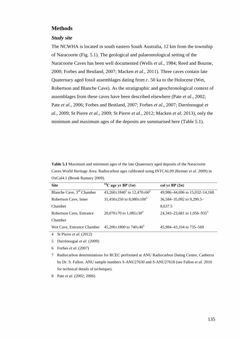
135
Methods
Study site The NCWHA is located in south eastern South Australia, 12 km from the township
of Naracoorte (Fig. 5.1). The geological and palaeontological setting of the
Naracoorte Caves has been well documented (Wells et al., 1984; Reed and Bourne,
2000; Forbes and Bestland, 2007; Macken et al., 2011). Three caves contain late
Quaternary aged fossil assemblages dating from c. 50 ka to the Holocene (Wet,
Robertson and Blanche Cave). As the stratigraphic and geochronological context of
assemblages from these caves have been described elsewhere (Pate et al., 2002;
Pate et al., 2006; Forbes and Bestland, 2007; Forbes et al., 2007; Darrénougué et
al., 2009; St Pierre et al., 2009; St Pierre et al., 2012; Macken et al. 2013), only the
minimum and maximum ages of the deposits are summarised here (Table 5.1).
Table 5.1 Maximum and minimum ages of the late Quaternary aged deposits of the Naracoorte
Caves World Heritage Area. Radiocarbon ages calibrated using INTCAL09 (Reimer et al. 2009) in
OxCal4.1 (Bronk Ramsey 2009).
Site 14C age yr BP (1σ) cal yr BP (2σ)
Blanche Cave, 3rd Chamber 43,260±18401 to 12,470±602 49,986–44,696 to 15,032–14,168
Robertson Cave, Inner
Chamber
31,450±250 to 8,080±1003 36,584–35,092 to 9,290.5–
8,637.5
Robertson Cave, Entrance
Chamber
20,070±70 to 1,085±304 24,343–23,681 to 1,056–9353
Wet Cave, Entrance Chamber 45,200±1800 to 740±405 45,984–43,334 to 735–569
4 St Pierre et al. (2012)
5 Darrénougué et al. (2009)
6 Forbes et al. (2007)
7 Radiocarbon determinations for RCEC performed at ANU Radiocarbon Dating Centre, Canberra
by Dr. S. Fallon. ANU sample numbers S-ANU27630 and S-ANU27618 (see Fallon et al. 2010
for technical details of technique).
8 Pate et al. (2002; 2006)
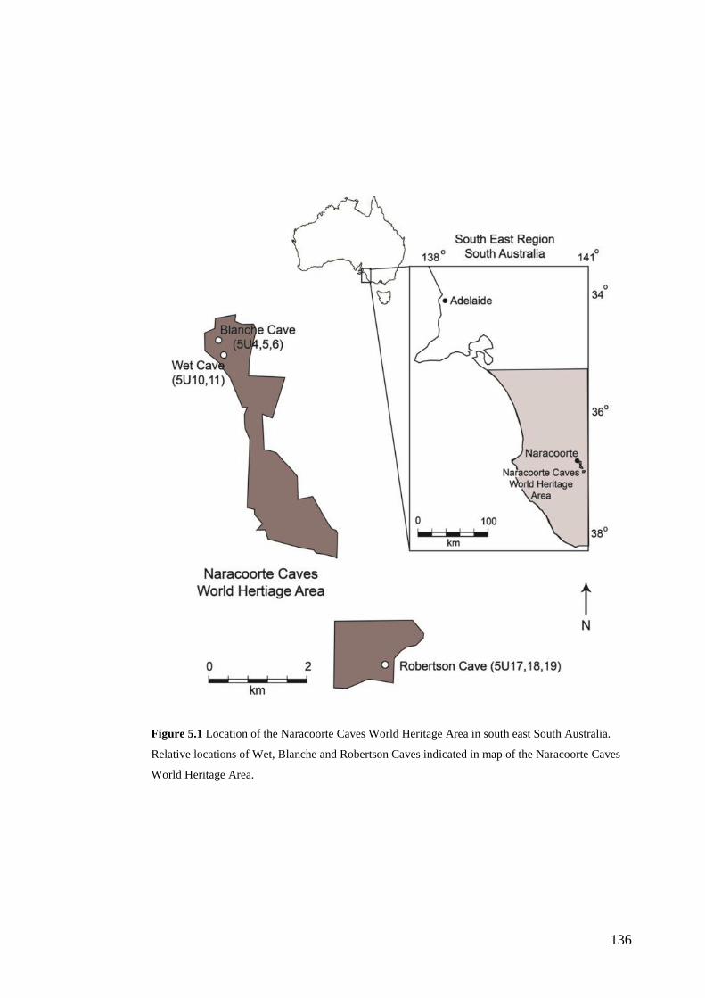
136
Figure 5.1 Location of the Naracoorte Caves World Heritage Area in south east South Australia.
Relative locations of Wet, Blanche and Robertson Caves indicated in map of the Naracoorte Caves
World Heritage Area.
137
Fossil assemblages Wet Cave (5U10, 11)
A late Quaternary aged sedimentary and fossil sequence within the entrance
chamber (5U10) of Wet Cave was first studied by McDowell (2001), following
excavation of the site in 1997 and 1998. The sequence was excavated according to
sedimentary layers across two separate 1 m2 pits, identified as Pit 1 (lower) and Pit
2 (upper) to a combined depth of 3.5 m. Each pit was divided into four 0.5 m2
quadrants (A–D), which were excavated separately (McDowell, 2001). A review of
the stratigraphy and chronology for the Wet Cave deposit is compiled in Macken et
al. (2013a).
McDowell (2001) analysed a total of 17,214 cranial specimens from Wet Cave, the
largest single fossil sample identified and analysed from the NCWHA. Marsupial
specimens from all four quadrants were re-examined in the current study. Muridae
specimens composed 81% of the assemblage analysed by McDowell (2001). Due to
this volume of material, only a sub-sample of Muridae specimens from the
assemblage was re-examined in the present study. In layers where the total murid
number of identified specimens (NISP) was <300 as documented in McDowell
(2001), material from all quadrants (A–D) was re-examined. For layers where the
total NISP was >300, only specimens from a single quadrant were assessed. In most
cases, sub-samples were examined from quadrant A with the exception of layer
1:7/3 where the sub-sample was derived from quadrant C. Previously unsorted and
unidentified specimens from this collection were also identified.
Only those specimens re-examined from the Wet Cave assemblage are discussed
here. The studied specimens were registered to the Flinders University
Palaeontology Register (FU20000–20997) and are stored in the Palaeontology
Laboratory on site in the NCWHA.
Robertson Cave (5U17, 18, 19) Two sites within Robertson Cave contain late Quaternary aged faunal assemblages.
The Robertson Cave Inner Chamber (RCIC) fossil assemblage was excavated and
analysed by McDowell (2001). Due to the similar taxonomic composition of the
138
RCIC to other late Quaternary aged assemblages of the NCWHA, only specimens
of species unique to this deposit were re-examined.
Fossil material was excavated by EHR from the entrance chamber of Robertson
Cave (RCEC) in a pilot study of the site consisting of a 0.5 m3 pit excavated across
five layers of varying depth. The main excavation, also conducted by EHR, was
composed of two 1 m2 grid squares (1 and 2) which were excavated by strata in
layers of approximately 5 cm to a total depth of 1 m. Sedimentary analysis and
further dating of this deposit is currently under investigation by one of us (EHR).
Small mammal specimens from the RCEC excavations (pilot and grid-square 1)
were examined and identified in the current study. Specimens from the pilot
excavation were registered to the Flinders University Palaeontology Register
(FU9000–9062 and 9142–9151) and are stored in the Palaeontology Laboratory on
site in the NCWHA. Specimens from grid square 1 were registered to the
Palaeontology collection of the South Australia Museum (SAM P47215–47682).
Blanche Cave (5U4, 5, 6) Small mammal specimens from Blanche Cave were identified from collections
excavated by EHR from a 1 m3 grid square (A3) in the 3rd Chamber deposit (see
Laslett (2006) and Darrénougué et al. (2009) for site details and chronology).
Specimens from two layers (4 and 14) were identified from samples excavated from
the neighbouring grid square B3. Grid squares A3 and B3 were excavated according
to 27 discrete sedimentary layers ranging from 1 cm to 6 cm thick to a total depth of
1 m.
As observed in the Wet Cave assemblage, murids were the most abundant
taxonomic group within the Blanche Cave A3 and B3 fossil collections. Of a total
NISP of 22,678 from grid square A3, 80% of the assemblage were murids. As a
result of the large volume of specimens, murids were sub-sampled from the deposit
as completed for Wet Cave. For excavation layers where the murid NISP was <300,
all specimens were identified. In cases where the layer NISP was >300, a quarter of
the layer sample was examined. Sub-samples were determined using a random
sample of one quarter of the volume of material excavated from each layer of the
139
grid square. During excavation, the volume of each bag of sediment and bone was
controlled to 24 litres. As the number of bags per layer was recorded, a quarter of
the sample by volume could be calculated by dividing the number of bags
excavated for a given layer by four. Bags were randomly assigned numbers during
the original processing of the material and for the sub-sampling, bags were selected
in order from bag 1 to bag 2 etc. In order to randomly select a fraction of the
specimens from a bag where necessary (e.g., when half the volume of material from
a bag was required), all craniodental specimens from the bag were laid out on a
numbered grid square. A random number generator in Excel was then used to select
the required fraction of specimens for the sub-sample.
All Blanche Cave specimens were registered to the Flinders University
Palaeontology Register (FU14100–14685) and are stored in the Palaeontology
Laboratory on site in the NCWHA.
Accumulation mode The density and quantity of specimens from Wet Cave, Robertson Cave Inner
Chamber and Blanche Cave 3rd Chamber is primarily the result of accumulation of
bone in pellets regurgitated by owls. These caves have large, roof collapse window
entrances, facilitating owl habitation. Evidence for owl collection is reflected in the
proportion of small mammal remains when compared with larger animals in these
deposits. In grid square B2 from Blanche Cave, mammals with a maximum body
mass of <100 g composed between 74 and 86% (average 79.6%) of the sample
through the depositional sequence, and those of body mass 101–500g only 3 to 14%
(average 6.6%; Laslett, 2006). A similar bias is reflected in RCIC and Wet Cave
where c. 80% of the two assemblages are composed of small mammals of body
mass <300 g (NB. No small mammals of body mass 301–500g were identified in
the study; McDowell, 2001). Age class analysis showed that specimens from
species of intermediate body mass in all three sites were overrepresented by
juveniles, a common feature of owl pellet derived assemblages (Andrews, 1990;
McDowell, 2001; Laslett, 2006). The presence of digestive corrosion on small
mammal bones further supports this mode of accumulation (Laslett, 2006; Reed,
2012). Tyto alba (Barn Owl) has been identified as the primary collecting agent of
the RCIC and Wet Cave assemblages (McDowell, 2001); although, Tyto
140
novaehollandiae (Masked Owl) is expected to have contributed some small
mammal material to Blanche Cave as well (EHR, pers. obs.)
The taphonomic history of the RCEC is currently being investigated by EHR.
Preliminary analysis suggests that a range of collecting modes may have resulted in
the bone assemblage. Owl pellet deposition is expected to be the primary
accumulating mode with some input via pitfall entrapment, death of within cave
inhabitants and carnivore accumulation (EHR, pers. obs.).
Species identification Here, small mammals are defined as those species of body mass ≤2.5 kg. Although
of greater body mass, Trichosurus vulpecula and Dasyurus maculatus were
included in the list as they are commonly represented by juvenile animals that are
within the size range for owl predation. T. vulpecula is also expected to have been a
cave inhabitant over the late Quaternary as observed with this species in the
NCWHA today.
For all assemblages, bulk sediment and bone removed from the caves during
excavation were wet-screened in sieves of 1 to 2 mm2. Once dry, all sieved material
was sorted for diagnostic elements (maxillae, dentaries and teeth). For
identification, cranio-dental specimens were compared with modern specimens
from the South Australian Museum (SAM) and the Australian Museum (AM).
Comparative material was also sourced from the SAM sub-fossil and the
Naracoorte Caves fossil collections. Published descriptions of species maxillary,
mandibular and dental morphology were also used to aid species identification
where available.
As taxonomic descriptions for the majority of the taxa identified from the
Naracoorte Caves are published elsewhere, we provide descriptions and diagnoses
only for two unknown species of Dasyuridae identified from the studied
assemblages (refer Appendix D).
141
Results
Diversity A total of 41 species were identified from the fossil assemblages of Wet, Robertson
and Blanche Caves (Table 5.2), representing an addition of seven species to the
known diversity of the late Quaternary period from c. <50 ka for the Naracoorte
Caves. Of these, five are known from older Naracoorte Cave deposits (Antechinus
sp. cf. A. agilis, Dasyurus maculatus, Phascogale calura, Bettongia penicillata and
Potorous tridactylus), accounting for just over half of the taxa previously thought to
have been absent from the late Quaternary period (six Dasyuridae and two
Potoroidae as listed in the Introduction).
By comparison, two of the seven newly identified species for this time period
(Dasycercus sp. indet. and Pseudomys novaehollandiae) have no previous record
from the NCWHA (Reed and Bourne, 2000, 2009; Macken et al., 2012). An
additional two unknown taxa (Dasyuridae sp. 1 and Sminthopsis sp. 1; Appendix D)
were common in the late Quaternary aged assemblages examined here but have not
been noted in older fossil assemblages (Reed and Bourne, 2000; Prideaux et al.,
2007; Macken et al., 2012).
Two species previously listed for Wet Cave and RCIC respectively, Cercartetus
concinnus and Petauroides volans, were not identified in the current re-examination
of these fossil collections. P. volans had been recorded from a single specimen from
RCIC but this specimen was re-identified here as Pseudocheirus peregrinus.
Cercartetus concinnus was previously only known from Wet Cave, but of the 108
specimens originally assigned to this taxon (McDowell, 2001), none were found to
be comparable with C. concinnus and were commonly found to be C. lepidus, C.
nanus and Acrobates pygmaeus.
Some revisions to the occurrences of small mammals within the individual cave
sites were also made and have increased the known diversity across the late
Quaternary aged deposits for this locality. For example, Isoodon obesulus was
previously only known from Robertson and Blanche Caves but has now been
identified in the Wet Cave assemblage. Perameles bougainville, only known from
Blanche Cave, has been identified from fossil material in both Wet Cave and RCEC

142
while Petaurus norfolcensis, known from only two specimens in RCIC was
identified in all three of the assemblages examined. Acrobates pygmaeus,
previously known only from Blanche Cave has now been identified in Wet and
Robertson Caves and finally, Hydromys chrysogaster was identified from Blanche
Cave, previously only recorded in Wet Cave and RCIC.
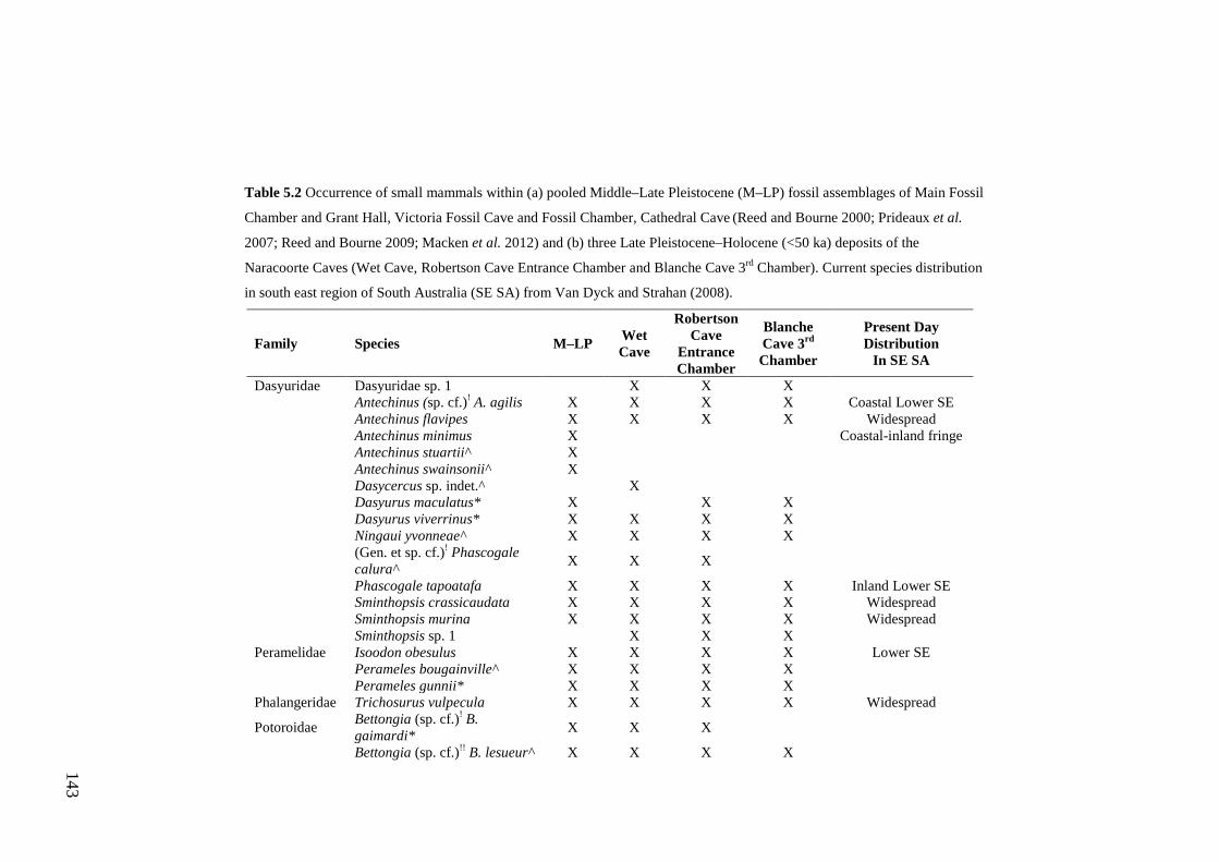
143
Table 5.2 Occurrence of small mammals within (a) pooled Middle–Late Pleistocene (M–LP) fossil assemblages of Main Fossil
Chamber and Grant Hall, Victoria Fossil Cave and Fossil Chamber, Cathedral Cave (Reed and Bourne 2000; Prideaux et al.
2007; Reed and Bourne 2009; Macken et al. 2012) and (b) three Late Pleistocene–Holocene (<50 ka) deposits of the
Naracoorte Caves (Wet Cave, Robertson Cave Entrance Chamber and Blanche Cave 3rd Chamber). Current species distribution
in south east region of South Australia (SE SA) from Van Dyck and Strahan (2008).
Family Species M–LP Wet Cave
Robertson Cave
Entrance Chamber
Blanche Cave 3rd Chamber
Present Day Distribution
In SE SA
Dasyuridae Dasyuridae sp. 1 X X X Antechinus (sp. cf.)! A. agilis X X X X Coastal Lower SE Antechinus flavipes X X X X Widespread Antechinus minimus X Coastal-inland fringe Antechinus stuartii^ X Antechinus swainsonii^ X Dasycercus sp. indet.^ X Dasyurus maculatus* X X X Dasyurus viverrinus* X X X X Ningaui yvonneae^ X X X X
(Gen. et sp. cf.)! Phascogale calura^ X X X
Phascogale tapoatafa X X X X Inland Lower SE Sminthopsis crassicaudata X X X X Widespread Sminthopsis murina X X X X Widespread Sminthopsis sp. 1 X X X Peramelidae Isoodon obesulus X X X X Lower SE Perameles bougainville^ X X X X Perameles gunnii* X X X X Phalangeridae Trichosurus vulpecula X X X X Widespread
Potoroidae Bettongia (sp. cf.)! B. gaimardi* X X X
Bettongia (sp. cf.)!! B. lesueur^ X X X X
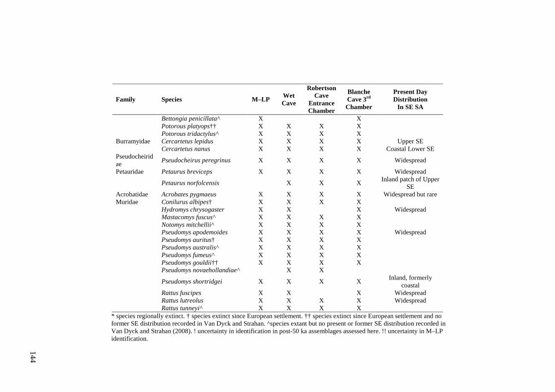
144
Family Species M–LP Wet Cave
Robertson Cave
Entrance Chamber
Blanche Cave 3rd Chamber
Present Day Distribution
In SE SA
Bettongia penicillata^ X X Potorous platyops†† X X X X Potorous tridactylus^ X X X X Burramyidae Cercartetus lepidus X X X X Upper SE Cercartetus nanus X X X X Coastal Lower SE Pseudocheiridae Pseudocheirus peregrinus X X X X Widespread
Petauridae Petaurus breviceps X X X X Widespread
Petaurus norfolcensis X X X Inland patch of Upper SE
Acrobatidae Acrobates pygmaeus X X X X Widespread but rare Muridae Conilurus albipes† X X X X Hydromys chrysogaster X X X Widespread Mastacomys fuscus^ X X X X Notomys mitchellii^ X X X X Pseudomys apodemoides X X X X Widespread Pseudomys auritus† X X X X Pseudomys australis^ X X X X Pseudomys fumeus^ X X X X Pseudomys gouldii†† X X X X Pseudomys novaehollandiae^ X X
Pseudomys shortridgei X X X X Inland, formerly coastal
Rattus fuscipes X X X Widespread Rattus lutreolus X X X X Widespread Rattus tunneyi^ X X X X
* species regionally extinct. † species extinct since European settlement. †† species extinct since European settlement and no former SE distribution recorded in Van Dyck and Strahan. ^species extant but no present or former SE distribution recorded in Van Dyck and Strahan (2008). ! uncertainty in identification in post-50 ka assemblages assessed here. !! uncertainty in M–LP identification.
145
Discussion
Late Quaternary small mammal diversity Despite the limitations presented by examining small mammal diversity across the
entire temporal span of the fossil assemblages, examination of existing and new fossil
assemblages from Wet, Roberson and Blanche Caves has resulted in significant
revision of the diversity of small mammals within the NCWHA for the late Quaternary
period from c. 50 ka. This revision provides a more accurate baseline from which long-
term patterns of species occurrence from the Middle Pleistocene to the present can be
examined. Of the eight species previously un-recorded from the assemblages of Wet,
Robertson and Blanche Caves, five were identified in this study (Antechinus sp. cf. A.
agilis, Dasyurus maculatus, Phascogale calura, Bettongia penicillata and Potorous
tridactylus), confirming their persistence, albeit rarity in some cases, into the Late
Pleistocene period to at least c. 50 ka.
Three species (Antechinus minimus, A. stuartii and A. swainsonii) were not identified
in the studied assemblages but are present in assemblages of the NCWHA dated older
than c. 70 ka (Smith, 1972; Reed and Bourne, 2000; Prideaux et al., 2007; Macken et
al., 2012). Reed and Bourne (, 2000) suggested that identification of Antechinus
species from NCWHA deposits may require revision, particularly as A. minimus, A.
stuartii and A. swainsonii were only known from single deposits at the time of their
publication. Subsequent analysis of additional NCWHA deposits has resulted in
identification of these taxa from other assemblages (Prideaux et al., 2007; Macken et
al., 2012). However, as a result of the challenges associated with differentiating A.
stuartii and A. agilis in fossil material (Reed and Bourne, 2000; Macken, 2009), the
true diversity of this genus in the NCWHA fossil record remains uncertain and
warrants further investigation. The isolation of two unknown dasyurid taxa,
Dasyuridae sp. 1 and Sminthopsis sp. 1 highlights challenges associated with
differentiating fossil material at both a generic and species level. Specimens assigned
to these categories may represent new, undescribed taxa or morphological variants of
known taxa.
If the identification of A. minimus, A. stuartii and A. swainsonii in the older Middle to
Late Pleistocene assemblages of Victoria Fossil and Cathedral Caves is correct, their
absence in Wet, Robertson and Blanche Caves suggests local decline in Dasyuridae
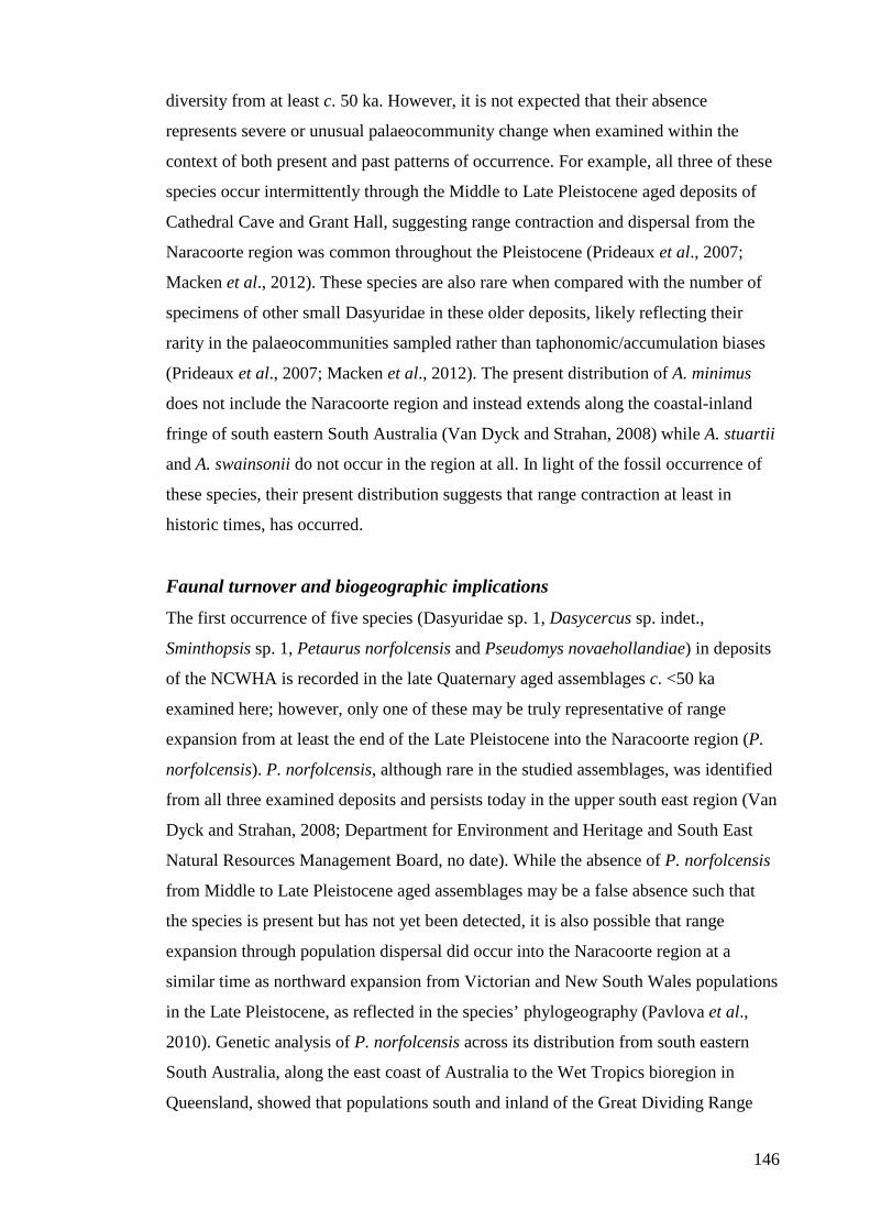
146
diversity from at least c. 50 ka. However, it is not expected that their absence
represents severe or unusual palaeocommunity change when examined within the
context of both present and past patterns of occurrence. For example, all three of these
species occur intermittently through the Middle to Late Pleistocene aged deposits of
Cathedral Cave and Grant Hall, suggesting range contraction and dispersal from the
Naracoorte region was common throughout the Pleistocene (Prideaux et al., 2007;
Macken et al., 2012). These species are also rare when compared with the number of
specimens of other small Dasyuridae in these older deposits, likely reflecting their
rarity in the palaeocommunities sampled rather than taphonomic/accumulation biases
(Prideaux et al., 2007; Macken et al., 2012). The present distribution of A. minimus
does not include the Naracoorte region and instead extends along the coastal-inland
fringe of south eastern South Australia (Van Dyck and Strahan, 2008) while A. stuartii
and A. swainsonii do not occur in the region at all. In light of the fossil occurrence of
these species, their present distribution suggests that range contraction at least in
historic times, has occurred.
Faunal turnover and biogeographic implications The first occurrence of five species (Dasyuridae sp. 1, Dasycercus sp. indet.,
Sminthopsis sp. 1, Petaurus norfolcensis and Pseudomys novaehollandiae) in deposits
of the NCWHA is recorded in the late Quaternary aged assemblages c. <50 ka
examined here; however, only one of these may be truly representative of range
expansion from at least the end of the Late Pleistocene into the Naracoorte region (P.
norfolcensis). P. norfolcensis, although rare in the studied assemblages, was identified
from all three examined deposits and persists today in the upper south east region (Van
Dyck and Strahan, 2008; Department for Environment and Heritage and South East
Natural Resources Management Board, no date). While the absence of P. norfolcensis
from Middle to Late Pleistocene aged assemblages may be a false absence such that
the species is present but has not yet been detected, it is also possible that range
expansion through population dispersal did occur into the Naracoorte region at a
similar time as northward expansion from Victorian and New South Wales populations
in the Late Pleistocene, as reflected in the species’ phylogeography (Pavlova et al.,
2010). Genetic analysis of P. norfolcensis across its distribution from south eastern
South Australia, along the east coast of Australia to the Wet Tropics bioregion in
Queensland, showed that populations south and inland of the Great Dividing Range
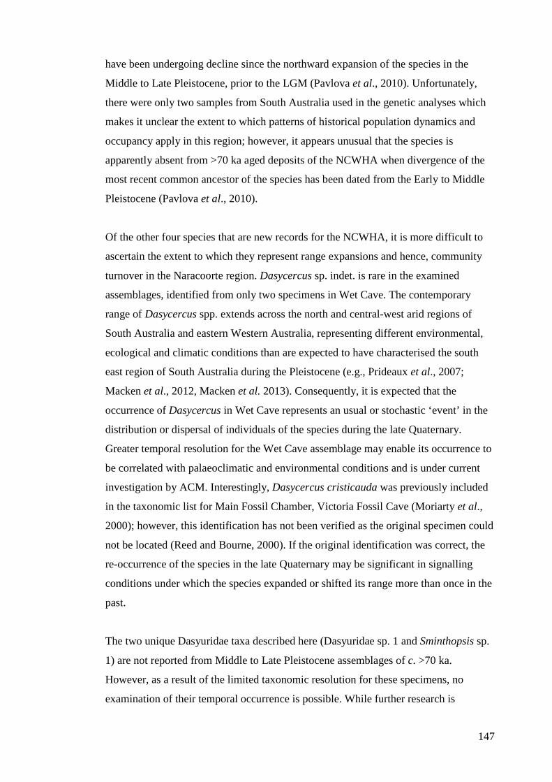
147
have been undergoing decline since the northward expansion of the species in the
Middle to Late Pleistocene, prior to the LGM (Pavlova et al., 2010). Unfortunately,
there were only two samples from South Australia used in the genetic analyses which
makes it unclear the extent to which patterns of historical population dynamics and
occupancy apply in this region; however, it appears unusual that the species is
apparently absent from >70 ka aged deposits of the NCWHA when divergence of the
most recent common ancestor of the species has been dated from the Early to Middle
Pleistocene (Pavlova et al., 2010).
Of the other four species that are new records for the NCWHA, it is more difficult to
ascertain the extent to which they represent range expansions and hence, community
turnover in the Naracoorte region. Dasycercus sp. indet. is rare in the examined
assemblages, identified from only two specimens in Wet Cave. The contemporary
range of Dasycercus spp. extends across the north and central-west arid regions of
South Australia and eastern Western Australia, representing different environmental,
ecological and climatic conditions than are expected to have characterised the south
east region of South Australia during the Pleistocene (e.g., Prideaux et al., 2007;
Macken et al., 2012, Macken et al. 2013). Consequently, it is expected that the
occurrence of Dasycercus in Wet Cave represents an usual or stochastic ‘event’ in the
distribution or dispersal of individuals of the species during the late Quaternary.
Greater temporal resolution for the Wet Cave assemblage may enable its occurrence to
be correlated with palaeoclimatic and environmental conditions and is under current
investigation by ACM. Interestingly, Dasycercus cristicauda was previously included
in the taxonomic list for Main Fossil Chamber, Victoria Fossil Cave (Moriarty et al.,
2000); however, this identification has not been verified as the original specimen could
not be located (Reed and Bourne, 2000). If the original identification was correct, the
re-occurrence of the species in the late Quaternary may be significant in signalling
conditions under which the species expanded or shifted its range more than once in the
past.
The two unique Dasyuridae taxa described here (Dasyuridae sp. 1 and Sminthopsis sp.
1) are not reported from Middle to Late Pleistocene assemblages of c. >70 ka.
However, as a result of the limited taxonomic resolution for these specimens, no
examination of their temporal occurrence is possible. While further research is
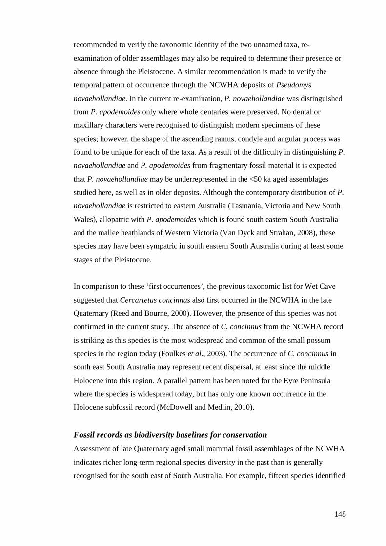
148
recommended to verify the taxonomic identity of the two unnamed taxa, re-
examination of older assemblages may also be required to determine their presence or
absence through the Pleistocene. A similar recommendation is made to verify the
temporal pattern of occurrence through the NCWHA deposits of Pseudomys
novaehollandiae. In the current re-examination, P. novaehollandiae was distinguished
from P. apodemoides only where whole dentaries were preserved. No dental or
maxillary characters were recognised to distinguish modern specimens of these
species; however, the shape of the ascending ramus, condyle and angular process was
found to be unique for each of the taxa. As a result of the difficulty in distinguishing P.
novaehollandiae and P. apodemoides from fragmentary fossil material it is expected
that P. novaehollandiae may be underrepresented in the <50 ka aged assemblages
studied here, as well as in older deposits. Although the contemporary distribution of P.
novaehollandiae is restricted to eastern Australia (Tasmania, Victoria and New South
Wales), allopatric with P. apodemoides which is found south eastern South Australia
and the mallee heathlands of Western Victoria (Van Dyck and Strahan, 2008), these
species may have been sympatric in south eastern South Australia during at least some
stages of the Pleistocene.
In comparison to these ‘first occurrences’, the previous taxonomic list for Wet Cave
suggested that Cercartetus concinnus also first occurred in the NCWHA in the late
Quaternary (Reed and Bourne, 2000). However, the presence of this species was not
confirmed in the current study. The absence of C. concinnus from the NCWHA record
is striking as this species is the most widespread and common of the small possum
species in the region today (Foulkes et al., 2003). The occurrence of C. concinnus in
south east South Australia may represent recent dispersal, at least since the middle
Holocene into this region. A parallel pattern has been noted for the Eyre Peninsula
where the species is widespread today, but has only one known occurrence in the
Holocene subfossil record (McDowell and Medlin, 2010).
Fossil records as biodiversity baselines for conservation Assessment of late Quaternary aged small mammal fossil assemblages of the NCWHA
indicates richer long-term regional species diversity in the past than is generally
recognised for the south east of South Australia. For example, fifteen species identified
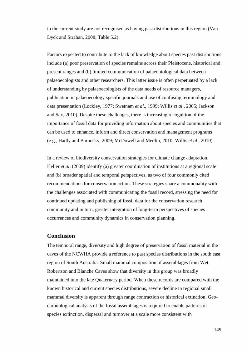
149
in the current study are not recognised as having past distributions in this region (Van
Dyck and Strahan, 2008; Table 5.2).
Factors expected to contribute to the lack of knowledge about species past distributions
include (a) poor preservation of species remains across their Pleistocene, historical and
present ranges and (b) limited communication of palaeontological data between
palaeoecologists and other researchers. This latter issue is often perpetuated by a lack
of understanding by palaeoecologists of the data needs of resource managers,
publication in palaeoecology specific journals and use of confusing terminology and
data presentation (Lockley, 1977; Swetnam et al., 1999; Willis et al., 2005; Jackson
and Sax, 2010). Despite these challenges, there is increasing recognition of the
importance of fossil data for providing information about species and communities that
can be used to enhance, inform and direct conservation and management programs
(e.g., Hadly and Barnosky, 2009; McDowell and Medlin, 2010; Willis et al., 2010).
In a review of biodiversity conservation strategies for climate change adaptation,
Heller et al. (2009) identify (a) greater coordination of institutions at a regional scale
and (b) broader spatial and temporal perspectives, as two of four commonly cited
recommendations for conservation action. These strategies share a commonality with
the challenges associated with communicating the fossil record, stressing the need for
continued updating and publishing of fossil data for the conservation research
community and in turn, greater integration of long-term perspectives of species
occurrences and community dynamics in conservation planning.
Conclusion The temporal range, diversity and high degree of preservation of fossil material in the
caves of the NCWHA provide a reference to past species distributions in the south east
region of South Australia. Small mammal composition of assemblages from Wet,
Robertson and Blanche Caves show that diversity in this group was broadly
maintained into the late Quaternary period. When these records are compared with the
known historical and current species distributions, severe decline in regional small
mammal diversity is apparent through range contraction or historical extinction. Geo-
chronological analysis of the fossil assemblages is required to enable patterns of
species extinction, dispersal and turnover at a scale more consistent with
150
palaeoclimatic and environmental change to be examined. However, the species
identification and registration data reported here provides a valuable basis for these
future analyses and a reference for ecologists, conservation managers and others on the
past distribution of small mammal taxa in south eastern South Australia.
Acknowledgements We acknowledge colleagues and other workers who have contributed to the wealth of
fossil material and knowledge on Pleistocene faunas and deposits of the Naracoorte
Caves, including but not limited to Drs Gavin Prideaux and Rod Wells; Steve Bourne,
Matt McDowell, Tegan Laslett and students, volunteers and staff of the Naracoorte
Caves of the last 40 years. ACM thanks Graham Medlin, Matt McDowell and Alex
Baynes for invaluable advice and guidance in small mammal identification and David
Stemmer and Sandy Ingleby for providing access to mammal collections of the South
Australia Museum and Australia Museum respectively. Grant Gully provided
assistance with specimen imaging while Dr Gavin Prideaux kindly provided the
equipment. EHR would like to acknowledge Steve Bourne for his part in the RCEC
project and Dr Stewart Fallon, ANU Radiocarbon Dating Centre for RCEC AMS
radiocarbon determinations. Thanks are also due to Gavin Prideaux, Aaron Camens,
Maria Zammit, Nic Rawlence, Matt McDowell and James Moore for helpful
discussions. ACM wishes to thank Alex Baynes, Rod Wells, Gilbert Price, Graham
Medlin and an anonymous reviewer for constructive comments on a previous version
of the manuscript. EHR acknowledges the following funding sources for the RCEC
excavation: major funding via the Federal Government Caring for Our Country grant
OC11-00487 and part funding for the project, “Biodiversity and vegetation change at
Naracoorte SA during the last 10,000 years” provided by the Nature Foundation SA
Inc.

151
6. Late glacial reorganisation of a small mammal
palaeocommunity in southern Australia reveals thresholds
of change
Citation Macken, A.C. & Reed, E.H. (2013) Late glacial reorganisation of a small mammal
palaeocommunity in southern Australia reveals thresholds of change. Submitted
manuscript (In Review, Ecological Monographs).
Contribution of Authors Amy Macken:
• Devised and planned the project.
• Identified and registered the specimens from Wet and Blanche Caves used
in the research presented in the manuscript.
• Conducted all faunal analyses.
• Prepared the manuscript for publication.
Elizabeth Reed:
• Discussed research with AM and assisted with planning.
• Provided comments on the manuscript.
• Supplied pollen data from Blanche Cave as published in Darrénougué et al.
(2009), for presentation in Fig. 6.12.
Signed .................................................................................. Date ............................
Amy Macken
School of Biological Sciences, Flinders University
Signed .................................................................................. Date ............................
Elizabeth Reed
School of Biological Sciences, Flinders University
152
Abstract Natural variation in ecological systems is often argued as the mechanism by which
ecosystems adapt and reorganise in response to disturbance, whilst maintaining
overall identity and functional capacity. Here, we studied the statistical and
ecological significance of natural variation in species richness, composition,
structure and relative abundance of species in two contemporaneous small mammal
fossil assemblages of late Quaternary age (c. 51.4 to 10.2 kyr BP) in south-eastern
South Australia. We asked: Did the palaeocommunity reorganise in response to
climate change associated with the last glacial cycle? How did variation in different
ecological variables contribute to the persistence or reorganisation of the
palaeocommunity, and, how did sampling variation within and between sites, and
temporal resolution, impact patterns detected in the fossil assemblages? Our results
show that the characteristics of the small mammal palaeocommunity were similar
between the two sites and that they were generally stable through the early glacial
period and last glacial maximum at the temporal scales at which the assemblages
were preserved. Thereafter, the assemblages showed evidence of change in the
rank-order abundance of constituent taxa from c. 17.1 to 10.2 kyr BP (95% CI: 17.4
to 9.2 kyr BP). At a finer temporal scale, palaeocommunity reorganisation was
revealed for the first time through the late glacial period based on significant change
in species richness. A nearby marine-core record suggests that this shift (dated from
c. 17.1 to 16.7 kyr BP; 95% CI: 17.4 to 16.2 kyr BP) was associated with sea-
surface temperatures (SSTs) warming past 16°C, post-dating the onset of warming
following the LGM by c. 1 to 3 kyrs. A second likely palaeocommunity shift is
reflected in the low rank-order abundance correlation of local palaeocommunity
samples from c. 10.8 to 10.5 kyr BP (95% CI: 11.2 to 10.9 kyr BP). This shift was
associated with continued warming of mean SSTs past 18°C. While the onset of
rapid warming was not directly correlated with palaeocommunity change, the fauna
appear to have been sensitive to specific temperature thresholds and prolonged
relative aridity. These extrinsic factors were important in initiating structural
changes that scaled through from individual species to the whole palaeocommunity.
Keywords climate change, mammals, palaeocommunity, persistence, Quaternary,
resilience, scale, similarity, variability
153
Introduction Concern about the impacts of climate change on biodiversity has led to an increased
need for long-term perspectives of ecosystems and their variability through time
(Froyd and Willis 2008). Natural variation in ecological systems is characterised by
fluctuations and/or trends in community and system attributes, condition and/or
processes (Landres et al. 1999). Such change is argued to provide an ecological
‘buffer’ that allows ecosystems to undergo turnover and reorganise in response to
external pressures, whilst maintaining ecological functions, structure, connections
and identity (Holling and Meffe 1996; Folke et al. 2004; Walker et al. 2004). The
latter aspect is at the heart of most ecological definitions of resilience, that is, how
much pressure or change an ecological system can withstand before it shifts to a
new, alternative steady-state (Holling 1996; Walker et al. 2009). Consequently,
understanding and managing natural variation in ecological systems at different
scales is increasingly being integrated into biodiversity conservation strategies.
However, despite an increased focus on natural variation in biodiversity
management and ecological literature (Landres et al. 1999; Micheli et al. 1999;
Lundberg et al. 2000; Roche et al. 2011; Walker et al. 2004), our ability to
understand patterns of natural variation is limited by the short duration of many
ecological studies, extensive habitat fragmentation, species loss and subsequent
ecosystem disruption (Swetnam et al. 1999). These factors also restrict our
knowledge of the interaction of ecosystem changes with the long-term persistence
or loss of different ecosystem attributes over time (Magurran and Henderson 2010).
The challenges associated with measuring natural variation in ecosystems can be
addressed using empirical data on environmental, climatic and ecological change
preserved in palaeoecological assemblages. Such sources are commonly used as a
reference to the normal, pre-human extent of natural variation expressed in marine,
aquatic and terrestrial ecosystems (e.g., Di Michelle et al. 2004; Hadly and
Barnosky 2009; Willis et al. 2010; Rull 2012). Baseline data from past ecosystems
provided by palaeoecological records have been used to (a) inform predictions
about climate change responses and thresholds based on ecological and climatic
variability, (b) identify the combinations of biotic and abiotic processes that most
contributed to ecological resilience in the past and where these are likely to occur
154
under future climate change scenarios, and (c) provide insights on novel, or non-
analogous communities and their management (Willis et al. 2010).
Fossil assemblages in the World Heritage listed Naracoorte Caves in south-eastern
South Australia are widely recognised for their scientific and natural history values,
preserving a diverse vertebrate fauna and palaeoclimatic history spanning the last c.
500 kyrs (Wells et al. 1984; Ayliffe et al. 1998; Reed and Bourne 2000; Prideaux et
al. 2007; Macken et al. 2012; Fig. 6.1). Recent study of deposits of Late Pleistocene
(<50 kyrs) age show that some sites also preserve a record of local vegetation
(Darrénougué et al. 2009), which combined with the faunal record, presents an
opportunity to examine the responses, thresholds and persistence of different
ecosystem variables with time for this locality.
A striking feature of the described Naracoorte mammal faunas is the general
consistency of community composition through the Pleistocene, particularly when
compared with mammal faunas from other localities such as Middle Pleistocene
north-eastern Queensland (Hocknull et al. 2007). The limited evidence presented
for faunal change in the Naracoorte fossil record has been significant in discussions
of faunal dynamics through the Pleistocene. For example, the apparent lack of
faunal change recorded in the Naracoorte Caves reported by Moriarty et al. (2000)
has been used as evidence that interglacial-glacial transitions did not contribute to
megafaunal extinction in Australia (Barnosky et al. 2004) and that Pleistocene
climate changes did not impact mammalian faunas to the same extent as the Late
Pleistocene–Holocene transition (Koch and Barnosky 2006).
The assumption of long-term stability of the mammal community through the
Pleistocene was first challenged by Prideaux et al. (2007) and later Macken et al.
(2012) who showed that the relative abundance of species within assemblages of the
Naracoorte Caves varied through glacial-interglacial cycles of the Middle and Late
Pleistocene. Additionally, changes in specimen density and species
presence/absence demonstrated in these studies showed that the ranges of some
species alternately expanded and contracted from the Naracoorte region through the
Pleistocene.
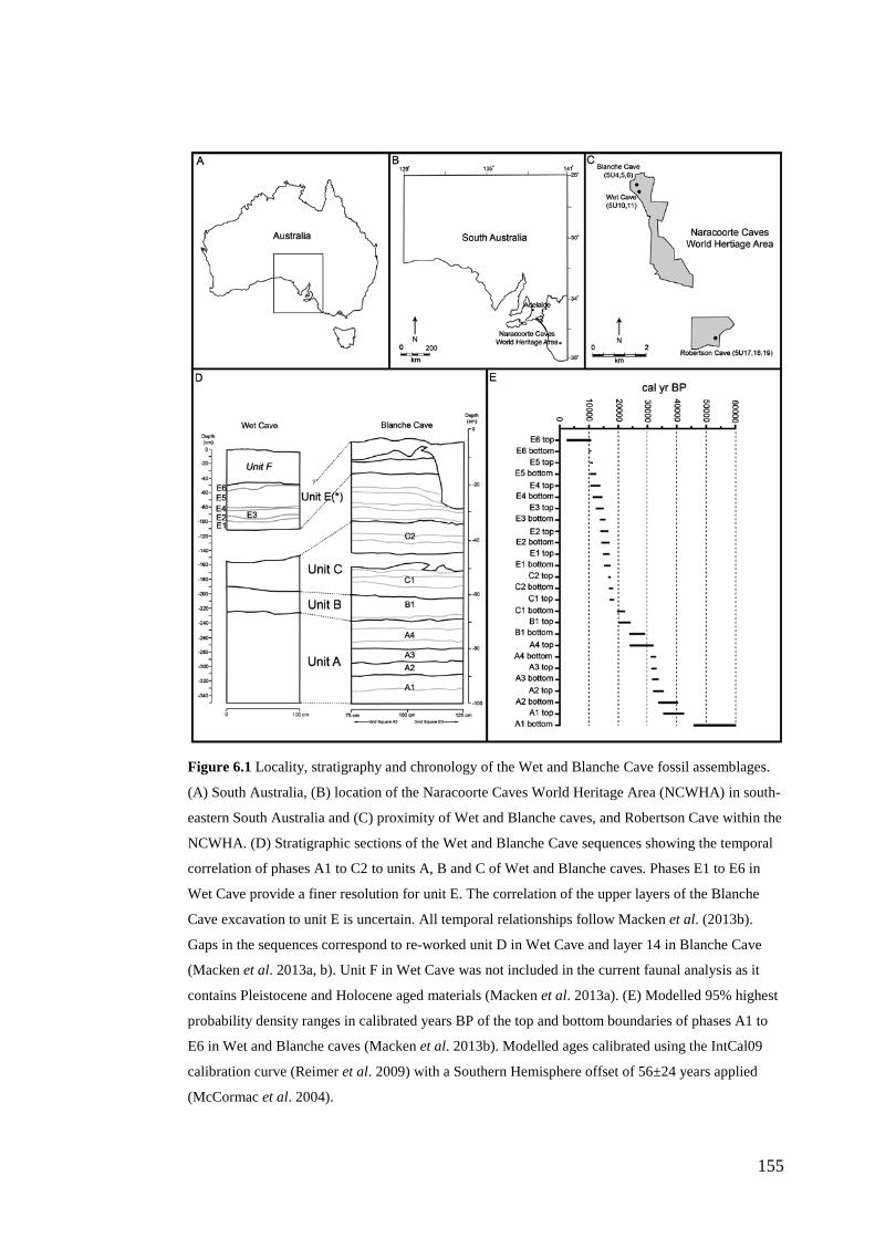
155
Figure 6.1 Locality, stratigraphy and chronology of the Wet and Blanche Cave fossil assemblages.
(A) South Australia, (B) location of the Naracoorte Caves World Heritage Area (NCWHA) in south-
eastern South Australia and (C) proximity of Wet and Blanche caves, and Robertson Cave within the
NCWHA. (D) Stratigraphic sections of the Wet and Blanche Cave sequences showing the temporal
correlation of phases A1 to C2 to units A, B and C of Wet and Blanche caves. Phases E1 to E6 in
Wet Cave provide a finer resolution for unit E. The correlation of the upper layers of the Blanche
Cave excavation to unit E is uncertain. All temporal relationships follow Macken et al. (2013b).
Gaps in the sequences correspond to re-worked unit D in Wet Cave and layer 14 in Blanche Cave
(Macken et al. 2013a, b). Unit F in Wet Cave was not included in the current faunal analysis as it
contains Pleistocene and Holocene aged materials (Macken et al. 2013a). (E) Modelled 95% highest
probability density ranges in calibrated years BP of the top and bottom boundaries of phases A1 to
E6 in Wet and Blanche caves (Macken et al. 2013b). Modelled ages calibrated using the IntCal09
calibration curve (Reimer et al. 2009) with a Southern Hemisphere offset of 56±24 years applied
(McCormac et al. 2004).
156
The greater chronological control, finer temporal resolution and more adequate and
quantitative faunal sampling in these studies facilitated rigorous analysis of faunal
trends with time and were fundamental in revealing the faunal changes that were
previously obscured. Further, the patterns of change observed in the Naracoorte
mammal record were consistent with observations elsewhere that natural variability,
and hence, our perception of stability in ecological systems, is dependent upon not
only the scales (temporal, spatial and ecological) at which they are observed (Rahel
1990; Di Michele et al. 2004; Devictor and Robert 2009), but also sampling
variance which can obscure or enhance temporal signals of variability or persistence
(Bennington and Bambach 1996).
Scale and sampling variance are critical to not only the nature of the relationship
between natural variation and persistence of faunal communities with time, but how
they may be detected and interpreted from long-term ecological records. For
example, as demonstrated by Rahel (1990), community composition and structure
(rank-order abundance) may be highly persistent, but the abundances of constituent
taxa may vary significantly with space and time. Further, Magurran and Henderson
(2010) suggested that variation in the abundances of individual species may
contribute to the overall stability of the community, highlighting a complex
interplay between variation and persistence across scales. Changes in the relative
abundance of species may also be considered “early warning signs” of
environmental impacts on ecosystems (Hadly and Barnosky 2009; p. 47),
highlighting the significance of such responses when monitoring climate change
impacts on biodiversity.
From a conservation perspective, these observations raise important questions about
the relationship between natural variation and persistence of faunal communities:
when does variability at different ecological scales represent, or lead to, a shift to a
new community type, and hence the crossing of resilience thresholds? What has
been the capacity of faunal communities and populations to resist, recover, adapt or
transform in response to past climate changes or other disturbances? Despite the
urgent need for appropriate biodiversity conservation strategies, our capacity to
address these questions is limited by a lack of knowledge about (a) how faunal
communities change over different time scales in response to disturbance (including
157
climate change), (b) the natural range of variability expressed by an ecosystem at
different spatial, temporal and ecological scales, (c) the ecological, environmental
and climatic thresholds beyond which ecosystems change state and (d) how
sampling variance (‘noise’) is differentiated from true variation (‘signal’) in
community dynamics from long-term ecological records (Willis et al. 2005; 2007;
NBSRTG 2009).
Here, we examine natural variation in a small mammal palaeocommunity preserved
in two proximal, contemporaneous small mammal fossil assemblages of the
Naracoorte Caves (Fig. 6.1; Table 6.1). These sites preserve bone-rich, well
stratified and chronologically constrained fossil assemblages of late Quaternary age,
providing an opportunity to examine natural variation of many extant taxa which
today persist in communities non-analogous to those of Pleistocene Naracoorte
(Macken et al. 2012; Macken and Reed 2013).
The aims of this research were to (a) examine how sampling variation within and
between sites, and temporal resolution affect perceived patterns of variation and/or
stability in the fossil assemblages, (b) determine if and how the palaeocommunity
reorganised in response to climate change associated with the last glacial cycle, and
(c) identify how variation in different ecological variables contributed to the
persistence or reorganisation of the palaeocommunity at different scales (temporal
and ecological). Using local and regional palaeoclimatic and environmental
indicators (e.g., estimated sea-surface temperatures from offshore south-eastern
South Australia and a vegetation record preserved in Blanche Cave), we also
identify climatic and environmental changes associated with significant episodes of
faunal turnover recorded in the fossil assemblages.
We use the terminology of Bennington and Bambach (1996) in describing the
assemblages sampled from single stratigraphic units or layers as a ‘local
palaeocommunity’. We also use the terms ‘palaeocommunity’ and
‘palaeocommunity type’ to describe groups of samples that are statistically
indistinguishable and groups of samples that are similar but are statistically
distinguishable, respectively (Bennington and Bambach 1996). These and other
palaeoecology-specific and numeric terms used throughout the text are described in
158
Table 6.2. We recognise that given the extent of time-averaging, biasing and
information loss through taphonomic processes in fossil assemblages, a local
palaeocommunity is not equivalent to a local community observed in neontolgoical
studies where contemporaneity can be established. However, this terminology
provides a useful basis for describing the different types of samples examined from
the fossil assemblages and an ecological hierarchy from which to describe the
biological significance of natural variation observed with time.
Study region The South East region of South Australia is today characterised climatically by
cool, wet winters and long, mild, dry summers, placing it in the temperate climate
zone (Hopton 2003). Annual rainfall and mean maximum temperatures range from
c. 775 mm and 19oC in Mount Gambier to c. 470 mm and c. 22oC in Keith, located
in the southern and northern ends of the region respectably. Naracoorte is located in
the centre of south-eastern South Australia and has an annual rainfall of c. 580 mm
and mean maximum temperature of c. 21oC (Hopton 2003). Mean sea-surface
temperature along the western coastal edge of the region is in the range of 16 to
18oC (Bureau of Meteorology, 2013). Across the region, effective precipitation
(rainfall > evaporation rate) occurs only during the winter.
The region is geomorphically complex, with a range of landforms that historically
(immediately pre-European colonisation) supported a diverse range of vegetation
communities (Croft 2003). The variety of landforms and vegetation communities
supported a diverse mammal fauna through the Pleistocene and into historical times.
Forty-one small mammal species (excluding bats) have been identified from
Naracoorte fossil sites dated from c. 50 to 1 kyr BP (Macken and Reed 2013).
Biological surveys in 1997 and museum records indicate that 26 small mammal taxa
were known from the region at the time of European arrival and through to more
recent times (Robinson et al. 2000; Foulkes et al. 2003). South-eastern South
Australia represents the western-limit of the mainland distribution of many extant
south-eastern Australian small mammal species, while others are more widespread
across the continent (Van Dyck and Strahan 2008).
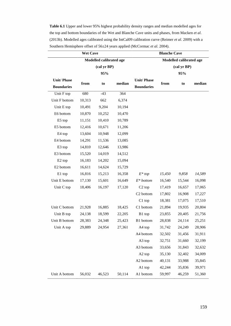
159
Table 6.1 Upper and lower 95% highest probability density ranges and median modelled ages for
the top and bottom boundaries of the Wet and Blanche Cave units and phases, from Macken et al.
(2013b). Modelled ages calibrated using the IntCal09 calibration curve (Reimer et al. 2009) with a
Southern Hemisphere offset of 56±24 years applied (McCormac et al. 2004).
Wet Cave Blanche Cave
Modelled calibrated age
(cal yr BP)
Modelled calibrated age
(cal yr BP)
95% 95%
Unit/ Phase
Boundaries from to median
Unit/ Phase
Boundaries from to median
Unit F top 680 -43 364
Unit F bottom 10,313 662 6,374
Unit E top 10,491 9,204 10,194
E6 bottom 10,870 10,252 10,470
E5 top 11,151 10,410 10,789
E5 bottom 12,416 10,671 11,206
E4 top 13,604 10,948 12,099
E4 bottom 14,291 11,536 13,085
E3 top 14,810 12,646 13,986
E3 bottom 15,520 14,019 14,512
E2 top 16,183 14,202 15,094
E2 bottom 16,611 14,624 15,729
E1 top 16,816 15,213 16,358 E* top 15,450 9,858 14,589
Unit E bottom 17,130 15,601 16,649 E* bottom 16,540 15,544 16,098
Unit C top 18,406 16,197 17,120 C2 top 17,419 16,657 17,065
C2 bottom 17,802 16,908 17,227
C1 top 18,381 17,075 17,510
Unit C bottom 21,928 16,885 18,425 C1 bottom 21,894 19,935 20,804
Unit B top 24,138 18,599 22,205 B1 top 23,855 20,405 21,756
Unit B bottom 28,383 24,348 25,423 B1 bottom 28,838 24,114 25,251
Unit A top 29,889 24,954 27,361 A4 top 31,742 24,249 28,906
A4 bottom 32,502 31,456 31,911
A3 top 32,751 31,660 32,199
A3 bottom 33,656 31,843 32,632
A2 top 35,130 32,402 34,009
A2 bottom 40,131 33,988 35,845
A1 top 42,244 35,836 39,971
Unit A bottom 56,032 46,523 50,114 A1 bottom 59,997 46,259 51,360
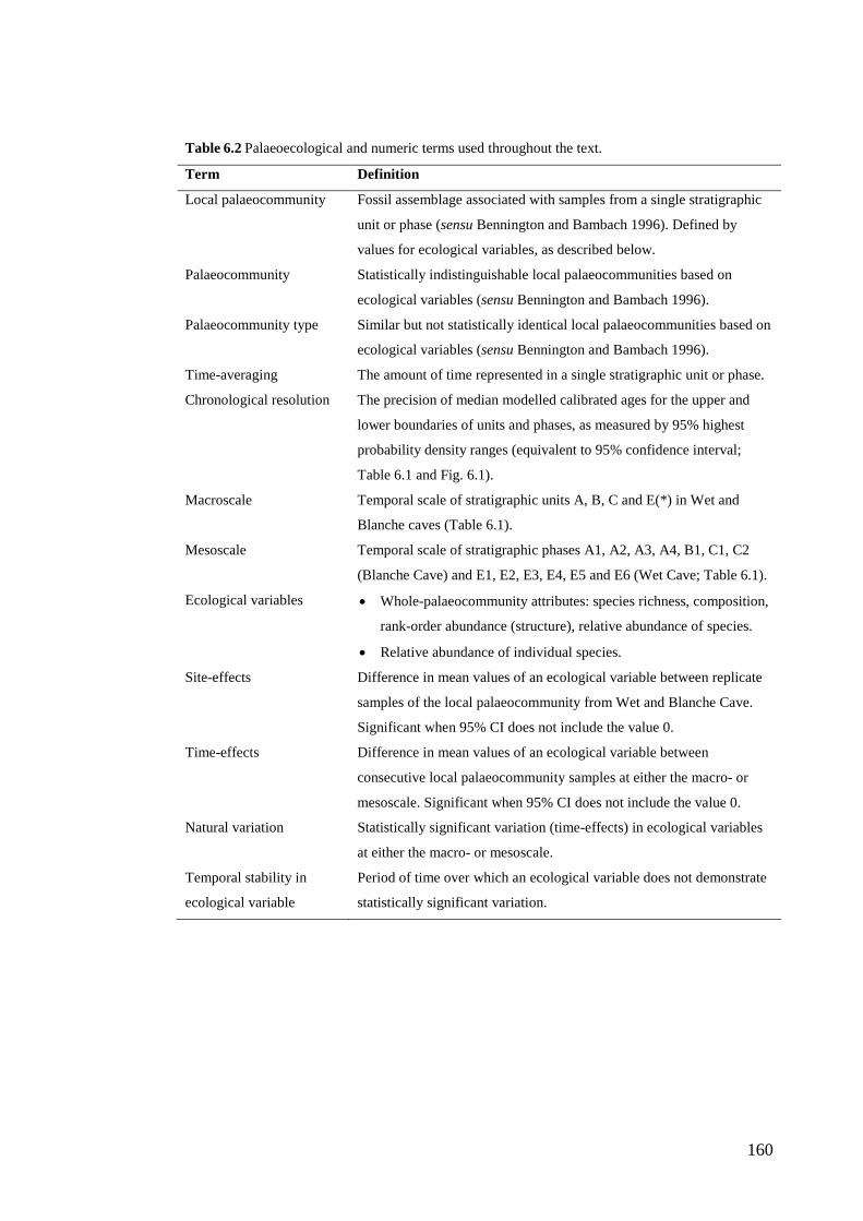
160
Table 6.2 Palaeoecological and numeric terms used throughout the text.
Term Definition
Local palaeocommunity Fossil assemblage associated with samples from a single stratigraphic
unit or phase (sensu Bennington and Bambach 1996). Defined by
values for ecological variables, as described below.
Palaeocommunity Statistically indistinguishable local palaeocommunities based on
ecological variables (sensu Bennington and Bambach 1996).
Palaeocommunity type Similar but not statistically identical local palaeocommunities based on
ecological variables (sensu Bennington and Bambach 1996).
Time-averaging The amount of time represented in a single stratigraphic unit or phase.
Chronological resolution The precision of median modelled calibrated ages for the upper and
lower boundaries of units and phases, as measured by 95% highest
probability density ranges (equivalent to 95% confidence interval;
Table 6.1 and Fig. 6.1).
Macroscale Temporal scale of stratigraphic units A, B, C and E(*) in Wet and
Blanche caves (Table 6.1).
Mesoscale Temporal scale of stratigraphic phases A1, A2, A3, A4, B1, C1, C2
(Blanche Cave) and E1, E2, E3, E4, E5 and E6 (Wet Cave; Table 6.1).
Ecological variables • Whole-palaeocommunity attributes: species richness, composition,
rank-order abundance (structure), relative abundance of species.
• Relative abundance of individual species.
Site-effects Difference in mean values of an ecological variable between replicate
samples of the local palaeocommunity from Wet and Blanche Cave.
Significant when 95% CI does not include the value 0.
Time-effects Difference in mean values of an ecological variable between
consecutive local palaeocommunity samples at either the macro- or
mesoscale. Significant when 95% CI does not include the value 0.
Natural variation Statistically significant variation (time-effects) in ecological variables
at either the macro- or mesoscale.
Temporal stability in
ecological variable
Period of time over which an ecological variable does not demonstrate
statistically significant variation.
161
Geological setting of the Naracoorte Caves The Naracoorte Caves are a complex of 26 caves distributed within an uplifted
portion of the Oligocene to Miocene aged Gambier Limestone and are located
south-east of Naracoorte (Fig. 6.1). The uplifted section of the Gambier Limestone
is overlain by the East Naracoorte Ridge, the oldest of the Pleistocene beach dune
facies which transect the South East region (Murray-Wallace et al. 2001). The caves
formed through phreatic dissolution and structural processes along joints in the
Gambier Limestone (Wells et al. 1984; Lewis et al. 2006), first opening to the
surface from at least the Middle Pleistocene (c. 530 ka) as indicated by optically
stimulated luminescence dating of bone-bearing clastic sediments from an
assemblage in Cathedral Cave (5U12 13; Prideaux et al. 2007).
There are 100 known fossil vertebrate fossil deposits ranging in age from the
Middle Pleistocene to the Holocene within the Naracoorte Caves (Macken et al.
2013a; Macken and Reed 2013). The two deposits examined here (Wet Cave
Entrance Chamber: 5U10 and Blanche Cave 3rd Chamber: 5U6) are largely
contemporaneous, together spanning the last glacial cycle from c. 51.4 to 10.2 kyr
BP (Darrénougué et al. 2009; St. Pierre et al. 2012; Macken et al. 2013a, b).
The Naracoorte Caves are registered with the Australian Karst Index (Matthews
1985) and are identified by unique cave numbers (e.g., 5U10 11), referred to in text.
‘5’ identifies the state of South Australia, ‘U’ the Upper South East and the
numbers (e.g. 10 11) indicate entrances associated with each registered cave.
Chronology and stratigraphy of Wet and Blanche caves The stratigraphic and geochronological contexts of the fossil deposits of Wet and
Blanche caves are described in Darrénougué et al. (2009), St Pierre et al. (2009), St
Pierre et al. (2012) and Macken et al. (2013a). Bayesian age-depth models for the
two deposits were developed by Macken et al. (2013b) and were used as the
chronological and stratigraphic framework for the faunal analyses presented here
(Fig. 6.1; Table 6.1). The Bayesian age-depth models integrated stratigraphic
information for the two sites and 14C determinations from charcoal collected across
the sequences. A total of 20 14C determinations were used to build the Wet Cave
model and 40 for the Blanche Cave model (Macken et al. 2013b). We discuss U/Th
162
dates from speleothem straws (St Pierre et al. 2009, 2012) in conjunction with the
age-models and 14C determinations in terms of potential reworking of sediments
and bone material in the later sections of the paper. Here we provide a general
description of the depositional sequences and the age-models as a context for the
temporal division and relationships of the fossil assemblages within and between
the two sites.
The Wet Cave fossil deposit is composed of four un-reworked depositional units
(A, B, C and E; Fig. 6.1; Table 6.1). Unit D and the uppermost unit F contain
reworked sedimentary and bone material older than the depositional context and
were consequently excluded from the faunal analysis. Units A, B and C lack
internal laminations and provide macroscale, time-averaged samples of the fossil
assemblage through the period from c. 50.1 to 17.1 kyr BP, with maximum
modelled durations for the units ranging from c. 30.5 to 4.5 kyrs at the 95% highest
probability density (hpd) range (Macken et al. 2013b; Table 6.1). These
depositional units correspond to broad climatic phases of the last glacial cycle
(marine isotope stage 3 (MIS-3) and last glacial maximum (LGM) in MIS-2;
Macken et al. 2013a, b). Unit E is dated to the MIS-2 deglaciation and is composed
of six layers (phases E1, oldest to E6, youngest), identified by sedimentary
characteristics and representing discrete phases of sediment and bone accumulation
(Macken et al. 2013a, b). The maximum modelled temporal durations of these
phases range from 180 to 370 years at the 95% hpd, providing a finer, mesoscale
resolution for the MIS-2 deglaciation period of c. 16.7 to 10.2 kyr BP represented
by Wet Cave unit E (Macken et al. 2013a; Fig. 6.1; Table 6.1).
The deposit in Blanche Cave closely resembles that of Wet Cave in terms of the
general sequence of sediment types through the sequence and depositional age, but
differs in the depth profile and by the number of sedimentary layers present
(Macken et al. 2013a, b). Twenty-seven sedimentary layers were originally
identified in the Blanche Cave section based on visual observation during
excavation. Following analysis of the sediments and further examination of the
stratigraphy, these layers were subsequently aggregated into seven separate phases
(A1 to C2; Table E.1 Appendix E).
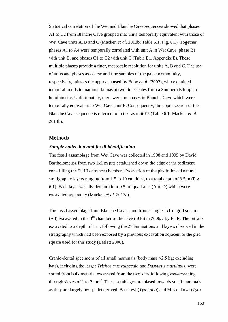
163
Statistical correlation of the Wet and Blanche Cave sequences showed that phases
A1 to C2 from Blanche Cave grouped into units temporally equivalent with those of
Wet Cave units A, B and C (Macken et al. 2013b; Table 6.1; Fig. 6.1). Together,
phases A1 to A4 were temporally correlated with unit A in Wet Cave, phase B1
with unit B, and phases C1 to C2 with unit C (Table E.1 Appendix E). These
multiple phases provide a finer, mesoscale resolution for units A, B and C. The use
of units and phases as coarse and fine samples of the palaeocommunity,
respectively, mirrors the approach used by Bobe et al. (2002), who examined
temporal trends in mammal faunas at two time scales from a Southern Ethiopian
hominin site. Unfortunately, there were no phases in Blanche Cave which were
temporally equivalent to Wet Cave unit E. Consequently, the upper section of the
Blanche Cave sequence is referred to in text as unit E* (Table 6.1; Macken et al.
2013b).
Methods
Sample collection and fossil identification The fossil assemblage from Wet Cave was collected in 1998 and 1999 by David
Bartholomeusz from two 1x1 m pits established down the edge of the sediment
cone filling the 5U10 entrance chamber. Excavation of the pits followed natural
stratigraphic layers ranging from 1.5 to 10 cm thick, to a total depth of 3.5 m (Fig.
6.1). Each layer was divided into four 0.5 m2 quadrants (A to D) which were
excavated separately (Macken et al. 2013a).
The fossil assemblage from Blanche Cave came from a single 1x1 m grid square
(A3) excavated in the 3rd chamber of the cave (5U6) in 2006/7 by EHR. The pit was
excavated to a depth of 1 m, following the 27 laminations and layers observed in the
stratigraphy which had been exposed by a previous excavation adjacent to the grid
square used for this study (Laslett 2006).
Cranio-dental specimens of all small mammals (body mass ≤2.5 kg; excluding
bats), including the larger Trichosurus vulpecula and Dasyurus maculatus, were
sorted from bulk material excavated from the two sites following wet-screening
through sieves of 1 to 2 mm2. The assemblages are biased towards small mammals
as they are largely owl-pellet derived. Barn owl (Tyto alba) and Masked owl (Tyto
164
novaehollandiae) are the most likely predatory agents responsible for the deposits
as evidenced by the presence of these species within the fossil assemblages, the
prevalence of complete skeletal elements and presence of digestive corrosion
consistent with tytonid owls (McDowell 2001; Laslett 2006). Although of greater
body mass, T. vulpecula and D. maculatus were included in the faunal analysis as
they are represented by juvenile specimens and hence, may be a component of the
largely owl-pellet derived assemblages.
For identification, cranio-dental specimens were compared with modern and sub-
fossil specimens in the South Australian Museum and modern specimens held by
the Australian Museum as described in Macken and Reed (2013). Published
descriptions of species cranio-dental morphology were also used to aid species
identification where available. Two un-diagnosed taxa were identified in the fossil
assemblages (Dasyuridae sp. 1 and Sminthopsis sp. 1) and are discussed by Macken
and Reed (2013).
Previous analysis of the Wet Cave assemblage by McDowell (2001) showed that
murids composed 81% of the fauna (c. 14,000 cranio-dental specimens). Due to this
abundance of material, murids were sub-sampled from the Wet Cave collection. For
layers where the total Number of Identified Specimens (NISP) of murids was >300
(as indicated in the data tables presented in McDowell 2001), only specimens from
quadrant A were examined, approximating 25% of the bulk material for the layer
(Macken and Reed 2013). For layers where the NISP of murids was <300,
specimens from all quadrants were identified. Marsupial NISP was determined from
the sum of specimens identified from all quadrants.
As in Wet Cave, murid cranio-dental specimens from Blanche Cave composed 80%
of the fauna (c. 18,000 cranio-dental specimens, counted during analysis) and were
sub-sampled. For layers where the number of murid specimens counted was >300,
only specimens from a random sample of 25% of the volume of bulk material for
the layer were identified (see Macken and Reed, 2013), approximating the quadrant
method used in Wet Cave. All marsupial specimens from grid square A3 were
identified.
165
All specimens identified from Wet and Blanche caves were registered to the
Flinders University fossil collection (Wet Cave: FU20000 to 20997; Blanche Cave:
FU14100 to 14685).
Faunal analysis: data standardisation The total NISP for each murid taxon in the sub-sampled layers was estimated by
multiplying the proportion of each taxon by the total murid NISP for the layer (e.g.,
Blanche Cave Layer 3 had a total counted murid NISP = 782. The sub-sampled
murid NISP for Layer 3 = 147. The proportion of Pseudomys apodemoides in the
sub-sample for Layer 3 = 0.17, based on 25 specimens identified to this taxon.
Therefore, the estimated total NISP for P. apodemoides in Layer 3 was 0.17 x 782 =
133).
We recognise that our sub-sampling strategy may have resulted in some murid taxa
not being identified from the sub-sampled layers, particularly if they were very rare
in the assemblage. We tested for such an effect by constructing rarefaction curves
for the sub-sampled layers and those where all specimens were identified.
Rarefaction curves show that for most samples, the number of species in both the
sub-sampled and completely sampled layers approaches asymptote, suggesting
negligible sampling effects (Figs. E.1 and E.2 Appendix E). We also note that the
minimum sub-sampled murid NISP from a single layer from Wet and Blanche
caves was 65, greater than the minimum NISP of any marsupial species (Wet Cave
phase E1=36). Rarefaction analysis was conducted in the palaeontological software
package PAST (Hammer et al. 2001).
NISP values of the small mammal faunas were used to calculate the local
palaeocommunity metrics detailed below and were quantified at the two time scales
(macro- and meso-) available in the deposits. For analysis, the NISP of Pseudomys
novaehollandiae was incorporated into the NISP of P. apodemoides due to the
difficulties in separating these taxa from cranio-dental specimens (Macken and
Reed 2013).
To allow for comparison of the local palaeocommunity sampled between and within
the two sites at both the macro- and meso- time scales, all samples were
166
standardised to the lowest NISP from a unit or phase (Wet Cave phase E1 = 303)
using bootstrapping, following the methods of Blois et al. (2010) and Chernick
(2008). One-thousand bootstrap samples for each unit and phase were generated by
resampling with replacement, using the proportion of each species in the original
samples as weights. Resampling was conducted in R version 2.15.1 (R Core Team,
2012).
Faunal analysis: whole-palaeocommunity and individual species variables Species richness (number of species) and evenness (probability of interspecific
encounter; PIE) were calculated using the bootstrapped, sample-size standardised
data. Richness and evenness together reflect diversity and are commonly calculated
for fossil assemblages (e.g., Blois et al. 2010; Terry 2010a, b) and modern
ecological communities (e.g., Kelly et al. 2010). Richness is generally considered to
reflect ecosystem productivity and habitat heterogeneity (Hadly and Barnosky
2009; Bateman et al. 2010) while evenness reflects the distribution of relative
abundance of species within faunal assemblages.
We also calculated the following beta diversity measures:
• Composition (species presence/absence; Jaccard similarity index),
• Species rank-order abundance (abundance rankings; Spearman’s
Rho, ρ) and
• Relative abundance of species (Bray-Curtis similarity index),
following Rahel (1990).
These metrics are commonly calculated for fossil assemblages (e.g., Terry 2010b)
and provide a nested hierarchy for evaluating the ecological extent of variation and
stability within the palaeocommunity (Belmaker and Hovers, 2011). The Jaccard
and Bray-Curtis similarity indices were calculated from the bootstrapped sample-
size standardised data using R, and Spearman’s rank-order abundance correlations
from the original, un-bootstrapped data in SPSS version 19 (IBM Corp 2010). The
95% confidence intervals of the bootstrapped sample means were calculated using
the upper and lower 2.5% percentiles of the bootstrapped distributions following
Chernick (2008) and Dalby et al. (2013). Confidence intervals for Spearman’s
167
correlation coefficients were calculated using the Fisher transformation as outlined
in Zar (1996).
The significance of mean Jaccard similarity was assessed using the upper and lower
critical values published by Real (1999). The critical values provide the probability
that an observed Jaccard index value is different from what would be expected at
random, given the number of taxa within the two samples.
The significance of Spearman’s Rho was tested against the null hypothesis that
species abundance ranks were not associated between samples (ρ=0). For all tests,
significance was assessed at α=0.01 to reduce the chance of Type 1 error associated
with multiple comparisons. We used this more conservative significance level as an
alternative to the strict adjustments enforced by more commonly used procedures
such as Bonferroni correction which can inflate the likelihood of Type 2 errors
(Verhoeven et al. 2005).
Finally, the relative abundances of individual species and associated 95%
confidence intervals were calculated using the “plus-four” method as outlined in
Agresti and Caffo (2000) and Moore and McCabe (2007). This method is preferred
to the standard confidence interval for proportions as it is less likely to produce
confidence intervals that are smaller than 95%.
Faunal analysis: site- and time-effects As the fossil assemblages are located within 500 m of each other, we tested the
similarity of the palaeocommunity preserved in each site as a basis for assessing the
reliability of observed temporal variation at the species and whole-assemblage
levels. This approach was endorsed by Bennington and Bambach (1996), but is
rarely applied to vertebrate fossil localities where typically, there is only one
assemblage available for a given time period.
Site based sampling effects were calculated for species richness and evenness as the
difference in means of the 1000 bootstrap samples for comparisons between units
A, B, C and E(*) sampled from the two sites, following Nakagawa and Cuthill
(2007) and Dalby et al. (2013). We adopted this method as it provides information
168
about the magnitude and precision of effects and is useful when multiple
comparisons are being considered (Di Stefano 2004; Nakagawa 2004; Nakagawa
and Cuthill 2007). Site-effects on the relative abundances of individual species were
quantified using the mean difference in species proportions. Site-based similarity of
the beta diversity measures were examined by calculating these measures for all
unit comparisons between the two sites (e.g., Wet Cave unit A v. Blanche Cave unit
A).
The effects of time-averaging on patterns of variability (time-effects) were
examined by studying the assemblages at the two temporal scales available in the
deposit: (a) the coarse, macroscale corresponding to broad climatic phases of the
last glacial cycle (e.g., marine isotope stage (MIS)-3, the Last Glacial Maximum
(LGM) and MIS-2 deglaciation), and (b) the finer, mesoscale of millennia or
centuries, enabling variation within these broader climatic phases to be examined.
Time-effects on species richness and evenness were quantified as the difference in
means of the 1000 bootstrap samples between consecutive units and phases within
each site. Time-effects on the relative abundances of individual species were
examined using the mean difference in proportions of consecutive units and phases.
The beta diversity measures were also calculated for consecutive units and phases.
To examine similarity amongst all units and phases and to assess overall temporal
trends at the macro- and mesoscales, we additionally used the unweighted paired-
group method of hierarchical cluster analysis based on arithmetic means, using
Jaccard and Bray-Curtis similarity (using the bootstrapped sample-size standardised
NISP values), and Spearman’s Rho (original NISP values), similar to the approach
of Belmaker and Hovers (2011). As a multivariate technique, cluster analysis
facilitated a comparison of all units and phases, rather than between consecutive
units and phases only. Although cluster analysis does not provide a test of
significance of the similarities among samples, we used bootstrapping to test the
consistency of nodes in the cluster dendrogram (1000 resamples). Nodes of ≥ 95%
support were considered to be different from random (Jackson et al. 2010). Cluster
analysis was performed in PAST version 2.02.
Given the range of depositional and post-depositional processes that can contribute
to the heterogeneity of species relative abundances between samples within a single
169
sedimentary horizon (Bennington and Bambach 1996), we additionally examined
the significance of temporal trends in species proportions using the Cochran-
Armitage test (Chi-square test for linear trend), following Zar (1996) and Cannon
(2000). The test was applied at the macroscale on those species that recorded
presences in at least three units, and at the mesoscale, on those species that occurred
in at least four phases. Cochran-Armitage tests for the effect of sample size on
observed trends in proportion data by dividing the total chi-square value into two
parts: one that is due to a linear trend in abundance and another due to departure
from linearity, such as curvilinear trends (Cannon 2001). The test was performed
with the ‘Chi-square and Cochran’s Calculator’ Microsoft Excel macro created by
Cannon. We used the Type I error rate of α=0.01 for Cochran’s test.
The statistical significance of site and time-effects was established on the a basis
that the 95% confidence interval of the effect size did not contain 0. Significant
time-effects were additionally judged on the basis that time-effect size was greater
than site-effect size (based on overlap of 95% confidence intervals of site and time-
effects), following Cumming (2009) and noting the cautions of Schenker and
Gentleman (2001). Non-statistically significant changes in community attributes
with time were considered as ‘noise,’ cautioning against over-interpretation of
ecological meaning. In contrast, given the extent of sampling variation inherent in
fossil assemblages, statistically significant variation was considered to also be
ecologically significant (‘signal’). We acknowledge that this does not mean that
non-statistically significant variation is not ecologically meaningful, only that our
confidence in the observed trends is limited by sampling variation.
Palaeoclimatic and environmental context The faunal data were compared against late Quaternary sea-surface temperatures
(SST) reconstructed from marine core MD03-2607 collected from offshore south-
eastern South Australia (Lopes dos Santos et al. 2012). SSTs were plotted at the
temporal resolution of the original core data and as mean values time-averaged over
the temporal durations of the units and phases of Wet and Blanche caves (based on
the maximum median ages of the upper and lower unit and phase boundaries; Table
6.1). Mean SST time-averaged over the upper and lower 95% hpd ranges of the top
170
and bottom boundaries of the units and phases, respectively, resulted in almost
identical values as those time-averaged within the median ages.
Pollen data from a sediment core collected from the 3rd chamber of Blanche Cave
were used as a proxy for the broad types of vegetation local to the Naracoorte Caves
over the last glacial cycle (Darrénougué et al. 2009). Mean percentages of woody,
herbaceous and woody-herbaceous taxa were calculated from samples
corresponding to each of units A, B, C and E*. The Naracoorte Cave speleothem
growth record was used as an indicator of effective moisture availability over the
late Quaternary for this locality (Ayliffe et al. 1999).
Results
Data summary Thirty-nine small mammal taxa were identified from 6,749 specimens from Wet
Cave and 7,161 from Blanche Cave units A, B, C and E* and their associated
phases (Table E.1 Appendix E). The total, murid sub-sample adjusted NISP for the
assemblages were 11,075 (Wet) and 18,216 (Blanche).
Sampling variation of the local palaeocommunity: site-effects No significant site-effects on species richness were detected between units A, B, C
and E(*) of Wet and Blanche caves (Fig. 6.2; Table 6.3). By comparison, significant
site-based sampling variation was evident in the evenness of the assemblages of
units A, B and C between the two sites (Fig. 6.2; Table 6.3).
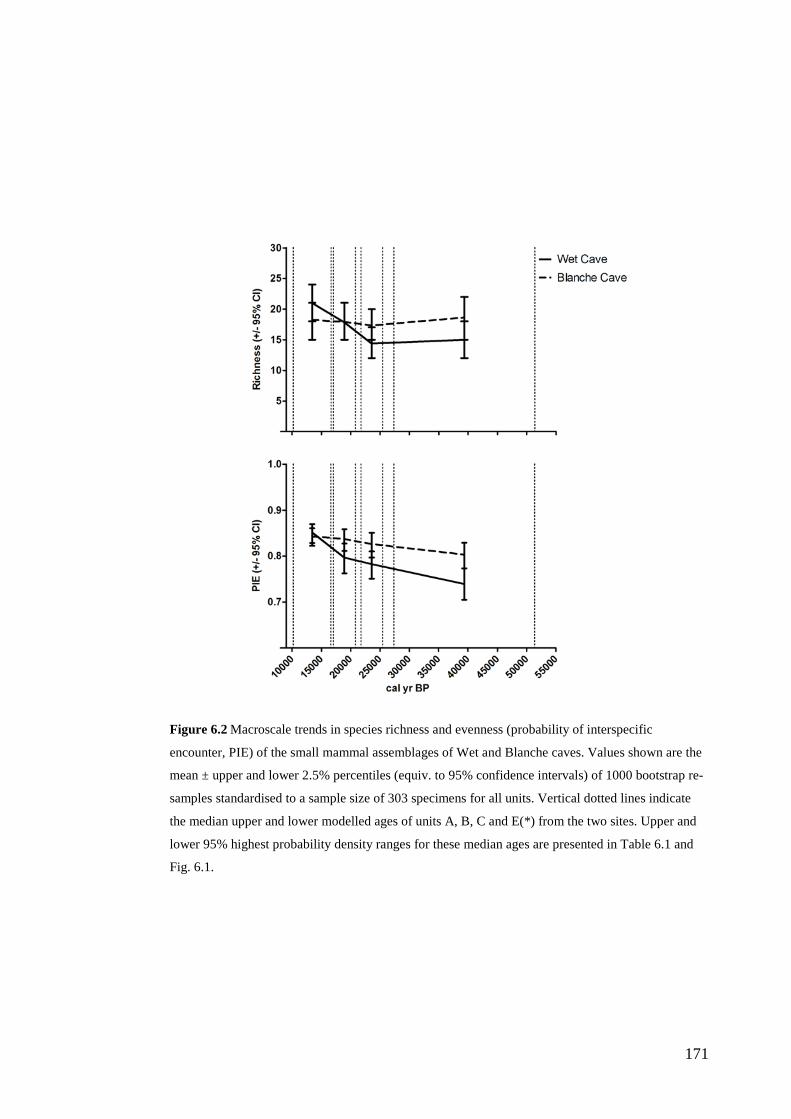
171
Figure 6.2 Macroscale trends in species richness and evenness (probability of interspecific
encounter, PIE) of the small mammal assemblages of Wet and Blanche caves. Values shown are the
mean ± upper and lower 2.5% percentiles (equiv. to 95% confidence intervals) of 1000 bootstrap re-
samples standardised to a sample size of 303 specimens for all units. Vertical dotted lines indicate
the median upper and lower modelled ages of units A, B, C and E(*) from the two sites. Upper and
lower 95% highest probability density ranges for these median ages are presented in Table 6.1 and
Fig. 6.1.
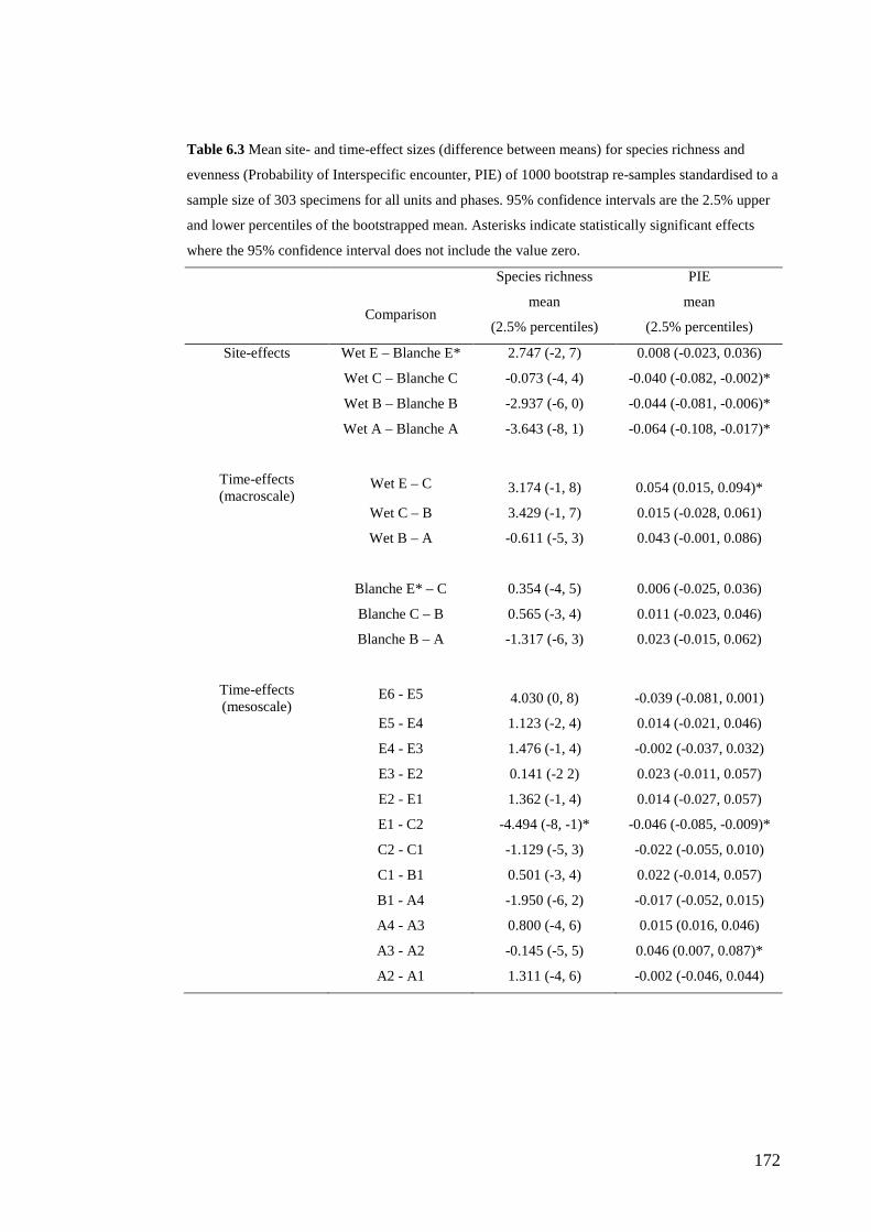
172
Table 6.3 Mean site- and time-effect sizes (difference between means) for species richness and
evenness (Probability of Interspecific encounter, PIE) of 1000 bootstrap re-samples standardised to a
sample size of 303 specimens for all units and phases. 95% confidence intervals are the 2.5% upper
and lower percentiles of the bootstrapped mean. Asterisks indicate statistically significant effects
where the 95% confidence interval does not include the value zero.
Species richness PIE
Comparison
mean
(2.5% percentiles)
mean
(2.5% percentiles)
Site-effects Wet E – Blanche E* 2.747 (-2, 7) 0.008 (-0.023, 0.036)
Wet C – Blanche C -0.073 (-4, 4) -0.040 (-0.082, -0.002)*
Wet B – Blanche B -2.937 (-6, 0) -0.044 (-0.081, -0.006)*
Wet A – Blanche A -3.643 (-8, 1) -0.064 (-0.108, -0.017)*
Time-effects (macroscale)
Wet E – C 3.174 (-1, 8) 0.054 (0.015, 0.094)*
Wet C – B 3.429 (-1, 7) 0.015 (-0.028, 0.061)
Wet B – A -0.611 (-5, 3) 0.043 (-0.001, 0.086)
Blanche E* – C 0.354 (-4, 5) 0.006 (-0.025, 0.036)
Blanche C – B 0.565 (-3, 4) 0.011 (-0.023, 0.046)
Blanche B – A -1.317 (-6, 3) 0.023 (-0.015, 0.062)
Time-effects (mesoscale)
E6 - E5 4.030 (0, 8) -0.039 (-0.081, 0.001)
E5 - E4 1.123 (-2, 4) 0.014 (-0.021, 0.046)
E4 - E3 1.476 (-1, 4) -0.002 (-0.037, 0.032)
E3 - E2 0.141 (-2 2) 0.023 (-0.011, 0.057)
E2 - E1 1.362 (-1, 4) 0.014 (-0.027, 0.057)
E1 - C2 -4.494 (-8, -1)* -0.046 (-0.085, -0.009)*
C2 - C1 -1.129 (-5, 3) -0.022 (-0.055, 0.010)
C1 - B1 0.501 (-3, 4) 0.022 (-0.014, 0.057)
B1 - A4 -1.950 (-6, 2) -0.017 (-0.052, 0.015)
A4 - A3 0.800 (-4, 6) 0.015 (0.016, 0.046)
A3 - A2 -0.145 (-5, 5) 0.046 (0.007, 0.087)*
A2 - A1 1.311 (-4, 6) -0.002 (-0.046, 0.044)
173
Jaccard similarity and rank-order abundance correlations for the units compared
between Wet and Blanche caves were higher than expected at random, reflecting
highly similar assemblage composition and structure between the two sites (Table
6.4). Mean Bray-Curtis similarities between Wet and Blanche caves were greater
than 0.75 (Table 6.4). The similarity of the assemblages from Wet and Blanche
caves for each of these beta-diversity measures was reflected in the dendrograms of
the cluster analysis; however in all cases, units E and E* were separated on the first
or second node with 100% bootstrap support (Fig. 6.3).
Site-effect sizes on the relative abundances of individual species were variable as
shown in Figure 6.4 and Table E.2 (Appendix E). Species proportions in Blanche
Cave fell within a maximum range of 15% of those recorded in Wet Cave for all
units.
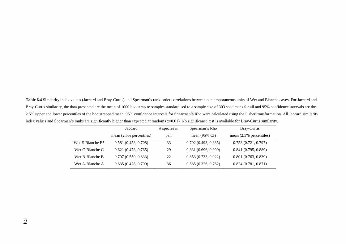
174
Table 6.4 Similarity index values (Jaccard and Bray-Curtis) and Spearman’s rank-order correlations between contemporaneous units of Wet and Blanche caves. For Jaccard and
Bray-Curtis similarity, the data presented are the mean of 1000 bootstrap re-samples standardised to a sample size of 303 specimens for all and 95% confidence intervals are the
2.5% upper and lower percentiles of the bootstrapped mean. 95% confidence intervals for Spearman’s Rho were calculated using the Fisher transformation. All Jaccard similarity
index values and Spearman’s ranks are significantly higher than expected at random (α=0.01). No significance test is available for Bray-Curtis similarity.
Jaccard
mean (2.5% percentiles)
# species in
pair
Spearman’s Rho
mean (95% CI)
Bray-Curtis
mean (2.5% percentiles)
Wet E-Blanche E* 0.581 (0.458, 0.708) 33 0.702 (0.493, 0.835) 0.758 (0.721, 0.797)
Wet C-Blanche C 0.621 (0.478, 0.765) 29 0.831 (0.696, 0.909) 0.841 (0.795, 0.889)
Wet B-Blanche B 0.707 (0.550, 0.833) 22 0.853 (0.733, 0.922) 0.801 (0.763, 0.839)
Wet A-Blanche A 0.635 (0.478, 0.790) 36 0.585 (0.326, 0.762) 0.824 (0.781, 0.871)
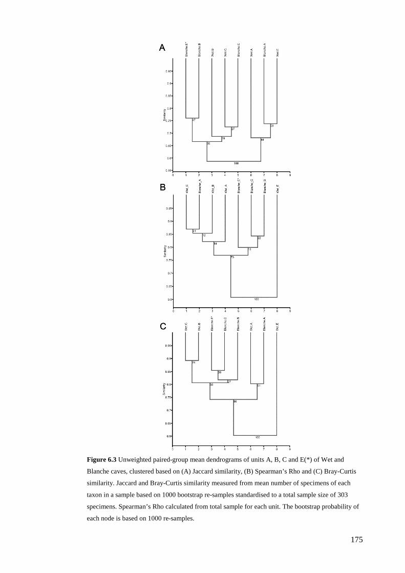
175
Figure 6.3 Unweighted paired-group mean dendrograms of units A, B, C and E(*) of Wet and
Blanche caves, clustered based on (A) Jaccard similarity, (B) Spearman’s Rho and (C) Bray-Curtis
similarity. Jaccard and Bray-Curtis similarity measured from mean number of specimens of each
taxon in a sample based on 1000 bootstrap re-samples standardised to a total sample size of 303
specimens. Spearman’s Rho calculated from total sample for each unit. The bootstrap probability of
each node is based on 1000 re-samples.
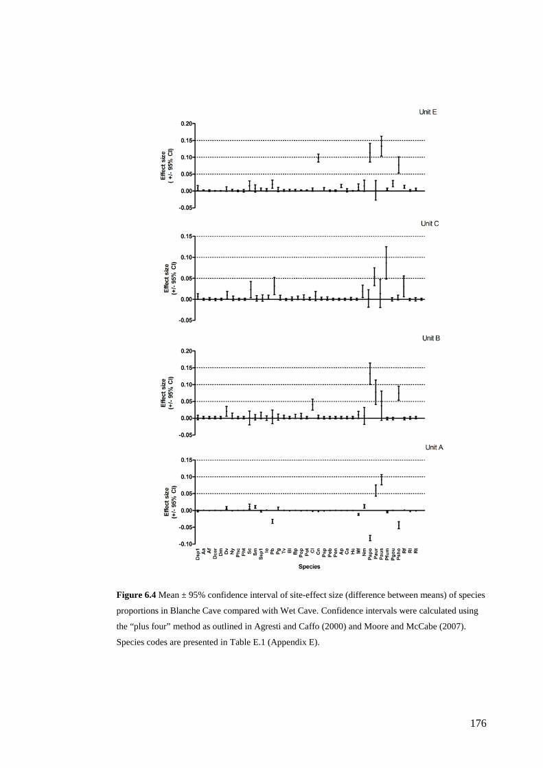
176
Figure 6.4 Mean ± 95% confidence interval of site-effect size (difference between means) of species
proportions in Blanche Cave compared with Wet Cave. Confidence intervals were calculated using
the “plus four” method as outlined in Agresti and Caffo (2000) and Moore and McCabe (2007).
Species codes are presented in Table E.1 (Appendix E).
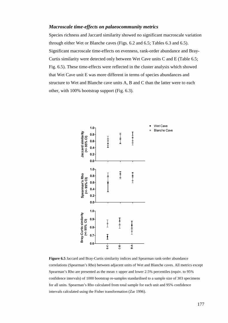
177
Macroscale time-effects on palaeocommunity metrics Species richness and Jaccard similarity showed no significant macroscale variation
through either Wet or Blanche caves (Figs. 6.2 and 6.5; Tables 6.3 and 6.5).
Significant macroscale time-effects on evenness, rank-order abundance and Bray-
Curtis similarity were detected only between Wet Cave units C and E (Table 6.5;
Fig. 6.5). These time-effects were reflected in the cluster analysis which showed
that Wet Cave unit E was more different in terms of species abundances and
structure to Wet and Blanche cave units A, B and C than the latter were to each
other, with 100% bootstrap support (Fig. 6.3).
Figure 6.5 Jaccard and Bray-Curtis similarity indices and Spearman rank-order abundance
correlations (Spearman’s Rho) between adjacent units of Wet and Blanche caves. All metrics except
Spearman’s Rho are presented as the mean ± upper and lower 2.5% percentiles (equiv. to 95%
confidence intervals) of 1000 bootstrap re-samples standardised to a sample size of 303 specimens
for all units. Spearman’s Rho calculated from total sample for each unit and 95% confidence
intervals calculated using the Fisher transformation (Zar 1996).
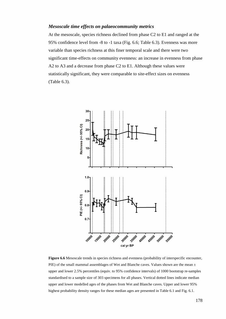
178
Mesoscale time effects on palaeocommunity metrics At the mesoscale, species richness declined from phase C2 to E1 and ranged at the
95% confidence level from -8 to -1 taxa (Fig. 6.6; Table 6.3). Evenness was more
variable than species richness at this finer temporal scale and there were two
significant time-effects on community evenness: an increase in evenness from phase
A2 to A3 and a decrease from phase C2 to E1. Although these values were
statistically significant, they were comparable to site-effect sizes on evenness
(Table 6.3).
Figure 6.6 Mesoscale trends in species richness and evenness (probability of interspecific encounter,
PIE) of the small mammal assemblages of Wet and Blanche caves. Values shown are the mean ±
upper and lower 2.5% percentiles (equiv. to 95% confidence intervals) of 1000 bootstrap re-samples
standardised to a sample size of 303 specimens for all phases. Vertical dotted lines indicate median
upper and lower modelled ages of the phases from Wet and Blanche caves. Upper and lower 95%
highest probability density ranges for these median ages are presented in Table 6.1 and Fig. 6.1.
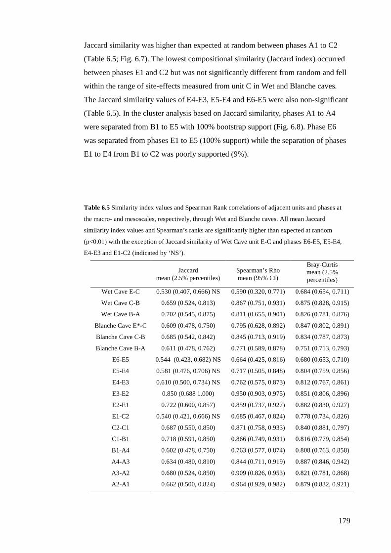
179
Jaccard similarity was higher than expected at random between phases A1 to C2
(Table 6.5; Fig. 6.7). The lowest compositional similarity (Jaccard index) occurred
between phases E1 and C2 but was not significantly different from random and fell
within the range of site-effects measured from unit C in Wet and Blanche caves.
The Jaccard similarity values of E4-E3, E5-E4 and E6-E5 were also non-significant
(Table 6.5). In the cluster analysis based on Jaccard similarity, phases A1 to A4
were separated from B1 to E5 with 100% bootstrap support (Fig. 6.8). Phase E6
was separated from phases E1 to E5 (100% support) while the separation of phases
E1 to E4 from B1 to C2 was poorly supported (9%).
Table 6.5 Similarity index values and Spearman Rank correlations of adjacent units and phases at
the macro- and mesoscales, respectively, through Wet and Blanche caves. All mean Jaccard
similarity index values and Spearman’s ranks are significantly higher than expected at random
(p<0.01) with the exception of Jaccard similarity of Wet Cave unit E-C and phases E6-E5, E5-E4,
E4-E3 and E1-C2 (indicated by ‘NS’).
Jaccard mean (2.5% percentiles)
Spearman’s Rho mean (95% CI)
Bray-Curtis mean (2.5% percentiles)
Wet Cave E-C 0.530 (0.407, 0.666) NS 0.590 (0.320, 0.771) 0.684 (0.654, 0.711)
Wet Cave C-B 0.659 (0.524, 0.813) 0.867 (0.751, 0.931) 0.875 (0.828, 0.915)
Wet Cave B-A 0.702 (0.545, 0.875) 0.811 (0.655, 0.901) 0.826 (0.781, 0.876)
Blanche Cave E*-C 0.609 (0.478, 0.750) 0.795 (0.628, 0.892) 0.847 (0.802, 0.891)
Blanche Cave C-B 0.685 (0.542, 0.842) 0.845 (0.713, 0.919) 0.834 (0.787, 0.873)
Blanche Cave B-A 0.611 (0.478, 0.762) 0.771 (0.589, 0.878) 0.751 (0.713, 0.793)
E6-E5 0.544 (0.423, 0.682) NS 0.664 (0.425, 0.816) 0.680 (0.653, 0.710)
E5-E4 0.581 (0.476, 0.706) NS 0.717 (0.505, 0.848) 0.804 (0.759, 0.856)
E4-E3 0.610 (0.500, 0.734) NS 0.762 (0.575, 0.873) 0.812 (0.767, 0.861)
E3-E2 0.850 (0.688 1.000) 0.950 (0.903, 0.975) 0.851 (0.806, 0.896)
E2-E1 0.722 (0.600, 0.857) 0.859 (0.737, 0.927) 0.882 (0.830, 0.927)
E1-C2 0.540 (0.421, 0.666) NS 0.685 (0.467, 0.824) 0.778 (0.734, 0.826)
C2-C1 0.687 (0.550, 0.850) 0.871 (0.758, 0.933) 0.840 (0.881, 0.797)
C1-B1 0.718 (0.591, 0.850) 0.866 (0.749, 0.931) 0.816 (0.779, 0.854)
B1-A4 0.602 (0.478, 0.750) 0.763 (0.577, 0.874) 0.808 (0.763, 0.858)
A4-A3 0.634 (0.480, 0.810) 0.844 (0.711, 0.919) 0.887 (0.846, 0.942)
A3-A2 0.680 (0.524, 0.850) 0.909 (0.826, 0.953) 0.821 (0.781, 0.868)
A2-A1 0.662 (0.500, 0.824) 0.964 (0.929, 0.982) 0.879 (0.832, 0.921)
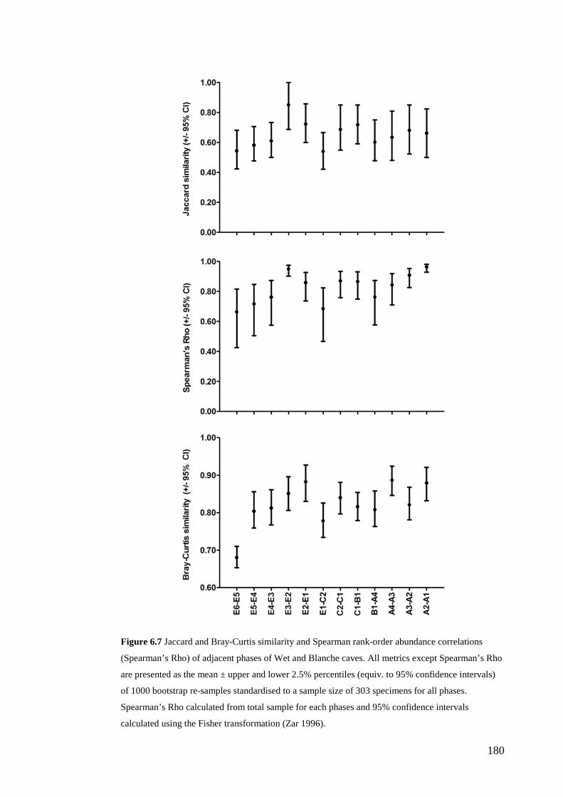
180
Figure 6.7 Jaccard and Bray-Curtis similarity and Spearman rank-order abundance correlations
(Spearman’s Rho) of adjacent phases of Wet and Blanche caves. All metrics except Spearman’s Rho
are presented as the mean ± upper and lower 2.5% percentiles (equiv. to 95% confidence intervals)
of 1000 bootstrap re-samples standardised to a sample size of 303 specimens for all phases.
Spearman’s Rho calculated from total sample for each phases and 95% confidence intervals
calculated using the Fisher transformation (Zar 1996).
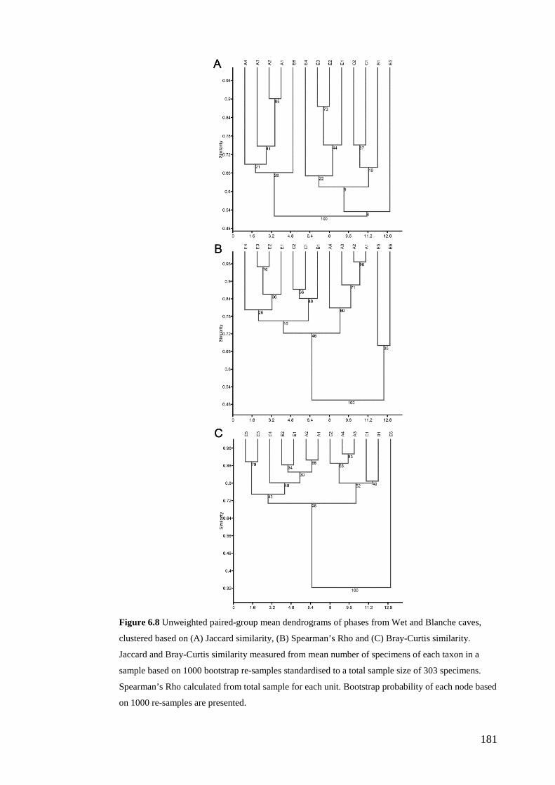
181
Figure 6.8 Unweighted paired-group mean dendrograms of phases from Wet and Blanche caves,
clustered based on (A) Jaccard similarity, (B) Spearman’s Rho and (C) Bray-Curtis similarity.
Jaccard and Bray-Curtis similarity measured from mean number of specimens of each taxon in a
sample based on 1000 bootstrap re-samples standardised to a total sample size of 303 specimens.
Spearman’s Rho calculated from total sample for each unit. Bootstrap probability of each node based
on 1000 re-samples are presented.
182
The rank-order abundance correlations of phases A1 to C2 were high and ranged
between 0.763 and 0.964 (Fig. 6.7). A decline in correlation of 0.186 occurred from
phases C2-C1 to E1-C2 (Table 6.5), reflecting a similar temporal trend as the
Jaccard similarity index (Fig. 6.7). In the cluster analysis there was only 16%
bootstrap support for the separation of phases C2 and E1 based on rank-order
abundance, contrasting with phases E5 and E6 which together were separated from
all other phases with 100% bootstrap support. The rank-order abundance correlation
of units E1 and C2 also fell within the range of the site-effect associated with unit C
for this metric (Table 6.4).
Bray-Curtis similarity was more variable at the mesoscale than Jaccard similarity
and Spearman’s Rho as reflected in the cluster analysis which identified three
separate groups (phase E6; phases A3 to C2; phases A1 to A2 and E1 to E5) with
bootstrap support of 100% and 96%, respectively (Fig. 6.8). The separation of phase
E6 from all other phases in the cluster analysis is consistent with the low Bray-
Curtis similarity measured between phases E5 and E6 (Table 6.5) and shows that
relative abundance of species in phase E6 were more different to all other phases
than would be expected at random.
Time-effects on individual species relative abundances For nearly all taxa, the magnitude of site-effects on the relative abundance of
individual species exceeded any macroscale time-effect, severely limiting the extent
to which temporal variation in relative species abundances within individual sites
could be examined (Tables E.2–E.5 Appendix E). In addition, significant
macroscale linear trends in relative abundance were detected for only c. 35% of the
Blanche Cave taxa which occurred in three or more units (Table E.6 Appendix E).
Wet Cave provided more reliable estimates of macroscale trends in species
proportions, with 57% of taxa demonstrating significant linear trends in this site
(Table E.6 Appendix E). Only five species had significant linear trends in both
assemblages (Sminthopsis murina, Perameles gunnii, Notomys mitchellii,
Pseudomys auritus and Pseudomys australis), and in all cases, the patterns of
variation with time were similar, despite significant differences in relative
abundance values between the two sites for some units (Fig. 6.9; Table E.6).

183
In addition to the five species which demonstrated significant and similar trends in
abundance through the Wet and Blanche Cave sequences at the macroscale,
significant linear trends at this temporal resolution were detected for a further 10
species which occurred in at least three units of one of the two sites (Fig. 6.10).
Significant linear trends at the mesoscale were demonstrated by 15 of 32 species
identified from four or more phases (Table E.7 Appendix E; Fig. 6.11).
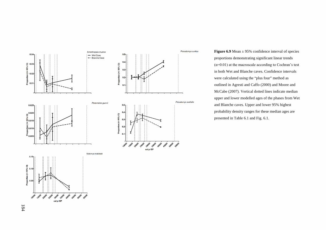
184
Figure 6.9 Mean ± 95% confidence interval of species
proportions demonstrating significant linear trends
(α=0.01) at the macroscale according to Cochran’s test
in both Wet and Blanche caves. Confidence intervals
were calculated using the “plus four” method as
outlined in Agresti and Caffo (2000) and Moore and
McCabe (2007). Vertical dotted lines indicate median
upper and lower modelled ages of the phases from Wet
and Blanche caves. Upper and lower 95% highest
probability density ranges for these median ages are
presented in Table 6.1 and Fig. 6.1.
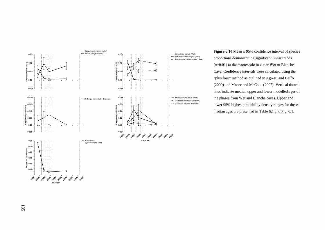
185
Figure 6.10 Mean ± 95% confidence interval of species
proportions demonstrating significant linear trends
(α=0.01) at the macroscale in either Wet or Blanche
Cave. Confidence intervals were calculated using the
“plus four” method as outlined in Agresti and Caffo
(2000) and Moore and McCabe (2007). Vertical dotted
lines indicate median upper and lower modelled ages of
the phases from Wet and Blanche caves. Upper and
lower 95% highest probability density ranges for these
median ages are presented in Table 6.1 and Fig. 6.1.
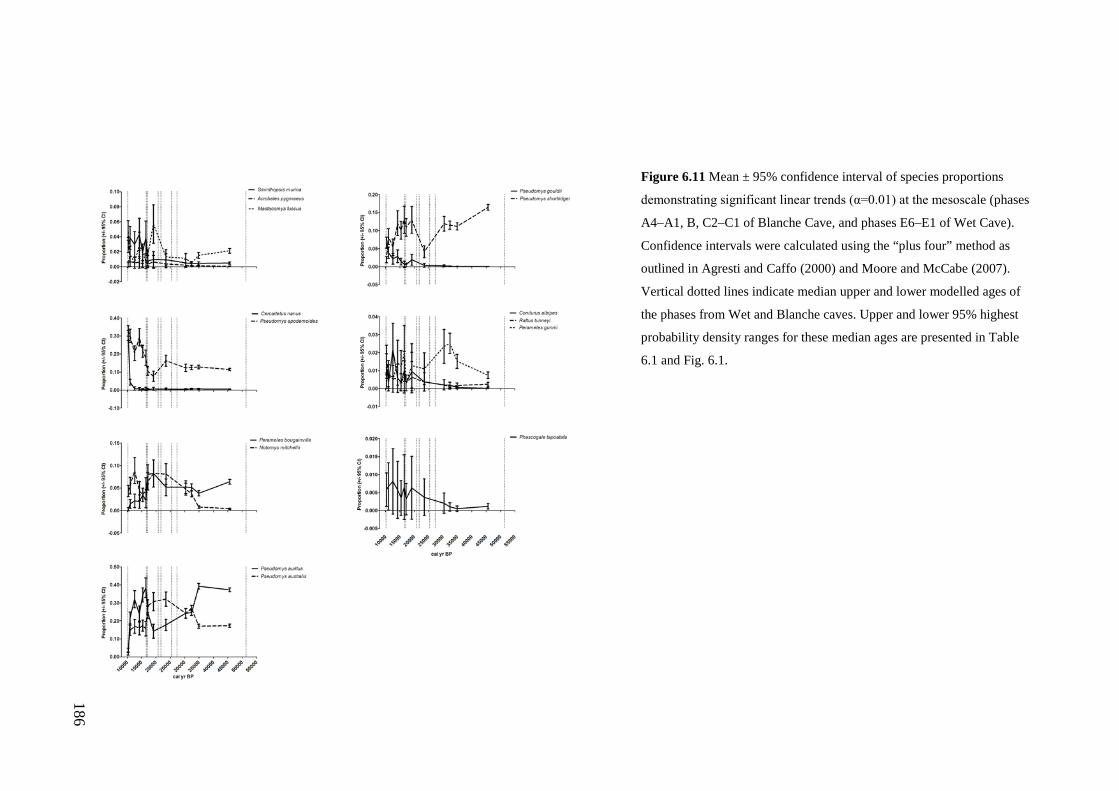
186
Figure 6.11 Mean ± 95% confidence interval of species proportions
demonstrating significant linear trends (α=0.01) at the mesoscale (phases
A4–A1, B, C2–C1 of Blanche Cave, and phases E6–E1 of Wet Cave).
Confidence intervals were calculated using the “plus four” method as
outlined in Agresti and Caffo (2000) and Moore and McCabe (2007).
Vertical dotted lines indicate median upper and lower modelled ages of
the phases from Wet and Blanche caves. Upper and lower 95% highest
probability density ranges for these median ages are presented in Table
6.1 and Fig. 6.1.
187
Discussion
Similarity of Wet and Blanche Cave fossil assemblages: palaeocommunity
variables The lack of statistically significant site-effects on species richness, composition and
abundance ranks, and high Bray-Curtis index values of the assemblages from Wet
and Blanche caves shows that overall, the two sites provided similar
palaeocommunity samples for each time period represented by units A, B, C and
E(*). This demonstrated similarity is consistent with expectations based on their
spatial proximity, similar temporal span and accumulation-mode (tytonid owls;
Macken and Reed 2013; Macken et al. 2013b). By comparison, significant
differences in assemblage evenness and the relative abundances of individual
species between the sites revealed sampling effects not evident in the metrics based
on species presence/absence and rank-order data.
Quantifying variability in local palaeocommunities is critical for testing patterns of
stasis and/or change in palaeocommunities across space and time (Bennington and
Bambach 1996). Thus, the similarity of palaeocommunity variables measured from
the assemblages of units A, B and C of Wet and Blanche caves suggests that any
temporal variability and/or stability observed in these metrics reflects real patterns
with time at the macroscale.
We note that the similarity of whole-assemblage variables measured directly
between Wet Cave unit E and Blanche Cave unit E* is surprising given that they are
not temporally equivalent (unit E* overlaps, but does not cover the entire temporal
period represented in Wet Cave unit E; Table 6.1; Macken et al. 2013b). One reason
for the similarity between these units may be the mixing of bone material of
Pleistocene and Holocene ages in unit E*. As shown by St Pierre et al. (2012),
Holocene aged speleothem (calcium carbonate) straws and charcoal are present in
Blanche Cave layers 1 and 3 which correspond to unit E* (Table E.1 Appendix E).
However, Pleistocene aged charcoal samples are also present in layers 1 to 3. The
mixed age of materials in these layers suggests that reworking occurred during or
following deposition. Site disturbance by human activity is the likely cause of such
mixing in the upper layers of the Blanche Cave deposit as the site has a long history
of visitation by European settlers in the region. In particular, guano collection in
188
Blanche Cave may have stripped the younger Holocene aged sediments from the
study site, resulting in disturbance to the Pleistocene aged layers that are today
represented by the top layers of the deposit (Darrénougué et al. 2009).
Alternatively, layers 1 to 3 may be Holocene aged and contaminated with
Pleistocene aged material as a result of the site disturbance. Further dating of
materials from the upper layers in Blanche Cave is required to understand the full
extent and nature of reworking that may have occurred over the history of the site.
However, regardless of the specific processes involved, the mixed age of sediments,
and potentially of fossil material in unit E*, may have increased the time-averaging
of fossil faunas in this section of Blanche Cave. Such mixing of faunas of different
ages can inflate species richness by increasing the likelihood of sampling rare fauna
(Hadly 1999), and/or by the consolidation of faunas from separate environmental
and climatic periods (Graham 1985). This greater time-averaging of the unit E*
faunas may account for the apparent similarity in whole-assemblage attributes
between this assemblage and that from Wet Cave unit E.
We also note that there are differences in the magnitude and significance of time-
effects between units E and C of Wet Cave and units E* and C of Blanche Cave.
This variation reveals sampling effects not captured by the alpha or beta diversity
metrics measured as site-effects alone. For example, divergence in the temporal
trends associated with units E and E* is evident in the cluster analyses, where units
E and E* are relatively more different to each other than units A, B and C. Of
particular note is Bray-Curtis similarity which shows that the relative abundances of
species from Wet Cave units C to E are more different than from Blanche Cave unit
C and E*, consistent with expectations based on the known temporal-inequality of
units E and E* (Table 6.5). Given the sampling limitations of Blanche Cave unit E*,
we do not provide any further evaluation of temporal trends between units C and E*
from this site.
Similarity of Wet and Blanche Cave fossil assemblages: relative abundance
of individual species While the palaeocommunity variables are similar between Wet and Blanche caves,
the relative abundances of individual species varied between contemporaneous
units. This is not surprising given the diverse range of processes involved in fossil
189
accumulation and which can contribute to spatial heterogeneity in fossil occurrences
within and among sites. Differences in the relative abundances of species between
contemporaneous units in Wet and Blanche caves are consistent with other studies
that have found that fossil specimens are not evenly distributed across a single
sedimentary horizon or across suitable habitat patches in living communities (e.g.,
Brown et al. 1995). For example, Bennington and Bambach (1996) found that
replicate samples of fossil molluscs and brachiopods from marine shales had
different underlying species abundance distributions, suggesting that time-averaging
in the shales was not long enough to reduce spatial variability in the relative
abundances of species within an assemblage. This heterogeneity may result from
patchiness in the living community, taphonomic processes and/or sampling error.
In the case of Wet and Blanche caves, taphonomic processes and sampling error are
expected to account for the site-based differences observed, rather than patchiness
in the living community. While it is expected that individuals of populations would
have been patchily distributed in the Pleistocene landscape around the caves, such
patchiness would have had a limited effect on the distribution of the relative
abundances of species in the assemblages given the sampling mode (transport of
animal remains to the caves by owls).
The influences of other biases such as variation in bone and/or teeth preservation
are commonly observed in fossil assemblages (e.g., Fernandez-Jalvo and Andrews
1992). To address these taphonomic concerns, Bobe et al. (2002) compared the
percentage occurrence of different skeletal-elements against taxonomic variability
through time to establish the extent to which changes in the abundances of species
may have been caused by taphonomic and/or ecological processes. Such an
approach was not suitable for the assemblages from Wet and Blanche caves where,
given the density of bone material, only cranio-dental specimens were identified.
Additionally, the bias towards small mammals throughout both sequences shows
that the primary taphonomic filter (tytonid owls) remained similar through the last
glacial cycle, when both the whole assemblage, including mammals with body mass
>2.5 kg (McDowell 2001; Laslett 2006) and only the small mammal component
(Fig E.3 Appendix E) are considered.
190
The Cochran-Armitage tests and relative magnitude of site- and time-effects show
that, for the majority of species, temporal trends in the relative abundances of
individual species could not be used to establish the stability or otherwise of species
populations through time. This lack of confidence in the relative abundance trends
arises both as a result of the sampling variance between the two sites and inadequate
sample sizes between consecutive units within single sites. However, of particular
note is that for those species where significant temporal trends were detected in
both sites, the trends were the same or very similar (Fig. 6.3). These results suggest
that where sampling was adequate, trends in species proportions were preserved in
the same way in the two deposits, regardless of the sampling variation between
them. This suggests that such trends are biologically significant.
Macro- versus mesoscale patterns of natural variation, persistence and
intrinsic thresholds of change To assess the ecological significance of temporal change observed in ecological
variables measured from the assemblages of Wet and Blanche caves, we integrated
the numeric hierarchy of Rahel (1990) and terminology of Bennington and
Bambach (1996; Table 6.2). According to Bennington and Bambach (1996), after
site-effects are accounted for, if two samples have statistically different species
abundance distributions, they may be assumed to have come from different
palaeocommunity types (Table 6.2). However, as noted by Rahel (1990), the
relative abundances of species within a community may be highly variable with
time while other variables such as rank-order abundance and composition remain
unchanged. Further, Hadly and Barnosky (2009) suggested that while changes in
the relative abundances of species are the “early warning signal” of environmental
impacts on species (p. 47), they also argued that changes in relative abundance
alone do not constitute significant change from a normal baseline of variation
operating at the species level within a palaeocommunity. Rather, based on evidence
from fossil and modern assemblages, they suggested that variation in the relative
abundances of species is the normal type of response to climate change and other
disturbances across different temporal scales.
Given these perspectives and the observation that relative abundances were poorly
sampled in the Wet and Blanche caves, we used the more conservative ecological
191
variable of rank-order abundance to assess the stability of the palaeocommunity
through last glacial cycle. This metric lies in the middle of Rahel’s (1990)
hierarchy. An ecological driver of stability in abundance ranks may be synchrony of
changes in the relative abundance of species within a community in response to
disturbance. This may reflect similar responses of individual species to
environmental or climatic changes (Rahel, 1990). However, individualistic
responses of populations (species) to climate change are more common and lead to
composite effects on communities (Stewart 2008). Of particular interest then was
whether the relative abundance of species through the last glacial cycle varied
individually and beyond thresholds operating within the palaeocommunity to lead to
a new rank-order abundance structure, and hence, a new palaeocommunity type?
In taking this approach, we acknowledge that Bennington and Bambach (1996)
cautioned against the use of non-parametric analysis of rank-order abundances.
They argued that even small differences in the NISP values of species between
samples makes them susceptible to accepting the null hypothesis (ρ=0, no
association between samples) when there is, in fact, an association or correlation of
species ranks between them. However, Spearman’s Rho is commonly used in the
analysis of fossil assemblages, particularly to assess the fidelity of live-dead
assemblages (e.g., Kidwell 2001; Terry 2010a, b). It has also been used in
ecological studies (e.g., Rabonsky et al. 2011) and has been suggested as a useful
measure for detecting early signs of change in ecological assemblages (Magurran
and Henderson 2010). Further, the alternative parametric ANOVA suggested by
Bennington and Bambach (1996) was not suitable for the present study as only a
limited number of replicates was available for the macroscale analysis (n=2), while
only single samples were available for each phase at the mesoscale.
This lack of sample replication is common in the study of vertebrate fossil
assemblages, where sample(s) are collected from quadrats or grids non-randomly
positioned within a depositional environment (e.g., river channel or cave floor), as
was the case for Wet and Blanche caves. Despite the collection of samples from
multiple quadrats in some vertebrate studies, they are rarely treated as independent
replicates as (a) specimens from different quadrats may have come from the same
individual, (b) samples from nearby quadrats are commonly pooled to increase
192
sample size until additional sampling effort is unlikely to recover new taxa
(“sampling to redundancy”; Lyman 2008, p. 143), and (3) there is often a limited
capacity to temporally correlate specimens between sites due to varying
depositional histories, temporal coverage and time-averaging. These and other
sampling issues and strategies associated with vertebrate fossil assemblages are
discussed in more detail elsewhere (e.g., Lyman 2008; Terry 2009).
Palaeocommunity reorganisation
Within the range of sampling variation observed between Wet and Blanche caves,
the macro- and mesoscale analyses suggest that a single palaeocommunity type
persisted from 51.4 to 17.1 kyr BP (95% CI: 60.0 to 16.7 kyr BP). This stability is
observed despite evidence for significant temporal variation (based on 95% CI and
time-effect > site-effect) in the relative abundances of some taxa over this time. By
comparison, the low rank-order abundance correlation of units C and E in Wet Cave
and separation of these units in the cluster analysis based on this variable with
100% bootstrap support suggests that the palaeocommunities from these two time
periods may be significantly different.
Palaeocommunity reorganisation between these units is reflected at the mesoscale in
the significant decline in species richness from phase C2 to E1. Species richness
does not appear in Rahel’s (1990) hierarchy but reflects community-level variation
at a scale consistent with composition as both of these metrics are based on species
presence/absence data. The variation in the presence of individual species within the
palaeocommunity likely reflects the dispersal of species from the region proximal to
the caves during phase E1, rather than local extinction: species absent from phase
E1 return to the Wet Cave record in one of phases E2 to E6 or the Holocene
samples of Robertson Cave entrance chamber (pers. obs.). Only one species may
have gone locally extinct over the transition of phase C2 to E1 (Bettongia gaimardi)
as this species is not known from younger fossil assemblages of the Naracoorte
Caves. Thus, despite our lack of confidence in the trends observed in the relative
abundances of individual species, the significant decline in species richness from
phase C2 to E1 reflects re-organisation of the palaeocommunity and the emergence,
at least during phase E1, of a new palaeocommunity type from that of the previous
c. 33 kyrs. We also note that the mean decline in species richness of five (based on
193
the sample-size standardised data; 95% CI: 1 to 8) from phase C2 to E1 is the same
as the decline in species richness of a small mammal assemblage over the
Pleistocene–Holocene transition in Samwell Cave, northern California (Blois et al.
2010). The loss of species observed in the Samwell Cave sequence at the end of the
Pleistocene was coincident with a decline of c. 0.15 in Jaccard similarity and c. 0.06
in Bray-Curtis similarity. These changes were interpreted as reflecting a
reorganisation of the palaeocommunity at the end of the Pleistocene (Blois et al.
2010). As the values measured from Samwell Cave are almost identical to the
differences between these metrics observed in the assemblages from Wet and
Blanche caves from phase C2 to E1, we interpret a similar degree of
palaeocommunity reorganisation in the Naracoorte small mammal faunas following
the last glacial maximum.
Interestingly, the high and statistically significant compositional similarity and
rank-order abundance correlation of phases E1 and E2, and phases E2 and E3
suggest a period of relative stability in the palaeocommunity from c. 16.7 to 14.0
kyr BP (95% CI: 17.1 to 12.7). This is followed by a possible second reorganisation
of the palaeocommunity from phase E5 to E6, 10.8 and 10.5 kyr BP (95% CI: 11.2
to 10.9 kyr BP). The evidence for this second reorganisation is the low mean rank-
order abundance correlation of these phases when compared with the other phases;
although unlike the first significant episode of palaeocommunity change, the second
is not associated with a significant change in species richness.
Palaeoclimatic and environmental thresholds It is common for palaeoenvironmental reconstructions to be based on the
contemporary distribution and niche space of the species identified in a fossil
assemblage. Such properties are then used to infer the local extrinsic and intrinsic
factors associated with a palaeocommunity at the time of accumulation. However,
geographic range and niche contraction as a result of human mediated landscape
change is expected to severely limit the accuracy of palaeoenvironmental
reconstructions using this technique (e.g., Belyea 2007; Bilney et al. 2010).
Consequently, we are cautious in inferring the environmental, climatic and
biological correlates of the small mammal palaeocommunities from the fauna
194
themselves and instead contrast them against independent records of palaeoclimatic
and environmental conditions (Fig. 6.12).
As we have only used a narrow range of palaeoclimatic and environmental records,
we acknowledge that they may not best explain the palaeocommunity changes
observed in the Naracoorte record. The palaeoclimatic and environmental data
presented and discussed here were selected on the basis of their proximity to the
Naracoorte Caves, temporal coverage and chronological resolution. As such, while
they provide a reference to local and regional temperature, effective precipitation
and vegetation using a range of proxies, they do not cover all the extrinsic factors
that are expected to interact together to drive palaeocommunity variability through
time. For example, as examined by Broughton et al. (2008), increased seasonality
may be more closely related to changes in vertebrate palaeocommunities through
species competitive processes, preceding impacts related to temperature thresholds.
However, at the present time there are no proxy data for seasonality available for
late Quaternary south-eastern South Australia, limiting us to the palaeoclimatic and
environmental data presented in Figure 6.12.
Macroscale trends in SST, vegetation types and speleothem growth phases show
that palaeoclimatic and environmental conditions were variable through MIS-3 and
MIS-2 (c. 51.4 to 17.1 kyr BP). The early glacial periods of MIS-3 and MIS-2 are
characterised by two periods of high effective moisture availability (Ayliffe et al.
1998) and a trend towards lower mean SSTs (although, fine resolution SST data
show high variability through units A, B and C; Fig. 6.12; Lopes dos Santos et al.
2012). The temporal variability in effective precipitation demonstrated in these
records is also reflected in the sedimentary records of lakes in south-eastern South
Australia and south-western Victoria (Dodson 1975; Dodson 1977; Cook 2009).
During the early glacial period, lacustral phases in the Murray Darling Basin and
palaeochannels that fed the Willandra lakes systems in south-eastern Australia were
characterised by periods of large, high energy flows and high lake levels, driven by
winter snowmelts from the Snowy Mountains (Bowler et al. 2007; Bowler et al.
2012). Palaeoclimate records reflect the influence of seasonal processes on
deposition in these environments (Kemp and Spooner 2007; Macken et al. 2013a;
195
Petherick et al. 2013). By comparison, if there were changes in local or regional
effective precipitation and/or seasonality, they had minimal impact on the sediment
type and deposition of sediments forming unit A in Wet and Blanche caves over the
later stages of MIS-3 (Macken et al. 2013a).
The pollen data from Blanche Cave reveal a trend towards increasing relative
abundance of woody taxa (e.g., Eucalyptus, Casuarina, Acacia and Banksia) at the
expense of herbaceous (e.g., Poaceae) and woody-herbaceous taxa (e.g.,
Asteraceae) from units A to B. A more dramatic change in vegetation-types is
evident from unit B to C, with a decline in the relative abundance of woody taxa by
c. 25%, while herbaceous taxa increased by c. 10% and woody-herbaceous by c.
15% (N.B., The genera listed for each of the vegetation groupings was sourced from
D’Costa and Kershaw (1997)). Pollen records examined from lakes Bolac and
Turungmoroke in south-western Victoria reflect a similar trend of vegetation
community change, where open-grassland steppe encroached upon woodlands
towards the end of MIS-3 and into MIS-2 (Cook 2009). Shifts towards open
grasslands over the LGM are exhibited in a number of pollen cores across Australia
(Turney et al. 2006; Petherick et al. 2013); although, Petherick et al. (2013) noted
sites in south-east Queensland and northern NSW that exhibit higher percentages of
Casuarinaceae than those from southern Australia at the time of the LGM. They
also noted the Lake Surprise record of south-western Victoria which recorded a
peak in Eucalyptus over the LGM (Builth et al. 2008).
Given the variation in pollen signals from across these sites and the limited
resolution of pollen data currently published from Blanche Cave, the timing of
vegetation changes associated with the last glacial cycle from the Naracoorte region
is difficult to interpret. The shift from a positive to negative moisture budget at c. 20
kyr BP reflected in the speleothem record (Ayliffe et al. 1998) and/or the rapid
increase in SST over the accumulation of unit C from c. 18.7 kyr BP (Lopes dos
Santos et al. 2012) may have contributed to the apparent changes in the dominant
vegetation types in the Blanche Cave pollen record observed from unit B to unit C.
Finer temporal scale pollen analysis using the distinct pollen groupings (rather than
broad vegetation types) is required to temporally constrain the vegetation changes
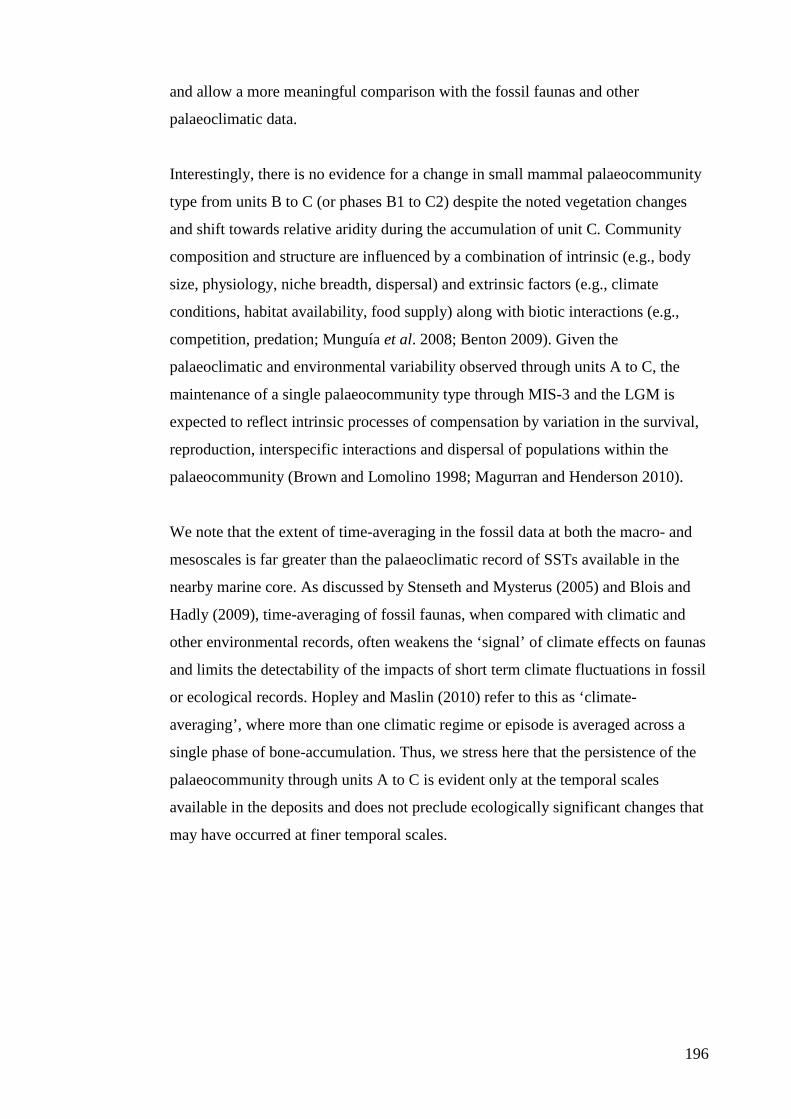
196
and allow a more meaningful comparison with the fossil faunas and other
palaeoclimatic data.
Interestingly, there is no evidence for a change in small mammal palaeocommunity
type from units B to C (or phases B1 to C2) despite the noted vegetation changes
and shift towards relative aridity during the accumulation of unit C. Community
composition and structure are influenced by a combination of intrinsic (e.g., body
size, physiology, niche breadth, dispersal) and extrinsic factors (e.g., climate
conditions, habitat availability, food supply) along with biotic interactions (e.g.,
competition, predation; Munguía et al. 2008; Benton 2009). Given the
palaeoclimatic and environmental variability observed through units A to C, the
maintenance of a single palaeocommunity type through MIS-3 and the LGM is
expected to reflect intrinsic processes of compensation by variation in the survival,
reproduction, interspecific interactions and dispersal of populations within the
palaeocommunity (Brown and Lomolino 1998; Magurran and Henderson 2010).
We note that the extent of time-averaging in the fossil data at both the macro- and
mesoscales is far greater than the palaeoclimatic record of SSTs available in the
nearby marine core. As discussed by Stenseth and Mysterus (2005) and Blois and
Hadly (2009), time-averaging of fossil faunas, when compared with climatic and
other environmental records, often weakens the ‘signal’ of climate effects on faunas
and limits the detectability of the impacts of short term climate fluctuations in fossil
or ecological records. Hopley and Maslin (2010) refer to this as ‘climate-
averaging’, where more than one climatic regime or episode is averaged across a
single phase of bone-accumulation. Thus, we stress here that the persistence of the
palaeocommunity through units A to C is evident only at the temporal scales
available in the deposits and does not preclude ecologically significant changes that
may have occurred at finer temporal scales.
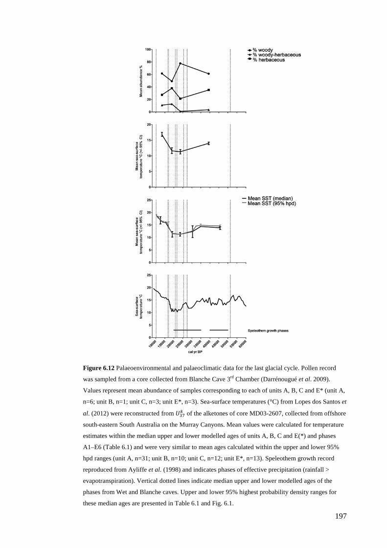
197
Figure 6.12 Palaeoenvironmental and palaeoclimatic data for the last glacial cycle. Pollen record
was sampled from a core collected from Blanche Cave 3rd Chamber (Darrénougué et al. 2009).
Values represent mean abundance of samples corresponding to each of units A, B, C and E* (unit A,
n=6; unit B, n=1; unit C, n=3; unit E*, n=3). Sea-surface temperatures (°C) from Lopes dos Santos et
al. (2012) were reconstructed from 𝑈37𝑘 of the alketones of core MD03-2607, collected from offshore
south-eastern South Australia on the Murray Canyons. Mean values were calculated for temperature
estimates within the median upper and lower modelled ages of units A, B, C and E(*) and phases
A1–E6 (Table 6.1) and were very similar to mean ages calculated within the upper and lower 95%
hpd ranges (unit A, n=31; unit B, n=10; unit C, n=12; unit E*, n=13). Speleothem growth record
reproduced from Ayliffe et al. (1998) and indicates phases of effective precipitation (rainfall >
evapotranspiration). Vertical dotted lines indicate median upper and lower modelled ages of the
phases from Wet and Blanche caves. Upper and lower 95% highest probability density ranges for
these median ages are presented in Table 6.1 and Fig. 6.1.
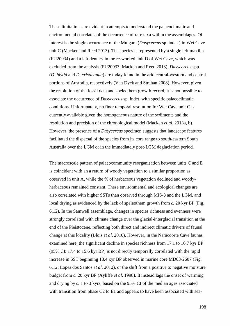
198
These limitations are evident in attempts to understand the palaeoclimatic and
environmental correlates of the occurrence of rare taxa within the assemblages. Of
interest is the single occurrence of the Mulgara (Dasycercus sp. indet.) in Wet Cave
unit C (Macken and Reed 2013). The species is represented by a single left maxilla
(FU20934) and a left dentary in the re-worked unit D of Wet Cave, which was
excluded from the analysis (FU20933; Macken and Reed 2013). Dasycercus spp.
(D. blythi and D. cristicauda) are today found in the arid central-western and central
portions of Australia, respectively (Van Dyck and Strahan 2008). However, given
the resolution of the fossil data and speleothem growth record, it is not possible to
associate the occurrence of Dasycercus sp. indet. with specific palaeoclimatic
conditions. Unfortunately, no finer temporal resolution for Wet Cave unit C is
currently available given the homogeneous nature of the sediments and the
resolution and precision of the chronological model (Macken et al. 2013a, b).
However, the presence of a Dasycercus specimen suggests that landscape features
facilitated the dispersal of the species from its core range to south-eastern South
Australia over the LGM or in the immediately post-LGM deglaciation period.
The macroscale pattern of palaeocommunity reorganisation between units C and E
is coincident with an a return of woody vegetation to a similar proportion as
observed in unit A, while the % of herbaceous vegetation declined and woody-
herbaceous remained constant. These environmental and ecological changes are
also correlated with higher SSTs than observed through MIS-3 and the LGM, and
local drying as evidenced by the lack of speleothem growth from c. 20 kyr BP (Fig.
6.12). In the Samwell assemblage, changes in species richness and evenness were
strongly correlated with climate change over the glacial-interglacial transition at the
end of the Pleistocene, reflecting both direct and indirect climatic drivers of faunal
change at this locality (Blois et al. 2010). However, in the Naracoorte Cave faunas
examined here, the significant decline in species richness from 17.1 to 16.7 kyr BP
(95% CI: 17.4 to 15.6 kyr BP) is not directly temporally correlated with the rapid
increase in SST beginning 18.4 kyr BP observed in marine core MD03-2607 (Fig.
6.12; Lopes dos Santos et al. 2012), or the shift from a positive to negative moisture
budget from c. 20 kyr BP (Ayliffe et al. 1998). It instead lags the onset of warming
and drying by c. 1 to 3 kyrs, based on the 95% CI of the median ages associated
with transition from phase C2 to E1 and appears to have been associated with sea-
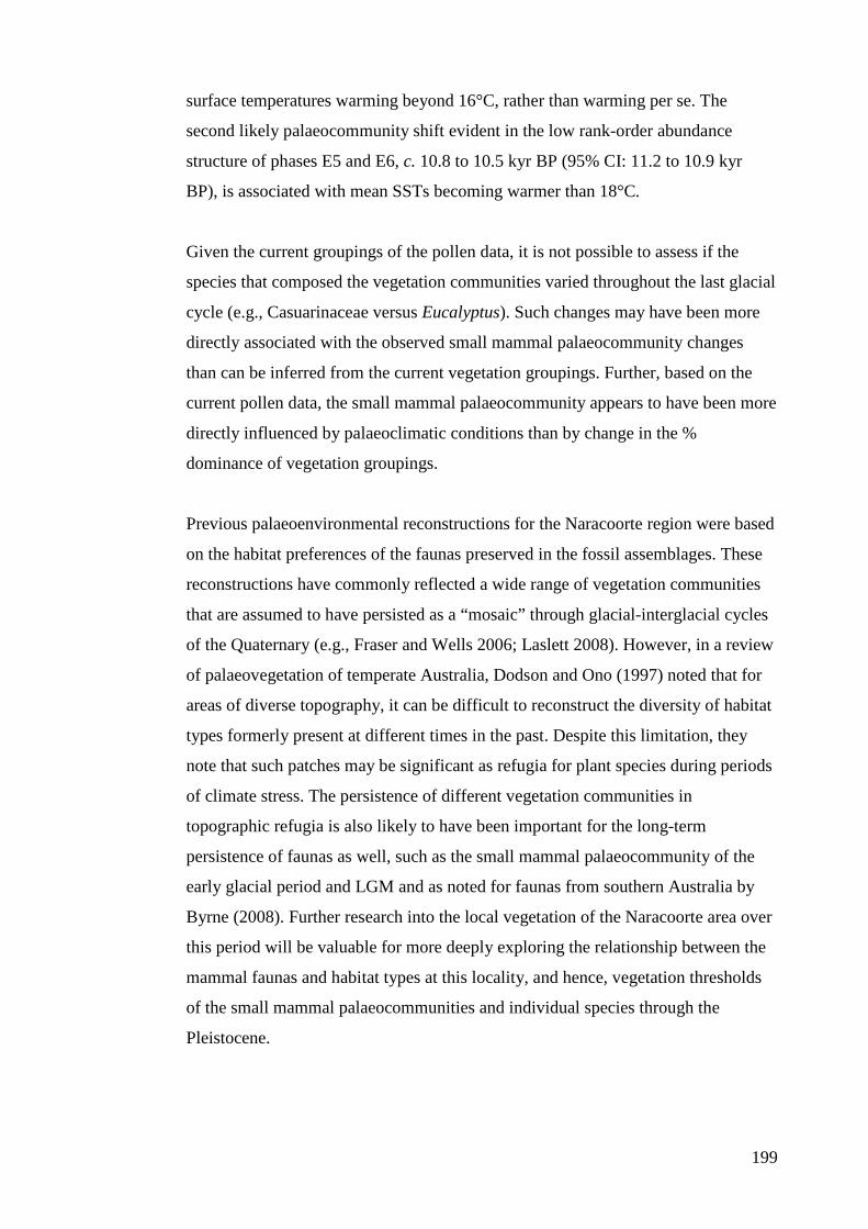
199
surface temperatures warming beyond 16°C, rather than warming per se. The
second likely palaeocommunity shift evident in the low rank-order abundance
structure of phases E5 and E6, c. 10.8 to 10.5 kyr BP (95% CI: 11.2 to 10.9 kyr
BP), is associated with mean SSTs becoming warmer than 18°C.
Given the current groupings of the pollen data, it is not possible to assess if the
species that composed the vegetation communities varied throughout the last glacial
cycle (e.g., Casuarinaceae versus Eucalyptus). Such changes may have been more
directly associated with the observed small mammal palaeocommunity changes
than can be inferred from the current vegetation groupings. Further, based on the
current pollen data, the small mammal palaeocommunity appears to have been more
directly influenced by palaeoclimatic conditions than by change in the %
dominance of vegetation groupings.
Previous palaeoenvironmental reconstructions for the Naracoorte region were based
on the habitat preferences of the faunas preserved in the fossil assemblages. These
reconstructions have commonly reflected a wide range of vegetation communities
that are assumed to have persisted as a “mosaic” through glacial-interglacial cycles
of the Quaternary (e.g., Fraser and Wells 2006; Laslett 2008). However, in a review
of palaeovegetation of temperate Australia, Dodson and Ono (1997) noted that for
areas of diverse topography, it can be difficult to reconstruct the diversity of habitat
types formerly present at different times in the past. Despite this limitation, they
note that such patches may be significant as refugia for plant species during periods
of climate stress. The persistence of different vegetation communities in
topographic refugia is also likely to have been important for the long-term
persistence of faunas as well, such as the small mammal palaeocommunity of the
early glacial period and LGM and as noted for faunas from southern Australia by
Byrne (2008). Further research into the local vegetation of the Naracoorte area over
this period will be valuable for more deeply exploring the relationship between the
mammal faunas and habitat types at this locality, and hence, vegetation thresholds
of the small mammal palaeocommunities and individual species through the
Pleistocene.
200
Conclusions The detection of ecologically significant variation in the assemblages from Wet and
Blanche caves was dependent upon both the temporal and ecological scale of
observation. When contrasted against other palaeocommunity records where whole-
scale faunal turnover resulted in compositionally dissimilar assemblages (e.g.,
Hocknull et al. 2007), the small mammal palaeocommunity of late Quaternary
Naracoorte appears to have been highly stable and persistent. However, using a
nested numeric hierarchy revealed temporal variation across ecological variables of
the fossil assemblages, with at least one episode of significant palaeocommunity
reorganisation over the post-LGM deglaciation.
Palaeocommunity reorganisation occurred at 17.1 to 16.7 kyr BP, 1–3 kyr after the
commencement of post-glacial warming from 18.4 kyr BP and local drying from c.
20 kyr BP. This palaeocommunity shift was correlated with SSTs warming beyond
16°C and dry conditions when compared with the previous c. 33 kyr BP. A likely
second palaeocommunity reorganisation event was recorded at 10.8 to 10.5 kyr BP,
correlated with SSTs warming past 18°C and continued relative aridity. These
patterns provide some insight into the likely extrinsic thresholds for the successive
palaeocommunities of the Naracoorte region through the last glacial cycle.
However, further research is required to reveal the relationships between the small
mammal fauna, local vegetation and habitat characteristics that are expected to have
exerted strong controls on the survival, reproduction, interspecific interactions and
dispersal of populations across the region.
Whole community-level variables measured from the assemblages of Wet and
Blanche caves were highly consistent between the two sites for temporally
equivalent units. This limited site-based sampling variation provided a robust and
reliable record of whole-palaeocommunity change with time. By comparison, our
analysis showed that the relative abundances of individual species in the deposits
were affected by sampling variation and the patchy distribution of specimens across
bedding plains or stratigraphic horizons. These observations cautioned against using
changes in the relative abundance of individual species to infer individual species
responses to climate change. However, where the relative abundances of individual
species were adequately and consistently sampled in the two sites, there was
201
evidence for large magnitude changes in the abundances of some species, while
others persisted at low abundance for the majority of the record.
Ecological thresholds operating within the palaeocommunity maintained the rank-
order abundance distribution of species within the palaeocommunity, despite
evidence for variation in the relative abundances of some species and
palaeoclimatic and vegetation change through the early glacial period and LGM
from 51.7 to 17.1 kyr BP. We suggest that change in the abundances of species
reflects intrinsic and community level processes in response to climatic and
environmental change and were within thresholds that maintained the
palaeocommunity type through this time.
The Wet and Blanche cave records also reflect the ability of the palaeocommunity
to recover species following a severe disruption. This may be related to an inherent
ability of the broader ecosystem to resist or recover from disturbance. For example,
connectivity of habitats and suitable patches, which are today observed to be critical
factors in species dispersal and migration, was likely a feature of the south-eastern
South Australia ecosystem through the last glacial cycle.
From a biodiversity conservation perspective, the long-term records from Wet and
Blanche caves strengthen arguments for a focus on the interaction of intrinsic and
extrinsic thresholds operating on communities and individual species across
multiple scales (du Toit 2010). Unfortunately, the majority of the small mammals
that formed the successive palaeocommunity types through the last glacial cycle are
no longer present in south-eastern South Australia today (Robinson et al. 2000).
However, the Naracoorte record reveals a remarkable capacity for some species to
persist either at very low abundance, or to maintain populations despite severe
increases and decreases in population size and/or density, in response to
opportunities within the community and/or environment across different time
scales.
Acknowledgments We thank Dr Jessica Blois who generously provided a copy of a bootstrap
resampling R script and Mr Pawel Skuza for advice on the statistical analyses. We

202
also thank Drs Raquel Lopes dos Santos and Patrick De Deckker who kindly
provided raw SST data from marine core MD03-2607 for reproduction. We are also
grateful for the feedback from Dr Trevor Worthy on an earlier version of the
manuscript. Funding for the Naracoorte Cave research was provided via the
Australian Government’s Caring for our Country initiative (Grant OC11-00487).
203
7. Concluding Discussion The motivating questions for this thesis were drawn from a wide range of ecological
literature and relate to knowledge gaps that hamper conservation efforts,
particularly those associated with climate change. These questions were:
(a) How do ecosystems respond in the short and long-term to disturbance,
(b) What is the natural range of variation exhibited by ecosystems at
different temporal and spatial scales, and
(c) What are the limits of resilience, or thresholds beyond which ecosystems
change state?
As argued throughout this thesis, palaeoecological assemblages such as those of the
Naracoorte Caves are particularly useful for addressing these questions given their
long-temporal span and the preservation of large samples of natural archives
representing ecosystem composition, condition and character through time.
However, before these questions can be assessed from any palaeoecological
assemblage, firm temporal and stratigraphic constraints are required, as well as a
thorough understanding of the diversity represented within a deposit, its taphonomic
biases and representativeness of the living ecosystem from which it was sampled.
This thesis was structured around aims and objectives to establish the ecological,
temporal, analytical and sampling frameworks of Late Quaternary aged small
mammal assemblages of the Naracoorte Caves, to allow the questions identified
above to be explored. While the questions themselves were not identified as specific
aims of the thesis, the success of the thesis may be judged by the ability of the
research as a whole to address them in relation to the small mammal faunas of Wet
and Blanche caves.
Here, the main findings associated with the research presented in the thesis are
summarised, with limitations and directions for future work identified. The
significance of the work is also explored. These discussions are then followed by a
synthesis of the findings of the thesis in relation to the three, overarching questions
identified above.
204
Stratigraphic and temporal analyses (chapters three and four) Assessment of the stratigraphic profile of Wet Cave provided the basis for the age-
depth models presented in chapter four and the macroscale faunal analyses
presented in chapter six. Through a review of all available sedimentary,
stratigraphic and chronological data, six units (A, oldest to F, youngest) were
identified within the Wet Cave profile. In describing these units, a more thorough
and accurate comparison to the stratigraphic profiles of Blanche Cave 3rd Chamber
and RCIC could be made than had previously been available. Further, the
sedimentary descriptions for Wet Cave were used to identify local palaeoclimatic
conditions in comparison to the broader palaeoclimate context of the last glacial
cycle across south-eastern Australia. This comparison provided not only the
palaeoclimatic context for the faunal assemblages of Wet and Blanche caves
examined in the thesis, but allowed for divergences between localities at both a
regional and local scale in terms of climate conditions and processes to be
identified. The additional radiocarbon determinations for Wet Cave presented in
chapter three were also useful as they provided information about the extent of re-
working in the Wet Cave sequence and extra data for the age-depth models.
The greatest limitation to the research presented in chapter three was the loss of the
excavated section of Wet Cave to floods at the end of 2010, following
commencement of the thesis project. As a result, no additional sedimentary or
chronological sampling could be completed as had been planned. This limited the
review of the Wet Cave sequence to data that had been collected by a range of
researchers over a period of 5 years from 1997 to 2001. However, despite this
limitation, the breadth, quality and quantity of data previously collected from the
Wet Cave sequence were sufficient for the identification of the sedimentary units
completed here. Further sedimentary analyses, had they been possible, would have
focussed on geochemical analyses to refine the palaeoclimatic interpretation of the
sediments and to test the stratigraphic divisions based primarily on the physical
characteristics of the sediments (texture, composition and colour).
Future research in Wet Cave could involve the extraction of a sediment core from
the entrance chamber to obtain samples for geochemical analysis, as was completed
for Blanche Cave 3rd Chamber (Darrénougué et al., 2009). The core samples could
205
also be used to test for the presence of pollen grains in the Wet Cave sediments. As
the entrance chamber of Wet Cave has a large open roof entrance, it may have
accumulated pollen grains in a similar way as Blanche Cave 3rd Chamber. If pollen
were preserved in Wet Cave, it would provide a valuable comparison against the
Blanche Cave record to test for the influence of sampling and taphonomic biases on
pollen preservation and observed temporal variation in local vegetation patterns.
Additional charcoal for dating may also be collected from a sedimentary core
sampled in the entrance chamber of Wet Cave. As discussed in chapter four, the
resolution of the age-depth model for Wet Cave would be greatly improved if more
radiocarbon determinations were available. Of particular use would be additional
samples from units B, C and F as these units currently have only one or two
radiocarbon determinations. Additional samples may improve the precision of the
modelled boundaries for these units and the 95% confidence ranges for the duration
and hiatus estimates associated with these layers. Additional samples from unit F
are also required to assess the degree of reworking of Holocene and Pleistocene
aged materials in the upper layers of the Wet Cave sequence.
While extensive radiocarbon dating of bone material from Blanche Cave was
unsuccessful due to the poor preservation of collagen (E. Reed, pers. comm.), the
potentially younger age of bones in unit F of Wet Cave (<1000 years) may mean
that they could be dated and be used to test for the extent of reworking at the top of
the sequence. No faunal analyses were completed on the faunas from unit F given
the evidence for reworking indicated by the available 14C ages and sedimentary
data. However, if the faunas were found to be only minimally reworked by dating
the bones directly, they would be valuable as a late Holocene aged sample of local
small mammals. The faunas identified from the entrance chamber of Robertson
Cave (chapter five) provide the only reliable Holocene aged fauna for the
Naracoorte Caves at the present time (although the Holocene component was not
differentiated from the Pleistocene component in the current research). Additional
assemblages would be of value for comparative analyses and improving our
estimates of faunal diversity given the likely differences in accumulation mode
between the Wet Cave and RCEC assemblages.
206
The age-depth models for Wet and Blanche caves presented in chapter four are the
first Bayesian models developed for vertebrate fossil assemblages in Australia.
They were critical for the faunal analyses presented in chapter six as they facilitated
a robust and statistically-based correlation of the Wet and Blanche cave sequences
using estimates of the ages of the upper and lower boundaries of the sedimentary
units and layers of the two sites.
Through the integration of prior information into the models, a thorough appraisal
of the stratigraphy of Blanche Cave was also completed. This assessment of the
Blanche Cave stratigraphy was new and contrasted with earlier analyses of the
sequence as the age-depth models were constructed using layer data compiled
during excavation by E. Reed (pers. comm.), rather than the sedimentary core
sampled by Darrénougué et al. (2009) or the 5 cm spits excavated by Laslett (2006).
Assessment of the stratigraphic information associated with the 27 layers
individually sampled from Blanche Cave grid squares A3 and B3 identified seven
‘phases.’ These phases were interpreted as independent samples of bone and
sediment accumulation that could be differentiated from each other on the basis of
their sedimentary characteristics. The modelled ages of the upper and lower
boundaries of these phases, along with the lenses identified in unit E of Wet Cave,
provided the basis for the finer, mesoscale analysis of the fossil assemblages
presented in chapter six. Correlation of these phases to units A, B, C and E in Wet
Cave provided the basis for defining the stratigraphic extent of these units in
Blanche Cave, and hence, the comparative faunal analyses.
The primary limitation of the age-depth models is the poor resolution (low
precision) of the modelled ages for the boundaries within the sequences. As
discussed in chapter four, the resolution could only be improved by further dating of
the Wet and Blanche cave sequences. Ironically, Blanche Cave may be one of the
best dated Late Pleistocene fossil sequences in Australia, with 40 radiocarbon
determinations spread across the one metre depth profile of the studied section. Of
these, six were excluded from the model prior to its construction as they were so
outlying (of Holocene age) that they prevented the model from running. A further
two were identified as outliers in the model with 92 and 95% probability. However,
207
the primary constraint on the precision of the modelled ages is that there are few 14C
ages relative to the temporal span of the deposit (c. 36,000 years).
Future work to develop the age-depth model for Blanche caves could incorporate
other dating information that is available for this site, including U/Th dating of
speleothem straws (St Pierre et al., 2009, 2012) and OSL dating of sand grains
(Darrénougué et al., 2009). The Bayesian age-depth models developed in the
current work excluded these additional data given the uncertainties associated with
speleothem straw deposition into the sedimentary deposit and the systematic off-set
of the OSL ages with the radiocarbon determinations (Darrénougué et al., 2009).
However, if these issues were resolved, the additional data may help to refine the
modelled ages for the Blanche Cave boundaries. As these additional materials are
not available for the Wet Cave sequence, additional radiocarbon samples would be
of most use in this site and, as previously noted, should focus on units B, C and F.
Another limitation to the age-depth models is the uncertainty regarding the
modelled upper boundary for layer one in Blanche Cave and its correlation to Wet
Cave. The model prior applied to the top of the Blanche Cave sequence strongly
affected the modelled age for the top of layer one. The chosen prior was used on the
basis of the presence of Pinus pollen in the sediments, suggesting recent
contamination with allochthonous materials, including dusts and sands. However,
the model prior and the limited number of 14C determinations available for layer
one resulted in the age of the layer being poorly represented by the model, as judged
in light of evidence that the Holocene aged layers of the deposit had been stripped
by human activity (Darrénougué et al., 2009). Additional radiocarbon samples for
this layer and an alternative model with a different prior for the top boundary of
Blanche Cave may resolve this problem.
A final limitation of the age-depth model and stratigraphic analyses associated with
the Blanche Cave sequence is the uncertainty regarding the extent and process of
reworking in layers four to nine. A total of 1779 small mammal specimens were
identified from these layers in grid square A3 of the Blanche Cave deposit;
however, given the mixed age of charcoal and straws in these layers, they were
excluded from the faunal analyses. It is currently unclear if these layers are
208
Pleistocene aged with contamination by Holocene straws and charcoal or if they are
Holocene aged with Pleistocene contamination. Given the Pleistocene age for layers
one and three, the latter is considered more likely. However, further investigation is
required to resolve which of these scenarios best explains the processes of
deposition and disturbance at the top of the Blanche Cave sequence. Regardless of
which scenario is correct, there is a high chance that the faunas are also of mixed
age, limiting their usefulness to the faunal analyses completed in the thesis.
Late Quaternary small mammal faunas of the Naracoorte Caves
(chapters five and six) The small mammal faunas preserved in the Late Quaternary aged assemblages of
Wet, Blanche and RCIC were first examined by McDowell (2001) and Laslett
(2006) and published in composite lists compiled by Reed and Bourne (2000,
2009). The significance of the faunas in these sites is demonstrated by their use in
establishing the former, pre-European distribution of the following extant mammal
faunas: Conilurus albipes (McDowell and Medlin, 2009), Pseudomys shortridgei
(Kemper et al., 2010), Cercartetus spp. (Harris and Goldingay, 2005; Harris, 2006,
2009a, b; Harris and Garvey, 2009) and Petauroides volans (Harris and Maloney,
2010).
Despite these applications, the long-term patterns of occurrence of small mammal
faunas in the fossil assemblages of the Naracoorte Caves had not previously been
explored. As highlighted in chapter five, a critique of the former species lists for
Naracoorte Cave deposits showed that eight small mammal species (six Dasyuridae
and two Potoroidae) were absent from the Late Pleistocene–Holocene aged deposits
but present in older assemblages. A further three species (all small possums) were
absent from deposits of >50 kyr BP, but present in those <50 kyr BP. If real, these
observed patterns suggested that there was a turnover of small mammal species in
the region in the Late Pleistocene prior to the last glacial cycle that had hitherto
been either ignored or unnoticed by previous investigators.
The updated species list for the Late Quaternary presented in chapter five represents
the results of a systematic re-assessment of the fossil assemblages from these caves
using both previously examined samples (Wet Cave), new samples (Blanche Cave,
209
Wet Cave) and new sites (RCEC). The identification of the faunas from these
deposits was completed as part of the research for this thesis to: (a) assess the
accuracy of previous faunal lists and (b) ensure that data collection and species
identifications were standardised across the sites in preparation for the analyses
presented in chapter six.
The implications of the revised taxonomic lists for the Late Pleistocene–Holocene
aged deposits of the Naracoorte Caves are significant. As discussed in chapter five,
the new faunal lists show that seven species had been previously unrecognised in
the deposits. Of these, five accounted for the eight absences apparent in the earlier
species lists. The two additional taxa identified in the current study represent new
records for the Naracoorte Caves and the south-east region of South Australia
(Dasycercus sp. indet and Pseudomys novaehollandiae).
The absence of Cercartetus concinnus from the Naracoorte fossil record as shown
in chapter five is of particular interest as the species is the most common of the
pygmy possums found in the region today. Unlike other pygmy possums and
species with east-west distributions across Southern Australia (e.g., Phascogale
tapoatafa: Spencer et al., 2001; Pseudomys shortridgei: Salinas et al., 2009), C.
concinnus populations are genetically similar across their range, suggesting recent
connectivity and/or range expansion (Osborne and Christidis, 2002; Pestell et al.,
2008). The previous published fossil data for the Naracoorte Caves (Reed and
Bourne, 2000) suggested that C. concinnus populations were present in south-
eastern Australia during the Pleistocene, conflicting with the phylogeographic data.
As a consequence, the described biogeographic history for the species was
ambiguous and has remained unresolved (Pestell et al., 2008).
The revision of the fossil occurrence data from the Naracoorte Caves presented in
chapter five suggests that C. concinnus was not present in the region during the
Quaternary up to c. 1,000 years before present. This finding, in combination with a
review of the contemporary and Quaternary distribution of C. concinnus (Fig. 7.1;
Appendix F), is more consistent with the model of recent range expansion indicated
in the phylogenetic data. From a biogeographic perspective, the combined
phylogeographic and revised fossil data suggest that C. concinnus was confined to
210
southern Western Australia and Kangaroo Island (M. McDowell, pers. comm.) from
at least the Late Pleistocene. Populations on mainland South Australia, Victoria and
New South Wales are therefore hypothesised to have been established during the
Holocene from either Western Australia and/or Kangaroo Island. However, targeted
phylogenetic and phylogeographic sampling of individuals from populations across
the species range is required to confirm this hypothesis. Biogeographic processes,
especially the role and location of habitat refugia and barriers/facilitators to
dispersal have consequences for the management and conservation of C. concinnus
into the future. A comparative analysis to compare the phylogeographic patterns in
C. concinnus with other pygmy possums and species with east-west distributions
warrants future investigation.
New faunal data for the Naracoorte Caves was also presented in chapter five in the
species list for the entrance chamber of Robertson Cave. As the site is under
ongoing investigation by E. Reed (pers. comm.), no further analysis of the RCEC
faunas were completed in the current thesis. However, the small mammals from this
site will be useful in future studies as a comparison against the inner chamber of
Robertson Cave to assess local variation in accumulation, taphonomy and diversity.
Further, initial dating of the RCEC deposit shows that it contains Holocene aged
material, with an immediately pre-European component. As noted earlier, this is
significant as the Holocene-aged samples from Wet Cave may have been
contaminated with Pleistocene sediments and bone, limiting their usefulness as
indicators of the faunas for this period. Thus, the Holocene aged RCEC faunas
provide a temporal extension from the deposits studied here from Wet and Blanche
caves.
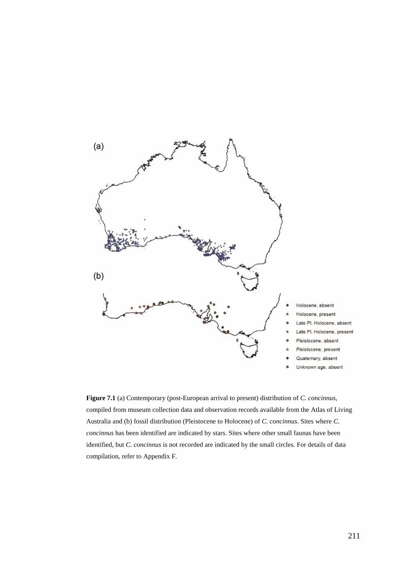
211
Figure 7.1 (a) Contemporary (post-European arrival to present) distribution of C. concinnus,
compiled from museum collection data and observation records available from the Atlas of Living
Australia and (b) fossil distribution (Pleistocene to Holocene) of C. concinnus. Sites where C.
concinnus has been identified are indicated by stars. Sites where other small faunas have been
identified, but C. concinnus is not recorded are indicated by the small circles. For details of data
compilation, refer to Appendix F.
212
The research presented in chapter five deliberately ignored temporal patterns within
the examined assemblages. While this may be considered a limitation of the work,
temporal patterns were thoroughly examined in chapter six. The primary aim of
chapter five was to provide an up-to-date list of the small mammal faunas of Late
Pleistocene–Holocene Naracoorte for the research community and to detail the
sampling protocols used to generate the faunal databases for the studied
assemblages. Given the significance of the fossil assemblages in providing pre-
European and Pleistocene distributions for extant and extinct faunas, it is imperative
that the underlying data (that is, taxonomic lists) are continually revised and
checked for accuracy.
Additionally, the fossil specimens for Wet Cave were formally assigned field
numbers only and the original database was no longer available (M. McDowell,
pers. comm.). All specimens identified in the current study were registered to either
the Flinders University Fossil Register or the SAM Palaeontology Collection, under
the direction of E. Reed. Electronic databases of the specimens and their
registrations have been produced as part of this thesis and have been integrated into
the collection management systems of the SAM (M. Binnie) and Flinders
University (E. Reed and A. Macken). These processes are critical for the
accountability of the research presented in the thesis and to facilitate access and
interpretation by others.
As c. 23,500 specimens were identified from the assemblages of Wet, Blanche and
Robertson Cave entrance chamber, there is no doubt that there are some errors in
the identification of some specimens examined for this thesis. However, all attempts
were made to ensure that identifications were accurate through the use of
comparative specimens from a wide range of collections (including both modern
and fossil), reference to descriptions in the literature and discussions with other
researchers experienced in small mammal identification. As some taxonomic groups
are more difficult to identify to species level than others, it is suggested that future
work target the following groups to more clearly define diagnostic characters and
intraspecific variation: Pseudomys auritus versus Pseudomys australis, and
Pseudomys novaehollandiae versus Pseudomys apodemoides. The two undiagnosed
213
Dasyuridae taxa (Dasyuridae sp. 1 and Sminthopsis sp. 1) also clearly require
further examination to assess if they are known or new taxa.
In chapter six, the sedimentary, stratigraphic, chronological and species diversity
data were integrated for the faunal analyses. Chapter six addressed the primary aims
of the thesis relating to the detection and assessment of natural variation in the small
mammal assemblages of Wet and Blanche caves, and the relationship between
variation and resilience.
The faunal analyses were structured around a comparison of site versus temporal
variation of different palaeocommunity metrics through time. This approach
enabled an assessment of the statistical significance of temporal variation across all
metrics. The use of an a priori defined ecological hierarchy combining the metric
scale of Rahel (1990) and terminology of Bennington and Bambach (1996)
provided a novel basis for assessing the ecological significance of observed
variability.
There were a number of key findings from the faunal analyses, summarised below:
1. The small mammal palaeocommunity was stable through the early
glacial period and LGM, c. 51.4 to 17.1 kyr BP. This stability was
observed despite changes in palaeoclimatic and environmental conditions at
different temporal scales and suggests that such changes were within limits
that could be tolerated by the palaeocommunity either through adaptation,
resilience and/or intrinsic population processes. The resilience of the
palaeocommunity to the LGM contrasts with a general assumption that this
period was associated with local declines in biodiversity in Australia
(McDowell et al., 2013). The lack of significant palaeocommunity change at
the LGM observed in the Wet and Blanche caves faunas may reflect the
influence of either local refugial dynamics or that a resilient faunal
community was already established by the start of the early glacial period.
Alternatively, climatic and environmental conditions at the LGM may not
have differed greatly from those of the preceding 10,000 years, for which
214
there is evidence of fluctuating but sustained cool mean temperatures (Lopes
dos Santos et al., 2012).
2. At least one significant palaeocommunity reorganisation was detected
over the post-LGM deglaciation. This palaeocommunity reorganisation
was evidenced by a statistically significant decline in species richness from
c. 17.1 to 16.7 kyr BP and was correlated with SSTs warming beyond 16°C.
A second possible change in palaeocommunity type was indicated by a
decline in rank-order abundance of the palaeocommunity from c. 10.8 to
10.5 kyr BP and was associated with a continued warming of mean SSTs
past 18°C. These observations reflect palaeoclimatic thresholds of
successive palaeocommunity types for small mammals of south-eastern
South Australia. The first palaeocommunity reorganisation lagged behind
the onset of post-glacial warming, suggesting that temperature thresholds
may be more important in structuring faunal communities than shifts
towards warming or cooling per se.
3. For some variables, site-based sampling variation was similar to, or
greater than, temporal variation. This limited the significance that could
be drawn from observed changes through the depositional sequences and
was particularly the case for individual species proportions. For the majority
of species, random sampling effects obscured temporal effects, cautioning
against the use of species proportions to assess species responses to past
palaeoclimatic and environmental changes. It also cautions against the use
of species abundances as a basis for palaeoenvironmental reconstructions.
However, in some cases, individual species relative abundances were
adequately sampled. The similarity observed between the relative abundance
trends of species between Wet and Blanche caves also suggests that in some
cases, changes in relative abundances are accurately represented in fossil
assemblages. These findings advocate the use of a range of statistical tests to
discern those trends that may be considered ecologically significant and
those that represent ‘noise’. If palaeoecological trends are to be used to
inform biodiversity conservation strategies, it is imperative that the observed
data are robust and critically evaluated.
215
4. Mesoscale analyses revealed significant change that was obscured or
‘time-averaged’ at the macroscale. While the macroscale analyses
revealed palaeocommunity reorganisation between units C and E in Wet
Cave, the mesoscale analyses showed that significant palaeocommunity
changes occurred at discrete times over the deglacial period. The two
timescales available in the deposits provided the first opportunity to
compare longer term trends (e.g., early glacial versus LGM versus
deglaciation) against shorter-term climate and environmental fluctuations
both for the Naracoorte Caves and other vertebrate fossil sites in Australia.
Each of these findings leads to new research questions that may be explored in
future analysis of the Wet and Blanche caves faunas, and those of other deposits of
the Naracoorte Caves. Of interest is the relationship between palaeocommunity
restructuring and local vegetation dynamics. The published pollen record for
Blanche Cave provides only a coarse reference to local vegetation; however, a more
detailed and finely resolved pollen record is available and is in preparation by E.
Reed (pers. comm.). Cross-correlation of the palaeocommunity types with the
detailed pollen record will enable a test for environmental thresholds in terms of a
range of new variables including dominant canopy species (e.g., Eucalyptus versus
Banksia) dominant understorey composition (e.g., shrubby heath versus grassland)
and relative vegetation density (e.g., open versus closed woodland) at a finer
palynological and temporal scale.
Despite the caution applied to interpretation of the relative abundances of individual
species in the thesis, a suite of new questions may be examined for those taxa where
the data are more reliable. Of particular interest is the relative role of intrinsic (such
as metapopulation dynamics, local adaptation) versus extrinsic processes (e.g.,
habitat heterogeneity) to the long-term persistence of individual species through the
Quaternary in south-eastern South Australia. As noted in the thesis, the faunas
preserved in the Naracoorte Caves are commonly used to argue for the preservation
of a mosaic of vegetation types proximal to the caves through the Quaternary. This
observation is significant to discussions of biogeographic refugia in southern
Australia, which are considered to be places that have maintained a range of habitat
types through periods of climate stress (Byrne, 2008). The diverse and complex
216
topography of south-eastern South Australia is expected to have played an
important role in maintaining habitat heterogeneity and hence, the long-term
persistence of individual taxa. However, no specific tests of this hypothesis have
been made nor have other factors such as evolutionary adaptation (e.g., change in
body size or dietary breadth) been examined.
Future research will test the relative role of extrinsic and intrinsic processes in the
long-term persistence of individual small mammal species through the Late
Quaternary. This will also involve identifying potential environmental and intrinsic
correlates of the observed increases in abundance of Sminthopsis murina,
Pseudomys apodemoides and Cercartetus nanus over the deglacial period. Each of
these taxa maintained a presence within the region during MIS-3 and the LGM, but
at low relative abundance when compared with other species and their later
expansions (Fig. 6.11). The drivers of concurrent declines in relative abundance of
Perameles bougainville and Pseudomys australis are also of interest.
The relative abundance data for these species and others adequately sampled in Wet
and Blanche Caves could also be used to examine habitat-faunal associations of the
past. Cross-correlation of individual species with the high-resolution pollen record
will enable a test of the stability of plant-faunal associations through time and a
comparison against species contemporary habitat preferences to examine how much
niche contraction or change has occurred as a result of European landscape
disturbance. A fire history for the Late Quaternary from charcoal sequences in the
deposits could also be used as a basis for identifying temporal patterns in species-
fire interactions.
Another area of future research for the Naracoorte Caves is to define the
composition and structure of the Holocene palaeocommunity and determine how
local faunas responded to increased regional seasonality and continuing warming
through this period (Kemp et al., 2012; Lopes dos Santos et al., 2012). Of particular
interest is to identify the timing and environmental correlates of local extinction of
small mammal species that persisted through Pleistocene climate changes but which
are now absent from south-eastern South Australia (e.g., Pseudomys auritus and
Pseudomys australis).
217
Future research directions will also involve more comparative faunal analyses to
assess longer-term patterns of palaeocommunity variability and the structure of
successive faunal communities through the Pleistocene by comparing the faunas of
Wet and Blanche caves with those of Cathedral Cave and Grant Hall. Spatial-
temporal patterns of palaeocommunity structure could also be examined through a
comparison of the Wet and Blanche Cave faunas with those from the two deposits
in Robertson Cave. The excavation of other Late Quaternary aged fossil sites within
the Naracoorte Caves by E. Reed (pers. comm.) presents further opportunities to
explore palaeocommunity variability and responses to climatic and environmental
change at different time scales, likely to enhance our understanding of the patterns
and drivers observed in the current thesis.
An important future research direction is to link palaeocommunity patterns
observed in the Naracoorte Caves to other localities to assess spatial-temporal
patterns of species occurrence and palaeocommunity structure. Target locations
include south-western Victoria and the Lower South East of South Australia, and
the Murray Mallee region, forming a latitudinal gradient south and north of the
Naracoorte Caves, respectively. The aim of this research will be to determine
patterns of latitudinal range contraction and expansion of individual taxa to better
understand the spatial dynamics associated with the responses of individual species
and palaeocommunity types to climate change.
Final Synthesis The theoretical relationship between natural variation and resilience provided a
framework for the research presented in this thesis. These concepts are increasing
being applied to biodiversity conservation strategies, but rarely are baseline data on
the constraints, processes and patterns of changes in diversity in response to
disturbances across different temporal, spatial and ecological scales available.
Palaeoecological assemblages are increasingly recognised as a source of
information on the types of changes and responses that occur across scales within
ecological communities through time. However, rarely are theoretical and statistical
frameworks used in the assessment of temporal patterns of change in
palaeoecology, despite the arguments forwarded by Erwin (2009) and Rull (2012).
218
In the analysis of the Late Quaternary fossil assemblages of Wet and Blanche caves
presented here, concepts relating to natural variation and resilience provided a way
of linking observations in the fossil record to current and future biodiversity
conservation strategies. This was achieved primarily by addressing key knowledge
gaps about the normal types of response to different patterns of environmental and
climatic change, and the time scales over which they are expressed. Of particular
focus for this thesis were the responses of the small mammal palaeocommunity to
both short and long-term patterns of climate change, the natural range of variation
exhibited by the small mammal palaeocommunity at different ecological and
temporal scales and the limits of resilience, or thresholds beyond which the
palaeocommunity shifted to a new state.
The main finding of the thesis in relation to these questions is that patterns of
variation observed in fossil records are highly dependent upon the scales at which
they are measured. This was not unexpected in light of the discussions presented in
the literature review. However, the research presented here provides the first
quantification of these differences in the study of vertebrate fossil assemblages of
the Naracoorte Caves and Australia more broadly.
The assemblages of Wet and Blanche caves show that palaeocommunity types
(defined by a given rank-order abundance structure) can be persistent for thousands
of years during periods of highly variable climatic conditions, even at different
scales of time-averaging. The persistent palaeocommunity type of the early glacial
and LGM periods reflects the resilience of the palaeocommunity in terms of
structure, richness and composition to frequent temperature fluctuations within the
range of c. 10 to 16°C (SSTs; Lopes dos Santos et al., 2012) combined with broad
scale restructuring of vegetation communities. This suggests that it is not
disturbance per se that leads to shifts between community/ecosystem states, but
disturbance beyond thresholds within which particular states can persist. A similar
conclusion was drawn by Rodriguez (2004) based on observed ecological stability
of mammal communities in the Mediterranean during the Early to Middle
Pleistocene. A key priority of research on contemporary ecosystems should then be
to model and predict thresholds within which community structures can be
maintained.
219
At the finer temporal scale available in the deposits, the small mammal assemblages
showed that state shifts may or may not be preceded by gradual palaeocommunity
changes. For example, beta diversity measures at the mesoscale indicated a gradual
decline in similarity between the successive palaeocommunity samples through
phases E1 to E5, culminating in a shift to a new palaeocommunity type at phase E6.
This is not surprising given the nature of the climate thresholds detected for the
palaeocommunities. In both cases of palaeocommunity change, the thresholds were
associated with continued warming, rather than short-term fluctuations in
temperatures as was observed over the early glacial period and LGM. However, in
comparison to the second palaeocommunity reorganisation, the first significant
change in palaeocommunity type was not the result of a gradual trend. It instead
occurred as an abrupt decline in species richness, without prior indication of
changes operating within the palaeocommunity. These contrasting patterns reflect
the influence of both intrinsic and extrinsic responses of the small mammal faunas
to climate change.
Intrinsic responses are associated with non-linear ecological processes, thresholds
and tipping points (Williams et al., 2011). Such responses are characterised by
variable timings and rates of change among species and localities in response to
progressive climate change. Intrinsic responses are expected to best explain the
palaeocommunity shift observed between phases E5 and E6 at the end of the
Pleistocene. Evidence for non-synchronous rates and timing of changes among
species through the deglaciation is reflected in Fig 6.11. For example, both
Pseudomys apodemoides and Cercartetus nanus increased in relative abundance
over the deglacial period. However, the increase in relative abundance in P.
apodemoides began from phase C2. By comparison, the abundance of C. nanus
remained at very low levels until it rapidly increased between phase E5 and E6.
While asynchronous fluctuations in species relative abundances are evident through
the early glacial period and LGM, they were insufficient to lead to a new rank-order
abundance structure within the palaeocommunity as a whole.
In contrast to intrinsic responses, extrinsic ecological changes are driven by
external, abrupt climate changes and are characterised by synchronous responses of
species within and between localities (Williams et al., 2011). While not all species
220
demonstrated a significant change in relative abundance between phases C2 and E1,
the significant decline in species richness observed shows that the ranges of a
number of species contracted away from the Naracoorte Caves region at the same
time.
These contrasting intrinsic and extrinsic responses to climate change show that
there may or may not be early warnings for community level shifts. In comparison
to Hadly and Barnosky (2009) who argued that changes in species abundance signal
environmental and climatic impacts on communities, species relative abundances in
the assemblages of Wet and Blanche caves were not always associated with the
palaeoclimatic and environmental variables. They were also not always statistically
significant or ecologically significant in terms of impacts at higher levels of
community-structure. This suggests that changes in the relative abundances of
individual species may not best reflect the nature of palaeoenvironmental changes
of the past or be a reliable indicator for future climate change or other
environmental effects. Instead, measures that take account of species abundances
within a community as a whole may be more reliable indicators of community
changes.
However, where the relative abundances of individual species were more reliably
sampled, they provide evidence for individualistic species responses to past
disturbances. These asynchronous changes in species abundances observed in the
Wet and Blanche cave assemblages suggest that future climate change will impact
on species within communities in different ways, even if they are considered to
have similar ecological niches and tolerance ranges. A similar finding has been
found in studies from other continents (e.g., Stewart, 2008; Stewart et al., 2009).
From a biodiversity conservation perspective, this suggests that species responses to
disturbances may be unpredictable, arguing for regional evaluation of population
distributions, size and connectivity. Maintaining the capacity of individuals to
disperse to new habitats and/or sustain populations across a range of localities is
expected to be critical strategies for building not only the resilience of individual
species, but communities. The latter emerges as a result of the asynchrony of
changes in individual species. Clearly then, synchronous changes in the relative
221
abundances of individual species may be used to identify communities at risk of
structural change.
These observations advocate for biodiversity conservation approaches that monitor
the abundances of individual species across their range and the structure of local
communities. In combining these two strategies, multiple ecological and spatial
scales are considered. At the present time, many longer-term programs monitor
species presence/absence only. This is because it is time consuming and more
difficult to measure species abundances. However, the fossil assemblages of Wet
and Blanche caves show that the composition of a community may be stable for
very long periods of time, even with the sporadic occurrence of vagrants (e.g.,
Dasycercus sp.) or rare taxa. Further, some species may persist at very low
abundance over multiple sampling periods (e.g., Cercartetus nanus) before
dramatically increasing or decreasing in abundance. Presence/absence data cannot
provide insight into these types of changes.
In contrast to the approach adopted in this thesis, other palaeoecological studies
have focussed on the ecological traits and functions represented in a fossil
assemblage to define palaeocommunity types and hence, examine variability
through time (e.g., Rodriguez, 2004). These approaches stem from a prevailing
trend that, regardless of the species that fill ecological niches within a given
ecosystem through time, ecosystems generally demonstrate long term structural and
functional persistence (Rodriguez, 2004; Hadly and Barnosky, 2009). As such,
ecosystems may be best defined by their ecological traits, rather than on a
taxonomic basis.
Palaeocommunities were defined in this thesis based on taxonomic rather than
ecological traits because taxonomic based diversity and composition of the study
assemblages were poorly understood. Further, any approach that used ecological
traits would be severely limited by the bias in the fossil assemblages towards small
mammals. As a consequence of this bias, the diversity and richness of functional
groups is restricted by the poor representation of large mammals (body mass .2.5
kg) in the assemblages and the exclusion of non-mammalian faunas from this study.
Nonetheless, there is an important question that arises from these contrasting
222
approaches and that is, how do we recognise or define ‘normal’ or ‘problematic’
patterns of variation in species composition and richness if the trophic and size
structure of the community remains constant through time, and visa-versa?
Ultimately, the answer to this question is best informed by the values of society
regarding goals. In particular, the relative importance of preserving ecosystem
functions versus communities and species. For example, Walker (1992) argues that
it is more effective to manage for ecosystem function than individual species. In
contrast, the Australian Draft Biodiversity Conservation Strategy identifies the
retention of biodiversity values and critical ecosystem functions as the first of six
priorities to build ecological resilience. This presents a challenging conflict between
the conservation of individual species and maintaining ecosystem structure and
function. Palaeoecological information about the relationship between taxonomic
and ecological variability and resilience are imperative to addressing this conflict.
Finally, it is important to acknowledge that the temporal scales of the fossil
assemblages clearly exceed the time-scales over which ecosystems can be
monitored by researchers today and the rate at which anthropogenic climate change
is expected to impact on local communities. However, the macro- and mesoscale
trends documented in Wet and Blanche caves provide a backdrop against which
decadal trends may be compared. Seasonal fluctuations in species abundances and
the boom-bust cycles common in many Australian small mammals reflect natural
variation within yearly and decadal time periods. Research programs that can nest
these shorter term patterns within broader temporal scales will be critical for
identifying and mediating climate-change impacts into the future.
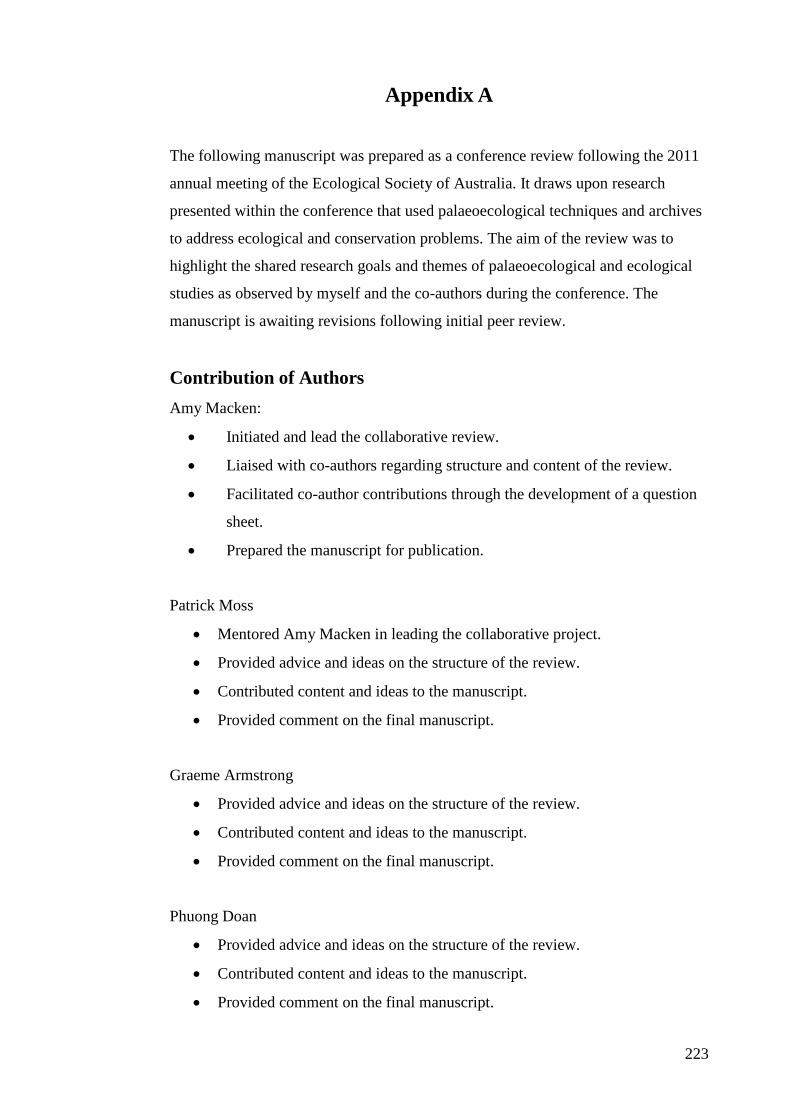
223
Appendix A
The following manuscript was prepared as a conference review following the 2011
annual meeting of the Ecological Society of Australia. It draws upon research
presented within the conference that used palaeoecological techniques and archives
to address ecological and conservation problems. The aim of the review was to
highlight the shared research goals and themes of palaeoecological and ecological
studies as observed by myself and the co-authors during the conference. The
manuscript is awaiting revisions following initial peer review.
Contribution of Authors Amy Macken:
• Initiated and lead the collaborative review.
• Liaised with co-authors regarding structure and content of the review.
• Facilitated co-author contributions through the development of a question
sheet.
• Prepared the manuscript for publication.
Patrick Moss
• Mentored Amy Macken in leading the collaborative project.
• Provided advice and ideas on the structure of the review.
• Contributed content and ideas to the manuscript.
• Provided comment on the final manuscript.
Graeme Armstrong
• Provided advice and ideas on the structure of the review.
• Contributed content and ideas to the manuscript.
• Provided comment on the final manuscript.
Phuong Doan
• Provided advice and ideas on the structure of the review.
• Contributed content and ideas to the manuscript.
• Provided comment on the final manuscript.

224
Beth Gott
• Provided advice and ideas on the structure of the review.
• Contributed content and ideas to the manuscript.
• Provided comment on the final manuscript.
Rosie Grundell
• Provided advice and ideas on the structure of the review.
• Contributed content and ideas to the manuscript.
• Provided comment on the final manuscript.
Chris Johnson
• Provided advice and ideas on the structure of the review.
• Contributed content and ideas to the manuscript.
• Provided comment on the final manuscript.
Matthew McDowell:
• Provided advice and ideas on the structure of the review.
• Contributed content and ideas to the manuscript.
• Provided comment on the final manuscript.
Jamie Wood
• Provided advice and ideas on the structure of the review.
• Contributed content and ideas to the manuscript.
• Provided comment on the final manuscript.
Craig Woodward
• Provided advice and ideas on the structure of the review.
• Contributed content and ideas to the manuscript.
• Provided comment on the final manuscript.

225
Signed .................................................................................. Date ............................
Amy Macken
School of Biological Sciences, Flinders University
Signed .................................................................................. Date ............................
Patrick Moss
School of Geography, Planning and Environmental Management, The University of
Queensland
Signed .................................................................................. Date ............................
Graeme Armstrong
Griffith School of Environment
Signed ................................................................................. Date ............................
Phuong Doan
School of Science, Information Technology and Engineering, University of Ballarat
Signed .................................................................................. Date ............................
Beth Gott
School of Biological Sciences, Monash University
Signed .................................................................................. Date
Rosie Grundell
School of Science, Information Technology and Engineering, University of Ballarat
Signed .................................................................................. Date ............................
Chris Johnson
School of Zoology, University of Tasmania
Signed .................................................................................. Date ............................
Matthew McDowell
School of Biological Science, Flinders University

226
Signed ................................................................................. Date ............................
Jamie Wood
Landcare Research
Signed .................................................................................. Date ............................
Craig Woodward
School of Geography, Planning and Environmental Management, The University of
Queensland
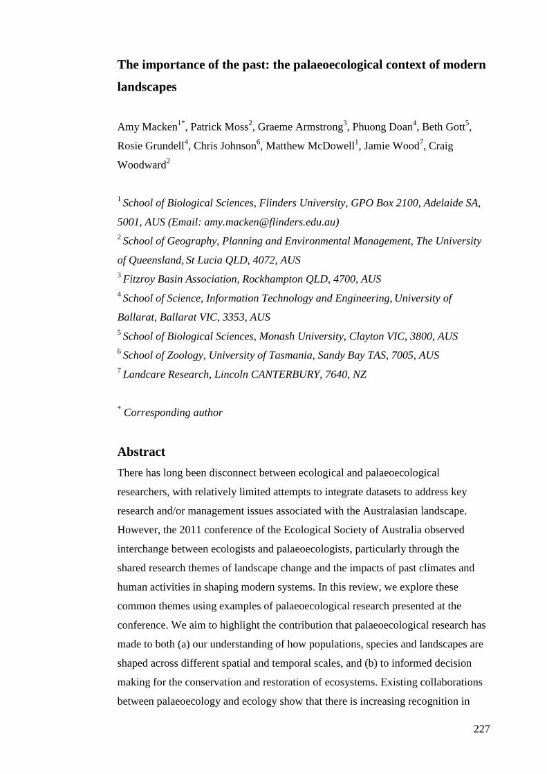
227
The importance of the past: the palaeoecological context of modern
landscapes
Amy Macken1*, Patrick Moss2, Graeme Armstrong3, Phuong Doan4, Beth Gott5,
Rosie Grundell4, Chris Johnson6, Matthew McDowell1, Jamie Wood7, Craig
Woodward2
1 School of Biological Sciences, Flinders University, GPO Box 2100, Adelaide SA,
5001, AUS (Email: [email protected]) 2 School of Geography, Planning and Environmental Management, The University
of Queensland, St Lucia QLD, 4072, AUS 3 Fitzroy Basin Association, Rockhampton QLD, 4700, AUS 4 School of Science, Information Technology and Engineering, University of
Ballarat, Ballarat VIC, 3353, AUS 5 School of Biological Sciences, Monash University, Clayton VIC, 3800, AUS 6 School of Zoology, University of Tasmania, Sandy Bay TAS, 7005, AUS 7 Landcare Research, Lincoln CANTERBURY, 7640, NZ
* Corresponding author
Abstract There has long been disconnect between ecological and palaeoecological
researchers, with relatively limited attempts to integrate datasets to address key
research and/or management issues associated with the Australasian landscape.
However, the 2011 conference of the Ecological Society of Australia observed
interchange between ecologists and palaeoecologists, particularly through the
shared research themes of landscape change and the impacts of past climates and
human activities in shaping modern systems. In this review, we explore these
common themes using examples of palaeoecological research presented at the
conference. We aim to highlight the contribution that palaeoecological research has
made to both (a) our understanding of how populations, species and landscapes are
shaped across different spatial and temporal scales, and (b) to informed decision
making for the conservation and restoration of ecosystems. Existing collaborations
between palaeoecology and ecology show that there is increasing recognition in
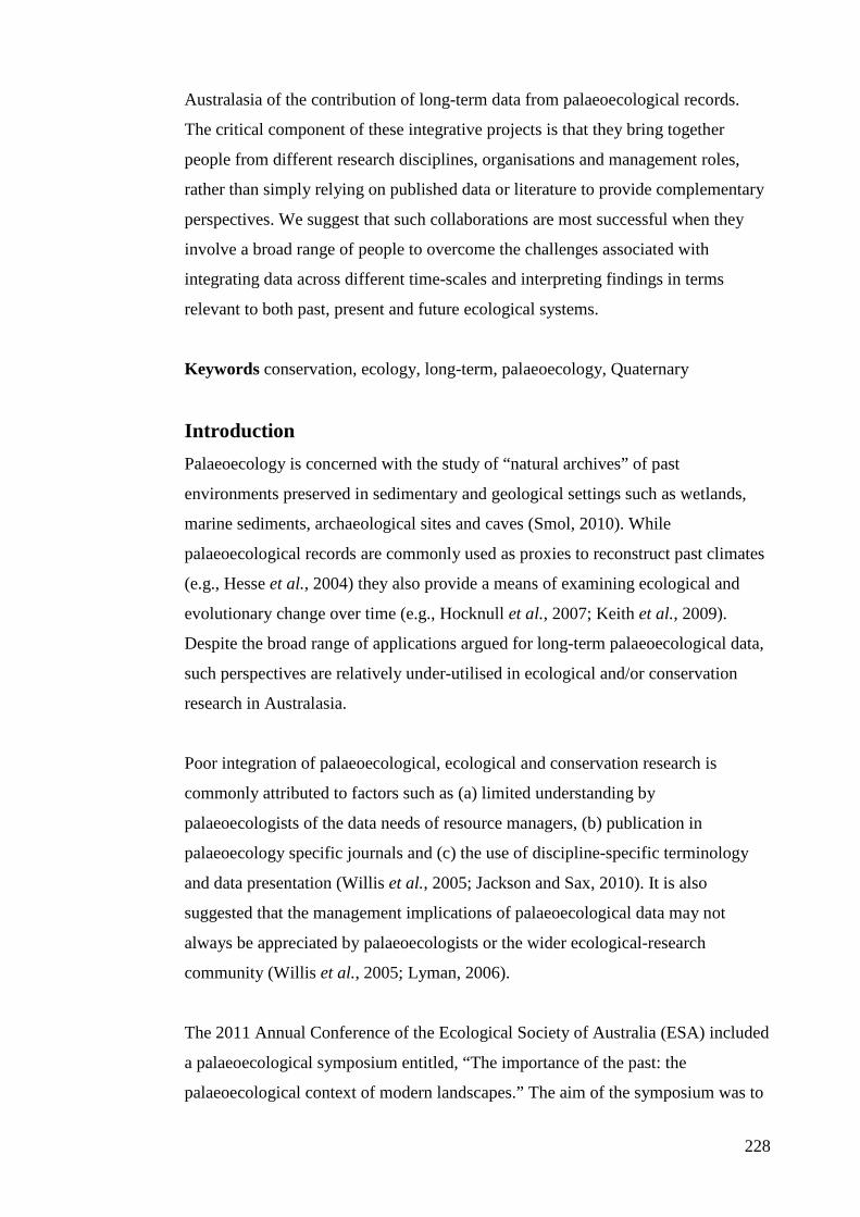
228
Australasia of the contribution of long-term data from palaeoecological records.
The critical component of these integrative projects is that they bring together
people from different research disciplines, organisations and management roles,
rather than simply relying on published data or literature to provide complementary
perspectives. We suggest that such collaborations are most successful when they
involve a broad range of people to overcome the challenges associated with
integrating data across different time-scales and interpreting findings in terms
relevant to both past, present and future ecological systems.
Keywords conservation, ecology, long-term, palaeoecology, Quaternary
Introduction Palaeoecology is concerned with the study of “natural archives” of past
environments preserved in sedimentary and geological settings such as wetlands,
marine sediments, archaeological sites and caves (Smol, 2010). While
palaeoecological records are commonly used as proxies to reconstruct past climates
(e.g., Hesse et al., 2004) they also provide a means of examining ecological and
evolutionary change over time (e.g., Hocknull et al., 2007; Keith et al., 2009).
Despite the broad range of applications argued for long-term palaeoecological data,
such perspectives are relatively under-utilised in ecological and/or conservation
research in Australasia.
Poor integration of palaeoecological, ecological and conservation research is
commonly attributed to factors such as (a) limited understanding by
palaeoecologists of the data needs of resource managers, (b) publication in
palaeoecology specific journals and (c) the use of discipline-specific terminology
and data presentation (Willis et al., 2005; Jackson and Sax, 2010). It is also
suggested that the management implications of palaeoecological data may not
always be appreciated by palaeoecologists or the wider ecological-research
community (Willis et al., 2005; Lyman, 2006).
The 2011 Annual Conference of the Ecological Society of Australia (ESA) included
a palaeoecological symposium entitled, “The importance of the past: the
palaeoecological context of modern landscapes.” The aim of the symposium was to
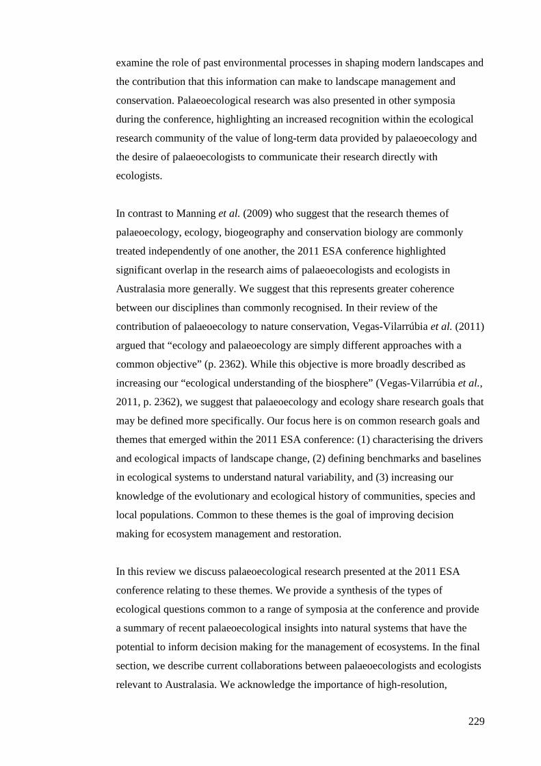
229
examine the role of past environmental processes in shaping modern landscapes and
the contribution that this information can make to landscape management and
conservation. Palaeoecological research was also presented in other symposia
during the conference, highlighting an increased recognition within the ecological
research community of the value of long-term data provided by palaeoecology and
the desire of palaeoecologists to communicate their research directly with
ecologists.
In contrast to Manning et al. (2009) who suggest that the research themes of
palaeoecology, ecology, biogeography and conservation biology are commonly
treated independently of one another, the 2011 ESA conference highlighted
significant overlap in the research aims of palaeoecologists and ecologists in
Australasia more generally. We suggest that this represents greater coherence
between our disciplines than commonly recognised. In their review of the
contribution of palaeoecology to nature conservation, Vegas-Vilarrúbia et al. (2011)
argued that “ecology and palaeoecology are simply different approaches with a
common objective” (p. 2362). While this objective is more broadly described as
increasing our “ecological understanding of the biosphere” (Vegas-Vilarrúbia et al.,
2011, p. 2362), we suggest that palaeoecology and ecology share research goals that
may be defined more specifically. Our focus here is on common research goals and
themes that emerged within the 2011 ESA conference: (1) characterising the drivers
and ecological impacts of landscape change, (2) defining benchmarks and baselines
in ecological systems to understand natural variability, and (3) increasing our
knowledge of the evolutionary and ecological history of communities, species and
local populations. Common to these themes is the goal of improving decision
making for ecosystem management and restoration.
In this review we discuss palaeoecological research presented at the 2011 ESA
conference relating to these themes. We provide a synthesis of the types of
ecological questions common to a range of symposia at the conference and provide
a summary of recent palaeoecological insights into natural systems that have the
potential to inform decision making for the management of ecosystems. In the final
section, we describe current collaborations between palaeoecologists and ecologists
relevant to Australasia. We acknowledge the importance of high-resolution,
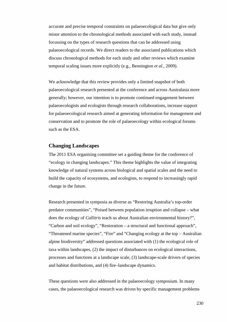
230
accurate and precise temporal constraints on palaeoecological data but give only
minor attention to the chronological methods associated with each study, instead
focussing on the types of research questions that can be addressed using
palaeoecological records. We direct readers to the associated publications which
discuss chronological methods for each study and other reviews which examine
temporal scaling issues more explicitly (e.g., Bennington et al., 2009).
We acknowledge that this review provides only a limited snapshot of both
palaeoecological research presented at the conference and across Australasia more
generally; however, our intention is to promote continued engagement between
palaeoecologists and ecologists through research collaborations, increase support
for palaeoecological research aimed at generating information for management and
conservation and to promote the role of palaeoecology within ecological forums
such as the ESA.
Changing Landscapes The 2011 ESA organising committee set a guiding theme for the conference of
“ecology in changing landscapes.” This theme highlights the value of integrating
knowledge of natural systems across biological and spatial scales and the need to
build the capacity of ecosystems, and ecologists, to respond to increasingly rapid
change in the future.
Research presented in symposia as diverse as “Restoring Australia’s top-order
predator communities”, “Poised between population irruption and collapse – what
does the ecology of Callitris teach us about Australian environmental history?”,
“Carbon and soil ecology”, “Restoration – a structural and functional approach”,
“Threatened marine species”, “Fire” and “Changing ecology at the top – Australian
alpine biodiversity” addressed questions associated with (1) the ecological role of
taxa within landscapes, (2) the impact of disturbances on ecological interactions,
processes and functions at a landscape scale, (3) landscape-scale drivers of species
and habitat distributions, and (4) fire–landscape dynamics.
These questions were also addressed in the palaeoecology symposium. In many
cases, the palaeoecological research was driven by specific management problems
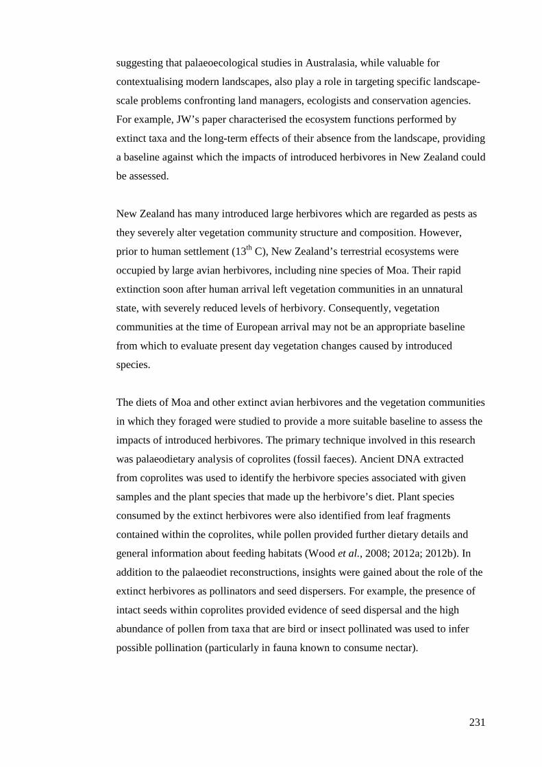
231
suggesting that palaeoecological studies in Australasia, while valuable for
contextualising modern landscapes, also play a role in targeting specific landscape-
scale problems confronting land managers, ecologists and conservation agencies.
For example, JW’s paper characterised the ecosystem functions performed by
extinct taxa and the long-term effects of their absence from the landscape, providing
a baseline against which the impacts of introduced herbivores in New Zealand could
be assessed.
New Zealand has many introduced large herbivores which are regarded as pests as
they severely alter vegetation community structure and composition. However,
prior to human settlement (13th C), New Zealand’s terrestrial ecosystems were
occupied by large avian herbivores, including nine species of Moa. Their rapid
extinction soon after human arrival left vegetation communities in an unnatural
state, with severely reduced levels of herbivory. Consequently, vegetation
communities at the time of European arrival may not be an appropriate baseline
from which to evaluate present day vegetation changes caused by introduced
species.
The diets of Moa and other extinct avian herbivores and the vegetation communities
in which they foraged were studied to provide a more suitable baseline to assess the
impacts of introduced herbivores. The primary technique involved in this research
was palaeodietary analysis of coprolites (fossil faeces). Ancient DNA extracted
from coprolites was used to identify the herbivore species associated with given
samples and the plant species that made up the herbivore’s diet. Plant species
consumed by the extinct herbivores were also identified from leaf fragments
contained within the coprolites, while pollen provided further dietary details and
general information about feeding habitats (Wood et al., 2008; 2012a; 2012b). In
addition to the palaeodiet reconstructions, insights were gained about the role of the
extinct herbivores as pollinators and seed dispersers. For example, the presence of
intact seeds within coprolites provided evidence of seed dispersal and the high
abundance of pollen from taxa that are bird or insect pollinated was used to infer
possible pollination (particularly in fauna known to consume nectar).
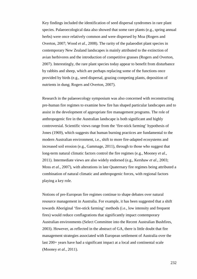
232
Key findings included the identification of seed dispersal syndromes in rare plant
species. Palaeoecological data also showed that some rare plants (e.g., spring annual
herbs) were once relatively common and were dispersed by Moa (Rogers and
Overton, 2007; Wood et al., 2008). The rarity of the palaeodiet plant species in
contemporary New Zealand landscapes is mainly attributed to the extinction of
avian herbivores and the introduction of competitive grasses (Rogers and Overton,
2007). Interestingly, the rare plant species today appear to benefit from disturbance
by rabbits and sheep, which are perhaps replacing some of the functions once
provided by birds (e.g., seed dispersal, grazing competing plants, deposition of
nutrients in dung; Rogers and Overton, 2007).
Research in the palaeoecology symposium was also concerned with reconstructing
pre-human fire regimes to examine how fire has shaped particular landscapes and to
assist in the development of appropriate fire management programs. The role of
anthropogenic fire in the Australian landscape is both significant and highly
controversial. Scientific views range from the ‘fire-stick farming’ hypothesis of
Jones (1969), which suggests that human burning practices are fundamental to the
modern Australian environment, i.e., shift to more fire-adapted ecosystems and
increased soil erosion (e.g., Gammage, 2011), through to those who suggest that
long-term natural climatic factors control the fire regimes (e.g., Mooney et al.,
2011). Intermediate views are also widely endorsed (e.g., Kershaw et al., 2003;
Moss et al., 2007), with alterations in late Quaternary fire regimes being attributed a
combination of natural climatic and anthropogenic forces, with regional factors
playing a key role.
Notions of pre-European fire regimes continue to shape debates over natural
resource management in Australia. For example, it has been suggested that a shift
towards Aboriginal ‘fire-stick farming’ methods (i.e., low intensity and frequent
fires) would reduce conflagrations that significantly impact contemporary
Australian environments (Select Committee into the Recent Australian Bushfires,
2003). However, as reflected in the abstract of GA, there is little doubt that fire
management strategies associated with European settlement of Australia over the
last 200+ years have had a significant impact at a local and continental scale
(Mooney et al., 2011).
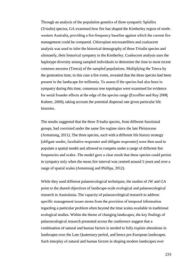
233
Through an analysis of the population genetics of three sympatric Spinifex
(Triodia) species, GA examined how fire has shaped the Kimberley region of north-
western Australia, providing a fire-frequency baseline against which the current fire
management could be compared. Chloroplast microsatellites and coalescent
analysis was used to infer the historical demography of three Triodia species and
ultimately, their historical sympatry in the Kimberley. Coalescent analysis uses the
haplotype diversity among sampled individuals to determine the time to most recent
common ancestor (Tmrca) of the sampled populations. Multiplying the Tmrca by
the generation time, in this case a fire event, revealed that the three species had been
present in the landscape for millennia. To assess if the species had also been in
sympatry during this time, consensus tree topologies were examined for evidence
for serial founder effects at the edge of the species range (Excoffier and Ray 2008;
Kuhner, 2009), taking account the potential dispersal rate given particular life
histories.
The results suggested that the three Triodia species, from different functional
groups, had coexisted under the same fire regime since the late Pleistocene
(Armstrong, 2011). The three species, each with a different life history strategy
(obligate seeder, facultative resprouter and obligate resprouter) were then used to
populate a spatial model and allowed to compete under a range of different fire
frequencies and scales. The model gave a clear result that these species could persist
in sympatry only when the mean fire interval was centred around 5 years and over a
range of spatial scales (Armstrong and Phillips, 2012).
While they used different palaeoecological techniques, the studies of JW and GA
point to the shared objectives of landscape-scale ecological and palaeoecological
research in Australasia. The capacity of palaeoecological research to address
specific management issues stems from the provision of temporal information
regarding a particular problem often beyond the time scales available in traditional
ecological studies. Within the theme of changing landscapes, the key findings of
palaeoecological research presented across the conference suggest that a
combination of natural and human factors is needed to fully explain alterations in
landscapes over the Late Quaternary period, and hence pre-European landscapes.
Such interplay of natural and human factors in shaping modern landscapes over
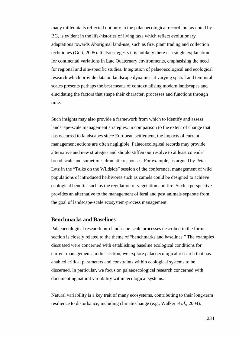
234
many millennia is reflected not only in the palaeoecological record, but as noted by
BG, is evident in the life-histories of living taxa which reflect evolutionary
adaptations towards Aboriginal land-use, such as fire, plant trading and collection
techniques (Gott, 2005). It also suggests it is unlikely there is a single explanation
for continental variations in Late Quaternary environments, emphasising the need
for regional and site-specific studies. Integration of palaeoecological and ecological
research which provide data on landscape dynamics at varying spatial and temporal
scales presents perhaps the best means of contextualising modern landscapes and
elucidating the factors that shape their character, processes and functions through
time.
Such insights may also provide a framework from which to identify and assess
landscape-scale management strategies. In comparison to the extent of change that
has occurred to landscapes since European settlement, the impacts of current
management actions are often negligible. Palaeoecological records may provide
alternative and new strategies and should stiffen our resolve to at least consider
broad-scale and sometimes dramatic responses. For example, as argued by Peter
Latz in the “Talks on the Wildside” session of the conference, management of wild
populations of introduced herbivores such as camels could be designed to achieve
ecological benefits such as the regulation of vegetation and fire. Such a perspective
provides an alternative to the management of feral and pest animals separate from
the goal of landscape-scale ecosystem-process management.
Benchmarks and Baselines Palaeoecological research into landscape-scale processes described in the former
section is closely related to the theme of “benchmarks and baselines.” The examples
discussed were concerned with establishing baseline ecological conditions for
current management. In this section, we explore palaeoecological research that has
enabled critical parameters and constraints within ecological systems to be
discerned. In particular, we focus on palaeoecological research concerned with
documenting natural variability within ecological systems.
Natural variability is a key trait of many ecosystems, contributing to their long-term
resilience to disturbance, including climate change (e.g., Walker et al., 2004).
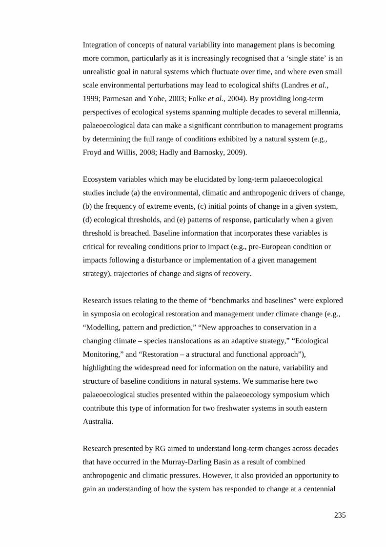
235
Integration of concepts of natural variability into management plans is becoming
more common, particularly as it is increasingly recognised that a ‘single state’ is an
unrealistic goal in natural systems which fluctuate over time, and where even small
scale environmental perturbations may lead to ecological shifts (Landres et al.,
1999; Parmesan and Yohe, 2003; Folke et al., 2004). By providing long-term
perspectives of ecological systems spanning multiple decades to several millennia,
palaeoecological data can make a significant contribution to management programs
by determining the full range of conditions exhibited by a natural system (e.g.,
Froyd and Willis, 2008; Hadly and Barnosky, 2009).
Ecosystem variables which may be elucidated by long-term palaeoecological
studies include (a) the environmental, climatic and anthropogenic drivers of change,
(b) the frequency of extreme events, (c) initial points of change in a given system,
(d) ecological thresholds, and (e) patterns of response, particularly when a given
threshold is breached. Baseline information that incorporates these variables is
critical for revealing conditions prior to impact (e.g., pre-European condition or
impacts following a disturbance or implementation of a given management
strategy), trajectories of change and signs of recovery.
Research issues relating to the theme of “benchmarks and baselines” were explored
in symposia on ecological restoration and management under climate change (e.g.,
“Modelling, pattern and prediction,” “New approaches to conservation in a
changing climate – species translocations as an adaptive strategy,” “Ecological
Monitoring,” and “Restoration – a structural and functional approach”),
highlighting the widespread need for information on the nature, variability and
structure of baseline conditions in natural systems. We summarise here two
palaeoecological studies presented within the palaeoecology symposium which
contribute this type of information for two freshwater systems in south eastern
Australia.
Research presented by RG aimed to understand long-term changes across decades
that have occurred in the Murray-Darling Basin as a result of combined
anthropogenic and climatic pressures. However, it also provided an opportunity to
gain an understanding of how the system has responded to change at a centennial
236
scale. Over the past 200 years since European settlement of Australia, the Murray-
Darling Basin has undergone significant changes in land use and water management
(Davis et al., 2001). There is little doubt the system is still responding to these
changes, in concert with a highly variable climate which makes the determination of
a baseline condition extremely difficult. Many wetlands are now so far removed
from their ‘natural condition’ that restoration attempts are largely futile (Gell,
2010).
While state switches in the wetlands of the river have been well documented (e.g.,
Ogden, 2000; Reid et al., 2007; Reid, 2008), little attention has been given to the
water-quality history of wetlands on the river and how the sediments from these
environments may be best studied to reveal pre- and post- European condition.
RG’s research was particularly concerned with the following questions: How has
water quality in the Sinclair Flat wetland of the lower River Murray changed
following European settlement and how does the present ecological condition of the
wetland compare to its historical range of variability?
The palaeoecological archives utilised in this research were diatoms sampled within
sedimentary cores from the study locality. Diatoms are unicellular micro algae
found in fresh water and marine systems. Many diatom species have narrow
tolerance limits which make them useful bioindictors and, as a result, they are
commonly used to monitor present day environmental conditions (e.g., Cook et al.,
2010; Ziemann and Schulz, 2011). Preservation of the silica cell walls of diatoms in
sedimentary sequences makes them useful palaeoecological proxies to reconstruct
the biological, physical and chemical variables of water bodies through time. By
providing information on a wide range of variables, diatoms are particularly
valuable as they enable the interaction of different abiotic and biotic factors to be
evaluated.
Historical changes to Sinclair Flat from the diatom record show a gradual transition
from a clear-water system favouring benthic species in the 1920s when river
regulation was introduced, to a plankton dominated system in the 1950s. By the
1960s, the Sinclair Flat was characterised by higher concentrations of epiphytic
diatoms suggesting increased macrophytic cover. Today, the wetland is a turbid,
237
nutrient enriched and mesosaline lagoon, attesting to the degraded state of the lower
River Murray (Grundell et al., 2012). Importantly, the long-term record from
Sinclair Flat revealed a gradual change in river conditions following river
regulation, rather than a single, short-term impact (Grundell et al., 2012).
Consequently, intermittent sampling is unlikely to have revealed the ecological
response of the system, enforcing the need for long-term studies of natural systems
for detecting trends and natural variability in complex ecological systems.
The second example is the current research of PD into the ecological function of
lakes of the Western Plains, Victoria through the last 5000 years. Many studies have
reconstructed Pleistocene climate variability in this region through the use of
bioindicators such as pollen, diatoms and ostracods (e.g., Gell et al., 1994; Jones et
al., 2001; Kershaw et al., 2004). These studies have revealed the close relationship
between changes in salinity and lake water levels to climate and climate variability
in this system; however, the impact of catchment and climatic changes on primary
productivity and producers remains largely unknown. The research of PD aims to
address this knowledge gap by examining primary productivity and phototrophic
community structure, measured from fossil pigments preserved in the lake
sediments.
At a local scale, drivers of change in primary producers in the lake systems are
expected to include local nutrient enrichment from diffuse and point sources of
sewage, agriculture and industrial wastes within the catchment. At a regional scale,
the pervasive nature of atmospheric nitrogen pollution is increasingly recognised as
a mechanism of change in lake systems while global climatic change is likely to
impact the nature and function of lakes via altered inputs of energy and other
materials.
Pigments produced by aquatic plants, algae and photosynthetic bacteria are useful
bioindicators as they represent the entire phototrophic community with a high
degree of taxon specificity (Wright and Jeffrey, 1997; Leavitt and Hodgson, 2001).
In PD’s current research, fossil pigments from the sediment cores will be detected
using High-performance Liquid Chromatography, an advanced technique that can
separate, qualify and quantify individual pigments in a sample (e.g., Chen et al.,
238
2001; Leavitt and Hodgson, 2001). Additional palaeoecological proxies (diatoms
and pollen) will also be correlated with the pigment data.
As these examples demonstrate, tracking environmental and ecological changes in
sediment records through time can reveal the impacts of human activity and natural
processes on ecological and environmental systems. They are also critical in
providing benchmarks and baselines against which managers can evaluate the
degree to which their restoration efforts are successful. Such baselines give insight
into the key constraints operating on natural systems at decadal to millennial time
scales, depending on the preservation and nature of the depositional environment.
In a recent review Batterbee et al. (2011) noted that palaeoecological records,
particularly those of freshwater systems, can provide an extension of long-term
monitoring data-sets. In some cases, palaeoecological records from sedimentary
deposits overlap in age with long-term monitoring programs, enabling cross-
validation between them (Batterbee et al., 2011). This is particularly relevant to the
palaeolimnological studies discussed here, where high resolution records of
seasonal to decadal conditions are commonly preserved in the finely laminated
sediments of freshwater systems. These records are particularly useful for the
investigation of human driven effects on natural systems that commonly operate
over short time frames.
Evolution and Ecology of Diversity As discussed for “benchmarks and baselines”, many research questions associated
with the theme of “evolution and ecology of diversity,” are common to the first
section which was concerned with “changing landscapes.” This overlap arises
because of the inherent links between ecosystem processes, landscape dynamics,
species geographic ranges and the distribution of diversity. In this section, we
examine the relationships between diversity at a given locality, the geographic
ranges of individual taxa and the evolutionary, ecological and historical factors that
shape them through time.
David Bowman’s opening plenary session set a vibrant tone for the conference,
encouraging continued curiosity of the natural world to drive ecological research.
239
He also challenged delegates to continue to develop and further their research into
the processes that structure ecosystems, rather than focussing solely on
documenting diversity. He argued that describing diversity is relatively easy in
comparison to the increasingly vital need to understand the interactions and
constraints which control diversity.
Palaeoecological research presented at the conference shows that palaeoecological
techniques have the potential to inform on ecological processes and, contrary to
general perceptions, commonly addresses complex ecological questions relating to
species interactions and their relationship with abiotic factors that shape the
distribution of diversity in the long-term. However, the examples also show that
information about past diversity is valuable as a baseline against which the extent
and rates of change in diversity of a given locality can be determined. Such
descriptions may be the only source of information from which we can identify at-
risk species and habitats and to provide a context when considering assertive
conservation actions such as translocations.
The presentation of MM in the palaeoecology symposium provides an example of
palaeoecological research concerned with reconstructing the past temporal and
spatial distribution of vertebrate faunas and the diversity of mammal communities
through time. Vertebrate fossil assemblages are preserved in a wide range of
environments and geological settings such as lake and riparian deposits, rock
shelters and caves, dune blowouts and human structures such as buildings and eaves
(e.g., Price and Sobbe, 2005; Hocknull et al., 2007; McDowell and Medlin, 2009).
The remains of vertebrates accumulate in these settings through natural attrition
such as pitfall entrapment into caves, death of inhabiting animals, mass-death
events, post-death transport of bone material and predatory accumulation by owls
and other raptors, humans or carnivorous mammals and reptiles (e.g., Reed and
Bourne, 2000; McDowell and Medlin, 2009).
MM highlighted the specific utility of late Holocene aged vertebrate fossil
assemblages, those that span the last few thousand years, as indicators of pre-
European faunas for specific localities. These ‘young’ fossil assemblages often fill
knowledge gaps about the occurrence and distribution of vertebrates immediately
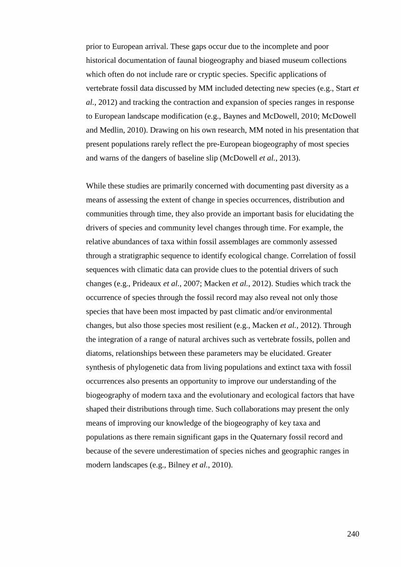
240
prior to European arrival. These gaps occur due to the incomplete and poor
historical documentation of faunal biogeography and biased museum collections
which often do not include rare or cryptic species. Specific applications of
vertebrate fossil data discussed by MM included detecting new species (e.g., Start et
al., 2012) and tracking the contraction and expansion of species ranges in response
to European landscape modification (e.g., Baynes and McDowell, 2010; McDowell
and Medlin, 2010). Drawing on his own research, MM noted in his presentation that
present populations rarely reflect the pre-European biogeography of most species
and warns of the dangers of baseline slip (McDowell et al., 2013).
While these studies are primarily concerned with documenting past diversity as a
means of assessing the extent of change in species occurrences, distribution and
communities through time, they also provide an important basis for elucidating the
drivers of species and community level changes through time. For example, the
relative abundances of taxa within fossil assemblages are commonly assessed
through a stratigraphic sequence to identify ecological change. Correlation of fossil
sequences with climatic data can provide clues to the potential drivers of such
changes (e.g., Prideaux et al., 2007; Macken et al., 2012). Studies which track the
occurrence of species through the fossil record may also reveal not only those
species that have been most impacted by past climatic and/or environmental
changes, but also those species most resilient (e.g., Macken et al., 2012). Through
the integration of a range of natural archives such as vertebrate fossils, pollen and
diatoms, relationships between these parameters may be elucidated. Greater
synthesis of phylogenetic data from living populations and extinct taxa with fossil
occurrences also presents an opportunity to improve our understanding of the
biogeography of modern taxa and the evolutionary and ecological factors that have
shaped their distributions through time. Such collaborations may present the only
means of improving our knowledge of the biogeography of key taxa and
populations as there remain significant gaps in the Quaternary fossil record and
because of the severe underestimation of species niches and geographic ranges in
modern landscapes (e.g., Bilney et al., 2010).
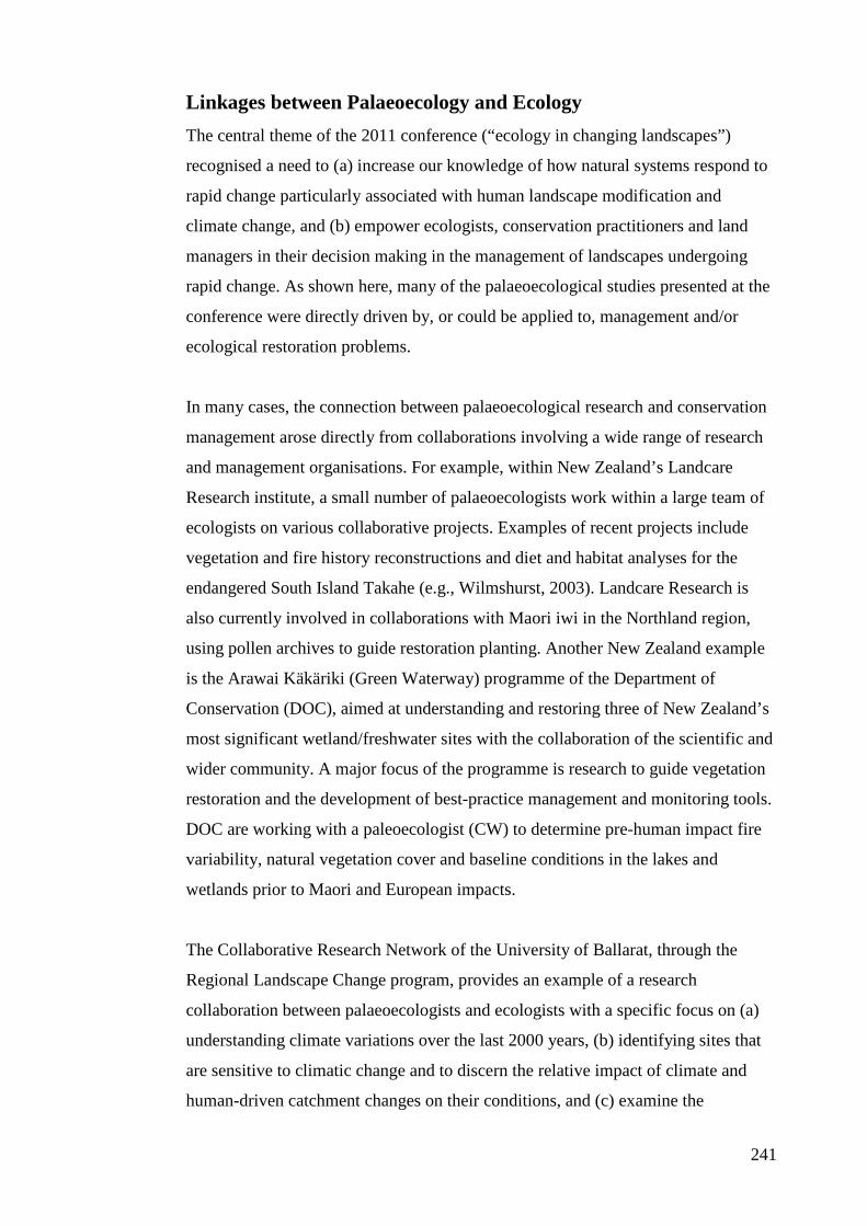
241
Linkages between Palaeoecology and Ecology The central theme of the 2011 conference (“ecology in changing landscapes”)
recognised a need to (a) increase our knowledge of how natural systems respond to
rapid change particularly associated with human landscape modification and
climate change, and (b) empower ecologists, conservation practitioners and land
managers in their decision making in the management of landscapes undergoing
rapid change. As shown here, many of the palaeoecological studies presented at the
conference were directly driven by, or could be applied to, management and/or
ecological restoration problems.
In many cases, the connection between palaeoecological research and conservation
management arose directly from collaborations involving a wide range of research
and management organisations. For example, within New Zealand’s Landcare
Research institute, a small number of palaeoecologists work within a large team of
ecologists on various collaborative projects. Examples of recent projects include
vegetation and fire history reconstructions and diet and habitat analyses for the
endangered South Island Takahe (e.g., Wilmshurst, 2003). Landcare Research is
also currently involved in collaborations with Maori iwi in the Northland region,
using pollen archives to guide restoration planting. Another New Zealand example
is the Arawai Käkäriki (Green Waterway) programme of the Department of
Conservation (DOC), aimed at understanding and restoring three of New Zealand’s
most significant wetland/freshwater sites with the collaboration of the scientific and
wider community. A major focus of the programme is research to guide vegetation
restoration and the development of best-practice management and monitoring tools.
DOC are working with a paleoecologist (CW) to determine pre-human impact fire
variability, natural vegetation cover and baseline conditions in the lakes and
wetlands prior to Maori and European impacts.
The Collaborative Research Network of the University of Ballarat, through the
Regional Landscape Change program, provides an example of a research
collaboration between palaeoecologists and ecologists with a specific focus on (a)
understanding climate variations over the last 2000 years, (b) identifying sites that
are sensitive to climatic change and to discern the relative impact of climate and
human-driven catchment changes on their conditions, and (c) examine the
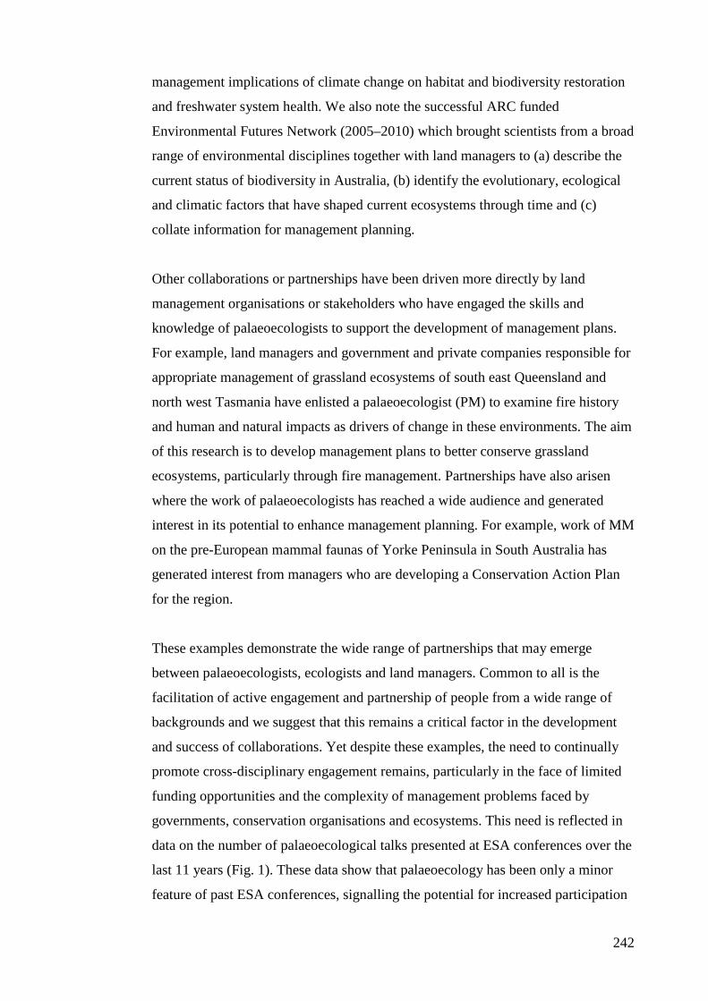
242
management implications of climate change on habitat and biodiversity restoration
and freshwater system health. We also note the successful ARC funded
Environmental Futures Network (2005–2010) which brought scientists from a broad
range of environmental disciplines together with land managers to (a) describe the
current status of biodiversity in Australia, (b) identify the evolutionary, ecological
and climatic factors that have shaped current ecosystems through time and (c)
collate information for management planning.
Other collaborations or partnerships have been driven more directly by land
management organisations or stakeholders who have engaged the skills and
knowledge of palaeoecologists to support the development of management plans.
For example, land managers and government and private companies responsible for
appropriate management of grassland ecosystems of south east Queensland and
north west Tasmania have enlisted a palaeoecologist (PM) to examine fire history
and human and natural impacts as drivers of change in these environments. The aim
of this research is to develop management plans to better conserve grassland
ecosystems, particularly through fire management. Partnerships have also arisen
where the work of palaeoecologists has reached a wide audience and generated
interest in its potential to enhance management planning. For example, work of MM
on the pre-European mammal faunas of Yorke Peninsula in South Australia has
generated interest from managers who are developing a Conservation Action Plan
for the region.
These examples demonstrate the wide range of partnerships that may emerge
between palaeoecologists, ecologists and land managers. Common to all is the
facilitation of active engagement and partnership of people from a wide range of
backgrounds and we suggest that this remains a critical factor in the development
and success of collaborations. Yet despite these examples, the need to continually
promote cross-disciplinary engagement remains, particularly in the face of limited
funding opportunities and the complexity of management problems faced by
governments, conservation organisations and ecosystems. This need is reflected in
data on the number of palaeoecological talks presented at ESA conferences over the
last 11 years (Fig. 1). These data show that palaeoecology has been only a minor
feature of past ESA conferences, signalling the potential for increased participation
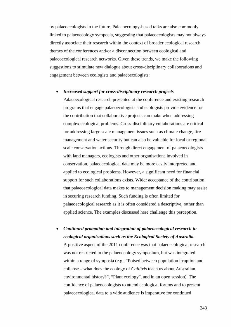
243
by palaeoecologists in the future. Palaeoecology-based talks are also commonly
linked to palaeoecology symposia, suggesting that palaeoecologists may not always
directly associate their research within the context of broader ecological research
themes of the conferences and/or a disconnection between ecological and
palaeoecological research networks. Given these trends, we make the following
suggestions to stimulate new dialogue about cross-disciplinary collaborations and
engagement between ecologists and palaeoecologists:
• Increased support for cross-disciplinary research projects
Palaeoecological research presented at the conference and existing research
programs that engage palaeoecologists and ecologists provide evidence for
the contribution that collaborative projects can make when addressing
complex ecological problems. Cross-disciplinary collaborations are critical
for addressing large scale management issues such as climate change, fire
management and water security but can also be valuable for local or regional
scale conservation actions. Through direct engagement of palaeoecologists
with land managers, ecologists and other organisations involved in
conservation, palaeoecological data may be more easily interpreted and
applied to ecological problems. However, a significant need for financial
support for such collaborations exists. Wider acceptance of the contribution
that palaeoecological data makes to management decision making may assist
in securing research funding. Such funding is often limited for
palaeoecological research as it is often considered a descriptive, rather than
applied science. The examples discussed here challenge this perception.
• Continued promotion and integration of palaeoecological research in
ecological organisations such as the Ecological Society of Australia.
A positive aspect of the 2011 conference was that palaeoecological research
was not restricted to the palaeoecology symposium, but was integrated
within a range of symposia (e.g., “Poised between population irruption and
collapse – what does the ecology of Callitris teach us about Australian
environmental history?”, “Plant ecology”, and in an open session). The
confidence of palaeoecologists to attend ecological forums and to present
palaeoecological data to a wide audience is imperative for continued
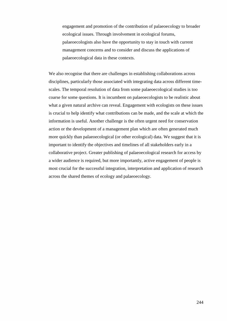
244
engagement and promotion of the contribution of palaeoecology to broader
ecological issues. Through involvement in ecological forums,
palaeoecologists also have the opportunity to stay in touch with current
management concerns and to consider and discuss the applications of
palaeoecological data in these contexts.
We also recognise that there are challenges in establishing collaborations across
disciplines, particularly those associated with integrating data across different time-
scales. The temporal resolution of data from some palaeoecological studies is too
coarse for some questions. It is incumbent on palaeoecologists to be realistic about
what a given natural archive can reveal. Engagement with ecologists on these issues
is crucial to help identify what contributions can be made, and the scale at which the
information is useful. Another challenge is the often urgent need for conservation
action or the development of a management plan which are often generated much
more quickly than palaeoecological (or other ecological) data. We suggest that it is
important to identify the objectives and timelines of all stakeholders early in a
collaborative project. Greater publishing of palaeoecological research for access by
a wider audience is required, but more importantly, active engagement of people is
most crucial for the successful integration, interpretation and application of research
across the shared themes of ecology and palaeoecology.
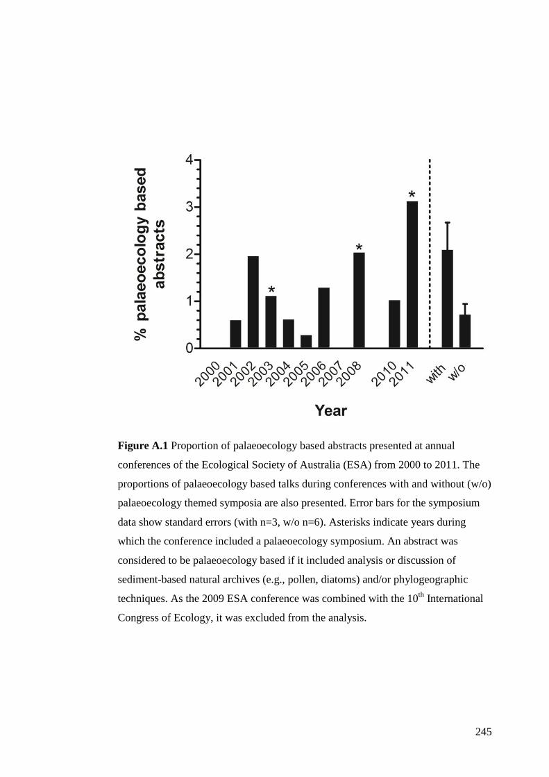
245
Figure A.1 Proportion of palaeoecology based abstracts presented at annual
conferences of the Ecological Society of Australia (ESA) from 2000 to 2011. The
proportions of palaeoecology based talks during conferences with and without (w/o)
palaeoecology themed symposia are also presented. Error bars for the symposium
data show standard errors (with n=3, w/o n=6). Asterisks indicate years during
which the conference included a palaeoecology symposium. An abstract was
considered to be palaeoecology based if it included analysis or discussion of
sediment-based natural archives (e.g., pollen, diatoms) and/or phylogeographic
techniques. As the 2009 ESA conference was combined with the 10th International
Congress of Ecology, it was excluded from the analysis.
246
Conclusion The common research themes between palaeoecological and ecological research
presented at the 2011 ESA conference reflect a high degree of cross-over between
these often separated disciplines. Palaeoecological research presented at the
conference provides examples of the contribution that long-term records can make
to our understanding of natural systems and to our management decision making.
The shared research themes also reflect the importance of current ecological
research and problems faced by land managers in directing palaeoecological
research.
As palaeoecologists, there is inherent value for us in engaging with the ecological
research community and the ESA; in many cases we share the goal of providing
information that can be used to make appropriate and effective decisions for the
conservation of species, landscapes and ecological processes. Continued
engagement of palaeoecology and ecology through the ESA annual conference,
both within and outside of palaeoecology specific symposia, and the development
of research collaborations will strengthen the linkages between our disciplines. As
demonstrated in the examples discussed here, increased participation and
collaboration can also make significant contributions to informed and appropriate
ecosystem management and restoration.
Acknowledgements We extend our thanks to the Ecological Society of Australia and the 2011
conference organising committee for facilitating engagement between
palaeoecologists and ecologists at the 2011 annual meeting. We also acknowledge
palaeoecologists who attended the 2011 conference, but who were not able to
contribute directly to the manuscript.
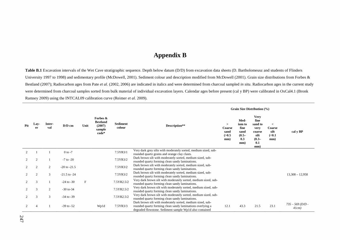
247
Appendix B
Table B.1 Excavation intervals of the Wet Cave stratigraphic sequence. Depth below datum (D/D) from excavation data sheets (D. Bartholomeusz and students of Flinders
University 1997 to 1998) and sedimentary profile (McDowell, 2001). Sediment colour and description modified from McDowell (2001). Grain size distributions from Forbes &
Bestland (2007); Radiocarbon ages from Pate et al. (2002, 2006) are indicated in italics and were determined from charcoal sampled in situ. Radiocarbon ages in the current study
were determined from charcoal samples sorted from bulk material of individual excavation layers. Calendar ages before present (cal y BP) were calibrated in OxCal4.1 (Bronk
Ramsey 2009) using the INTCAL09 calibration curve (Reimer et al. 2009).
Pit Lay-er
Inter-val D/D cm Unit
Forbes & Bestland
(2007) sample code*
Sediment colour Description**
Grain Size Distribution (%)
> Coarse
sand (>0.5 mm)
Med-ium to
fine sand (0.5–0.3
mm)
Very fine
sand to very
coarse silt
(0.3–0.1
mm)
< Coarse
silt (<0.1 mm)
cal y BP
2 1 1 0 to -7 7.5YR3/1 Very dark grey silts with moderately sorted, medium sized, sub-rounded quartz grains and orange clay clasts.
2 2 1 -7 to -20 7.5YR3/2 Dark brown silt with moderately sorted, medium sized, sub-rounded quartz forming clean sandy laminations.
2 2 2 -20 to -21.5 7.5YR3/2 Dark brown silt with moderately sorted, medium sized, sub-rounded quartz forming clean sandy laminations.
2 2 3 -21.5 to -24 7.5YR3/2 Dark brown silt with moderately sorted, medium sized, sub-rounded quartz forming clean sandy laminations. 13,308 – 12,958
2 3 1 -24 to -30 F 7.5YR2.5/2 Very dark brown silt with moderately sorted, medium sized, sub-rounded quartz forming clean sandy laminations.
2 3 2 -30 to-34 7.5YR2.5/2 Very dark brown silt with moderately sorted, medium sized, sub-rounded quartz forming clean sandy laminations.
2 3 3 -34 to -39 7.5YR2.5/2 Very dark brown silt with moderately sorted, medium sized, sub-rounded quartz forming clean sandy laminations.
2 4 1 -39 to -52
Wp1d 7.5YR3/3 Dark brown silt with moderately sorted, medium sized, sub-rounded quartz forming clean sandy laminations overlying a degraded flowstone. Sediment sample Wp1d also contained
12.1 43.3 21.5 23.1 735 – 569 (D/D -41cm)
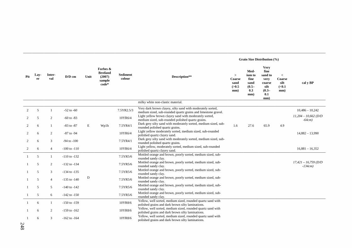
248
Pit Lay-er
Inter-val D/D cm Unit
Forbes & Bestland
(2007) sample code*
Sediment colour Description**
Grain Size Distribution (%)
> Coarse
sand (>0.5 mm)
Med-ium to
fine sand (0.5–0.3
mm)
Very fine
sand to very
coarse silt
(0.3–0.1
mm)
< Coarse
silt (<0.1 mm)
cal y BP
milky white non-clastic material.
2 5 1 -52 to -60 7.5YR2.5/3 Very dark brown clayey, silty sand with moderately sorted, medium sized, sub-rounded quartz grains and limestone gravel. 10,486 – 10,242
2 5 2 -60 to -83 10YR6/4 Light yellow brown clayey sand with moderately sorted, medium sized, sub-rounded polished quartz grains. 11,204 – 10,662 (D/D
-64cm)
2 6 1 -83 to -87 E Wp1h 7.5YR4/1 Dark grey silty sand with moderately sorted, medium sized, sub-rounded polished quartz grains. 1.6 27.6 65.9 4.9
2 6 2 -87 to -94 10YR6/4 Light yellow moderately sorted, medium sized, sub-rounded polished quartz clayey sand. 14,882 – 13,990
2 6 3 -94 to -100 7.5YR4/1 Dark grey silty sand with moderately sorted, medium sized, sub-rounded polished quartz grains.
2 6 4 -100 to -110 10YR6/4 Light yellow, moderately sorted, medium sized, sub-rounded polished quartz clayey sand. 16,881 – 16,352
1 5 1 -110 to -132 7.5YR5/6 Mottled orange and brown, poorly sorted, medium sized, sub-rounded sandy clay.
1 5 2 -132 to -134 7.5YR5/6 Mottled orange and brown, poorly sorted, medium sized, sub-rounded sandy clay. 17,421 – 16,759 (D/D
-134cm)
1 5 3 -134 to -135 7.5YR5/6 Mottled orange and brown, poorly sorted, medium sized, sub-rounded sandy clay.
1 5 4 -135 to -140 D 7.5YR5/6 Mottled orange and brown, poorly sorted, medium sized, sub-rounded sandy clay.
1 5 5 -140 to -142 7.5YR5/6 Mottled orange and brown, poorly sorted, medium sized, sub-rounded sandy clay.
1 5 6 -142 to -150 7.5YR5/6 Mottled orange and brown, poorly sorted, medium sized, sub-rounded sandy clay.
1 6 1 -150 to -159 10YR8/6 Yellow, well sorted, medium sized, rounded quartz sand with polished grains and dark brown silty laminations.
1 6 2 -159 to -162 10YR8/6 Yellow, well sorted, medium sized, rounded quartz sand with polished grains and dark brown silty laminations.
1 6 3 -162 to -164 10YR8/6 Yellow, well sorted, medium sized, rounded quartz sand with polished grains and dark brown silty laminations.
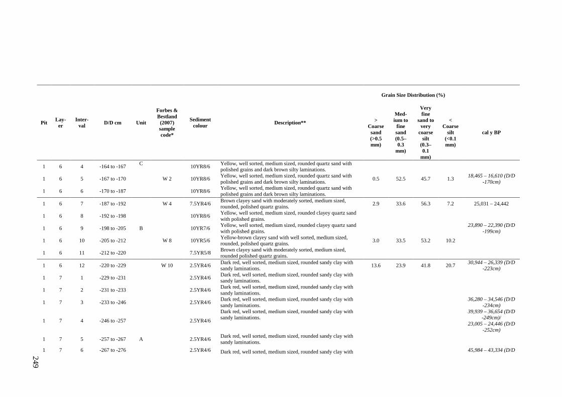
249
Pit Lay-er
Inter-val D/D cm Unit
Forbes & Bestland
(2007) sample code*
Sediment colour Description**
Grain Size Distribution (%)
> Coarse
sand (>0.5 mm)
Med-ium to
fine sand (0.5–0.3
mm)
Very fine
sand to very
coarse silt
(0.3–0.1
mm)
< Coarse
silt (<0.1 mm)
cal y BP
1 6 4 -164 to -167 C 10YR8/6 Yellow, well sorted, medium sized, rounded quartz sand with polished grains and dark brown silty laminations.
1 6 5 -167 to -170 W 2 10YR8/6 Yellow, well sorted, medium sized, rounded quartz sand with polished grains and dark brown silty laminations. 0.5 52.5 45.7 1.3 18,465 – 16,610 (D/D
-170cm)
1 6 6 -170 to -187 10YR8/6 Yellow, well sorted, medium sized, rounded quartz sand with polished grains and dark brown silty laminations.
1 6 7 -187 to -192 W 4 7.5YR4/6 Brown clayey sand with moderately sorted, medium sized, rounded, polished quartz grains. 2.9 33.6 56.3 7.2 25,031 – 24,442
1 6 8 -192 to -198 10YR8/6 Yellow, well sorted, medium sized, rounded clayey quartz sand with polished grains.
1 6 9 -198 to -205 B 10YR7/6 Yellow, well sorted, medium sized, rounded clayey quartz sand with polished grains. 23,890 – 22,390 (D/D
-199cm)
1 6 10 -205 to -212 W 8 10YR5/6 Yellow-brown clayey sand with well sorted, medium sized, rounded, polished quartz grains. 3.0 33.5 53.2 10.2
1 6 11 -212 to -220 7.5YR5/8 Brown clayey sand with moderately sorted, medium sized, rounded polished quartz grains.
1 6 12 -220 to -229 W 10 2.5YR4/6 Dark red, well sorted, medium sized, rounded sandy clay with sandy laminations. 13.6 23.9 41.8 20.7 30,944 – 26,339 (D/D
-223cm)
1 7 1 -229 to -231 2.5YR4/6 Dark red, well sorted, medium sized, rounded sandy clay with sandy laminations.
1 7 2 -231 to -233 2.5YR4/6 Dark red, well sorted, medium sized, rounded sandy clay with sandy laminations.
1 7 3 -233 to -246 2.5YR4/6 Dark red, well sorted, medium sized, rounded sandy clay with sandy laminations. 36,280 – 34,546 (D/D
-234cm)
1 7 4 -246 to -257 2.5YR4/6
Dark red, well sorted, medium sized, rounded sandy clay with sandy laminations.
39,939 – 36,654 (D/D -249cm)/
23,005 – 24,446 (D/D -252cm)
1 7 5 -257 to -267 A 2.5YR4/6 Dark red, well sorted, medium sized, rounded sandy clay with sandy laminations.
1 7 6 -267 to -276 2.5YR4/6 Dark red, well sorted, medium sized, rounded sandy clay with 45,984 – 43,334 (D/D
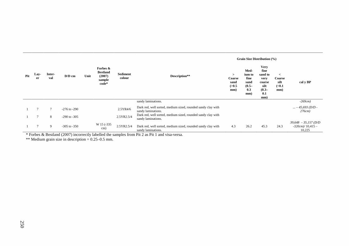
250
Pit Lay-er
Inter-val D/D cm Unit
Forbes & Bestland
(2007) sample code*
Sediment colour Description**
Grain Size Distribution (%)
> Coarse
sand (>0.5 mm)
Med-ium to
fine sand (0.5–0.3
mm)
Very fine
sand to very
coarse silt
(0.3–0.1
mm)
< Coarse
silt (<0.1 mm)
cal y BP
sandy laminations. -269cm)
1 7 7 -276 to -290 2.5YR4/6 Dark red, well sorted, medium sized, rounded sandy clay with sandy laminations. ... – 45,693 (D/D -
276cm)
1 7 8 -290 to -305 2.5YR2.5/4 Dark red, well sorted, medium sized, rounded sandy clay with sandy laminations.
1 7 9 -305 to -350 W 15 (-335
cm) 2.5YR2.5/4 Dark red, well sorted, medium sized, rounded sandy clay with sandy laminations.
4.3 26.2 45.3 24.3 39,648 – 35,157 (D/D
-320cm)/ 10,415 – 10,225
* Forbes & Bestland (2007) incorrectly labelled the samples from Pit 2 as Pit 1 and visa-versa. ** Medium grain size in description = 0.25–0.5 mm.
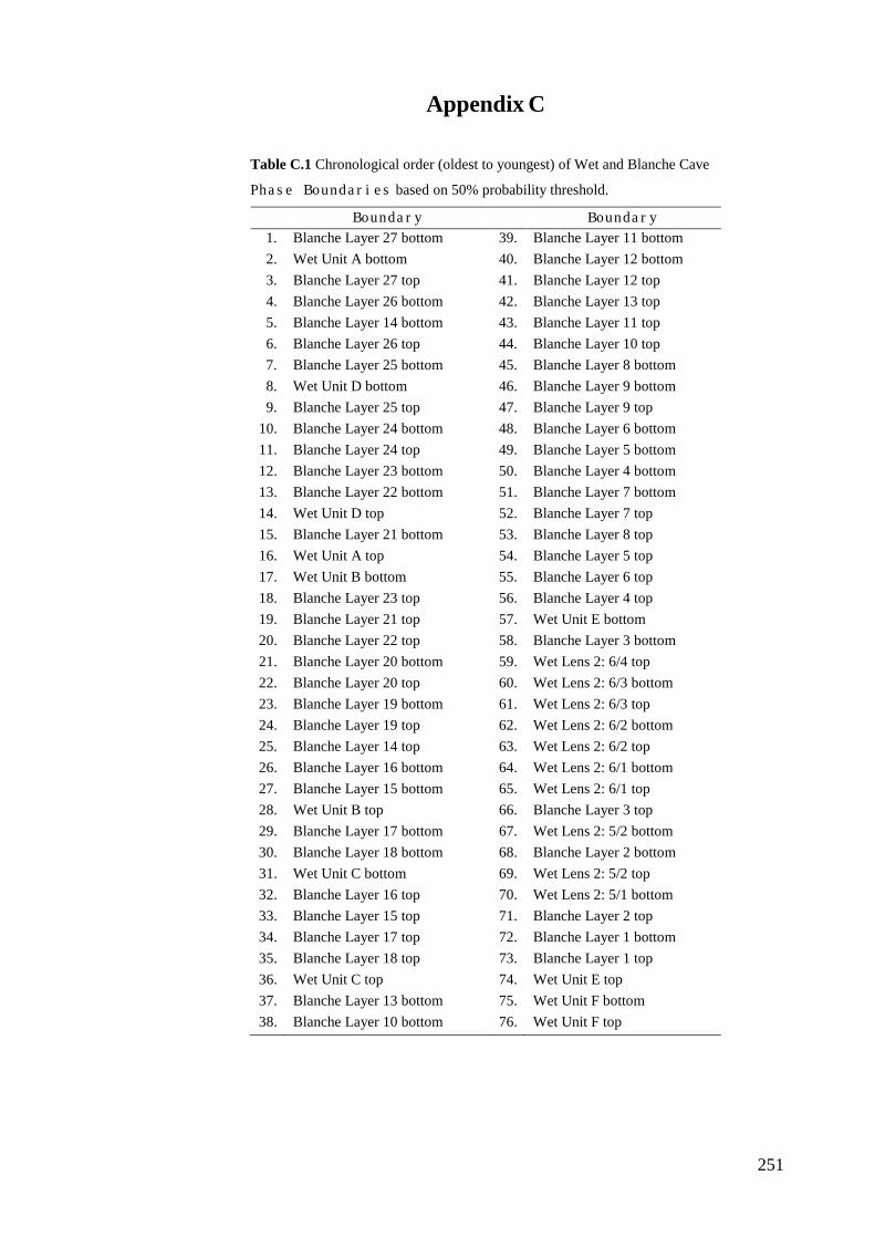
251
Appendix C
Table C.1 Chronological order (oldest to youngest) of Wet and Blanche Cave
Phase Boundaries based on 50% probability threshold.
Boundary Boundary
1. Blanche Layer 27 bottom 39. Blanche Layer 11 bottom 2. Wet Unit A bottom 40. Blanche Layer 12 bottom 3. Blanche Layer 27 top 41. Blanche Layer 12 top 4. Blanche Layer 26 bottom 42. Blanche Layer 13 top 5. Blanche Layer 14 bottom 43. Blanche Layer 11 top 6. Blanche Layer 26 top 44. Blanche Layer 10 top 7. Blanche Layer 25 bottom 45. Blanche Layer 8 bottom 8. Wet Unit D bottom 46. Blanche Layer 9 bottom 9. Blanche Layer 25 top 47. Blanche Layer 9 top
10. Blanche Layer 24 bottom 48. Blanche Layer 6 bottom 11. Blanche Layer 24 top 49. Blanche Layer 5 bottom 12. Blanche Layer 23 bottom 50. Blanche Layer 4 bottom 13. Blanche Layer 22 bottom 51. Blanche Layer 7 bottom 14. Wet Unit D top 52. Blanche Layer 7 top 15. Blanche Layer 21 bottom 53. Blanche Layer 8 top 16. Wet Unit A top 54. Blanche Layer 5 top 17. Wet Unit B bottom 55. Blanche Layer 6 top 18. Blanche Layer 23 top 56. Blanche Layer 4 top 19. Blanche Layer 21 top 57. Wet Unit E bottom 20. Blanche Layer 22 top 58. Blanche Layer 3 bottom 21. Blanche Layer 20 bottom 59. Wet Lens 2: 6/4 top 22. Blanche Layer 20 top 60. Wet Lens 2: 6/3 bottom 23. Blanche Layer 19 bottom 61. Wet Lens 2: 6/3 top 24. Blanche Layer 19 top 62. Wet Lens 2: 6/2 bottom 25. Blanche Layer 14 top 63. Wet Lens 2: 6/2 top 26. Blanche Layer 16 bottom 64. Wet Lens 2: 6/1 bottom 27. Blanche Layer 15 bottom 65. Wet Lens 2: 6/1 top 28. Wet Unit B top 66. Blanche Layer 3 top 29. Blanche Layer 17 bottom 67. Wet Lens 2: 5/2 bottom 30. Blanche Layer 18 bottom 68. Blanche Layer 2 bottom 31. Wet Unit C bottom 69. Wet Lens 2: 5/2 top 32. Blanche Layer 16 top 70. Wet Lens 2: 5/1 bottom 33. Blanche Layer 15 top 71. Blanche Layer 2 top 34. Blanche Layer 17 top 72. Blanche Layer 1 bottom 35. Blanche Layer 18 top 73. Blanche Layer 1 top 36. Wet Unit C top 74. Wet Unit E top 37. Blanche Layer 13 bottom 75. Wet Unit F bottom 38. Blanche Layer 10 bottom 76. Wet Unit F top
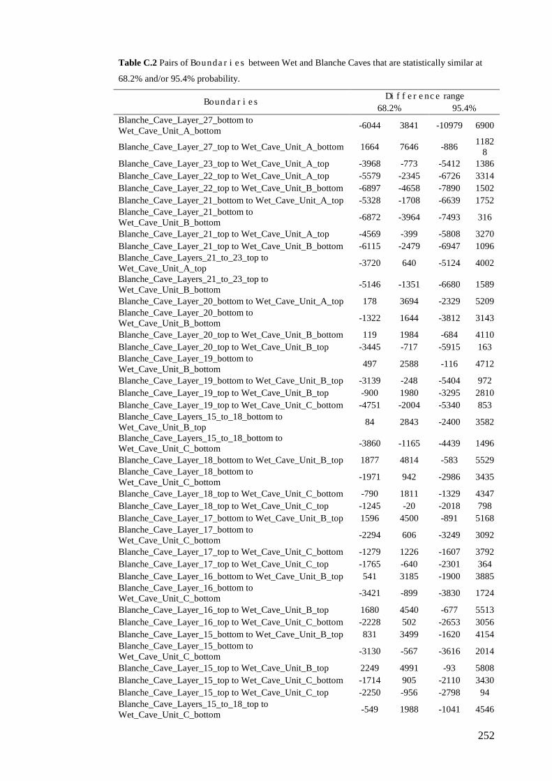
252
Table C.2 Pairs of Boundaries between Wet and Blanche Caves that are statistically similar at
68.2% and/or 95.4% probability.
Boundaries Difference range 68.2% 95.4%
Blanche_Cave_Layer_27_bottom to Wet_Cave_Unit_A_bottom -6044 3841 -10979 6900
Blanche_Cave_Layer_27_top to Wet_Cave_Unit_A_bottom 1664 7646 -886 11828
Blanche_Cave_Layer_23_top to Wet_Cave_Unit_A_top -3968 -773 -5412 1386 Blanche_Cave_Layer_22_top to Wet_Cave_Unit_A_top -5579 -2345 -6726 3314 Blanche_Cave_Layer_22_top to Wet_Cave_Unit_B_bottom -6897 -4658 -7890 1502 Blanche_Cave_Layer_21_bottom to Wet_Cave_Unit_A_top -5328 -1708 -6639 1752 Blanche_Cave_Layer_21_bottom to Wet_Cave_Unit_B_bottom -6872 -3964 -7493 316
Blanche_Cave_Layer_21_top to Wet_Cave_Unit_A_top -4569 -399 -5808 3270 Blanche_Cave_Layer_21_top to Wet_Cave_Unit_B_bottom -6115 -2479 -6947 1096 Blanche_Cave_Layers_21_to_23_top to Wet_Cave_Unit_A_top -3720 640 -5124 4002
Blanche_Cave_Layers_21_to_23_top to Wet_Cave_Unit_B_bottom -5146 -1351 -6680 1589
Blanche_Cave_Layer_20_bottom to Wet_Cave_Unit_A_top 178 3694 -2329 5209 Blanche_Cave_Layer_20_bottom to Wet_Cave_Unit_B_bottom -1322 1644 -3812 3143
Blanche_Cave_Layer_20_top to Wet_Cave_Unit_B_bottom 119 1984 -684 4110 Blanche_Cave_Layer_20_top to Wet_Cave_Unit_B_top -3445 -717 -5915 163 Blanche_Cave_Layer_19_bottom to Wet_Cave_Unit_B_bottom 497 2588 -116 4712
Blanche_Cave_Layer_19_bottom to Wet_Cave_Unit_B_top -3139 -248 -5404 972 Blanche_Cave_Layer_19_top to Wet_Cave_Unit_B_top -900 1980 -3295 2810 Blanche_Cave_Layer_19_top to Wet_Cave_Unit_C_bottom -4751 -2004 -5340 853 Blanche_Cave_Layers_15_to_18_bottom to Wet_Cave_Unit_B_top 84 2843 -2400 3582
Blanche_Cave_Layers_15_to_18_bottom to Wet_Cave_Unit_C_bottom -3860 -1165 -4439 1496
Blanche_Cave_Layer_18_bottom to Wet_Cave_Unit_B_top 1877 4814 -583 5529 Blanche_Cave_Layer_18_bottom to Wet_Cave_Unit_C_bottom -1971 942 -2986 3435
Blanche_Cave_Layer_18_top to Wet_Cave_Unit_C_bottom -790 1811 -1329 4347 Blanche_Cave_Layer_18_top to Wet_Cave_Unit_C_top -1245 -20 -2018 798 Blanche_Cave_Layer_17_bottom to Wet_Cave_Unit_B_top 1596 4500 -891 5168 Blanche_Cave_Layer_17_bottom to Wet_Cave_Unit_C_bottom -2294 606 -3249 3092
Blanche_Cave_Layer_17_top to Wet_Cave_Unit_C_bottom -1279 1226 -1607 3792 Blanche_Cave_Layer_17_top to Wet_Cave_Unit_C_top -1765 -640 -2301 364 Blanche_Cave_Layer_16_bottom to Wet_Cave_Unit_B_top 541 3185 -1900 3885 Blanche_Cave_Layer_16_bottom to Wet_Cave_Unit_C_bottom -3421 -899 -3830 1724
Blanche_Cave_Layer_16_top to Wet_Cave_Unit_B_top 1680 4540 -677 5513 Blanche_Cave_Layer_16_top to Wet_Cave_Unit_C_bottom -2228 502 -2653 3056 Blanche_Cave_Layer_15_bottom to Wet_Cave_Unit_B_top 831 3499 -1620 4154 Blanche_Cave_Layer_15_bottom to Wet_Cave_Unit_C_bottom -3130 -567 -3616 2014
Blanche_Cave_Layer_15_top to Wet_Cave_Unit_B_top 2249 4991 -93 5808 Blanche_Cave_Layer_15_top to Wet_Cave_Unit_C_bottom -1714 905 -2110 3430 Blanche_Cave_Layer_15_top to Wet_Cave_Unit_C_top -2250 -956 -2798 94 Blanche_Cave_Layers_15_to_18_top to Wet_Cave_Unit_C_bottom -549 1988 -1041 4546
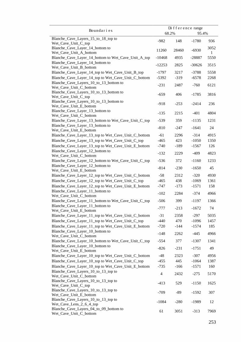
253
Boundaries Difference range 68.2% 95.4%
Blanche_Cave_Layers_15_to_18_top to Wet_Cave_Unit_C_top -982 148 -1780 936
Blanche_Cave_Layer_14_bottom to Wet_Cave_Unit_A_bottom 11260 28460 -6930 3052
1 Blanche_Cave_Layer_14_bottom to Wet_Cave_Unit_A_top -10468 4935 -28887 5550 Blanche_Cave_Layer_14_bottom to Wet_Cave_Unit_B_bottom -12253 2825 -30626 3515
Blanche_Cave_Layer_14_top to Wet_Cave_Unit_B_top -1797 3217 -3788 5558 Blanche_Cave_Layer_14_top to Wet_Cave_Unit_C_bottom -5392 -319 -6578 2268 Blanche_Cave_Layers_10_to_13_bottom to Wet_Cave_Unit_C_bottom -231 2487 -760 6121
Blanche_Cave_Layers_10_to_13_bottom to Wet_Cave_Unit_C_top -659 406 -1785 3816
Blanche_Cave_Layers_10_to_13_bottom to Wet_Cave_Unit_E_bottom -918 -253 -2414 236
Blanche_Cave_Layer_13_bottom to Wet_Cave_Unit_C_bottom -135 2215 -401 4804
Blanche_Cave_Layer_13_bottom to Wet_Cave_Unit_C_top -539 359 -1135 1231 Blanche_Cave_Layer_13_bottom to Wet_Cave_Unit_E_bottom -810 -247 -1641 24
Blanche_Cave_Layer_13_top to Wet_Cave_Unit_C_bottom -61 2296 -314 4915 Blanche_Cave_Layer_13_top to Wet_Cave_Unit_C_top -465 423 -1050 1350 Blanche_Cave_Layer_13_top to Wet_Cave_Unit_E_bottom -740 -189 -1567 126 Blanche_Cave_Layer_12_bottom to Wet_Cave_Unit_C_bottom -132 2229 -409 4823
Blanche_Cave_Layer_12_bottom to Wet_Cave_Unit_C_top -536 372 -1160 1233 Blanche_Cave_Layer_12_bottom to Wet_Cave_Unit_E_bottom -814 -230 -1650 45
Blanche_Cave_Layer_12_top to Wet_Cave_Unit_C_bottom -58 2312 -320 4930 Blanche_Cave_Layer_12_top to Wet_Cave_Unit_C_top -465 438 -1069 1361 Blanche_Cave_Layer_12_top to Wet_Cave_Unit_E_bottom -747 -173 -1571 158 Blanche_Cave_Layer_11_bottom to Wet_Cave_Unit_C_bottom -102 2284 -374 4966
Blanche_Cave_Layer_11_bottom to Wet_Cave_Unit_C_top -506 399 -1197 1366 Blanche_Cave_Layer_11_bottom to Wet_Cave_Unit_E_bottom -777 -213 -1672 74
Blanche_Cave_Layer_11_top to Wet_Cave_Unit_C_bottom -31 2358 -297 5035 Blanche_Cave_Layer_11_top to Wet_Cave_Unit_C_top -440 470 -1096 1457 Blanche_Cave_Layer_11_top to Wet_Cave_Unit_E_bottom -720 -144 -1574 185 Blanche_Cave_Layer_10_bottom to Wet_Cave_Unit_C_bottom -148 2262 -445 4966
Blanche_Cave_Layer_10_bottom to Wet_Cave_Unit_C_top -554 377 -1307 1341 Blanche_Cave_Layer_10_bottom to Wet_Cave_Unit_E_bottom -826 -231 -1751 49
Blanche_Cave_Layer_10_top to Wet_Cave_Unit_C_bottom -48 2323 -307 4956 Blanche_Cave_Layer_10_top to Wet_Cave_Unit_C_top -455 445 -1064 1387 Blanche_Cave_Layer_10_top to Wet_Cave_Unit_E_bottom -735 -166 -1571 160 Blanche_Cave_Layers_10_to_13_top to Wet_Cave_Unit_C_bottom 4 2432 -275 5170
Blanche_Cave_Layers_10_to_13_top to Wet_Cave_Unit_C_top -413 529 -1150 1625
Blanche_Cave_Layers_10_to_13_top to Wet_Cave_Unit_E_bottom -709 -89 -1592 307
Blanche_Cave_Layers_10_to_13_top to Wet_Cave_Lens_2_6_4_top -1084 -280 -1989 12
Blanche_Cave_Layers_04_to_09_bottom to Wet_Cave_Unit_C_bottom 61 3051 -313 7969
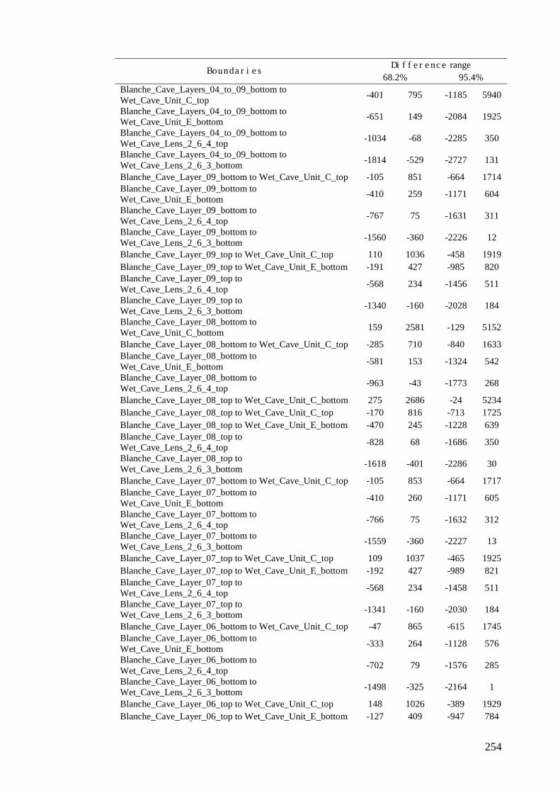
254
Boundaries Difference range 68.2% 95.4%
Blanche_Cave_Layers_04_to_09_bottom to Wet_Cave_Unit_C_top -401 795 -1185 5940
Blanche_Cave_Layers_04_to_09_bottom to Wet_Cave_Unit_E_bottom -651 149 -2084 1925
Blanche_Cave_Layers_04_to_09_bottom to Wet_Cave_Lens_2_6_4_top -1034 -68 -2285 350
Blanche_Cave_Layers_04_to_09_bottom to Wet_Cave_Lens_2_6_3_bottom -1814 -529 -2727 131
Blanche_Cave_Layer_09_bottom to Wet_Cave_Unit_C_top -105 851 -664 1714 Blanche_Cave_Layer_09_bottom to Wet_Cave_Unit_E_bottom -410 259 -1171 604
Blanche_Cave_Layer_09_bottom to Wet_Cave_Lens_2_6_4_top -767 75 -1631 311
Blanche_Cave_Layer_09_bottom to Wet_Cave_Lens_2_6_3_bottom -1560 -360 -2226 12
Blanche_Cave_Layer_09_top to Wet_Cave_Unit_C_top 110 1036 -458 1919 Blanche_Cave_Layer_09_top to Wet_Cave_Unit_E_bottom -191 427 -985 820 Blanche_Cave_Layer_09_top to Wet_Cave_Lens_2_6_4_top -568 234 -1456 511
Blanche_Cave_Layer_09_top to Wet_Cave_Lens_2_6_3_bottom -1340 -160 -2028 184
Blanche_Cave_Layer_08_bottom to Wet_Cave_Unit_C_bottom 159 2581 -129 5152
Blanche_Cave_Layer_08_bottom to Wet_Cave_Unit_C_top -285 710 -840 1633 Blanche_Cave_Layer_08_bottom to Wet_Cave_Unit_E_bottom -581 153 -1324 542
Blanche_Cave_Layer_08_bottom to Wet_Cave_Lens_2_6_4_top -963 -43 -1773 268
Blanche_Cave_Layer_08_top to Wet_Cave_Unit_C_bottom 275 2686 -24 5234 Blanche_Cave_Layer_08_top to Wet_Cave_Unit_C_top -170 816 -713 1725 Blanche_Cave_Layer_08_top to Wet_Cave_Unit_E_bottom -470 245 -1228 639 Blanche_Cave_Layer_08_top to Wet_Cave_Lens_2_6_4_top -828 68 -1686 350
Blanche_Cave_Layer_08_top to Wet_Cave_Lens_2_6_3_bottom -1618 -401 -2286 30
Blanche_Cave_Layer_07_bottom to Wet_Cave_Unit_C_top -105 853 -664 1717 Blanche_Cave_Layer_07_bottom to Wet_Cave_Unit_E_bottom -410 260 -1171 605
Blanche_Cave_Layer_07_bottom to Wet_Cave_Lens_2_6_4_top -766 75 -1632 312
Blanche_Cave_Layer_07_bottom to Wet_Cave_Lens_2_6_3_bottom -1559 -360 -2227 13
Blanche_Cave_Layer_07_top to Wet_Cave_Unit_C_top 109 1037 -465 1925 Blanche_Cave_Layer_07_top to Wet_Cave_Unit_E_bottom -192 427 -989 821 Blanche_Cave_Layer_07_top to Wet_Cave_Lens_2_6_4_top -568 234 -1458 511
Blanche_Cave_Layer_07_top to Wet_Cave_Lens_2_6_3_bottom -1341 -160 -2030 184
Blanche_Cave_Layer_06_bottom to Wet_Cave_Unit_C_top -47 865 -615 1745 Blanche_Cave_Layer_06_bottom to Wet_Cave_Unit_E_bottom -333 264 -1128 576
Blanche_Cave_Layer_06_bottom to Wet_Cave_Lens_2_6_4_top -702 79 -1576 285
Blanche_Cave_Layer_06_bottom to Wet_Cave_Lens_2_6_3_bottom -1498 -325 -2164 1
Blanche_Cave_Layer_06_top to Wet_Cave_Unit_C_top 148 1026 -389 1929 Blanche_Cave_Layer_06_top to Wet_Cave_Unit_E_bottom -127 409 -947 784
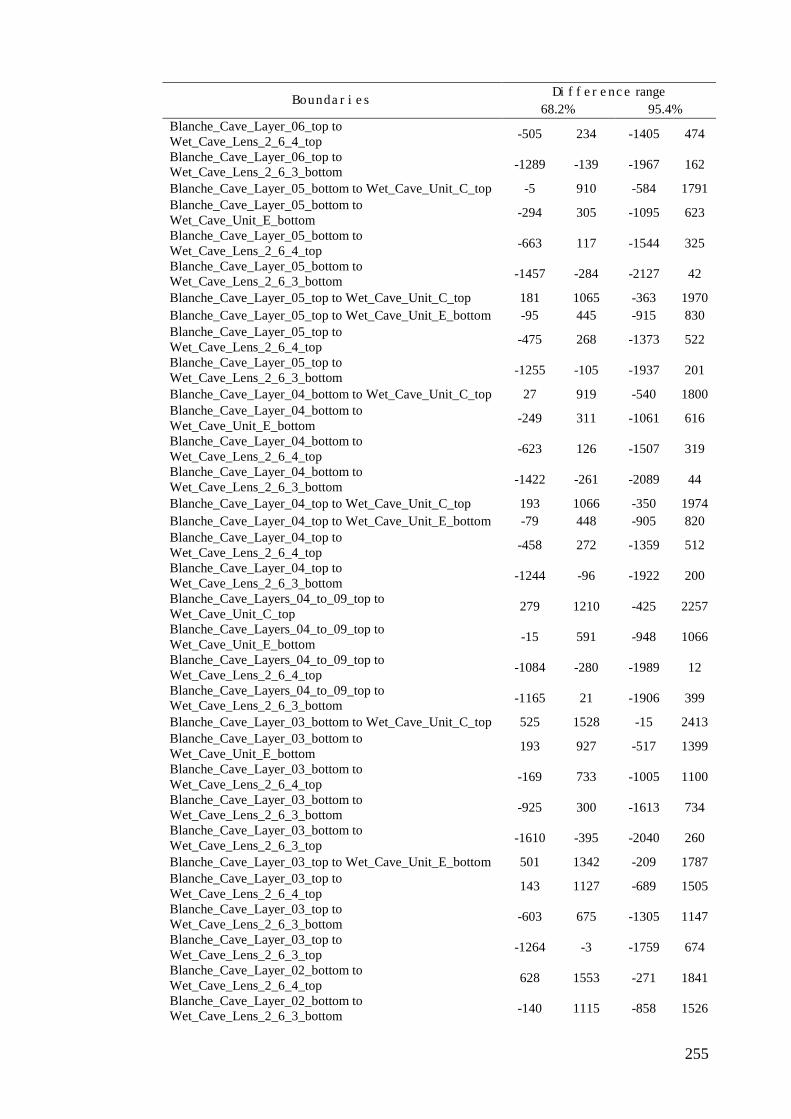
255
Boundaries Difference range 68.2% 95.4%
Blanche_Cave_Layer_06_top to Wet_Cave_Lens_2_6_4_top -505 234 -1405 474
Blanche_Cave_Layer_06_top to Wet_Cave_Lens_2_6_3_bottom -1289 -139 -1967 162
Blanche_Cave_Layer_05_bottom to Wet_Cave_Unit_C_top -5 910 -584 1791 Blanche_Cave_Layer_05_bottom to Wet_Cave_Unit_E_bottom -294 305 -1095 623
Blanche_Cave_Layer_05_bottom to Wet_Cave_Lens_2_6_4_top -663 117 -1544 325
Blanche_Cave_Layer_05_bottom to Wet_Cave_Lens_2_6_3_bottom -1457 -284 -2127 42
Blanche_Cave_Layer_05_top to Wet_Cave_Unit_C_top 181 1065 -363 1970 Blanche_Cave_Layer_05_top to Wet_Cave_Unit_E_bottom -95 445 -915 830 Blanche_Cave_Layer_05_top to Wet_Cave_Lens_2_6_4_top -475 268 -1373 522
Blanche_Cave_Layer_05_top to Wet_Cave_Lens_2_6_3_bottom -1255 -105 -1937 201
Blanche_Cave_Layer_04_bottom to Wet_Cave_Unit_C_top 27 919 -540 1800 Blanche_Cave_Layer_04_bottom to Wet_Cave_Unit_E_bottom -249 311 -1061 616
Blanche_Cave_Layer_04_bottom to Wet_Cave_Lens_2_6_4_top -623 126 -1507 319
Blanche_Cave_Layer_04_bottom to Wet_Cave_Lens_2_6_3_bottom -1422 -261 -2089 44
Blanche_Cave_Layer_04_top to Wet_Cave_Unit_C_top 193 1066 -350 1974 Blanche_Cave_Layer_04_top to Wet_Cave_Unit_E_bottom -79 448 -905 820 Blanche_Cave_Layer_04_top to Wet_Cave_Lens_2_6_4_top -458 272 -1359 512
Blanche_Cave_Layer_04_top to Wet_Cave_Lens_2_6_3_bottom -1244 -96 -1922 200
Blanche_Cave_Layers_04_to_09_top to Wet_Cave_Unit_C_top 279 1210 -425 2257
Blanche_Cave_Layers_04_to_09_top to Wet_Cave_Unit_E_bottom -15 591 -948 1066
Blanche_Cave_Layers_04_to_09_top to Wet_Cave_Lens_2_6_4_top -1084 -280 -1989 12
Blanche_Cave_Layers_04_to_09_top to Wet_Cave_Lens_2_6_3_bottom -1165 21 -1906 399
Blanche_Cave_Layer_03_bottom to Wet_Cave_Unit_C_top 525 1528 -15 2413 Blanche_Cave_Layer_03_bottom to Wet_Cave_Unit_E_bottom 193 927 -517 1399
Blanche_Cave_Layer_03_bottom to Wet_Cave_Lens_2_6_4_top -169 733 -1005 1100
Blanche_Cave_Layer_03_bottom to Wet_Cave_Lens_2_6_3_bottom -925 300 -1613 734
Blanche_Cave_Layer_03_bottom to Wet_Cave_Lens_2_6_3_top -1610 -395 -2040 260
Blanche_Cave_Layer_03_top to Wet_Cave_Unit_E_bottom 501 1342 -209 1787 Blanche_Cave_Layer_03_top to Wet_Cave_Lens_2_6_4_top 143 1127 -689 1505
Blanche_Cave_Layer_03_top to Wet_Cave_Lens_2_6_3_bottom -603 675 -1305 1147
Blanche_Cave_Layer_03_top to Wet_Cave_Lens_2_6_3_top -1264 -3 -1759 674
Blanche_Cave_Layer_02_bottom to Wet_Cave_Lens_2_6_4_top 628 1553 -271 1841
Blanche_Cave_Layer_02_bottom to Wet_Cave_Lens_2_6_3_bottom -140 1115 -858 1526
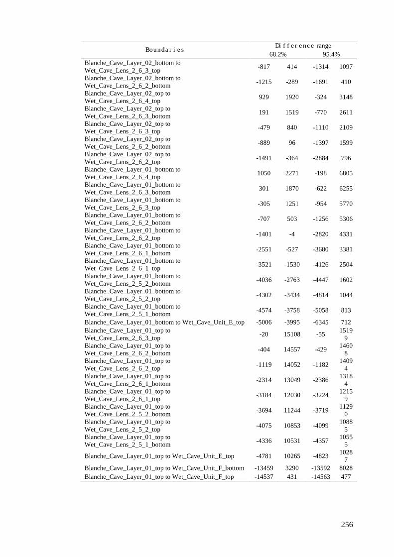
256
Boundaries Difference range 68.2% 95.4%
Blanche_Cave_Layer_02_bottom to Wet_Cave_Lens_2_6_3_top -817 414 -1314 1097
Blanche_Cave_Layer_02_bottom to Wet_Cave_Lens_2_6_2_bottom -1215 -289 -1691 410
Blanche_Cave_Layer_02_top to Wet_Cave_Lens_2_6_4_top 929 1920 -324 3148
Blanche_Cave_Layer_02_top to Wet_Cave_Lens_2_6_3_bottom 191 1519 -770 2611
Blanche_Cave_Layer_02_top to Wet_Cave_Lens_2_6_3_top -479 840 -1110 2109
Blanche_Cave_Layer_02_top to Wet_Cave_Lens_2_6_2_bottom -889 96 -1397 1599
Blanche_Cave_Layer_02_top to Wet_Cave_Lens_2_6_2_top -1491 -364 -2884 796
Blanche_Cave_Layer_01_bottom to Wet_Cave_Lens_2_6_4_top 1050 2271 -198 6805
Blanche_Cave_Layer_01_bottom to Wet_Cave_Lens_2_6_3_bottom 301 1870 -622 6255
Blanche_Cave_Layer_01_bottom to Wet_Cave_Lens_2_6_3_top -305 1251 -954 5770
Blanche_Cave_Layer_01_bottom to Wet_Cave_Lens_2_6_2_bottom -707 503 -1256 5306
Blanche_Cave_Layer_01_bottom to Wet_Cave_Lens_2_6_2_top -1401 -4 -2820 4331
Blanche_Cave_Layer_01_bottom to Wet_Cave_Lens_2_6_1_bottom -2551 -527 -3680 3381
Blanche_Cave_Layer_01_bottom to Wet_Cave_Lens_2_6_1_top -3521 -1530 -4126 2504
Blanche_Cave_Layer_01_bottom to Wet_Cave_Lens_2_5_2_bottom -4036 -2763 -4447 1602
Blanche_Cave_Layer_01_bottom to Wet_Cave_Lens_2_5_2_top -4302 -3434 -4814 1044
Blanche_Cave_Layer_01_bottom to Wet_Cave_Lens_2_5_1_bottom -4574 -3758 -5058 813
Blanche_Cave_Layer_01_bottom to Wet_Cave_Unit_E_top -5006 -3995 -6345 712 Blanche_Cave_Layer_01_top to Wet_Cave_Lens_2_6_3_top -20 15108 -55 1519
9 Blanche_Cave_Layer_01_top to Wet_Cave_Lens_2_6_2_bottom -404 14557 -429 1460
8 Blanche_Cave_Layer_01_top to Wet_Cave_Lens_2_6_2_top -1119 14052 -1182 1409
4 Blanche_Cave_Layer_01_top to Wet_Cave_Lens_2_6_1_bottom -2314 13049 -2386 1318
4 Blanche_Cave_Layer_01_top to Wet_Cave_Lens_2_6_1_top -3184 12030 -3224 1215
9 Blanche_Cave_Layer_01_top to Wet_Cave_Lens_2_5_2_bottom -3694 11244 -3719 1129
0 Blanche_Cave_Layer_01_top to Wet_Cave_Lens_2_5_2_top -4075 10853 -4099 1088
5 Blanche_Cave_Layer_01_top to Wet_Cave_Lens_2_5_1_bottom -4336 10531 -4357 1055
5
Blanche_Cave_Layer_01_top to Wet_Cave_Unit_E_top -4781 10265 -4823 10287
Blanche_Cave_Layer_01_top to Wet_Cave_Unit_F_bottom -13459 3290 -13592 8028 Blanche_Cave_Layer_01_top to Wet_Cave_Unit_F_top -14537 431 -14563 477
257
Appendix D
Marsupial dental nomenclature follows Luckett (1993), except premolars, which are
referred to as P1/1, P2/2, dP3/3, P3/3 for simplicity, ignoring dental homology where
the 1st and 2nd premolars are considered deciduous. Upper dentition is indicated by
the superscript tooth number (e.g., M1); lower dentition by subscript tooth number
(e.g., M1). Terminology of dental morphology follows Cramb and Hocknull (2010).
Dentary terminology follows Rich (1991). Higher systematics for mammals follows
Aplin and Archer (1987).
Systematic Palaeontology Supercohort Marsupialia Illigeri, 1811 sensu Cuvier, 1817
Cohort Australidelphia Szalay, 1982
Order Dasyuromorphia Gill, 1872 sensu Aplin and Archer, 1987
Family Dasyuridae Goldfuss, 1820 sensu Waterhouse, 1838
Genus in det.
sp. 1
Fig. D.1–D.3
Referred Material. FU9002, 9025, 14365, 14368, 14374, 14375, 14378, 17381,
14384, 14386, 14390, 14392, 14394, 14397, 14400, 14639, 14646, 20886–20875,
20877, 20878, 20887–20894, 20896, 20897. SAM P47383, 47412, 47546, 47566,
47572, 47625, 47629, 47638, 47645.
Description. FU20889 Left dentary (alveoli for I1-3, C1, P2; P1,3, M1-4, present);
FU14374 Left dentary (no teeth present)
Molar tooth row length 6.75 mm; premolar row length 3.26 mm. Ventral border of
horizontal ramus moderately convex; tapers anteriorly from anterior end of P3.
Ascending ramus rises at a steep angle to the horizontal ramus. Coronoid process
tapers posteriorly to a broad point. Mandibular notch rounded-square in shape.
Mental foramen ventral to anterior end of M1. Canine alveolus oval in occlusal
outline. Posterior ends of P1 and P2 contacts anterior end of P2 and P3 respectively.
258
Posterior end of P3 contacts anterior end of M1. Premolars oval in occlusal outline;
well-developed posterior cusps present on each premolar. Smaller anterior cusps
present on P1 and P2 only. Buccal cingulids poorly developed. Antero-posterior
length of P2 longer than P1, which is slightly longer than P3. Medial cusps of P1-3
positioned over anterior portion of each tooth and approximate height of
protoconids of molar tooth row. M1-4 with narrow but well developed anterior
cingulids. Broader, well developed posterior cingulids present on M1-3. Entoconids
absent. Hypoconid antero-posteriorly compressed; interior angle acute so that it
appears narrow in occlusal view. Trigonids of M1-3 longer antero-posteriorly and
broader than talonids. No talonid basin on M4 which is reduced to single cusp
(hypoconid). Protoconid tallest cusp on M1-4 followed by metaconid except M4
where metaconid and paraconid approximate the same height. Weakly developed
notches present between anterior and posterior alveoli of M1-4.
Remarks. Specimens comparable with both Sminthopsis and Antechinus, but
generic diagnosis hampered by presence of notches between molars, a character
more typically observed in Antechinus. Lack of premolar crowding and overall
similar size of premolars is more typical of Sminthopsis. Acute inner angle of
hypoconid more typical of Sminthopsis than Antechinus. Specimens distinguished
from Phascogale calura by un-crowded and non-reduced P3; distinguished from
Antechinomys laniger by more steeply angled horizontal ramus and broader
expansion of rear of dentary from massateric fossa.
Larger over-all size and molar and premolar row lengths contrast with Sminthopsis
crassicaudata, S. murina and S. leucopus. Absence of entoconids on molars also
distinguishes these specimens from S. crassicaudata, Antechinus flavipes, A. agilis
and A. stuartii. Support for unique identity from A. agilis, A. stuartii and A. minimus
supported by single cusped talonid of M4 (Van Dyck, 2002). Lack of premolar
spacing also suggests Dasyuridae sp. 1 is unique from S. leucopus.
Comparative Specimens. Antechinomys laniger SAM M22202, M22633.
Antechinus agilis SAM M23166; AM M33343, AM M33930. A. flavipes SAM
M4747, M5800, M7512. A. minimus SAM M10176, M13377, M11941, M22405. A.
stuartii SAM M7500, M7501, M14143. Phascogale calura SAM M3151.
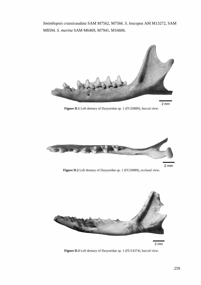
259
Sminthopsis crassicaudata SAM M7562, M7566. S. leucopus AM M13272, SAM
M8594. S. murina SAM M6469, M7941, M16606.
Figure D.1 Left dentary of Dasyuridae sp. 1 (FU20889), buccal view.
Figure D.2 Left dentary of Dasyuridae sp. 1 (FU20889), occlusal view.
Figure D.3 Left dentary of Dasyuridae sp. 1 (FU14374), buccal view.
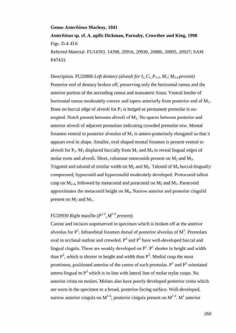
260
Genus Antechinus Macleay, 1841
Antechinus sp. cf. A. agilis Dickman, Parnaby, Crowther and King, 1998
Figs. D.4–D.6
Referred Material. FU14393. 14398, 20916, 20930, 20886, 20895, 20927; SAM
P47433.
Description. FU20886 Left dentary (alveoli for I3, C1, P1-3, M1; M2-4 present)
Posterior end of dentary broken off, preserving only the horizontal ramus and the
anterior portion of the ascending ramus and massateric fossa. Ventral border of
horizontal ramus moderately convex and tapers anteriorly from posterior end of M1.
Bone on buccal edge of alveoli for P3 is bulged as permanent premolar is un-
erupted. Notch present between alveoli of M1. No spaces between posterior and
anterior alveoli of adjacent premolars indicating crowded premolar row. Mental
foramen ventral to posterior alveolus of M1 is antero-posteriorly elongated so that it
appears oval in shape. Smaller, oval shaped mental foramen is present ventral to
alveoli for P2. M3 displaced buccally from M2 and M4 to reveal lingual edges of
molar roots and alveoli. Short, columnar entoconids present on M2 and M3.
Trigonid and talonid of similar width on M2 and M3. Talonid of M4 buccal-lingually
compressed; hypoconid and hypoconulid moderately developed. Protoconid tallest
cusp on M2-4, followed by metaconid and paraconid on M2 and M3. Paraconid
approximates the metaconid height on M4. Narrow anterior and posterior cingulid
present on M2 and M3.
FU20930 Right maxilla (P1-3, M1-4 present).
Canine and incisors unpreserved in specimen which is broken off at the anterior
alveolus for P1. Infraorbital foramen dorsal of posterior alveolus of M1. Premolars
oval in occlusal outline and crowded. P2 and P3 have well-developed buccal and
lingual cingula. These are weakly developed on P1. P1 shorter in height and width
than P2, which is shorter in height and width than P3. Medial cusp the most
prominent, positioned anterior of the centre of each premolar. P1 and P2 orientated
antero-lingual to P3 which is in-line with lateral line of molar stylar cusps. No
anterior crista on molars. Molars also have poorly developed posterior crista which
are worn in the specimen to a broad, posterior-facing surface. Well-developed,
narrow anterior cingula on M1-4; posterior cingula present on M1-3. M1 anterior
261
cingulum extends to trigon basin. Stylar cusp D broad in M1, reduced in size in M2
and smallest on M3. Metacone most prominent cusp on M1-3; paracone shorter than
stylar cusp D. Metaloph notch lingual of metaconule of M1 and M2. M4 is shaped
like a transverse bar in occlusal outline, posterior edge rounded with wear.
Remarks. Smaller overall molar size and molar row length of specimen is more
similar to A. agilis/A. stuartii than A. flavipes, A. swainsonii and A. minimus which
are generally larger overall. Presence of small, columnar entoconid on M3 contrasts
with A. flavipes which typically lacks an entoconid on M3 (Dickman et al., 1998).
Talonid of M4 in A. flavipes only made up of one cusp (reduced hypoconid),
compared with two in A. agilis, A. stuartii and A. minimus (Van Dyck, 2002).
Anterior cingulum of M1 in A. agilis/A. stuartii extends into trigon basin; terminates
at base of paraconid in A. flavipes.
Only minor maxillary, dentary and dental characters distinguish A. agilis from A.
stuartii (Dickman et al., 1998; Crowther, 2002). As a result of the poor preservation
and fragmentary nature of the fossil specimens, distinguishing the two species based
on these characters is very difficult. Differentiation is also confounded by the high
degree of morphological and size variability observed between populations of A.
agilis and A. stuartii (Crowther, 2002). However, based on the current distribution
of the two species, it is assumed that the specimens are more likely to be of A. agilis
than A. stuartii. This assumption is supported by the presence of cingulated upper
premolars of specimen FU20930, such that they appear shorter and wider than in A.
stuartii (Dickman et al., 1998; Crowther, 2002).
Comparative specimens. Antechinus agilis SAM M23166; AM M33343, AM
M33930. A. flavipes SAM M4747, M5800, M7512. A. minimus SAM M10176,
M13377, M11941, M22405. A. stuartii SAM M7500, M7501, M14143. A.
swainsonii SAM M7047, M15075.
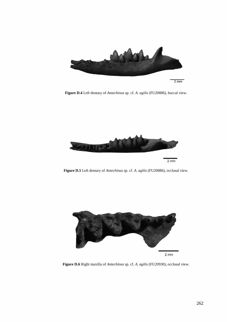
262
Figure D.4 Left dentary of Antechinus sp. cf. A. agilis (FU20886), buccal view.
Figure D.5 Left dentary of Antechinus sp. cf. A. agilis (FU20886), occlusal view.
Figure D.6 Right maxilla of Antechinus sp. cf. A. agilis (FU20930), occlusal view.
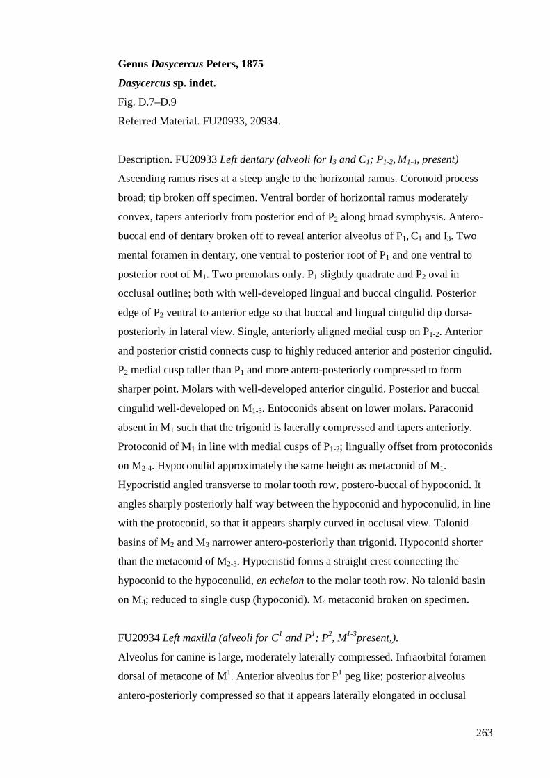
263
Genus Dasycercus Peters, 1875
Dasycercus sp. indet.
Fig. D.7–D.9
Referred Material. FU20933, 20934.
Description. FU20933 Left dentary (alveoli for I3 and C1; P1-2, M1-4, present)
Ascending ramus rises at a steep angle to the horizontal ramus. Coronoid process
broad; tip broken off specimen. Ventral border of horizontal ramus moderately
convex, tapers anteriorly from posterior end of P2 along broad symphysis. Antero-
buccal end of dentary broken off to reveal anterior alveolus of P1, C1 and I3. Two
mental foramen in dentary, one ventral to posterior root of P1 and one ventral to
posterior root of M1. Two premolars only. P1 slightly quadrate and P2 oval in
occlusal outline; both with well-developed lingual and buccal cingulid. Posterior
edge of P2 ventral to anterior edge so that buccal and lingual cingulid dip dorsa-
posteriorly in lateral view. Single, anteriorly aligned medial cusp on P1-2. Anterior
and posterior cristid connects cusp to highly reduced anterior and posterior cingulid.
P2 medial cusp taller than P1 and more antero-posteriorly compressed to form
sharper point. Molars with well-developed anterior cingulid. Posterior and buccal
cingulid well-developed on M1-3. Entoconids absent on lower molars. Paraconid
absent in M1 such that the trigonid is laterally compressed and tapers anteriorly.
Protoconid of M1 in line with medial cusps of P1-2; lingually offset from protoconids
on M2-4. Hypoconulid approximately the same height as metaconid of M1.
Hypocristid angled transverse to molar tooth row, postero-buccal of hypoconid. It
angles sharply posteriorly half way between the hypoconid and hypoconulid, in line
with the protoconid, so that it appears sharply curved in occlusal view. Talonid
basins of M2 and M3 narrower antero-posteriorly than trigonid. Hypoconid shorter
than the metaconid of M2-3. Hypocristid forms a straight crest connecting the
hypoconid to the hypoconulid, en echelon to the molar tooth row. No talonid basin
on M4; reduced to single cusp (hypoconid). M4 metaconid broken on specimen.
FU20934 Left maxilla (alveoli for C1 and P1; P2, M1-3present,).
Alveolus for canine is large, moderately laterally compressed. Infraorbital foramen
dorsal of metacone of M1. Anterior alveolus for P1 peg like; posterior alveolus
antero-posteriorly compressed so that it appears laterally elongated in occlusal
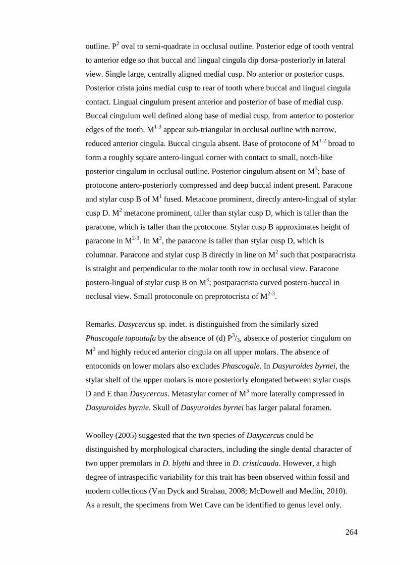
264
outline. P2 oval to semi-quadrate in occlusal outline. Posterior edge of tooth ventral
to anterior edge so that buccal and lingual cingula dip dorsa-posteriorly in lateral
view. Single large, centrally aligned medial cusp. No anterior or posterior cusps.
Posterior crista joins medial cusp to rear of tooth where buccal and lingual cingula
contact. Lingual cingulum present anterior and posterior of base of medial cusp.
Buccal cingulum well defined along base of medial cusp, from anterior to posterior
edges of the tooth. M1-3 appear sub-triangular in occlusal outline with narrow,
reduced anterior cingula. Buccal cingula absent. Base of protocone of M1-2 broad to
form a roughly square antero-lingual corner with contact to small, notch-like
posterior cingulum in occlusal outline. Posterior cingulum absent on M3; base of
protocone antero-posteriorly compressed and deep buccal indent present. Paracone
and stylar cusp B of M1 fused. Metacone prominent, directly antero-lingual of stylar
cusp D. M2 metacone prominent, taller than stylar cusp D, which is taller than the
paracone, which is taller than the protocone. Stylar cusp B approximates height of
paracone in M2-3. In M3, the paracone is taller than stylar cusp D, which is
columnar. Paracone and stylar cusp B directly in line on M2 such that postparacrista
is straight and perpendicular to the molar tooth row in occlusal view. Paracone
postero-lingual of stylar cusp B on M3; postparacrista curved postero-buccal in
occlusal view. Small protoconule on preprotocrista of M2-3.
Remarks. Dasycercus sp. indet. is distinguished from the similarly sized
Phascogale tapoatafa by the absence of (d) P3/3, absence of posterior cingulum on
M3 and highly reduced anterior cingula on all upper molars. The absence of
entoconids on lower molars also excludes Phascogale. In Dasyuroides byrnei, the
stylar shelf of the upper molars is more posteriorly elongated between stylar cusps
D and E than Dasycercus. Metastylar corner of M3 more laterally compressed in
Dasyuroides byrnie. Skull of Dasyuroides byrnei has larger palatal foramen.
Woolley (2005) suggested that the two species of Dasycercus could be
distinguished by morphological characters, including the single dental character of
two upper premolars in D. blythi and three in D. cristicauda. However, a high
degree of intraspecific variability for this trait has been observed within fossil and
modern collections (Van Dyck and Strahan, 2008; McDowell and Medlin, 2010).
As a result, the specimens from Wet Cave can be identified to genus level only.
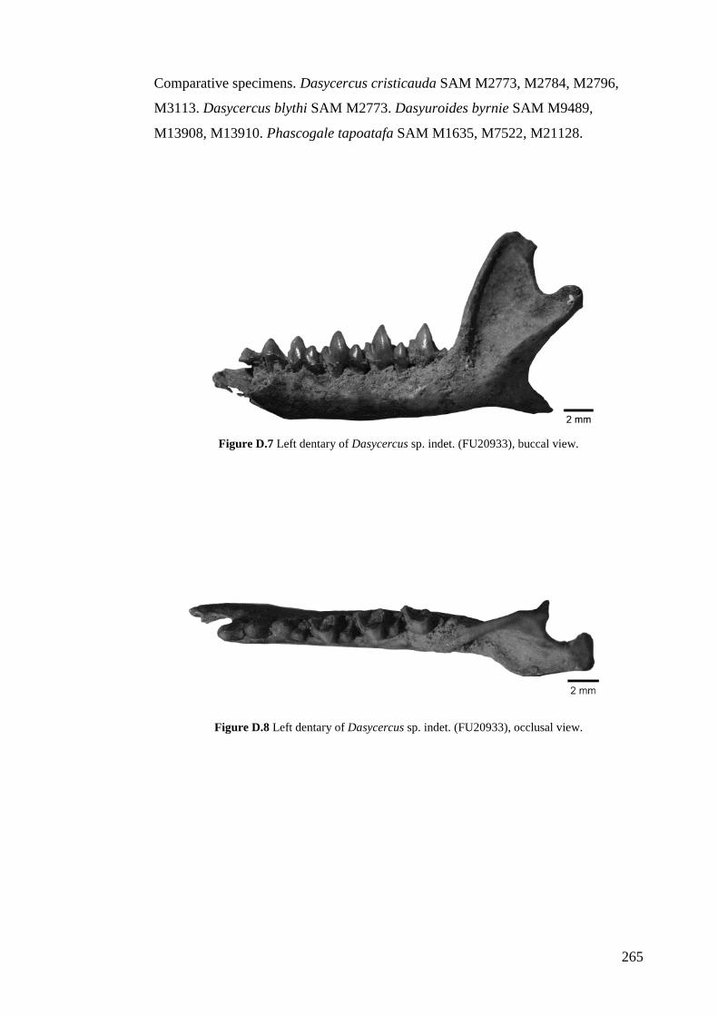
265
Comparative specimens. Dasycercus cristicauda SAM M2773, M2784, M2796,
M3113. Dasycercus blythi SAM M2773. Dasyuroides byrnie SAM M9489,
M13908, M13910. Phascogale tapoatafa SAM M1635, M7522, M21128.
Figure D.7 Left dentary of Dasycercus sp. indet. (FU20933), buccal view.
Figure D.8 Left dentary of Dasycercus sp. indet. (FU20933), occlusal view.
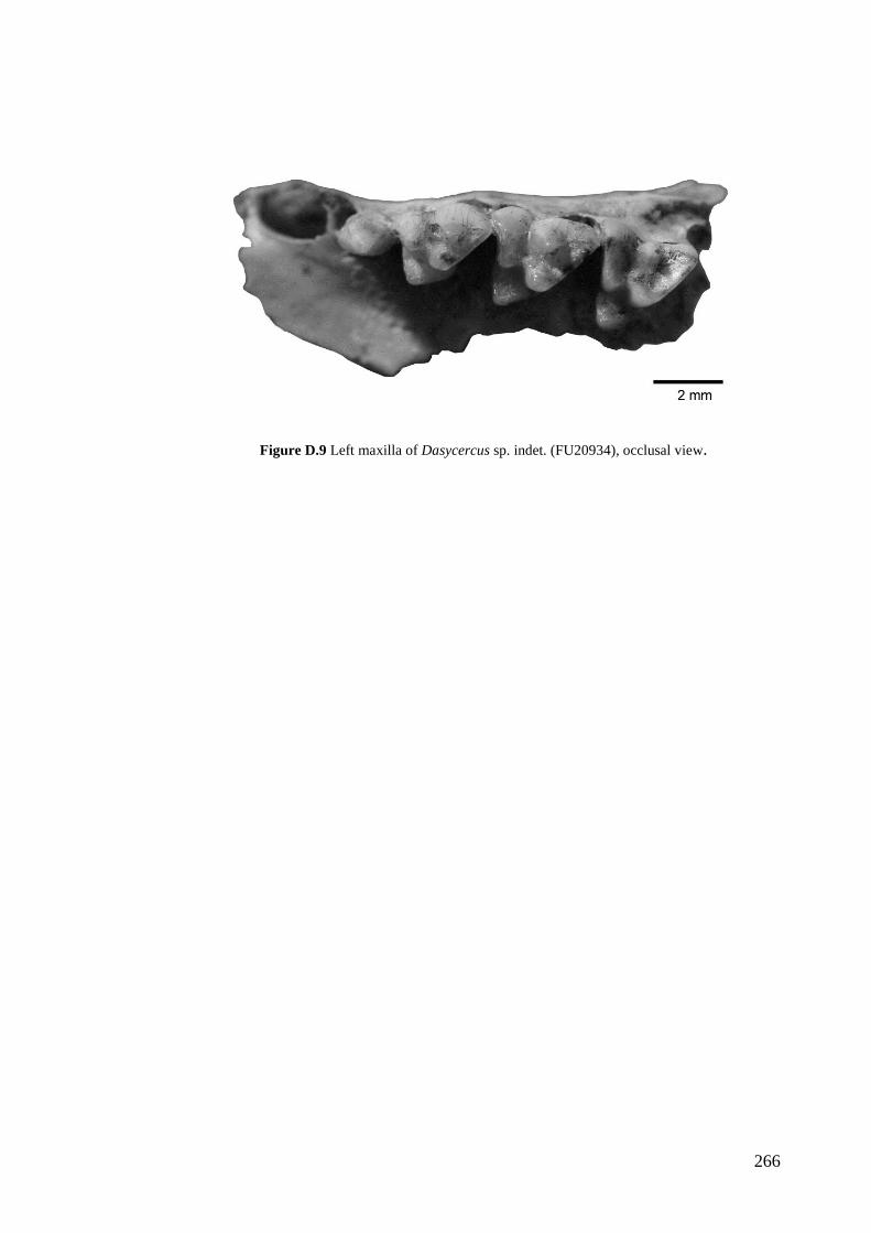
266
Figure D.9 Left maxilla of Dasycercus sp. indet. (FU20934), occlusal view.
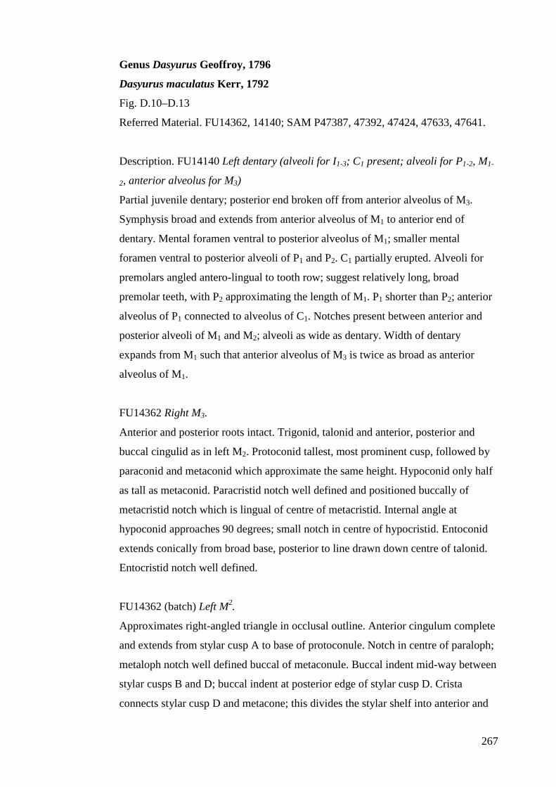
267
Genus Dasyurus Geoffroy, 1796
Dasyurus maculatus Kerr, 1792
Fig. D.10–D.13
Referred Material. FU14362, 14140; SAM P47387, 47392, 47424, 47633, 47641.
Description. FU14140 Left dentary (alveoli for I1-3; C1 present; alveoli for P1-2, M1-
2, anterior alveolus for M3)
Partial juvenile dentary; posterior end broken off from anterior alveolus of M3.
Symphysis broad and extends from anterior alveolus of M1 to anterior end of
dentary. Mental foramen ventral to posterior alveolus of M1; smaller mental
foramen ventral to posterior alveoli of P1 and P2. C1 partially erupted. Alveoli for
premolars angled antero-lingual to tooth row; suggest relatively long, broad
premolar teeth, with P2 approximating the length of M1. P1 shorter than P2; anterior
alveolus of P1 connected to alveolus of C1. Notches present between anterior and
posterior alveoli of M1 and M2; alveoli as wide as dentary. Width of dentary
expands from M1 such that anterior alveolus of M3 is twice as broad as anterior
alveolus of M1.
FU14362 Right M3.
Anterior and posterior roots intact. Trigonid, talonid and anterior, posterior and
buccal cingulid as in left M2. Protoconid tallest, most prominent cusp, followed by
paraconid and metaconid which approximate the same height. Hypoconid only half
as tall as metaconid. Paracristid notch well defined and positioned buccally of
metacristid notch which is lingual of centre of metacristid. Internal angle at
hypoconid approaches 90 degrees; small notch in centre of hypocristid. Entoconid
extends conically from broad base, posterior to line drawn down centre of talonid.
Entocristid notch well defined.
FU14362 (batch) Left M2.
Approximates right-angled triangle in occlusal outline. Anterior cingulum complete
and extends from stylar cusp A to base of protoconule. Notch in centre of paraloph;
metaloph notch well defined buccal of metaconule. Buccal indent mid-way between
stylar cusps B and D; buccal indent at posterior edge of stylar cusp D. Crista
connects stylar cusp D and metacone; this divides the stylar shelf into anterior and
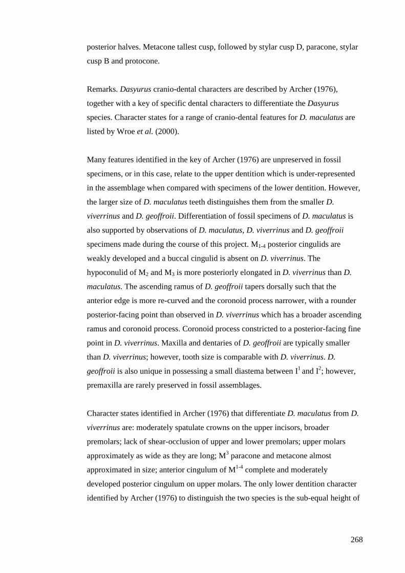
268
posterior halves. Metacone tallest cusp, followed by stylar cusp D, paracone, stylar
cusp B and protocone.
Remarks. Dasyurus cranio-dental characters are described by Archer (1976),
together with a key of specific dental characters to differentiate the Dasyurus
species. Character states for a range of cranio-dental features for D. maculatus are
listed by Wroe et al. (2000).
Many features identified in the key of Archer (1976) are unpreserved in fossil
specimens, or in this case, relate to the upper dentition which is under-represented
in the assemblage when compared with specimens of the lower dentition. However,
the larger size of D. maculatus teeth distinguishes them from the smaller D.
viverrinus and D. geoffroii. Differentiation of fossil specimens of D. maculatus is
also supported by observations of D. maculatus, D. viverrinus and D. geoffroii
specimens made during the course of this project. M1-4 posterior cingulids are
weakly developed and a buccal cingulid is absent on D. viverrinus. The
hypoconulid of M2 and M3 is more posteriorly elongated in D. viverrinus than D.
maculatus. The ascending ramus of D. geoffroii tapers dorsally such that the
anterior edge is more re-curved and the coronoid process narrower, with a rounder
posterior-facing point than observed in D. viverrinus which has a broader ascending
ramus and coronoid process. Coronoid process constricted to a posterior-facing fine
point in D. viverrinus. Maxilla and dentaries of D. geoffroii are typically smaller
than D. viverrinus; however, tooth size is comparable with D. viverrinus. D.
geoffroii is also unique in possessing a small diastema between I1 and I2; however,
premaxilla are rarely preserved in fossil assemblages.
Character states identified in Archer (1976) that differentiate D. maculatus from D.
viverrinus are: moderately spatulate crowns on the upper incisors, broader
premolars; lack of shear-occlusion of upper and lower premolars; upper molars
approximately as wide as they are long; M3 paracone and metacone almost
approximated in size; anterior cingulum of M1-4 complete and moderately
developed posterior cingulum on upper molars. The only lower dentition character
identified by Archer (1976) to distinguish the two species is the sub-equal height of
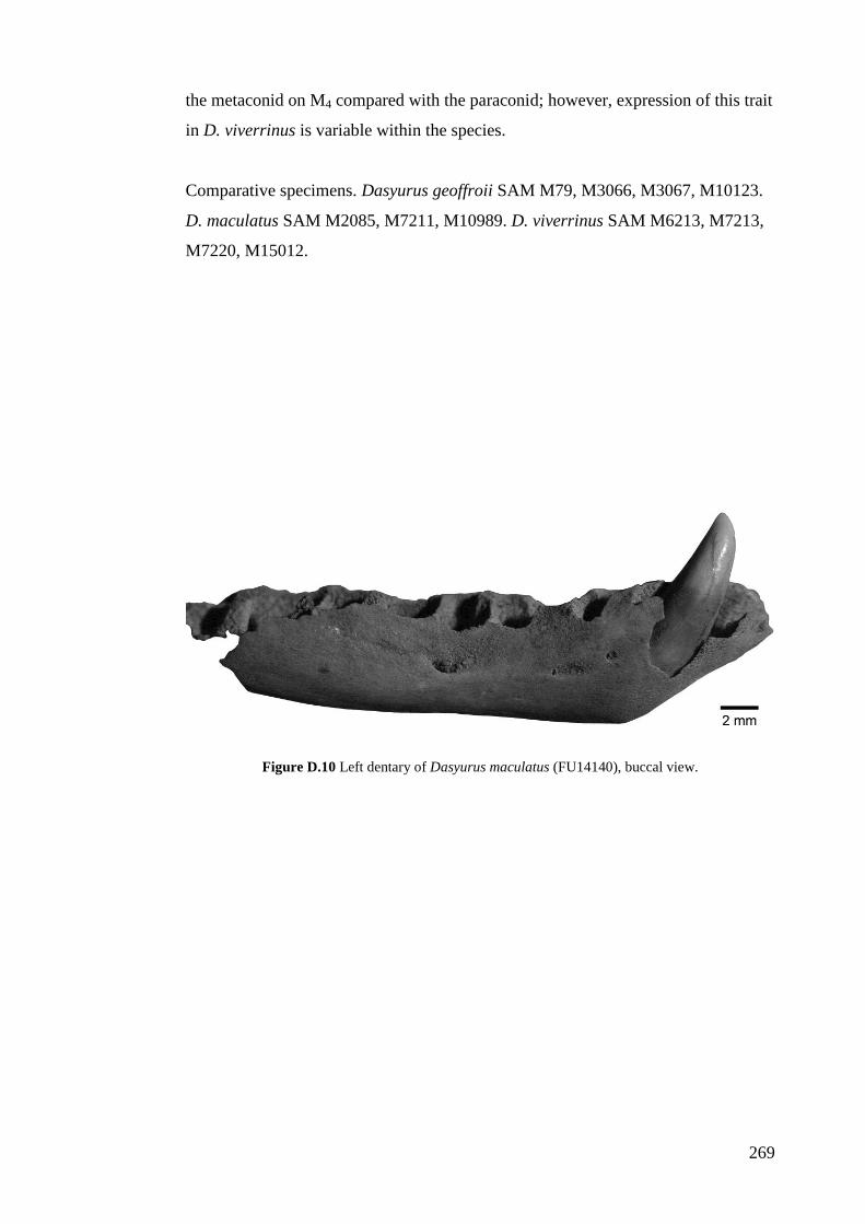
269
the metaconid on M4 compared with the paraconid; however, expression of this trait
in D. viverrinus is variable within the species.
Comparative specimens. Dasyurus geoffroii SAM M79, M3066, M3067, M10123.
D. maculatus SAM M2085, M7211, M10989. D. viverrinus SAM M6213, M7213,
M7220, M15012.
Figure D.10 Left dentary of Dasyurus maculatus (FU14140), buccal view.
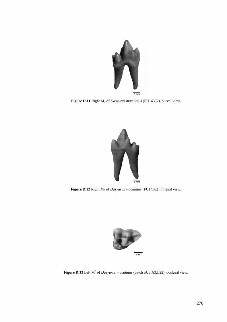
270
Figure D.11 Right M3 of Dasyurus maculatus (FU14362), buccal view.
Figure D.12 Right M3 of Dasyurus maculatus (FU14362), lingual view.
Figure D.13 Left M2 of Dasyurus maculatus (batch 5U6 A3:L22), occlusal view.
271
Genus Phascogale Temminck, 1824
Phascogale calura Gould, 1844
Fig. D.14–D.16
Referred Material. FU20641, 20645, 20657; SAM P47432.
Description. SAM P47432 Left maxilla (alveolus for C1; P1-3, M1-4present). Gen. et
sp. cf. Phascogale calura.
Anterior portion of maxilla complete with suture to premaxilla visible as a narrow
groove. Infraorbital foramen dorsal of anterior half of M1. Alveolus for C1 large,
broader than premolars and length approximates combined length of P1-2. P1-3 with
well-developed buccal and lingual cingula. Posterior end of P1 rounded in occlusal
outline, tapers to antero-buccally inclined tip. P2 oval in occlusal outline with slight
lateral compression at the middle of the buccal and lingual sides. Anterior end of P3
broader than posterior end in occlusal outline. Medial cusps of P1-3 tall, weighted
over anterior portion of each respective tooth. Posterior crista connects tip of medial
cusp with small posterior cusp of P1-3.
M1 stylar cusp A contacts buccal side of posterior cusp of P3. Well-developed
anterior cingula on M1-4. Posterior cingula present on M1-4; extends postero-
buccally on M1-3 to form a very thin ledge of enamel ventral of metacone and which
extends to half-way along the length of the metacrista. Stylar cusp B and paracone
of M1 are separated by a short paracrista. M1-2 metacone approximates the height
and size of stylar cusp D. Metacone of M3 is slightly taller and broader than stylar
cusp D. Stylar cusp B and the paracone approximate the same height on M1-2.
Anterior border of M2-4 approximately 90 degrees to buccal border of molar tooth
row. Inside angle of M2-3 protocone antero-posteriorly compressed so that molars
are triangular in occlusal view but not equilateral; trigon basin circular in occlusal
outline. M2-3 postparacrista v-shaped as lingual angle between paracone and
metacone is acute. M4 paracone largest cusp; transverse bar in occlusal outline with
short posterior projection of the highly reduced metacone.
FU20645 Left Dentary (alveoli for M2-4)
Anterior end of dentary broken off from M2. Ascending ramus broken off at just
above the level of the tooth row. Ventral border of horizontal ramus convex. Mental
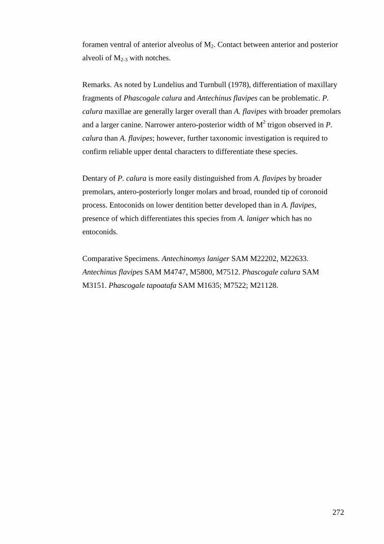
272
foramen ventral of anterior alveolus of M2. Contact between anterior and posterior
alveoli of M2-3 with notches.
Remarks. As noted by Lundelius and Turnbull (1978), differentiation of maxillary
fragments of Phascogale calura and Antechinus flavipes can be problematic. P.
calura maxillae are generally larger overall than A. flavipes with broader premolars
and a larger canine. Narrower antero-posterior width of M2 trigon observed in P.
calura than A. flavipes; however, further taxonomic investigation is required to
confirm reliable upper dental characters to differentiate these species.
Dentary of P. calura is more easily distinguished from A. flavipes by broader
premolars, antero-posteriorly longer molars and broad, rounded tip of coronoid
process. Entoconids on lower dentition better developed than in A. flavipes,
presence of which differentiates this species from A. laniger which has no
entoconids.
Comparative Specimens. Antechinomys laniger SAM M22202, M22633.
Antechinus flavipes SAM M4747, M5800, M7512. Phascogale calura SAM
M3151. Phascogale tapoatafa SAM M1635; M7522; M21128.
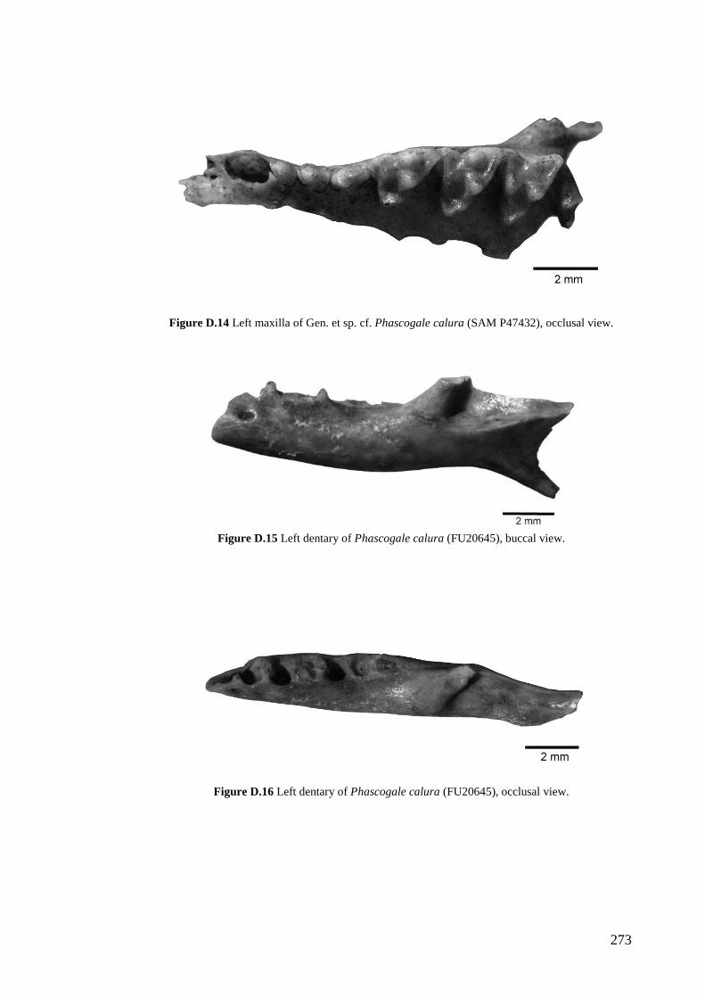
273
Figure D.14 Left maxilla of Gen. et sp. cf. Phascogale calura (SAM P47432), occlusal view.
Figure D.15 Left dentary of Phascogale calura (FU20645), buccal view.
Figure D.16 Left dentary of Phascogale calura (FU20645), occlusal view.
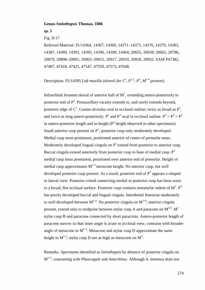
274
Genus Sminthopsis Thomas, 1886
sp. 1
Fig. D.17
Referred Material. FU14364, 14367, 14369, 14371–14373, 14376, 14379, 14383,
14387, 14389, 14391, 14395, 14396, 14399, 14404, 20655, 20658, 20665, 20786,
20879, 20898–20901, 20903–20915, 20917, 20919, 20928, 20932. SAM P47382,
47407, 47418, 47425, 47547, 47559, 47573, 47648.
Description. FU14395 Left maxilla (alveoli for C1, P1,2; P3, M1-4 present).
Infraorbital foramen dorsal of anterior half of M1, extending antero-posteriorly to
posterior end of P3. Premaxillary vacuity extends to, and rarely extends beyond,
posterior edge of C1. Canine alveolus oval in occlusal outline; twice as broad as P1,
and twice as long antero-posteriorly. P1 and P3 oval in occlusal outline. P3 > P2 > P1
in antero-posterior length and in height (P2 height observed in other specimens).
Small anterior cusp present on P1; posterior cusp only moderately developed.
Medial cusp most prominent, positioned anterior of centre of premolar mass.
Moderately developed lingual cingula on P1 extend from posterior to anterior cusp.
Buccal cingula extend anteriorly from posterior cusp to base of medial cusp. P3
medial cusp most prominent, positioned over anterior end of premolar. Height of
medial cusp approximates M1-3 metacone height. No anterior cusp, but well
developed posterior cusp present. As a result, posterior end of P3 appears v-shaped
in lateral view. Posterior cristid connecting medial to posterior cusp has been worn
to a broad, flat occlusal surface. Posterior cusp contacts metastylar indent of M1. P3
has poorly developed buccal and lingual cingula. Interdental fenestrae moderately
to well developed between M1-4. No posterior cingula on M1-4; anterior cingula
present, extend only to midpoint between stylar cusp A and paracone on M3,4. M1
stylar cusp B and paracone connected by short paracrista. Antero-posterior length of
paracone narrow so that inner angle is acute in occlusal view, contrasts with broader
angle of metacone in M1-3. Metacone and stylar cusp D approximate the same
height in M1,2; stylar cusp D not as high as metacone on M3.
Remarks. Specimens identified as Sminthopsis by absence of posterior cingula on
M1-3, contrasting with Phascogale and Antechinus. Although A. minimus does not
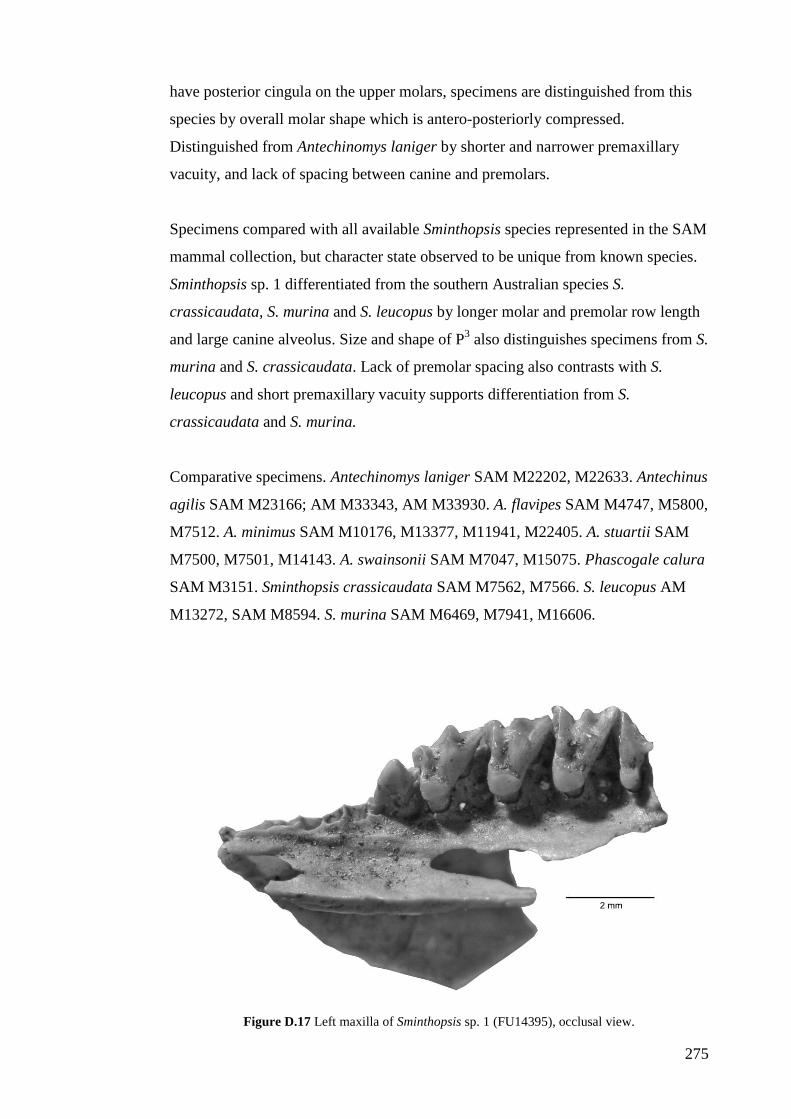
275
have posterior cingula on the upper molars, specimens are distinguished from this
species by overall molar shape which is antero-posteriorly compressed.
Distinguished from Antechinomys laniger by shorter and narrower premaxillary
vacuity, and lack of spacing between canine and premolars.
Specimens compared with all available Sminthopsis species represented in the SAM
mammal collection, but character state observed to be unique from known species.
Sminthopsis sp. 1 differentiated from the southern Australian species S.
crassicaudata, S. murina and S. leucopus by longer molar and premolar row length
and large canine alveolus. Size and shape of P3 also distinguishes specimens from S.
murina and S. crassicaudata. Lack of premolar spacing also contrasts with S.
leucopus and short premaxillary vacuity supports differentiation from S.
crassicaudata and S. murina.
Comparative specimens. Antechinomys laniger SAM M22202, M22633. Antechinus
agilis SAM M23166; AM M33343, AM M33930. A. flavipes SAM M4747, M5800,
M7512. A. minimus SAM M10176, M13377, M11941, M22405. A. stuartii SAM
M7500, M7501, M14143. A. swainsonii SAM M7047, M15075. Phascogale calura
SAM M3151. Sminthopsis crassicaudata SAM M7562, M7566. S. leucopus AM
M13272, SAM M8594. S. murina SAM M6469, M7941, M16606.
Figure D.17 Left maxilla of Sminthopsis sp. 1 (FU14395), occlusal view.
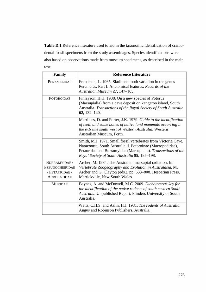
276
Table D.1 Reference literature used to aid in the taxonomic identification of cranio-
dental fossil specimens from the study assemblages. Species identifications were
also based on observations made from museum specimens, as described in the main
text.
Family Reference Literature
PERAMELIDAE Freedman, L. 1965. Skull and tooth variation in the genus Perameles. Part I: Anatomical features. Records of the Australian Museum 27, 147–165.
POTOROIDAE Finlayson, H.H. 1938. On a new species of Potorus (Marsupialia) from a cave deposit on kangaroo island, South Australia. Transactions of the Royal Society of South Australia 62, 132–140.
Merrilees, D. and Porter, J.K. 1979. Guide to the identification of teeth and some bones of native land mammals occurring in the extreme south west of Western Australia. Western Australian Museum, Perth.
Smith, M.J. 1971. Small fossil vertebrates from Victoria Cave, Naracoorte, South Australia. I. Potoroinae (Macropodidae), Petauridae and Burramyidae (Marsupialia). Transactions of the Royal Society of South Australia 95, 185–198.
BURRAMYIDAE / PSEUDOCHEIRIDAE
/ PETAURIDAE / ACROBATIDAE
Archer, M. 1984. The Australian marsupial radiation. In: Vertebrate Zoogeography and Evolution in Australasia. M. Archer and G. Clayton (eds.), pp. 633–808. Hesperian Press, Merrickville, New South Wales.
MURIDAE Baynes, A. and McDowell, M.C. 2009. Dichotomous key for the identification of the native rodents of south eastern South Australia. Unpublished Report. Flinders University of South Australia.
Watts, C.H.S. and Aslin, H.J. 1981. The rodents of Australia. Angus and Robinson Publishers, Australia.
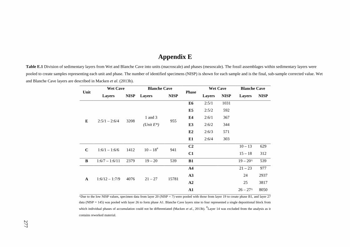
277
Appendix E Table E.1 Division of sedimentary layers from Wet and Blanche Cave into units (macroscale) and phases (mesoscale). The fossil assemblages within sedimentary layers were
pooled to create samples representing each unit and phase. The number of identified specimens (NISP) is shown for each sample and is the final, sub-sample corrected value. Wet
and Blanche Cave layers are described in Macken et al. (2013b).
Unit Wet Cave Blanche Cave
Phase Wet Cave Blanche Cave
Layers NISP Layers NISP Layers NISP Layers NISP
E 2:5/1 – 2:6/4 3208 1 and 3
(Unit E*) 955
E6 2:5/1 1031
E5 2:5/2 592
E4 2:6/1 367
E3 2:6/2 344
E2 2:6/3 571
E1 2:6/4 303
C 1:6/1 – 1:6/6 1412 10 – 18# 941 C2 10 – 13 629
C1 15 – 18 312
B 1:6/7 – 1:6/11 2379 19 – 20 539 B1 19 – 20^ 539
A 1:6/12 – 1:7/9 4076 21 – 27 15781
A4 21 – 23 977
A3 24 2937
A2 25 3817
A1 26 – 27^ 8050 ^Due to the low NISP values, specimen data from layer 20 (NISP = 7) were pooled with those from layer 19 to create phase B1, and layer 27
data (NISP = 145) was pooled with layer 26 to form phase A1. Blanche Cave layers nine to four represented a single depositional block from
which individual phases of accumulation could not be differentiated (Macken et al., 2013b). #Layer 14 was excluded from the analysis as it
contains reworked material.
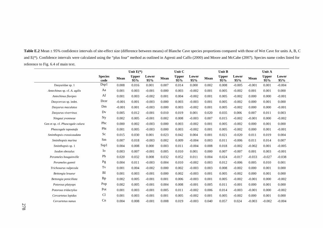
278
Table E.2 Mean ± 95% confidence intervals of site-effect size (difference between means) of Blanche Cave species proportions compared with those of Wet Cave for units A, B, C
and E(*). Confidence intervals were calculated using the “plus four” method as outlined in Agresti and Caffo (2000) and Moore and McCabe (2007). Species name codes listed for
reference to Fig. 6.4 of main text.
Unit E(*) Unit C Unit B Unit A
Species code Mean Upper
95% Lower 95% Mean Upper
95% Lower 95% Mean Upper
95% Lower 95% Mean Upper
95% Lower 95%
Dasyuridae sp. 1 Dsp1 0.008 0.016 0.001 0.007 0.014 0.000 0.002 0.008 -0.005 -0.001 0.001 -0.004 Antechinus sp. cf. A. agilis Aa 0.001 0.003 -0.001 0.000 0.003 -0.002 0.001 0.005 -0.002 0.001 0.001 0.000
Antechinus flavipes Af 0.001 0.003 -0.002 0.001 0.004 -0.002 0.001 0.005 -0.002 0.000 0.000 -0.001 Dasycercus sp. indet. Dcer -0.001 0.001 -0.003 0.000 0.003 -0.003 0.001 0.005 -0.002 0.000 0.001 0.000 Dasyurus maculatus Dm -0.001 0.001 -0.003 0.000 0.003 -0.002 0.001 0.005 -0.002 0.000 0.000 -0.001 Dasyurus viverrinus Dv 0.005 0.012 -0.001 0.010 0.019 0.001 0.020 0.035 0.006 0.007 0.011 0.003 Ningaui yvonneae Ny 0.002 0.005 -0.001 0.002 0.008 -0.003 0.007 0.015 -0.002 -0.001 0.000 -0.002
Gen et sp. cf. Phascogale calura Phc 0.000 0.002 -0.003 0.000 0.003 -0.002 0.001 0.005 -0.002 0.000 0.001 0.000 Phascogale tapoatafa Pht 0.001 0.005 -0.003 0.000 0.003 -0.002 0.001 0.005 -0.002 0.000 0.001 -0.001
Sminthopsis crassicaudata Sc 0.015 0.030 0.001 0.023 0.042 0.004 0.001 0.021 -0.020 0.011 0.019 0.004 Sminthopsis murina Sm 0.007 0.018 -0.003 0.002 0.009 -0.004 0.003 0.011 -0.006 0.011 0.014 0.007 Sminthopsis sp. 1 Ssp1 0.004 0.008 0.000 0.003 0.011 -0.004 0.008 0.018 -0.002 -0.002 0.001 -0.005 Isodon obesulus Io 0.003 0.007 -0.001 0.005 0.010 0.001 0.000 0.007 -0.007 0.001 0.003 -0.001
Perameles bougainville Pb 0.020 0.032 0.008 0.032 0.052 0.011 0.004 0.024 -0.017 -0.033 -0.027 -0.038 Perameles gunnii Pg 0.004 0.011 -0.003 0.004 0.010 -0.002 0.003 0.012 -0.006 0.005 0.010 0.001
Trichosurus vulpecula Tv 0.001 0.004 -0.002 0.000 0.002 -0.003 0.003 0.008 -0.002 0.000 0.001 0.000 Bettongia lesueur Bl 0.001 0.003 -0.001 0.000 0.002 -0.003 0.001 0.005 -0.002 0.000 0.001 0.000
Bettongia penicillata Bp 0.002 0.005 -0.001 0.001 0.006 -0.003 0.001 0.005 -0.002 -0.001 0.000 -0.002 Potorous platyops Pop 0.002 0.005 -0.001 0.004 0.008 -0.001 0.005 0.011 -0.001 0.000 0.001 0.000
Potorous tridactylus Pot 0.001 0.003 -0.001 0.005 0.011 -0.002 0.006 0.014 -0.003 -0.001 0.000 -0.002 Cercartetus lepidus Cl 0.001 0.003 -0.001 0.001 0.005 -0.002 0.001 0.005 -0.002 0.000 0.001 0.000 Cercartetus nanus Cn 0.004 0.008 -0.001 0.008 0.019 -0.003 0.040 0.057 0.024 -0.003 -0.002 -0.004
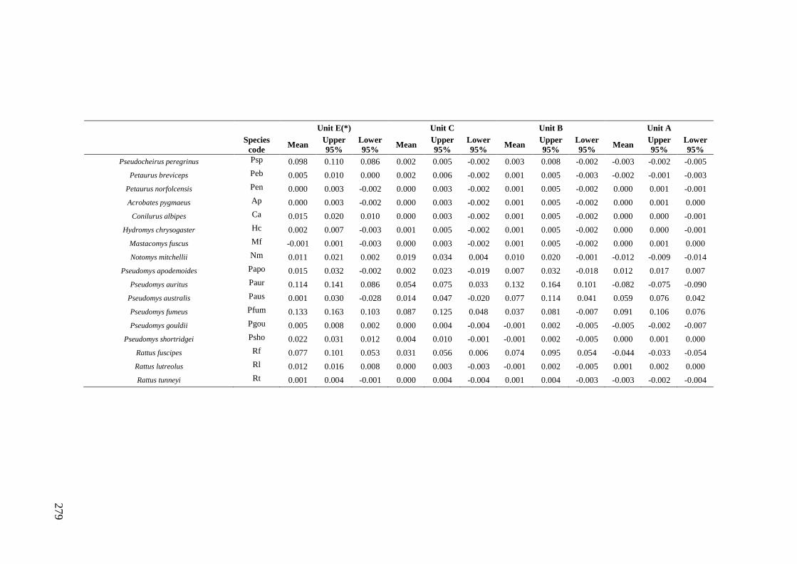
279
Unit E(*) Unit C Unit B Unit A
Species code Mean Upper
95% Lower 95% Mean Upper
95% Lower 95% Mean Upper
95% Lower 95% Mean Upper
95% Lower 95%
Pseudocheirus peregrinus Psp 0.098 0.110 0.086 0.002 0.005 -0.002 0.003 0.008 -0.002 -0.003 -0.002 -0.005 Petaurus breviceps Peb 0.005 0.010 0.000 0.002 0.006 -0.002 0.001 0.005 -0.003 -0.002 -0.001 -0.003
Petaurus norfolcensis Pen 0.000 0.003 -0.002 0.000 0.003 -0.002 0.001 0.005 -0.002 0.000 0.001 -0.001 Acrobates pygmaeus Ap 0.000 0.003 -0.002 0.000 0.003 -0.002 0.001 0.005 -0.002 0.000 0.001 0.000
Conilurus albipes Ca 0.015 0.020 0.010 0.000 0.003 -0.002 0.001 0.005 -0.002 0.000 0.000 -0.001 Hydromys chrysogaster Hc 0.002 0.007 -0.003 0.001 0.005 -0.002 0.001 0.005 -0.002 0.000 0.000 -0.001
Mastacomys fuscus Mf -0.001 0.001 -0.003 0.000 0.003 -0.002 0.001 0.005 -0.002 0.000 0.001 0.000 Notomys mitchellii Nm 0.011 0.021 0.002 0.019 0.034 0.004 0.010 0.020 -0.001 -0.012 -0.009 -0.014
Pseudomys apodemoides Papo 0.015 0.032 -0.002 0.002 0.023 -0.019 0.007 0.032 -0.018 0.012 0.017 0.007 Pseudomys auritus Paur 0.114 0.141 0.086 0.054 0.075 0.033 0.132 0.164 0.101 -0.082 -0.075 -0.090
Pseudomys australis Paus 0.001 0.030 -0.028 0.014 0.047 -0.020 0.077 0.114 0.041 0.059 0.076 0.042 Pseudomys fumeus Pfum 0.133 0.163 0.103 0.087 0.125 0.048 0.037 0.081 -0.007 0.091 0.106 0.076 Pseudomys gouldii Pgou 0.005 0.008 0.002 0.000 0.004 -0.004 -0.001 0.002 -0.005 -0.005 -0.002 -0.007
Pseudomys shortridgei Psho 0.022 0.031 0.012 0.004 0.010 -0.001 -0.001 0.002 -0.005 0.000 0.001 0.000 Rattus fuscipes Rf 0.077 0.101 0.053 0.031 0.056 0.006 0.074 0.095 0.054 -0.044 -0.033 -0.054 Rattus lutreolus Rl 0.012 0.016 0.008 0.000 0.003 -0.003 -0.001 0.002 -0.005 0.001 0.002 0.000 Rattus tunneyi Rt 0.001 0.004 -0.001 0.000 0.004 -0.004 0.001 0.004 -0.003 -0.003 -0.002 -0.004
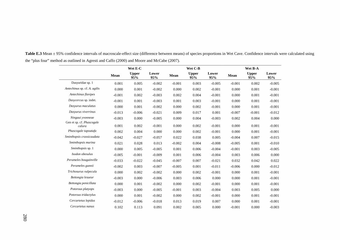
280
Table E.3 Mean ± 95% confidence intervals of macroscale-effect size (difference between means) of species proportions in Wet Cave. Confidence intervals were calculated using
the “plus four” method as outlined in Agresti and Caffo (2000) and Moore and McCabe (2007).
Wet E-C Wet C-B Wet B-A
Mean Upper 95%
Lower 95% Mean Upper
95% Lower 95% Mean Upper
95% Lower 95%
Dasyuridae sp. 1 0.001 0.005 -0.002 -0.001 0.003 -0.005 -0.001 0.002 -0.005 Antechinus sp. cf. A. agilis 0.000 0.001 -0.002 0.000 0.002 -0.001 0.000 0.001 -0.001
Antechinus flavipes -0.001 0.002 -0.003 0.002 0.004 -0.001 0.000 0.001 -0.001 Dasycercus sp. indet. -0.001 0.001 -0.003 0.001 0.003 -0.001 0.000 0.001 -0.001 Dasyurus maculatus 0.000 0.001 -0.002 0.000 0.002 -0.001 0.000 0.001 -0.001 Dasyurus viverrinus -0.013 -0.006 -0.021 0.009 0.017 0.001 -0.007 -0.001 -0.012 Ningaui yvonneae -0.003 0.000 -0.005 0.000 0.004 -0.003 0.002 0.004 0.000
Gen et sp. cf. Phascogale calura 0.001 0.002 -0.001 0.000 0.002 -0.001 0.000 0.001 -0.001
Phascogale tapoatafa 0.002 0.004 0.000 0.000 0.002 -0.001 0.000 0.001 -0.001 Sminthopsis crassicaudata -0.042 -0.027 -0.057 0.022 0.038 0.005 -0.004 0.007 -0.015
Sminthopsis murina 0.021 0.028 0.013 -0.002 0.004 -0.008 -0.005 0.001 -0.010 Sminthopsis sp. 1 0.000 0.005 -0.005 0.001 0.006 -0.004 -0.001 0.003 -0.005 Isodon obesulus -0.005 -0.001 -0.009 0.001 0.006 -0.004 0.003 0.006 0.000
Perameles bougainville -0.033 -0.022 -0.045 -0.007 0.007 -0.021 0.032 0.042 0.022 Perameles gunnii -0.002 0.003 -0.007 -0.005 0.001 -0.011 -0.006 0.000 -0.012
Trichosurus vulpecula 0.000 0.002 -0.002 0.000 0.002 -0.001 0.000 0.001 -0.001 Bettongia lesueur -0.003 0.000 -0.006 0.003 0.006 0.000 0.000 0.001 -0.001
Bettongia penicillata 0.000 0.001 -0.002 0.000 0.002 -0.001 0.000 0.001 -0.001 Potorous platyops -0.003 0.000 -0.005 -0.001 0.003 -0.004 0.003 0.005 0.000
Potorous tridactylus 0.000 0.001 -0.002 0.000 0.002 -0.001 0.000 0.001 -0.001 Cercartetus lepidus -0.012 -0.006 -0.018 0.013 0.019 0.007 0.000 0.001 -0.001 Cercartetus nanus 0.102 0.113 0.091 0.002 0.005 0.000 -0.001 0.000 -0.003
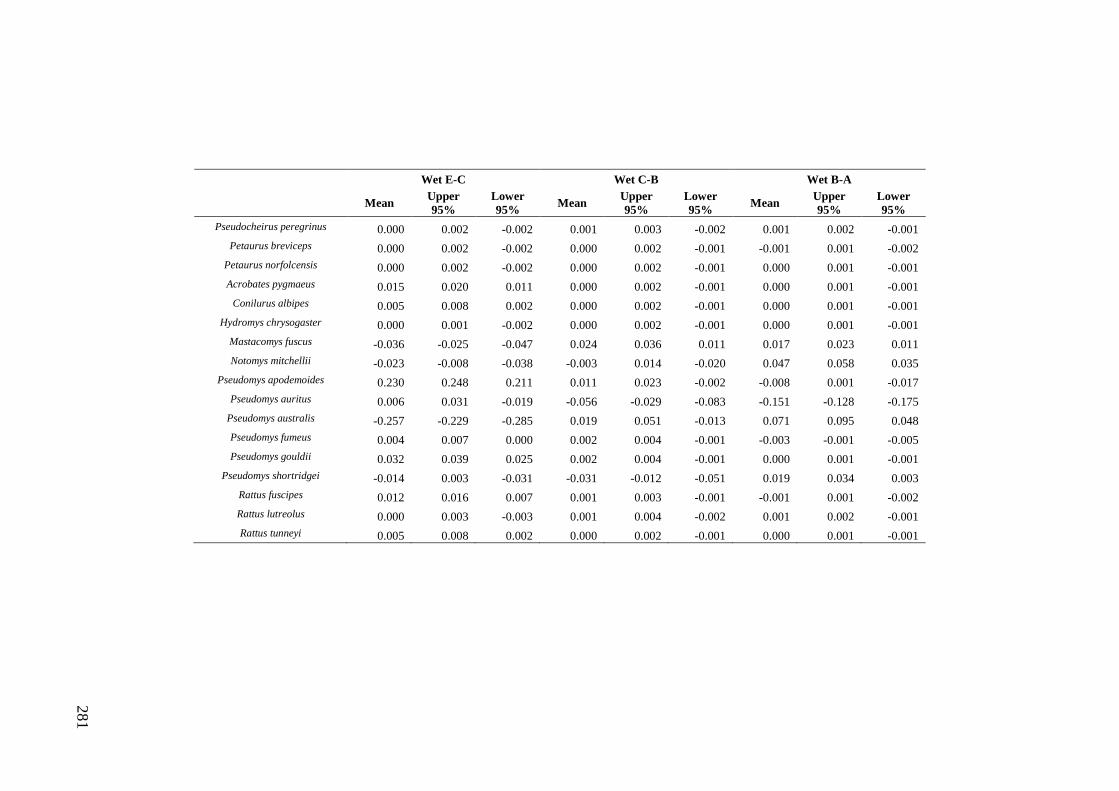
281
Wet E-C Wet C-B Wet B-A
Mean Upper 95%
Lower 95% Mean Upper
95% Lower 95% Mean Upper
95% Lower 95%
Pseudocheirus peregrinus 0.000 0.002 -0.002 0.001 0.003 -0.002 0.001 0.002 -0.001 Petaurus breviceps 0.000 0.002 -0.002 0.000 0.002 -0.001 -0.001 0.001 -0.002
Petaurus norfolcensis 0.000 0.002 -0.002 0.000 0.002 -0.001 0.000 0.001 -0.001 Acrobates pygmaeus 0.015 0.020 0.011 0.000 0.002 -0.001 0.000 0.001 -0.001
Conilurus albipes 0.005 0.008 0.002 0.000 0.002 -0.001 0.000 0.001 -0.001 Hydromys chrysogaster 0.000 0.001 -0.002 0.000 0.002 -0.001 0.000 0.001 -0.001
Mastacomys fuscus -0.036 -0.025 -0.047 0.024 0.036 0.011 0.017 0.023 0.011 Notomys mitchellii -0.023 -0.008 -0.038 -0.003 0.014 -0.020 0.047 0.058 0.035
Pseudomys apodemoides 0.230 0.248 0.211 0.011 0.023 -0.002 -0.008 0.001 -0.017 Pseudomys auritus 0.006 0.031 -0.019 -0.056 -0.029 -0.083 -0.151 -0.128 -0.175
Pseudomys australis -0.257 -0.229 -0.285 0.019 0.051 -0.013 0.071 0.095 0.048 Pseudomys fumeus 0.004 0.007 0.000 0.002 0.004 -0.001 -0.003 -0.001 -0.005 Pseudomys gouldii 0.032 0.039 0.025 0.002 0.004 -0.001 0.000 0.001 -0.001
Pseudomys shortridgei -0.014 0.003 -0.031 -0.031 -0.012 -0.051 0.019 0.034 0.003 Rattus fuscipes 0.012 0.016 0.007 0.001 0.003 -0.001 -0.001 0.001 -0.002 Rattus lutreolus 0.000 0.003 -0.003 0.001 0.004 -0.002 0.001 0.002 -0.001 Rattus tunneyi 0.005 0.008 0.002 0.000 0.002 -0.001 0.000 0.001 -0.001
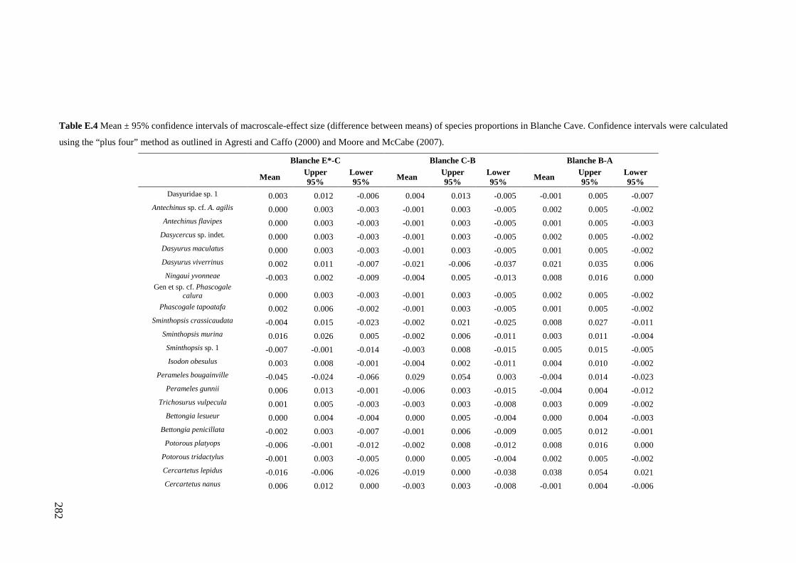
282
Table E.4 Mean ± 95% confidence intervals of macroscale-effect size (difference between means) of species proportions in Blanche Cave. Confidence intervals were calculated
using the “plus four” method as outlined in Agresti and Caffo (2000) and Moore and McCabe (2007).
Blanche E*-C Blanche C-B Blanche B-A
Mean Upper 95%
Lower 95% Mean Upper
95% Lower 95% Mean Upper
95% Lower 95%
Dasyuridae sp. 1 0.003 0.012 -0.006 0.004 0.013 -0.005 -0.001 0.005 -0.007 Antechinus sp. cf. A. agilis 0.000 0.003 -0.003 -0.001 0.003 -0.005 0.002 0.005 -0.002
Antechinus flavipes 0.000 0.003 -0.003 -0.001 0.003 -0.005 0.001 0.005 -0.003 Dasycercus sp. indet. 0.000 0.003 -0.003 -0.001 0.003 -0.005 0.002 0.005 -0.002 Dasyurus maculatus 0.000 0.003 -0.003 -0.001 0.003 -0.005 0.001 0.005 -0.002 Dasyurus viverrinus 0.002 0.011 -0.007 -0.021 -0.006 -0.037 0.021 0.035 0.006 Ningaui yvonneae -0.003 0.002 -0.009 -0.004 0.005 -0.013 0.008 0.016 0.000
Gen et sp. cf. Phascogale calura 0.000 0.003 -0.003 -0.001 0.003 -0.005 0.002 0.005 -0.002
Phascogale tapoatafa 0.002 0.006 -0.002 -0.001 0.003 -0.005 0.001 0.005 -0.002 Sminthopsis crassicaudata -0.004 0.015 -0.023 -0.002 0.021 -0.025 0.008 0.027 -0.011
Sminthopsis murina 0.016 0.026 0.005 -0.002 0.006 -0.011 0.003 0.011 -0.004 Sminthopsis sp. 1 -0.007 -0.001 -0.014 -0.003 0.008 -0.015 0.005 0.015 -0.005 Isodon obesulus 0.003 0.008 -0.001 -0.004 0.002 -0.011 0.004 0.010 -0.002
Perameles bougainville -0.045 -0.024 -0.066 0.029 0.054 0.003 -0.004 0.014 -0.023 Perameles gunnii 0.006 0.013 -0.001 -0.006 0.003 -0.015 -0.004 0.004 -0.012
Trichosurus vulpecula 0.001 0.005 -0.003 -0.003 0.003 -0.008 0.003 0.009 -0.002 Bettongia lesueur 0.000 0.004 -0.004 0.000 0.005 -0.004 0.000 0.004 -0.003
Bettongia penicillata -0.002 0.003 -0.007 -0.001 0.006 -0.009 0.005 0.012 -0.001 Potorous platyops -0.006 -0.001 -0.012 -0.002 0.008 -0.012 0.008 0.016 0.000
Potorous tridactylus -0.001 0.003 -0.005 0.000 0.005 -0.004 0.002 0.005 -0.002 Cercartetus lepidus -0.016 -0.006 -0.026 -0.019 0.000 -0.038 0.038 0.054 0.021 Cercartetus nanus 0.006 0.012 0.000 -0.003 0.003 -0.008 -0.001 0.004 -0.006
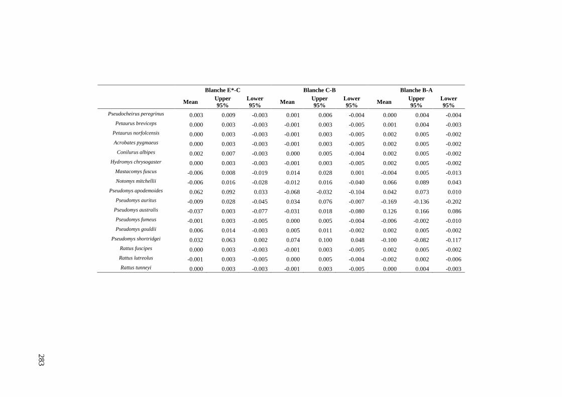
283
Blanche E*-C Blanche C-B Blanche B-A
Mean Upper 95%
Lower 95% Mean Upper
95% Lower 95% Mean Upper
95% Lower 95%
Pseudocheirus peregrinus 0.003 0.009 -0.003 0.001 0.006 -0.004 0.000 0.004 -0.004 Petaurus breviceps 0.000 0.003 -0.003 -0.001 0.003 -0.005 0.001 0.004 -0.003
Petaurus norfolcensis 0.000 0.003 -0.003 -0.001 0.003 -0.005 0.002 0.005 -0.002 Acrobates pygmaeus 0.000 0.003 -0.003 -0.001 0.003 -0.005 0.002 0.005 -0.002
Conilurus albipes 0.002 0.007 -0.003 0.000 0.005 -0.004 0.002 0.005 -0.002 Hydromys chrysogaster 0.000 0.003 -0.003 -0.001 0.003 -0.005 0.002 0.005 -0.002
Mastacomys fuscus -0.006 0.008 -0.019 0.014 0.028 0.001 -0.004 0.005 -0.013 Notomys mitchellii -0.006 0.016 -0.028 -0.012 0.016 -0.040 0.066 0.089 0.043
Pseudomys apodemoides 0.062 0.092 0.033 -0.068 -0.032 -0.104 0.042 0.073 0.010 Pseudomys auritus -0.009 0.028 -0.045 0.034 0.076 -0.007 -0.169 -0.136 -0.202
Pseudomys australis -0.037 0.003 -0.077 -0.031 0.018 -0.080 0.126 0.166 0.086 Pseudomys fumeus -0.001 0.003 -0.005 0.000 0.005 -0.004 -0.006 -0.002 -0.010 Pseudomys gouldii 0.006 0.014 -0.003 0.005 0.011 -0.002 0.002 0.005 -0.002
Pseudomys shortridgei 0.032 0.063 0.002 0.074 0.100 0.048 -0.100 -0.082 -0.117 Rattus fuscipes 0.000 0.003 -0.003 -0.001 0.003 -0.005 0.002 0.005 -0.002 Rattus lutreolus -0.001 0.003 -0.005 0.000 0.005 -0.004 -0.002 0.002 -0.006 Rattus tunneyi 0.000 0.003 -0.003 -0.001 0.003 -0.005 0.000 0.004 -0.003
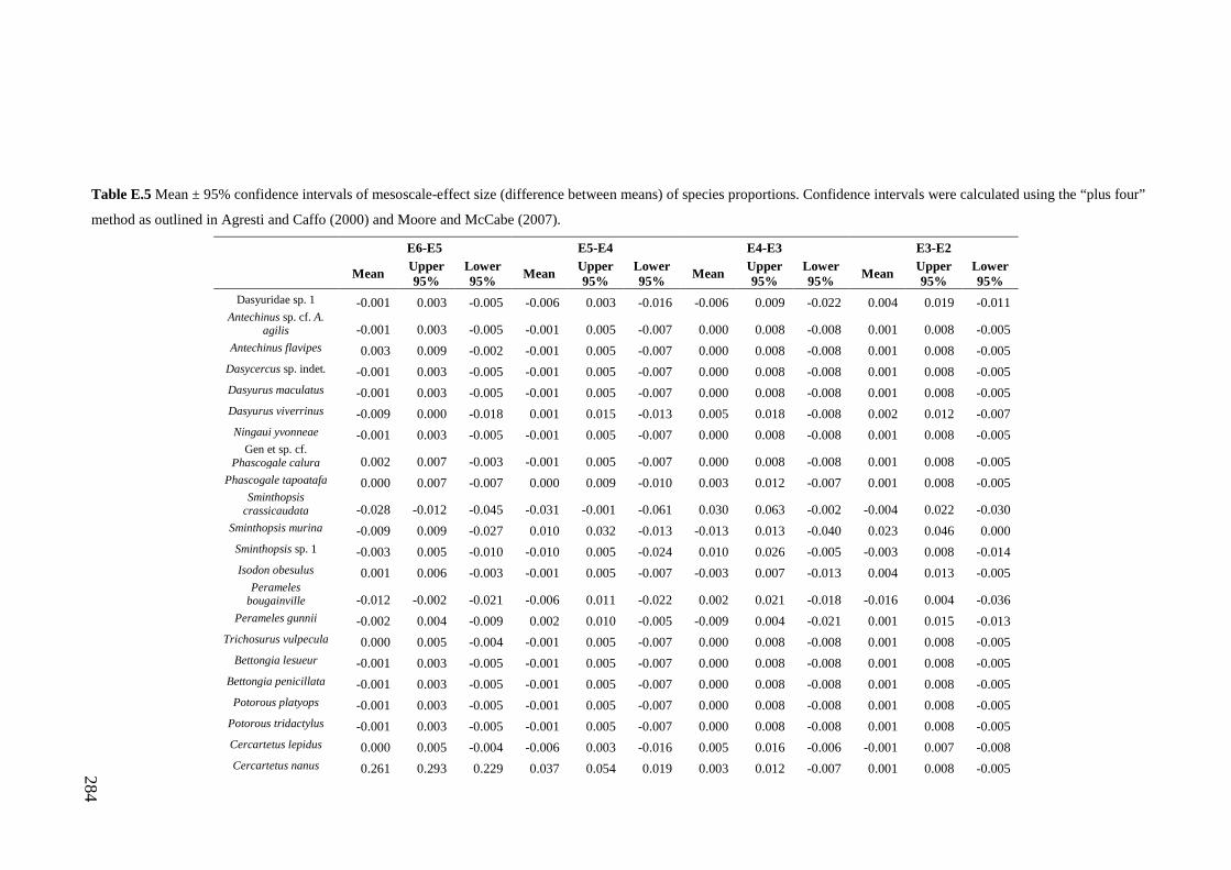
284
Table E.5 Mean ± 95% confidence intervals of mesoscale-effect size (difference between means) of species proportions. Confidence intervals were calculated using the “plus four”
method as outlined in Agresti and Caffo (2000) and Moore and McCabe (2007).
E6-E5 E5-E4 E4-E3 E3-E2
Mean Upper 95%
Lower 95% Mean Upper
95% Lower 95% Mean Upper
95% Lower 95% Mean Upper
95% Lower 95%
Dasyuridae sp. 1 -0.001 0.003 -0.005 -0.006 0.003 -0.016 -0.006 0.009 -0.022 0.004 0.019 -0.011 Antechinus sp. cf. A.
agilis -0.001 0.003 -0.005 -0.001 0.005 -0.007 0.000 0.008 -0.008 0.001 0.008 -0.005 Antechinus flavipes 0.003 0.009 -0.002 -0.001 0.005 -0.007 0.000 0.008 -0.008 0.001 0.008 -0.005
Dasycercus sp. indet. -0.001 0.003 -0.005 -0.001 0.005 -0.007 0.000 0.008 -0.008 0.001 0.008 -0.005 Dasyurus maculatus -0.001 0.003 -0.005 -0.001 0.005 -0.007 0.000 0.008 -0.008 0.001 0.008 -0.005 Dasyurus viverrinus -0.009 0.000 -0.018 0.001 0.015 -0.013 0.005 0.018 -0.008 0.002 0.012 -0.007 Ningaui yvonneae -0.001 0.003 -0.005 -0.001 0.005 -0.007 0.000 0.008 -0.008 0.001 0.008 -0.005
Gen et sp. cf. Phascogale calura 0.002 0.007 -0.003 -0.001 0.005 -0.007 0.000 0.008 -0.008 0.001 0.008 -0.005
Phascogale tapoatafa 0.000 0.007 -0.007 0.000 0.009 -0.010 0.003 0.012 -0.007 0.001 0.008 -0.005 Sminthopsis
crassicaudata -0.028 -0.012 -0.045 -0.031 -0.001 -0.061 0.030 0.063 -0.002 -0.004 0.022 -0.030 Sminthopsis murina -0.009 0.009 -0.027 0.010 0.032 -0.013 -0.013 0.013 -0.040 0.023 0.046 0.000
Sminthopsis sp. 1 -0.003 0.005 -0.010 -0.010 0.005 -0.024 0.010 0.026 -0.005 -0.003 0.008 -0.014 Isodon obesulus 0.001 0.006 -0.003 -0.001 0.005 -0.007 -0.003 0.007 -0.013 0.004 0.013 -0.005
Perameles bougainville -0.012 -0.002 -0.021 -0.006 0.011 -0.022 0.002 0.021 -0.018 -0.016 0.004 -0.036
Perameles gunnii -0.002 0.004 -0.009 0.002 0.010 -0.005 -0.009 0.004 -0.021 0.001 0.015 -0.013 Trichosurus vulpecula 0.000 0.005 -0.004 -0.001 0.005 -0.007 0.000 0.008 -0.008 0.001 0.008 -0.005
Bettongia lesueur -0.001 0.003 -0.005 -0.001 0.005 -0.007 0.000 0.008 -0.008 0.001 0.008 -0.005 Bettongia penicillata -0.001 0.003 -0.005 -0.001 0.005 -0.007 0.000 0.008 -0.008 0.001 0.008 -0.005
Potorous platyops -0.001 0.003 -0.005 -0.001 0.005 -0.007 0.000 0.008 -0.008 0.001 0.008 -0.005 Potorous tridactylus -0.001 0.003 -0.005 -0.001 0.005 -0.007 0.000 0.008 -0.008 0.001 0.008 -0.005 Cercartetus lepidus 0.000 0.005 -0.004 -0.006 0.003 -0.016 0.005 0.016 -0.006 -0.001 0.007 -0.008 Cercartetus nanus 0.261 0.293 0.229 0.037 0.054 0.019 0.003 0.012 -0.007 0.001 0.008 -0.005

285
Pseudocheirus peregrinus 0.001 0.006 -0.003 -0.004 0.004 -0.012 0.003 0.012 -0.007 0.001 0.008 -0.005
Petaurus breviceps 0.000 0.005 -0.004 -0.001 0.005 -0.007 0.000 0.008 -0.008 0.001 0.008 -0.005 Petaurus norfolcensis -0.002 0.003 -0.007 0.001 0.008 -0.006 0.000 0.008 -0.008 0.001 0.008 -0.005 Acrobates pygmaeus 0.042 0.057 0.028 0.002 0.010 -0.005 0.000 0.008 -0.008 0.001 0.008 -0.005
Conilurus albipes 0.010 0.017 0.003 -0.017 -0.003 -0.032 0.016 0.031 0.001 0.001 0.008 -0.005 Hydromys
chrysogaster -0.001 0.003 -0.005 -0.001 0.005 -0.007 0.000 0.008 -0.008 0.001 0.008 -0.005 Mastacomys fuscus -0.013 -0.003 -0.023 0.012 0.024 0.001 -0.023 -0.006 -0.041 0.009 0.028 -0.011 Notomys mitchellii -0.011 0.011 -0.033 -0.033 0.001 -0.067 0.046 0.082 0.011 0.007 0.033 -0.018
Pseudomys apodemoides 0.027 0.074 -0.020 0.098 0.153 0.043 -0.089 -0.026 -0.152 0.077 0.136 0.019
Pseudomys auritus -0.198 -0.164 -0.232 -0.104 -0.046 -0.162 0.083 0.148 0.017 -0.107 -0.047 -0.166 Pseudomys australis -0.111 -0.080 -0.141 -0.022 0.026 -0.069 0.009 0.063 -0.045 -0.014 0.036 -0.063 Pseudomys fumeus 0.017 0.026 0.008 -0.001 0.005 -0.007 0.000 0.008 -0.008 0.001 0.008 -0.005 Pseudomys gouldii 0.029 0.050 0.007 0.018 0.039 -0.003 -0.007 0.015 -0.029 0.014 0.033 -0.005
Pseudomys shortridgei -0.064 -0.041 -0.088 0.031 0.063 -0.001 -0.067 -0.026 -0.108 0.019 0.061 -0.023 Rattus fuscipes 0.035 0.048 0.023 0.001 0.008 -0.006 0.000 0.008 -0.008 0.001 0.008 -0.005 Rattus lutreolus 0.005 0.011 -0.001 -0.001 0.005 -0.007 0.000 0.008 -0.008 0.001 0.008 -0.005 Rattus tunneyi 0.009 0.019 -0.001 0.004 0.012 -0.004 0.000 0.008 -0.008 0.001 0.008 -0.005
E2-E1 E1-C2 C2-C1 C1-B1
Mean Upper
95% Lower 95% Mean Upper
95% Lower 95% Mean Upper
95% Lower 95% Mean Upper
95% Lower 95%
Dasyuridae sp. 1 0.004 0.016 -0.008 -0.005 0.008 -0.017 0.002 0.015 -0.012 0.004 0.016 -0.008 Antechinus sp. cf. A.
agilis -0.002 0.006 -0.009 0.002 0.009 -0.005 -0.002 0.005 -0.009 0.001 0.009 -0.006 Antechinus flavipes -0.002 0.006 -0.009 0.002 0.009 -0.005 -0.002 0.005 -0.009 0.001 0.009 -0.006
Dasycercus sp. indet. -0.002 0.006 -0.009 0.002 0.009 -0.005 -0.002 0.005 -0.009 0.001 0.009 -0.006 Dasyurus maculatus -0.002 0.006 -0.009 0.002 0.009 -0.005 -0.002 0.005 -0.009 0.001 0.009 -0.006 Dasyurus viverrinus -0.006 0.006 -0.018 0.000 0.014 -0.013 0.000 0.013 -0.013 -0.020 -0.002 -0.038
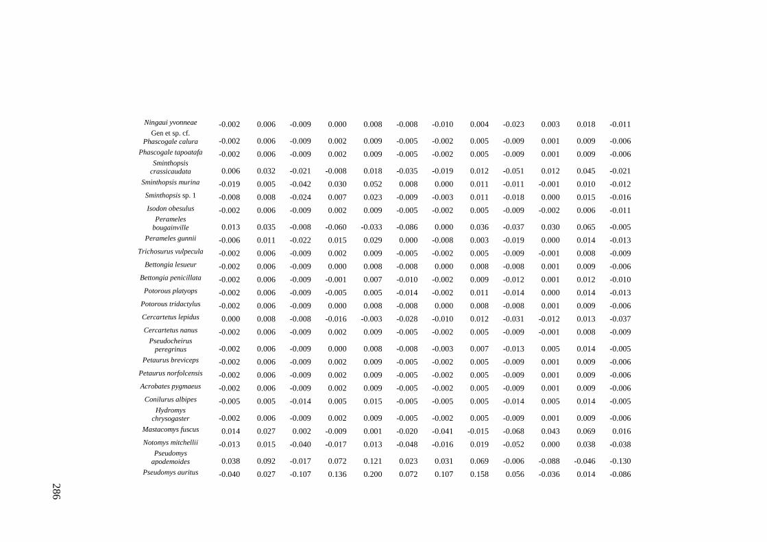
286
Ningaui yvonneae -0.002 0.006 -0.009 0.000 0.008 -0.008 -0.010 0.004 -0.023 0.003 0.018 -0.011 Gen et sp. cf.
Phascogale calura -0.002 0.006 -0.009 0.002 0.009 -0.005 -0.002 0.005 -0.009 0.001 0.009 -0.006 Phascogale tapoatafa -0.002 0.006 -0.009 0.002 0.009 -0.005 -0.002 0.005 -0.009 0.001 0.009 -0.006
Sminthopsis crassicaudata 0.006 0.032 -0.021 -0.008 0.018 -0.035 -0.019 0.012 -0.051 0.012 0.045 -0.021
Sminthopsis murina -0.019 0.005 -0.042 0.030 0.052 0.008 0.000 0.011 -0.011 -0.001 0.010 -0.012 Sminthopsis sp. 1 -0.008 0.008 -0.024 0.007 0.023 -0.009 -0.003 0.011 -0.018 0.000 0.015 -0.016 Isodon obesulus -0.002 0.006 -0.009 0.002 0.009 -0.005 -0.002 0.005 -0.009 -0.002 0.006 -0.011
Perameles bougainville 0.013 0.035 -0.008 -0.060 -0.033 -0.086 0.000 0.036 -0.037 0.030 0.065 -0.005
Perameles gunnii -0.006 0.011 -0.022 0.015 0.029 0.000 -0.008 0.003 -0.019 0.000 0.014 -0.013 Trichosurus vulpecula -0.002 0.006 -0.009 0.002 0.009 -0.005 -0.002 0.005 -0.009 -0.001 0.008 -0.009
Bettongia lesueur -0.002 0.006 -0.009 0.000 0.008 -0.008 0.000 0.008 -0.008 0.001 0.009 -0.006 Bettongia penicillata -0.002 0.006 -0.009 -0.001 0.007 -0.010 -0.002 0.009 -0.012 0.001 0.012 -0.010
Potorous platyops -0.002 0.006 -0.009 -0.005 0.005 -0.014 -0.002 0.011 -0.014 0.000 0.014 -0.013 Potorous tridactylus -0.002 0.006 -0.009 0.000 0.008 -0.008 0.000 0.008 -0.008 0.001 0.009 -0.006 Cercartetus lepidus 0.000 0.008 -0.008 -0.016 -0.003 -0.028 -0.010 0.012 -0.031 -0.012 0.013 -0.037 Cercartetus nanus -0.002 0.006 -0.009 0.002 0.009 -0.005 -0.002 0.005 -0.009 -0.001 0.008 -0.009
Pseudocheirus peregrinus -0.002 0.006 -0.009 0.000 0.008 -0.008 -0.003 0.007 -0.013 0.005 0.014 -0.005
Petaurus breviceps -0.002 0.006 -0.009 0.002 0.009 -0.005 -0.002 0.005 -0.009 0.001 0.009 -0.006 Petaurus norfolcensis -0.002 0.006 -0.009 0.002 0.009 -0.005 -0.002 0.005 -0.009 0.001 0.009 -0.006 Acrobates pygmaeus -0.002 0.006 -0.009 0.002 0.009 -0.005 -0.002 0.005 -0.009 0.001 0.009 -0.006
Conilurus albipes -0.005 0.005 -0.014 0.005 0.015 -0.005 -0.005 0.005 -0.014 0.005 0.014 -0.005 Hydromys
chrysogaster -0.002 0.006 -0.009 0.002 0.009 -0.005 -0.002 0.005 -0.009 0.001 0.009 -0.006 Mastacomys fuscus 0.014 0.027 0.002 -0.009 0.001 -0.020 -0.041 -0.015 -0.068 0.043 0.069 0.016 Notomys mitchellii -0.013 0.015 -0.040 -0.017 0.013 -0.048 -0.016 0.019 -0.052 0.000 0.038 -0.038
Pseudomys apodemoides 0.038 0.092 -0.017 0.072 0.121 0.023 0.031 0.069 -0.006 -0.088 -0.046 -0.130
Pseudomys auritus -0.040 0.027 -0.107 0.136 0.200 0.072 0.107 0.158 0.056 -0.036 0.014 -0.086
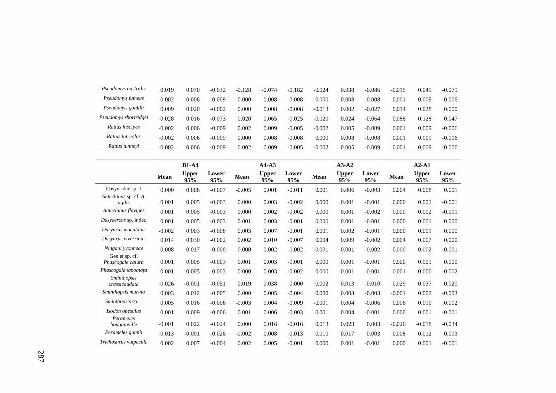
287
Pseudomys australis 0.019 0.070 -0.032 -0.128 -0.074 -0.182 -0.024 0.038 -0.086 -0.015 0.049 -0.079 Pseudomys fumeus -0.002 0.006 -0.009 0.000 0.008 -0.008 0.000 0.008 -0.008 0.001 0.009 -0.006 Pseudomys gouldii 0.009 0.020 -0.002 0.000 0.008 -0.008 -0.013 0.002 -0.027 0.014 0.028 0.000
Pseudomys shortridgei -0.028 0.016 -0.073 0.020 0.065 -0.025 -0.020 0.024 -0.064 0.088 0.128 0.047 Rattus fuscipes -0.002 0.006 -0.009 0.002 0.009 -0.005 -0.002 0.005 -0.009 0.001 0.009 -0.006 Rattus lutreolus -0.002 0.006 -0.009 0.000 0.008 -0.008 0.000 0.008 -0.008 0.001 0.009 -0.006 Rattus tunneyi -0.002 0.006 -0.009 0.002 0.009 -0.005 -0.002 0.005 -0.009 0.001 0.009 -0.006
B1-A4 A4-A3 A3-A2 A2-A1
Mean Upper
95% Lower 95% Mean Upper
95% Lower 95% Mean Upper
95% Lower 95% Mean Upper
95% Lower 95%
Dasyuridae sp. 1 0.000 0.008 -0.007 -0.005 0.001 -0.011 0.001 0.006 -0.003 0.004 0.008 0.001 Antechinus sp. cf. A.
agilis 0.001 0.005 -0.003 0.000 0.003 -0.002 0.000 0.001 -0.001 0.000 0.001 -0.001 Antechinus flavipes 0.001 0.005 -0.003 0.000 0.002 -0.002 0.000 0.001 -0.002 0.000 0.002 -0.001
Dasycercus sp. indet. 0.001 0.005 -0.003 0.001 0.003 -0.001 0.000 0.001 -0.001 0.000 0.001 0.000 Dasyurus maculatus -0.002 0.003 -0.008 0.003 0.007 -0.001 0.001 0.002 -0.001 0.000 0.001 0.000 Dasyurus viverrinus 0.014 0.030 -0.002 0.002 0.010 -0.007 0.004 0.009 -0.002 0.004 0.007 0.000 Ningaui yvonneae 0.008 0.017 0.000 0.000 0.002 -0.002 -0.001 0.001 -0.002 0.000 0.002 -0.001
Gen et sp. cf. Phascogale calura 0.001 0.005 -0.003 0.001 0.003 -0.001 0.000 0.001 -0.001 0.000 0.001 0.000
Phascogale tapoatafa 0.001 0.005 -0.003 0.000 0.003 -0.002 0.000 0.001 -0.001 -0.001 0.000 -0.002 Sminthopsis
crassicaudata -0.026 -0.001 -0.051 0.019 0.038 0.000 0.002 0.013 -0.010 0.029 0.037 0.020 Sminthopsis murina 0.003 0.012 -0.005 0.000 0.005 -0.004 0.000 0.003 -0.003 -0.001 0.002 -0.003
Sminthopsis sp. 1 0.005 0.016 -0.006 -0.003 0.004 -0.009 -0.001 0.004 -0.006 0.006 0.010 0.002 Isodon obesulus 0.001 0.009 -0.006 0.001 0.006 -0.003 0.001 0.004 -0.001 0.000 0.001 -0.001
Perameles bougainville -0.001 0.022 -0.024 0.000 0.016 -0.016 0.013 0.023 0.003 -0.026 -0.018 -0.034
Perameles gunnii -0.013 -0.001 -0.026 -0.002 0.008 -0.013 0.010 0.017 0.003 0.008 0.012 0.003 Trichosurus vulpecula 0.002 0.007 -0.004 0.002 0.005 -0.001 0.000 0.001 -0.001 0.000 0.001 -0.001
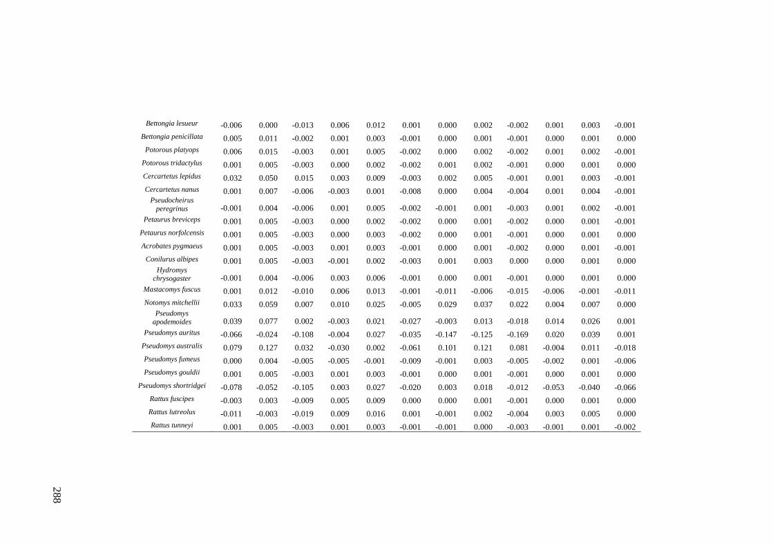
288
Bettongia lesueur -0.006 0.000 -0.013 0.006 0.012 0.001 0.000 0.002 -0.002 0.001 0.003 -0.001 Bettongia penicillata 0.005 0.011 -0.002 0.001 0.003 -0.001 0.000 0.001 -0.001 0.000 0.001 0.000
Potorous platyops 0.006 0.015 -0.003 0.001 0.005 -0.002 0.000 0.002 -0.002 0.001 0.002 -0.001 Potorous tridactylus 0.001 0.005 -0.003 0.000 0.002 -0.002 0.001 0.002 -0.001 0.000 0.001 0.000 Cercartetus lepidus 0.032 0.050 0.015 0.003 0.009 -0.003 0.002 0.005 -0.001 0.001 0.003 -0.001 Cercartetus nanus 0.001 0.007 -0.006 -0.003 0.001 -0.008 0.000 0.004 -0.004 0.001 0.004 -0.001
Pseudocheirus peregrinus -0.001 0.004 -0.006 0.001 0.005 -0.002 -0.001 0.001 -0.003 0.001 0.002 -0.001
Petaurus breviceps 0.001 0.005 -0.003 0.000 0.002 -0.002 0.000 0.001 -0.002 0.000 0.001 -0.001 Petaurus norfolcensis 0.001 0.005 -0.003 0.000 0.003 -0.002 0.000 0.001 -0.001 0.000 0.001 0.000 Acrobates pygmaeus 0.001 0.005 -0.003 0.001 0.003 -0.001 0.000 0.001 -0.002 0.000 0.001 -0.001
Conilurus albipes 0.001 0.005 -0.003 -0.001 0.002 -0.003 0.001 0.003 0.000 0.000 0.001 0.000 Hydromys
chrysogaster -0.001 0.004 -0.006 0.003 0.006 -0.001 0.000 0.001 -0.001 0.000 0.001 0.000 Mastacomys fuscus 0.001 0.012 -0.010 0.006 0.013 -0.001 -0.011 -0.006 -0.015 -0.006 -0.001 -0.011 Notomys mitchellii 0.033 0.059 0.007 0.010 0.025 -0.005 0.029 0.037 0.022 0.004 0.007 0.000
Pseudomys apodemoides 0.039 0.077 0.002 -0.003 0.021 -0.027 -0.003 0.013 -0.018 0.014 0.026 0.001
Pseudomys auritus -0.066 -0.024 -0.108 -0.004 0.027 -0.035 -0.147 -0.125 -0.169 0.020 0.039 0.001 Pseudomys australis 0.079 0.127 0.032 -0.030 0.002 -0.061 0.101 0.121 0.081 -0.004 0.011 -0.018 Pseudomys fumeus 0.000 0.004 -0.005 -0.005 -0.001 -0.009 -0.001 0.003 -0.005 -0.002 0.001 -0.006 Pseudomys gouldii 0.001 0.005 -0.003 0.001 0.003 -0.001 0.000 0.001 -0.001 0.000 0.001 0.000
Pseudomys shortridgei -0.078 -0.052 -0.105 0.003 0.027 -0.020 0.003 0.018 -0.012 -0.053 -0.040 -0.066 Rattus fuscipes -0.003 0.003 -0.009 0.005 0.009 0.000 0.000 0.001 -0.001 0.000 0.001 0.000 Rattus lutreolus -0.011 -0.003 -0.019 0.009 0.016 0.001 -0.001 0.002 -0.004 0.003 0.005 0.000 Rattus tunneyi 0.001 0.005 -0.003 0.001 0.003 -0.001 -0.001 0.000 -0.003 -0.001 0.001 -0.002

289
Table E.6 Chi-square statistics for Cochran’s test of linear trend for species proportions at the macroscale (units A, B, C and E) of Wet and Blanche Caves. Cochran’s test was
only performed on those species in Wet and Blanche which occurred within three or more units. 𝛘𝟐 is the normal chi-square test statistic which is divided into two components: 𝛘𝒕𝟐
is chi-square for linear trend; 𝛘𝒅𝟐 is chi-square for departure from linear trend (e.g., may be curvilinear). Significance assessed at α=0.01.
Cochran’s Test
Wet Cave Blanche Cave
Species 𝛘𝟐
(df = 3) p
𝛘𝒕𝟐
(df = 1) p
𝛘𝒅𝟐
(df = 2) p 𝛘𝟐
(df = 3) p
𝛘𝒕𝟐
(df = 1) p
𝛘𝒅𝟐
(df = 2) p
Dasyuridae sp. 1 2.417 0.490 0.870 0.351 0.275 0.872 4.598 0.204 3.070 0.080 1.528 0.466
Antechinus flavipes 5.763 0.124 4.078 0.043 1.685 0.431 Dasyurus viverrinus 26.791 0.000 14.485 0.000 12.306 0.002 20.780 0.000 0.422 0.516 20.359 0.000
Ningaui yvonneae 19.085 0.000 3.050 0.081 16.035 0.000
Sminthopsis crassicaudata 43.105 0.000 15.713 0.000 27.392 0.000 0.905 0.824 0.329 0.566 0.577 0.750
Sminthopsis murina 42.120 0.000 17.434 0.000 24.687 0.000 45.201 0.000 30.609 0.000 14.592 0.001
Sminthopsis sp. 1 0.640 0.887 0.167 0.682 0.473 0.789 6.558 0.087 2.820 0.093 3.738 0.154
Isoodon obesulus 12.524 0.006 0.696 0.404 11.829 0.003 4.772 0.189 0.473 0.492 4.299 0.117
Perameles bougainville 101.337 0.000 4.814 0.028 96.523 0.000 19.236 0.000 0.792 0.374 18.444 0.000
Perameles gunnii 31.227 0.000 29.919 0.000 1.308 0.520 11.264 0.010 7.585 0.006 3.679 0.159
Trichosurus vulpecula 7.652 0.054 2.083 0.149 5.570 0.062
Bettongia lesueur 1.145 0.766 0.478 0.489 0.667 0.716
Bettongia penicillata 40.105 0.000 18.420 0.000 21.685 0.000
Potorous platyops 16.421 0.001 0.177 0.674 16.244 0.000 23.050 0.000 2.006 0.157 21.044 0.000
Cercartetus lepidus 184.689 0.000 36.038 0.000 148.650 0.000
Cercartetus nanus 812.791 0.000 594.182 0.000 218.609 0.000 6.078 0.108 0.555 0.456 5.523 0.063
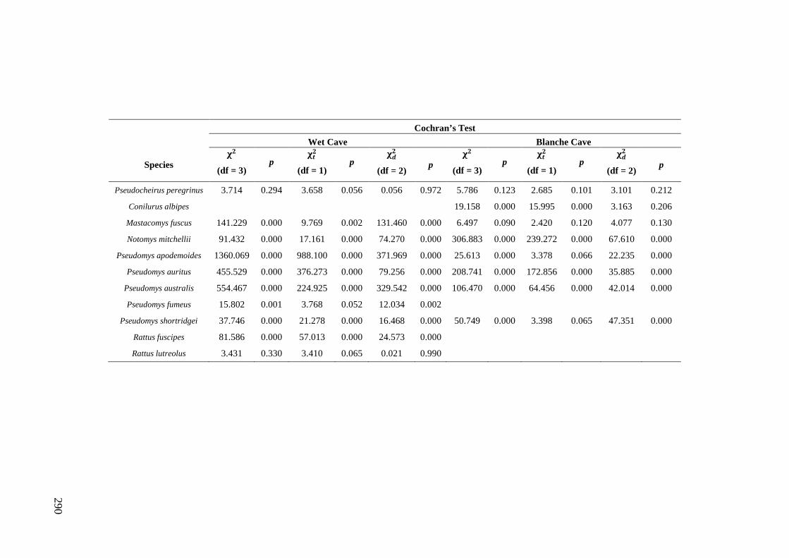
290
Cochran’s Test
Wet Cave Blanche Cave
Species 𝛘𝟐
(df = 3) p
𝛘𝒕𝟐
(df = 1) p
𝛘𝒅𝟐
(df = 2) p 𝛘𝟐
(df = 3) p
𝛘𝒕𝟐
(df = 1) p
𝛘𝒅𝟐
(df = 2) p
Pseudocheirus peregrinus 3.714 0.294 3.658 0.056 0.056 0.972 5.786 0.123 2.685 0.101 3.101 0.212
Conilurus albipes 19.158 0.000 15.995 0.000 3.163 0.206
Mastacomys fuscus 141.229 0.000 9.769 0.002 131.460 0.000 6.497 0.090 2.420 0.120 4.077 0.130
Notomys mitchellii 91.432 0.000 17.161 0.000 74.270 0.000 306.883 0.000 239.272 0.000 67.610 0.000
Pseudomys apodemoides 1360.069 0.000 988.100 0.000 371.969 0.000 25.613 0.000 3.378 0.066 22.235 0.000
Pseudomys auritus 455.529 0.000 376.273 0.000 79.256 0.000 208.741 0.000 172.856 0.000 35.885 0.000
Pseudomys australis 554.467 0.000 224.925 0.000 329.542 0.000 106.470 0.000 64.456 0.000 42.014 0.000
Pseudomys fumeus 15.802 0.001 3.768 0.052 12.034 0.002 Pseudomys shortridgei 37.746 0.000 21.278 0.000 16.468 0.000 50.749 0.000 3.398 0.065 47.351 0.000
Rattus fuscipes 81.586 0.000 57.013 0.000 24.573 0.000 Rattus lutreolus 3.431 0.330 3.410 0.065 0.021 0.990
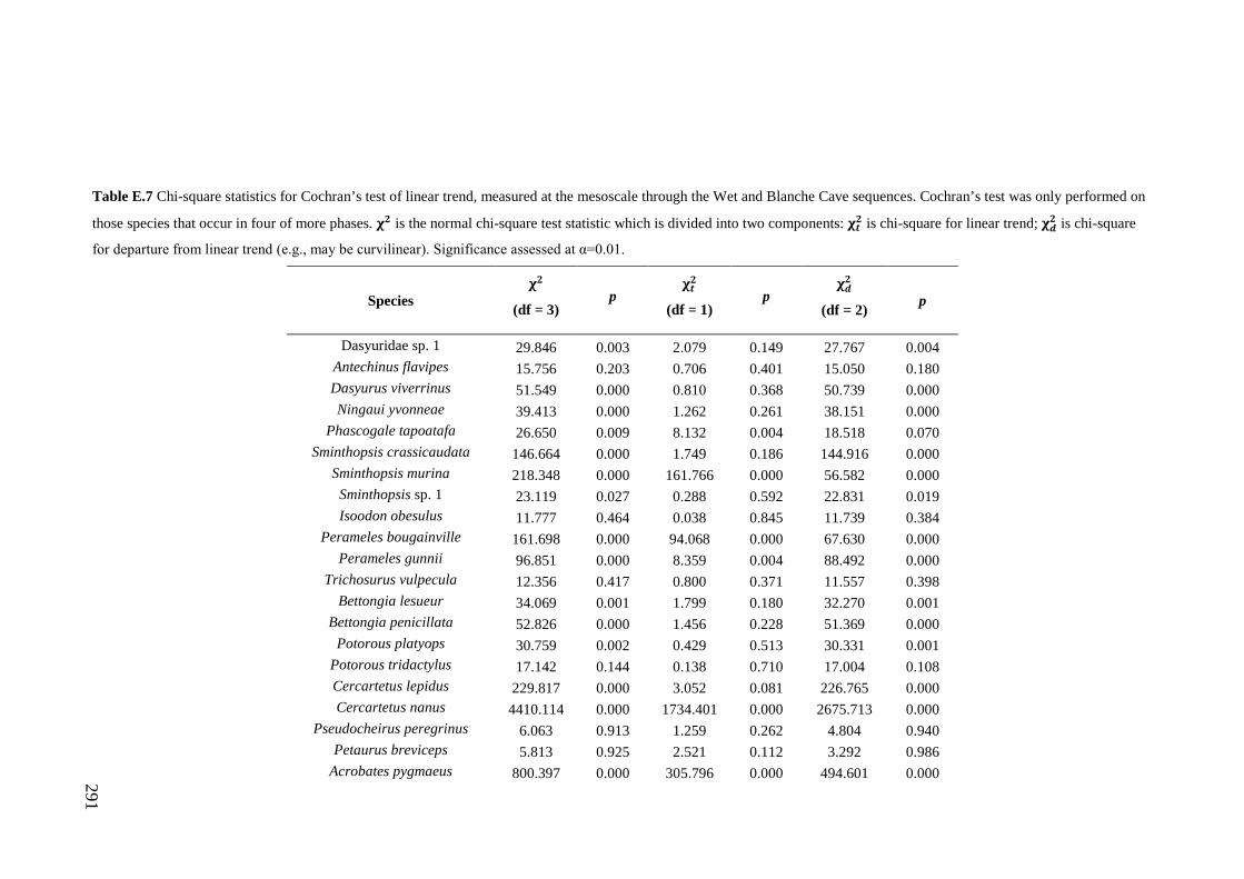
291
Table E.7 Chi-square statistics for Cochran’s test of linear trend, measured at the mesoscale through the Wet and Blanche Cave sequences. Cochran’s test was only performed on
those species that occur in four of more phases. 𝛘𝟐 is the normal chi-square test statistic which is divided into two components: 𝛘𝒕𝟐 is chi-square for linear trend; 𝛘𝒅𝟐 is chi-square
for departure from linear trend (e.g., may be curvilinear). Significance assessed at α=0.01.
Species 𝛘𝟐
(df = 3) p
𝛘𝒕𝟐
(df = 1) p
𝛘𝒅𝟐
(df = 2) p
Dasyuridae sp. 1 29.846 0.003 2.079 0.149 27.767 0.004 Antechinus flavipes 15.756 0.203 0.706 0.401 15.050 0.180 Dasyurus viverrinus 51.549 0.000 0.810 0.368 50.739 0.000 Ningaui yvonneae 39.413 0.000 1.262 0.261 38.151 0.000
Phascogale tapoatafa 26.650 0.009 8.132 0.004 18.518 0.070 Sminthopsis crassicaudata 146.664 0.000 1.749 0.186 144.916 0.000
Sminthopsis murina 218.348 0.000 161.766 0.000 56.582 0.000 Sminthopsis sp. 1 23.119 0.027 0.288 0.592 22.831 0.019 Isoodon obesulus 11.777 0.464 0.038 0.845 11.739 0.384
Perameles bougainville 161.698 0.000 94.068 0.000 67.630 0.000 Perameles gunnii 96.851 0.000 8.359 0.004 88.492 0.000
Trichosurus vulpecula 12.356 0.417 0.800 0.371 11.557 0.398 Bettongia lesueur 34.069 0.001 1.799 0.180 32.270 0.001
Bettongia penicillata 52.826 0.000 1.456 0.228 51.369 0.000 Potorous platyops 30.759 0.002 0.429 0.513 30.331 0.001
Potorous tridactylus 17.142 0.144 0.138 0.710 17.004 0.108 Cercartetus lepidus 229.817 0.000 3.052 0.081 226.765 0.000 Cercartetus nanus 4410.114 0.000 1734.401 0.000 2675.713 0.000
Pseudocheirus peregrinus 6.063 0.913 1.259 0.262 4.804 0.940 Petaurus breviceps 5.813 0.925 2.521 0.112 3.292 0.986
Acrobates pygmaeus 800.397 0.000 305.796 0.000 494.601 0.000
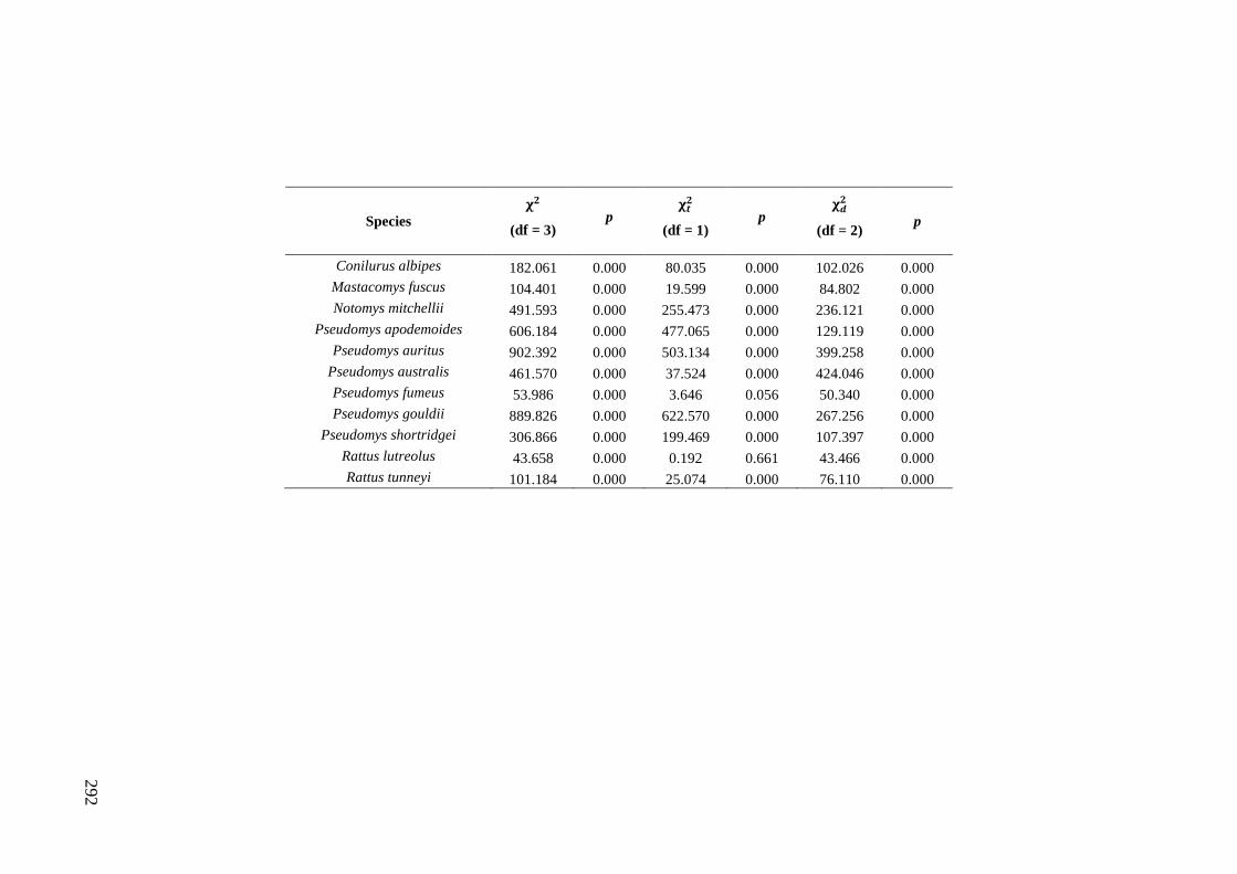
292
Species 𝛘𝟐
(df = 3) p
𝛘𝒕𝟐
(df = 1) p
𝛘𝒅𝟐
(df = 2) p
Conilurus albipes 182.061 0.000 80.035 0.000 102.026 0.000 Mastacomys fuscus 104.401 0.000 19.599 0.000 84.802 0.000 Notomys mitchellii 491.593 0.000 255.473 0.000 236.121 0.000
Pseudomys apodemoides 606.184 0.000 477.065 0.000 129.119 0.000 Pseudomys auritus 902.392 0.000 503.134 0.000 399.258 0.000
Pseudomys australis 461.570 0.000 37.524 0.000 424.046 0.000 Pseudomys fumeus 53.986 0.000 3.646 0.056 50.340 0.000 Pseudomys gouldii 889.826 0.000 622.570 0.000 267.256 0.000
Pseudomys shortridgei 306.866 0.000 199.469 0.000 107.397 0.000 Rattus lutreolus 43.658 0.000 0.192 0.661 43.466 0.000 Rattus tunneyi 101.184 0.000 25.074 0.000 76.110 0.000
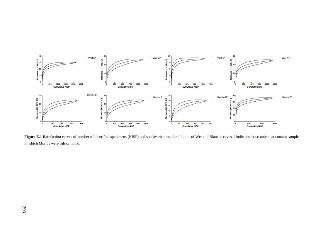
293
Figure E.1 Rarefaction curves of number of identified specimens (NISP) and species richness for all units of Wet and Blanche caves. ^Indicates those units that contain samples
in which Murids were sub-sampled.
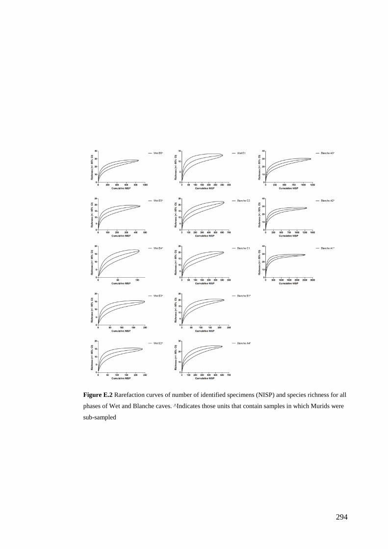
294
Figure E.2 Rarefaction curves of number of identified specimens (NISP) and species richness for all
phases of Wet and Blanche caves. ^Indicates those units that contain samples in which Murids were
sub-sampled
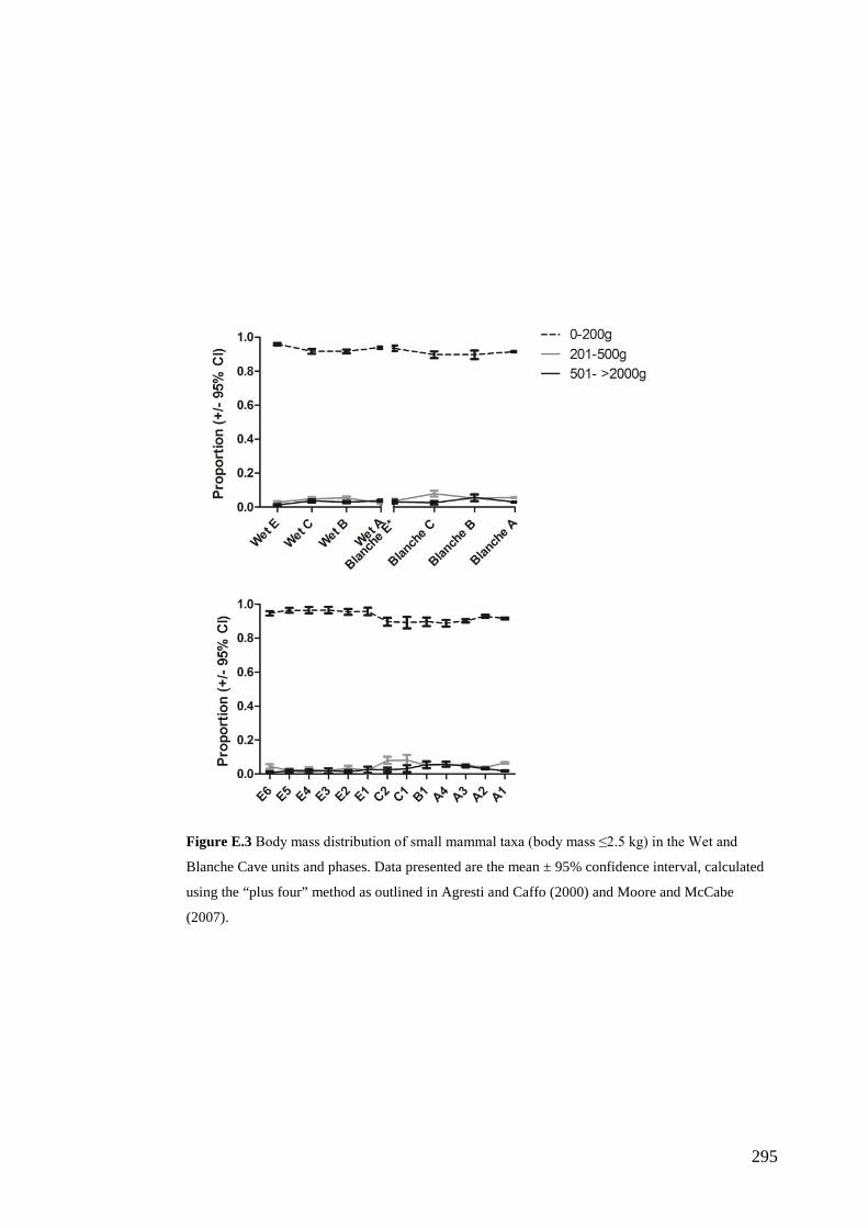
295
Figure E.3 Body mass distribution of small mammal taxa (body mass ≤2.5 kg) in the Wet and
Blanche Cave units and phases. Data presented are the mean ± 95% confidence interval, calculated
using the “plus four” method as outlined in Agresti and Caffo (2000) and Moore and McCabe
(2007).
296
Appendix F
Spatio-temporal distribution of Cercartetus concinnus
Contemporary (post-European arrival to present) The contemporary distribution of C. concinnus was compiled from records of
specimens held in Australian and international museums and research institutions
(Table F.1). Collection data were compiled from the Atlas of Living Australia
(ALA) database and were vetted against data supplied from the institutions directly.
The ALA also provided observational data, providing spatial occurrence points not
covered by the specimen records.
Spatial distribution maps were generated in ArcMap v10.1 (Fig. 7.1, main text).
Only specimens or observations in both the museum and ALA databases that had
latitude and longitudinal data were plotted in the distribution maps. Of the 2218
records of C. concinnus available across the combined museum and ALA database,
2115 had latitude and longitude reference points. Of these, 42 were marked as
‘spatially suspect,’ leaving 2073 data points for the distribution map.
C. concinnus is the most widespread of the pygmy possums in Australia, with a
distribution spanning southern Australia from south-west Western Australia to the
Murray mallee region of Victoria and New South Wales. The Nullarbor was
thought to form a barrier between eastern and western Australian populations,
providing support for Wakefield’s (1963) split of C. concinnus into two subspecies.
However, despite the lack of detection of C. concinnus in surveys of the Nullarbor
region in 1984 (McKenzie and Robinson, 1987), specimens were available from
this region for the phylogenetic analyses performed by Pestell et al. (2008). Harris
(2009) also noted specimens of C. concinnus collected from the Nullarbor Plain and
Great Victoria Desert, challenging the previous assumption of a disjunct
distribution of C. concinnus across southern Australia. Within the data compiled
from the ALA and museum collections, 219 records are associated with the
Nullarbor, Hampton and Great Victoria Desert Interim Biogeographic
Regionalisation for Australia (IBRA) regions. These records clearly verify the
297
presence of the species across this once considered distributional ‘gap.’ The records
associated with these regions were collected between 1974 and 2012.
Another interesting feature of the contemporary distribution of C. concinnus is the
history of its detection in the Murray Mallee region of south-western New South
Wales (NSW). The first record for C. concinnus in NSW was associated with a
specimen collected from near Gol Gol on the River Murray in 1958 (NMV C 2848).
A second specimen was collected from the Mallee Cliffs Conservation Park in 1996
(AM M32456), prompting the listing of C. concinnus as an endangered species in
NSW under the Threatened Species Conservation Act 1995.
Following its listing, a recovery plan was developed for C. concinnus in NSW and
surveys were conducted to determine the distribution and size of populations within
the state (NPWS, 2001). A total of 306 records of C. concinnus are available in the
combined museum and ALA database in the Murray Mallee region of NSW, dating
from 1996 to 2008.
Fossil (Pleistocene to Holocene) Quaternary-aged fossil occurrence data for C. concinnus were compiled from the
published literature. Latitude and longitudinal data for fossil localities were sourced
from the Geoscience Australia Place Name Search and published sources. Only a
limited number of fossil collections have been dated and in many cases, the
resolution of the dating prohibits fine-scale analysis of fossil occurrences with time.
As a result, the fossil distribution map was divided into the following time-periods:
1. Quaternary (2.6 myr to immediate pre-European arrival)
2. Pleistocene (2.6 myr to 11 kyr BP)
3. Late Pleistocene–Holocene (126 kyr to immediately pre-European arrival and/or
present day), and
4. Holocene (11 kyr to immediately pre-European arrival and/or present day).
Where minimum and/or maximum radiocarbon or other radiometric data were
available, these were used to constrain the specimens into one of these four time-
periods. For some sites, no dating was available but the age of the specimens was
inferred by the original authors through fossil association (e.g., presence of
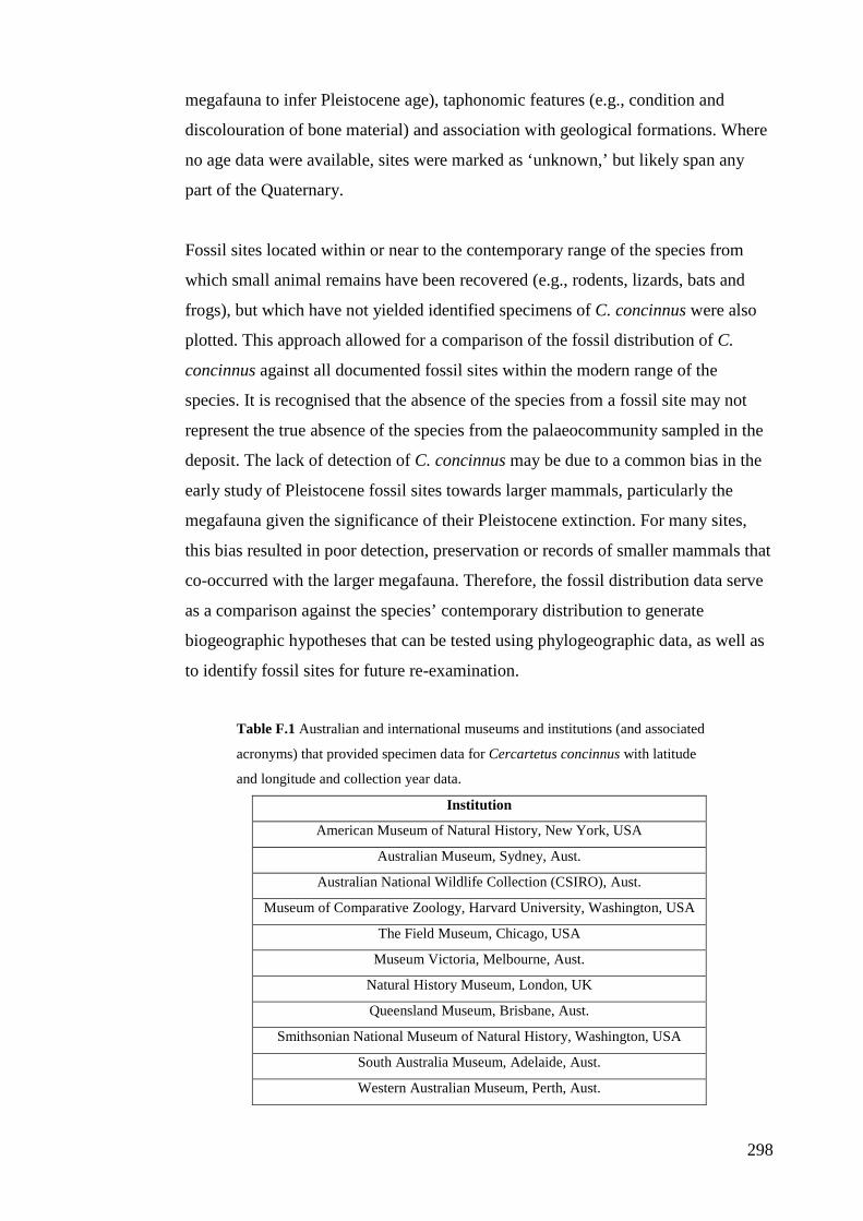
298
megafauna to infer Pleistocene age), taphonomic features (e.g., condition and
discolouration of bone material) and association with geological formations. Where
no age data were available, sites were marked as ‘unknown,’ but likely span any
part of the Quaternary.
Fossil sites located within or near to the contemporary range of the species from
which small animal remains have been recovered (e.g., rodents, lizards, bats and
frogs), but which have not yielded identified specimens of C. concinnus were also
plotted. This approach allowed for a comparison of the fossil distribution of C.
concinnus against all documented fossil sites within the modern range of the
species. It is recognised that the absence of the species from a fossil site may not
represent the true absence of the species from the palaeocommunity sampled in the
deposit. The lack of detection of C. concinnus may be due to a common bias in the
early study of Pleistocene fossil sites towards larger mammals, particularly the
megafauna given the significance of their Pleistocene extinction. For many sites,
this bias resulted in poor detection, preservation or records of smaller mammals that
co-occurred with the larger megafauna. Therefore, the fossil distribution data serve
as a comparison against the species’ contemporary distribution to generate
biogeographic hypotheses that can be tested using phylogeographic data, as well as
to identify fossil sites for future re-examination.
Table F.1 Australian and international museums and institutions (and associated
acronyms) that provided specimen data for Cercartetus concinnus with latitude
and longitude and collection year data.
Institution
American Museum of Natural History, New York, USA
Australian Museum, Sydney, Aust.
Australian National Wildlife Collection (CSIRO), Aust.
Museum of Comparative Zoology, Harvard University, Washington, USA
The Field Museum, Chicago, USA
Museum Victoria, Melbourne, Aust.
Natural History Museum, London, UK
Queensland Museum, Brisbane, Aust.
Smithsonian National Museum of Natural History, Washington, USA
South Australia Museum, Adelaide, Aust.
Western Australian Museum, Perth, Aust.
299
References Agresti, A. and Caffo, B. 2000. Simple and effective confidence intervals for
proportions and differences of proportions result from addition two successes
and two failures. The American Statistician 54, 280–288.
Alroy, J. 1999. Putting North America's end–Pleistocene megafaunal extinction in
context: large scale analyses of spatial patterns, extinction rates, and size
distributions. In: Extinctions in near time: causes, contexts, and
consequences. R.D.E. MacPhee (ed.), pp. 105–143. Plenum, New York.
Andrews, P. 1990. Owls, caves and fossils. University of Chicago Press, Chicago.
Andrews, P. and Lord, J.M. 1979. Patterns of ecological diversity in fossil and
modern mammalian fauna. Biological Journal of the Linnean Society 11,
177–205.
Aplin, K. and Archer, M. 1987. Recent advances in marsupial systematics with a
new syncretic classification. In: Possums and opossums: studies in evolution.
M. Archer (ed.), pp. xv–lxxii. Royal Zoological Society of New South Wales
and Surrey Beatty and Sons, New South Wales.
Archer, M. 1976. The Dasyurid dentition and its relationships to that of Didelphids,
Thylacinids, Borhyaenids (Marsupicarnivora) and Peramelids (Peramelina:
Marsupialia). Australian Journal of Zoology Supplementary Series 39, 1–34.
Armstrong, G. 2011. Evidence for the equal resilience of Triodia spp. Poaceae,
from different functional groups, to frequent fire dating back to the late
Pleistocene. Heredity 107, 558–564.
Armstrong, G. and Phillips, B. 2012. Fire history from life-history: determining the
fire regime that a plant community is adapted using life-histories. PLoS ONE
7, e31544.
Auler, A.S., Piló, L.B., Smart, P.L., Wang, X., Hoffmann, D., Richards, D.A.,
Edwards, R.L., Neves, W.A. and Cheng, H. 2006. U-series dating and
taphonomy of Quaternary vertebrates from Brazilian caves. Palaeogeography,
Palaeoclimatology, Palaeoecology 240, 508–522.
Ayliffe, L. and Veeh, H.H. 1988. Uranium-series dating of speleothems and bones
from Victoria Cave, Naracoorte, South Australia. Chemical Geology (Isotope
GeoScience Section) 72, 211–234.
Ayliffe, L.K., Marianelli, P.C., Moriarty, K.C., Wells, R.T., McCulloch, M.T.,
Mortimer, G.E. and Hellstrom, J.C. 1998. 500 ka precipitation record from
300
south-eastern Australia: evidence for interglacial relative aridity. Geology 26,
147–150.
Barnosky, A.D., Hadly, E.A. and Bell, C.J. 2003. Mammalian response to global
warming on varied temporal scales. Journal of Mammalogy 84, 354–368.
Barnosky, A.D., Koch, P.L., Feranec, R.S., Wing, S.L. and Shabel, A.B. 2004a.
Assessing the causes of late Pleistocene extinctions on the continents. Science
306, 70–75.
Barnosky, A.D., Bell, C.J., Emslie, S.D., Goodwin, H.T., Mead, J.I., Repenning,
C.A., Scott, E. and Shabel, A.B. 2004b. Exceptional record of mid-
Pleistocene vertebrates helps differentiate climatic from anthropogenic
ecosystem perturbations. Proceedings of the National Academy of Sciences
101, 9297–9302.
Barnosky, A.D. and Shabel A.B. 2005. Comparison of mammalian species richness
and community structure in historical and mid-Pleistocene times in the
Colorado Rocky Mountains. Proceedings of the Californian Academy of
Sciences 56, 50–61.
Barnosky, A.D., Carrasco, M.A. and Davis, E.B. 2005. The impact of the species-
area relationship on estimates of palaeodiversity. PLoS Biology 3, e266.
Barrows, T.T. and Juggins, S. 2005. Sea-surface temperatures around the Australian
margin and Indian Ocean during the last glacial maximum. Quaternary
Science Reviews 24, 1017–1047.
Barrows, T.T., Stone, J.O., Fifield, L.K. and Cresswell, R.G. 2001. Upper
Pleistocene glaciation of the Kosciuszko Massif, Snowy Mountains, Australia.
Quaternary Research 55, 179–189.
Barrows, T.T., Stone, J.O., Fifield, L.K. and Cresswell, R.G. 2002. The timing of
the last glacial maximum in Australia. Quaternary Science Reviews 21, 159–
173.
Bateman, B.L., Kutt, A.S., Vanderuys, E.P. and Kemp, J.E. 2010. Small-mammal
species richness and abundance along a tropical altitudinal gradient: an
Australian example. Journal of Tropical Ecology 26, 139–149.
Batterbee, R.W., Bennion, H., Gell, P. and Rose, N. 2011. Human impacts on
lacustrine ecosystems. In: The Sage Handbook of Environmental Change. J.A.
Matthews (ed.), pp. 583–606. SAGE Publication Ltd, California.
301
Baynes, A. and McDowell, M.C. 2010. The original fauna of the Pilbara
biogeographic region of north-western Australia. Records of the Western
Australian Museum Supplement 78, 285–298.
Bellingham, P.J., Towns, D.R., Cameron, E.K., Davis, J.J., Wardle, D.A.,
Wilmshurst, J.M. and Mulder, C.P.H. 2010. New Zealand island restoration:
seabirds, predators, and the importance of history. New Zealand Journal of
Ecology 34, 115–136.
Belmaker, M. and Hovers, E. 2011. Ecological change and the extinction of the
Levantine Neanderthals: implications from a diachronic study of
micromammals from Amud Cave, Israel. Quaternary Science Reviews 30,
3196–3209.
Belperio, A.P. 1995. Quaternary. In: The Geology of South Australia. The
Phanerozoic. J.F. Drexel and W.V. Preiss (eds.), pp. 219–280. Geological
Survey of South Australia, Bulletin no. 54, South Australian Department of
Mines.
Belyea, L.R. 2007. Revealing the Emperor’s new clothes: niche-based
palaeoenvironmental reconstruction in the light of recent ecological theory.
The Holocene 17, 683–688.
Bennington, J.B. and Bambach, R.K. 1996. Statistical testing for palaeocommunity
recurrence: are similar fossil assemblages ever the same? Palaeogeography,
Palaeoclimatology, Palaeoecology 127, 107–133.
Bennington, J.B., DiMichele, W.A., Badgley, C., Bambach, R.K., Barrett, P.M.,
Behrensmeyer, A.K., Bobe, R., Burnham, R., Baeschler, E.B., Van Dam, J.,
Eronen, J.T., Erwin, D.H., Finnegan, S., Holland, S.M., Hunt, G., Jablonski,
D., Jackson, S.T., Jacobs, B.F., Kidwell, S.M., Koch, P.L., Kowaleswski,
M.J., Labandeira, C.C., Looy, C.V., Lyons, S.K., Novack-Gottshall, P.M.,
Potts, R., Roopnarine, P.D., Ströberg, C.A.E., Sues, H., Wagner, P.J., Wilf, P.
and Wing, S. 2009. Critical issues of scale in paleoecology. Palaios 24, doi:
10.2110/palo.2009.S01.
Benton, M.J. 2009. The red queen and the court jester: species diversity and the role
of biotic and biotic factors through time. Science 323, 728–732.
Beramendi-Orosco, L.E., Gonzalez-Hernandez, G., Urrutia-Fucugauchi, J.,
Manzilla, L.R., Soler-Arechalde, A.M., Goguitchaishvili, A. and Jarboe, N.
2009. High-resolution chronology for the Mesoamerican urban centre of
302
Teotihuacan derived from Bayesian statistics of radiocarbon and
archaeological data. Quaternary Research 71, 99–107.
Bestland, E.A. and Rennie, J. 2006. Stable isotope record (δ 18O and δ13C) of a
Naracoorte Caves speleothem (Australia) from before and after the Last
Interglacial. Alcheringa Special Issue 1, 19–29.
Bilney, R.J., Cooke, R. and White, J.G. 2010. Underestimated and severe: small
mammal decline from the forests of south-eastern Australia since European
settlement, as revealed by a top-order predator. Biological Conservation 143,
52–59.
Birkland, P.W., Crandell, D.R. and Richmond, G.M. 1971. Status of correlation of
Quaternary stratigraphic units in the Western Conterminous United States.
Quaternary Research 1, 208–227.
Blaauw, M., Christen, J.A., Mauquoy, D., van der Plicht, J. and Bennett, K.D. 2007.
Testing the timing of radiocarbon-dated events between proxy archives. The
Holocene 17, 283–288.
Blockey, S.P.E. and Pinhasi, R. 2011. A revised chronology for the adoption of
agriculture in the Southern Levant and the role of Lateglacial climatic change.
Quaternary Science Reviews 30, 98–108.
Blois, J.L. and Hadly, E.A. 2009. Mammalian responses to Cenozoic climate
change. Annual Review of Earth and Planetary Science 37, 181–208.
Blois, J.L., McGuire, J.L. and Hadly, E.A. 2010. Small mammal diversity loss in
response to late-Pleistocene climatic change. Nature 465, 771–775.
Bobe, R., Behrensmeyer, A.K. and Chapman, R.E. 2002. Faunal change,
environmental variability and late Pliocene hominin evolution. Journal of
Human Evolution 42, 475-497.
Bureau of Meteorology 2013. Average Sea Surface Temperature Maps. Online:
http://www.bom.gov.au/climate/change/about/sst_averagemaps.shtml [viewed
6 June 2012].
Bowler, J.M. 1998. Willandra Lakes revisited: environmental framework for human
occupation. Archaeology in Oceania 33, 120–155.
Bowler, J.M., Kotsonis, A. and Lawrence, C.R. 2007. Environmental evolution of
the mallee region, western Murray Basin. Proceedings of the Royal Society of
Victoria 118, 161–210.
303
Bowler, J.M., Gillespie, R., Johnston, H. and Boljkovac, K. 2012. Wind v water:
glacial maximum records from the Willandra Lakes. Terra Australis 34, 271–
296.
Braithwait, R.W. and Muller, W.J. 1997. Rainfall, groundwater and refuges:
Predicting extinctions of Australian tropical mammal species. Australian
Journal of Ecology 22, 57–67.
Brenchly, P.J. and Harper, D.A.T. 1998. Paleoecology: ecosystems, environments
and evolution. Chapman and Horn, London.
Brennan, K.E.C., Christie, F.J. and York, A. 2009. Global climate change and litter
decomposition: more frequent fire slows decomposition and increases the
functional importance of invertebrates. Global Change Biology 15, 2958–
2971.
Bronk Ramsey, C. 1995. Radiocarbon calibration and analysis of stratigraphy: the
OxCal program. Radiocarbon 37, 425–430.
Bronk Ramsey, C. 2008. Depositional models for chronological records.
Quaternary Science Reviews 27, 42–60.
Bronk Ramsey, C. 2009a. Bayesian analysis of radiocarbon dates. Radiocarbon 51,
337–360.
Bronk Ramsey, C. 2009b. Dealing with outliers and offsets in radiocarbon dating.
Radiocarbon 51, 1023–1045.
Bronk Ramsey, C., Dee, M., Lee, S., Nakagawa, T. and Staff, R.A. 2010.
Developments in the calibration and modelling of radiocarbon dates.
Radiocarbon 52, 953–961.
Broughton, J.M., Byers, D.A., Bryson, R.A., Eckerle, W. and Madsen, D.B. 2008.
Did climatic seasonality control late Quaternary artiodactyl densities in
western North America? Quaternary Science Reviews 27, 1916–1937.
Brown, J.H. and Lomolino, W.V. 1998. Biogeography. 2nd edn. Sinaur Associates,
USA.
Brown, J.H., Melham, D.W. and Stevens, G.C. 1995. Spatial variation in
abundance. Ecology 76, 2028–2043.
Builth, H., Kershaw, A.P., White, C., Roach, A., Hartney, L., McKenzie, M., Lewis,
T. and Jacobsen, G. 2008. Environmental and cultural change on the Mt
Eccles lava-flow landscapes of southwest Victoria, Australia. The Holocene
18, 413–424.
304
Burbidge, A.A., McKenzie, N.L., Brennan, K.E.C., Woinarski, C., Dickman, C.R.,
Baynes, A., Gordon, G., Menkhorst, P.W. and Robinson, A.C. 2008.
Conservation status and biogeography of Australia’s terrestrial mammals.
Australian Journal of Zoology 56, 411–422.
Burney, D.A., James, H.F., Burney, L.P., Olson, S.L., Kikuchi, W., Wagner, W.L.,
Burney, M., McCloskey, D., Kikuchi, D., Grady, F.V., Gage II, R. and
Nishek, R. 2001. Fossil evidence for a diverse biota from Kaua’I and its
transformation since human arrival. Ecological Monographs 71, 615–641.
Byrne, M. 2008. Evidence for multiple refugia at different time scales during
Pleistocene climatic oscillations in southern Australia inferred from
phylogeography. Quaternary Science Reviews 27, 2576–2585.
Calcagnile, L., Tinè, V., Quarta, G., D’Elia, M., Fiorentino, G., Scarciglia, F.,
Robustelli, G., Abate, M., La Russa, M.F. and Pezzino, A. 2010.
Chronostratigraphic sequence of Santuario Della Madonna Cave (Calabria,
Southern Italy): AMS radiocarbon data from a new excavation area.
Radiocarbon 52, 408–414.
Calvo, E., Pelejero, C., De Deckker, P. and Logan, G.A. 2007. Antarctic deglacial
pattern in a 30 kyr record of sea surface temperature offshore South Australia.
Geophysical Research Letters 34, doi: 10.1029/2007GL029937.
Cannon M. 2000. Large mammal relative abundance in Pithouse and Pueblo Period
Archaeofaunas from southwestern New Mexico: resource depression among
the Mimbres-Mogollon? Journal of Anthropological Archaeology 19, 317–
347.
Cannon M. 2001. Archaeofaunal relative abundance, sample size and statistical
methods. Journal of Archaeological Science 28, 185–195.
Caran, S.C. 1998. Quaternary paleoenvironmental and paleoclimatic reconstruction:
a discussion and critique, with examples from the Southern High Plains.
Plains Anthropologist 43, 111–124.
Carrasco, M.A., Barnosky, A.D. and Graham, R.W. 2009. Quantifying the extent of
North American mammal extinction relative to the pre-anthropogenic
baseline. PLoS ONE 4, e8331.
Carrión, J.S., Lyll, E., Walker, M.J., Legaz, A.H., Chaín, C. and López, A. 2003.
Glacial refugia of temperate, Mediterranean and Ibero-North African flora in
305
south-eastern Spain: new evidence from cave pollen at two Neanderthal man
sites. Global Ecology and Biogeography 12, 119–129.
Ceballos, G., Arroyo-Cabrales, J., Ponce, E. 2010. Effects of Pleistocene
environmental changes on the distribution and community structure of the
mammalian fauna of Mexico. Quaternary Research 73, 464–473.
Chappell, J. 1991. Late Quaternary environmental changes in eastern and central
Australia, and their climatic interpretation. Quaternary Science Reviews 10,
377–390.
Chen, N. H., Bianchi, T. S., McKee, B. A. and Bland, J. M. 2001. Historical trends
of hypoxia on the Louisiana shelf: application of pigments as biomarkers.
Organic Geochemistry 32, 543–561.
Chernick, M.R. 2008. Bootstrap methods: a guide for practitioners and
researchers. 2nd edn. John Wiley and Sons, Inc., Hoboken, New Jersey.
Colhoun, E.A. 2000. Vegetation and climate change during the Last Interglacial –
Glacial cycle in western Tasmania, Australia. Palaeogeography,
Palaeoclimatology, Palaeoecology 155, 159–209.
Cook, E.J. 2009. A record of late Quaternary environments at lunette-lakes Bolac
and Turangmoroke, Western Victoria, Australia, based on pollen and a range
of non-pollen palynomorphs. Review of Paleobotany and Palynology 153,
185–224.
Cook, P.L.M., Holland, D.P. and Longmore, A.R. 2010. Effect of a flood event on
the dynamics of phytoplankton and biogeochemistry in a large temperate
Australian lagoon. Limnology and Oceanography 55, 1123–1133.
Cramb, J. and Hocknull, S. 2010. Two new species of Antechinus Macleay
(Dasyuridae: Marsupialia) from mid-Pleistocene cave deposits in eastern
central Queensland. Australian Mammalogy 32, 127–144.
Croft, T. 2003. Historical vegetation communities. In: A biological survey of the
south east of South Australia 1991 and 1997. J.N. Foulkes and L.M.B. Heard
(eds.), pp. 43–48. Department for Environment and Heritage, South Australia.
Crowly, B.E. 2010. A refined chronology of prehistoric Madagascar and the demise
of the megafauna. Quaternary Science Reviews 29, 2591–2603.
Crowther, M.S. 2002. Morphological variation within Antechinus agilis and
Antechinus stuartii (Marsupialia: Dasyuridae). Australian Journal of Zoology
50, 339–356.
306
Cuenca-Bescós, G., Straus, L.G., González Morales, M.R. and García Pimienta,
J.C. 2009. The reconstruction of past environments through small mammals:
from the Mousterian to the Bronze Age in El Mirón Cave (Cantabria, Spain).
Journal of Archaeological Science 36, 947–955.
Cumming, G. 2009. Inference by eye: reading the overlap of independent
confidence intervals. Statistics in Medicine 28, 205–220.
Cumming, G.S., Barnes, B., Perz, S., Schmink, M., Sieving, K.E., Southworth, J.,
Binford, M., Holt, R.D., Stickler, C. and Van Holt, T. 2005. An exploratory
framework for the empirical measurement of resilience. Ecosystems 8, 975–
987.
Cutler, K.B., Edwards, R.L., Taylor, F.W., Cheng, H., Adkins, J., Gallup, C.D.,
Cutler, P.M., Burr, G.S. and Bloom, A.L. 2003. Rapid sea-level fall and deep-
ocean temperature change since the last interglacial period. Earth and
Planetary Science Letters 206, 253–271.
Cuvier, G. 1817. Le Règne Animal distribué d’après son organisation, pour servir
de base a l’histoire naturelle des animaux et d’introduction a l’anatomie
compare. Déterville, Paris.
D’Costa, D. and Kershaw, A.P. 1997. An expanded recent pollen database from
south-eastern Australia and its potential for refinement of palaeoclimatic
estimates. Australian Journal of Botany 45, 583–605.
D’Costa, D.M., Edney, P., Kershaw, A.P. and De Deckker, P. 1989. Late
Quaternary paleoecology of Tower Hill, Victoria, Australia. Journal of
Biogeography 16, 461–482.
Dalby, L., Fox, A.D., Petersen, I.K., Delany, S. and Svenning, J. 2013. Temperature
does not dictate the wintering distributions of European dabbling duck
species. Ibis 155, 80–88.
Darrénougué, N., De Deckker, P., Fitzsimmons, K.E., Norman, M.D., Reed, L., van
der Kaars, S. and Fallon, S. 2009. A late Pleistocene record of aeolian
sedimentation in Blanche Cave, Naracoorte, South Australia. Quaternary
Science Reviews 28, 2600–2615.
Davies, T.J., Purvis, A. and Glitterman, J.L. 2009. Quaternary climate change and
the geographic ranges of mammals. The American Naturalist 174, 297–307.
Davis, J., Froend, R., Hamilton, D., Horwitz, P., McComb, A., Oldham, C. and
Thomas, D. 2001. Environmental water requirements to maintain wetlands of
307
national and international importance. Environmental Flows Initiative
Technical Report Number 1. Commonwealth of Australia, Canberra.
Davis, S.R., Brown, A.G. and Dinnin, M.H. 2007. Floodplain connectivity,
disturbance and change: a palaeoentomological investigation of floodplain
ecology from south-west England. Journal of Animal Ecology 76, 276–288.
Demarshelier, J.M., Goede, A., Ayliffe, L.K., McCulloch, M.T. and Moriarty, K.
2000. Stable isotope record and its palaeoenvironmental interpretation for a
late Middle Pleistocene speleothem from Victoria Fossil Cave, Naracoorte,
South Australia. Quaternary Science Reviews 19, 763–774.
Department for Environment and Heritage and South East Natural Resource
Management Board. Gliders of the South East. Online:
http://www.senrm.sa.gov.au/LinkClick.aspx?fileticket=geabJ__nPNw%3Dan
dtabid=400andmid=1297. [viewed 23 Oct 2011].
DeSantis, L.R.G., Feranec, R.S. and MacFadden, B.J. 2009. Effects of global
warming on ancient mammalian communities and their environments. PLoS
ONE 4, e5750.
Devictor, V. and Robert, A. 2009. Measuring community responses to large-scale
disturbance in conservation biogeography. Diversity and Distributions 15,
122–130.
Di Stefano, J. 2004. A confidence interval approach to data analysis. Forest
Ecology and Management 187, 173–183.
Dickman, C.R., Parnaby, H.E., Crowther, M.S. and King, D.H. 1998. Antechinus
agilis (Marsupialia: Dasyuridae), a new species from the A. stuartii complex
in south-eastern Australia. Australian Journal of Zoology 46, 1–26.
Dietl, G.P. and Flessa, K.W. 2011. Conservation Paleobiology: putting the dead to
work. Trends in Ecology and Evolution 26, 30–37.
DiMichele, W.A., Behrensmeyer, A.K., Olszewski, T.D., Labandeira, C.C.,
Pandolfi, J.M., Wing, S.L. and Bobe, R. 2004. Long-term stasis in ecological
assemblages: evidence from the fossil record. Annual Review of Ecology,
Evolution and Systematics 35, 285–322.
Dodson, J.R. 1975. Vegetation history and water fluctuations at Lake Leake, south-
eastern South Australia. II 50,000 B.P. to 10,000 B.P. Australian Journal of
Botany 23, 815–831.
308
Dodson, J.R. 1977. Late Quaternary palaeoecology of Wyrie Swamp, south-eastern
South Australia. Quaternary Research 8, 97–114.
Dodson, J.R. and Mooney, S.D. 2002. An assessment of historic human impact on
south-eastern Australian environmental systems, using late Holocene rates of
environmental change. Australian Journal of Botany 50, 455–464.
Dodson, J.R. and Ono, Y. 1997. Timing of late Quaternary vegetation response in
the 30-50° latitude bands in south-eastern Australia and northeastern Asia.
Quaternary International 37, 89–104.
du Toit, J.T. 2010. Considerations of scale in biodiversity conservation. Animal
Conservation 13, 229–236.
Erwin, D. 2009. A call to the custodians of deep time. Nature 462, 282–283.
Excoffier, L. and Ray, N. 2008. Surfing during population expansions promotes
genetic revolutions and structuration. Trends in Ecology and Evolution 23,
347–351.
Farrand, W.R. 2001. Sediments and stratigraphy in rockshelters and caves: a
personal perspective on principles and pragmatics. Geoarchaeology 16, 537–
557.
Fernandez-Jalvo, Y. and Andrews. P. 1992. Small mammal taphonomy of Gran
Dolina Atapuerca (Burgos), Spain. Journal of Archaeological Science 19,
407–428.
Finney, B.P., Alheit, J., Emeis, K.C., Field, D.B., Guiérrez, D. and Struck, U. 2010.
Paleoecological studies on variability in marine fish populations: A long-term
perspective on the impacts of climate change on marine ecosystems. Journal
of Marine Systems 79, 316–326.
Fitzimmons, K.E., Rhodes, E.J., Magee, J.W. and Barrows, T.T. 2007. The timing
of linear dune activity in the Strzelecki and Tirari deserts, Australia.
Quaternary Science Reviews 26, 2598–2616.
Folke, C., Carpenter, S., Walker, B., Scheffer, M., Elmqvist, T., Gunderson, L. and
Holling, C.S. 2004. Regime shifts, resilience, and biodiversity in ecosystem
management. Annual Review of Ecology, Evolution and Systematics 35, 557–
581.
Forbes, M.S. and Bestland, E.A. 2006. Guano-derived deposits within the sandy
cave fills of Naracoorte, South Australia. Alcheringa Special Issue 1, 129–
146.
309
Forbes, M.S. and Bestland, E.A. 2007. Origin of the sedimentary deposits of the
Naracoorte Caves, South Australia. Geomorphology 86, 369–392.
Forbes, M.S., Bestland, E.A., Wells, R.T. and Krull, E.S. 2007.
Palaeoenvironmental reconstruction of the Late Pleistocene to Early Holocene
Robertson Cave sedimentary deposit, Naracoorte, South Australia. Australian
Journal of Earth Sciences 54, 541–559.
Foster, D.R., Orwig, D.A. and McLachlan, J.S. 1996. Ecological and conservation
insights from reconstructive studies of temperate old-growth forests. Trends
in Ecology and Evolution 11, 419–424.
Foulkes, J.N. and Heard, L.M. (eds.) 2003. A biological survey of the South East,
South Australia. 1991 and 1997. Department of Environment and Heritage,
South Australia.
Foulkes, J.N., Owens, H., Croft, T. and Carpenter, G. 2003a. Mammals. In: A
biological survey of the south east of South Australia 1991 and 1997. J.N.
Foulkes and L.M. Heard (eds.), pp. 193–225. Department of Environment and
Heritage, South Australia.
Foulkes, J.N., Owens, H., Croft, T. and Carpenter, G. 2003b. Reptiles. In: A
biological survey of the south east of South Australia 1991 and 1997. J.N.
Foulkes and L.M. Heard (eds.), pp. 273–329. Department of Environment and
Heritage, South Australia.
Fraser, R.A. and Wells, R.T. 2006. Palaeontological excavation and taphonomic
investigation of the late Pleistocene fossil deposit in Grant Hall, Victoria
Fossil Cave, Naracoorte, South Australia. Alcheringa Special Issue 1, 147–
161.
Froyd, C.A. and Willis, K.J. 2008. Emerging issues in biodiversity and conservation
management: the need for a palaeoecological perspective. Quaternary Science
Reviews 27, 1723–1732.
Frumkin, A., Kadan, G., Enzel, Y. and Eyal, Y. 2001. Radiocarbon chronology of
the Holocene Dead Sea: attempting a regional correlation. Radiocarbon 43,
1179–1189.
Gammage, B. 2011. Fire in 1788: the closest ally. Australian Historical Studies 42,
277–288.
Gell, P. 2010. With the benefit of hindsight: the utility of palaeoecology in wetland
condition assessment and identification of restoration targets. In: Ecology of
310
industrial pollution. L.C. Batty and K.B. Hallberg (eds.), pp. 162–188.
Cambridge University Press, New York.
Gell, P.A., Barker, P.A., De Deckker, P., Last, W.M. and Jelicic, L. 1994. The
Holocene history of West Basin Lake, Victoria, Australia; chemical changes
based on fossil biota and sediment mineralogy. Journal of Paleolimnology 12,
235–258.
Geoffroy, St H.E. 1796. Dissertation sur les animaux à bourse Didelphis, L.
Magasin Encyclopaedique 3, 445–472.
Gill, T. 1872. Arrangement of the families of mammals. With analytical tables.
Smithsonian Institute, Washington.
Gillespie, R. 2002. Dating the first Australians. Radiocarbon 44, 455–472.
Goldfuss, G.A. 1820. Handbuch der Zoologie. Johann Leonhard Schrag,
Nürenburg.
Gorham, E., Brush, G.S., Graumlich, L.J., Rosenzweig, M.L., Johnson, A.H. 2001.
The value of paleoecology as an aid to monitoring ecosystems and
landscapes, chiefly with reference to North America. Environmental Reviews
9, 99–126.
Gott, B. 2005. Aboriginal fire management in south-eastern Australia: aims and
frequency. Journal of Biogeography 32, 1203–1208.
Gould, J. 1844. Exhibition and character of a number of animals transmitted from
Australia by Mr Gilbert. Proceedings of the Zoological Society of London 12,
103.
Graham, R.W. 1985. Diversity and community structure of the late Pleistocene
mammal fauna of North America. Acta Zoological Fennica 170, 181–192.
Graham, R.W. and Grimm, E.C. 1990. Effects of global climate change on the
patterns of terrestrial biological communities. Trends in Ecology and
Evolution 5, 289–292.
Graham, R.W., Lundelius Jr, E.L., Graham, M.A., Schroeder, E.K., Toomey III,
R.S., Anderson, E,. Barnosky, A.D., Burns, J.A., Churcher, C.S., Grayson,
D.K., Guthrie, R.D., Harington, C.R., Jefferson, G.T., Martin, L.D.,
McDonald, H.G., Morlan, R.E., Semken Jr, H.A., Webb, S.D., Werdelin, L.
and Wilson, M.C. 1996. Spatial response of mammals to Late Quaternary
Environmental Fluctuations. Science 272, 1601–1606.
311
Green, K., Stein, J.A. and Driessen, M.M. 2008. The projected distributions of
Mastacomys fuscus and Rattus lutreolus in south-eastern Australia under a
scenario of climate change: potential for increased competition? Wildlife
Research 35, 113–119.
Groffman, P.M., Baron, J.S., Blett, T., Gold, A.J., Goodman, I., Gunderson, L.H.,
Levinson, B.M., Palmer, M.A., Paerl, H.W., Peterson, G.D., Poff, N.L.,
Rejeski, D.W., Reynolds, J.F., Turner, M.G., Weathers, K.C. and Wiens, J.
2006. Ecological thresholds: the key to successful environmental management
or an important concept with no practical application? Ecosystems 9, 1–13.
Grün, R., Moriarty, K. and Wells, R. 2001. Electron spin resonance dating of the
fossil deposits in the Naracoorte Caves, South Australia. Journal of
Quaternary Science 16, 49–59.
Grundell, R., Gell, P. and Mills, K. 2012. Interaction between a river and its
wetland: evidence from the Murray River for spatial variability in diatom and
radioisotope records. Journal of Paleolimnology 47, 205–219.
Hadly, E.A. 1999. Fidelity of terrestrial vertebrate fossils to a modern ecosystem.
Palaeogeography, Palaeoclimatology, Palaeoecology 149, 389–409.
Hadly, E.A. and Barnosky, A.D. 2009. Vertebrate fossils and the future of
Conservation Biology. In: Conservation Paleobiology. using the past to
manage for the future. G.P. Dietl and K.W. Flessa (eds.), pp. 39–59. The
Palaeontological Society Papers 15.
Hadly, E.A., Spaeth, P.A. and Li, C. 2009. Niche conservatism above the species
level. Proceedings of the National Academy of Sciences106, 19707–19714.
Hammer, O. and Harper, D. 2006. Paleontological Data Analysis. Blackwell
Publishing, United Kingdom.
Hammer, O., Harper, D.A.T. and Ryan, P.D. 2001. PAST: Paleontological statistics
software package for education and data analysis. Palaeontologica
Electronica 4, 1–9.
Harle, K.J. 1997. Late Quaternary vegetation and climatic change in southeastern
Australia: palynological evidence from marine core E55-6. Palaeogeography,
Palaeoclimatology, Palaeoecology 131, 465–483.
Harle, K.J., Heijnis, H., Chisari, R., Kershaw, A.P., Zoppi, U. and Jacobsen, G.
2002. A chronology for the long pollen record from Lake Wangoom, western
312
Victoria (Australia) as derived from uranium/thorium disequilibrium dating.
Journal of Quaternary Science 17, 707–720.
Harris, J.M. 2006. Fossil occurrences of Cercartetus nanus (Marsupialia:
Burramyidae) in South Australia. Transactions of the Royal Society of South
Australia 131, 239–244.
Harris, J.M. 2009a. Cercartetus concinnus (Diprotodontia: Burramyidae).
Mammalian Species 831, 1–11.
Harris, J.M. 2009b. Cercartetus lepidus (Diprotodontia: Burramyidae). Mammalian
Species 842, 1–8.
Harris, J.M. and Garvey, J.M. 2006. Palaeodistribution of Pygmy-possums in
Tasmania. Papers and Proceedings of the Royal Society of Tasmania 140, 1–
10.
Harris, J.M. and Goldingay, R.L. 2005. The distribution of fossil and sub-fossil
records of the Eastern Pygmy-possum Cercartetus nanus in Victoria. The
Victorian Naturalist 122, 160–170.
Harris, J.M. and Moloney, K.S. 2010. Petauroides volans (Diprotodontia:
Pseudocheiridae). Mammalian Species 42, 207–219.
Hearty, P.J., Olson, S.L., Kaufman, D.S., Edwards, R.L. and Cheng, H. 2004.
Stratigraphy and geochronology of pitfall accumulations in caves and fissures,
Bermuda. Quaternary Science Reviews 23, 1151–1171.
Heller, N.E. and Zavaleta, E.S. 2009. Biodiversity management in the face of
climate change: A review of 22 years of recommendations. Biological
Conservation 142, 14–32.
Hernández Fernández, M and Peláez-Campomanes, P 2005. Quantitative
palaeoclimatic inference based on terrestrial mammal faunas. Global Ecology
and Biogeography 14, 39–56.
Hesse. P., Magee, J.W. and van der Kaars, S. 2004. Late Quaternary climates of the
Australian arid zone. Quaternary International 118–119, 87–102.
Higham, T., Jacobi, R., Julien, M., David, F., Basell, L., Wood, R., Davies, W. and
Bronk Ramsey, C. 2010. Chronology of the Grotte du Renne (France) and
implications for the context of ornaments and human remains within the
Châtelperronian. Proceedings of the National Academy of Sciences 107,
20234–20239.
313
Hocknull, S.A., Zhao, J., Feng, Y. and Webb, G.E. 2007. Responses of Quaternary
rainforest vertebrates to climate change in Australia. Earth and Planetary
Science Letters 264, 317–331.
Holling, C.S. 1996. Engineering resilience versus ecological resilience. In:
Engineering within ecological constraints. P.C. Shultz (ed.), pp. 31–44.
National Academy Press, USA.
Holling, C.S. and Meffe, G.K. 1996. Command and control and the pathology of
natural resource management. Conservation Biology 10, 328–337.
Hopley, P.J. and Maslin, M.A. 2010. Climate-averaging of terrestrial faunas: an
example from the Plio-Pleistocene of South Africa. Paleobiology 36, 32–50.
Hopton, D. 2003. Climate. In: A biological survey of the south east of South
Australia 1991 and 1997. J.N. Foulkes and L.M.B. Heard (eds.), pp. 13–15.
Department for Environment and Heritage, South Australia.
IBM Corp. 2010. IBM SPSS Statistics for Windows, Version 19.0. Armonk, New
York.
Illigeri, C. 1811. Prodromus systematis mammalium et avium additis terminis
zoographicis utriusque classis, eorumque versione Germanica. Bertolini
Sumptibus C. Salfeld.
Jackson, S.T. and Sax, D.F. 2010. Balancing biodiversity in a changing
environment: extinction debt, immigration credit and species turnover. Trends
in Ecology and Evolution 25, 153–160.
Jackson, D.A., Walker, S.C. and Poos, M.S. 2010. Cluster analysis of fish
community data: “new” tools for determining meaningful groupings of sites
and relative abundance of species. American Fisheries Society Symposium 73,
503–527.
Jacobi, R.M. and Higham, T.F.G. 2009. The early Lateglacial re-colonisation of
Britain: new radiocarbon evidence from Gough’s Cave, southwest England.
Quaternary Science Reviews 28, 1895–1913.
Jones, R. 1969. Firestick farming. Australian Natural History 16, 224–228.
Jones, R. N., McMahon, T. A. and Bowler, J. M. 2001. Modelling historical lake
levels and recent climate change at three closed lakes, western Victoria,
Australia c. 1840-1990. Journal of Hydrology 246, 159–180.
Jouzel, J., Vaikmae, R., Petit, J.R., Martin, M., Duclos, Y., Stievenard, M., Lorius,
C., Toots, M., Mélières, M.A., Burckle, L.H., Barkov, N.I. and Kotlyakov,
314
V.M. 1995. The two-step shape and timing of the last deglaciation in
Antarctica. Climate Dynamics 11, 151–161.
Kannan, E. and James, D.A. 2009. Effects of climate change on global biodiversity:
a review of key literature. Tropical Ecology 50, 31–39.
Keith, S.A., Newton, A.C., Herbert, R.J.H., Morecroft, M.D. and Bealey, C.E.
2009. Non-analogous community formation in response to climate change.
Journal for Nature Conservation 17, 228–235.
Kelly, L.T., Nimmo, D.G., Spence-Bailey, L.M., Clarke, M. and Bennett, A.F.
2010. The short-term responses of small mammals to wildfire in semiarid
mallee shrubland, Australia. Wildlife Research 37, 293–300.
Kemp, J. and Spooner, N.A. 2007. Evidence for regionally wet conditions before
the LGM in southeast Australia: OSL ages from a large paleochannel in the
Lachlan Valley. Journal of Quaternary Science 22, 423–427.
Kemp, J., Radke, L.C., Olley, J., Juggins, S. and De Deckker, P. 2012. Holocene
lake salinity changes in the Wimmera, southeastern Australia, provide
evidence for millennial-scale climate variability. Quaternary Research 77,
65–76.
Kemper, C., Medlin, G. and Bachmann, M. 2010. The discovery and history of the
heath mouse Pseudomys shortridgei (Thomas, 1907) in South Australia.
Transactions of the Royal Society of South Australia 134, 125–138.
Kerr, R. 1792. The animal kingdom, or zoological system, of the celebrated Sir
Charles Linnaeus; class 1. Mammalia; being a translation of that part of the
Systema Naturae, as lately published with great improvements by Professor
Gmelin, together with numerous additions from more recent zoological
writers and illustrated with copperplates. J. Murray, London.
Kershaw, P., Moss, P. and van der Kaars, S. 2003. Causes and consequences of
long-term climatic variability on the Australian continent. Freshwater Biology
48, 1274–1283.
Kershaw, A.P., Tibby, J., Penny, D., Yezdani, H., Walkley, R., Cook, E.J. and
Johnston, R. 2004. Latest Pleistocene and Holocene vegetation and
environmental history of the Western Plains of Victoria, Australia.
Proceedings of the Royal Society of Victoria 116, 139–161.
Kidwell, S.M. 2001. Preservation of species abundance in marine death
assemblages. Science 294, 1091–1094.
315
Kidwell, S.M. and Flessa, K.W. 1996. The quality of the fossil record: populations,
species and communities. Annual Review of Earth and Planetary Science 24,
433–464.
Koch, P.L. and Barnosky, A.D. 2006. Late Quaternary extinctions: state of the
debate. Annual Review of Ecology, Evolution and Systematics 37, 215–250.
Kos, A.M. 2001. Stratigraphy, sedimentary development and paleoenvironmental
context of a naturally accumulated pitfall cave deposit from south-eastern
Australia. Australian Journal of Earth Sciences 48, 621–632.
Kuhner, M. K. 2009. Coalescent genealogy samplers: windows into population
history. Trends in Ecology and Evolution 24, 86–93.
Landres, P.B., Morgan, P. and Swanson, F.J. 1999. Overview of the use of natural
variability concepts in managing ecological systems. Ecological Applications
9, 1179–1188.
Laslett, T.M. 2006. A palaeoecological study of a Quaternary vertebrate fossil
deposit in Blanche Cave, Naracoorte, South Australia. B.Sc. (Hons.) Thesis,
Flinders University, Australia.
Leavitt, P. R. and Hodgson, D. A. 2001. Sedimentary pigments. In: Tracking
environmental change using lake sediments. J. P. Smol, H. J. B. Birks and W.
M. Last (eds.), pp. 295–325. Kluwer Academic Publishers, Dordrecht.
Lepetz, V., Massot, M., Schmeller, D.S. and Clobert, J. 2009. Biodiversity
monitoring: some proposals to adequately study species’ responses to climate
change. Biodiversity Conservation 18, 3185–3203.
Lewis, I.D., Lawrence, R. and Mott, K. 2006. Origin and genesis of the major caves
at Naracoorte, South Australia. Conference abstract. IGCP 448 Global karst
correlation and the first international workshop on RAMSAR subterranean
wetlands. Naracoorte, October 2004. Helictite 39, 55–75.
Li, Q., McGowran, B. and White, M.R. 2000. Sequences and biofacies packages in
the mid-Cenozoic Gambier Limestone, South Australia: reappraisal of
foraminiferal evidence. Australian Journal of Earth Sciences 47, 955–970.
Lockley, M.G. 1977. The application of ecological theory to palaeoecological
studies, with special reference to equilibrium theory and the Ordovician
System. Lethaia 11, 281–291.
316
Lomax J., Hilgers A. and Radtke U. 2011. Paleoenvironmental change recorded in
the paleodunefields of the western Murray Basin, South Australia – New data
from single grain OSL-dating. Quaternary Science Reviews 30, 723–736.
Lomolino, M.V. 2000. Ecology's most general, yet protean pattern: the species-area
relationship. Journal of Biogeography 27, 17–26.
Lopes dos Santos, R.A., Wilkins, D., De Deccker, P. and Schouten, S. 2012. Late
Quaternary productivity changes from offshore South-eastern Australia: a
biomarker approach. Palaeogeography, Palaeoclimatology, Palaeoecology
363–364, 48–56.
Lowe, J.J. and Walker, M.J.C. 1997. Reconstructing Quaternary environments. 2nd
edn. Prentice Hall, United Kingdom.
Luckett, P.W. 1993. An ontogenetic assessment of dental homologies in Therian
mammals. In: Mammal Phylogeny: Mesozoic differentiation, Multituberates,
Monotremes, early Therians and Marsupials. F.S. Szalay, M.J. Novalek and
M.C. McKenna (eds.), pp. 192–204. Springer-Verlag, New York.
Ludbrook, N.H. 1961. Stratigraphy of the Murray Darling Basin in South Australia.
Geological Survey of South Australia, Bulletin no. 36, South Australian
Department of Mines.
Lundberg, P., Ranta, E., Ripa, J. and Kaitala, V. 2000. Population variability in
space and time. Trends in Ecology and Evolution 15, 460–464.
Lundelius Jr, E.L. 1964. The use of vertebrates in paleoecological reconstructions.
In: The Reconstruction of Past Environments, Fort Burgwin Conference on
Paleoecology 3, 26–30 (Hester, J.J. and Schoenwetter, J.).
Lundelius Jr, E.L. 1989. The implications of disharmonious assemblages for
Pleistocene extinctions. Journal of Archaeological Science 16, 407–417.
Lundelius Jr, E.L., and Turnbull, W.D. 1978. The mammalian fauna of Madura
Cave, Western Australia Part III. Fieldiana Geology 38, 1–140.
Lyman, R.L. 2006. Paleozoology in the service of conservation biology.
Evolutionary Anthropology 15, 11–19.
Lyman, R.L. 2008. Quantitative Paleozoology. Cambridge University Press, New
York.
MacDonald, G.M., Bennett, K.D., Jackson, S.T., Parducci, L., Smith, F.A., Smol,
J.P. and Willis, K.J. 2008. Impacts of climate change on species, populations
317
and communities: palaeobiogeographical insights and frontiers. Progress in
Physical Geography 32, 139–172.
Macken, A.C. 2009. Palaeoecological investigation of the Grant Hall fossil deposit,
Victoria Fossil Cave, Naracoorte, South Australia. BSc Hons Thesis. Flinders
University of South Australia, Australia.
Macken, A.C. and Reed, E.H. 2013. Late Quaternary small mammal faunas of the
Naracoorte Caves World Heritage Area. Transactions of the Royal Society of
South Australia 137, 53–67.
Macken, A.C., Jankowski, N.R., Price, G.P., Bestland, E.A., Reed, E.H., Prideaux,
G.P. and Roberts, R.G. 2011. Application of sedimentary and chronological
analyses to refine the depositional context of a Late Pleistocene vertebrate
deposit, Naracoorte, South Australia. Quaternary Science Reviews 30, 2690–
2702.
Macken, A.C., Prideaux, G.J. and Reed, E.H. 2012. Variation and pattern in the
responses of mammal faunas to Late Pleistocene climatic change in
southeastern South Australia. Journal of Quaternary Science 27, 415–424.
Macken, A.C., McDowell, M.C., Bartholomeusz, D.H. and Reed, E.H. 2013a.
Chronology and stratigraphy of the Wet Cave vertebrate fossil deposit,
Naracoorte, and relationship to palaeoclimatic conditions of the Last Glacial
Cycle in south-eastern Australia. Australian Journal of Earth Sciences 60,
271–281.
Macken, A.C., Staff, R.A. and Reed, E.H. 2013b. Bayesian age-depth modelling of
Late Quaternary deposits from Wet and Blanche caves, Naracoorte, South
Australia: a framework for comparative faunal analyses. Quaternary
Geochronology 17, 26–43.
Mackintosh, A.N., Barrows, T.T., Colhoun, E.A. and Fifield, L.K. 2006. Exposure
dating and glacial reconstruction at Mt. Field, Tasmania, Australia, identified
MIS 3 and MIS 2 glacial advances and climatic variability. Journal of
Quaternary Science 21, 363–376.
Macleay, W.S. 1841. Notice of a new genus of Mammalia discovered by J. Stuart,
Esq., in New South Wales. Annals and Magazine of Natural History 8, 241–
243.
Magee, J.W., Bowler, J.M., Miller, G.H. and Williams, D.L.G. 1995. Stratigraphy,
sedimentology, chronology and palaeohydrology of Quaternary lacustrine
318
deposits at Madigan Gulf, Lake Eyre, South Australia. Palaeogeography,
Palaeoclimatology, Palaeoecology 113, 3–42.
Magurran, A.E. and Henderson, P.E. 2010. Temporal turnover and the maintenance
of diversity in ecological assemblages. Philosophical Transactions of the
Royal Society B 365, 3611–3620.
Manning, A.D., Fischer, J., Felton, A., Newell, B., Steffen, W. and Lindenmayer,
D.B. 2009. Landscape fluidity – a unifying perspective for understanding and
adapting to global change. Journal of Biogeography 36, 193–199.
Marini, A.M., Barbet-Massin, M., Lopes, L.E. and Jiguet, F. 2009. Predicted
climate-driven bird distribution changes and forecasted conservation conflicts
in a neotropical savanna. Conservation Biology 23, 1558–1567.
Martinson, D.G., Pisias, N.G., Hays, J.D., Imbrie, J., Moore, T.C. and Shackleton,
N.J. 1987. Age dating and the orbital theory of the ice ages: development of a
high-resolution 0 to 300,000-year chronostratigraphy. Quaternary Research
27, 1–29.
Matthews, P.G. 1985. Australian Karst Index. 4th edn. Australian Speleothem
Federation. Online: http://www.caves.org.au/downloads/STDMAP.pdf.
[Viewed 6 February 2012].
McCormac, F.G., Hogg, A.G., Blackwell, P.G., Buck, C.E., Higham, T.F.G. and
Reimer, P.J. 2004. SHCal04 Southern Hemisphere calibration, 0-11.0 cal kyr
BP. Radiocarbon 46, 1087–1092.
McDowell, M.C. 2001. The analysis of Late Quaternary fossil mammal faunas from
Robertson Cave (5U17, 18, 19) and Wet Cave (5U10, 11) in the Naracoorte
World Heritage Area, South Australia. M.Sc. Thesis, Flinders University,
Australia.
McDowell, M.C. and Medlin, G.C. 2009. The effects of drought on prey selection
of the barn owl Tyto alba in the Strzelecki Regional Reserve, north-eastern
South Australia. Australian Mammalogy 31, 47–55.
McDowell, M.C. and Medlin, G.C. 2010. Natural resource management
implications of the pre-European non-volant mammal fauna of the southern
tip of Eyre Peninsula, South Australia. Australian Mammalogy 32, 87–93.
McDowell, M.C., Baynes, A., Medlin, G.C. and Prideaux, G.J. 2012. The impact of
European colonization on the late Holocene non-volant mammals of Yorke
Peninsula, South Australia. The Holocene 22, 1441–1450.
319
McDowell, M.C., Bestland, E.A., Bertuch, F., Ayliffe, L.K., Hellstrom, J.C.,
Jacobsen, G.E. and Prideaux, G.J. 2013. Chronology, stratigraphy and
palaeoenvironmental interpretation of a Late Pleistocene to mid-Holocene
cave accumulation on Kangaroo Island, South Australia. Boreas, In Press.
McKenzie, N.L. and Robinson, A.C. (eds.) 1987. A Biological Survey of the
Nullarbor Region South and Western Australia in 1984. South Australian
Department of Environment and Planning, Western Australian Department of
Conservation and Land Management and Australian National Parks and
Wildlife Service.
McKinney, M.L. 1997. Extinction vulnerability and selectivity: combining
ecological and paleontological views. Annual Review of Ecological Systems
28, 495–516.
Meyeneck, J. 2004. Effects of global climate change on geographic distributions of
vertebrates in North Queensland. Ecological Modelling 74, 347–357.
Micheli, F., Cottingham, K.L., Bascompte, J., Bjornstad, O.N., Eckert, G.L.,
Fischer, J.M., Keitt, T.H., Kendall, B.E., Klug, J.L. and Rusak, J.A. 1999. The
dual nature of community variability. Oikos 85, 161–169.
Mooney, S.D., Harrison, S.P., Bartlein, P.J., Daniau, A-L., Stevenson, J., Brownlie,
K.C., Buckman, S., Cupper, M., Luly, J., Black, M., Colhoun, E., D’Costa,
D., Dodson, J., Haberle, S., Hope, G.S., Kershaw, P., Kenyon, C., McKenzie,
M. and Williams, N. 2011. Late Quaternary fire regimes of Australasia.
Quaternary Science Reviews 30, 28–46.
Moore, D.S. and McCabe, G.P. 2007. Introduction to the Practice of Statistics. 5th
edn. W.H. Freeman and Company. New York, USA.
Moriarty, K.C., McCulloch, M.T., Wells, R.T. and McDowell, M.C. 2000. Mid-
Pleistocene cave fills, megafaunal remains and climate change at Naracoorte,
South Australia: towards a predictive model using U-Th dating of
speleothems. Palaeogeography, Palaeoclimatology, Palaeoecology 159, 113–
145.
Moss, P.T., Thomas, I. and Macphail, M. 2007. Late Holocene vegetation and
environments of the Mersey Valley, Tasmania. Australian Journal of Botany
55, 74–82.
320
Munguía, M., Townsend, P. and Sánchez-Cordero, V. 2008. Dispersal limitation
and geographical distributions of mammal species. Journal of Biogeography
35, 1879–1887.
Murray-Wallace, C.V., Brooke, B.P., Cann, J.H., Belperio, A.P. and Bourman, R.P.
2001. Whole-rock aminostratigraphy of the Coorong Coastal Plain, South
Australia: towards a 1 million year record of sea-level highstands. Journal of
the Geological Society 158, 111–124.
Nakagawa, S. 2004. A farewell to Bonferroni: the problems of low statistical power
and publication bias. Behavioural Ecology 15, 1044–1045.
Nakagawa, S. and Cuthill, I. 2007. Effect size, confidence interval and statistical
significance: a practical guide for biologists. Biological Reviews 82, 591–605.
Nanson, G.C., Cohen, T.J., Doyle, C.J. and Price, D.M. 2003. Alluvial evidence of
major late-Quaternary climate and flow-regime changes on the coastal rivers
of New South Wales, Australia. In: Paleohydrology: Understanding Global
Change. Gregory K.J. and Benito G. (eds), pp. 233–271. John Wiley and
Sons, West Sussex, UK.
National Biodiversity Strategy Review Task Group (NBSRTG) 2009. Australia’s
Biodiversity Conservation Strategy 2010–2020 Consultation Draft.
Department of the Environment, Water, Heritage and the Arts, Canberra,
Australian Capital Territory.
Nielsen-Marsh, C.M. 2000. Patterns of diagenesis in bone I: the effects of site
environments. Journal of Archaeological Science 27, 1139–1150.
North, M. and Stine, P. 2012. Clarifying Concepts. In: Managing Sierra Nevada
Forests. General Technical Report PSW-GTR-237. M. North (ed.), pp. 149–
164. U.S. Department of Agriculture, Forest Service, Pacific Southwest
Research Station, California.
Ogden, R.W. 2000. Modern and historical variation in aquatic macrophyte cover of
billabongs associated with catchment development. Regulated Rivers:
Research and Management 16, 487–512.
Osborne, M.J. and Christidis, L. 2002. Systematics and biogeography of pygmy-
possums (Burramyidae: Cercartetus). Australian Journal of Zoology 50, 25–
37.
321
Page, K., Nanson, G. and Price, D. 1996. Chronology of Murrumbidgee River
paleochannels on the Riverine Plain, south-eastern Australia. Journal of
Quaternary Science 11, 311–326.
Page K.J., Dare-Edwards A.J., Owens J.W., Frazier P.S., Kellett J. and Price D.M.
2001. TL chronology and stratigraphy of riverine source bordering sand dunes
near Wagga Wagga, New South Wales, Australia. Quaternary International
83–85, 187–193.
Page K.J., Kemp J. and Nanson G.C. 2009. Late Quaternary evolution of the
Riverine Plain paleochannels, south-eastern Australia. Australian Journal of
Earth Sciences 56, S19–S33.
Pahnke, K., Zahn, R., Elderfield, H., and Schulz, M. 2003. 340,000-year centennial-
scale marine record of Southern Hemisphere climatic oscillation. Science 301,
948–952.
Parmesan, C. and Yohe, G. 2003. A globally coherent fingerprint of climate change
impacts across natural systems. Nature 421, 37–42.
Parnell, A.C., Buck, C.E. and Doan, T.K. 2011. A review of statistical chronology
models for high-resolution, proxy based Holocene palaeoenvironmental
reconstruction. Quaternary Science Reviews 30, 2948–2960.
Pate, F.D., McDowell, M.C., Wells, R.T. and Smith, A.M. 2002. Last recorded
evidence for megafauna at Wet Cave, Naracoorte, South Australia 45,000
years ago. Australian Archaeology 54, 53–55.
Pate, F.D., McDowell, M.C., Wells, R.T. and Smith, A.M. 2006. Additional AMS
radiocarbon dates for Wet Cave and the timing of megafaunal extinctions in
the Naracoorte region of South Australia. Alcheringa Special Issue 1, 277–
279.
Pavlova, A., Walker, F.M., van der Ree, R., Cesarini, S. and Taylor, A.C. 2010.
Threatened populations of the Australian squirrel glider (Petaurus
norfolcensis) show evidence of evolutionary distinctiveness on a Late
Pleistocene timescale. Conservation Genetics 11, 2393–2407.
Pearson, R.G. and Dawson, T.P. 2003. Predicting the impacts of climate change on
the distribution of species: are bioclimatic envelope models useful? Global
Ecology and Biogeography 12, 361–371.
Pestell, A.J.L., Cooper, S.J.B., Saint, K.M. and Petit, S. 2008. Genetic structure of
the western pygmy possum Cercartetus concinnus Gould (Marsupialia:
322
Burramyidae) based on mitochondrial DNA. Australian Mammalogy 29, 191–
200.
Peters, W. 1875. Diagnosi di una nuova specie di marsupiale del genere
Chaetocercus. Annali del Museo Civico di Storia Naturale di Genova 7, 420.
Petherick, L., McGowan, H. and Moss, P. 2008. Climate variability during the last
glacial maximum in eastern Australia: evidence of two stadials? Journal of
Quaternary Science 23, 787–802.
Petherick, L.M., Moss, P.T. and McGowan, H.A. 2011. Climatic and environmental
variability during the termination of the last glacial stage in coastal eastern
Australia: a review. Australian Journal of Earth Sciences 58, 563–577.
Petherick, L., Bostock, H., Cohen, T.J., Fitzsimmons, K., Tibby, J., Fletcher, M.-S.,
Moss, P., Reeves, J., Mooney, S., Barrows, T., Kemp, J., Jansen, J., Nanson,
G. and Dosseto, A. 2013. Climatic records over the past 30 ka from temperate
Australia – a synthesis from the Oz-INTIMATE workgroup. Quaternary
Science Reviews, in press, doi: 10.1016/j.quascirev.2012.12.012.
Petrie, C.A. and Torrence, R. 2008. Assessing the effects of volcanic disasters on
human settlement in the Willaumez Peninsula, Papua New Guinea: a
Bayesian approach to radiocarbon calibration. The Holocene 18, 729–744.
Pinhasi, R., Higham, T.F.G., Golovanova, L. and Doronichev, V.B. 2011. Revised
age of the late Neanderthal occupation and the end of the Middle Paleolithic
in the northern Caucasus. Proceedings of the National Academy of Sciences
108, 8611–8616.
Preston, K.L., Rotenberry, J.T., Redak, R.A. and Allen, M.F. 2008. Habitat shifts of
endangered species under altered climate conditions: importance of biotic
interactions. Global Change Biology 14, 2501–2515.
Price, G.J. 2012. Long-term trends in lineage 'health' of the Australian Koala
(Mammalia: Phascolarctidae): using paleo-diversity to prioritize species for
conservation. In: Paleontology in Ecology and Conservation. J. Louys (ed),
pp. 171–193. Springer-Verlag, Berlin.
Price, G.J. and Sobbe, I.H. 2005. Pleistocene palaeoecology and environmental
change on the Darling Downs, southeastern Queensland, Australia. Memoirs
of the Queensland Museum 51, 171–201.
323
Price, G.J. and Webb, G.E. 2006. Late Pleistocene sedimentology, taphonomy and
megafauna extinction on the Darling Downs, southeastern Queensland.
Australian Journal of Earth Sciences 53, 947–970.
Prideaux, G.J. 2004. Systematics and Evolution of the Sthenurine Kangaroo.
Geological Sciences 146, 1–623.
Prideaux, G.J. 2006. Mid–Pleistocene vertebrate records: Australia. In:
Encyclopaedia of Quaternary Science. S. Elias (ed.), pp. 1518–1537. Elsevier,
Oxford.
Prideaux, G.J. and Wells, R.T. 1998. Sthenurus baileyi sp. nov., a new fossil
kangaroo from the Pleistocene of southern Australia. Transactions of the
Royal Society of South Australia 122, 1–15.
Prideaux, G.J., Roberts, R.G., Megirian, D., Westaway, K.E., Hellstrom, J.C. and
Olley, J.M. 2007. Mammalian responses to Pleistocene climate change in
south-eastern Australia. Geology 35, 33–36.
R Core Team 2012. R: A Language and Environment for Statistical Computing. R
Foundation for Statistical Computing. Vienna, Austria.
Rabonsky, D.L., Cowan, M.A., Talaba, A.L. and Lovette, I.J. 2011. Species
interactions mediate phylogenetic community structure in a hyperdiverse
lizard assemblage from arid Australia. The American Naturalist 178, 579–
595.
Rahel, F.J. 1990. The hierarchical nature of community persistence: a problem of
scale. The American Naturalist 136, 328–344.
Real, R. 1999. Tables of significant values of Jaccard’s index of similarity. Miscel
lània Zoològica 22, 29–40.
Reed, E.H. 2003. Taphonomy of large mammal bone deposits, Naracoorte Caves.
PhD Thesis. Flinders University, South Australia.
Reed, E.H. 2006. In situ taphonomic investigation of Pleistocene large mammal
bone deposits from The Ossuaries, Victoria Fossil Cave, South Australia.
Helictite 39, 5–15.
Reed, E.H. 2009. Decomposition and disarticulation of Kangaroo carcasses in caves
at Naracoorte, South Australia. Journal of Taphonomy 7, 265–284.
Reed, E.H. 2012. Of mice and megafauna: new insights into Naracoorte’s fossil
deposits. Journal of the Australasian Cave and Karst Management
Association 86, 7–14.
324
Reed, E.H. and Bourne, S.J. 2000. Pleistocene fossil vertebrate sites of the south
east region of South Australia. Transactions of the Royal Society of South
Australia 124, 61–90.
Reed, E.H. and Bourne, S.J. 2009. Pleistocene fossil vertebrate sites of the south
east region of South Australia II. Transactions of the Royal Society of South
Australia 133, 30–40.
Reid, M.A. 2008. Evidence for catastrophic shifts in the trophic structure of
floodplain lakes associated with soil erosion. In: Sediment Dynamics in
Changing Environments. J. Schmidt, T. Cochrane, C. Phillips, S. Elliot, T.
Davies and L. Basher (eds.), pp. 584–590. International Association of
Hydrological Sciences Press, Wallingford.
Reid, M.A., Sayer C.D., Kershaw A.P. and Heijnis H. 2007. Palaeolimnological
evidence for submerged plant loss in a floodplain lake associated with
accelerated catchment erosion Murray River, Australia. Journal of
Paleolimnology 38, 191–208.
Reimer, P.J., Baillie, M.G.L., Bard, E., Bayliss, A., Beck, J.W., Blackwell, P.G.,
Bronk Ramsey, C., Buck, C.E., Burr, G.S., Edwards, R.L., Friedrich, M.,
Grootes, P.M., Guilderson, T.P., Hajdas, I., Heaton, T.J., Hogg, A.G.,
Hughen, K.A., Kaiser, K.F., Kromer, B., McCormac, F.G., Manning, S.W.,
Reimer, R.W., Richards, D.A., Southon, J.R., Talamo, S., Turney, C.S.M.,
van der Plicht, J. and Weyhenmeyer, C.E. 2009. INTCAL09 and MARINE09
radiocarbon age calibration curves, 0–50,000 years cal BP. Radiocarbon 51,
1111–1150.
Renberg, I., Bigler, C., Bindler, R., Norberg, M., Rydberg, J. and Sterström, U.
2009. Environmental history: a piece in the puzzle for establishing plans for
environmental management. Journal of Environmental Management 90,
2794–2800.
Rich, T.H. 1991. Monotremes, Placentals and Marupials: their record in Australia
and its biases. In: Vertebrate Palaeontology of Australiasia. P. Vickers-Rich,
J.M. Monoghan, R.F. Baird and T.H. Rich (eds.), pp. 893–1070. Pioneer
Design Studio, Lilydale.
Rivals, F. and Deniaux, B. 2003. Dental microwear analysis for investigating the
diet of an argali population (Ovis ammon antiqua) of mid-Pleistocene age,
325
Caune de I’Arago cave, eastern Pyrenees, France. Palaeogeography,
Palaeoclimatology, Palaeoecology 193, 443–455.
Roberts, R.G., Flannery, T.F., Ayliffe, L.K., Yoshida, H., Olley, J.M., Prideaux,
G.J., Laslett, G.M., Baynes, A., Smith, M.A., Jones, R. and Smith, B.L. 2001.
New ages for the last Australian megafauna: continent-wide extinction about
46,000 years ago. Science 292, 1888–1892.
Robinson, A.C., Casperson, K.D. and Hutchinson, M.N. 2000. A list of the
vertebrate of South Australia. 3rd edn. Department for Environment and
Heritage, South Australia.
Roche, R.C., Perry, C.T., Johnson, K.G., Sultana, K., Smithers, S.G. and
Thompson, A.A. 2011. Mid-Holocene coral community data as baselines for
understanding contemporary reef ecological states. Palaeogeography,
Palaeoclimatology, Palaeoecology 299, 159–167.
Rodríguez, J. 2004. Stability in Pleistocene Mediterranean mammalian
communities. Palaeogeography, Palaeoclimatology, Palaeoecology 207, 1–
22.
Rogers, G. and Overton, J.M. 2007. Land use effects on “spring annual” herbs in
rare non-forest ecosystems of New Zealand. New Zealand Journal of Botany
45, 317–327.
Roy, K., Valentine, J.W., Jablonski, D. and Kidwell, S.M. 1996. Scales of climatic
variability and time averaging in Pleistocene biotas: implications for ecology
and evolution. Trends in Ecology and Evolution 11, 458–462.
Rull, V. 2010. Ecology and palaeoecology: two approaches, one objective. The
Open Ecology Journal 3, 1–5.
Rull, V. 2012. Community ecology: diversity and dynamics over time. Community
Ecology 13, 102–116.
Salinas, M., Bunce, M., Cancilla, D., Alpers, D.L. and Spencer, P.B.S. 2009.
Divergent lineages in the heath mouse (Pseudomys shortridgei) are indicative
of major contraction to geographically isolated refugia on the eastern and
western sides of Australia during the early Pleistocene. Australian Journal of
Zoology 57, 41–47.
Saunders, K.Y. and Taffs, K.H. 2009. Palaeoecology: a tool to improve the
management of Australian estuaries. Journal of Environmental Management
90, 2730–2736.
326
Schenker, N. and Gentleman, J.F. 2001. On judging the significance of differences
by examining the overlap between confidence intervals. The American
Statistician 55, 182–186.
Schopf, K.M. and Ivany, L.C. 1998. Scaling the ecosystem: a hierarchical view of
stasis and change. In: Biodiversity Dynamics: Turnover of Populations, Taxa
and Communities. M.L. McKinney and J.A. Drake (eds.), pp. 187–211.
Columbia University Press, New York.
Select Committee into the recent Australian bushfires 2003. A Nation Charred:
Report on the inquiry into bushfires. Commonwealth of Australia.
Shabel, A.B., Barnosky, A.D., Leuvan, T.V., Bibi, F. and Kaplan, M.H. 2004.
Irvington Mammals from the Badger Room in Porcupine Cave. Age,
taphonomy, climate and ecology. In: Biodiversity Response to Climate
Change in the Middle Pleistocene. The Porcupine Cave Fauna from
Colorado. A.D. Barnosky (ed.), pp. 295–319. University of California Press,
Berkley.
Shoo, L.P., Williams, S.E. and Hero, J.M. 2005. Potential decoupling of trends in
distribution area and population size of species with climate change. Global
Change Biology 11, 1469–1476.
Smith, M.J. 1971. Small fossil vertebrates from Victoria Cave, Naracoorte, South
Australia. I. Potoroinae (Macropodidae), Petauridae and Burramyidae
(Marsupialia). Transactions of the Royal Society of South Australia 95, 185–
198.
Smith, M.J. 1972. Small fossil vertebrates from Victoria Cave, Naracoorte South
Australia II. Peramelidae, Thylacinidae and Dasyuridae (Marsupialia).
Transactions of the Royal Society of South Australia 96, 125–137.
Smol, J.P. 2010. The power of the past: using sediments to track the effects of
multiple stressors on lake ecosystems. Freshwater Biology 55 (Supplement
1), 43–59.
South East Region National Parks and Wildlife South Australia (SERNPWSA)
2001. Naracoorte Caves National Park Management Plan. Department for
Environment and Heritage, South Australia.
Spencer, P.B.S., Rhind, S.G. and Eldridge, M.D.B. 2001. Phylogeographic structure
within Phascogale (Marsupialia: Dasyuridae) based on partial
cytochromosome b sequence. Australian Journal of Zoology 49, 36–9377.

327
Sprigg, R.C. 1952. The geology of the south-east province, South Australia, with
special reference to Quaternary coast-line migrations and modern beach
developments. Geological Survey of South Australia, Bulletin no. 29, South
Australian Department of Mines.
St Pierre, E., Zhao, J. and Reed, E. 2009. Expanding the utility of Uranium-series
dating of speleothems for archaeological and palaeontological applications.
Journal of Archaeological Science 36, 1416–1423.
St Pierre, E., Zhao, J. and Reed, E. 2012. U-series dating of soda straw stalactites
from excavated deposits: method development and application to Blanche
Cave, Naracoorte, South Australia. Journal of Archaeological Science 39,
922–930.
Start, A.N., Burbidge, A.A., McDowell, M.M. and McKenzie, N.L. 2012. The
status of non-volant mammals along a rainfall gradient in the south-west
Kimberley, Western Australia. Australian Mammalogy 34, 36–48.
Stenseth, N.C. and Mysterus, A. 2005. Weather packages: finding the right scale
and composition of climate in ecology. Journal of Animal Ecology 74, 1195–
1198.
Stewart, J.R. 2008. The progressive effect of the individualistic response of species
to Quaternary climate change: an analysis of British mammal faunas.
Quaternary Science Reviews 27, 2499–2508.
Stewart, J.R., Lister, A.M., Barnes, I. and Dalén, L. 2009. Refugia revisited:
individualistic responses of species in space and time. Proceedings of the
Royal Society B 277, 661–671.
Strahan, R. and Conder, P. 2007. Dictionary of Australian and New Guinean
Mammals. CSIRO Publishing, Collingwood, Victoria.
Stuiver, M. and Polach, H.A. 1977. Discussion: Reporting of 14C data.
Radiocarbon 19, 355–363.
Swetnam, T.W., Allen, C.D. and Betancourt, J.L. 1999. Applied historical ecology:
using the past to manage for the future. Ecological Applications 9, 1189–
1206.
Szalay, F.S. 1982. A new appraisal of marsupial phylogeny and classification. In:
Carnivorous Marsupials, vol. 2. M. Archer (ed.), pp. 621–640. Royal
Zoological Society of New South Wales, Sydney.
328
Temminck, C.J. 1842. Monographies de mammalogie ou description de quelques
genres de mammifères, dont les espéces ont été observées dans les différens
musées de l’Europe. C. C. Van der Hoek and Ed. D’Ocagne, Leiden and
Paris.
Terry, R.C. 2009. Palaeoecology: methods. In: Encyclopaedia of Life Sciences. John
Wiley and Sons, Chichester. Doi:10.1002/9780470075902.a0003274.
Terry, R.C. 2010a. On raptors and rodents: testing the ecological fidelity and
spatiotemporal resolution of cave death assemblages. Paleobiology 36, 137–
160.
Terry, R.C. 2010b. The dead do not lie: using skeletal remains for rapid assessment
of historical small-mammal community baselines. Proceedings of the Royal
Society B 277, 1193–1201.
Thomas, O. 1886. On the specimens of Phascogale in the Museo Civico, Genoa,
with notes on the allied species of the genus. Annali del Museo Civico di
Storia Naturale di Genova 4, 502–511
Thompson, W.G. and Goldstein, S.L. 2006. A radiometric calibration of the
SPECMAP timescale. Quaternary Science Reviews 25, 3207–3215.
Tilman, D. 1996. Biodiversity: population versus ecosystem stability. Ecology 77,
350–363.
Turney, C.S.M., Haberle, S., Fink, D., Kershaw, A.P., Barbetti, M., Barrows, T.T.,
Black, M., Cohen, T.J., Corrège, T., Hesse, P.P., Hua, Q., Johnston, R.,
Morgan, V., Moss, P., Nanson, G., Van Ommen, T., Rule, S., Williams, N.J.,
Zhao, J.-X., D’Costa, D., Feng, Y., -X., Gagan, M., Mooney, S. and Xia, Q.
2006. Integration of ice-core, marine and terrestrial records for the Australian
last glacial maximum and termination: a contribution from the Oz
INTIMATE group. Journal of Quaternary Science 21, 751–761.
Van Dyck, S. 2002. Morphology based revision of Murexia and Antechinus
(Marsupialia: Dasyuridae). Memoirs of the Queensland Museum 48, 239–330.
Van Dyck, S. and Strahan, R, eds. 2008. The Mammals of Australia. 3rd edn. Reed
New Holland, Australia.
Van Valkenburg, B. 1995. Tracking ecology over geological time: evolution within
guilds of vertebrates. Trends in Ecology and Evolution 10, 71–76.
329
Vasil’ev, S., Kumzin, Y.V., Orlova, L.A. and Demetiev, V.N. 2002. Radiocarbon-
based chronology of the Paleolithic in Siberia and its relevance to the
peopling of the New World. Radiocarbon 44, 503–530.
Vegas-Vilarrúbia, T., Rull, V., Montoya, E and Safont, E. 2011. Quaternary
palaeoecology and nature conservation: a general review with examples from
the neotropics. Quaternary Science Reviews 30, 2361–2388.
Verhoeven, K.J., Simonsen, K.L. and McIntyre, L. 2005. Implementing false
discovery rate control: increasing your power. Oikos 108, 643–647.
Vermeij, G.J. and Herbert, G.S. 2004. Measuring relative abundance in fossil and
living assemblages. Paleobiology 30, 1–4.
Wakefield, N.A. 1963. The Australian pygmy possums. The Victorian Naturalist
80, 99–116.
Walker, B.H. 1992. Biodiversity and ecological redundancy. Conservation Biology
6, 18–23.
Walker, B., Holling, C.S., Carpenter, S.R. and Kinzig, A. 2004. Resilience,
adaptability and transformability in social-ecological systems. Ecology and
Society 9, article 5.
Walker, B., Abel, N., Anderies, J.M and Ryan, P. 2009. Resilience, adaptability,
and transformability in the Goulburn-Broken Catchment, Australia. Ecology
and Society 14, article 12.
Waterhouse, G.R. 1838. Catalogue of the mammalia preserved in the museum of the
Zoological Society of London. Richard and John E. Taylor, London.
Wells, R.T. 1975. Reconstructing the past. Excavations in fossil caves. Australian
Natural History 18, 208–211.
Wells, R.T. 1978. Fossil mammals in the reconstruction of Quaternary
environments with examples from the Australian Fauna. In: Biology and
Quaternary Environments. D. Walker and J.C. Guppy (eds.), pp.103–124.
Australian Academy of Sciences, Canberra.
Wells, R.T., Moriarty, K. and Williams, D.L.G. 1984. The fossil vertebrate deposits
of Victoria Fossil Cave, Naracoorte: an introduction to the geology and fauna.
The Australian Zoologist 21, 305–333.
White, S.Q. 2005. Karst and landscape evolution in parts of the Gambier karst
province, southeast South Australia and western Victoria, Australia. Ph.D.
Thesis, La Trobe University, Australia.
330
White, W.B. 2007. Cave sediments and palaeoclimate. Journal of Cave and Karst
Studies 69, 76–93.
Williams, S.E. 1997. Patterns of mammalian species richness in the Australian
Tropical Rainforests: are extinctions during historical contractions of the
rainforest the primary determinants of current regional patterns in
biodiversity? Wildlife Research 24, 513–530.
Williams, C. 1999. Fossil lizard identification methods: A case study of three
Egernia species. BSc (Hons) Thesis. Flinders University of South Australia,
Australia.
Williams, S.E., Bolitho, E.E. and Fox, S. 2003. Climate change in Australian
tropical rainforests: an impending environmental catastrophe. Proceedings of
the Royal Society B 270, 1887–1892.
Williams, M., Cook, E., van der Kaars, S., Barrows, T., Shulmeister, J. and
Kershaw, P. 2009. Glacial and deglacial climatic patterns in Australia and
surrounding regions from 35 000 to 10 000 years ago reconstructed from
terrestrial and near-shore proxy data. Quaternary Science Reviews 28, 2398–
2419.
Williams, J.W., Blois, J.L. and Shumann, B.N. 2011. Extrinsic and Intrinsic forcing
of abrupt ecological change: case studies from the late Quaternary. Journal of
Ecology 99, 664–677.
Willis, K.J. and Bhagwat, S.A. 2009. Biodiversity and climate change. Science 326,
806–807.
Willis, K.J., Gillson, L., Brncic, T.M. and Figueroa-Rangel, B.L. 2005. Providing
baselines for biodiversity measurement. Trends in Ecology and Evolution 20,
107–108.
Willis, K.J., Araujo, M.B., Bennett, K.D., Figueroa–Rangel, B., Froyd, C.A. and
Myers, N. 2007. How can a knowledge of the past help to conserve the
future? Biodiversity conservation and the relevance of long–term ecological
studies. Philosophical Transactions of the Royal Society B 362, 175–187.
Willis, K.J., Bailey, R.M., Bhagwat, S.A. and Birks, H.J.B. 2010. Biodiversity
baselines, thresholds and resilience: testing predictions and assumptions using
palaeoecological data. Trends in Ecology and Evolution 25, 583–591.
331
Wilmshurst, J.M. 2003. Establishing long-term changes in Takahe winter feeding
grounds in Fiordland using pollen analysis. Science for Conservation 228.
Department of Conservation, Wellington.
Wood, J.R., Rawlence, N.J., Rogers, G.M., Austin, J.J., Worthy, T.H. and Cooper,
A. 2008. Coprolite deposits reveal the diet and ecology of New Zealand’s
extinct megaherbivore moa Aves, Dinornithiformes. Quaternary Science
Reviews 27, 2593–2602.
Wood, J.R., Wilmshurst, J.M., Wagstaff, S.J., Worthy, T.H., Rawlence, N.J. and
Cooper, A. 2012a. High Resolution coproecology: using coprolites to
reconstruct the habits and habitats of New Zealand’s extinct upland moa
Megalapteryx didinus. PLoS ONE 7, e40025.
Wood, J.R., Wilmshurst, J.M., Worthy, T.H. and Cooper, A. 2012b. First coprolite
evidence for the diet of Anomalopteryx didiformis, an extinct forest ratite
from New Zealand. New Zealand Journal of Ecology 36, 164–170.
Woolley, P.A. 2005. The species of Dasycercus Peters (Marsupialia: Dasyuridae).
Memoirs of Museum Victoria 62, 213–221.
Wright, S.W. and Jeffrey, S.W 1997. High-resolution HPLC system for
chlorophylls and carotenoids of marine phytoplankton. In: Phytoplankton
Pigments in Oceanography: Guidelines to Modern Methods. S.W. Jeffrey,
R.F.C. Mantoura and S.W. Wright (eds.), pp. 327–41. UNESCO Publishing,
Paris.
Wroe, S., Ebach, M., Ahyong, S., De Muizon, C. and Muirhead, J. 2000. Cladistic
analysis of Dasyuromorphian Marsupialia phylogeny using cranial and dental
characters. Journal of Mammalogy 81, 1008–1024.
Yokoyama, Y., Lambeck, K., De Deckker, P., Johnston, P. and Fifield, K. 2000.
Timing of the last glacial maximum from observed sea-level minima. Nature
406, 713–716.
Zar J.H. 1996. Biostatistical analysis. 3rd edn. Prentice Hall, New Jersey.
Zhu, Y., Cheng, P., Yu, S-Y., Yu, H., Kang, Z., Yang, Y., Jull, A.J.T., Lange, T.
and Zhou, W. 2010. Establishing a firm chronological framework for
Neolithic and Early Dynastic archaeology in the Shangluo area, Central
China. Radiocarbon 52, 466–478.

332
Ziemann, H. and Schulz, C. 2011. Methods for biological assessment of salt-loaded
running waters – fundamentals, current positions and perspectives.
Limnologica 41, 90–95.