AD-A283 692 C/

Naval Research LaboratoryWashington, OC =0754532

.. '• UEEE NRLUFi/5750-o94-9"721

!I EL[-CiF9&'

i. AUG 24 1994r

On the Integrated Scheduling ofHardkill and Softkill Assets UsingDynamic Programming

DOUGLAS W. OkRDANHmoNy EPIREmIES

University of Maryland

SHELDON I. WOLK

Advanced Techniques BranchTactical Electronic Warfare Division

July 18, 1994

S 0 zto sj/I.3

S694-26889

Best Available Copy

Approved for public release; distribution unlimited.

94 823 069

REPORT DOCUMENTATION PAGE I " FflApproveOUR #%. 07040-0188i

PA"seu , Wdo f ore*v ft's.M ned.1 Ironte soand to'sefrw wer~ebf s I emet~ p er reopen" IM 4k.& e ftu *no dw for evl *dant Iutionae s'' fn tk w4 'ed at eeWWIfana WrdAnneftVvsdas~b. . &W etM OV0 l's 0eun flee q ftan ta~eelengn Of ledqutefl'se W Coffncent Moed'sg free Ire'snan oo*sM's' Vd orl teepete o21 OWts~uccto of Worndr inkn su0ogtod-,e for OWns burden, to Wod•0ton Hea~douartors Corot", Dirsawsts for Infr,/meort~ oprtion ol Paper. 1215 Jefem

Davis "*%eay, Sute 1204, Arlw, VA 222024302.de to the office of Managentnd budget. Poporwar Reduction Propect 0704.-01S).WaePurvton. DC 20603.

1. AGENCY USE CNLY (Leave 'anki 2. REPORT DATE 3. REPORT TYPE AND DATES COVERED

July 18, 1994 Jan 1992 - Dc: 1993

4. TITLE AND SUBTITLE 5. FUNDING NUMBERS

On the Integrated Scheduling of Hardkill and Softkill Assets UsLg Dynamic Programming

6. AUTHOr(S)

Douglas W. Oard, Sheldon I. Wolk, and Anthony Ephremides

7. PERFORMING ORGANIZATION NAME(S) AND ADDRESSiES) 6. PERFORMING ORGANIZATIONREPORT NUMBER

Naval Research LaboratoryWashington, DC 20375-5320 NRL/FR/5750-94-9721

9. SPONSORINGIMONITORING AGENCY NAME(S) AND ADDRESS(ES) 10. SPONSORING/MONITORINGAGENCY REPORT NUMBER

Office of Naval ResearchArlington, VA 22217-5660

1I. SUPPLEMENTARY NOTES

12a. DISTRIBUTION/AVAILABILITY STATEMENT 122b. DISTRIBUTION CODE

Approved for public release; distribution unlimited.

13. ABSTRACT (Maximum 200 words)

The problem of integrated employment of cruise missile defenses by a single ship is considered in this report. Twodefensive systems, surface to air missiles and chaff, are examined, and a mathematical model of their performance isdeveloped. An optimal scheduling problem is posed using this model, and a dynamic programming solution is developed.

' The computational conrplexity of this solution is beyond the capability of current computer facilities, therefore severalsimplifications are proposed. The study concludes with a discussion of the potential for application of heuristic techniquesto this clma of optimization problem.

14. SUBJCT TERMS IS. NUMBER OF PAGES

Resource allocation Scheduling 42Dynamic programming Optimization 16. PRICE CODE

17. SECURITY CLASSIFICATION 18. SECURITY CLASSIFICATION 19. SECURITY CLASSIFICATION 20. LIMITATION OF ABSTRACTOF REPORT OF THIS PAGE OF ABSTRACT

UNCLASSIFIED UNCLASSIFIED UNCLASSIFIED UL

NSN 7540-01-280-4600 Sadrd Form 293 sew. 2-s19P.eocrbed by ANSI Sid 236-19

291S-102

CONTENTS

1. INTRODUCTION . .......................................... i

2. SYSTEM EFFECTIVENESS MODELS ................................... 2

2.1 ASCM Guidance ............................................ 22.2 Chaff System .......................... ..................... 32.3 SAM System .................................. 52.4 Chaff Effectiveness Model ....................................... 62.5 Measurement of Chaff Effectiveness ................................. 92.6 SAM System Effectiveness Model .................................. I I

3. ENGAGEMENT MODEL ........................................... 11

3.1 States and Controls ........................................... 123.2 Observations ............................................... 153.3 Reward Function .............................................. 15

4. OPTIMAL SCHEDULING TECHNIQUES ................................ 16

4.1 Exhaustive Search ............................................ 164.2 Incremental Computation of the Rrward Function ........................ 174.3 Dynamic Programming ......................................... 18

4.3.1 Computation of the Reward Function Using the Information Vector ......... 184.3.2 Constraining State Space Growth .............................. 21

5. DYNAMIC PROGRAMMING IMPLEMENTATION ......................... 23

5.1 State Coding ....................................... ....... 245.2 Data Structures ............................................. 255.3 Algorithm Implementation ...................................... 265.4 Computational Complexity ....................................... 265.5 Reducing Computational Complexity ............................ .... 28. 5.5.1 Time Step Reduction .................................... 28

5.5.2 State Space Reduction .................................... 29

6. FUTURE RESEARCH ............................................ 29

7. CONCLUSION ................................................... 31

REFERENCES ................................................. 32

APPENDIX A - Dynamic Programming with Multiplicative Rewards .................. 33

APPENDIX B - Equivalence of the Simplified Policy ............................ 37!IAvsl and/oriii PDist sp•e

|P

ON THE INTEGRATED SCHEDUIUNG OF HARDKI[LL ANDSOFiKILL ASSETS USING DYNAMIC PROGRAMMING

1 INTRODUCTION

In this report we Investigate the Anti-Ship Cruise Missile (ASCM) point defense problem.Our focus Is the integrated employment of defensive systems that Ltve a potential for barmfulInterference. Because most shipboard defensive systems exploit the electromagnetic spectrum, thepotential for interference exists between many of these systems. Often the adverse effects of thisInterference can be eliminated during system design or through retrofit programs. When this is notpractical, simple and effective policies have been developed for cases in which system effectivenessis restricted to disjoint range bands [1]. The case of overlapping effective regions is considerablymore complex and less well understood, and it is the focus of this study.

Modern ASCMs rely on a combination of high speed, low altitude, and internal guidance toreduce the period between ASCM detection and ASCM impact to under one minute. The conceptof defense in depth, illustrated in Fig.l, has been applied to the design of defensive systems toincrease survival probability. Multiple systems that use different techniques and are effective indifferent zones are used to minimize the probability that the ASCM will reach the ship. Outer zonesystems operate beyond the range of on board sensors and are provided by other platforms. Pointdefense systems are restricted to the middle and inner zones. Middle zone systems are typicallyeffective at ranges from the horizon down to a few kilometers, and Inner zone systems typicallyoperate within a few kilometers.

Systems that work by disrupting ASCM guidance, known as softkill systems, are most effectivein the middle zone. This is the same zone in which medium range "hlrdkill" systems such as Surfaceto Air Missiles (SAM) are employed. Softkill systems are designed to disrupt ASCM guidancethrough electromagnetic effects, but sometimes it is not possible to eliminate the interaction betweena softkill system and other defensive systems. To better understand the effect of this Interauctionon the effectiveness of defensive system employment policies, we will investigate the Interactionbetween one softkill system, chaff, and one middle zone hardkill system, a SAM system. We chosea SAM system because other hardkill systems have demonstrated more limited effectiveness in themiddle zone. Our choice of chaff was motivated by its widespread availability and by the difficultyof finding a SAM firing schedule that does not unduly reduce its effectiveness.

We begin by developing system effectiveness models for the chaff atid SAM systems againsta single ASCM. These single ASCM models provide the balsis for our development of a nmit ipie-ASCM engagement model that we use to compute the probability of surviving an attauck for a givendefensive system employment policy. We then Investigate algorithms to find optimal policies. Twoapproaches to the development of an optimal policy, exhaustive search and dynamic programming,are presented.

Manuscript approved March 9, 1994.

2 Oando Woak, and Ephrtmida

OUTER MIDDLE INNER£

ZONE ZONE ZONE U

Fighters

Fig. 1 -- Defense in depth

2 SYSTEM EFFECTIVENESS MODELS

To understand the interaction between the SAM and chaff systems, it is necessary to under-stand the operation of each in some detail. Since our goal is to understand the consequences ofharmful interference, we will introduce only those details necessary to quantify the effects of thatInterference. Furthermore, where the Interference can be eliminated by tactics that do not reducesystem effectiveness we will adopt those tactics to focus our attention on a single significant interac-tion. While practical application of this research will require more detailed models, our restrictedfocus should be sufficient to develop an understanding of the effect of such interactions on theeffectiveness of defensive system employment policies.

2.1 ASCM Guidance

Since the purpose of the chaff is to &-ceive the ASCM's guidance system. we begin our discussionwith a brief review of ASCM guidance. Modern ASCMs use a variety of guidan|ce techniques, andsome use multiple sensors. At ranges In the middle z'ne, radar Is the most common sensor usedfor ASCM guidance. Accordingly, we model a radar guided ASCM.

A radar seeker operates by radiating microwave energy in the direction of the target and processthe reflected signal to determine the target's location. The seeker that we model is a low-resolution,monopulse seeker that uses leading edge tracking. This type of s.,,ker processes signals returnedfrom a relatively small region In range, which Is known as the *rfuge gate." The attacker programsthe Initial size and location of the range gate to ensure that the ship is contained within it. Afterdetecting the ship, the seeker periodically measures the energy received in each part of the rangegate and then updates the position of the range gate so that the target remains within it. Leadingedge tracking Is a simple countermeasure against pulse delay techniques that might be used by adefender. However, a leading edge tracking seeker Is susceptible to deception by chaff. To implementleading edge tracking, the ASCM seeker attempts to center the range gate on the nearest edge ofthe target by biasing the tracker to place the leading edge of the signal near the center of the rangegate.

On, Owe ntgrated SeduIg of HadW and Sf

2.2 Chaff System

Chaff rounds are deployed ballistically from the ship by using a launcher with a fixed positionand orientation. After a preprogrammed delay, the chaff round blooms into a large cloud of con-ducting strips that float slowly to Earth. The strips are designed to efficiently reradiate incidentelectromagnetic energy in the range of frequencies used by the ASCM seeker. Because the rangegate initially includes the chip, we must select a launcher orientation and a bloom delay that placesthe chaff cloud near the ship when it blooms, If we hope to deceive the ASCM seeker. We can thenincrease the range separation (along the ASCM ship axis) by moving the ship so that the ASCMseeker must eventually choose betw .i the two. If the seeker chooses the chaff cloud, and we alsoincrease the cross-range sepat'ation bctwecn the chaff cloud and the ship sufficiently, the ASCMwill miss the ship. We call this a successful "seduction." Unfortunately, the success of a seduction

/ attempt is difficult to determine while the ASCM is in the middle-zone, because there is no directway for the defender to measure the position of the ASCM's range gate, and the traec tory changecaused by a successful seduction Is very small at those ranges.

The defender can exploit the leading edge bias of the ASCM seeker by initially placing the chaffcloud between the ship and the ASCM and choosing a ship velocity vector that simultaneouslyIncreases both the range and cross-range separation between the two objects. Figure 2 shows thisgeometry with a reference frame centered on the moving ship. The time required to establishthe required cross-range separation establishes the minimum range at which a seduction can beeffective. We call this time r", the time spent by the ASCNI in the inner zone where cLaff isineffective. Similarly, we refer to the time from ASCNI detection until the AS('N enters the innerzone as "M, the time spent by the ASCM in the middlie zone.

Fig. 2 - Chaff seduction geometry

When more than one object is In the range gate, the behavior of the ASCM seeker !s basedon the combined signal return from all of the objects. The signal returned by the ship has beenobserved to undergo large amplitude fluctuations as ship motion and multipath effects combineto produce constructive and destructive Interference in the signal returned by a imall number ofdominant scatterers In different locations on the ship. The observed amplitude fluctuations in the

4 Oard, Wolk, and Ephremidu

signal returned by the chaff cloud are much smaller bec-use the chaff cloud is made-up of a largenumber of small scatterers that experience more consistent motion.

Instead of presenting a choice of :'arge gate positior.s, we could force the ASCM to choosebetween two objects that remain within tCe range gate but separate in bearing. Establishingthe requiied bearing separation requires either a very large cross-range separation or a very closeapproach by the ASCM. The required cross-range separation is difficult to achieve while the ASCMis in the middle zone, because the available time and ship speed are limited. For this reason"bearing seduction" is an inner zone phenomenon. Hence, we will restrict our attention to range

- gate seduction, which we henceforth refer to simply as seduction.To develop an analytic model of seduction effectiveness, we performed extensive computer sim-

ulation of typical seduction scenarios. The C-based Routines for Understanding the Interactionbetween ships, electronic warfare and missiles (CRUISE Missiles) simulation developed by theNaval Research Laboratory was used. A ship model for a destroyer was used in conjunction with achaff model for super rapid blooming ofiboard chaff and an ASCNM seeker model for a subsonic sea-skimming radar-guided missile using a monopulse seeker and a low-resolution leading edge rangetracker. The relatively low sea state (0.5 meter roct mean square wave height) we chose increasedsea surface reflections and thereby created sign,'ficant multipath fading.

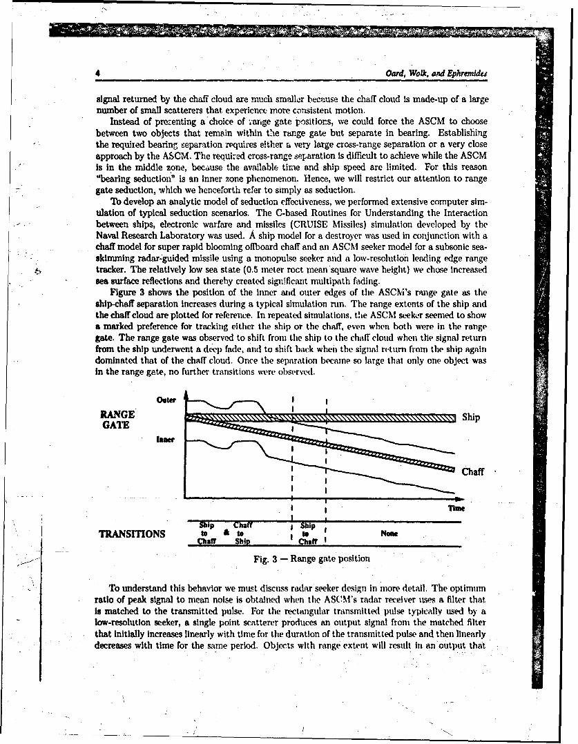
Figure 3 shows the position of the inner and outer edges of the ASCM's range gate as theship-chaff separation increases during a typical simulation run. The range extents of the ship andthe chaff cloud are plotted for reference. In repeated simulations, the ASCM seeker seemed to showa marked preference for tracking either the ship or the chaff, even when both were in the rangegate. The range gate was observed to shift from the ship to the chaff cloud when the signal returnfrom the ship undenvent a deep fade, and to shift back when the signal return from the ship againdominated that of the chaff cloud. Once the separation became so large that only one object wasin the range gate, no further transitions were observed.

Outer

RANGE ShipGATE

lIner

Chaff

T•me

Ship MIT . ShipTRANSITIONS to & to None

Chaff Ship Chaff I

Fig. 3 - Range gate position

To understand this behavior we must discuss radar seeker design in more detail. The optimumratio of peak signal to mean noise is obtained when the ASCM's radar receiver uses a filter thatis matched to the transmitted pulse. For the rectangular transmitted pulse typically used by alow-resolution seeker, a single point scatterer produces an output signal from the matched filterthat initially increases linearly with time for the duration of the transmitted pulse and then linearlydecreases with time for the same period. Objects with range extent will result In an output that

On 00 ifed SWulg of HadJ "d So)kl

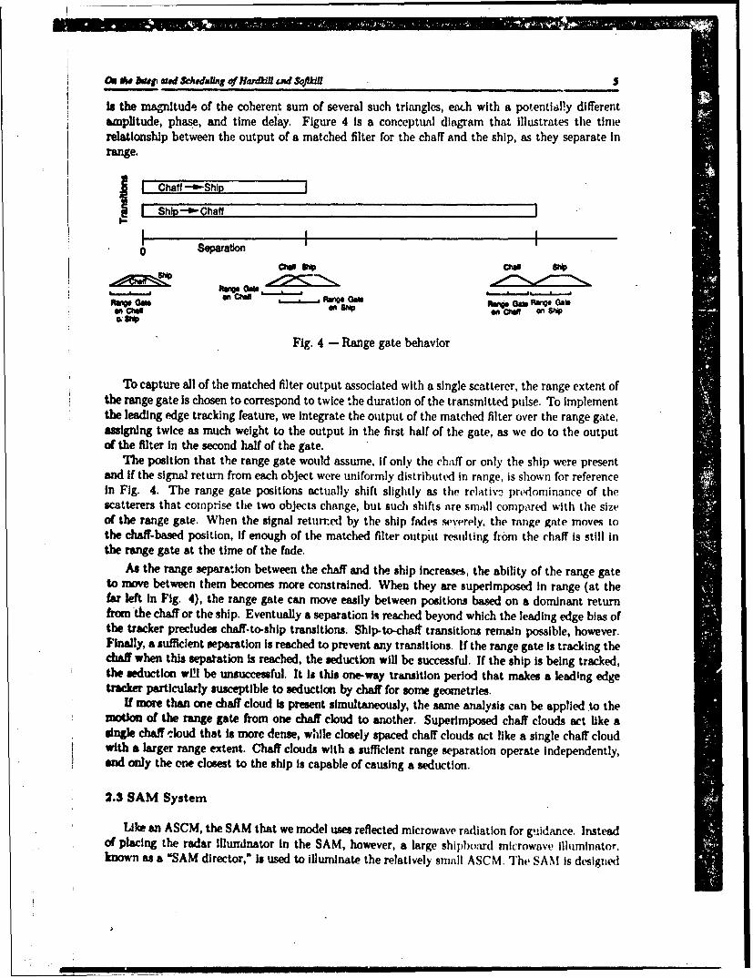
is the magnitude. of the coherent sum of several such triangles, eath with a potential!y differentamplitude, phase, and time delay. Figure 4 is a conceptual diagram that illustrates the timerelationship between the output of a matched filter for the chaff and the ship, as they separate Inrange.

-Chaff -0--Ship

I ShID -e Chaff

IsI0 ,Sewataon

Fig. 4 - Range gate behavior

To capture all of the matched filter output associated with a single scatterer, the range extent ofthe range gate is chosen to correspond to twice the duration of the transmitted pulse. To implementthe leading edge tracking feature, we integrate the output of the matched filter over the range gate,assigning twice as much weight to the output in the first half of the gate, as we do to the outputof the filter in the second half of the gate.

The position that the range gate would assume, if only the chaff or only the ship were presentand if the signal return from each object were uniformly distribut(d in range, is shown for referencein Fig. 4. The range gate positions actually shift slightly as the relativ? predominance of thescatterers that comprise the two objects change, but such shifts are smAll compared with the sizeof the range gate. When the signal returred by the ship fades vverely, the range gate moves tothe chaff-based position, if enough of the matched filter output resulting from the chaff is still inthe range gate at the time of the fade.

As the range separation between the chaff and the ship increases, the ability of the range gateto move between them becomes more constrained. When they are superimposed in range (at thefar left in Fig. 4), the range gate can move easily between positions based on a dominant returnfrom 'the chaff or the ship. Eventually a separation is reached beyond which the leading edge bias ofthe tracker precludes chaff-to-ship transitions. Ship.to-chaft transitions remain possible, however.Finally, a sufficient separation is reached to prevent any transitions. If the range gate Is tracking thechaff when this sepatation is reached, the seduction will be successful. If the ship is being tracked,the seduction wiLl be unsuccessful. It is this one-way transition period that makes a leading edgetracker particularly susceptible to seduction by chaff for some geometries.

If more than one chaff cloud is present simultaneously, the same analysis can be applied to themotion of the range gate from one chaff cloud to another. Superimposed chaff clouds act like asingle chaff cloud that Is more dense, while closely spaced chaff clouds act like a single chaff cloudwith a larger range extent. Chaff clouds with a sufficient range separation operate independently,and only the one closest to the ship Is capable of causing a seduction.

2.3 SAM System

Like an ASCM, the SAM that we model uses reflected microwave radiation for guidance. Insteadof placing the radar illundnator in the SAM, however, a large shipboard microwave illuminator.known as a "SAM director," is used to illuminate the relatively smiAl ASCM. The SAM is designed

6 Oard, Wolk, and EphremLdes

to fly a standard trajectory from launch until guidance infcrination is received. This trajectoryprevents the use of the SAM system in the inkier zone. Althtugh the minimum range at whichthe SAM system can be used is not necessarily the rane as the boundary between the Inner andmiddle zones we defined for ,he chaff, the difference i, sFght, arnd we consider them to be the samein order to avoid introducing additioi al notation.

The surveillance radar equipment installed on modern %% drships is able to detect an ASCM thatis above the horizon when tactical considerations allow its use. Against a sea-skimming ASCM,surveillance radar equipment has an i.itial de-.ection range of approximately 20 km. Midcourseguidance can be provided by a separate commF-nd channel or by homing on the reflected signalenergy from the SAM illuminator. Regardless of wlich technique is used for midcourse guidance,the ASCM must be illuminated for several second.- immediately before the SAM reaches it tofacilitate terminal guidance.

We have chosen to model a SAM system that uses reflected signal energy for midcourse guidance,because the requirement for continuous illumination increases the potential for harmful interferencefrom the SAM system. SAM director illumination is also limited by the horizon to about 20 kmagainst a sea-skimming ASCM. Because the ASCM must be illuminated for SAM guidance, it is notsensible to launch a SAM until the ASCM is detected. Once an ASCM is detected, however, a SAMcan be launched immediately. Because the SAM director and the SAM do not share a commontime base, a SAM using reflected signal energy for midcourse guidance has no way to determinethe distance to the ASCM. Therefore, each SAM guides towards all ASCMs in the middle zone onthe bearing illuminated by the SAM director. We assume here, for the sake of simplicity, that eachSAM tracks towards the closest ASCM.

Because SAMs employ a proximity fuse, the SAM is destroyed when it reaches the closest ASCM,regardless of the fate of the ASCM. The defender on the ship can rapidly determine whether anASCM has been destroyed by observing the reflected SAM director signal.

2.4 Chaff Effectiveness Model

The SAM system can significantly influence the probability of a successful seduction. Thisresults from domination of the signal returned from the chaff by the signal returned from the shipwhen the SAM director is oriented towards the ASCM. The effect depends on the relative strengthof the signal returns from the ship itself and from the chaff, the design of the SAM director antenna,and the design of the ASCM receiver.

Because we wish to study the effect of this interaction rather than its cause, we model theinteraction by introducing an overwhelmingly dominant point scatterer that is present only duringSAM director illumination. We have chosen a point scatterer with such a large radar cross sectionthat even -during the deepest fade it will dominate the signal return from the chaff.

Figure 5 shows the effect of Introducing the SAM director into our analysis of range gatebehavior. In that figure we have separately depicted the matched filter output associated with theSAM director by using dashed lines. As before, when the chaff and the ship are superimposed inrange, the range gate can move easily between positions based on a dominant return from the chaff,the ship, or the SAM director. Eventually separation A Is reached, beyond which the leading edgebias of the tracker precludes chaff-to-ship transitions when the SAM director is not illuminating the.ASCM. Ship-to-chaff transitions (and SAM director-to-chaff transitions) remain possible, however,and SAM director Illumination could still result in a chaff-to-SAM director transition. Subsequently,separation B is reached, at which the matched filter output from the SAM director signal is outsidethe range gate whenever the range gate's position is based on the chaff. Beyond separation Bchaff-to-SAM director transitions become impossible, although the leading-edge bias of the tracker

14 - ',4,

On. doa Ingrated S-Aeh fin of Ha~rdkdl anmd Sofikil 7

SrChaff -"Shlp

Chaff -"-SAM Director

I Ship -'--Chaff

I Ship'-'-SAM Director and SAM Directcr-b-Ship

SI I0 Separation A B C

.\, SAM P',SAMASMASM/ .pirecax . " (om 0'- IDkm/ 4 S aj,.hip A\P7 0.0~ /WS~'% Chaff '5Sho

i� � �om~e at'Flame Gatie Rage Gatel'-- o. RaS Ang Gate.n CSho iSR' on Chaff %"P0gO o wCaeafy n Ships itup 0' S?~iP

Fig. 5 - Range gate behvlor with a SAM director

still permits ship-to-chaff (and SAM director-to-chaff) transitions. Finally, separation C is reached.Separation C is sufficient to prevent any transitions except the slight change in position associatedwith a ship-to-SAM director transition or a SAM director-to-ship transition.

To achieve a successful seduction, the range gate must be tracking the chaff when this finalseparation Is reached. The probability of this occurrence depends on the signal returns from thechaff, the ship, and the SAM director during the seduction attempt. We describe in detail thecase in which the range gate Is initially tracking the ship in order to develop an expression for theprobability of a successful seduction, given that no previous seduction attempt was successful.

As Fig. 3 shows, at each instant in time the range gate is captured by the object within itthat is producing the strongest weighted output froni the matched filter. When the SANI directorIs not illuminating the ASCM, the ship's signi-l return usually dominates that of the chaff, evenwhen the chaff signal is weighted more heavily. Thus, when both objects are in the range gate, therange gate is normally tracking the ship. Occasional fiWles by the ship reverse this predominance.however, and lead to a temporary capture of the range gate by the chaff.

At relatively large separations, a range gate capture by the chlaffi plaVes mIost of tile ship outsidethe range gate. When this occurs, recapture of the range gate by the ship is precluded as long as theSAM director remains quiescent. If the range gate still includes the position of the SAM director,however, the extremely strong signal from the SAM director captures the range gate whenever theSAM director illuminates the ASCM'. Once the SAM director moves out of the range gate, SAMdirector illumination no longer affect•. the range gate's position. So, If the range gate is trackingthe chaff when the separation increases to the point where the SAM director is outside the rangegate, a successful seduction Is assured.

Reference to Fig. 5 allows us to construct a seduction model based on this behavior. We haveassumed that the range gate Is initially placed over the ship by the platform that launches theASCM. To ensure that the chaff cloud is initially in the range gate, w(e select launch parunretersthat ensure It to bloem at the same distance from the ASCM as the ship. As In the previous case,the range gate will then alternate between positions based on the ship and the chaff, usually in aposition based on the ship, until separation A in Fig. 5 is reached. SAM director illumination duringthis period simply serves to reduce the time spent tracking the chaff because during illuminationthe position of the range gate will be based on the SAM director signal.

Between separations A and B, SAM director illumination still results in capture of the rangegate by the SAM director. When the illumination terminates, the range gate shifts to the ship, anmdcapture of the range gate by 0he chaff becomes possible. Between separations B and C, capture of

8 Card, Wolk, and Ephmlardes

the range gate by the chaff remains possible, but the SAM director Is no longer able to recaptureit. In this region, if the range gate is tracking the ship, it moves blightly to track 'he SAM director.If, however, it is tracking the chaff, it remains on the chaff. So SAM director illumination duringthis period simply serves to lock the range gate in its present position.

Summarizing, if the chaff captures the range gate after the !ast SA.M director illuminationbetween separations A and B, a successful seduction is assured. The probability of such a captureby the chaff depends upon the pattern of ilhuminction between the time of that last illuminationand the time separation C is reached. A compleLe description of an illuninatioti pattern requiresspecifying whether the SAM director is illuminhting tlie ASCNI at each time step in this period.Fortunately, the minimum duration of a SAM flight. restricts the set of leasible illumination patternsto those that contain a small number of contiguous periods of illumination. The maximum numberof separate no illumination peiods depends on the length of the period between separations B andC, the minimum range of the SAM system, and the speed of the SAM.

Further simplification results from a time invariance that is a consequence of random fading.First consider the class of illumination patterns with a single no illumination period of fixed dura-tion. Since we can not readily control when the ASCM will observe a fade by the ship, we make ana priori estimate for the probability that a fade by the ship will occur during the no illuminationperiod that is sufficiently deep to cause a range gate transition. This probability estimate dependsupon a specific set of conditions that includes sea state, ship heading, and ship spvle. The fadesare a direct result of ship motion, which is a narrow band random process. For simplicity, weassume here that for any time chosen at random. the next fade is equally likely to occur at anytime within an interval roughly corresponding to a fundamental period of that narrowband process.Since we assume the phase of the fading patterns to be uniformly distributed, we hypothesize thatthe probability will be the same regardless of when A.he no illumination period begins. We call theduration of this single quiescent period D. At the beginning of the period the ASCM tracks theship, having just shifted there from the SAM director. As D increa;ses, the cumulative probabilityof a sufficiently deep fade by the ship increases as well.

Once separation C is reached, the outcome of the seduction attempt is completely determined.We define the time at which separation C is reached as our reference time tR and define the D(t)to be the unilluminated time that has been acciupilated by time t. The probability of seduction isthus a function of the duration of the no illumination period at the reference time

Ps: D(tR) ý- Pr{Successful seduction at time 11t; D(t). (1)

We could construct a similar function for more complex illumination patterns as well. Doing sowould improve the fidelity of our model by identifying the effect of temporal correlations within thepossible fading patterns. We believe, however, that we can bound the performance of the chaff withEq. (1). Because the probability is computed by averaging over every phase of every possible fadingpattern, the Ps function provides an tipper bound oni the seduction probability, when it is appliedto the total no Illumination time and a lower bound on the seduction probability when appliedto the duration of the longest no illumination period. Since either bound reflects the interactionbetween chaff and SAM employment and the argument for the upper bound Is easier to compute,we use the total no illumination time as the domain of Ps(.) instead of developing a more complexchaff effectiveness model.

The computation of D is then quite straig.htforward. If there Is SAM director illuminationbetween separations A and B, we begin counting D from zero at the end of the last such Illumination.When there is no such illumination, we :ftn begin counting D from zero when separation A isreached without significantly changing our analysis, because the ASCM is very likely to be trackingthe ship at that time. If there is SAM director illumination between separations B and C, we stopincrementing D when it begins and resume counting when it ends. - _

-4

ON A* nukegratud Scheduslj. of T•hakllt and Soflkiil 9

2.5 Measurement of Chaiff Effectiveness

If D(tR) = 0 the contlnvous illumination prevents a successful seduction (Ps = 0). To quantifythe remainder cf the dependence of Ps on D we simulated a series of texperimnents by using theCRUISE Missiles testbed. Figure G shows the geometry we used. This geometry results inl sufficientrange and cross-range separation between the chafr and(I the, ship) to allow a seduet ion. iid it exploitsthe leading edge bias of the tracker by assigning tile Ship a velocity coililpollvtll iwily fr',ll: tII!

ASCM. No wind or current was applied, and unaccelerated ship motion was assumed. Because themaximum range of the SAM system again-+, low altitude ASCMs depends on the elevation of theSAM director, the SAM director is normally placed high on the superstructure near the middleof the ship. For this reason we placed the SAM director 35 m directly above the ship's ccnter ofgravity.

20 km

300n/s

StationaryChaff

Fig. 6 - Monte Carlo simulation Initial conditions

The ordinate of the graph in Fig. 7 shows the empirical probability of seduction that resultedfrom continuous illumination from the beginning of the run until the separation plotted on theabscissa was reached and then no furthe; .lumination until the ASCNI reached the in,,r zon,. Themeasure of separation that we have chosen is the range separation between the ship's (',enter ofgravity and the geometric center (,f the chaff along the ASCM-to-chaff line of sight. We calculatedthis empir-,-d probability by conducting a set of simulation runs and observing whether the ASCMwas tracking the ship or the chaff at thi end oe each run. In each trial we independently selecteda pseudorandom seed for the ship and sea motion components of the model. This results in trialoutcomes that are independert and identically distributed. Under this condition, the empiricalprobability approaches the parameter of the underlying binomial distribution as the number ofruns increases. A sufficient number of runs were conducted to achieve a 0.9 confidence that thetrue seduction probability lies within a ±0.1 confidence interval of the plotted value. Data pointsare plotted at approximately 25 m Intervals.

Examination of Fig. 7 reveals that continuous illumination past 375 in of raiige separat.onalways prevents a successful seduction. Therefore, 375 m In this geometry corresponds to separationC In Fig. 5. The time without illumination (D) before separation C is reached is plotted on thetop of the graph. The data show a nearly linear Increase in seduction probability with an increaseIn D. The limiting probability of seduction (In this case 1.0) depends on the relation between thesignal from the chaff and the signal from of the ship at the deepest point of a fade by the ship forthis geometry. We call this limiting value P,,•.. The time without lllumnination that is required toachieve this limiting seduction probability depends on the frequency with which fades occur, whichIs determined by the ship motion and the sea moLion In the simulation. NV. call the smalkst valueof D(tR) that maximizes the probability of a successful seduction D,,,,,.

10Oerd, Wolk, pndEphremide

Time WI•iu Iqlvnkn (sowrur)S 611 4 20G

0.4.

031X 350 400Sepgofi a n Tem•ation (metors)

Fig. 7 -- Typical s duction probability function

Separation B in Fig. 5 can be found by determining the position of the range ate when it istracking the chaff and then by computing the minimum range separation necessary to place all theenergy from the SAM director cutside of the range gate. In our low-resolution ASCM seeker weuse a 2 jAs range gate because we have a 1 us pulse width and a matched filter. When the leadingedge tracker is tracking the chaff, the trailing edge of the range gate is located approximately 0.63ps beyond the geometric center of the chaff cloud in signal space. The geometric center of the chaffcloud in signal space corresponds to the center of the chaff's flat spot in Fig. 5. When coupled withthe 1 ps matched filter, a 1.63 ps round-trip tansit time difference between the geometric centerof the chaff and the location of the SAM director (the peak of ,he SAM director signal in Fig.5) Is sufficient to prevent the signal returned by the SAM director from influencing the tracker'sbehavior. For simplicity we have placed the SAM director directly over the ship's center of gravity.Thus, separation B is 245 m for this geometry. Note that we have implicitly assumed that thebias in the range gate is sufficient to prevent the signals reflected by closer parts of the ship fromsignificantly affecting the leading edge tracker's behavior in this case.

Determination of separation A in Fig. 5 requires an additional experiment. We began by cre-ating a single no illumination period of duration D, 1 . that ends when separation C is reached.We then shifted the no illumination period earlier in time while maintaining a duration of D...until the period barely lasted past separation B. If a reduction in seduction probability had beennoted, the smallest separation that avoids the reduction would be separation A. However, no suchreduction occurred. From this we conclude that separation A is less than 155 m (the smallest sepa-ration attempted) for this geometry. In that case the precise value of separation A is insignificant,because a lack of illumination between the actual value of separation A and separation B wouldhave the same effect as a lack of illumination between a separation of 155 ni anq separation B.Therefore., we can consider separation A to be 155 m. Although this choice could rdsult in a failureto count D between the actual value of separation A and a separation of 155 ni, the resultingseduction probability would be unaffected because either the seduction probability would alreadybe maximized or an intervening illumination would reset D.

We found similar seduction probability functions for other initial geometries as well. Variationsin ship velocity produced the expected compression or expansion of the time axis. Slight shiftsIn separations A and C were also observed. I This occurs because the tracker is -affected by therange extent of the ship along the ASCM-to-ship line of sight, which varies with the ship's heading.Some ship headings also result in larger or smaller signal returns from the ship, which changes the

On. the haigrawed Sckhdulhug of Hardkili and Sojttil 11

effectiveness of the chaff. When present, this effect results in compression or expansion aloag theseduction probability axis. The value of P,,, is easily found by conducting a sirgle set of runswith no illumination. ChangIng the initial position of the chaff cloud slightly did not affect theoutcome of our experiments. In particular, initial range separations between 0 and 270 in resultedIn truncated versions of Fig. 7, and similar initial cross-range separations had no significant effect.Varying the position of the ASCM In the middle zone had no significant effect, because the periodbetween multipath fades Is nearly constant, while the ASCM is in the middle zone.

2.6 SAM System Effectiveness Model

The position of the chaff cloud can influence the performance of the SAM system. If the chaffcloud is placed directly between the ship and the ASCM at a low altitude (near the end of its life),it could prevent the SAM direct illumination from reaching the ASCM. This would result in lossof SAM guidance anu require destruction of the SAM before it reaches the ASCM. This situationcan be avoided by choosing a chaff bloom position that places it astern of the ship-to-ASCM lineof sight before Its altitude decays enough to cause a problem. Since that tactic is compatiblewith the requirements for optimal chaff effectiveness, we shall adopt it and consider SAM systemeffectiveness In isolation.

Because our focus Is on the SAM/chaff interaction, we have chosen the simplest possible modelfor SAM system effectiveness. We model the effect of a SAM, intercept with a constant PK thatrepresents the probability that a SAM intercepting an ASCM in the middle zone will destroy it.The parameter PK can be chosen based on simulation results or operational experience. If anASCM is intercepted but not destroyed, It can later be Intercepted again by another SAM. Bychoosing PK to be constant, we are treating each intercept as an independent event.

3 ENGAGEMENT MODEL

Although the individual effectiveness models are adequate to determine the distribution on theoutcome of a single event, the integration of these into a unified whole remains to be done. We areInterested in the effectiveness of several applications of the SAM and chaff systems in defendingagainst an attack by multiple ASCMs. We restrict our analysis to the case in which all the ASCMsarrive from the same direction, and each travels with approximately the same velocity, because bydoing so we simplify the engagement model while preserving the interaction we wish to study. Wechose the arrival angle shown In Fig. 6, because it accommodates the requirements of our tactics.Since Fig. 7 indicates that the seduction probability is closely approximated by a negative-goingramp function, we have used that approximation to construct an idealized Ps function defined as

PS = P " D,,. - min{D, D,,(}DS•m (2)

Inspection of Fig. 7 suggests that a reasonable value for D,,.. is 8. The interaction we wishto study is only present when P,,. assumes a moderate value. If high assurance of a successfulseduction were possible, SAM employment Is not necessary. On the other hand, a low value forA,. keeps seduction from being worth considering, Thus, the interaction we wish to study is onlysignificant when P,,,_ assumes a moderate value. For this reason we have chosen to assign P,,, avalue of 0.5. Similar considerations dictate the choice of a moderate value for Pj. Therefore. wehave somewhat arbitrarily assigned PK = 0.3.

In developing a model for this multiple ASCM problem. which we will call the "engagementmodel," we must examine the effect that a single application of each defensive system hms ondifferent ASCMs. Because it is extremely unlikely that two ASCMs would be so close to each other

= 7- 7!

-r.,-°-

12 • Oard, Wolk, and Ephremides

that bc,th could be destroyed by the same SAM, we will ignore that case. Hence, each SAM canaffect st most one ASCM. A single chaff cloud could, however, affect every ASOM in the middlezone. Lach ASCM arriving from a given direction will observe the same range separation betweenthe chaff and the ship at the same time. Since we have restricted o•u•r atteiltion to the case in whichall ASCMs arrive from the same direction, every ASCM in the middle :one will experience eachseduction attempt simultaneously.

The fading on which seduction depends is caused byv imultipath propagation and by changesin the ship's orientation. Multipath fading occurs when the length of two raypaths differ by ahalf-wavelength (modulo the wavelength). The dominant multipath interference occurs betweenthe direct raypath and the raypath reflected once off the sea surface. ASCMs with the same pathlength difference (modulo the wavelength) will observe synchronized fading, while for other A.SCMsthe observed multipath fades will occur at different times. Fading due to changes in the ship'sorientation occurs When many of the normally dominant scatterers are viewed from an orientationin which their reflectivity is low. All ASCMs arriving from the same direction should observe

synchronized orientation-based fading. Although it should be possible to construct an accuratemodel of the relationship between the fading observed by multiple ASCMs, we have chosen to treatsimultaneous seduction attempts as mutually independent events. This choice allows us to specifystate variable transition probabilities individually rather than in all possible combinations, therebyreducing the complexity of the model

The high speed of each ASCM and the limited number of ASCMs that an adversary couldreasonably use naturally leads to a finite time horizon formulation. To facilitate computationalsolution, we have chosen a discrete time specification for our engagement model. To simplifythe formal specification of the model we will assume that all moving objects travel at a constantvelocity. This assumption allows us to express distances as time periods, eliminating unnecessaryunit conversions.

3.1 States and Controls

Table 1 shows the state variables for the engagement model. We use the index i to distinguishbetween similar state variables that refer to different ASCMs and allow i to range from 1 to 7n,where m represents the maximum number of ASCMs that may arrive. Each state variable isdiscussed in detail below. We refer to the entire collection of state variables at time t as the "state"at time t, Xt. Note that while we use a subscript i on a state variable to indicate the associatedASCM, we use the subscript t on the state (and later on the control function) to represent time.We have included enough information in the state to construct a controlled one-step iiarkoyvmodel,which is required for one of the optimization techniques that we will consider.

Table 1: State variables

Ai Time until ASCM i reaches the ship (s)C Time until chaff enters seduction region (s)D Time since SAM director status change (s)N Number of remaining SAMsS Time until SAM intercepts closest ASCM (s)Ti Whether ASCM i is tracking the ship (True or False)

On 1w huag.-aed Scheduling of Hardkinl and Sofdkill 13

We sample state transitiois once each A seconds, with the first transition beginning at time0 and the last at time r - A. Because the next state may depend on the outcome of one ormore random events (ASCM detection, SAM intercept, or seduction attempt), the transition fromthe present state to the next state will, in general, be stochastic. Figure 8 specifies the allowedtransitions for each state variable. Each arc is labeled with the condition under which that arcmay be taken. When the transition is not deterministic, the probability the transition occurs isseparated from the condition by a comma.

C, C-0

N* OtherwiseNo

OtL,, C Truee.

Otherwise O e

o~. (C >CA)v ((cncC A C)^(S • )) z=i

OthewiOec(DY (C<CO^(S<O) "

k 4> C, £-PA(n~t)

i•S O)^(i =minT*0 <AJ $ €4 I),PK c)Otherwise

TI: otherwise 0 A (C"O),P CD) Fl Always

Fig. 8 - State variable transition diagrams

We will restrict our attention to ASCM arrival distributions that depend only on time andthe number of ASCMs that have already been detected. We will use the information about thenumber of previously detected ASCMs to limit the attarker to m ASCMs. This is a relativelysimple formulation that reflects both the attacker's lack of detailed knowledge of the defender'sstate and the defender's uncertainty about the attacker's strategy while producing a controlledone-step markov model. Therefore, we take as given:

PA (n, t, a)

= Pr(n ASCMs will arrive at time t given that a ASCMs have already arrived). (3)

Because a relatively large range separation Is required between chaff clouds if separate seductionattempts are to occur, relatively few seduction opportumities can be cre'ted for each ASCM. Wehave chosen to repeatedly fire chaff rounds at the minimum effective interval to maximize thechance of a successful seduction. This decision reduces the complexity of the control policy we seekwithout eliminating our ability to observe the effects of the SAM/chaff interaction.

Accordingly, the ship has available one control L(t). Setting L(t) to True represents the launchof a SAM at time t. Setting L(t) to False represents foregoing the opportunity for a launch at

14 Oard, Wolk, and Ephr nides

that time. L(t) is constrained to be False if a SAM is already in flight or if the SAM Inventory"Is ehae.usted. We make it possible to enforce an inventory constraint by defining N to be thenumber of SAMs remaining. Initially we set N to No, the number of SAMs that. are available atthe beginning of the engagement.

The peiiodic nature of chaff deployment is represented by a counter C that represents the timeuntil the next chaff cloud will next be properly positioned for a seduction attempt. C initially hasa value Co, which represents the phase of the periodic chaff replacement. Subsequently, C countsdown modulo C,., + A.

We use Ai to represent time remaining before ASCM i reaches the inner zone. .4 is initiallyset to oo, which represents a remaining time greater than rM. As long as ASCM i is outside themiddle zone there is a chance that it will arrive at the outer boundary of that zone and be detected.There will be n arrivals at time t with probability PA (n, t). By convention we assume that ASCMsare numbered in the order. of their arrival. Therefore, ASCM i arrives at time t if there are morearrivals at time t than there are lower numbered ASCMs that have not yet arrived. When ASCMi is detected, Ai is set to TrM. Ai subsequently decrements until ASCM i reaches the inner zone oris destroyed by a SAM intercept. For ASCMs, which reach the inner zone, we allow the value ofAi to continue to decrement below zero and interpret negative values of Ai to represent ASCMsthat are no longer in the middle zone. If ASCM i is the closest, ASCNI in the middle zone (i.e., i isthe smallest j for which 0 < Aj < rTM) and it is destroyed by a SAM intercept, we set Ai to -oo,representing an ASCM that will never reach the inner zone (and thus never hit the ship).

Intercepts occur when the most recently launched SAM reaches the closest ASCM in the middlezone. We assume the SAM and ASCM both move with constant velocity and define Vs to be theratio of the velocity of the SAM to the velocity of the ASCM. The distance between the SAMand the ASCM will decrement at Vs + 1 times the rate at which Ai is decrenmenting. At time t,min{Ai(t) : 0 < Ai(t) rlM) + rTj more seconds would be required for the closest ASCM in themiddle zone to reach the ship. If we divide these two quantities and adjust the result to be aninteger multiple of A, then at the time the SAM is launched we can calculate the time at whichthe intercept will occur t1 as

tm(t) = t [ind )} + A' -J.A (4)tdt) =t + i Vs + I

The state variable S is used to carry this information forward from the SAM launch time to thetime of the intercept. Initially S is set to -oo, where we interpret negative values of S to representa state with no airborne SAM. When a SAM is launched, S is reset to the calculated intercept timeti. Subsequently, S decrements to zero, at which time an intercept is recognized. Since at mostone SAM can be in flight at a time, a scalar value suffices to represent this information.

The illumination duration D remains zero until separation A is reached, which occurs whenC = CA. Subsequently, D is incremented by A whenever there is no airborne SAM and reset tozero when there Is an airborne SAM. Once C reaches separation B, which occurs when C = CB, Dcontinues to increment when there is no airborne SAM but holds its value when a SAM is airborne.

The Boolean state variable Tj whether ASCM i is tracking the ship. Initially Tj is True Vibecause all newly detected ASCMs are assumed to be tracking the ship. Seduction attempts occurwhen C = 0, and they can be effective against any ASCM in the middle zone (i.e., any ASCM i forwhich 0 < Ai < TM). At each seduction attempt Ti will become False if the seduction attempt issuccessful.

We have collected all of the parameters of the engagement model in Table 2 and indicatedtypical values for a simple instance of the model. While these parameters are often somewhatarbitrary, the entire set of parameters must be chosen in a consistent manner. For instance, rAmust be some multiple of A so that it will be possible for Ai to reach zero.

On As hnegrared Sheduling of HaMWU and Soft W IS

Table 2: Engagement Model Parameters

Parameter Value Units DescriptionA I seconds Time quantumI" 147 seconds Final timeI'M 48 seconds ASCM flight time in the middle zone1 12 seconds ASCM flight time in the inner zoneCo 30 seconds Time of first seduction attemptCA 15 seconds Value of C for separation ACD 8 seconds Value of C for separation BC. 19 seconds Maximum time until the next seduction attemptD~w. 8 seconds Ma::Imum no-illumination durationm 3 ASCMs Maximum number of ASCMs which may arriveNO 5 SAMs Initial SAM inventoryPK 0.3 Probability that a SAM will kill an ASCMPM= 0.5 Maximum seduction probabilityVs 3 ASCM Speed Relative speed of a SAM

3.2 Observations

The vndue of most of the state variables can be observed or deduced without error at eah time.Figure 8 identifies the inilal value for each state variable using a small arrow. Since C has a knownInitial value and it evolves deterministically, C(t) is known a priori for all 1, regardless of the policyselected. The evolution of N is completely determined by the control L(t). which becomes knownas it i5 chosen at each time. So N(t) becomes known by time t.

Although Ai evolves stochastically, its value can be observedx at each time. Because the velocityof an ASCM is nearly constant, Ai is directly proportional to the d;stance botween the ASCNI andthe ship. Thus, Ai (t) can be observed at time t without significant error by using surveillanceradar equipment. Since (Ai (t)}) is known in this way at time t and L(t) is also known at time t,S(t) can be calculated by using Eq. (4) at time t. And finally, once S(t) and C(t) are known, D(t)can be calculated.

As long as no seduction has been attempted against ASCN1 i, T, evolves deterministically andits value can be computed. Once a stochastic state transition occurs, however, this is no longerpossible. Furthermore, it is Impractical to observe Ti while ASCM i is in the middle z7one. T7(t)again becomes known with certainty only after ASCM i enters the inner zone and reaches eitherthe ship or the chaff cloud.

We will refer to the known state variables at time t as the observation at time t, Oj and definea function 0 : Xt " OQ. Ot consists of every state variable in Xt except Ti(t) for those ASCMsthat were in the middle zone during a prior seduction attempt and have not yet reached either theship or the chaff.

3.3 Reward Function

We assume that a single hit by an ASCM is sufficient to disable the ship for the remainder ofthe engagement. For small ships such as frigates and destroyers this is a reasonable assumption.Therefore, we wish to find a policy that will maximize the probability that no ASCMs will hit theship between time 0 and time r.

• 16 Oard. Wolk, and Ephrermides

By a policy we mearn a set of functions indexed by time, the range of each being the control tobe applied at that time. In general. we would like to base our cont ml d1cision'. oil all of the lisoefu

- information available at each time. If we were to choose X, as Ithe donman for the control filtictioiat time t we would obtain a one-step markov model. l.'irthermorv. since X, captures all of therelevant inforniation about prior states and controls that is ne(cessary to determine the next state,adding prior state and control informiation to the domain of the control function would not changethe optimal value of the reward function. Unfortunately, it is sometimes impossible to observe partof Xt. When part of Xj cannot be observed, a control fumction that requires all of Xt as its domainwould not be useful to a defender.

Another obvious choice for the domain of the control function at time t is 0,, the observationat time 1. Since 0, C X1, this choice would yield a otie-step markov model using a control functionthat could be used directly by the defender. in this case, however, adding prior observations to thedomain of the control function could potentially improve the optinmal value of the reward function.In addition, our knowledge of system dynamnies also makes it useful to inclde the prior controlswe have applied in the domain of the control function. "To quantify this dependence we define theinformation vector at time t to be

Jo = o0I = {Oo,...,OL(O),...,t(t-A)), (i E ( , -

The policy we seek is a set of functions r Ili, It ý- L(t))}-A. We wish to find the policy irthat maximizes the probability that the ship is not hit when that policy Is employed. Therefore,we choose as our reward function

J, =- Pr{Ship not hit: ir)

In this notation we have explicitly identifild bot h the event (Q Ship trot hit }) and the parameter(7r) that determines the probability of that event. We shall use this notation extensively to callattention to the functional dependence of a distribution on certain parameters.

4 OPTIMAL SCHEDULING TECHNIQUES

We seek to find an optimal policy ir* for which

J,'. max= h).

We shall present two techniques for finding an optimal policy, exhaustive search and dynamicprogramming.

4.1 Exhaustive Search

Exhaustive search is a brute-force strategy that can be efficient when the number of alternativesthat must be considered is small. In the exhaustive search strategy we first compute the value ofJ, for every possible policy ir and then choose the policy that maximizes that value. We begin bydeveloping an algorithm for computing J,. Starting with the definition of the reward function weapply the law of total probability:

J, = Pr{Ship not hit; 7r)

= I - Pr(Shtp hit;ti}

= 1- • Pr{ShiphitlXo,....,Xr;irl.Pr(Xo,...,Xr;,r} (5){Xo,...,Xr}

*AOWhg kriwed Scwadainum Md'w"i "d S~flkil 17/ I

Tie engagement model described in Fig. 8 specifies Pr(Xt+AIXt, L(t)) and specifies a delta,'/function for Pr{Xo}. Since L(t) = 1(), we can ,tse the cne-step markov structure of the modelto compute the second probability in Eq. (5):

Pr{Xo,...,Xr;ir) = Pr(Xo} IJ Pr{X,+AjX,.ji,(I,)}. (6)t=0

Computation of the first probability in Eq. (5) Is somewhat more complex. In our analysisabove we determined that the ship will be hit if and only if at least one ASCM reaches the innerzone without being seduced. That occurs if and only if there exist an ASCM i and time t for whichboth A, (t) = 0 (i.e., at time t ASCM i reaches the inner zone) and T. (t) = True (i.e., at time tASCM i is tracking the ship). This formulation captures the effect of a successful seduction directlyby using T, but relies on A, to keep ASCMs that are destroyed by SAMs from being considered.Using the indicator function liE•,*J that has value 1 when the event occurs and 0 when it doesnot

Pr(Shlp hitXO, .... ,X r ;,r) = li3(iC)(A,(t)=O)i(T,(t)V' ,.e)) (7)

Combining Eqs. (5), (6), and (7) and then eliminating zero terms from the summation we get

•I I = 1- 1 3{0(iA. A(A)=O)A(T, (t)='True))" Pr{Xo) . j Pr{Xt+aIXt,pt(Iz))(Xo,...,x 7.})=

T-A

= 1- Pr(Xo). [1 Pr{X,+aIXt,p,(J,)). (8){Xo,....x.r }93(,t)(A, (t) =O)^(T, (I)=7ýu) 8=0

Since we can repeatedly apply the definitions of pi, I1, and ) to find pi(lh), given {Xo. Xt},this equation provides a somewhat cumbersome way to compute .1, for any policy ir. By tryingevery policy, we will eventually find the one that maximizes J,. Examination of Eq. (8) reveals thatthis computation will be most efficient when the time horizon is short and the number of possiblestate sequences Is small. Since the computation is repeated for every policy 7r, practical applicationof this technique Is only possible when there are few times when more than one alternative Isavailable.

4.2 Incremental Computation of the Reward Function

The exhaustive search technique requires that every possible path through the state space beconsidered. Multiple control alternatives or stochastic state transitions will result In exponen-tial growth in the number of paths. If we define computational complexity to be the greater ofthe asymptotic time or space requirements of an algorithm, the computational complexity of theexhaustive search technique grows exponentially as the number of time steps Is Increased.. The controlled one-step markov structure of the engagement model suggests that it may be

useful to view this optimization problem as a multistage decision process and consider incrementalcomputation of J,.. Incremental computation can result In greater efficiency by computing Inter-mediate values for each unique subpath only once. Two approaches to Incremental computationare possible.

Incremental computation forward In time Is done by walking a decision tree to find the optimalpolicy and considering several branches at each step in which a stochastic state transition occurs.Only reachable states are considered when walking a decision tree. As the number of reachable

//

/

18 Oard, Wolk, mad Ephrwrdes

"states becomes large, however, a tree walk will consider malay of these states more than once. Thisrequires either repeating the computation each time a state is considered or storing the previousresult. If recomputation is chosem,, the computational complexity of a tree walk grows exponentiallyas the number of time steps is increased. When intermediate results are stored, a large inte'ne-diate storage area that grows as the number of time steps Is IncrevL'ed will be rnxuired; however.computational complexity will grow linearly with the number of time steps.

"Incremental computation backward In time is done by constructing a state lattice bcckwardfrom each possible final state. The algorithm for incremental computation backward in time isknown as dynamic programming. Because every state is considered only once at each time, thecomputational complexity of a dynamic programming solution grows linearly as the number of timesteps Is Increased. Although dynamic programming nreuires internediate storage for one value foreach state, the required storage area does not change ats the number of time steps is increased. Forthat reason, we will next apply the dynamic programming algorithmi to this )roblem.

4.3 Dynamic Programming

\ In dynamic programming we seek to reduce the problem of seleting the optimal policy to asequential selection of optimal control functions for each time. The dynamic programming algorithmworks by associating with every state at time t a value that represents the expected reward thatwould be earned if we started in that state at time t and employed an optimal policy between timet and time r. This set of optimum expected rewards can then be used to compute the optimumexpected reward associated with any state at time t - A, if the incremental effect of each possiblecontrol that could be applied from that state at time t - A is known.

Conventional dynamic programming is valid for a reward function fortned as the expectation ofa sum of partial rewards. Appendix A describes a similar algoritlhn for a reward function that isthe expectation of a product of partial rewards. Appendix A identifies live properties that a modelmust possess before that dynamic programming algorithnm call be applied:

(a) A finite set of states

(b) A control function with the state as its domain

(c) A controlled one-step markov model in which the distribution on the next state is determinedby the )resent state and the present control.

(d) A set of nonnegative partial rewards functions, each of which has the state at one time as itsdomain.

"(e) A reward function that is the expectation over the state sequence of a product over time ofthose partial rewards.

4.8.1 Computation of the Reward FUnction Using the Information Vector

Because we do not have perfect knowledge of the state at each time, we must use the informationt vector It as the domain of control function at time t. To satisfy property (b) we must treat It as

If it were a state in our development of a dynamic programming solution. That choice satisfiesproperty (a) because It is a finite union of finite sets.

Property (c) then requires that lt+a be a known stochastic function (called the next statefunction) of It and pt(It). We will show the existence of a next state function for It by brieflysketching its derivation. We begin by applying the definition of It to the next state functionfrom property (c) in Appendix A and then simplify the resulting expression, thuis observing that

On iW ksM'ated ScAafuflig of HaidiW aiw' SofitW 19

Lt) = j,,(It)Pr{It+Alt; pd(t)}

= Pr[Oo,..., . O,+,, L(O),..., L(t - A), L(t)10o,.. 0O, L(O). LI - A); p,(I,))= Pr(O,+AIO°"",Og L(O)," L(t - A); L(t))" (9)

Now recall that each Xt+a Is associated with exactly or.e O+,%. So 0 partitions the statespace. We em therefore express the value in Eq. (9) as a sum ot probabilities, then apply the law oftotal probability and simplify the result by using the one-step iarkov property of the engagementmodel:

Pr{Ja+A11t; dtU)}

= , Pr(Xa+AIOo,... 0Oj, L(O),... L(t - A); L(t))= E 3O+ = O( X+A)

Xt+A9O,+A =O(X,+ ) aXo..., (Oo..O,}O(IX....XJ)

Pr{Xt+& Xo,..., A ..O, 0 O, , 0,, L(O) .... L A(t) )SPr{Xo, . .[ Xii~o,....,Or, L(O),.. . ,L( t -A); £(t)}

X,+a63O,+,=0o(X+, 1,) {Xo..Xg)(Oo....ou}=O((Xo.....X, 1 )

"Pr(Xt+&jXg; L(t)) . Pr{Xo,..., XIOo..... O, L(O)..... L(t - A): L(t))

(Xo,....X, + , O• ..,O,+a=o({Xo ...... V I)Pr(Xt+AIX,; L(t)) Pr{Xo, ..... X,O.... O, L(0),.... L( - A); L(t)}. (10)

The first probability in Eq. (10) is specified in Fig. 8 ajid the second can he found by firstapplying Bayes' theorem, then simplifying the res;ult thlrotghi the observation that in Eq. (10){10,. .,Or) = 0((Xo, ... ,Xr)), and finally by using the markov property to write the jointprobability as a product of conditional probabilities

Pr{Xo,. .. , XjOo,..., Og; 7r)Pr(Xo,..., Xg; r)}. Pr{Oo,..., OtIXo ....- , Xt; r}

{Xo....X3Oo....o)=O((Xo,...,X,)) Pr{Xo, ... Xt; r) - Pr{Oo, ... . OXo .. .. -Xt; 7r

= t Pr(Xo,....,Xt;ir)

.. , o,,=o(Xo.. Pr{Xo,..., Xt; 7r}Pr{Xo}.- l'I7='o' Pr{Xt,+AjXt'; L(t')}

E{Xo,....X,{OOX..,x)) Pr{Xo) }lni- Pr(Xe+4 1XI'; L(t').)

So the next state function is well defined and property (c) is satisfied. Properties (d) and (e)require that the reward function be formed as the expectation over the state sequence of a productover time of nonnegative functions of the state. To put our reward function in this form, we startwith the definition of the reward function and again apply the law of total probability followed bythe definition of expectation to obtain:

Jw = Pr(ShIp not hit;,7r)

= I-Pr(Ship hit;x)

= 1 - Pr{Oo,...,Or; r) . Pr{Ship hit!Oo...Or: ir)(Oo....,OT)

1- E jPr(Ship hitlao..... Or; tnir, 1. (01)tfOo.....or)

20 Oard, Wolk, and Ephremidea

In our notation for expectation, we place the parameter on which the distribution dependsinside the brackets after a semicolon. Now we can derive an analytic expression for the probabilitythat the ship is hit by recalling the condition we introduced earlier

Pr{ShIp hitiOo,. .. ,Or; r) Pr(3(i, t)(Aj(t) = 0) A (T'(t) - Thue)IOo-..0r; 7r)

-= 1 - Pr(V((i, t) B AM(t) = 0)(Ti(t) = False)IOo ... O., ; ir

S1- fi Pr(Tj(t) = FaIsefOo,...,Or;7r)

"The last step is based on the mutual independence of T1(t)Vi at every time t, given the samecontrol sequence. This independence Is a consequence of the known value of T1 (0) and the (assumed)mutual independence of simultaneous seduction attempts. Substituting our result into Eq. (11) weget

I = 1- E 11 - i Pr(Ti(t) =FalseOo,...,Or;7r);,r], ~(a,t)3Adt)=O

.1 = E I nl Pr(Ti(t) - FalselOu .....-Or;7r}:ir. (12){oo,...,orl}(,•,t=

Since T, (t) is not known, we must compute its distribution based on the available information.

Pr{7(t) = FalseIOo,., Or; 7r)

= 1 - Pr{Ti(t) = TruefOo,... ,Or; Ir= 1 -Pr{No successful seduction attempt against ASCM i by time tjOo,.... r; ir}.

The relevant seduction attempts for each ASCM are those that occur while it is in the middlezone. From the state transition diagram for T, in Fig. 8, we see that wvhLction attempts onlyoccur when 0 < Ai < Trh, and C = 0. Using this observation, the markov structure of Ti, and thedefinition of PS we proceed as follows

Pr{(T(t) = FalsefOo,..., O.r;,r1 - Pr{V(t' < t)((C(t) = O) A (0 < Ai(t') < 1sr))

* (Failed to seduce ASCM i at t')IOo,.. ,Or;i})1: I- [ Pr((Falled to seduce ASCM i at t')jOo, ... OrT ir)

- 1- fi (1 - Pr((Seduced ASCM i at t')10 0,..., Or; ir))

= 1 - [3 (I - Ps(D(t'))). (13)

Combining Eqs. (12) and (13) ari then separating the outer product into products over t andi we get:

= E 0 -i (1- f (I-Ps(D(t'))));7r)100,...,Or} (i,8)9Aj()=o (e:_<O9(¢{V)=O)^(O_<A,(t1)5<•A)

= E I11 II (1- H l- Ps(D(t'))));ir. (14)O r) t=O isA,(t)-O (I'<t)D(C(t')=O)A(O<_A,(t')<:,M)

We now observe that the policy 7r establishes a one-to-one correspondence between the sequenceof observations {O0,... ,Or) and the sequence of information vectors {Io .... t Ir). Therefore, wecan rewrite Eq. (14) to get an expression in the form required to apply dynamic programming:

On Aw hivsrared Scheduft'g of Hardkli and Sofikil 21

7"

, 10 E .7) f (1 J (1 -Ps(D(t',))); 7r]o ..J t •- 0 i9A M()= O (t':5 t)9(C (t')=O)A(Of5A ,(t') <_•#t)

- E IlI g,(h) (15)to... JT} t=o

where we define,

gt(it) = R (1 - J (1 - Ps(D(t')))) V E (0,.. r}. (16)i3•Aj(t)=O (t'-<t)9)(C(t')=O)A(O<-A.(t'):_rM)

The form of Eq. (15) satisfies property (e). Equation (16) satisfies property (d) because 9t(h)can be computed without reference to states for times later than t. In particular, gt(It) can becomputed solely by reference to C(t'), Ai(t'), and D(t') for t' 5 t. Furthermore, gt(I) is nonnegativebecause it is the probability that every ASCM leaving the middle zone at time t has been seduced,and probabilities lie in the Interval 10, 1]. We have therefore demnonstrated all five of the propertiesrequired to apply the dynamic programming algorithm in Appendix A. As a result we can compute.1,. ~8,,

Vr(Ir) = gr(I7) (17)

Vt(It) = max{ E IVt+A(h+1 ) gt(It);Ilt(lh)] (I E (0 ..... r - A)) (18)pdlt) (It+A1I

J'. = E IVo(Io)]

4.3.t Constraining State Space Growth

As t increases, the cardinality of h grows rapidly. This means that the maximization In the dy-namic programming algorithm must be performed over functions with rapidly expanding domains.However, very little of the Information In h is actually used each time to compute the rewardfunction. Using this insight, we will construct a related optimization problem with a state of fixedcardinality that can be used to find the optimal policy for our original problem.

Examination of Eq. (16) reveals that the partial reward at time t depends on the value of Dfor every time an ASCM leaving the inner zone at time t might have been seduced. By includingthis Information in our new state, we can construct a one-step markov model without recourse toan Information vector. Equation (13) can be used to interpret the Inside product in Eq. (161 asthe probability that T, is True at time t. We define a function T to compute that inside productW follows

T(t, 1g) = (1 - Ps(D(t'))) (19)(t'St)9(C(t')=O)a(o,'A,(t'):5rr#)

For convenience, we will also define a set of symbols {(7',... ,Tm) as

Ti(t) = T(t, It). (20)

Equation (14) then becomes

E, = E II f (t));,nI. (21){O,.. Oir) =o3Aj(9)=o

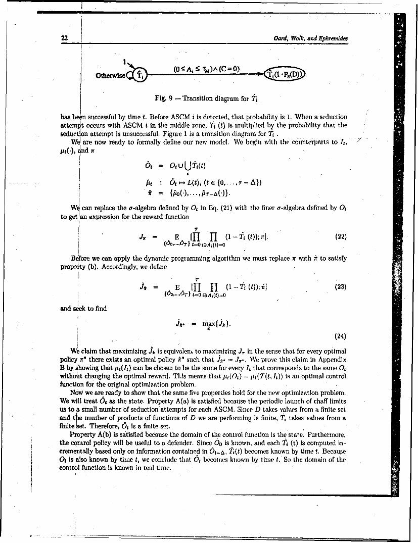
It Is possible to compute t(t) from t(t - A),C(t - A), A,(t - A), and D(t - A) as shown inFig. 9. To see why, recall that Ti(t) represents the probability no seducticn attempt for ASCM i

22 Oard, Wolk, ard Ephrenides

Fig. 9 -- Transition diagram for 2

has be~n successful by time t. Before ASCM i is detected, that probability is 1. When a seductionattempt occurs with ASCM i in the middle zone, tI (t) is multiplied by the probability that theseduction attempt is unsuccessful. Figure 1 is a transition diagram for Ti

Wý are now ready to f'ormally define our new model. We begin with the counterparts to ht "

ju nd 7r

6 = OtuUi(t)i

.fit :6gt - L(t), (t E {0O,....,r -A}

f=

IW• can replace the a-algebra defined by 0t In Eq. (21) with the finer a-algebra defined by Ot

to get an expression for the reward function '

J.r E [YI 1-I 01 - ti (t)); -el. (22).{(o,...,1-1 t=o i9Aj•(t)=o

Before we can apply the dynamic programming algorithm we must replace 7r with ir to satisfyproperty (b). Accordingly, we define

.J* = E II I (1-7 (t)); rI (23){0•7-.,1} t=O i9A,(t)=O

and seek to find

(24)

We claim that maximizing J* Is equivalem to maximizing J, in the sense that for every optimalpolicy ir* there exists an optimal policy r*' such that J*. = J,.. We prove this claim in AppendixB by showing that tt(It) can be chosen to be the same for every It that corresponds to the same Otwithout changing the optimal reward. This means that Ltt(Ot) = pIt(T(t, It)) is an optimal controlfunction for the original optimization problem.

Now we are ready to show that the same five properties hold for the new optimization problem.We will treat Ot as the state. Property A(a) is satisfied because the periodic launch of chaff limitsus to a small number of seduction attempts for .each ASCM. Since D takes values from a finite setand the number of products of functions of D we are performing is finite, Tj takes values from afinite set. Therefore, 6t Is a finite set.

Property A(b) is satisfied because the domain of the control function is the state. Furthermore,the control policy will be useful to a defender. Since Oo Is known, and each tj (t) Is computed in-crementally based only on information contained in O6,-&, tj(t) becomes known by time t. BecauseOt Is also known by time t, we conclude that Ot becomes known by time t. So the domain of thecontrol function is known in real time.

On As hqrwed Schedufing of Hadkil ard SofU 23

The transition diagram in Fig. 9 Is deterministic, and Fig. 8 can be used to determine the nextstate function for Ot without knowledge of th,' outcome ot stochastic transiltions of Ti. So propertyA(c) is satisfied as well.

To apply the dynamic programming algorithm we define

[00 (1-T(t))Vt E {0,.. .,r). (25)i9A,(9)=O

This allows us to rewrite the reward function in the form rcquired by property (e):

Tj* E E I g,(Of); *i{o6,...,o6T 1 =o

This quantity can be computed based only on 6,, and it is nonnIgative blecause it is a probability.So properties (d) and (e) are satisfied. Since all five properties in Appendix A are satisfied we maywrite:

S= r(0T) (26)= max ( E 1 +A(Es+A).t((g);4d(g)1}, ( 0 , {0A.... ,.-A)) (27)

{hU(68)} {6 ,+A)

J.* = E IýVo(Io)1. (28)

5 DYNAMIC PROGRAMMING IMPLEMENTATION

Three well-known ways have beez, developed in which dynamic programming equations can beused to find optimal controls. The equations can be used to develop analytic proofs of optinla!ity,or they can be used in one of two numerical techniques: policy itelation or value iteration. In thefollowing paragraphs, each of these approaches are described. Because it is the most straightforwardof the three, we then consider value iteration in detail. Applicability of the other two methods tothis problem is a topic for future research.

Because we have shown that any policy that satisfies Eqs. (26), (27), and (28) is optimal, this sr,of equations can be used to test candidate policies for optimality. One way to apply this observationIs to develop a policy through some independent technique aild then to attempt to construct ananalytic proof that the control applied for every state at every time is a maximizing control inEq. (27). While such an approach is probably only feasible for relatively simple policies, it offersthe possibility of avoiding a computational implementation altogether.

Howard has developed a comnutationally efficient technique called policy iteration that takesadvantage of the fact that the dynamic programming equation can be used to define a contractionmapping in policy space 12]. His approach was developed for models with a long-time horizon anda reward function that is formed as the sum of a set of stage rewards. Beginning with an arbitrarycontrol function and an arbitrary assignment of rewards for each state, the policy iteration algorithmIteratively applies Eq. (27) to develop a more nearly optimmi control function and the i.s.siatedrewards. Although this "policy iteration" must continue until a fixed poiht is reached, Howardreports that the algorithm often converges after just a few iterations.

Howard's policy iteration algorithm computes each succeeding control ftuiction by solving a setof linear equations. For reward functions formed ais a prodllct of a set of stage rewards, sch aswe have In our model, It is not clear that a practica! analogue to this approatch can be developed.Furthermore, we would expect that reformulation of our model to incorporate a longer time hori-zon would significantly alter the optimal policy choice. Nonetheless, it may prove worthwhile to

/m

/ -

24 Oard, Wolk, and Ephremides

Investigate further the application of policy iteration to this class of reward functions given theproblems that we describe below with Implement at ion of the value Iteration technique.

Equations (26), (27), and (28) can also be used directly to c'alculate the optinial control for

each state at each time. Conceptually, this approach k quite simple. First. the results or Eq. (26)are computed and stored for each state. Equation (27) is then appilcl tio each stat,, iterating this

operation backwards in time until time 0 is reached. At each time the optimnizing policy for eachstate is stored in an array. Finally, the given distribution On the initial state is used to find the

expected reward by applying Eq. (28). This tcchnique is known as value iteration. In the remainderof this report we describe the implementation detail: and the resulting computational complexity

of value Iteration dynamic programming.

5.1 State Coding

Because each state must be considered at each time, reducing the cardinahity of the state spaceproportionally reduces both time and space requirements. For this reason, redundant informa-tion should be removed from the state before coding the algorithm. Redundant information isinformation that would not affect the value of the reward function if it were deleted.

Two types of redundant information exist in our model. The most obvious type is representedby unreachable states. Certain state variable combinations will never be reached, regardless ofthe control policy or the outcome of random events. For example, in the engagement model it isnot possible for a SAM to be in flight (S > 0) when the SAM inventory Is at its maximum value(N = No) since launching a SAM decrements N. Other state variable combinations can occur atsome times, b, not at others. For example, since only one SAM can be launched at each timestep, N cannot reach 0 until No time steps have elapsed. So the set of unreachable states varieswith time.

A more subtle type of redundant information is represented by states that can be excludedwithout changing the value of the reward function, although the policy that achieves that rewardfunction may change. We call these states redundant states, because, although they are initiallyreachable, the optimization problem can be reformulated in a way that makes them unretWhable.Often, more than one policy will result!in the same rew,..rd. We define policies that result in thesame reward to be equivalent and use ýiis relation to partition the policy space into equivalenceclasses. By introducing additional consiraints on the control function, we may reduce the size ofsome of these equivalence classes while intreasing the number of unreachable states. As long as onepolicy remains in the optimizing equival ce ch ss, the dynamic programming algorithm presented

---above will find it. . .. .A simple example may help to clarif this somewhat abstract concept. Consider an instance of

the engagement model with one ASCM that is known to arrive at time 0, one SAM (i.e., No = 1),and no chaff (i.e., Co > -). Since PK is constant, the one SAM could be launched at any time thatwould allow It to reach the ASCM while the ASCM is in the middle zone. Every such policy wouldresult in the same reward in the model we have presented. So every policy with exactly one SAMlaunch between time 0 and time rM - *s is in the optimizing equivalence class. Introducing theconstraint (t < rM - f.) =o, L = Hold reduces the optimizing equivalence class to a single "Don'tshoot until you see the whites of their eyes" policy and makes every state with S > 0 unreachablebetween time 0 and time rM -

Because we have not developed a general procedure to recognize redundant states and craftcontrol constraints that make them unreachable while preserving at least one policy in the opti-mizing equivalence class, an ad hoc approach has been adopted here. As our examp!-; shows, thechoice of constraints and the resulting set of unreachable states depends on the values of the modelparameters (consider how different the result would have been with Nu 2). For this reason, wehave chosen not to pursue the issue of redundant states further.

OA dAs Jnttrated Scheduiin of Hardk&lI and Sofik 25

Unreachable states are more easily recognized and eliminated because no new control constraintsare required. In the engagement model, Tj E Ot until the first seduction attempt occurs with ASCMi in the middle zone. But knowledge of T, is never required to find the next state, and it is neverused to compute ji. So we can calculate J* by using Eqs. (26), (27), and (28) without ever knowingTi. This means that by simply eliminating T, from the state (or equivalently forcing it to a fixedvalue) will change neither the policy nor the value of the iewaird function.

Similarly, C can be eliminated from the state because it depends in a known way on time,regardless of the policy employed. It is included in Fig. 8 simply as a notational convenience. OnceCo, C,,. and t are specified; we can compute C as:

(t<Co) C=C0-t

(t _>Co) •C = (Co -t) mod C,,,,z.

The remaining state variables (N, S, D, Aj, and 1) are all influenced by the control policy andare used in the computation of the reward function. The variables Ai and T, are used directly tofind jt(Ot), while D Is used to find Ti, S is used to find D and to find the distribution on A,, andN is used to constrain the control function. It Is still possible to find combinations of these statevariables that cannot occur, however, as our first example in this section demonstrates.

Since the set of reachable states changes over time, a thorough search for unreachable stateswould require extensive analysis. The most general approach to eliminating unreachrble stateswould be to enumerate the reachable states and map each reachable state to an index in thisenumeration. As was the case for redundant states, however, unreachable states can be difficult torecognize In advance. We cannot use the dynamic programming algorithm to discover which statesare unreachable because the algorithm proceeds backwards in time. Once we discovered that a statewas unreachable, the work we sought to avoid would already have been done! A tree walk woulddiscover which states are reachable, but it would also find the optimal policy (at great expense),obviating the need for dynamic programming. So again we are reduced to an ad hoc approach toeliminating unreachable states.

Programmers must also balance the potential savings obtained from encoding the state againstthe time and space required by the coc'ing and decoding operations. Unreachable state variablecombinations that have simple specifications in terms of existing state variables are easily elim-Inated. Those that require complex specifications or computationally expensive transformationson the state space may not be worth eliminating even if they could be specified. Using this ob-servation to guide our search, we have found no combinations beyond the example given above((N = No) =- S = 0) that apply for all possible model parameters.

5.2 Data Structures

The dynamic programming algorithm iteratively uses the expected partial reward for everystate to find the expected partial reward for each state one time step earlier. Because the partialrewards represent an expected probability of survival, they are real numbers between 0 and 1. Sowe will need at least two floating point arrays. No more than two arrays are needed because onlythe present partial rewards are required to find the partial reward for each state one time stepearlier. We simply alternate between the two arrays to represent the present time step as we iteratebackwards in time.

If our goal were simply to discover the optimal expected probability of survival, these two arrayswould be sufficient. The dynamic programming algorithm will, hlivever, also identify a policy thatrecults in this optimal reward. Storing that policy requires an array index 41 by both tirte andstate. Because the launch control is binary valued, a Boolean a!*ray will sufhl

//

/

26 Oard, Wolk, and Ephremldes

5.3 Algorithm Implementation

While Eqs. (26), (27), and (28) can be used to compute the optimal policy, two simplificationscan reduce the implementation effort. If we define 17r+a(Or+a) 1: I VOr+&, Eq. (26) becomesa special case of Eq. (27). Unnecessary computations are easily avoided by choosing an arrivaldistribution with no arrivals at time r and adopting a constraint that prevents SAM launches attime r. Since 0o is known, Eq. (28) can be replaced with Jf, = Vo(Oo). So all we must compute

Is:S=m ax { E Iýc+a(Ot+A) ' t(Ot); At(Ot)]}, (t E {0..... . (29){•(0aQ)} {Og+&}

To cbmpute this quantity, we must find the distribution on the next state given the presentstate and the control. At each time, Eq. (3) can be used to compute the probability of detectingany particular number of ASCMs for each state. Figure 8 can also be used for each state to find theprobability that a SAM will kill the closest ASCM. Because we have modeled these as independentevents, we can then compute the probability of each possible random outcome. For each possiblecontrol the other state variables make deterministic transitions that are stw( (cifed In Figs. 8 and 9.

Only control values that satisfy the constraints on the launch control need be considered. We donot allow another SAM to be launched if a SAM is already in flight (S > 0), the SAM inventory.isexhausted (N = 0), or the final time has been reached (t = r). If one of these conditions holds, weonly consider L(t) = False. Otherwise, we choose the control that maximizes Eq. (29). Specifically.we compute:

Vljstatelj = max I{ Pr{transition from statel to state2 ; Listatell I{L[statellh state2

•V2[state2] 1- (1 -ii in statel)} (30)siA,=o in statel

where V1 Is the array of partial rewards at the prior time, V2 is the array of partial rewards at thepresent time, and L is the slice of the policy array for the prior time.

We are now ready to tie up the loose ends and present the algorithm. The time variable t isinitially set to r, and every value in V2 is set to 1. Vl[state 11 is then calculated by using Eq. (30)for each state 1 at time t and the maximizing Lfstate 11 (either Tifue or False) is stored in the policyarray for state 1 at time t. Once Vl[state 1] has been computed for every state, V2 is replaced byVi, t is decremented by A, and the process repeats using Eq. (30). This time VT-,a(.) and 4r-a(.)are computed. The iteration continues until the pass for t=O has been completed. The value of4J. can then be read from Vl[state 1] for the value of state 1 that corresponds to the known initialvalue of Oo. The policy array will contain a specification for a SAM launch policy that would result -. . ...In this expected probability of survival.

5.4 Computational Complexity

The dynamic programming algorithm requires that for each control all of the states that canbe reached from every state at every time be considered. Therefore, the number of operations thatmust be performed is directly proportional to the number of controls times the fanout from eachstate times the number of states times the number of time steps.

The fanout is the number of states that can be reached from a given state in one time step fora specified control. Since at most m + 1 ASCMs can arrive simultaneously and states that includean Intercept (i.e., S = 0) could lead to one of two different states for each possible number ofarrivals, the maximum fanout Is 2(rn + 1). Most states do not, however, include an intercept andmost restrict the maximum number of arrivals to fewer than m ASCMs because some ASCMs have

M.- _. .asltv &he...ing of Hardkii•lAd f ..

already been detected. For this reason, Me is probably a closer estimate of the average fanout.For the parameters in Table 2, an average fanout of approximately 2 would be expected.

The number of states turns out to be very large:

A, There are •'+ useful values for each Aj. Those values are I-oo, A, 1,..,rM,00)}. Otherpositive numbers do not occur. All negative numbers can be mapped to -oo because doingso preserves the effect of A, on each branch of every transition diagram in Figs. 8 and9. Since there are m ASCMs, there are (,(,"+3)", possible values for (A,,..., Am}. Theparameters In Table 2 result in 51 possible values for each Aj, or 1.3 x 105 possible values for{A,,...,A)}.

D There are DPa- + 1 useful values for D. Those values are (0. A...., D,,}. Negative numbersdo not occur. Other positive numbers can be mapped to D,,. because the definition ofD,,. ensures that (D > D,.) =:. Ps(D) = Ps(D,,.). The parameters in Table 2 result in9 possible values for D.

N There are N0 + 1 possible values for N. They are (0, 1,...,No). The parameters in Table 2result In 6 possible values for. N.

There are AMJ + 2 useful values for S. These values are {-oo, 0, A,... A• ' J. FigureeL ! 7 m s+ T} Fs_ i g u r

8 shows that the larest. posibbe value for S is ti(t)- t. Substitution of the maximum possiblevalue for Ai In Eq. (4) yields A L -MMi1)j for this value. All negative numbers can be mappedto -oo because doing so preserves the effect of S on each branch of every transition diagramin Figs. 8 and 9. The parameters In Table 2 result in 17 possible values for S.

Td Since there are !- + 1 time steps and f + I time steps elapse between each seduction. therecan be at most r seduction attempts. The transition diagram in Fig. 9 shows that7 will be multiplied by a function of D (which could assume one of • + 1 values) ateach seduction attempt. Since an unsuccessful seduction attempt (D = 0) results in the samevalue as no seduction attempt, D = 0 can beused to represent either situation. Becausemultiplication is commutative and associative, there are as many possible values of T, asthere are choices (with replacement) of values of D for each seduction attempt. Since thereare m ASCMs, there are at most in times this number of possible values for {To .....This value can be computed as:

The parameters in Table 2 result In at most 3 possible seductions and 9 possible values for Dat each seduction attempt, resulting in 129 possible values fort,, or 2.1 x 106 posib)le valuesfor Ito,

Multiplying the values for the parameters in Table 2 together, we find there are over 2.6 x 10"4

possible states. Since (N = No) =* (S = 0), a slight reduction to approximately 2.2 x 10t4 statescan be achieved by coding N and S together.

Because the launch control is binary, the maximum number of possible controls is two. Theconstraint that precludes a SAM launch when a SAM is already In flight makes the average numberof controls much closer to one, though, because S > 0 in most of the states. Finally, there are'r + 1 possible time steps. For the parameters In Table 2, there are 148 possible time steps.

Combining these results, the dynamic programming algorithm reqnires retrieval of approxi-mately 6.5 x 101s floating point numbers from memory and requires us to perform a prop(rtionalnumber of arithmetic and logical operations. Even with a 10 gigabyte per .m'onl lmemory 6vid-

28 Orrd, Wolk, and Ephremides

width it would take over two months to simply perform the required memory accesses. Each ofthe two floating point partial reward arrays contains approxihmatelv 2201 trillion values; together,they require about 1800 terabytes of random access memory when Stored with single precision.

The policy array consists of approximately 220 trillion bits for each of the 148 time steps, andthey require over 4000 terabytes of offiine storage during the computation and an equal amount ofrandom access memory during policy employment.

The strength of value iteration dynamic programming is that it provides an exact global solutionfor combinatorial optimization problems without resorting to exhaustive search. For the model wehave developed above, the computational complexity of using dynamic programming in this way isobviously well beyond the capability of existing computer systems. In the following discussion wewill describe two alternative approaches for resolving this dilemma. First we consider the potentialfor restricting our model in ways that will result in improved implementation efficiency. Since itremains an open question whether the approaches we describe below retain suffIcient fidelity toallow application of value iteration dynamic programming to practical problems, we conclude witha brief discussion of potential for developing heuristic optimization techniques for these problems.

5.5 Reducing Computational Complexity

The four factors contributing to the complexity of the dynamic programming algorithm arethe number of states, the number of available controls in each state, the fanout from each state,and the number of time steps. There is little'point to further constraining the number of availablecontrols in each state because only one possible control exists in most of the states and no morethan two controls are possible in any state in our model. However, we can gain significantly byreducing the number of time steps. The number of time steps can be reduced by increasing Aor by introducing an assumption such as clustered arrivals that would allow r to be decreased.Furthermore, increasing A would significantly reduce the number of states and clustered arrivals,and would also reduce fanout. Thus we begin by considering changes that reduce the number oftime steps and then discuss other assumptions that could be introduced to reduce the state spacestill further.

5.5.1 Time Step Reduction

The value of A in Table 2 results in a separation between values of D that is appropriate to theaccuracy with which data for Ps(D) was collected. Increasing A results in coarser coding for D,leading to a less accurate estimate of seduction effectiveness. This decreased accuracy could leadto a overdependence or underdependence on the chaff, depending on the type of error introduced.Thus, a significant increase inf A could make the results of the optimization less useful.

In addition to reducing the number of time steps, increasing A also reduces the number ofpossible values for every state variable except N. For the parameters in Table 2, the number ofpossible states decreases with the eighth power of the factor by which A is increased. Doubling Awould reduce the number of possible states by a factor of 256. Coupled with the time step reduction,the computational complexity is reduced by the ninth power, a factor of 512 for doubling A. Thisextreme sensitivity to A places great weight on the choice of the maximum practical value for this

- -parameter.

The potential improvement resulting from reducing r is less dramatic. We consider an engage-ment to begin when the first ASCM is detected. The value of r in Table 2 is sufficient to find theoptimal policy regardless of the subsequent ASCM arrival pattern, subject only to the requirementthat every ASCM shares the middle zone with at least one other ASCM for at least one timeinstant. It was found by considering the case in which each subsequent ASCM is detected just asthe prior ASCM reaches the inner zone. We have not considered the case of ASCMs that never

On Ba Ihupared Scheddng of HardkilZ and SoftUl 29

share the middle zone with another ASCM because that case is easily handled by decomposing themultiple ASCM engagement into a sequence of single ASCM engagements. The optimal policy forthe multiple ASCM engagement could then be found by sequentially finding the optimal policy foreach single ASCM engagement.

Restricting all arrivals to the first few seconds of the engagement would reduce r by a factorbetween 2 and 3. This is a reasonable restriction because clustered arrivals are known to be aneffective attack technique. Restricting ASCM arrival times in this way, times also reduce theaverage fanout from around 2 to a value close to 1. Taken together, this approach offers a factorof 5 Improvement in speed and a factor of 2.5 improvement in the number of states.

5.5.2 State Space Reduction

Together, the two approaches to time step reduction could yield a performance improvement ofabout three orders of magnitude if, for example, analysis shuwed that A could safely be doubled.Even with that speedup, additional improvement would be required before a practical implementa-tion could be developed. One approach is to simply eliminate the inventory constraint. If enoughSAMs were available to the defender to assure their availability throughout the engagement, thechoice of controls would not depend on the Inventory. Thus the state variable N could be deletedand the SAM launch constraint simplified by eliminating the N > 0 requirement. For the parame-ters in Table 2, this would reduce the number of state variables by a factor of 6.

A bolder approach would be to arbitrarily reduce the precision with which a state variable isrecorded. While this approach cannot be applied to counting processes such as N, S and A,, itoffers great promise when applied to Ti. Initial experiments with the parameters shown in Table 2(with a restriction to clustered arrivals to speed execution) show that approximately 10 evenlyspaced values are sufficient to compute a value for J,. that is accurate to within 0.05 of the valuefound when exact values were used. Such coding results in 1,000 possible values for {To_. , Tm}a reduction by a factor of over 2,000 compared to the number of possible values for exact coding.Unfortunately, the policy found in this way could differ significantly from th, optimal policy foundby using exact coding. Additional research is required to understand how quantizing T, affects theoptimal policy and to find the best quantization algorithm.

In summary, eliminating the inventory constraint and clustering arrivals would reduce the coin-putatlonal complexity by one order of magnitude while retaining the ability to accurately model awide range of realistic engagements. By taking these steps and doubling A and quantizing T, to 10values, we could achieve a seven order of magnitude improvement over a model with the parametersshown In Table 2. This improvement comes at the expense of some loss of accuracy that remainsto be quantified, but It allows a solution to be calculated for a problem with parameters similar tothose In Table 2 without placing Impractical demands on computer resodrces.

6 FUTURE RESEARCH

Practical ship defense systems will require models that incorporate additional dynamics and awider range of parameters. In practice, ASCM seeker parameters may not be uniform, and may notbe known a priori. Other defensive systems must be integrated with the two considered here. Andprotracted engagements consisting of several waves of ASCMs may have to be addressed. Theserequirements would yield larger state spaces and greater fanout, and may require many more timesteps. Even the Improvements of the type just described offer no practical hope for dealing withthis sort of computational complexity.

30 Oard, Wolk, and Ephremidets

"The simplifying assumptions in Section 5.5 alone will not be adequate for models of this com-plexity. The principal advantage of the dynamic programming algorithm desc'ibed in this reportis that it produces an optimal solution without considering the alternatives available in each stateat each time more than once. Its principal limitation is that we must perform the computation forevery state, regardless of whether the state is reachable, This limitation arises because we Workbackwards in time in the d)namic programming algorithm, and hence we are unable to recognizeunreachable states during the computation. A forward tree search for the optimal policy avoids"evaluating unreachable states at the cost of greater time or space complexity. To apply dynamicprogramming to these more challenging models would require the Investigation of other uses ofthe dynamic programming equations such as policy iteration and analytic proofs of optimality. Ifthese techniques do not prove to be feasible, it will be necessary to consider heuristic optimization

* / techniques.A number of heuristic techniques that have been applied to similar problems appear to offer some

promise for application to the ship defense problem. SAMUEL is a computer program developedby.the Navy Center for Artificial Intelligence Research that uses a genetic algorithm to develop aspecification for a near-optimal policy. [3]. Policies in SAMUEL are specified by a set of rules thatare used to select controls based on observations. The genetic algorithm in SAMUEL adds, deletes,and changes those rules in an attempt to improve the value of the reward function. Application ofSAMUEL to the ship defense problem would require the creation of a world model that is used bythe simulation module in SAMUEL to evaluate candidate policy specifications.

The effectiveness of the technique used by SAMUEL depends on the suitability of a relativelysmall rule set for specification of near-optimal policies. Because we expect to be able to achieve anoptimal dynamic programming implementation for our limited engagement model described above,evaluation of SAMUEL's performance on that model should be straightforward. Furthermore, wewould hope to gain some insight Into the usefulness of policy specification using small rule sets.Although the policy array is generally far too large for online storage, small rule sets would beuseful in developing online decision aids and tactical guidance for defensive system operators.

Another technique worth investigating is a limited lookahead forward tree search. Rather thanevaluate every path through the complete state space, the number of time steps to be consideredIs sharply limited and a heuristic evaluation of the partial reward is performed for each state whenthat limit is reached. By limiting the depth of the tree search we can avoid both considerationof unreachable states and extensive reconsideration of the same state. This approach is similar tothe technique used by computer chess programs; however, the introduction of stochastic transitionscould result in some significant differences in the implementation of the c.oncept. I

Selection of an appropriate heuristic for the static evaluation of terminal states is critical tothe performance of the limited look ahead technique. One possible heuristic would be to use thesame reward that SAMUEL wouid use to evaluate candidate rule sets. SAMUEL determines theperformance of a set of rules from a known starting state by Monte Carlo simulation. To useSAMUEL's approach for static evaluation of an intermediate state, SAMUEL would first be usedto find a good set of rules, and then SAMUEL's simulation module would be appli( - to the statebeing considered. to find the expected performance of that set of rules starting from the specifiedstate. An adva.itage of the limited look ahead technique is that it might be possible to applyit in real time rather than developing a policy off-line. If rules turn out to be poorly suited forspecifying near-optimal policies, real-time policy development may be the only practical alternative.The availability of an optimal dynamic programming implementation for the engagement modelwould also facilitate performance evaluation in this case.

On Us Ipated Sckhisdu of HardJ and Softi 31

A third approach that could be useful, if small rule sets are not found to be effective, is todevelop a neural network that could generate near-optimal controls. In one such approach, abackpropagating neural network could be trained off-line by using an optimal dynamic programmingsolution for a limited engagement model and then it could be used in real time to generate theoptimal controls. Werbos has proposed using backpropagation through time to train the worldmodel of a backpropagating adaptive critic 141.

Finally, Hopfield neural networks offer the possibility of directly developing an optimal policy,if a short binary specification for a policy could be developed. The rule set developed by SAMUELmay provide some insight into the development of an appropriate policy representation.

7 CONCLUSION

Because value iteration dynamic programming requires that we work backward in time, wemust consider every combination of state variables at every time. Although we may be able to findan optimal solution for a small problem using dynamic programming, solving problems based onlarger models requires more computer resources than can practically be provided. For this reasonwe are motivated to search for faster techniques. Both heuristic techniques and alternative usesof the dynamic programming equations bear further investigation. The value iteration dynamicprogramming solution we have developed is useful, however, since it can be used to gain insightinto the design of such algorithms and to evaluate the performance of those algorithms in a restricteddomain.

REFERENCES

I1] K. M. Potter, "Optimal Resource Allocation for a Controller with Two Resource Types," NRLMemorandum Report 6553, October 1989.

12] R.A. Howard, Dynamic Programming and Markov Processes (Wiley and Sons, New York, N.Y.,1960), pp. 32-43.

131 J. J. Grefenstette and H. J. Cobb, "User's Guide for SAMUEL, Version 3," NRL MemorandumReport, January 1993.

[4] P. J. Werbos, "Backpropagation and Neurocontrol: A Review and Prospectus," InternationalJoint Conference on Neural Networks. Piscataway, N.J.: IEEE TAB Neural Network Commit-tee, 1, 209-216 (1989).

151 D. P. Bertsekas, Dynamic Progrcmming: Deterministic and Stochastic Models (Prentice-Hall,Englewood Cliffs, N.J., 1987), pp. 12-22.

Appendix A

DYNAMIC PROGRAMMING WITH MULTIPLICATIVE REWARDS

A.1 GIVEN

"We are given an initial time 0, a constant time quantum of 1 arbitrary unit, a nonnegative integer

final time T, random variables {Xo, .. , Xr} taking values {xo,..., xr} that represent states, a class

of control policies 7r = {(',.... ,Dr-l()}, and a reward function J, with the following properties:

(a) xt E Xt V(t E ...... , r}), -where Xt is a finite set that represents the possible states at

time t.

(b) : Xt U-- UV(t E {0,. .. ,T - 1)), where U is a finite set that represents the available

controls. Furthermore, pt(xt) E Ut(xt) V(t E {0,..., r - 1)),V(xt E Xt), where Ut(•t) is a

finite set that represents the admissible controls at time t if the state is xt.

(c) The distribution on Xo is given and the distribution on Xt+l is completely determined

by xt and j(xt) Vt E {0,...,.r- 1}:Pr{Xt+i =' t+,lXo = xo,... xt = xt; o(),... ()

= Pr{X,+i = Xt+ilXt = Xt;At(xt)}

By, for example, Pr{Xt+l = Zt+1 IXt = xt; pt(xt)} we mean the probability of the event

{Xt+i = xt+i} conditioned on the event {Xt = xt}, given the value of pt(xt) as a

parameter.

(d) At each time t E {0,..., 7.), a nonnegative reward factor g9(xt) that depends only on the

present state xt Is computed.

(e) The overall reward is the expectation of the product of the reward factors (and is a

function of the control policy 7r): 1"J.1= E flgt(Xt)]

{xo,...,x'r) 9=0

Our goal is to find the maximum reward that can be earned over all admissible policies and a

policy which earns that reward. Formally:7.

ma= x{ E .I] g,(X,)l)xoO...,-x1, t=O

1*

*= arg i {...ax E I.Tgt(X,)l){X0.-- XT) t=0

Where we maximize over ir we mean maximization over pt(xt) E Ur(xt), V(t E {0 ..... r- 1)), V(xt E

xe).

33

3I 4 Oard; I olk, d EphremIdes

A.2 CLAIM

Property (e) defines a reward function with a multiplicative structure. For reward func-tions with an additive cost structure, the dynamic programming algorithm described by Bertsekasin 151 provides a solution technique with a time complexity that Is 0(r). Here we describe ananalogous algorithm for a multiplicative reward function.

We define a set of functions Vt(xt) as:

VT(Xr) = gr(Xr)Yzz,) = 9&(t), max( E IV,+,(X,+j)]}, (tE E{0,..., 7- 1)),

pt(zt) {X,+ 1}

and then claim we can compute J,. as

J.. = E (Vo(Xo)].(Xo)

Furthermore, we define:

At(xt) = arg ma({ E IV,+IXt+ )]}, (t E {o,...,r- 1)J11(29) {V1+11}

*t = {•,()} U *+I, (t E (0,... ,r - WS),

where 0 represents the empty set, and claim that

7r* = fr0.

A.3 PROOF

We begin with the special case of r = 0. Here the result follows directly from the definitions

0,max E flIg,(x,)J}

SVXol t=0

= E [go(Xo)J{xo)

= E lVo(Xo)l.• {xo)

Thus we may focus our attention on the case in which -r > 1. We will show by induction on nthat Vn E {0,...,iT- 1)

en

E lVo(Xo)I = max... max{ E IVn+,(Xr.+,) 'l[9,(Xt)-1Xo) Ito(-) P-({Xo...,X.+u =o

For the basis case we will take n = 0 and show that

0

E o}Vo(Xo) = max{ E IV(Xi) Igt(Xt)IVX) po(.) {Xo.X) t=o

= max( E [V,(Xi).go(Xo)].Mo() {Xo,X,)

On Integratrd Schedading of Hardkill and Sofikill 35

Expanding the left side by using the definitions of Vo and expectation, bringing two nonnega-tive constants Inside a maximization and a summation, and then interchanging maximization andsummation

E (VO(XOfl"= E Lgo(Xo). max{ E [Vi(XI)]}]

V{Xo) " o(Xo) (X1)E= Pr{Xo = xo} -go(xo) max{ • Pr{Xi =xjXo =xo;po(xo)}. V,(xi)}

ZoEo U-O(Xo) xlr=X

. / max({ E Pr{Xi =zlXo0=x0;po(xo)}.Pr(Xo=xo}'VI(x) 'go(xo))zoECXhPo(zo) zlexi

=max.{ , E Pr{X, =xlXo=xo;po(Xo)} .Pr{Xo=xo). V,(x,).go(xo))"POO zoEXo ziExi

This last step requires some justification. With the maximization inside the summation we areseparately choosing the values of po(xo) that maximize each term of the summation. Maximizingoutside the summation requires us to simultaneously choose values of Mo(.) for every possible valueof Zo that maximize the sum. In this case the two operations are equivalent because each choiceof Po(xo) affects at most one term of the sum. In particular, property (c) ensures that Pr{Xi =ziIXo = xo; po(xo)} depends on no other choice of uo(.). Also note that V, (xj) does not vary withpo(zo) because no Information for earlier times is used in the construction of Vt. In general, we canexchange maximization and summation in this way whenever the index of the outer summationassumes values from the domain of the function over which we are maximizing; each term in thesummation depends on the value of the function over which we are maximizing for at most oneelement of its domain, and the value of the function for each element in its domain affects at mostone term in the summation.

To complete the proof of the basis case we apply the definitions of conditional probability andexpectation

E jVo(Xo)l(XO)

= max Pr{X,=xi,Xo =xo; o(xo)1 V,(xi).go(xo)}zoE•o zxEXi

= max E [Vd(xm).go(Xo)J).PO() (Xo,X1}

We now take as our Inductive hypothesis for n E {1, .... r - 1}

n-1E [Vo(Xo)] = max... max I E IVn(Xn) 1i gt(Xt)]

{Xo) Po() M,,-(.) Xo..,X) t=o

and show thatn

E [Vo(Xo)] =max...max{ E IV,,+I(Xn+,)" 10gt(X0).{Xo) pO( '".0) {Xo,...,X,+ 1 t=o

We begin by separating the expectation on the right side of the inductive hypothesis, bringinga constant outside the inner expectation, expanding Vn, and bringing two nonnegative constantsinside the Inner maximization:

36 Oard, Wolk, and Ephrewdda

E IVO(Xo)l(Xo1

n-I

= max... max { E IV.(X.). fI g,(Xt)ll0•(.) O ,,-(.){Xo,.-.x, } -o

= max... max{ E I E IVn(X,). ,(Xt)ll}POO -,. ix.) {Xo....,x '-,} 9--o

n-|= max... max{ E [Vn(Xn) E Ifl-gt,•X)1J)

P(-) P-0(.) {x,) {Xo,...,Xn. 1} t=on-I

= max... max { E Ign(X.). Max ( E IVn++(X.+,)))) III gt(X,)H}U0o(. I (X.) Po(X.) (X ) {XO..x,-, t=0

n-1= max... max { E [max ({ E !V+ I(X,)+i) .+ g.(X.) E I-H g,(X0) }1}.

P.00 p,-IO {X,) ,,(Xn) {XXo,....X)- t=0.

Now observe that the expectation over X, is taken on an expression that depends on only onevalue of /4(Xn). Viewing the expectation as a weighted stun, the index of the summation assumesvalues from the domain of the function over which we are maximizing; each term in the summationdepends on the value of the function over which we are maximizing for at most one element of itsdomain, and the value of the function for each element In its domain affects at most one term inthe summation. So we can exchange that expectation with the inner maximization. Doing this andmoving constants inside expectations

n-1

E [Vo(Xo)J = max...max{ E I E lV,+,(X.+,)l9g,(X.). E IIgt (Xt).(xO) POW A-0.(n) {x (n+} JXU ... i. g(X)=0n-1

= max ... max{ E I E ([V,+ 1(X.+1) •(X-). E I'i g,(XV)!1}o() {X {X.+) jXo,.'..X.-} 9=o

n-1= Max... max( E I E I E IVn+,(Xn+|)• -9n(Xn) •1 gt(X,)llJ}.

POO ( ( .) 1X.+4 { ,,+iI{xo . 0. =o

Combining the expectations and the product of the reward factors completes the Induction

E IVo(Xo)i = x...max{ E IV.+I(X 1),). 1 ,x,).{XO) U(.) ('.) {o..0.,X +1 1=0

Choosing n = -r - 1 and applying the definitions of Vr and 7r

"7-IE iVo(Xo)I = max... max ( E IV((XT) f' g1(X01){XO POO. P,-,0(') {o....x }X) =

X0=0

1"= max{ E I lgt(Xt)I1i"O.'"?*TI 8=0

- X,..r 1=0.

This proves the first claim. The proof of the second claim follows the same approach with moreattention tn the identity of the maximizing control functions =t().

On the Integrated Scheduling of HardkiU ard Sofikil_ 37

Appendix B

EQUIVALENCE OF THE SIMPLIFIED POLICY

We claim that maxhaizing J4 Is equivalent to maximizing J, In the sense t at for any optimalpolicy 7r* there Is an optimal policy ** such that

j,*. = J.1

To prove this, it suffices to show that %'o(Oo) iVo(o)A Vo 6= Oo. To accomplish this, we

will prove by Induction backwards on't from r to 0 by A that

v,(~ ( Vit), V1~ E {O..... ,r) V6tVht D6 = Tt t.

For the basis case, we begin with Vr(Ob) and apply Eqs. (26), (20), (19), (6) and (17) to get

'070) = rj (1-4 (Tr))I{iDA,(7)=o}.

= VT( I7)

which proves the basis case. For the inductive step we assume

t+A(OL+a) = V+(1it+&), V V(h+A V E t+a ='(t + A, It+&)), t E {A,..., 7 - A}

and must show thatfr(60)= Vt(it), v~t Wit B 6 T(t, It)).

Let Ot be arbitrary. Then, by Eqs. (18), (16), (19), (20) and the inductive !hypothesis

Vt (it) =max( IVt+AIt+A) f i (1 -t i(t))]}

max J1(+,O+) II ( t))].a(Ih) {(I+A} A(t)=O

Observing that the function inside the expectation depends on no aspects of It+, other thanOg+, and that T(t + A,.) Induces a partition on It+, we can now write:

Vt(It) = max E ( l+,(Ot+,) J (1 -E(t))J}.

When we write pt(It), we mean the control L(t) that is selected at time t. rogether, (Ot andL(t) determine the distribution on Ot+A. Observe, however, that the value 6f the expectationIs a function of the value of Ot and the dismribution on Ot+&. So, while different controls maymaximize the expectation for the same Or, all must result in the same maximal value. Thus,

I i

38 Oard, Wolk, and EphremIdes

any maximizing control may be chosen arbitrarily. Therefore we apply Eqs. (25)and (27) towrite

Vg(lh) = max { E f•+,(6et+A). fl (1 -t )•,(6s) {6'+AI •dt== ((5(+,)

as was to be shown.