NBER WORKING PAPER SERIES

INEQUALITY IN HUMAN CAPITAL AND ENDOGENOUS CREDIT CONSTRAINTS

Rong HaiJames J. Heckman

Working Paper 22999http://www.nber.org/papers/w22999

NATIONAL BUREAU OF ECONOMIC RESEARCH1050 Massachusetts Avenue

Cambridge, MA 02138December 2016

We thank Dean Corbae, Mariacristina De Nardi, Lance Lochner, Steve Stern, and participants at the Human Capital and Inequality Conference held at Chicago on December 17th, 2015, for helpful comments and suggestions on an earlier draft of this paper. We also thank Joseph Altonji, Peter Arcidiacono, Panle Jia Barwick, Jeremy Fox, Jorge García, Limor Golan, Lars Hansen, John Kennan, Rasmus Lentz, Maurizio Mazzocco, Aloysius Siow, Ronni Pavan, John Rust, Bertel Schjerning, Christopher Taber, and participants at the Cowles Conference in Structural Microeconomics and the Stanford Institute for Theoretical Economics (SITE) Summer Workshop for helpful comments. We also thank two anonymous referees. Yu Kyung Koh provided very helpful comments on this paper. This research was supported in part by: the Pritzker Children's Initiative; the Buffett Early Childhood Fund; NIH grants NICHD R37HD065072, NICHD R01HD054702, and NIA R24AG048081; an anonymous funder; Successful Pathways from School to Work, an initiative of the University of Chicago's Committee on Education and funded by the Hymen Milgrom Supporting Organization; the Human Capital and Economic Opportunity Global Working Group, an initiative of the Center for the Economics of Human Development and funded by the Institute for New Economic Thinking; and the American Bar Foundation. The views expressed in this paper are solely those of the authors and do not necessarily represent those of the funders or the official views of the National Institutes of Health. The views expressed herein are those of the authors and do not necessarily reflect the views of the National Bureau of Economic Research.

NBER working papers are circulated for discussion and comment purposes. They have not been peer-reviewed or been subject to the review by the NBER Board of Directors that accompanies official NBER publications.

© 2016 by Rong Hai and James J. Heckman. All rights reserved. Short sections of text, not to exceed two paragraphs, may be quoted without explicit permission provided that full credit, including © notice, is given to the source.

Inequality in Human Capital and Endogenous Credit ConstraintsRong Hai and James J. HeckmanNBER Working Paper No. 22999December 2016JEL No. I2,J2

ABSTRACT

This paper investigates the determinants of inequality in human capital with an emphasis on the role of the credit constraints. We develop and estimate a model in which individuals face uninsured human capital risks and invest in education, acquire work experience, accumulate assets and smooth consumption. Agents can borrow from the private lending market and from government student loan programs. The private market credit limit is explicitly derived by extending the natural borrowing limit of Aiyagari (1994) to incorporate endogenous labor supply, human capital accumulation, psychic costs of working, and age. We quantify the effects of cognitive ability, noncognitive ability, parental education, and parental wealth on educational attainment, wages, and consumption. We conduct counterfactual experiments with respect to tuition subsidies and enhanced student loan limits and evaluate their effects on educational attainment and inequality. We compare the performance of our model with an influential ad hoc model in the literature with education-specific fixed loan limits. We find evidence of substantial life cycle credit constraints that affect human capital accumulation and inequality. The constrained fall into two groups: those who are permanently poor over their lifetimes and a group of well-endowed individuals with rising high levels of acquired skills who are constrained early in their life cycles. Equalizing cognitive and noncognitive ability has dramatic effects on inequality. Equalizing parental backgrounds has much weaker effects. Tuition costs have weak effects on inequality.

Rong HaiDepartment of EconomicsUniversity of Miami314P JenkinsCoral Gables, FL 33146rhai@bus.miami.edu

James J. HeckmanDepartment of EconomicsThe University of Chicago1126 E. 59th StreetChicago, IL 60637and IZAand also NBERjjh@uchicago.edu

A data appendix is available at http://www.nber.org/data-appendix/w22999

Inequality in Human Capital and Endogenous Credit Constraints

Rong Haia,∗, James J. Heckmanb

aDepartment of Economics, University of Miami, 314P Jenkins Building, Coral Gables, FL, 33146, USAbDepartment of Economics, University of Chicago, 1126 East 59th Street, Chicago, IL 60637, USA; phone:

773-702-0634; fax: 773-702-8490

Abstract

This paper investigates the determinants of inequality in human capital with an emphasis onthe role of the credit constraints. We develop and estimate a model in which individuals faceuninsured human capital risks and invest in education, acquire work experience, accumulateassets and smooth consumption. Agents can borrow from the private lending market andfrom government student loan programs. The private market credit limit is explicitly derivedby extending the natural borrowing limit of Aiyagari (1994) to incorporate endogenous laborsupply, human capital accumulation, psychic costs of working, and age. We quantify theeffects of cognitive ability, noncognitive ability, parental education, and parental wealth oneducational attainment, wages, and consumption. We conduct counterfactual experimentswith respect to tuition subsidies and enhanced student loan limits and evaluate their effectson educational attainment and inequality. We compare the performance of our model withan influential ad hoc model in the literature with education-specific fixed loan limits. We findevidence of substantial life cycle credit constraints that affect human capital accumulationand inequality. The constrained fall into two groups: those who are permanently poor overtheir lifetimes and a group of well-endowed individuals with rising high levels of acquiredskills who are constrained early in their life cycles. Equalizing cognitive and noncognitiveability has dramatic effects on inequality. Equalizing parental backgrounds has much weakereffects. Tuition costs have weak effects on inequality.

Keywords: Human Capital, Credit Constraints, Natural Borrowing Limit, Education,WealthJEL codes: I2, J2

1 Introduction

This paper develops and estimates a dynamic model of schooling and work experience in

which agents are subject to uninsured human capital risks and face restrictions on their bor-

rowing possibilities. We analyze unsecured borrowing limits with endogenous labor supply

and human capital accumulation. We estimate the structural parameters of preferences and

∗Corresponding authorEmail addresses: rhai@bus.miami.edu (Rong Hai), jjh@uchicago.edu (James J. Heckman)

Preprint submitted to Review of Economic Dynamics December 28, 2016

the technology of human capital production. They completely characterize the borrowing

limits for heterogeneous agents. Accounting for borrowing limits in an environment with no

asymmetries in information between lenders and borrowers where agents make consumption,

human capital, and labor supply decisions has important consequences for understanding ed-

ucational choices and human capital investment.

There is a growing body of evidence supporting the empirical importance of credit con-

straints in affecting educational attainment. As noted in Lochner and Monge-Naranjo (2015),

the early literature found little evidence for them. The recent literature – based on more

recent data – shows much stronger evidence for credit constraints, a phenomenon first noted

in Belley and Lochner (2007), and documented in later studies (Bailey and Dynarski, 2011,

Lochner and Monge-Naranjo, 2012, and Johnson, 2013).

Previous empirical research on this topic fixes lending limits at ad hoc values, or else

introduces additional “free parameters” to model credit limits. In our analysis, agents can

borrow up to model-determined limits derived from an analysis of private lending with a

natural limit combined with access to government student loan programs. No ad hoc or free

parameters are introduced.

Ours is the first analysis that extends the natural borrowing limit of Aiyagari to simul-

taneously encompass endogenous labor supply, consumption, human capital accumulation,

and savings in physical capital. Our model predicts that borrowing limits are lower for

individuals who have lower levels of human capital and higher psychic costs of working.

The predicted credit limits vary with age, first increasing, and then decreasing. Following

Aiyagari (1994), we assume that lenders can fully enforce contracts and collect on resources

available to individuals. Borrowers must repay as long as they have resources. However,

different from Aiyagari (1994), agents in our model have the option of not working. Lenders

cannot force borrowers to work and human capital productivity shocks are uninsurable. The

lending/enforcement protocol is that lenders can enforce full repayment subject to the restric-

tion that borrowers must be provided a minimum consumption level that satisfies individual

2

rationality constraints for working.

We use our estimated model to analyze the cross-sectional characteristics and the age

profiles of the borrowing constrained population. We find that credit-constrained agents fall

roughly into two groups: (a) those with poor initial endowments and family background

who acquire little human capital, have low wage levels, and little life cycle wage growth, and

(b) those who are able and from good family backgrounds who have more education, less

work experience, high wage levels, and substantial life cycle wage growth. The first group of

agents is constrained throughout their life cycles. The second group is constrained in their

late 20s and early 30s, although they have high levels of life cycle wealth and human capital

and rapid wage growth. They cannot fully smooth consumption in the early stages of their

life cycles.

There is a corresponding two-humped profile of constrained agents with respect to en-

dowments and abilities at the early stages of labor market entry. As income is harvested

over the life cycle, the second hump (associated with the second, more affluent group) dis-

appears. The first group with poor initial conditions remains constrained over its lifetime.

This group of individuals has low labor market earnings, little savings, and small borrowing

limits. Persons in this group have high discount rates and thus are less patient. They want

consumption upfront but cannot access it due to their low borrowing limits.

Our paper extends the existing literature in other dimensions by analyzing how cognitive

and noncognitive ability affects choices through (i) psychic costs of working and schooling;

(ii) the technology of human capital production; and (iii) discount factors. Following Cunha

and Heckman (2008) and Cunha et al. (2010), we allow our measures of abilities to be

fallible. We introduce heterogeneity in parental transfers which is not investigated in the

existing literature.

We use our estimated model to understand the sources of inequality in education, wages,

and consumption over the life cycle. We consider how parental characteristics and transfers,

as well as credit markets, affect choices and outcomes. We find strong effects of adolescent

3

endowments of cognitive and noncognitive ability on human capital development. Tuition

costs and family transfers to children also play important roles in explaining differences in

human capital investments.

We conduct counterfactual policy experiments using our estimated model. We examine

the impact of equalizing initial endowments on inequality in consumption, wages, and human

capital. We also examine the consequences of reducing tuition and increasing student loan

limits on college attendance and graduation.

We compare our model with a recent model in the literature that fixes loan limits by

education level in an ad hoc fashion (Abbott et al., 2016). Using their specification, estimated

subjective discount rates are smaller than in our model with endogenous credit limits. The

goodness of fit is somewhat worse. Comparing counterfactual outcomes, the model with

fixed credit limits by education predicts a higher elasticity of educational response to tuition

than our model with the fully endogenous borrowing limit. The ad hoc model also predicts

a much larger effect of increasing student loans on college enrollment and 4-year college

completion.

The rest of the paper is organized as follows. Section 2 gives a brief overview of the

literature on human capital accumulation and credit constraints and places our paper in the

context of this literature. Section 3 presents our model. Section 4 describes the data and

conducts basic regression analyses that summarize the empirical regularities in the data.

Section 5 presents our empirical strategy for estimating the model. Section 6 discusses our

estimates. Section 7 conducts counterfactual simulations. Section 8 compares estimates of

our model with estimates from an ad hoc model of credit constraints. Section 9 concludes.

2 This Paper in Context: A Brief Review of the Literature on the Specification

of Credit Constraints

This paper contributes to the literature on schooling and credit constraints (see Lochner

and Monge-Naranjo, 2012, 2015 and Heckman and Mosso, 2014 for overviews). The evidence

of the importance of credit constraints and their effect on schooling decisions has evolved.

4

Cameron and Taber (2004) reject the null hypothesis of binding credit constraints in NLSY79

data. Using NLSY79 and NLSY79 Children (CNLSY79), Carneiro and Heckman (2002) find

that the role of family income in determining college enrollment decisions is very small once

ability is accounted for. Linking information between children and parents (CNLSY79 and

NSLY79), Caucutt and Lochner (2012) find strong evidence of credit constraints among

young and highly educated parents with steeply rising wage profiles.

Table 1 presents a concise overview of the structural literature on credit constraints

and schooling. Using the National Longitudinal Survey of Youth 1979 (NLSY79) data,

Keane and Wolpin (2001) estimate a structural life cycle model and show that borrowing

constraints exist. However, they have no quantitative impact on schooling decisions.1 More

recent studies suggest that borrowing constraints play a substantial role in college enrollment

decisions in the National Longitudinal Survey of Youth 1997 (NLSY97) cohorts (see Belley

and Lochner, 2007, Bailey and Dynarski, 2011, and Lochner and Monge-Naranjo, 2012).

Abbott et al. (2016) compare partial and general equilibrium effects of alternative fi-

nancial aid policies intended to promote college participation in an overlapping generations

framework. They impose ad hoc education-specific borrowing limits. They find evidence that

student loan programs affect schooling. They report that in the presence of their assumed

credit market imperfections, the current configuration of federal loans and grant programs

has substantial value in terms of both output and welfare, but further expansions of these

programs would only marginally improve aggregate outcomes. Blundell et al. (2016) esti-

mate a dynamic model of employment, educational choices, and savings for women in the

UK, assuming an exogenous borrowing limit that is either zero or the amount of the student

loan borrowed. They do not discuss the empirical consequences of relaxing this constraint.

1Keane and Wolpin (2001) assume parental transfers to be a function of parents’ schooling, the currentschool attendance status of the youth, and a number of the youth’s assets. However, they do not actuallyobserve parental transfers in their data.

5

Tab

le1:

Sp

ecifi

cati

ons

ofL

ead

ing

Str

uct

ura

lM

od

els

ofE

du

cati

onal

Ch

oice

and

Cre

dit

Con

stra

ints

inth

eL

iter

atu

re

Hum

an

Capit

al

Invest

ment

Lab

or

Supply

Govern

ment

Stu

dent

Loans

Pri

vate

Loan

Lim

itC

RR

AR

isk

Avers

ion

Pare

nta

lT

ransf

ers

Data

Keane

and

Wolp

in(2

001)

Educati

on

and

work

exp

eri

ence

Yes

None

Borr

ow

ing

lim

its

not

obse

rved.

They

are

pro

xie

dby

afu

ncti

on

of

age

and

hum

an

capit

al;

the

para

mete

rsof

the

borr

ow

ing

lim

itare

est

imate

d.

Est

imateγ

=0.4

826

Pare

nta

ltr

ansf

er

isa

func-

tion

of

pare

nta

leducati

on

and

indiv

iduals

choic

es

NL

SY

79

(1979-

1992).

Lochner

and

Monge-N

ara

njo

(2011)

Educati

on

and

work

exp

eri

ence

None

Yes

Endogenous

cre

dit

lim

itbase

don

borr

ow

ers

’cost

of

defa

ult

(inclu

d-

ing

tem

pora

ryexclu

sion

from

cre

dit

mark

et

and

wage

garn

ishm

ents

),due

topri

vate

lenders

’li

mit

ed

abil

ity

topunis

hdefa

ult

;para

mete

rson

the

cost

of

defa

ult

are

cali

bra

ted

outs

ide

the

model

Setγ

=2

None

NL

SY

79

(1979-

2006)

Johnso

n(2

013)

Educati

on

and

work

exp

eri

ence

Yes

Yes

Borr

ow

ing

lim

its

not

obse

rved.

They

are

pro

xie

dby

afu

ncti

on

of

age

and

hum

an

capit

al;

the

para

mete

rsof

the

borr

ow

ing

lim

itpro

xy

equati

on

are

est

imate

d.

Setγ

=2

Pare

nta

ltr

ansf

er

isa

func-

tion

of

pare

nta

lin

com

eand

chil

dchoic

es

NL

SY

97

(1997

to2007)

Abb

ott

et

al.

(2016)

Educati

on

Yes

Yes

Am

ong

work

ing-a

ge

marr

ied

house

-hold

s,b

orr

ow

ing

lim

itequals

to$75,0

00

ifth

em

ost

educate

dsp

ouse

isa

coll

ege

gra

duate

,$25,0

00

ifth

em

ost

educate

dsp

ouse

isa

hig

hsc

hool

gra

duate

,and

$15,0

00

ifb

oth

spouse

sare

hig

hsc

hool

dro

pouts

;N

ob

orr

ow

-in

gb

efo

reage

21.

Borr

ow

ing

lim

its

base

don

self

-rep

ort

ed

lim

its

on

unse

-cure

dcre

dit

by

fam

ily

typ

efr

om

SC

F.

Setγ

=2

Pare

nta

ltr

ansf

ers

expli

c-

itly

modele

dM

ult

iple

data

,in

-clu

din

gN

LSY

79,

NL

SY

97

Blu

ndell

et

al.

(2016)

Educati

on

and

work

exp

eri

ence

Yes

Yes

No

borr

ow

ing

perm

itte

dexcept

for

student

loans

Setγ

=1.5

6P

are

nta

lin

com

eand

backgro

und

facto

rsaff

ect

youth

’spsy

chic

cost

of

schooli

ng

BH

PS

(1991

to2008)

This

pap

er

Educati

on

and

work

exp

eri

ence

Yes

Yes

Model-

dete

rmin

ed

natu

ral

borr

ow

ing

lim

itbase

don

educati

on

and

lab

or

supply

decis

ions,

due

tob

orr

ow

ers

’li

mit

ed

repaym

ent

abil

ity

inth

epre

s-ence

of

unin

sura

ble

wage

risk

;no

new

auxil

iary

para

mete

rsfo

rb

orr

ow

-in

gli

mit

isadded

inest

imati

on,

un-

like

many

pre

vio

us

pap

ers

Setγ

=2

Pare

nta

ltr

ansf

er

isa

func-

tion

of

pare

nta

leducati

on

and

net

wort

h,

and

indi-

vid

uals

choic

es;

pare

nta

leducati

on

aff

ects

youth

’spsy

chic

cost

of

schooli

ng

NL

SY

97

(1997-

2013)

NL

SY

:N

ati

onal

Longit

udin

al

Surv

ey

of

Youth

.B

HP

S:

Bri

tish

House

hold

Panel

Surv

ey.

6

3 Model: Specification, Solution Concepts, Initial Conditions, and Measure-

ment System

This section presents our model specification, solution concepts, treatment of initial con-

ditions, and associated measurement system. We start by specifying our model.

3.1 Choice Set

At each age t ∈ t0, . . . , T an individual makes decisions under uncertainty about:

(i) consumption ct and savings st+1, (ii) whether to go to school de,t ∈ 0, 1, and (iii)

employment dk,t ∈ 0, 0.5, 1, where dk,t = 0, dk,t = 0.5 and dk,t = 1 indicate not working,

working part-time, and working full-time, respectively.2 An individual cannot go to school

and work full-time at the same time, i.e. de,t+dk,t < 2. However, individuals can work part-

time while in school. Let h(dk,t) denote the annual hours of work associated with employment

choices dk,t. Thus, h(0) = 0 < h(0.5) < h(1). The cost of schooling includes monetary costs

(tuition and fees), psychic costs, and foregone earnings.

3.2 State Variables and Information Set

At each age t, an individual is characterized by a vector of predetermined state variables

that shape preferences, production technology, and outcomes:

Ωt := (t,θ, et, kt, st, de,t−1, ep, sp) (1)

where θ is a vector that summarizes individual components of unobserved (by the economist)

heterogeneity (unobserved cognitive ability and noncognitive ability), et is the individual’s

years of schooling at t, kt is accumulated years of work experience at t, st is net worth

determined at the end of period t − 1, de,t−1 is the schooling status in the previous period,

ep is parental educational level, and sp is parental net worth.3

2In the data, majority of the population completed their educational choices before age 27, thus we assumethe schooling choice de,t = 1 is not available after age 27.

3Individuals’ unobserved heterogeneity θ and parental education and wealth (ep, sp) are measured at theinitial period in our model, which is age 17.

7

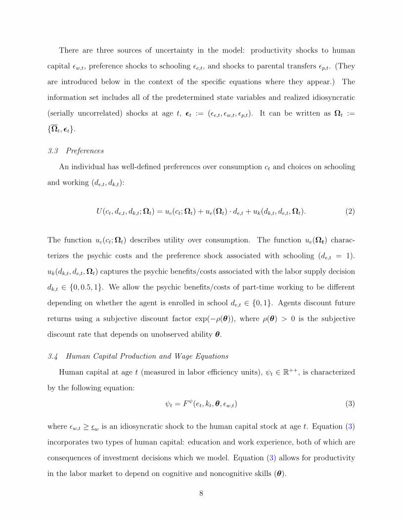
There are three sources of uncertainty in the model: productivity shocks to human

capital εw,t, preference shocks to schooling εe,t, and shocks to parental transfers εp,t. (They

are introduced below in the context of the specific equations where they appear.) The

information set includes all of the predetermined state variables and realized idiosyncratic

(serially uncorrelated) shocks at age t, εt := (εe,t, εw,t, εp,t). It can be written as Ωt :=

Ωt, εt.

3.3 Preferences

An individual has well-defined preferences over consumption ct and choices on schooling

and working (de,t, dk,t):

U(ct, de,t, dk,t; Ωt) = uc(ct; Ωt) + ue(Ωt) · de,t + uk(dk,t, de,t,Ωt). (2)

The function uc(ct; Ωt) describes utility over consumption. The function ue(Ωt) charac-

terizes the psychic costs and the preference shock associated with schooling (de,t = 1).

uk(dk,t, de,t,Ωt) captures the psychic benefits/costs associated with the labor supply decision

dk,t ∈ 0, 0.5, 1. We allow the psychic benefits/costs of part-time working to be different

depending on whether the agent is enrolled in school de,t ∈ 0, 1. Agents discount future

returns using a subjective discount factor exp(−ρ(θ)), where ρ(θ) > 0 is the subjective

discount rate that depends on unobserved ability θ.

3.4 Human Capital Production and Wage Equations

Human capital at age t (measured in labor efficiency units), ψt ∈ R++, is characterized

by the following equation:

ψt = Fψ(et, kt,θ, εw,t) (3)

where εw,t ≥ εw is an idiosyncratic shock to the human capital stock at age t. Equation (3)

incorporates two types of human capital: education and work experience, both of which are

consequences of investment decisions which we model. Equation (3) allows for productivity

in the labor market to depend on cognitive and noncognitive skills (θ).

8

An individual’s hourly wage offer depends on his human capital, whether he works part-

time or full-time, and whether the individual is enrolled in school:

wt = ψt · Fw(dk,t, de,t) (4)

where Fw(dk,t, de,t) is the market price per unit human capital. We allow the rental price

of human capital to be different between part-time jobs and full-time jobs. The part-time

wage may differ depending on whether the individual is enrolled in school (see Johnson,

2013). We normalize the market price of human capital for a full-time job to be unity (i.e.,

Fw(1, 0) = 1). Thus, an individual’s full-time wage offer equals to his human capital level:

wt = ψt = Fψ(et, kt,θ, εw,t) if dk,t = 1.

After leaving school, the accumulated years of work experience evolves via:

kt+1 = kt + 1(dk,t > 0)− δkkt1(dk,t = 0) := F k(kt, dk,t) (5)

where δk is the depreciation rate of work experience in each period when the individual does

not work. Education level at t+ 1, measured by years of schooling, evolves according to the

following relationship:

et+1 = et + de,t. (6)

3.5 Financial Market Frictions and Endogenous Credit Constraints

To finance education and consumption, individuals can borrow at a fixed interest rate

rb. Individuals can also accumulate physical assets at riskless rate rl.4 To capture an

important feature of imperfect capital markets, we allow the lending rate to be smaller than

the borrowing rate, i.e., rl < rb.5

The smallest amount of net worth st+1 that an agent can hold at the end of period t

4We abstract from portfolio choices.5We only need to keep track of an agent’s net worth. There is no need to separately keep track of an

agent’s debts and assets.

9

is captured by a (potentially negative) lower bound St+1 ∈ R−, which is determined by

both the private loan market borrowing limit and the maximum credit from the government

student loan programs as follows:

st+1 ≥ St+1 := −maxde,t · Lg(et + de,t), L

s

t(et+1, kt+1,θ) (7)

where Lg(et + de,t) ∈ R+ is the maximum government student loan credit for schooling level

(et + de,t) if the individuals choose to enroll in school (de,t = 1), and Ls

t(et+1, kt+1,θ) ∈ R+ is

the natural borrowing limit of an individual in the private debt market. Ls

t(et+1, kt+1,θ) is

determined by the maximum loan that the individual can pay back with probability one at

the end of his decision period T , i.e., Ls

T = 0. We discuss the formulation of the endogenous

natural borrowing limit Ls

t(·) in Section 3.8 below.

After leaving school, the borrowing limits St+1 are enforced in the following ways.6 Con-

sider two different situations. First, if an agent’s current debt level does not exceed his private

debt limit during previous period (i.e., st ≥ −Ls

t−1(et, kt,θ)), which could happen if the agent

did not borrow more than his private debt limit when in school or the agent (voluntarily)

paid down his previous student debt, his lower bound on net worth at the end of period t

is given by his private market natural borrowing limit (i.e. St+1 = −Lst(et+1, kt+1,θ)). By

construction, there will be no default in the model under such a situation.

Second, suppose that an agent’s current debt level exceeds his private debt limit during

the previous period (i.e., st < −Ls

t−1(et, kt,θ)). This can only happen if the agent borrows

from student loan programs. Since he is not forced to repay the debt, we reset the asset

lower bound St+1 equal to the agent’s current debt level (i.e. St+1 = st < 0) for t ≤ T − 1.

This is designed to capture the fact that students are not forced to repay their student

loans immediately. Student loans, in general, cannot be discharged through bankruptcy.7

Therefore, the model assumes that student debt will remain with the borrower until it is

6See Johnson (2013).7See Lochner and Monge-Naranjo (2015) for evidence supporting this assumption.

10

repaid. At the end of period T , the agent must pay back his student loans up to his available

resources. Any remaining unpaid student loans which the agent does not have resources to

pay, are forgiven.8 While in principle agents can plan to carry student debt through the end

of life and then default, doing so reduces their ability to borrow further over the lifetime to

smooth consumption.9

3.6 Budget Constraint and Transfer Functions

To finance a youth’s college tuition and fees, parents may provide financial transfers

trp,t ≥ 0. Parental financial transfers are generated by a stochastic function that depends

on (i) parents’ wealth terciles (sp) and parents’ education (ep); (ii) decisions about schooling

and employment (de,t, dk,t); (iii) youth’s cognitive ability and noncognitive ability (θ) and

current education (et) and age t. This is captured by:

trp,t = trp(ep, sp, de,t, dk,t,θ, et, t, εp,t) (8)

where εp,t is an idiosyncratic shock to parental transfers. Examples of parental monetary

transfers include college financial gifts if the youth chooses to attend college. The parental

transfer rule is determined outside our model. It captures paternalism and tied transfers on

the part of the parents, which is consistent with the findings of previous research (see, e.g.,

Keane and Wolpin, 2001 and Johnson, 2013).

Our parental transfer function allows for more heterogeneity in family transfers than

those used in Keane and Wolpin (2001) and Johnson (2013). In our parental transfer function

specification, even among the students who make the same schooling-working decisions, there

is heterogeneity in parental transfers due to differences in (1) parents’ net worth and parents’

education, which affect total available resources to the youth, (2) the youth’s own cognitive

8In the case of involuntary default at the end of period T , the agent will consume a minimum sustainableconsumption level cT = cmin > 0 and ST+1 = 0. We will discuss cmin in the next section (Section 3.6).

9Under the estimated model parameter values, our simulation shows that there is no default at the endof last period T among the simulated individuals.

11

ability and noncognitive ability, which affect the psychic and labor market monetary returns

of education, and (3) the shocks to the transfer function (ep,t).10

Defining r(st) := rl1(st > 0) + rb1(st < 0), the budget constraint for an individual who

chooses to attend college (i.e., de,t · 1(et + de,t ≥ 13) = 1) is:

ct + (tc(et + de,t)− gr(et + de,t, sp)) + st+1 = (1 + r(st)) · st + wt · h(dk,t) + trp,t (9)

ct ≥ rc(et + de,t) (10)

where tc(et + de,t) is the amount of college tuition and fees, gr(et + de,t, sp) is the amount of

grants and scholarships which depend on schooling level and parental wealth, and rc(et+de,t)

denotes the cost of college room and board. We require that the consumption expenditure

for those who choose to go to college must be no less than the cost of college room and

board.

The budget constraint for an individual who is not currently enrolled in college (i.e.,

de,t · 1(et + de,t ≥ 13) = 0) is:

ct + st+1 = (1 + r(st)) · st + wt · h(dk,t) + trp,t + trc,t + trg,t (11)

ct ≥ trc,t (12)

ct ≥ cmin (13)

where trc,t ≥ 0 is the direct consumption subsidy from the parents to their dependent child in

the forms of shared housing and meals.11 ct ≥ trc,t requires that trc,t only be a consumption

subsidy. It cannot be used by the youth to finance his college expenses or pay back his debt.

trg,t ≥ 0 is the amount of government transfers, which consist of unemployment benefits and

means-tested transfers that guarantee a minimum consumption floor cmin. Treating cmin as

10Park (2016) finds that the source of parental transfer heterogeneity depends on factors that affect thetotal resources available to youth, such as parental wealth and altruism, and on factors that affect themonetary or psychic returns to education.

11It is only received when the child is age 17 and is not attending college.

12

a subsistence level of consumption, we require ct ≥ cmin.

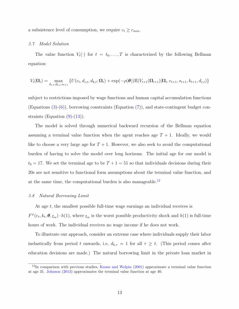
3.7 Model Solution

The value function Vt(·) for t = t0, . . . , T is characterized by the following Bellman

equation:

Vt(Ωt) = maxde,t,dk,t,st+1

U(ct, de,t, dk,t; Ωt) + exp(−ρ(θ))E(Vt+1(Ωt+1)|Ωt, et+1, st+1, kt+1, de,t)

subject to restrictions imposed by wage functions and human capital accumulation functions

(Equations (3)-(6)), borrowing constraints (Equation (7)), and state-contingent budget con-

straints (Equation (9)-(13)).

The model is solved through numerical backward recursion of the Bellman equation

assuming a terminal value function when the agent reaches age T + 1. Ideally, we would

like to choose a very large age for T + 1. However, we also seek to avoid the computational

burden of having to solve the model over long horizons. The initial age for our model is

t0 = 17. We set the terminal age to be T + 1 = 51 so that individuals decisions during their

20s are not sensitive to functional form assumptions about the terminal value function, and

at the same time, the computational burden is also manageable.12

3.8 Natural Borrowing Limit

At age t, the smallest possible full-time wage earnings an individual receives is

Fψ(et, kt,θ, εw) ·h(1), where εw is the worst possible productivity shock and h(1) is full-time

hours of work. The individual receives no wage income if he does not work.

To illustrate our approach, consider an extreme case where individuals supply their labor

inelastically from period t onwards, i.e, dk,τ = 1 for all τ ≥ t. (This period comes after

education decisions are made.) The natural borrowing limit in the private loan market in

12In comparison with previous studies, Keane and Wolpin (2001) approximate a terminal value functionat age 31. Johnson (2013) approximates the terminal value function at age 40.

13

period t− 1 in this extreme case is:

Ls

t−1(e, kt,θ) =Ls

t(e, kt + 1,θ) + max0, Fψ(e, kt,θ, εw) · h(1)− cmin1 + rb

.

When employment decisions are endogenous, the formulation of the natural borrowing

limit requires further thought. Let the credit limit at time t be Ls

t for an individual who

does not work at t. The natural borrowing limit at period t− 1 is (suppressing arguments)

Ls

t−1 = Ls

t/(1 + rb). This can be interpreted as saying that individuals borrow new loans at

time t, Ls

t , to pay back debt (1+rb)Ls

t−1. At age t the individual carries debt st+1 = −Lst ≤ 0

and consumes government transfers cut = trg,t ≥ cmin. Let Cevt be the compensation that

makes an individual indifferent between working and not working. We implicitly define Cevt

as the solution to the following indifference relationship:

uc(Cevt ; Ωt) + uk(dk,t = 1,Ωt) (14)

+ exp(−ρ(θ))E(Vt+1(Ωt+1)|Ωt, e, st+1 = −Lst(e, F k(kt, dk,t = 1),θ), kt+1 = F k(kt, dk,t = 1))

= uc(cut ; Ωt) + uk(dk,t = 0,Ωt)

+ exp(−ρ(θ))E(Vt+1(Ωt+1)|Ωt, e, st+1 = −Lst(e, F k(kt, dk,t = 0),θ), kt+1 = F k(kt, dk,t = 0)).

We require that the consumption compensation has to be at least equal to the subsistence

level. Thus, if Cevt < cmin, we set Cev

t = cmin.13 As seen in Equation (14), Cevt depends on

the individual’s psychic cost of working, and the future productivity gains of increased work

experience, government transfers (including unemployment benefits), and the sustainable

consumption level. In particular, the minimum consumption compensation Cevt is high if

(i) the individual’s psychic cost of working (−uk(dk,t = 1,Ωt) + uk(dk,t = 0,Ωt)) is high,

(ii) the returns to work experience (E(Vt+1(Ωt+1)|Ωt, e, st+1 = −Lst(e, F k(kt, dk,t = 1), kt+1 =

F k(kt, dk,t = 1))−E(Vt+1(Ωt+1)|Ωt, e, st+1 = −Lst(e, F k(kt, dk,t = 0), kt+1 = F k(kt, dk,t = 0)))

13In this case, given normality of goods, the first expression in (14) is bigger than the second expressionand the agent always works.

14

is low, and (iii) the government welfare subsidy (cut = trg,t) is high.

Equation (14) can be interpreted as an individual rationality constraint of working. The

individual chooses to work only if his consumption level under working is at least Cevt .

Under the most unfavorable possible income shocks, if wage earnings are higher than the

consumption equivalence value, i.e., Fψ(e, kt,θ, εw)·h(1) ≥ Cevt , the individual works dk,t = 1

and the maximum amount of debt that he can pay back at age t is

Fψ(e, kt,θ, εw) ·h(1)−Cevt . This is the surplus of employment in terms of consumption value

under the most unfavorable productivity shock. Using this notation, when an individual can

choose between full-time working and not working, the individual’s natural borrowing limit

is:

Ls

t−1(e, kt,θ) =Ls

t(e, kt+1,θ) + max0, Fψ(e, kt,θ, εw) · h(1)− Cevt (e, kt,θ)

1 + rb(15)

kt+1 = F k(kt, dk,t), dk,t = 1(Fψ(e, kt,θ, εw) · h(1)− Cevt (e, kt,θ) ≥ 0). (16)

It is straightforward to extend the previous derivation to take into account the part-time

employment choices (or any discrete employment choices). Specifically, we define the em-

ployment specific consumption compensation Cevt (dk,t; e, kt,θ) associated with employment

status dk,t as follows:

uc(Cevt (dk,t; e, kt,θ); Ωt) + uk(dk,t,Ωt) (17)

+ exp(−ρ(θ))E(Vt+1(Ωt+1)|Ωt, e, st+1 = −Lst(e, F k(kt, dk,t),θ), kt+1 = F k(kt, dk,t))

= uc(cut ; Ωt) + uk(0,Ωt)

+ exp(−ρ(θ))E(Vt+1(Ωt+1)|Ωt, e, st+1 = −Lst(e, F k(kt, 0),θ), kt+1 = F k(kt, 0)).

Note that when dk,t = 0, Cevt (dk,t = 0; e, kt,θ) = cut > 0 satisfying Equation (17) automati-

cally.

15

Thus, the endogenous borrowing limit as defined in this paper is:

Ls

t−1(e, kt,θ) =Ls

t(e, kt+1,θ) + max0, [Fψ(e, kt,θ, εw)Fw(dk,t, 0) · h(dk,t)− Cevt (dk,t; e, kt,θ)]

1 + rb

(18)

dk,t = arg maxdk,t∈0,0.5,11(dk,t > 0)

(Fψ(e, kt,θ, εw)Fw(dk,t, 0) · h(dk,t)− Cev

t (dk,t; e, kt,θ))

(19)

kt+1 = F k(kt, dk,t). (20)

Equations (18) and (20) imply that if(Fψ(e, kt,θ, εw)Fw(dk,t, 0) · h(dk,t)− Cev

t (dk,t; e, kt,θ))<

0 for dk,t > 0, then dk,t = 0, Ls

t−1(e, kt,θ) = Lst (e,kt+1,θ)

1+rb, and kt+1 = F k(kt, 0).

At terminal age T , LT (·) = 0, we calculate CevT (·) using Equation (17). We then calculate

the natural borrowing limit LT−1(·) at T−1 based on Equations (18) to (20). Using Equations

(17)-(20), we calculate the natural borrowing limit recursively at any age.

The natural borrowing limit derived in our model implies that at a given age, an in-

dividual’s borrowing limit is lower if (i) the individual has a low level of human capital,

(ii) the individual’s psychic cost of working is higher, (iii) the returns to work experience

are lower, and (iv) the government welfare subsidy for not working is higher. An agent’s

human capital affects his borrowing limit by affecting his future earning capacity Fψt (·)t.

The individual’s psychic cost of working, the future productivity gains of increased work

experience, and government welfare policy affect borrowing limits by affecting the minimum

consumption compensation level Cevt .

3.9 Discussion of the Natural Borrowing Limit

The concept of the natural borrowing limit was first proposed in Aiyagari (1994).14 He

defines the natural borrowing limit as the maximum amount an individual can repay with

certainty. The underlying regime that would generate this constraint is one in which lenders

14Huggett (1993) develops a model with incomplete-insurance where agents faces a borrowing constraintof one year’s income.

16

can fully enforce contracts and collect on all resources available to the individual.15

Our notion of the natural borrowing limit extends Aiyagari’s borrowing limit by consid-

ering endogenous labor supply and human capital investment. Following Aiyagari (1994), we

assume that lenders can fully enforce contracts and can collect from all resources available to

the individual. Borrowers must repay as long as they have resources. However, different from

Aiyagari, who assumes that earnings are exogenous, in our model labor supply is endoge-

nous and lenders cannot force borrowers to work. Since borrowers always have the choice

not to work and collect welfare covering their minimum consumption requirement, lenders

can never drive borrower’s utility below that value or they will collect nothing. Hence, the

lending regime with endogenous labor supply is that lenders can enforce full repayment sub-

ject to the restriction that borrowers must be provided a minimum consumption level (Cevt

defined by Equation (17)) that satisfies the borrower’s individual rationality constraint of

working.

Our formulation of the borrowing limit, that takes into account individual decisions about

labor supply and human capital accumulation, is related to studies that assume imperfectly

enforceable contracts (see Marcet and Marimon (1992), Kehoe and Levine (1993), Albu-

querque and Hopenhayn (2004), and Cooley et al. (2004), Cagetti and De Nardi (2006)).

Imperfect enforceability of contracts means that the creditors are not able to force the debtors

to fully repay their debts as promised and that the debtors fully repay only if it is in their own

interest to do so. Since both parties are aware of this feature and act rationally, the lender

will lend to a given borrower only an amount (possibly zero) that will be in the debtor’s

interest to repay as promised.

Our natural borrowing limit does not depend on parental transfers. In our model, parental

financial transfers trp,t are governed by a stochastic transfer rule. The lowest possible value

of parental financial transfers (regardless of the youth’s choices) is zero, which consequently

implies that the youths cannot credibly promise to pay back positive loans using (possibly

15It is one motive for precautionary saving (see Zeldes, 1989).

17

zero) parental transfers with certainty. Parental consumption transfer trc,t is in the form

of shared housing and meals provided by their parents. Youth cannot “cash” such con-

sumption subsidy to pay back their debt. Regarding government transfers, we assume that

private lenders cannot touch government transfers including tuition subsidies and grants.

Hence the formation of the natural borrowing limit does not take into account government

transfers. However, both parental and governmental transfers affect labor supply decisions

and accumulated work experience, and hence indirectly affect the natural borrowing limit.

We implicitly assume that borrowers can costlessly signal their private information to

lenders so that there is no asymmetric information in the lending market. Examples of such

signals include past history of wage earnings, employment, criminal background, test scores

on cognitive ability, and FICO scores, etc. Any restrictions that reduce an individual’s ability

to signal his own type will result in asymmetric information in the lending market and may

reduce the amount of the borrowing limits for the most able individuals.16

Our analysis differs from Navarro and Zhou (2016), who estimate a model with a ver-

sion of an Aiyagari borrowing constraint.17 They assume, in our notation, that Ls

t(e) =

Y MINT+1 (e)/(1 + rb)

T+1−t, where Y MINT+1 (e) > 0 is the social security income after retirement

that depends on education. They assume that agents always work a minimum number of

hours. They do not account for individual rationality constraints of working in their for-

mulation of borrowing limits. The decision to work does not affect private debt limits.

They do not allow for post-schooling human capital accumulation nor do they account for

16Our extension of the Aiyagari credit constraint does not capture the full array of credit market possibili-ties facing agents. They may go bankrupt with varying penalties ranging from full market exclusion (Alvarezand Jermann, 2001) to a range of other possible penalties (Chatterjee et al., 2007). Lenders can monitorand adjust period-by-period loans based on employment and medical histories, and other events realized byagents (see Chatterjee et al., 2007 and Jermann and Quadrini, 2012). A variety of financial arrangementsare available to lenders and borrowers (see Gertler and Kiyotaki, 2010). Lenders can monitor borrowers anddemand collateral or some form of enforceable partial repayment conditions. The assumption that the onlybinding constraint facing agents is that they must repay debt in the terminal period (up to some limit) issurely an extreme simplification of a richer set of period-by-period market and default opportunities. More-over, it assumes some implicit mechanism through which agents comply with a no-terminal-default rule. Wethank Dean Corbae, Jorge Garcıa, and Lars Hansen for stimulating conversations on these issues.

17Terminal assets must be no less than a particular lower bound.

18

access to student loans, heterogeneity in parental transfers, and heterogeneity in parental

characteristics.

In contrast, our formulation of the borrowing limit extends Aiyagari’s borrowing limit into

the realm of imperfectly enforceable contracts where agents’ decision to work, the psychic

cost of working, unobserved ability, and endogenous human capital accumulation (both in

terms of education and work experience) directly affect the private debt limit.

Our analysis differs from the approaches of Keane and Wolpin (2001) and Johnson (2013)

by not introducing additional free parameters from outside the model to proxy unmeasured

credit constraints. Ours is a far more stringent approach to estimation. Finally, unlike other

approaches in the literature, we do not specify ad hoc fixed credit limits (see, for example,

Abbott et al., 2016) or calibrate the model to fit asset distributions. Table 1 summarizes

how the literature models credit constraints and our distinct approach to modeling them.

3.10 Optimal Decisions

The envelope condition is:

∂Vt∂st

= λb,t(1 + r(st)), if st 6= 0, (21)

where r(st) = rl1(st > 0) + rb1(st < 0) and λb,t is the Lagrange multiplier associated with

the budget constraint.

The first-order conditions with respect to ct > 0 and st+1 6= 0, t < T are:

∂uc(ct; Ωt)

∂ct= λb,t (22)

exp(−ρ(θ))

(∂EVt+1

∂st+1

)+ λs,t = λb,t (23)

where λs,t is the Kuhn-Tucker multiplier of the borrowing constraint. If λs,t > 0, the bor-

rowing constraint binds, i.e., st+1 = St+1. If λs,t = 0, the borrowing constraint does not bind

and the individual is able to smooth consumption between ages t and t+ 1.

19

Individuals value education and work experience not only because they improve produc-

tivity and earnings, but because they increase the natural borrowing limit and thus provide

insurance values for consumption against adverse wage shocks. The first order conditions

are consistent with agent rationality associated with the employment choices.

3.11 Initial Conditions and Our Measurement System

We complete the specification of our model by defining initial conditions and a set of

measurement equations that relate proxied cognitive and noncognitive endowments to a set

of observed measures. Individuals start life as autonomous agents at age 17 (t0 = 17). The

age 17 information set, Ω17, is:

Ω17 := (17, θc, θn, k17, e17, s17, de,16, ep, sp).

The initial condition at age 17 that can be determined from sample information are:18

Ωobserved

17 := (17, k17, e17, s17, de,16, ep, sp).

We proxy θ but do not directly observe it.

The joint distribution of unobserved ability at initial age 17, conditional on parental

background at 17 (X17) is given by:

θcθn

X17 ∼ N

µc(ep, sp)µn(ep, sp)

,

σ2c σc,n

σc,n σ2n

where µj(ep, sp) = µj + µj,e,11(ep = 12) + µj,e,21(ep > 12 & ep < 16) + µj,e,31(ep ≥ 16) +

µj,s,11(sp = 2nd Tercile) + µj,s,21(sp = 3rd Tercile), for j = c, n. Thus we allow the initial

distribution to differ by parents’ wealth and education to capture early parental investment

18Education, lagged school attendance, parental education, and parental wealth (e17, de,16, ep, sp) are ob-served in our sample. We also set the accumulated years of working experience and net worth at age 17 tobe zero (k17 = 0, s17 = 0).

20

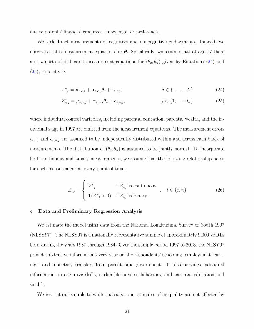
due to parents’ financial resources, knowledge, or preferences.

We lack direct measurements of cognitive and noncognitive endowments. Instead, we

observe a set of measurement equations for θ. Specifically, we assume that at age 17 there

are two sets of dedicated measurement equations for (θc, θn) given by Equations (24) and

(25), respectively

Z∗c,j = µz,c,j + αz,c,jθc + εz,c,j, j ∈ 1, . . . , Jc (24)

Z∗n,j = µz,n,j + αz,n,jθn + εz,n,j, j ∈ 1, . . . , Jn (25)

where individual control variables, including parental education, parental wealth, and the in-

dividual’s age in 1997 are omitted from the measurement equations. The measurement errors

εz,c,j and εz,n,j are assumed to be independently distributed within and across each block of

measurements. The distribution of (θc, θn) is assumed to be jointly normal. To incorporate

both continuous and binary measurements, we assume that the following relationship holds

for each measurement at every point of time:

Zi,j =

Z∗i,j if Zi,j is continuous

1(Z∗i,j > 0) if Zi,j is binary., i ∈ c, n (26)

4 Data and Preliminary Regression Analysis

We estimate the model using data from the National Longitudinal Survey of Youth 1997

(NLSY97). The NLSY97 is a nationally representative sample of approximately 9,000 youths

born during the years 1980 through 1984. Over the sample period 1997 to 2013, the NLSY97

provides extensive information every year on the respondents’ schooling, employment, earn-

ings, and monetary transfers from parents and government. It also provides individual

information on cognitive skills, earlier-life adverse behaviors, and parental education and

wealth.

We restrict our sample to white males, so our estimates of inequality are not affected by

21

issues of race or gender. We use the unweighted data.19 Our final sample contains 2,102

individuals, with 25,639 individual-year observations. Table A1 in the Web Appendix reports

the number of observations dropped in each step of our sample selection.

4.1 Variable Description

Measures of Cognitive Ability and Noncognitive Ability

We use the Armed Services Vocational Aptitude Battery (ASVAB) scores as measures of

cognitive ability.20 Specifically, we consider the scores from Mathematical Knowledge (MK),

Arithmetic Reasoning (AR), Word Knowledge (WK), and Paragraph Comprehension (PC).

These four scores have been used by NLSY staff to create the Armed Forces Qualification

Test (AFQT) score, which is commonly used in the literature as a measure of IQ or cognitive

ability. ASVAB scores are only asked in the year 1999.

Our measures of noncognitive ability include three variables that indicate respondents’

adverse behaviors at very early ages. Specifically, we use violent behavior in 1997 (have ever

attacked anyone with the intention of hurting or fighting), theft behavior in 1997 (have ever

stolen something worth $50 or more), and any sexual intercourse before age 15. Individuals

with high noncognitive ability are less likely to display adverse behaviors. (See Heckman

and Kautz, 2014 and Kautz and Zanoni, 2015 for discussions of these measures and their

validity.)

Education and Labor Market Outcomes

Education is measured by the highest grade completed. We manually recode this variable

by cross-checking the highest grade completed with data on enrollment and the highest degree

received, in order to correct for missing data, data coding errors, and GEDs. In particular, a

high school dropout with a GED is recoded to his highest grade of school actually completed.

19See Johnson (2013) for the same procedure.20The CAT-ASVAB is an automated computerized test developed by the United States Military which

measures overall aptitude. The test is composed of 12 subsections and has been well-researched for its abilityto accurately capture the aptitude of test-takers.

22

The NLSY97 records the number of hours worked in each week, the number of weeks

worked in a year, and total income earned in a year. We define full-time working to be

working no less than 30 hours a week, and part-time working to be working less than 30

hours a week but more than or equal to 10 hours a week. Among workers aged 23 and above,

the average full-time employment annual hours of work is 2,314 and the median is 2,184,

and the average part-time annual hours of work is 998 and the median is 1,040. Frequency

distributions of weeks and hours worked are provided in the Web Appendix Figure A1. For

employed workers, the hourly wage rate is the ratio between total earned income and total

actual hours worked (in 2004 dollars).

The NLSY97 collects detailed information on assets and debts of respondents at ages

20, 25, and 30. We define net worth as all assets (including housing assets and all financial

assets) minus all debt (including mortgages and all other debts).21

Parental Education, Net Worth, and Transfers

The NLSY97 asks each respondent about their parents’ schooling and net worth informa-

tion only in round 1 (1997). We define parents’ education as the average years of schooling

of father and mother if both the father’s and mother’s schooling are available.22 For single-

parent families where only one parent’s schooling level is available, we define the parents’

schooling only using the single parent’s schooling level. Parents’ net worth is defined as all

assets (including housing assets and all financial assets) minus all debt (including mortgages

and all other debts). Parental transfer data is constructed as total monetary transfers re-

ceived from parents in each year, including allowance, non-allowance income, college financial

21In our sample, the bottom 1% of net worth is -$42,028 and the bottom 5% is -$6,604. The net worth isskewed to the right, the median net worth is $8,504, the top 10% of the net worth is $80,630, and the top5% is $146,364. We bottom-code the net worth to be -$75,000 and top-code the net worth to be $100,000.In Johnson (2013), asset values are top coded at $45,000 and bottom coded at -$35,000 for NLSY97 malesaged 18 to 26.

22We top-code parents years of schooling to be 16 years (4-year college graduate) and bottom code parentsschooling to be 8 years (high school dropouts).

23

aid gift, and inheritance.23

4.2 Summary Statistics

Table 2: Key Variables over Age

Age 17 Age 20 Age 25 Age 30In School 0.87 0.37 0.10 0.01Full-Time Working 0.04 0.44 0.73 0.78Part-Time Working 0.49 0.30 0.12 0.06Part-Time Working While in School 0.46 0.24 0.07 0.03Education 10.34 12.25 13.43 13.78Years Worked 0.00 0.77 3.92 8.05Net Worth 0.00 13467.81 20569.12 34826.70Full-Time Hourly Wage 6.10 9.55 14.71 18.25Part-Time Hourly Wage 6.16 8.46 15.28 15.77Receive Parental Transfers 0.37 0.46 0.18 0.06Total Parental Transfers 428.53 1766.64 315.89 83.51

Table 3: Measures of Cognitive and Noncognitive Ability (Year 1997)

mean sd min max NASVAB: Arithmetic Reasoning (1997) -0.08 0.95 -3.14 2.37 1,786ASVAB: Mathematics Knowledge (1997) 0.06 0.98 -2.80 2.68 1,781ASVAB: Paragraph Comprehension (1997) -0.16 0.93 -2.36 1.83 1,784ASVAB: Word Knowledge (1997) -0.28 0.89 -3.15 2.35 1,785Noncognitive: Violent Behavior (1997) 0.22 0.42 0.00 1.00 2,097Noncognitive: Had Sex Before Age 15 0.18 0.38 0.00 1.00 2,100Noncognitive: Theft Behavior (1997) 0.10 0.30 0.00 1.00 2,098

23College financial aid gift includes any financial aid respondents received from relatives and friends thatare not expected to be paid back for each college and term attended in each school year.

24

Figure 1: Parental Monetary Transfers By Parental Characteristics

050

01,

000

1,50

02,

000

Pare

ntal

Tra

nsfe

rs

Parents' Net Worth T1 Parents' Net Worth T2 Parents' Net Worth T3

Parents' educ < 12 yrs Parents' educ = 12 yrs Parents' educ 13 to 15 yrs Parents' educ >= 16 yrs

(a) By Parents’ Net Worth Terciles & Education

050

01,

000

1,50

02,

000

Pare

ntal

Tra

nsfe

rs

17 18 19 20 21 22 23 24 25 26 27 28 29 30 31Age

(b) By Youth’s Age

Source: NLSY97. Parental transfer is the total monetary transfers received from parents ineach year, including allowance, non-allowance income, college financial aid gift, andinheritance.

Table 2 reports the statistics of key variables by age.24 At age 17, 87% of the youth are

enrolled in school, and the fraction of the youth in school decreases to 10% at age 25. The

fraction of the youth who work full time steadily increases from 44% at age 20 to 78% at

age 30; the fraction of part-time employment decreases from 30% at age 20 to 6% at age

30. Average years of schooling increase from 10.3 at age 17 to 13.8 at age 30. The average

net worth increases from $13,468 at age 20 to $34,827 at age 30. Average hourly wages

(both part-time job and full-time job) increase between age 17 and age 30. Average full-time

hourly wage rate is $18 at age 30. All the variables are measured in 2004 dollars. Table A3

reports average years of work experience, wages, and net worth for 4 education groups at

age 25. Measures of cognitive and noncognitive skills at age 17 are presented in Table 3.

24The summary statistics for the entire sample over year 1997 to 2011 is reported in Table A2.

25

Figure 2: Relationships Between Early Endowments and Environments and College Choices

0.1

.2.3

.4.5

.6.7

.8.9

1 C

olle

ge A

ttend

ance

Rat

e

ASVAB Quartile 1 ASVAB Quartile 2 ASVAB Quartile 3 ASVAB Quartile 4

Parents' Schooling < 12 yrs Parents' Schooling = 12 yrs

Parents' Schooling 13 to 15 yrs Parents' Schooling >= 16 yrs

(a) College Attendance by Parental Education

0.1

.2.3

.4.5

.6.7

.8.9

1 C

olle

ge A

ttend

ance

Rat

e

ASVAB Quartile 1 ASVAB Quartile 2 ASVAB Quartile 3 ASVAB Quartile 4

Parents' Net Worth Tercile 1 Parents' Net Worth Tercile 2

Parents' Net Worth Tercile 3

(b) College Attendance by Parental Net Worth

0.1

.2.3

.4.5

.6.7

.8.9

1 4

-Yr C

olle

ge G

radu

atio

n R

ate

ASVAB Quartile 1 ASVAB Quartile 2 ASVAB Quartile 3 ASVAB Quartile 4

Parents' Schooling < 12 yrs Parents' Schooling = 12 yrs

Parents' Schooling 13 to 15 yrs Parents' Schooling >= 16 yrs

(c) 4-Year College Grad. by Parental Education

0.1

.2.3

.4.5

.6.7

.8.9

1 4

-Yr C

olle

ge G

radu

atio

n R

ate

ASVAB Quartile 1 ASVAB Quartile 2 ASVAB Quartile 3 ASVAB Quartile 4

Parents' Net Worth Tercile 1 Parents' Net Worth Tercile 2

Parents' Net Worth Tercile 3

(d) 4-Year College Grad. by Parental Net Worth

Source: NLSY97 white males. 4-Year college graduate rate is calculate as the fraction ofindividual whose years of schooling are more than or equal to 16 at age 25.

The distribution of parental transfers is skewed.25 The amount of parental transfers

to children is either positive or zero. On average, 29% of the youths receive zero monetary

transfers from their parents. Among those who receive positive parental transfers, the average

amount of transfers received is $3,116, and the median amount is $907. As shown in Figure

1, on average, the amount of parental transfers depends crucially on parental education and

net worth and varies over the youth’s life cycle.

25Conditional on parental transfers being positive, the top 1 percentile of the parental transfers amountis $24,639. We top-code the maximum amount of positive parental transfers to be $30,000 per year.

26

There is a positive impact of parental education and wealth on educational decisions.

As seen in Figure 2, even after controlling for measures of the youths’ own cognitive ability,

there is still a strong positive correlation between parents’ education and net worth and

an individual’s college attendance and 4-year college completion. Table 4 reports the OLS

regression results of years of schooling at age 30 on ASVAB, the number of early adverse be-

haviors, parental education, and parental net worth. After controlling for the ASVAB score,

individuals’ years of schooling are still positively correlated with both parental education

and parental net worth. Furthermore, college attendance decisions are negatively correlated

with the number of early adverse behaviors, which suggests a positive correlation between

years of schooling and noncognitive ability.26

Table 4: OLS Regression of Adult Educational Outcomes on Early Endowment and Family Influence

EducationASVAB 1.03∗∗∗ (0.03)Num of Adverse Behaviors -0.60∗∗∗ (0.04)Parents’ Education 0.27∗∗∗ (0.02)Parents’ Net Worth 2nd Tercile 0.67∗∗∗ (0.07)Parents’ Net Worth 3rd Tercile 1.12∗∗∗ (0.07)Age 0.09∗∗∗ (0.02)R2 0.46Observations 5354

Standard errors in parentheses.Source: NLSY97 white males aged 25 to 30.∗ p < 0.10, ∗∗ p < 0.05, ∗∗∗ p < 0.01

5 Empirical Strategy

The precise specifications used to estimate our model are reported in Section 5.1.27 In

Section 5.2, we discuss calibration of parameters that are identified using externally supplied

data. After that, we turn to consider model identification (Section 5.3) and estimation

(Section 5.4).

26Table A4 reports the OLS estimation results for logarithm of hourly wages among individuals who alwayswork after leaving school upon completing the highest degree.

27Web Appendix Section A.2 gives the parameterization of the parental transfer function.

27

5.1 Model Parameterization

We use the following additively separable current flow utility function:

U(ct, de,t, dk,t; Ωt) =(ct/est,e)

1−γ − 1

1− γ+ ue(Ωt)de,t + uk(dk,t, de,t,Ωt) (27)

where est,e is the equivalence scales of family size,28 ue(Ωt) and uk(dk,t, de,t,Ωt) are flow

utility (or disutility if negative) associated with individual choices of schooling and working,

respectively:

ue(Ωt) = φe,01(de,t + et ≤ 12) + (φe,1 + φe,a1(t > 22)) · 1(de,t + et > 12 & de,t + et ≤ 16)

+ φe,21(de,t + et > 16) + αe,cθc + αe,nθn + φe,p1(ep ≥ 16)− φe,e(1− de,t−1) + σeεe,t (28)

uk(dk,t, de,t,Ωt) = [φk,e · 1(dk,t = 0.5 & de,t = 1) + φk,0 · 1(dk,t = 0.5 & de,t = 0)

+ (φk,1 + φk,2(age− 17)) · 1(dk,t = 1)] · (1 + αk,cθc + αk,nθn) (29)

where the schooling preference shock εe,t is i.i.d. standard normal distributed.

We allow for the psychic costs of schooling to depend on an individual’s cognitive and

noncognitive abilities. φe,0, φe,1, and φe,2 characterizes the level of psychic costs for attend-

ing high school, college, and graduate school, respectively. φe,a is the psychic cost of late

enrollment in college, and φe,e is the psychic cost of re-entering school. We also introduce

preference heterogeneity in schooling depending on parental education level ep to allow for

the direct impact of parental education on schooling (φe,p). We allow for preference shocks

to the utility of schooling (εe,t).

Parameters φk,e, φk,0, and φk,1 govern the level of psychic costs of part-time working

while in school, part-time working while not in school, and full-time working, respectively.

28Household equivalence scales measure the change in consumption expenditures needed to keep the welfareof a family constant when its size varies. We calculate the equivalence scales of different household sizesfollowing Fernandez-Villaverde and Krueger (2007). For example, this scale implies that a household of twoneeds 1.34 times the consumption expenditure of a single household. We do not model endogenous changesin family size. Instead we allow family size to vary exogenously depending on education level e and age t.The average family size for each education group at every age is obtained from CPS data 1997 to 2012.

28

We allow the preference of full-time working to vary with age (φk,2). We also allow the

psychic costs of working to depend on an individual’s cognitive and noncognitive abilities.

Following Gourinchas and Parker (2002) and De Nardi (2004), we assume that the ter-

minal value function at age T + 1 takes the following functional form:

VT+1(ΩT+1) = φs(sT+1/esT,e)

1−γ − 1

1− γ, (30)

where φs characterizes the influence of net worth at age T + 1. Equation (30) approximates

an individual’s value function at age T + 1. It does not imply that individuals die at age

T + 1 or that other state variables in ΩT+1 do not matter. It just implies that the marginal

effects of other state variables (such as accumulation of education and experience) on the

individual’s value function at age T+1 are small. As noted in Section 3.7, we set the terminal

age to be T + 1 = 51.

We allow the subjective discount rate ρ(θc, θn) to depend on cognitive ability and noncog-

nitive ability:

ρ(θc, θn) = ρ0(1− ρcθc − ρnθn) (31)

An individual’s wage function and human capital function are characterized by:

logwt = logψt + 1(dk,t = 0.5)(βw,0 + βw,1de,t) (32)

where

logψt =βψ,0 + βψ,kkt + βψ,kkk2t /100 + βψ,e,0(et − 12)

+ βw,e,11(et = 12) + βw,e,21(et > 12 & et < 16) + βw,e,31(et ≥ 16)

+ (αψ,c,0θc + αψ,n,0θn) · 1(et < 12)

+ (αψ,c,1θc + αψ,n,1θn) · 1(et ≥ 12 & et < 16)

+ (αψ,c,2θc + αψ,n,2θn) · 1(et ≥ 16) + εw,t − E(εw,t)

where εw,t is the education specific idiosyncratic productivity shock. We allow the density

29

function of εw,t to differ depending on whether the individual has a four-year college degree

or not.

Without loss of generality, we normalize the lowest possible value of εw,t to be 0: εw = 0.

We assume that the productivity shock εw,t ≥ εw = 0 is drawn from a gamma distribution

Gamma(a, b) with the following density function:

p(εw,t) =1

Γ(a)ba(εw,t)

a−1e−(εw,t)/b. (33)

Therefore, E(εw,t) = ab and V ar(εw,t) = ab2. The gamma distribution allows us to flexibly

model both the shape and the scale of the productivity shock distribution which are governed

by the parameters a and b, respectively.29

5.2 External Calibration

For parameters that can be identified outside the structural model, such as the mone-

tary cost of schooling and government transfers, we rely on external data sources. Table 5

summarizes all the parameters that are externally specified in our structural model. We now

discuss these choices in detail.

We calculate the cost of college tuition and fees and grants and scholarships from the

following two sources: (i) Total direct expenditures (including tuition and fees) of higher

education level et are calculated as the average expenditures per student using data from

The Integrated Postsecondary Education Data System (IPEDS); (ii) The average amount of

the grant for each education level associated with every parental net worth tercile using the

NLSY97 sample. We also obtain the average cost of college room and board from IPEDS

for two-year college and 4-year college, respectively.

We set the borrowing interest rate equal to 5 percent annually. We set the lending

interest rate rl to be 1 percent annually, which is the average real interest rate on 1-year

29Chatterjee et al. (2007) assume that the distribution function of εw,t is characterized by a one-parameter

distribution function: Prob(εw ≤ z) =(z−εwεw−εw

)φw

, where φw controls the shape of the shock distribution

and εw is the upper bound of the shock. Our specification is more flexible.

30

Table 5: Parameters Calibrated Outside the Structural Model

Description Parameter Value Source

College Tuition & Feestc(e = 13, 14) $5,073 IPEDS data on average tuition and fees

1999-2006.tc(e ≥ 15) $10,653

College Grants andScholarship

gr(e = 13, 14, sp = T1) $2,581

NLSY97 data on average grants andscholarship by years of schooling andparental wealth terciles.

gr(e = 13, 14, sp = T2) $2,287gr(e = 13, 14, sp = T3) $2,476gr(e ≥ 15, sp = T1) $3,604gr(e ≥ 15, sp = T2) $2,569gr(e ≥ 15, sp = T3) $2,607

College Room and Board rc(e = 13, 14) $4,539 Johnson (2013) room and board for 2-yearcollege and 4-year collegerc(e ≥ 15) $6,532

GSL Borrowing AnnualLimit

lg(e = 13) $2,625

Annual Stafford Loan Limits 1993 to 2007lg(e = 14) $3,500lg(e = 15, 16) $5,500lg(e > 16) $10,500

GSL Borrowing AggregateLimit

Lg(e ≥ 13 & e ≤ 16) $23,000 Undergraduate

Lg(e ≥ 16) $138,500 Graduate + Undergraduate

Borrowing Interest Rate rb 5% Federal Student AidLending Interest Rate rl 1% Average real interest rate on 1-year

U.S. government bonds from 2001 to2007

Parental TransferFunction

trp(ep, sp, de,t, dk,t, et, t) TableA5

NLSY97 sample

Parents ConsumptionSubsidy

trc,t = χ · 1(t < 18) $7,800 Kaplan (2012) & Johnson (2013)

Part-time Annual Hours h(0.5) 1,040 20 hours per week, 52 weeksFull-time Annual Hours h(1) 2,080 40 hours per week, 52 weeks

Unemployment Benefitbg(e ≤ 12) $540× 3bg(e ≥ 13 & e ≤ 16) $600× 3 NLSY97 UI benefitsbg(e > 16) $740× 3

Minimum ConsumptionFloor

cmin $2,800 NLSY sample average means-testedtransfers among recipients

Risk Aversion Coefficient γ 2.0 Lochner and Monge-Naranjo (2012)and Johnson (2013)

Terminal Value function φs 25.0 PSID 1999-2011: Median(s51/c50)=5

IPEDS = Integrated Postsecondary Education Data System. Average tuition and fees are weighted by full-time enrollment and are deflated in 2004 dollars. Because expenditures are higher at four-year institutionsthan at two-year institutions, there is a noticeable jump in cost between two and three years of college.Within our sample period, the aggregate subsidized Stafford Loan Limits is $23,000 for undergraduate and$138,500 for graduate and undergraduate in total. The Interest rate ranges from 3.34 to 8.25% for StaffordLoans over the time period 1997 to 2011. Parental consumption subsidy is given by trc,t = χ · 1(t < 18),where χ is the value of direct consumption subsidy provided by the parents such as shared housing and mealswhen the youth attends high school.

31

U.S. government bonds from 2001 to 2007. Note that the interest rate spread on borrowing

and lending (4%) is quite large and already embodies an important market friction.

We estimate the logarithm of parental monetary transfers, log(trp,t+1) using our NLSY97

sample (see Section A.2 in the Web Appendix for parameterization); the parameter estimates

are reported in Web Appendix Table A5. In the sample, 94% of youth who are attending

high school live with their parents.30 Following Kaplan (2012) and Johnson (2013), we set

the consumption subsidy provided by parents for those who are living with their parents and

not attending school, χ, to be $650 monthly ($7,800 annually)31; χ includes both the direct

and indirect costs of housing as well as shared meals.

We set the hours of work to be 20 hours per week for part-time jobs and 40 hours per

week for full-time jobs (see Keane and Wolpin (2001)), therefore the annual hours of work

is 1,040 hours for part-time job and 2,080 hours for full-time job.32 We set the monthly

unemployment benefits to be $540 for unemployed workers without a college degree, $600

for some college or 4-year college workers, and $740 for workers with a graduate degree.33 We

assume that unemployed workers can receive unemployment benefits for 3 months. In our

sample, the average amount of means-tested transfers (including food stamps, AFDC and

WIC) among recipients is about $2,800 annually. Thus, we set the government means-tested

minimum consumption floor cmin to be $2,800.

We set the relative risk aversion parameter to be γ = 2.0 following Lochner and Monge-

Naranjo (2011) and Johnson (2013). A majority of existing microstudies on consumption

and savings estimate the value of γ to be between one and three.34

30The ratio is 42% for those who are not attending high school.31Our model abstracts away from multiple child households.32In our sample, among workers aged 23 and above, the median annual working hours of a part-time

worker is 1,040 and the median annual working hours of a full-time employed worker is 2,184.33Conditional on receiving unemployment benefits, the mean monthly unemployment insurance benefits

are $800 for workers with at most a high school degree, $900 for workers with some college or 4-year college,and $1,100 for workers with a graduate degree. In the model, we assume individuals who are not working or inschool receive unemployment benefits, which are substantially more generous than the actual unemploymentbenefits; we thus reduce the predicted unemployment benefits amount by one-third following Kaplan (2012).

34See Browning et al. (1999) for a summary of the early literature.

32

To calibrate the parameter in the terminal value function, we note that the first-order

optimal condition at age T can be written as cT−γ = φssT+1

−γ. From the Panel Study of

Income Dynamics (PSID) 1999 to 2011 the median value of sT+1

cTis 5.0 among households

whose head aged T + 1 = 51,35 therefore we set φs =(sT+1

cT

)γ= (5.0)γ = 25.0.

5.3 Identification

This section discusses identification of key features of the model.

5.3.1 Factor Model and Measurement System

The identification of factor models requires normalizations that set the location and scale

of the factors (see Anderson and Rubin (1956)). For each factor (θc, θn), we normalize its

unconditional mean to be zero, i.e., Eep,sp(θc), E(θc) = E(θn) = 0, and standard deviation

to be one, i.e., σc = σn = 1. We allow intercepts in all measurement equations.

5.3.2 Dynamic Model and Structural Parameters

This section provides an overview of identification of the structural model. The parame-

ters that remain to be identified are: 15 parameters characterizing individual preferences over

schooling and working, 20 parameters characterizing the human capital production function

(including the density function of productivity shocks) and wage function, and 3 parameters

regarding discount factors.

The parameters on the subjective discount rate can in principle be identified by using

consumption data formed from the asset data. To illustrate, consider the Euler equation

under a CRRA utility specification for those who are far away from borrowing constraints

(abstracting from uncertainty):36

γ · (log ct+1 − log ct) = −ρ(θc, θn) + log(1 + r),

35To be consistent with our net worth measure in the data section, we also measure net worth as all assets(including housing assets and all financial assets) minus all debts (including mortgages and all other debts)in PSID.

36For illustrative purposes, here we assume uc(ct; Ωt) = c1−γt /1− γ and r is the borrowing/lending interestrate.

33

using the fact that γ is set externally.37 The identification of the parameters of the subjective

discount rate function ρ relies on variations in consumption growth and thus savings. The

level of average net worth identifies the constant term of the subjective discount rate, ρ0.38

Identification of the rest of the model can be justified using the analysis of Heckman and

Navarro (2007) and Heckman et al. (2016). Under large support conditions and conditional

independence assumptions, we can determine an unconstrained set of agents with access

to full insurance (Arrow-Debreu insurance) who always work and are not subject to credit

constraints. With γ in hand (by assumption) and the discount factors known (by the previous

analysis), we can monetize the consumption value of future income flows and can follow the

two cited papers in using earnings data to identify psychic costs of education. Using the

parameters so determined, we can use the full data set to estimate psychic costs of work and

the parameters of the labor supply function. We identify the human capital accumulation

equations by conditioning on θ estimated from the preceding analysis (see e.g., Heckman

et al., 2013).

5.4 Estimation Method

We use a two-step estimation procedure. In the first step, we estimate the parameters

of the measurement system and the joint distribution of cognitive ability and noncognitive

ability at age 17, using simulated maximum likelihood:

max Πi

∫θc,θn

f(Zi;Xi, θc, θn)dF (θc, θn).

The initial conditions for cognitive ability and noncognitive ability in the second step are

obtained by simulation using the parameter estimates from the first step.

In the second step, we use the method of simulated moments to estimate parameters of in-

dividual preferences (15 parameters), human capital production function and wage equation

37Potentially, if r varies we can identify γ.38Alternatively, if we fix ρ externally, we can identify γ.

34

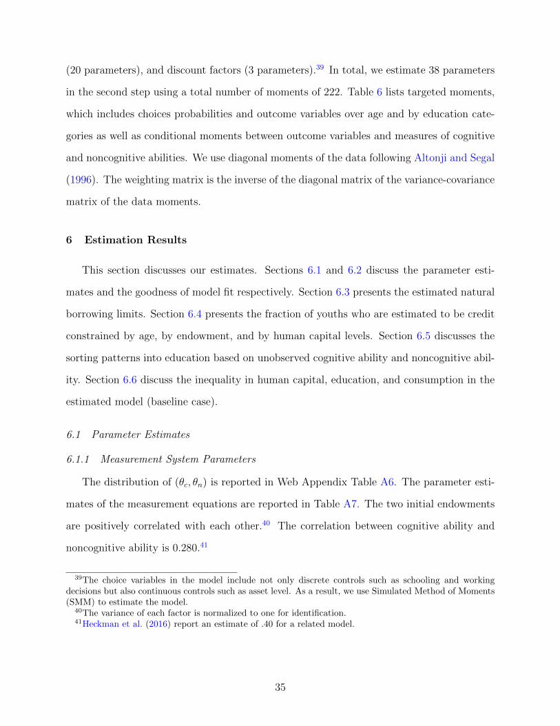
(20 parameters), and discount factors (3 parameters).39 In total, we estimate 38 parameters

in the second step using a total number of moments of 222. Table 6 lists targeted moments,

which includes choices probabilities and outcome variables over age and by education cate-

gories as well as conditional moments between outcome variables and measures of cognitive

and noncognitive abilities. We use diagonal moments of the data following Altonji and Segal

(1996). The weighting matrix is the inverse of the diagonal matrix of the variance-covariance

matrix of the data moments.

6 Estimation Results

This section discusses our estimates. Sections 6.1 and 6.2 discuss the parameter esti-

mates and the goodness of model fit respectively. Section 6.3 presents the estimated natural

borrowing limits. Section 6.4 presents the fraction of youths who are estimated to be credit

constrained by age, by endowment, and by human capital levels. Section 6.5 discusses the

sorting patterns into education based on unobserved cognitive ability and noncognitive abil-

ity. Section 6.6 discuss the inequality in human capital, education, and consumption in the

estimated model (baseline case).

6.1 Parameter Estimates

6.1.1 Measurement System Parameters

The distribution of (θc, θn) is reported in Web Appendix Table A6. The parameter esti-

mates of the measurement equations are reported in Table A7. The two initial endowments

are positively correlated with each other.40 The correlation between cognitive ability and

noncognitive ability is 0.280.41

39The choice variables in the model include not only discrete controls such as schooling and workingdecisions but also continuous controls such as asset level. As a result, we use Simulated Method of Moments(SMM) to estimate the model.

40The variance of each factor is normalized to one for identification.41Heckman et al. (2016) report an estimate of .40 for a related model.

35

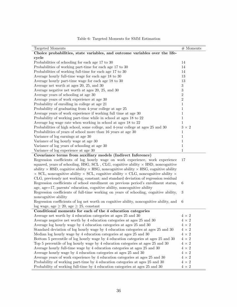
Table 6: Targeted Moments for SMM Estimation

Targeted Moments # MomentsChoice probabilities, state variables, and outcome variables over the life-cycleProbabilities of schooling for each age 17 to 30 14Probabilities of working part-time for each age 17 to 30 14Probabilities of working full-time for each age 17 to 30 14Average hourly full-time wage for each age 18 to 30 13Average hourly part-time wage for each age 18 to 30 13Average net worth at ages 20, 25, and 30 3Average negative net worth at ages 20, 25, and 30 3Average years of schooling at age 30 2Average years of work experience at age 30 2Probability of enrolling in college at age 21 1Probability of graduating from 4-year college at age 25 1Average years of work experience if working full time at age 30 1Probability of working part-time while in school at ages 18 to 22 1Average log wage rate when working in school at ages 18 to 22 1Probabilities of high school, some college, and 4-year college at ages 25 and 30 3 × 2Probabilities of years of school more than 16 years at age 30 1Variance of log earnings at age 30 1Variance of log hourly wage at age 30 1Variance of log years of schooling at age 30 1Variance of log experience at age 30 1Covariance terms from auxiliary models (Indirect Inference)Regression coefficients of log hourly wage on work experience, work experiencesquared, years of schooling, HSG, SCL , CLG, cognitive ability × HSD, noncognitiveability × HSD, cognitive ability × HSG, noncognitive ability × HSG, cognitive ability× SCL, noncognitive ability × SCL, cognitive ability × CLG, noncognitive ability ×CLG, previously not working, constant; and standard deviation of regression residual

17

Regression coefficients of school enrollment on previous period’s enrollment status,age, age=17, parents’ education, cognitive ability, noncognitive ability

6

Regression coefficients of full-time working on years of schooling, cognitive ability,noncognitive ability

3

Regression coefficients of log net worth on cognitive ability, noncognitive ability, andlog wage, age ≥ 20, age ≥ 25, constant

6

Conditional moments for each of the 4 education categoriesAverage net worth by 4 education categories at ages 25 and 30 4 × 2Average negative net worth by 4 education categories at ages 25 and 30 4 × 2Average log hourly wage by 4 education categories at ages 25 and 30 4 × 2Standard deviation of log hourly wage by 4 education categories at ages 25 and 30 4 × 2Median log hourly wage by 4 education categories at ages 25 and 30 4 × 2Bottom 5 percentile of log hourly wage by 4 education categories at ages 25 and 30 4 × 2Top 5 percentile of log hourly wage by 4 education categories at ages 25 and 30 4 × 2Average hourly full-time wage by 4 education categories at ages 25 and 30 4 × 2Average hourly wage by 4 education categories at ages 25 and 30 4 × 2Average years of work experience by 4 education categories at ages 25 and 30 4 × 2Probability of working part-time by 4 education categories at ages 25 and 30 4 × 2Probability of working full-time by 4 education categories at ages 25 and 30 4 × 2

36

6.1.2 Structural Model Parameters

Web Appendix Table A8 reports preference parameter estimates for the schooling utility

functions (Panel A) and work utility function (Panel B). The psychic benefit of schooling

is higher for individuals with higher cognitive and noncognitive abilities. Individuals whose

parents have higher levels of education also have higher flow utility from schooling. The

parameter estimates suggest that the psychic cost of working part-time while in school (φk,e =

−0.0773) is higher than the psychic cost of part-time working while not in school (φk,0 =

−0.0332). In our estimation, we do not impose any restrictions on the relative magnitudes

of these two parameters. Forcing the psychic cost of working part-time while in school to

be the same as the psychic cost of part-time working while not in school overpredicts the

fraction of working students in school.

Parameter estimates of the discount rate function are reported in Table A9. Figure 3

plots the density of estimated discount factors in the benchmark model. Appendix Figure

A4 plots the density of estimated discount factor for high ability and low ability, separately.

As expected, individuals with higher levels of cognitive ability and/or noncognitive ability

have considerably lower rates of time preference.

020

4060

kden

sity

del

ta

.95 .96 .97 .98 .99 Discount Factor

Figure 3: Density of Estimated Discount Factors: exp(−ρ(θc, θn))

37

6.1.3 Labor Market Skill Production and Wages

Table A10 in the Web Appendix reports parameter estimates for the human capital pro-

duction function and the wage equation. A one standard deviation increase in cognitive

ability increases an individual’s human capital level as well as offered wages by

(αψ,c,2 = 0.1433) log points among 4-year college graduate workers. The effects of noncogni-

tive ability on human capital levels and wages are small and not statistically different from

zero.

6.2 Model Goodness of Fit

In this section, we report the goodness of model fit on selected target moments (Table

6 gives the complete set of targeted moments). Our model closely fits the lifecycle patterns

of school enrollment (Figure 4(a)) and employment (see Figures 4(b) and 4(c)). Figure

4(d) shows that our estimated model fits the observed accepted wage patterns over time.

Figures 4(e) and 4(f) plot our model fits of average net worth and average negative net worth

(st1(st < 0)) at ages 20, 25, and 30.42

As shown in Figure 5, our model can replicate the patterns of number of years worked

for each of the four education categories at age 30. Our model can also replicate the average

wages for each education category at age 30.

42Figures A5 in the Web Appendix plots the model fit on years of schooling over age, over parent’seducation categories, and over parents’ net worth terciles. The fit is generally good.

38

0.2

.4.6

.81

In S

choo

l

17 18 19 20 21 22 23 24 25 26 27 Age

95% CI NLSY Data Fitted Model

(a) In School

0.2

.4.6

.81

Wor

k Fu

ll Tim

e

17 18 19 20 21 22 23 24 25 26 27 28 29 30 Age

95% CI NLSY Data Fitted Model

(b) Working Full-time

0.2

.4.6

.81

Wor

k Pa

rt Ti

me

17 18 19 20 21 22 23 24 25 26 27 28 29 30 Age

95% CI NLSY Data Fitted Model

(c) Working Part-time

04

812

1620

2428

Wag

e R

ate

18 19 20 21 22 23 24 25 26 27 28 29 30 Age

95% CI NLSY Data Fitted Model

(d) Hourly Wages over Age

010

000

2000

030

000

4000

050

000

6000

0 N

et W

orth

20 21 22 23 24 25 26 27 28 29 30 Age

95% CI NLSY Data Fitted Model

(e) Net Worth by Age

-800

0-6

000

-400

0-2

000

0

20 21 22 23 24 25 26 27 28 29 30 Age

95% CI NLSY Data Fitted Model

(f) Negative Net Worth by Age

Figure 4: Model Fit over the Lifecycle

02

46

Yrs

of E

xper

ienc

e

< 12 yrs 12 yrs 13 to 15 yrs >=16 yrs Schooling Categories (Age 25)

95% CI NLSY Data Fitted Model

(a) Yrs Worked by Education

04

812

1620

2428

Wag

e R

ate

< 12 yrs 12 yrs 13 to 15 yrs >=16 yrs Schooling Categories (Age 30)

95% CI NLSY Data Fitted Model

(b) Hourly Wages by Education

Figure 5: Model Fit by Education

Tables A11 and A12 in the Web Appendix report model fits for the covariance terms

from auxiliary models for enrollment and employment, respectively. Table A13 in the Web

Appendix reports model fits of the auxiliary model for log hourly wage. Table A14 in the

Web Appendix shows the model fits of the auxiliary model for log net worth. Our model

generally fits the data well.

39

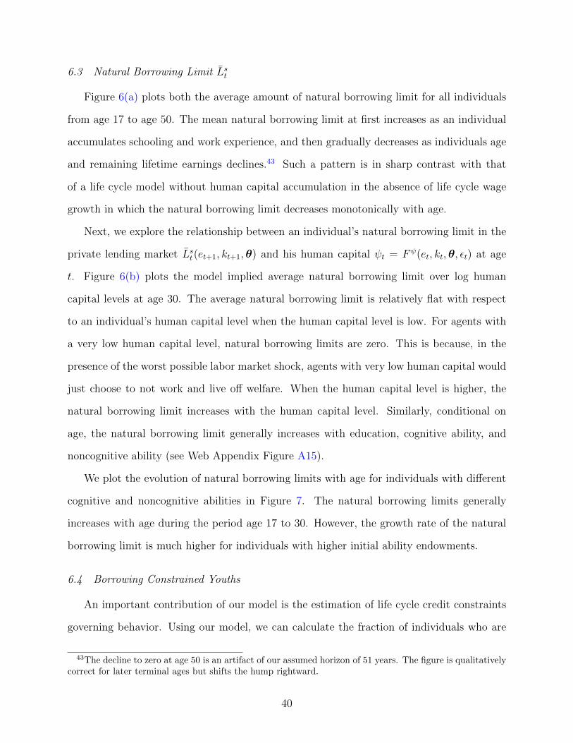
6.3 Natural Borrowing Limit Lst

Figure 6(a) plots both the average amount of natural borrowing limit for all individuals

from age 17 to age 50. The mean natural borrowing limit at first increases as an individual

accumulates schooling and work experience, and then gradually decreases as individuals age

and remaining lifetime earnings declines.43 Such a pattern is in sharp contrast with that

of a life cycle model without human capital accumulation in the absence of life cycle wage

growth in which the natural borrowing limit decreases monotonically with age.

Next, we explore the relationship between an individual’s natural borrowing limit in the

private lending market Lst(et+1, kt+1,θ) and his human capital ψt = Fψ(et, kt,θ, εt) at age

t. Figure 6(b) plots the model implied average natural borrowing limit over log human

capital levels at age 30. The average natural borrowing limit is relatively flat with respect

to an individual’s human capital level when the human capital level is low. For agents with

a very low human capital level, natural borrowing limits are zero. This is because, in the

presence of the worst possible labor market shock, agents with very low human capital would

just choose to not work and live off welfare. When the human capital level is higher, the

natural borrowing limit increases with the human capital level. Similarly, conditional on

age, the natural borrowing limit generally increases with education, cognitive ability, and

noncognitive ability (see Web Appendix Figure A15).

We plot the evolution of natural borrowing limits with age for individuals with different

cognitive and noncognitive abilities in Figure 7. The natural borrowing limits generally

increases with age during the period age 17 to 30. However, the growth rate of the natural

borrowing limit is much higher for individuals with higher initial ability endowments.

6.4 Borrowing Constrained Youths

An important contribution of our model is the estimation of life cycle credit constraints

governing behavior. Using our model, we can calculate the fraction of individuals who are

43The decline to zero at age 50 is an artifact of our assumed horizon of 51 years. The figure is qualitativelycorrect for later terminal ages but shifts the hump rightward.

40

020

0040

0060

0080

00M

ean

Nat

ural

Bor

row

ing

Lim

it

20 25 30 35 40 45 50Age

(a) Natural Borrowing Limit over Ages 17 to 50

050

0010

000

1500

020

000

Nat

ural

Bor

row

ing

Lim

it

1 2 3 4 Log Human Capital (Age 30)

95% CI lpoly smoothkernel = epanechnikov, degree = 0, bandwidth = .23, pwidth = .34

Local polynomial smooth

(b) Natural Borrowing Limit vs Human Capital atAge 30

Figure 6: Mean of Natural Borrowing Limit Lst (et+1, kt+1,θ)

050

0010

000

1500

020

000

Nat

ural

Bor

row

ing

Lim

it

17 18 19 20 21 22 23 24 25 26 27 28 29 30 Cognitive Ability Quartiles

Quartile 1 Quartile 2 Quartile 3 Quartile 4

(a) Natural Borrowing Limit vs Cognitive Ability

050

0010

000

1500

020

000

Nat

ural

Bor

row

ing

Lim

it

17 18 19 20 21 22 23 24 25 26 27 28 29 30 Noncognitive Ability Quartiles

Quartile 1 Quartile 2 Quartile 3 Quartile 4

(b) Natural Borrowing Limit vs Noncog. Ability

Figure 7: Evolution of Average Natural Borrowing Limit by Ability Endowments

41

borrowing-constrained by evaluating the Kuhn-Tucker multiplier associated with an indi-

vidual’s optimal savings decision. In particular, using the first order conditions from an

individual’s optimization problem (Equations (22) and (23)), we can calculate the Kuhn-

Tucker multiplier associated with individuals’ next period asset decisions as follows:

λs,t(ct, st+1; Ωt) =∂uc(ct; Ωt)

∂ct− exp(−ρ(θc, θn))

(∂EVt+1

∂st+1

). (34)

We define an individual as borrowing constrained at period t if λs,t > 0 and st+1 ≤

−Lst(et+1, kt+1,θ). Figures 8, 9, and 10 graph—at ages 21, 30, and 40, respectively—the

model predicted fraction constrained as functions of various arguments. Appendix Fig-

ures A7, A8, and A9 graph the multipliers (λs,t) in the model simulated data as a function

of the same arguments. Figures 8(b), 9(b), and 10(b) report fraction constrained by levels of

cognitive ability. Figures 8(d), 9(d), and 10(d) report fraction constrained by the logarithm

of human capital stocks.

At age 21, these graphs exhibit a weak bimodality that sharpens somewhat by age 30.

Two groups of people are constrained. Many agents with low ability and low human capital

endowments have relatively flat life cycle wage growth. There are also some with high

ability and high human capital endowments with high wage growth who, in their 20s and

early 30s, cannot fully access their future income because of borrowing restrictions. By age

40 (Figure 10), when life cycle earnings growth is more fully realized, the second (already

smaller) hump disappears. The first hump remains throughout the life cycle. The first group

of individuals has low labor market earnings, low savings, and a tight borrowing limits. They

also have high discount rates. These individuals want consumption upfront (even with flat

income profiles) but cannot access it due to their low borrowing limit.44

44Consider a special case where there is no income growth (y1 = y2) and there is no borrowing constraint.The Euler equation for optimal consumption choices indicates that the optimal consumption in periods 1and 2, c∗1 and c∗2, respectively, obey: γ(log c∗2 − log c∗1) = −ρ(θc, θn) + log(1 + r). Therefore, the followingmust be true when there is no borrowing constraint: −ρ(θc, θn) + log(1 + r) < 0 ⇒ c∗2 < c∗1. Thus, whenthe discount rate is relatively high (i.e., the agent is less patient), the agent will try to consume more todayand consume less tomorrow even if there is no income growth between these two periods (y1 = y2). As a

42

There is evidence of bimodality in constraints with respect to cognitive and non-cognitive

ability in the late 20s and early 30s. The patterns with respect to net worth show a sharp

cliff. Beyond a certain level, agents are not constrained.

0.1

.2.3

.4.5

.6.7

.8.9

1Bo

rrow

ing

Con

stra

ined

-50000 0 50000 100000 150000 Net Worth (Age 21)

95% CI lpoly smoothkernel = epanechnikov, degree = 0, bandwidth = 826.85, pwidth = 1240.28

Local polynomial smooth

(a) Fraction Constrained vs st0

.1.2

.3.4

.5.6

.7.8

.91

Borro

win

g C

onst

rain

ed

-4 -2 0 2 4 Cognitive Ability (Age 21)

95% CI lpoly smoothkernel = epanechnikov, degree = 0, bandwidth = .43, pwidth = .64

Local polynomial smooth

(b) Fraction Constrained vs θc

0.1

.2.3

.4.5

.6.7

.8.9

1Bo

rrow

ing

Con

stra

ined

-3 -2 -1 0 1 2 Noncognitive Ability (Age 21)

95% CI lpoly smoothkernel = epanechnikov, degree = 0, bandwidth = .35, pwidth = .53

Local polynomial smooth

(c) Fraction Constrained vs θn

0.1

.2.3

.4.5

.6.7

.8.9

1Bo

rrow

ing

Con

stra

ined

0 1 2 3 4 Log Human Capital (Age 21)

95% CI lpoly smoothkernel = epanechnikov, degree = 0, bandwidth = .12, pwidth = .18

Local polynomial smooth

(d) Fraction Constrained vs logFψ(et, kt,θ, εw,t)

Figure 8: Borrowing Constrained Youths (st+1 ≤ −Lst (et+1, kt+1,θ) & λs,t > 0) at Age 21

Figure 11 shows the life cycle pattern of the proportion borrowing constrained. The

U shape is a consequence of initial borrowing constraints and the approach of the terminal

horizon.45 The constrained in college are 20% more likely to work than other college students.

result, the agent will borrow today to consume more today, and pay back the debt in the next period usingy2 and consume less the next period.

These forces are at work when the agent cannot borrow or cannot borrow enough to reach the optimalconsumption level (c∗1, c

∗2). Low ability individuals with low income growth are borrowing constrained because

they are impatient and their borrowing limit is low.45The age 50 horizon artificially accelerates the borrowing constraint into middle age.

43

0.1

.2.3

.4.5

.6.7

.8.9

1Bo

rrow

ing

Con

stra

ined

-100000 0 100000 200000 300000 400000 Net Worth (Age 30)

95% CI lpoly smoothkernel = epanechnikov, degree = 0, bandwidth = 1157.96, pwidth = 1736.94

Local polynomial smooth

(a) Fraction Constrained vs st

0.1

.2.3

.4.5

.6.7

.8.9

1Bo

rrow

ing

Con

stra

ined

-4 -2 0 2 4 Cognitive Ability (Age 30)

95% CI lpoly smoothkernel = epanechnikov, degree = 0, bandwidth = .24, pwidth = .36

Local polynomial smooth

(b) Fraction Constrained vs θc

0.1

.2.3

.4.5

.6.7

.8.9

1Bo

rrow

ing

Con

stra

ined

-3 -2 -1 0 1 2 Noncognitive Ability (Age 30)

95% CI lpoly smoothkernel = epanechnikov, degree = 0, bandwidth = .23, pwidth = .34

Local polynomial smooth

(c) Fraction Constrained vs θn

0.1

.2.3

.4.5

.6.7

.8.9

1Bo

rrow

ing

Con

stra

ined

1 2 3 4 Log Human Capital (Age 30)

95% CI lpoly smoothkernel = epanechnikov, degree = 0, bandwidth = .17, pwidth = .26

Local polynomial smooth

(d) Fraction Constrained vs logFψ(et, kt,θ, εw,t)

Figure 9: Borrowing Constrained Youths (st+1 ≤ −Lst (et+1, kt+1,θ) & λs,t > 0) at Age 30

44

0.1

.2.3

.4.5

.6.7

.8.9

1Bo

rrow

ing

Con

stra

ined

-100000 0 100000 200000 300000 400000 Net Worth (Age 40)

95% CI lpoly smoothkernel = epanechnikov, degree = 0, bandwidth = 1418.7, pwidth = 2128.05

Local polynomial smooth

(a) Fraction Constrained vs st

0.1

.2.3

.4.5

.6.7

.8.9

1Bo

rrow

ing

Con

stra

ined

-4 -2 0 2 4 Cognitive Ability (Age 40)

95% CI lpoly smoothkernel = epanechnikov, degree = 0, bandwidth = .61, pwidth = .92

Local polynomial smooth

(b) Fraction Constrained vs θc

0.1

.2.3

.4.5

.6.7

.8.9

1Bo

rrow

ing

Con

stra

ined

-3 -2 -1 0 1 2 Noncognitive Ability (Age 40)

95% CI lpoly smoothkernel = epanechnikov, degree = 0, bandwidth = .59, pwidth = .88

Local polynomial smooth

(c) Fraction Constrained vs θn

0.1

.2.3

.4.5

.6.7

.8.9

1Bo

rrow

ing

Con

stra

ined

1 2 3 4 5 Log Human Capital (Age 40)

95% CI lpoly smoothkernel = epanechnikov, degree = 0, bandwidth = .19, pwidth = .28

Local polynomial smooth

(d) Fraction Constrained vs logFψ(et, kt,θ, εw,t)

Figure 10: Borrowing Constrained Youths (st+1 ≤ −Lst (et+1, kt+1,θ) & λs,t > 0) at Age 40

0.1

.2.3

.4Fr

actio

n Bo

rrow

ing

Con

stra

ined

20 25 30 35 40 45 50Age

Figure 11: % Borrowing Constrained by Age

45

6.5 Sorting into Education by Ability

Simulating our model, we illustrate the magnitude of sorting into education at age 30

based on unobserved abilities. Figure 12 is the density plot of the two unobservabled factors

by education groups in the simulated data.

As seen in Figure 12, people sort into education based on cognitive and noncognitive

ability. On average, individuals who obtain higher education are more likely to have greater

cognitive ability and noncognitive ability. However, there is also substantial overlap in both

cognitive ability and noncognitive ability levels across different schooling levels, suggesting

that sorting based on abilities is not the only factor shaping individual educational outcomes.

0.1

.2.3

.4.5

Density

−4 −2 0 2 4 Cognitive Ability

< 12 yrs 12 yrs

13 to 15 yrs >=16 yrs

0.2

.4.6

Density

−3 −2 −1 0 1 2 Noncognitive Ability

< 12 yrs 12 yrs

13 to 15 yrs >=16 yrs

Figure 12: Density of Initial Factors Conditional on Age-30 Education

6.6 Inequality in Education, Wages, and Consumption

Both employment decisions and borrowing constraints have important consequences for

wage and consumption inequality.46 The first row of Table 7 shows the age-30 inequality in

education, wages, and consumption in our benchmark model. Cross-sectional inequality is

measured by the variance of logs. Wage inequality is higher than education inequality because

of the existence of uninsured human capital risk, and large variation in individuals’ work

experience, cognitive ability, and noncognitive ability. Consumption inequality is lower than

46The model simulated consumption should be interpreted as all consumption expenditure including rentalequivalent consumption values for homeowners and rents for non-homeowners.

46

wage earning inequality because individuals use savings to smooth consumption fluctuations.

We discuss the other rows of this table in the next section when we discuss counterfactuals.

Table 7: Inequality in Education, Wages, and Consumption (Age 30)

Inequality (Var of log) Changes in Inequality (%)

Educ Wage C Educ Wage C

Benchmark 0.0395 0.3313 0.1002 N.A. N.A. N.A.

Counterfactual Experiments

Equalizing Cognitive Ability 0.0255 0.2924 0.0714 -35.53 -11.75 -28.73

Equalizing Noncognitive Ability 0.0222 0.3012 0.0775 -43.88 -9.08 -22.69

Equalizing Parental Factors 0.0363 0.3292 0.0963 -8.14 -0.64 -3.92

Note: Inequality in education (Educ), wage, and consumption (C) are measured using variance of log yearsof schooling, log hourly wage rates, and log consumption at age 30, respectively. Changes in inequality iscalculated as the percentage changes in inequality compared to the benchmark model. When equalizingcognitive ability, we set every individual’s cognitive ability equal to the population mean, i.e., zero.Similarly, we set every individual’s noncognitive ability equal to zero when equalizing noncognitive ability.When equalizing parental factors, we set parents’ education equal to 12 years of schooling and parent’s networth to be in the second tercile. Once cognitive ability, noncognitive ability, and parental factors are allequalized, the variance remains are: Var(log (Educ)) = 0.0055, Var(log (Wage)) = 0.2623, and Var(log (C))= 0.0432.

7 Counterfactual Exercises

In this section of the paper, we use our model to examine the impacts of changing credit

constraints, tuition, and initial endowments on inequality. We start by analyzing the impact

of equalizing endowments.

7.1 Equalizing Initial Endowments

We address the following question: To what extent do differences in cognitive ability,

noncognitive ability, and parental environments account for the observed cross-section in-

equality in years of schooling, earnings, and consumption at age 30? To address this question,

we perform three counterfactual experiments that equalize initial heterogeneity in (i) cogni-

tive ability, (ii) noncognitive ability, and (iii) parental background factors (including both

47

schooling and net worth). Equalization is achieved by placing all observations at the means

of the selected variable, keeping other variables at sample values.

As shown in Table 7, equalizing cognitive ability reduces age-30 inequality in education by

36%. Equalizing noncognitive ability reduces age-30 education inequality by 44%. Finally,

equalizing parental factors (including parent’s education and net worth) reduces inequality

by 8%. Equalizing cognitive endowments reduces wage inequality by 12% and consumption

inequality by 29%. Equalizing noncognitive endowments reduces wage inequality by 9%

and consumption inequality by 23%. Equalizing parental factors has little impact on wage

inequality, and it reduces consumption inequality by 4%.

We also investigate the effects of cognitive ability, noncognitive ability and parental fac-

tors on the youths’ age-17 present discounted lifetime utility inequality. Equalizing cognitive

ability reduces age-17 present discounted lifetime utility inequality by 24%. Equalizing

noncognitive ability reduces age-17 present discounted lifetime utility inequality by 91%.

Equalizing parental factors (including parent’s education and net worth) reduces age-17

present discounted lifetime utility inequality by 2%. The age-17 present discounted life-

time utility inequality equal to zero once cognitive ability, noncognitive ability, and parental

factors are all equalized.

Table 8: Years of Schooling and College Attendance and Graduation under Different Experiments

Years ofSchooling at

Age 30

CollegeAttendance at

Age 21 (%)

4-Year CollegeGraduation at

Age 25 (%)

% Studentswho WorkPart-Time

Benchmark 13.76 47.25 27.76 63.45

Counterfactual Experiments Changes Relative to Benchmark(1) Subsidizing College Tuition 0.18 6.22 3.55 -5.72(2) Increasing Student Loan Limits 0.04 3.95 1.09 1.28

Note: Education is measured by the average years of schooling at age 30. College attendance is measuredas the percentage of individuals whose years of education is more than or equal to 13 at age 21. The rate of4-year college graduation is measured as the percentage of individuals whose years of schooling is morethan or equal to 16 at age 25. The fraction of students who work part-time while in school are calculatedover age 18 to 22.

48

7.2 Subsidizing College Tuition

We next consider the impact of subsidizing tuition on schooling choices. We give each

agent a college tuition subsidy of $1,500 per year, which amounts to 29% of average college

tuition cost and fees minus grants and scholarship.47 As shown in Table 8, compared to

the benchmark model, the college attendance rate at age 21 increases by 6.22 percentage

points (13.17%). The implied elasticity of college going with respect to tuition is −0.45,

which is within the range of estimates reported in the literature.48 This tuition subsidy

policy also leads to 3.55 percentage point increase in the 4-year college graduation rate at

age 25. The college tuition subsidy reduces students’ incentive to work while in school. In

particular, under this policy, the fraction of students who work part-time at school decreases

by 6 percentage points.

Figure 13 plots the college attendance and the 4-year college graduation rates for the

benchmark and tuition subsidy policy over the full distribution of cognitive ability and

noncognitive ability. Our college tuition subsidy increases college attendance at age 21 among

the individuals whose cognitive ability is within the second and third quartiles. The rate of

4-year college graduation increases much more among high ability individuals compared to

that among low ability individuals.

7.3 Increasing Student Loan Limits

We next consider the impact of increasing student loan limits. In this counterfactual

experiment, we increase the borrowing limit from the student program by $1,500 for each

academic year, which amounts to a 29% reduction of average college tuition costs and fees

minus grants and scholarship. As shown in Table 8, compared to the benchmark model, the

college attendance rate at age 21 increases by 4.0 percentage points and the 4-year college

graduation rate at age 25 barely increases. Under the student loan enhancement policy,

47In the simulation, we do not allow the amount of student loan that an individual can borrow if he decidesto attend college to be directly affected by such college tuition subsidy.

48See, e.g., Cameron and Heckman (2001) and Heckman and Cameron (1999).

49

0.1

.2.3

.4.5

.6.7

.8.9

1 C

olle

ge A

ttend

ance

Quartile 1 Quartile 2 Quartile 3 Quartile 4 Cognitive Ability Quartiles

Fitted Model CF: Subsidizing College Tuition

(a) College Attendance & Cognitive Ability (Age21)

0.1

.2.3

.4.5

.6.7

.8.9

1 C

olle

ge A

ttend

ance

Quartile 1 Quartile 2 Quartile 3 Quartile 4 Noncognitive Ability Quartiles

Fitted Model CF: Subsidizing College Tuition

(b) College Attendance & Noncognitive Ability(Age 21)

0.1

.2.3

.4.5

.6.7

.8.9

1 4

-Yr C

olle

ge G

radu

atio

n

Quartile 1 Quartile 2 Quartile 3 Quartile 4 Cognitive Ability Quartiles

Fitted Model CF: Subsidizing College Tuition

(c) 4-Year College & Cognitive Ability (Age 25)

0.1

.2.3

.4.5

.6.7

.8.9

1 4

-Yr C

olle

ge G

radu

atio

n

Quartile 1 Quartile 2 Quartile 3 Quartile 4 Noncognitive Ability Quartiles

Fitted Model CF: Subsidizing College Tuition

(d) 4-Year College & Noncognitive Ability (Age25)

Figure 13: Effects of College Tuition Subsidy

the fraction of students who work part-time in school increases in response to the increased

student debt limits. However such increases are small (1 percentage point).

Figure 14 plots the college attendance and the 4-year college graduation rates for the

benchmark and enhanced student loan limit policy over the full distribution of cognitive

ability and noncognitive ability. The differences are small.49 There appears to be a limited

role for policies enhancing student access to credit for promoting college attendance and

graduation.

49These results are comparable to those reported in Johnson (2013).

50

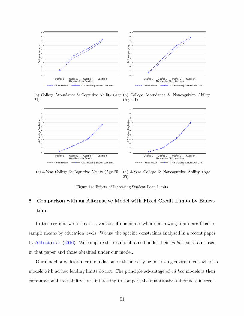
0.1

.2.3

.4.5

.6.7

.8.9

1 C

olle

ge A

ttend

ance

Quartile 1 Quartile 2 Quartile 3 Quartile 4 Cognitive Ability Quartiles

Fitted Model CF: Increasing Student Loan Limit

(a) College Attendance & Cognitive Ability (Age21)

0.1

.2.3

.4.5

.6.7

.8.9

1 C

olle

ge A

ttend

ance

Quartile 1 Quartile 2 Quartile 3 Quartile 4 Noncognitive Ability Quartiles

Fitted Model CF: Increasing Student Loan Limit

(b) College Attendance & Noncognitive Ability(Age 21)

0.1

.2.3

.4.5

.6.7

.8.9

1 4

-Yr C

olle

ge G

radu

atio

n

Quartile 1 Quartile 2 Quartile 3 Quartile 4 Cognitive Ability Quartiles

Fitted Model CF: Increasing Student Loan Limit

(c) 4-Year College & Cognitive Ability (Age 25)

0.1

.2.3

.4.5

.6.7

.8.9

1 4

-Yr C

olle

ge G

radu

atio

n

Quartile 1 Quartile 2 Quartile 3 Quartile 4 Noncognitive Ability Quartiles

Fitted Model CF: Increasing Student Loan Limit

(d) 4-Year College & Noncognitive Ability (Age25)

Figure 14: Effects of Increasing Student Loan Limits

8 Comparison with an Alternative Model with Fixed Credit Limits by Educa-

tion

In this section, we estimate a version of our model where borrowing limits are fixed to

sample means by education levels. We use the specific constraints analyzed in a recent paper

by Abbott et al. (2016). We compare the results obtained under their ad hoc constraint used

in that paper and those obtained under our model.

Our model provides a micro-foundation for the underlying borrowing environment, whereas

models with ad hoc lending limits do not. The principle advantage of ad hoc models is their

computational tractability. It is interesting to compare the quantitative differences in terms

51

of parameter estimates, model fits, model predictions, and counterfactual implications.

We follow Abbott et al. (2016) and consider the following specification of credit limits:50

Lst(e) =

$75, 000 if e ≥ 16

$25, 000 if e < 16 & e ≥ 12

$15, 000 if e < 12

(35)

if t ≥ 22 and Lst(e) = 0 if t < 22. They justify these limits using averages of self-reported

credit limits in the survey of consumer finances.

We apply the same estimation procedure (see Section 5) to estimate this alternative

model and estimate the same set of structural parameters. Our model with endogenous debt

limit is a far more stringent approach to estimation than models with ad hoc credit limits.

8.1 Estimation Results

The last two columns of Web Appendix Table A8 report preference parameter estimates

for the schooling utility functions (Panel A) and work utility function (Panel B) in the

alternative model. Similar to our model with endogenous credit constraints, we find that he

psychic benefit of schooling is higher for individuals with higher cognitive and noncognitive

abilities, and is higher if their parents have higher education. We also find that the psychic

cost of working part-time while in school (φk,e = −0.0603) is higher than the psychic cost

of part-time working while not in school (φk,0 = −0.0338). These estimates are similar in

magnitude to those estimated for our model with endogenous credit constraints.

One of the biggest differences in the estimated parameter values between our model and

the alternative model lies in the estimated parameter values for the subjective discount rate.

In particular, in the alternative model, the estimated discount factor is much higher, which

50In Abbott et al. (2016), among working-age married households, borrowing limit equals to $75,000 if themost educated spouse is a college graduate, $25,000 if the most educated spouse is a high school graduate,and $15,000 if both spouses are high school dropouts; No borrowing before age 21. Borrowing limits basedon self-reported limits on unsecured credit by family type from SCF.

52

implies that individuals are more patient (see Table A9 to compare parameter estimates).

Figure 15 plots the distribution of estimated discount factors. Appendix Figure 4(c) plots

the density of estimated discount factor for high cognitive ability and low cognitive abil-

ity. Appendix Figure 4(d) plots the density of estimated discount factor for high cognitive

noncognitive ability and low noncognitive ability. As in our model, those with higher cogni-

tive and/or noncognitive skills have lower rates of time preference.0

2040

6080

kden

sity

del

ta

.965 .97 .975 .98 .985 .99 Discount Factor

Figure 15: Density of Estimated Discount Factors (Fixed Credit Limits by Education): exp(−ρ(θc, θn))

This has important implications for the estimated levels of human and physical capital

accumulation. The overall fit of this model to the data is worse than our model. The

minimized SMM objective function in this model is 76% larger than in our model with

endogenous credit constraints. The fit of the model to the data is worse for many components

of life cycle behavior than our model (for example, compare Figures 16 and 17 with Figures 4

and 5, and appendix Table A14). Sorting patterns into education by ability are similar (see

Figure 18).

53

0.2

.4.6

.81

In S

choo

l

17 18 19 20 21 22 23 24 25 26 27 Age

95% CI NLSY Data Fitted Model

(a) In School

0.2

.4.6

.81

Wor

k Fu

ll Tim

e

17 18 19 20 21 22 23 24 25 26 27 28 29 30 Age

95% CI NLSY Data Fitted Model

(b) Working Full-time

0.2

.4.6

.81

Wor

k Pa

rt Ti

me

17 18 19 20 21 22 23 24 25 26 27 28 29 30 Age

95% CI NLSY Data Fitted Model

(c) Working Part-time

04

812

1620

2428

Wag

e R

ate

18 19 20 21 22 23 24 25 26 27 28 29 30 Age

95% CI NLSY Data Fitted Model

(d) Hourly Wages over Age

010

000

2000

030

000

4000

050

000

6000

0 N

et W

orth

20 21 22 23 24 25 26 27 28 29 30 Age

95% CI NLSY Data Fitted Model

(e) Net Worth by Age

-800

0-6

000

-400

0-2

000

0

20 21 22 23 24 25 26 27 28 29 30 Age

95% CI NLSY Data Fitted Model

(f) Negative Net Worth by Age

Figure 16: Goodness of Fit over the Lifecycle (Alternative Model)

02

46

Yrs

of E

xper

ienc

e

< 12 yrs 12 yrs 13 to 15 yrs >=16 yrs Schooling Categories (Age 25)

95% CI NLSY Data Fitted Model

(a) Yrs Worked by Education

04

812

1620

2428

Wag

e R

ate

< 12 yrs 12 yrs 13 to 15 yrs >=16 yrs Schooling Categories (Age 30)

95% CI NLSY Data Fitted Model

(b) Hourly Wages by Education

Figure 17: Goodness of Fit by Education (Alternative Model)

Similar to our analysis of the model with endogenous credit constraints, we also report

the evolution of credit limit for the Abbott et al. model. In the ad hoc model, the credit limit

does not change with age or work experience after the agent completes the highest degree

(see Web Appendix Figure A10(a)). Conditional on age, the credit limit is bounded below

at $15,000 and increases with human capital, which is due to the fact on average higher

educated individuals have higher human capital level (Web Appendix Figure A10(b)). At

age 30, the borrowing limit increases with education, cognitive ability, and noncognitive

54

0.1

.2.3

.4.5

Density

−4 −2 0 2 4 Cognitive Ability

< 12 yrs 12 yrs

13 to 15 yrs >=16 yrs

0.2

.4.6

Density

−3 −2 −1 0 1 2 Noncognitive Ability

< 12 yrs 12 yrs

13 to 15 yrs >=16 yrs

Figure 18: Density of Initial Factors Conditional on Age-30 Education (Alternative Model)

ability; but there is no heterogeneity in credit limits within each education category (see

Web Appendix Figure A15).

The estimated patterns of constraints by age and individual characteristics are different

across the two models. The age 21 patterns are roughly similar, but the hump is more

noticeable in the ad hoc model. The weak bimodality at age 30 found in our model is not

present in the ad hoc model, and the proportion of agents constrained is much lower. The

fraction of borrowing constrained population continues to decrease and reaches zero after

age 45 (Figure 19).51

0.1

.2.3

.4Fr

actio

n Bo

rrow

ing

Con

stra

ined

20 25 30 35 40 45 50Age

Figure 19: % Borrowing Constrained by Age for Alternative Model

51After college is completed, the private debt limit in the ad hoc model is set at a very large number.

55

8.2 Counterfactual Experiments

Differences are sharp between the two models when we consider the same set of policy

experiments conducted for our model with endogenous credit constraints. We consider the

implications of changing endowments, tuition and credit limits in the ad hoc model for the

same set of policies considered in the discussion of the endogenous credit constrained model.

We start by equalizing initial endowments.

8.2.1 Equalizing Initial Endowments

As shown in Table 9, equalizing cognitive ability reduces age-30 inequality in education by

36% (about the same as in the model with endogenous constraints). Equalizing noncognitive

ability reduces age-30 education inequality by 38% – less than in our model (44%). Finally,

equalizing parental factors (including parent’s education and net worth) reduces inequality

by 6% (compared to 8% for our model). These equalizing effects are generally smaller than

in the model with endogenous credit constraints.

Equalizing cognitive endowments reduces wage inequality by 12% (about the same as in

the model with endogenous constraints) and consumption inequality by 40% (compared to

29% for our model). Equalizing noncognitive endowments reduces wage inequality by 9%

(vs 9%) and consumption inequality by 33% (vs 23%). Equalizing parental factors has little

impact on wage inequality, and reduces consumption inequality by 5% (compared to 4% for

our model).

56

Table 9: Inequality in Education, Wages, and Consumption at Age 30 (Fixed Credit Limits by Education)

Inequality (Var of log) Changes in Inequality (%)

Educ Wages C Educ Wages C

Benchmark 0.0398 0.3825 0.1168 N.A. N.A. N.A.

Counterfactual Experiments

Equalizing Cognitive Ability 0.0253 0.3360 0.0704 -36.37 -12.17 -39.75

Equalizing Noncognitive Ability 0.0248 0.3471 0.0784 -37.76 -9.27 -32.89

Equalizing Parental Factors 0.0375 0.3782 0.1112 -5.75 -1.14 -4.83

Note: Inequality in Education (Educ), wages, and consumption (C) are measured using variance of logyears of schooling, log hourly wage rates, and log consumption at age 30, respectively. Changes ininequality is calculated as the percentage changes in inequality compared to the benchmark model. Whenequalizing cognitive ability, we set every individual’s cognitive ability equal to the population mean, i.e.,zero. Similarly, we set every individual’s noncognitive ability equal to zero when equalizing noncognitiveability. When equalizing parental factors, we set parents’ education equal to 12 years of schooling andparent’s net worth to be in the second tercile.

Table 10: Years of Schooling and College Attendance and Graduation under Different Experiments (FixedCredit Limits by Education)

Years ofSchooling at

Age 30

CollegeAttendance at

Age 21 (%)

4-Year CollegeGraduation at

Age 25 (%)

% Studentswho WorkPart-Time

Benchmark 13.52 48.44 34.53 64.83

Counterfactual Experiments Changes Relative to Benchmark(1) Subsidizing College Tuition 0.29 7.63 5.78 -5.11(2) Increasing Student Loan Limits 0.12 4.60 2.34 0.60

Note: Education is measured by the average years of schooling at age 30. College attendance is measuredas the percentage of individuals whose years of education is more than or equal to 13 at age 21. The rate of4-year college graduation is measured as the percentage of individuals whose years of schooling is morethan or equal to 16 at age 25. The fraction of students who work part-time while in school are calculatedover age 18 to 22.

8.2.2 Subsidizing College Tuition

This section reports the effects of a tuition subsidy on schooling choices. We give each

agent a college tuition subsidy of $1,500 per year, which amounts to 29% of average college

57

tuition cost and fees minus grants and scholarship.52 As shown in Table 10, compared to the

benchmark model, the college attendance rate at age 21 increases by 7.63 percentage points

(15.76%). The implied elasticity of college going with respect to tuition is −0.54, which is

much higher than the elasticity obtained in the model with endogenous credit limits. Such

a tuition subsidy policy also leads to 5.78 percentage points increase in the 4-year college

graduation rate at age 25. The fraction of students age 18 to 22 who work part-time at

school decreases by 5.1 percentage points.

0.1

.2.3

.4.5

.6.7

.8.9

1 C

olle

ge A

ttend

ance

Quartile 1 Quartile 2 Quartile 3 Quartile 4 Cognitive Ability Quartiles

Fitted Model CF: Subsidizing College Tuition

(a) College Attendance & Cognitive Ability (Age21)

0.1

.2.3

.4.5

.6.7

.8.9

1 C

olle

ge A

ttend

ance

Quartile 1 Quartile 2 Quartile 3 Quartile 4 Noncognitive Ability Quartiles

Fitted Model CF: Subsidizing College Tuition

(b) College Attendance & Noncognitive Ability(Age 21)

0.1

.2.3

.4.5

.6.7

.8.9

1 4

-Yr C

olle

ge G

radu

atio

n

Quartile 1 Quartile 2 Quartile 3 Quartile 4 Cognitive Ability Quartiles

Fitted Model CF: Subsidizing College Tuition

(c) 4-Year College & Cognitive Ability (Age 25)

0.1

.2.3

.4.5

.6.7

.8.9

1 4

-Yr C

olle

ge G

radu

atio

n

Quartile 1 Quartile 2 Quartile 3 Quartile 4 Noncognitive Ability Quartiles

Fitted Model CF: Subsidizing College Tuition

(d) 4-Year College & Noncognitive Ability (Age25)

Figure 20: Effects of College Tuition Subsidy on Attendance and Graduation (Fixed Credit Limits byEducation)

52In the simulation, we do not allow the amount of student loan that an individual can borrow if he decidesto attend college to be directly affected by such college tuition subsidy.

58

Figure 20 plots the college attendance and the 4-year college graduation rates for the

benchmark and reduced tuition policy over the full distribution of cognitive ability and

noncognitive ability. The college tuition subsidy increases the college attendance at age 21

for all quartiles of cognitive ability, including those located at the lowest cognitive ability

quartile.

In summary, the model with education-specific fixed credit limits predicts a higher elas-

ticity of response to tuition than the model with an endogenous borrowing limit. Ad hoc

credit limits of the sort used by Abbott et al. (2016) overstate somewhat the effectiveness

of a tuition-reduction policy. This finding is intuitive because restricting borrowing limits

to be the same within each education group over-predicts the amount of debt a low-ability

individual can borrow from private debt market and thus over-predicts the net benefits of

college education for low ability students. In our model, even after conditioning on educa-

tion, our model predicts that the amount of debt an individual can borrow is lower if the

individual has lower human capital (either due to low abilities or low work experience) and

if the individual has a higher psychic cost of working.

8.2.3 Increasing Student Loan Limits

In this counterfactual experiment, we increase the borrowing limit from the student

program by $1,500 for each academic year (the same as in the analysis of our model). As

shown in Table 10, such policy experiments lead to a 4.60 percentage point increase in the

college attendance rate at age 21 and 2.34 percentage points increase in the 4-year college

graduation rate at age 25. The fraction of students age 18 to 22 who work part-time while

in school increases by 0.6 percentage points. Figure 21 plots the college attendance and the

4-year college graduation rates for the benchmark and enhanced student loan limit policy

over the full distribution of cognitive ability and noncognitive ability. The differences are

small.53 These results are comparable to those obtained from the model with endogenous

53These results are comparable to those reported in Johnson (2013).

59

credit constraints.

0.1

.2.3

.4.5

.6.7

.8.9

1 C

olle

ge A

ttend

ance

Quartile 1 Quartile 2 Quartile 3 Quartile 4 Cognitive Ability Quartiles

Fitted Model CF: Increasing Student Loan Limit

(a) College Attendance & Cognitive Ability (Age21)

0.1

.2.3

.4.5

.6.7

.8.9

1 C

olle

ge A

ttend

ance

Quartile 1 Quartile 2 Quartile 3 Quartile 4 Noncognitive Ability Quartiles

Fitted Model CF: Increasing Student Loan Limit

(b) College Attendance & Noncognitive Ability(Age 21)

0.1

.2.3

.4.5

.6.7

.8.9

1 4

-Yr C

olle

ge G

radu

atio

n

Quartile 1 Quartile 2 Quartile 3 Quartile 4 Cognitive Ability Quartiles

Fitted Model CF: Increasing Student Loan Limit

(c) 4-Year College & Cognitive Ability (Age 25)

0.1

.2.3

.4.5

.6.7

.8.9

1 4

-Yr C

olle

ge G

radu

atio

n

Quartile 1 Quartile 2 Quartile 3 Quartile 4 Noncognitive Ability Quartiles

Fitted Model CF: Increasing Student Loan Limit

(d) 4-Year College & Noncognitive Ability (Age25)

Figure 21: Effects of Increasing Student Loan Limits on Attendance and Graduation (Fixed Credit Limitsby Education)

60

9 Summary and Conclusion

This paper estimates a life cycle model of human capital and work experience with

parental transfers in the presence of endogenous borrowing limits and precautionary savings

motives. In our model, individuals are subject to uninsured human capital risks and choose

to invest in education, accumulate work experience and assets, and smooth consumption.

Borrowing is permitted up to an endogenously determined limit. The limit is explicitly

derived. Our model extends Aiyagari’s (1994) analysis by considering the effects of labor

supply and human capital accumulation on the supply of available credit. We account for the

private lending market and government student loan programs. We use our estimated model

to investigate the determinants of human capital inequality and to examine the relationship

between educational attainment, cognitive and noncognitive abilities, and parental education

and wealth. We analyze the effects of tuition subsidies and enhanced student loan limits

on educational attainment and human capital inequality. We do not introduce arbitrary

free parameters into our analysis of credit constraints, nor do we impose ad hoc borrowing

constraints.

We find substantial evidence of life cycle credit constraints that affect human capital

accumulation and inequality. Constrained individuals fall into two groups. A large propor-

tion of the chronically poor with low initial endowments and abilities who acquire little skill

over their lifetimes are constrained. There is also a smaller portion of initially well-endowed

persons with high levels of acquired skills who are constrained early in their life cycles. The

first group has flat life cycle wage profiles. Most remain constrained over their lifetimes. The

second group has rising life cycle wage profiles. They are constrained only early on in life

because they cannot immediately access their future earnings. As they age, their constraints

are relaxed as they access their future earnings.

Equalizing cognitive and noncognitive ability (separately and together) has dramatic

effects on reducing inequality in education. Equalizing parental backgrounds has a much

weaker effect on inequality in earnings and consumption. Reducing tuition has substantial

61

impacts on schooling, but has only minor effects on our measures of inequality (even lifetime

utility). Enhancing student loan limits has minor effects on all outcomes studied.

We compare the estimates from our model with those from a recent model that im-

poses ad hoc credit constraints by education level. There are differences in the predictions

across models. The ad hoc approach overstates the likely effectiveness of tuition policy and

understates the fraction of individuals who are constrained.

Acknowledgements

We thank Dean Corbae, Mariacristina De Nardi, Lance Lochner, Steve Stern, and par-ticipants at the Human Capital and Inequality Conference held at Chicago on December17th, 2015, for helpful comments and suggestions on an earlier draft of this paper. Wealso thank Joseph Altonji, Peter Arcidiacono, Panle Jia Barwick, Jeremy Fox, Jorge Garcıa,Limor Golan, Lars Hansen, John Kennan, Rasmus Lentz, Maurizio Mazzocco, Aloysius Siow,Ronni Pavan, John Rust, Bertel Schjerning, Christopher Taber, and participants at theCowles Conference in Structural Microeconomics and the Stanford Institute for TheoreticalEconomics (SITE) Summer Workshop for helpful comments. We also thank two anony-mous referees. Yu Kyung Koh provided very helpful comments on this paper. This researchwas supported in part by: the Pritzker Children’s Initiative; the Buffett Early ChildhoodFund; NIH grants NICHD R37HD065072, NICHD R01HD054702, and NIA R24AG048081;an anonymous funder; Successful Pathways from School to Work, an initiative of the Univer-sity of Chicago’s Committee on Education and funded by the Hymen Milgrom SupportingOrganization; the Human Capital and Economic Opportunity Global Working Group, aninitiative of the Center for the Economics of Human Development and funded by the Insti-tute for New Economic Thinking; and the American Bar Foundation. The views expressedin this paper are solely those of the authors and do not necessarily represent those of thefunders or the official views of the National Institutes of Health. The Web Appendix for thispaper is located at https://cehd.uchicago.edu/human-capital-constraints.

62

Abbott, B., Gallipoli, G., Meghir, C., Violante, G. L., March 2016. Education policy and

intergenerational transfers in equilibrium, under revision, Journal of Political Economy.

Aiyagari, S. R., August 1994. Uninsured idiosyncratic risk and aggregate saving. Quarterly

Journal of Economics 109 (3), 659–684.

Albuquerque, R., Hopenhayn, H. A., 2004. Optimal lending contracts and firm dynamics.

Review of Economic Studies 71 (2), 285–315.

Altonji, J. G., Segal, L. M., July 1996. Small-sample bias in GMM estimation of covariance

structures. Journal of Business and Economic Statistics 14 (3), 353–366.

Alvarez, F., Jermann, U. J., 2001. Quantitative asset pricing implications of endogenous

solvency constraints. Review of Financial Studies 14 (4), 1117–1151.

Anderson, T. W., Rubin, H., 1956. Statistical inference in factor analysis. In: Neyman,

J. (Ed.), Proceedings of the Third Berkeley Symposium on Mathematical Statistics and

Probability. Vol. 5. University of California Press, Berkeley, CA, pp. 111–150.

Bailey, M. J., Dynarski, S. M., 2011. Inequality in postsecondary education. In: Duncan,

G. J., Murnane, R. J. (Eds.), Whither Opportunity? Rising Inequality, Schools, and

Children’s Life Chances. Russell Sage Foundation, New York, Ch. 6, pp. 117–132.

Belley, P., Lochner, L., December 2007. The changing role of family income and ability in

determining educational achievement. Journal of Human Capital 1 (1), 37–89.

Blundell, R., Costa Dias, M., Meghir, C., Shaw, J., September 2016. Female labor supply,

human capital, and welfare reform. Econometrica 84 (5), 1705–1753.

Browning, M., Hansen, L. P., Heckman, J. J., 1999. Micro data and general equilibrium

models. In: Taylor, J. B., Woodford, M. (Eds.), Handbook of Macroeconomics. Vol. 1A.

Elsevier B. V., Amsterdam, Ch. 8, pp. 543–633.

63

Cagetti, M., De Nardi, M., October 2006. Entrepreneurship, frictions, and wealth. Journal

of Political Economy 114 (5), 835–870.

Cameron, S. V., Heckman, J. J., June 2001. The dynamics of educational attainment for

black, Hispanic, and white males. Journal of Political Economy 109 (3), 455–499.

Cameron, S. V., Taber, C., February 2004. Estimation of educational borrowing constraints

using returns to schooling. Journal of Political Economy 112 (1), 132–182.

Carneiro, P., Heckman, J. J., October 2002. The evidence on credit constraints in post-

secondary schooling. Economic Journal 112 (482), 705–734.

Caucutt, E. M., Lochner, L. J., October 2012. Early and late human capital investments,

borrowing constraints, and the family. Working Paper 18493, National Bureau of Economic

Research.

Chatterjee, S., Corbae, D., Nakajima, M., Rıos-Rull, J.-V., November 2007. A quantitative

theory of unsecured consumer credit with risk of default. Econometrica 75 (6), 1525–1589.

Cooley, T., Marimon, R., Quadrini, V., 2004. Aggregate consequences of limited contract

enforceability. Journal of Political Economy 112 (4), 817–847.

Cunha, F., Heckman, J. J., Fall 2008. Formulating, identifying and estimating the technology

of cognitive and noncognitive skill formation. Journal of Human Resources 43 (4), 738–782.

Cunha, F., Heckman, J. J., Schennach, S. M., May 2010. Estimating the technology of

cognitive and noncognitive skill formation. Econometrica 78 (3), 883–931.

De Nardi, M., 2004. Wealth inequality and intergenerational links. Review of Economic

Studies 71 (3), 743–768.

Fernandez-Villaverde, J., Krueger, D., August 2007. Consumption over the life cycle: Facts

from consumer expenditure survey data. Review of Economics and Statistics 89 (3), 552–

565.

64

Gertler, M., Kiyotaki, N., 2010. Financial intermediation and credit policy in business cycle

analysis. In: Friedman, B. M., Woodford, M. (Eds.), Handbook of Monetary Economics.

Vol. 3. Elsevier B. V., Amsterdam, Ch. 11, pp. 547–599.

Gourinchas, P.-O., Parker, J. A., January 2002. Consumption over the life cycle. Economet-

rica 70 (1), 47–89.

Heckman, J. J., Cameron, S. V., 1999. Can tuition policy combat rising wage inequality? In:

Kosters, M. H. (Ed.), Financing College Tuition: Government Policies and Educational

Priorities. AEI Press, Washington, DC, pp. 76–124.

Heckman, J. J., Humphries, J. E., Veramendi, G., April 2016. Dynamic treatment effects.

Journal of Econometrics 191 (2), 276–292.

Heckman, J. J., Kautz, T., 2014. Fostering and measuring skills: Interventions that improve

character and cognition. In: Heckman, J. J., Humphries, J. E., Kautz, T. (Eds.), The Myth

of Achievement Tests: The GED and the Role of Character in American Life. University

of Chicago Press, Chicago, Ch. 9, pp. 341–430.

Heckman, J. J., Mosso, S., August 2014. The economics of human development and social

mobility. Annual Review of Economics 6 (1), 689–733.

Heckman, J. J., Navarro, S., February 2007. Dynamic discrete choice and dynamic treatment

effects. Journal of Econometrics 136 (2), 341–396.

Heckman, J. J., Pinto, R., Savelyev, P. A., October 2013. Understanding the mechanisms

through which an influential early childhood program boosted adult outcomes. American

Economic Review 103 (6), 2052–2086.

Huggett, M., September-November 1993. The risk-free rate in heterogeneous-agent

incomplete-insurance economies. Journal of Economic Dynamics and Control 17 (5–6),

953–969.

65

Jermann, U. J., Quadrini, V., 2012. Macroeconomic effects of financial shocks. The American

Economic Review 102 (1), 238–271.

Johnson, M. T., October 2013. Borrowing constraints, college enrollment, and delayed entry.

Journal of Labor Economics 31 (4), 669–725.

Kaplan, G., June 2012. Moving back home: Insurance against labor market risk. Journal of

Political Economy 120 (3), 446–512.

Kautz, T., Zanoni, W., 2015. Measuring and fostering non-cognitive skills in adolescence: Ev-

idence from Chicago Public Schools and the OneGoal Program, unpublished manuscript,

University of Chicago, Department of Economics.

Keane, M. P., Wolpin, K. I., November 2001. The effect of parental transfers and borrowing

constraints on educational attainment. International Economic Review 42 (4), 1051–1103.

Kehoe, T. J., Levine, D. K., 1993. Debt-constrained asset markets. Review of Economic

Studies 60 (4), 865–888.

Lochner, L. J., Monge-Naranjo, A., October 2011. The nature of credit constraints and

human capital. American Economic Review 101 (6), 2487–2529.

Lochner, L. J., Monge-Naranjo, A., September 2012. Credit constraints in education. Annual

Review of Economics 4, 225–256.

Lochner, L. J., Monge-Naranjo, A., January 2015. Student loans and repayment: Theory,

evidence and policy. Working Paper 20849, National Bureau of Economic Research.

Marcet, A., Marimon, R., 1992. Communication, commitment, and growth. Journal of Eco-

nomic Theory 58 (2), 219–249.

Navarro, S., Zhou, J., 2016. Quantifying credit constraints, preferences, and uncertainty in

a lifecycle model of schooling choice, under revision, Review of Economic Dynamics.

66

Park, Y., 2016. Heterogeneity in parental altruism and optimal higher education subsidies,

working paper, Canadian Economic Analysis Department, Bank of Canada.

Zeldes, S. P., April 1989. Consumption and liquidity constraints: An empirical investigation.

Journal of Political Economy 97 (2), 305–346.

67