NBER WORKING PAPER SERIES

CAPITAL ACCOUNT OPENNESS ANDTHE VARIETIES OF GROWTH EXPERIENCE

Michael W. Klein

Working Paper 9500http://www.nber.org/papers/w9500

NATIONAL BUREAU OF ECONOMIC RESEARCH1050 Massachusetts Avenue

Cambridge, MA 02138February 2003

The views expressed herein are those of the authors and not necessarily those of the National Bureau ofEconomic Research.

©2003 by Michael W. Klein. All rights reserved. Short sections of text not to exceed two paragraphs, maybe quoted without explicit permission provided that full credit including notice, is given to the source.

Capital Account Openness and the Varieties of Growth ExperienceMichael W. KleinNBER Working Paper No. 9500February 2003JEL No. F32, F33, F36

ABSTRACT

The effects of capital account openness on economic growth may vary across countries. Some

countries may not have in place the constellation of institutions required to fully benefit from open

capital accounts. Other countries may realize only small marginal improvements in the wake of

capital account liberalization. This paper presents evidence of an inverted-U shaped relationship

between the responsiveness of growth to capital account openness and income per capita. Middle-

income countries benefit significantly from capital account openness. However, neither rich nor poor

countries exhibit statistically significant positive effects. A similar inverted-U shaped relationship

is found between the responsiveness of growth to capital account openness and various indicators

of government quality.

Michael W. Klein Fletcher SchoolTufts University Medford, MA 02155and NBERmichael.klein@tufts.edu

1

I. Introduction

Capital account liberalization remains one of the most controversial

macroeconomic policy options available to emerging market nations. Those who

advocate open capital markets point to the experience of industrial countries that, in the

early 1990s, seemed to enjoy a more efficient allocation of capital due, in part, to the

opening of their capital accounts. By extension, it is argued that less wealthy countries

may benefit even more than industrial countries from capital account liberalization.1

This sanguine view of open capital markets has always been open to question.2

Most recently, the exchange rate and financial crises of the latter half of the 1990s have

highlighted the fact that capital account openness brings with it potential for harm as well

as benefit. Thus, the case for capital account liberalization is often shaded. For example,

an IMF report that reflects both the hope for, and the concerns with, capital account

liberalization states that its Executive Board “…has emphasized the substantial benefits

of capital account liberalization, but stressed the need to carefully manage and sequence

liberalization in order to minimize risks.”3 Reflecting on the fact that there is “some

currency” to the charge that, in the 1990s, the IMF too strongly advocated for accelerated

1 The benefits of open capital markets were stressed by Lawrence Summers in his 2000 Richard T. Ely Lecture to the American Economic Association when he said “…to the extent that international financial integration represents an improvement in financial intermediation,... [perhaps] because institutions involved in the transfer of capital across jurisdictions improve efficiency with which capital is allocated, it offers a potentially significant increase in economic efficiency.” (p. 3)

2 J.M. Keynes, speaking in Dublin in 1933, stated “I sympathize … with those who would minimize rather than those who would maximize economic entanglements among nations. Ideas, knowledge, art, hospitality, travel – these are things which should of their nature be international. But let goods be home-spun whenever it is reasonable and conveniently possible and, above all, let finance be national.” Quoted in Skidelsky (1992), p. 477.

3 From the Report of the Managing Director to the International Monetary and Financial Committee on Progress in Strengthening the Architecture of the International Financial System and Reform of the IMF, September 19, 2000. Available at http://www.imf.org/external/np/omd/2000/02/report.htm

2

capital account liberalization, Kenneth Rogoff, the IMF Economic Counsellor and

Director of the IMF’s Research Department, writes in an article published in December

2002 “These days, everyone agrees that a more eclectic approach to capital account

liberalization is required.” (p. 55). Those more skeptical have voiced doubt that there is

any net benefit from open capital accounts for emerging market nations. In an influential

article in Foreign Affairs, Bhagwati (1998) writes “substantial gains [from capital

controls] have been asserted, not demonstrated …” (p. 7).

A review of the empirical literature on the cross-country effects of capital account

liberalization on growth generally supports Bhagwati’s claim.4 There are a number of

reasons one might expect it to be difficult to find a significant effect of open capital

markets on economic growth. Prominent among them is the fact that the contributions of

open capital markets to allocative efficiency depend upon the existence of a web of other

factors in an economy as well, including appropriate institutions and a well-regulated and

well-supervised financial sector. Rodrik (1999) emphasizes this, writing “Openness to

international capital flows can be especially dangerous if the appropriate controls,

regulatory apparatus and macroeconomic frameworks are not in place.” (p. 30).5 Thus,

countries that systematically benefit from capital inflows will have in place the

institutions, regulatory policies and supervisory agencies required to mitigate financial

market failures. But, of course, these institutions and frameworks are not evenly spread

across the globe. Those countries that are most in need of external funding are likely to

4 See the survey of the literature on capital account openness and growth by Edison, Klein, Ricci and Slok (2003).

5 Kraay (1998) finds no evidence that the benefits of capital account liberalization are only realized in countries with sound institutions and policies.

3

be the very ones that are most lacking in the infrastructure required to make good use of

these funds.

At the other end of the spectrum, capital account liberalization may not be an

important policy innovation for rich countries. Many of these countries are relatively

well-diversified in domestic industries, as compared to emerging market countries, and,

therefore, have less to gain than poorer countries from an increase in global risk-sharing.6

In a similar vein, rich countries may see little change in their access to cutting-edge

technology, the depth of their financial markets or the degree to which they enjoy good

governance, the so-called indirect consequences of open capital markets, in the wake of

capital account liberalization.7 Finally, richer countries may face fewer binding

constraints than poorer countries if domestic savings are the primary means for funding

domestic investment (with some obvious exceptions, like the development of Norway’s

capacity to extract North Sea oil in the 1970s). Perhaps for these reasons, Arteta,

Eichengreen and Wyplosz (2001) report, in their words, “scant evidence” of an effect of

capital account liberalization on growth for these countries.

These arguments suggest that the most promising prospects for finding a

significant effect of capital account liberalization on growth may be amongst middle-

income countries. To investigate this, we need to allow for the response of growth to

capital account openness to vary across countries in a systematic way. In this paper we

present evidence that there is, in fact, an inverted–U shaped relationship between the

6 Obstfeld (1994) estimates the returns from international financial integration, measured as the change in the present value of consumption as a percentage of wealth, to be about four times greater for African countries than for North American or northern European countries.

7 Jeanne and Gourinchas (2002) emphasize the importance of the indirect effects of capital account liberalization for explaining cross-country differences in income per capita.

4

effect of capital account openness on growth and income per capita. The estimates

presented here suggest that middle-income countries benefit significantly from capital

account openness, but these effects are not statistically significant for rich countries or for

poor countries and, for the latter, the estimated effect may even be negative and

significant. This result is robust to the use of different indicators of capital account

openness as well as the inclusion of a variety of indicators of government quality and

reputation. A similar inverted–U shaped relationship is found when we allow the effect

of capital account openness on growth to vary with various indicators of government

quality, indicators that are themselves highly correlated with income per capita. Thus, in

response to the question “Who needs capital account convertibility?” posed by Rodrik in

the title of his 1998 paper, one answer provided in this paper is those countries that, in

1976, had income per capita between that of Mexico and Israel.

The rest of this paper is structured as follows. Section II introduces the

econometric specification used in the paper and compares this with the specification used

previously in the literature. This section also includes a discussion of the two indicators

of capital account openness used in this paper. Section III presents results for the

specification in which capital account openness is interacted with income per capita.

Section IV offers a similar set of results that demonstrates an inverted U-shaped

relationship between the responsiveness of growth to capital account openness and

various measures of government quality. Concluding comments are offered in Section V.

5

II. Estimating the Effect of Capital Account Openness on Growth

The policy debate over the consequences of open capital accounts has spurred a

research literature that attempts to estimate whether, in fact, economic growth is

enhanced when a country allows its residents to borrow and lend internationally. The

majority of this research augments standard growth regressions with indicators of capital

account openness described in Section II.a below. The relevant test, therefore, is whether

there is a positive and significant coefficient on the capital account openness indicator.

While some studies, such as Quinn (1997), present evidence that open capital accounts

promote growth, other work, including Grilli and Milesi-Ferretti (1995), fails to uncover

a significant effect. Furthermore, Rodrik (1998) shows that the significance attributed to

capital account openness in a cross-country growth regression disappears with the

inclusion of an indicator of government reputation, a variable whose coefficient is

significant in the growth regression.

A more general specification allows for the possibility that the effect of capital

account openness on growth varies with the level of income. Arteta, Eichengreen and

Wyplosz (2001) investigate this by including, in a standard cross-country growth

regression, an indicator of capital account openness and the product of this indicator and

the logarithm of GDP per capita. They find that the effect of capital account openness on

growth declines with the level of income and, as mentioned above, scant evidence of an

effect for richer countries. But this linear relationship between the overall coefficient of

capital account openness and income is too restrictive in that it does not allow for a

distinction between the very poorest countries and those with intermediate levels of

income.

6

A more flexible quadratic relationship between the effect of capital account

openness on growth and income per capita does allow for differences among poor

countries, middle-income countries, and rich countries, while nesting the Arteta,

Eichengreen and Wyplosz (2001) specification. In this paper, the first set of cross-

country growth regressions presented in Section III are based on the specification

(1) ΔlnY1976-1995,i = β0 Zi′′′′ + β1 Ki + β2 (Ki x lnY1976,i ) + β3 (Ki x lnY1976,i 2 ) + εi

where ΔlnY1976-1995,i is the change in the natural logarithm of real per capital income

between 1976 and 1995 of country i, Ki is an indicator of capital account openness of

country i, lnY1976,i is the natural logarithm of real per capita income in 1976 for country i,

and Zi is an n x 7 matrix that includes, besides a column of 1’s for the estimation of a

constant, variables that are standard in cross-country growth regressions, including

lnY1976,i , the logarithm of the secondary school enrollment rate, the average rate of

investment to GDP over the years 1974 to 1978, the growth rate of the population

between 1976 and 1995, and a dummy variable for African countries. The main

distinction between this specification and the others used in the literature on this topic is

that, with the exception of Arteta, Eichengreen and Wyplosz (2001) who estimate both β1

and β2 , all other work only investigates whether β1 is positive and significant, setting β2

and β3 equal to zero. Below, we present evidence that, in fact, a quadratic specification

yields an inverted–U shaped relationship between the effect of capital account openness

on growth and income and that the coefficient β3 is often significant.

We will present evidence on the estimated partial derivative of growth with

respect to capital account openness, Bi, where

(2) Bi = β1 + β2 lnY1976,i + β3 lnY1976,i 2.

7

The subscript for Bi reflects the fact that the estimated effect of capital account openness

on growth varies across countries due to their differences in income. Along with tables

of regression results, we present graphs of Bi against initial (i.e. 1976) levels of real per

capita income. These graphs illustrate the range of countries for which there is a

significant effect of capital account openness on growth.8

II.a Indicators of Capital Account Openness

Studies of the effects of capital account openness that employ a wide cross-

section of countries typically employ one of two indicators of capital account openness.

Both of these indicators are rules-based and are drawn from information in the Annual

Report on Exchange Arrangements and Exchange Restrictions (AREAER) published by

the International Monetary Fund. Each of these two indicators is used in the regressions

presented in this paper.

Every issue of the Annual Report on Exchange Arrangements and Exchange

Restrictions (AREAER) published between 1967 (which refers to conditions in 1966) and

1996 (which refers to conditions in 1995) includes a summary table in which a single row

directly addresses the presence or absence of capital controls; line E.2, labeled

“Restrictions on payments for capital transactions.”9 A number of cross-country studies,

8 The graphs include 95 percent confidence intervals around Bi, calculated as Bi ± t0.025 s [w′(X′X)-1w]1/2

where t0.025 is the appropriate t statistic, s is the estimated standard deviation of the regression, X is the n x 10 matrix of regressors in which the last three columns include the variables Ki, (Ki x lnY1976,i ), and (Ki x lnY1976,i 2 ), respectively, and w is a 10 element vector that that takes the form w′ = [0 0 0 0 0 0 0 1 lnY1976,i (lnY1976,i )2]. 9 The 1997 issue of Annual Report on Exchange Arrangements and Exchange Restrictions expanded the summary information on capital controls including, for the first time, a distinction between restrictions on

8

including Grilli and Milesi-Ferretti (1995), Kraay (1998), Rodrik (1998) and Klein and

Olivei (1999), construct from this information a variable reflecting the proportion of

years in which countries had open capital accounts. For example, if the AREAER judged

capital markets open for ten years out of a 20-year period, then this indicator would be

0.5. We call this indicator Share76-95 and note that a larger value of it represents a higher

proportion of years with an unrestricted capital account.10

The data set we use to estimate the effects of capital account openness on

economic growth for the two decades from 1976 to 1995 includes 85 countries for which

Share76-95 and other regressors are not missing, twenty of which were members of the

O.E.C.D. in 1986. Two O.E.C.D. member countries, Greece and Iceland, have values of

Share76-95 equal to 0 while four, Belgium, Canada, the Netherlands, and the United States,

had values of Share76-95 equal to 1. Among the 65 non-O.E.C.D. countries, 17 had non-

zero values of Share76-95.

An alternative measure of capital account openness represents an effort to

measure the intensity with which capital controls are enforced. Quinn (1997) drew on the

narrative descriptions published in the AREAER to construct a measures of capital

account openness that ranges from 0 to 4 in increments of ½, with larger values

inflows and restrictions on outflows. Unfortunately, this new classification system cannot be mapped into the early system, making the use of a panel bridging the pre-1996 and post-1996 data problematic.

10 Over the period 1976 to 1995, industrial countries that liberalized their capital accounts generally did not re-impose restrictions. Thus, over this period, an industrial country with a value of Share equal to 0.05 had an open capital account in 1995 only, an industrial country with a value of Share equal to 0.1 had an open capital account in 1994 and 1995, and so on. This pattern also holds for industrial countries over the period 1986 to 1995, but less so over the earlier decade. See Klein and Olivei (1999) for details.

9

indicating a less restrictive environment.11 These indicators are available annually from

1950–1997 for O.E.C.D. countries, and for the years 1958, 1973, 1982, and 1988 for non-

OECD countries.12 Quinn (1997) uses the difference in the value of this indicator

between 1988 and 1958 as a regressor in his cross-country analysis of growth over the

period 1960 to 1989, Kraay (1998) uses its level in the initial year while Arteta,

Eichengreen and Wyplosz (2001) and Edwards (2001) use, in separate regressions, either

the level of this indicator or its change.

We use the average value of Quinn’s indicator of capital account openness for the

years 1973, 1982 and 1988 as a regressor in this paper.13 There are 53 countries in our

data set for which we have both a value for this indicator of capital account openness,

which we denote as KQuinn, as well as other variables used as regressors.14 Nineteen of

these countries were members of the O.E.C.D. in 1986 and, of these, 6 had a value of 1.5

to 2, 10 had a value of 2.5 to 3, and 3 (Switzerland, the United Kingdom and the United

States) had a value of 4. Among the 34 non-O.E.C.D. countries, 23 had a value of

KQuinn of 0 to 1.5, 8 had a value of 2, and 3 (Hong Kong, Singapore and Uruguay) had a

value of 4.

11 Quinn also scores the intensity of controls for four categories related to current account restrictions and a category he calls international legal agreements, yielding an overall openness measure that potentially ranges from 0 to 14.

12 For a more complete discussion of these two indicators if capital account openness, as well as a comparison of them, see Edison, Klein, Ricci and Slok (2002).

13 The value of KQuinn for Mexico reflects the average of the 1973 and 1982 indicators only since the 1988 value is missing. 14 There is a tendency for later values of Quinn’s indicator of capital account openness to be the same or larger than earlier values for any particular country, thus indicating greater capital account openness over time. There are only 10 cases where the 1988 value of the Quinn indicator of capital account openness is less than its 1973 value, and 4 cases where the 1988 value of this indicator is less than its 1982 value (with 2 countries in common for these two categories).

10

Share76-95 and KQuinn offer somewhat different views of capital account

openness. Share76-95 offers a year-by-year account of whether or not capital accounts

were open and, as discussed above, there is a tendency for this indicator to also represent

the proportion of continuous years of open capital accounts. KQuinn, in contrast,

presents a picture that draws on information at three points in time for a smaller set of

countries. But KQuinn has the advantage of offering potentially more information than

just whether or not restrictions were in place.

Despite their differences, Share76-95 and KQuinn offer a similar view of the extent

and cross-country differences in capital account openness, with the correlation between

these two variables equal to 0.73 for the 51 countries for which both variables are

available. Furthermore, we will see that the results presented in the next two sections

exhibit very similar patterns of significance using either of these two indicators of capital

account openness and the quantitative estimates using either of these two measures are

broadly similar.

11

III. Capital Account Openness, Income and Growth

Our first results that show the varieties of experience across countries with respect

to the responsiveness of growth to capital account openness are presented in Table 1 and

Figures 1 and 2. Table 1 presents two OLS estimates, one that uses Share76-95 as the

indicator of capital account openness (Column 1) and another that uses KQuinn (Column

3). The relationships between the responsiveness of growth to capital account openness

(i.e. Bi) and income per capita based on these estimates are depicted in Figures 1 and 2,

respectively. Columns 2 and 4 of Table 1 present instrumental variable versions of the

estimates presented in Columns 1 and 3. Table 1 also includes estimates of the overall

effect of capital account openness on growth, Bi, evaluated at four different levels of

income per capita (the 25th, 50th, 75th, and 90th percentiles for the respective samples).

One cell in each column reports the number of countries that have a level of lnY1976,i such

that the estimated value of the overall effect of capital account openness on growth, Bi, is

positive and significant at the 95 percent level of confidence. These cells also list the

percentile ranges, with respect to income per capita in 1976, for which Bi is positive and

significant at the 95 percent level of confidence.

The result presented in Column 1 shows a selectively significant effect of capital

account openness on growth when using Share76-95. This estimate suggests that capital

account openness makes a positive and significant (at better than the 95 percent level of

confidence) contribution to growth for almost a third of the countries in the sample (26 of

85). These countries range from the 58th to the 88th percentiles of income. The estimated

effect of capital account openness for a country at the 25th percentile of income is

negative, though the p-value for B25th Percentile is 0.122. Thus, this suggests that capital

12

account openness promotes growth among some middle-income countries, but not among

rich countries or poor countries.

Similar results are found when using KQuinn as the indicator of capital account

openness. Column 3 of Table 1 reports the results for this regression. Again, about a

third of the countries in the sample (15 of 53) have an estimated value of Bi that is

positive and significant at better than the 95 percent level of confidence. In this case,

these countries range from the 49th to the 75th percentiles of income. As with the

regression using of Share76-95, the estimated effect of capital account openness on growth

is not significant for a country at the 25th percentile level of income or for a country at the

90th percentile level of income.

One can gain a sense of the estimated quantitative impact of the results presented

in these two columns of Table 1 by considering the effect on ΔlnY1976-1995 of a change in

the value of the capital account indicator from its median value to its 75th percentile

value. This is a change in Share76-95 of 0.25 and a change in KQuinn of 0.5. We

calculate the estimated effect of these changes for a country at the 75th percentile of

income (Table 1 shows that, at this level of income, Bi = 0.80 for the estimate using

Share76-95 and Bi = 0.21 for the estimate using KQuinn). The resulting estimated changes

in ΔlnY1976-1995 are 0.20 with the Share76-95 estimate and 0.11 with the KQuinn estimate.

These changes are notable, given that the median values of ΔlnY1976-1995 are 0.85 and 1.29

for the samples used to generate the estimates in Columns 1 and 3, respectively. To put

this in some context, we note that the estimated effect of a change in average initial

investment from its median value to its 75th percentile value is 0.10 using the estimates in

Column 1 and 0.09 using the estimates in Column 3. Another way to place in context

13

these estimated changes in ΔlnY1976-1995 due to a change in the capital account openness

measures is to note the span the estimated changes in ΔlnY1976-1995 represent in terms of

percentiles. In the sample using Share76-95, a value of ΔlnY1976-1995 equal to 1.05 (the

median plus 0.20) represents the 62nd percentile while in the sample using KQuinn, a

value of ΔlnY1976-1995 equal to 1.40 (the median plus 0.11) represents the 64th percentile.

The depictions in Figures 1 and 2 of the estimated overall effect of capital account

openness on growth (Bi) plotted against lnY1976,i exhibit the inverted U-shaped

relationships one would expect given the results presented in Columns 1 and 3 of Table 1.

In each of these figures, the line that plots the estimated value of Bi ranges over the

sample values of lnY1976,i (4.50 to 9.19 for the 85 countries in the regression that uses

Share76-95, and 4.98 to 9.19 for the 53 countries in the regression that uses KQuinn) and

hatch marks on this line denote the actual values of lnY1976 among countries in the

sample. Each figure also includes two lines representing the upper and lower bounds of

the 95 percent confidence interval for Bi. Vertical lines mark the points where these

confidence interval lines cross zero and, therefore, serve as the boundaries for the range

over which Bi is significant at the 95 percent level of confidence.

Figure 1 shows that the range of values of lnY1976,i for which Bi is positive and

significant is between 6.79 and 8.82, corresponding to levels of income per capita in 1976

of $889 and $6768. Two countries with actual levels of income close to these levels that

have significant estimated values of Bi are Brazil ($891) and Finland ($6566). The range

of values of Bi that are significant at the 95 percent level of confidence are 0.31 to 0.80,

with this maximum value at the level of per capita income of $2392 (=e7.78). The

estimated values of Bi are not significant at the 95 percent level of confidence for the ten

14

richest countries in the sample. Forty-two of the countries with a level of income per

capita in 1976 below that of Brazil had an estimated value of Bi that is not statistically

significant. Strikingly, the 7 poorest countries in the sample have an estimated value of

Bi that is negative and significant. As shown in Figure 1, these countries had a level of

income per capita in 1976 below $156 (=e5.05).

Figure 2 presents a similar picture of the effect of capital account openness on

growth, across levels of income per capita in 1976, based on the results in Column 3 of

Table 1 that uses KQuinn as the indicator of capital account openness. The levels of

income per capita that define the region for which Bi is positive and significant are

$973(=e6.88) to $4403 (=e8.39), a somewhat smaller range than that found when using

Share76-95. Among the 15 countries with statistically significant estimated values of Bi,

those with levels of income closest to these border values are Peru ($1009) and the

United Kingdom ($4016). The Bi function presented in Figure 2 is less concave than the

one presented in Figure 1 and, consequently, the range of significant values of Bi is

smaller, from 0.18 to 0.22.

III.a Robustness

There are two possible concerns with the results discussed above. One is that the

indicators of capital account openness may themselves be functions of the level of growth

of an economy. We address this by presenting results using instrumental variable

estimation in Table 1. Another concern regards whether capital account openness is only

serving as a proxy for government quality. This criticism, first raised by Rodrik (1998)

with respect to a growth regression augmented with Share76-95, has been shown by

15

Edison, Klein, Ricci and Slok (2003) to be relevant for growth regressions that include

KQuinn or other indicators of capital account openness as well as for a specification like

that of Arteta, Eichengreen and Wyplosz (2001) that includes the product of capital

account openness and income. In this section we address both of these concerns and show

that the results presented above are largely robust to them.

Columns 2 and 4 of Table 1 present estimates in which we instrument for the

values of Ki , Ki x lnY1976,i , and Ki x lnY1976,i 2.15 The instrumental variables results are

broadly consistent with those estimated using OLS. In particular, the IV estimates, like

the OLS estimates, suggest that there is not a significant effect of capital account

openness for economic growth for the poorest countries or for the richest countries. But

both sets of IV estimates suggest that there is a significant effect for middle income

countries. The results presented in Column 2 show a significant effect of capital account

openness on growth for 16 of the 79 countries in the sample, those between the 67th and

the 86th percentiles of income. The results presented in Column 4 demonstrate a wider

range of countries for which capital account openness has a significant effect on growth

than is the case for the respective OLS estimate. The IV estimate using KQuinn show a

positive and significant values of Bi for 21 of the 51 countries in the sample, those

between the 55th and the 94th percentiles of income per capita.

The results presented in Table 2 address the concern that capital account openness

is only serving as a proxy for the quality of a country’s government. The specifications

15 The instruments we use include the 1973 to 1976 averages of the ratios of government spending to national income and trade to national income, and dummy variables for Latin America, Asia and the Middle East. Also, for the regression that uses Share76-95, we use the proportion of years the capital account was open between 1974 and 1976 as well as the proportion of years current account transactions were liberalized between 1974 and 1976 while for the regression that uses KQuinn we use Quinn’s indicators of current account openness in 1958 and 1973, and his indicators of agreement to honor international treaties in 1958 and 1973.

16

in this table differ from that used in Columns 1 and 3 of Table 1 through the inclusion of

three indicators of government quality from Kaufmann, Kraay, and Zoido-Lobaton

(2002); Rule of Law, Government Efficiency and Control of Corruption.16 Each of the

regressions, whose results are presented in Table 2, include the regressors in Zi listed

above (lnY1976,i, ln(School), InvestAv’g 74 - 78, Population Growth, and Africa) as well as the

three indicators of government quality.

The results presented in Table 2 are roughly comparable to those presented in

Table 1 with respect to the range of countries for which capital account openness

significantly contributes to growth. For example, Bi is positive and significant at better

than the 95 percent level of confidence for 29 percent of the countries (23 of 79) in the

OLS estimate using Share76-95 (Column 1), as compared to 30.5 percent in the

comparable regression presented in Table 1. The number of countries for which Bi is

positive and significant is more markedly reduced through the inclusion of Rule of Law,

Government Efficiency and Control of Corruption as regressors when using KQuinn. In

this case, the results in Column 3 of Table 2 show that 15 percent of the countries have a

significant effect, as compared to 28 percent when these three variables are not included

in the regression. Nevertheless, the results in Table 2 are consistent with those in Table

1, namely that significant and positive effects of capital account openness on growth can

be detected among middle income countries, but not among poor or rich countries.

16 As discussed above, Rodrik finds that the inclusion of a measure of Government Reputation adversely affects the significance of the effect of capital account liberalization on growth. The Government Reputation variable, however, is only available for a subset of countries used in the regressions that employ Share76-95. Therefore we use these other three measures to preserve degrees of freedom. The correlations of each of these measures with Government Reputation are about 0.83.

17

IV. Capital Account Openness, Government Quality, and Growth

One interpretation of the results presented in Tables 1 and 2, and depicted in

Figures 1 and 2, is that poor countries do not have in place the regulatory and political

infrastructure needed to translate capital inflows into productive resources for an

economy. This interpretation is based on the assumption that this infrastructure is

correlated with income per capita.

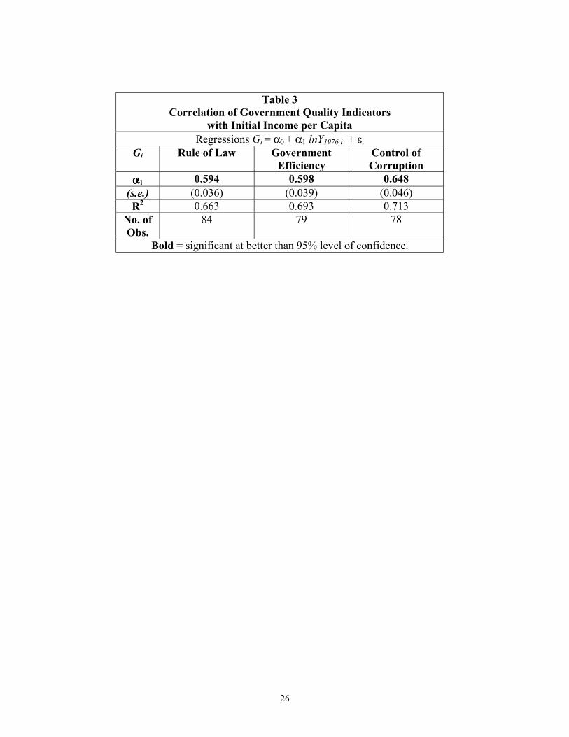
We investigate this assumption using our indicators of Rule of Law, Government

Efficiency and Control of Corruption. Table 3 presents the coefficients α1 from the

regressions

(3) Gi = α0 + α1 lnY1976,i + εi

where Gi is the indicator for either Rule of Law, Government Efficiency or Control of

Corruption for country i. The results in this table indicate that lnY1976,i is very

significantly correlated with each of these indicators of government quality since, in all

three cases, the p-value is smaller than 0.001. Furthermore, the R2 statistic for each of

these regressions is about 0.7.

A natural follow-up to specification (1), therefore, is to run three sets of

regressions, each of which takes the form

(4) ΔlnY1976-1995,i = θ0 Z*i′′′′ + θ1 Ki + θ2 (Ki x Gi ) + θ3 (Ki x Gi 2 ) + εi

where Gi is either Rule of Law, Government Efficiency or Control of Corruption for

country i, and Z*i an n x 8 matrix (n = 78 to 84 for regressions using Share76-95 and n =

53 for regressions using KQuinn) that includes both the regressors in Zi described above

and Gi. This specification is somewhat less compelling than (1) because income per

capita is correlated with a range of aspects of government quality and each of the three

18

versions of (4) includes only one measure of government quality. Nevertheless,

considering regressions of the type specified in (4) for different indicators of government

quality provides a good robustness test of the results presented in Table 1.

Table 4 presents the results of six regressions that employ specification (4), one

for each of the three measures of Gi (Rule of Law, Government Efficiency and Control of

Corruption) paired with one of the measures of Ki (Share76-95 and KQuinn). As with

Tables 1 and 2, Table 4 presents an evaluation of the partial derivative of growth with

respect to the capital account indicator evaluated at the 25th, 50th, 75th and 90th percentile

values for the respective samples. In this case, we call this partial derivative Ti where

(5) Ti = θ1 + θ2 Gi + θ3 Gi 2.

Figures 3 through 8, corresponding to the results in Columns 1 through 6 of Table 4,

respectively, present depictions of Ti for all values of Gi in the relevant range.

The results presented in Table 4, along with their depictions in Figures 3 through

8, show inverted-U shaped relationships between the responsiveness of growth to capital

account openness, Ti, and indicators of government quality. As with the estimates

depicted in Figures 1 and 2, these estimates show a range of countries in the middle of the

spectrum for which capital account openness significantly promotes economic growth. In

two cases, the estimates that interact KQuinn with Rule of Law (Column 2 and Figure 4)

and the estimates that interact KQuinn with Control of Corruption (Column 6 and Figure

8), 57 percent of the countries in the sample have an estimated Ti that is positive and

significant. The estimate of Ti based on the regression that includes an interaction of

Share76-95 with Control of Corruption (Column 5 and Figure 7) is positive and significant

19

for 36 percent of the countries in the sample. The other four regressions include about 20

percent of the sample for which Ti is positive and significant.

Quantitative assessments of the estimated impact of capital account openness on

growth can be obtained by considering the effect on ΔlnY1976-1995 of a change in the value

of the capital account indicator from its median value to its 75th percentile value (a

change in Share76-95 of 0.25 and a change in KQuinn of 0.5) for particular values of the

indicators of government reputation, analogous to the exercise performed earlier. We

calculate the estimated effect of these changes for a country at the 75th percentile of the

indicators of government reputation. The estimated changes in ΔlnY1976-1995 based on

regressions using Share76-95 and Rule of Law, Government Effectiveness and Control of

Corruption are 0.35, 0.38, and 0.60, respectively. A similar exercise based on regressions

interacting KQuinn with Rule of Law, Government Effectiveness and Control of

Corruption gives estimated changes in ΔlnY1976-1995 of 0.30, 0.25, and 0.31, respectively.

Recall that the median value of ΔlnY1976-1995 is 0.85 in the samples of the regressions

using Share76-95 and 1.29 in the samples of the regressions using KQuinn and that the

changes presented above for estimates that interact capital account openness with lnY1976

are 0.20 with the Share76-95 estimate and 0.11 with the KQuinn estimate . Thus, on a

quantitative basis, these estimates are even more striking than those based on the results

presented in Table 1.

20

V. Conclusion

This paper offers robust empirical evidence that capital account openness

contributes in an important way to economic growth for middle-income countries. The

results presented in this paper answer, to some extent, the concern voiced by Bhagwati

and others that the beneficial effects of capital account liberalization have been asserted

rather than demonstrated.

But a more nuanced view, one that growth among poorer countries may not be

promoted by capital account liberalization, is also consistent with the results presented in

this paper. The advantage of the method undertaken in this paper is that it allows for

differences across countries in the response of growth to open capital accounts depending

upon the level of income or the quality of government. Thus, this enables us to address

arguments implicit in the views presented in the introduction, including the IMF (2000)

report that recognizes a “need to carefully manage and sequence liberalization,” the claim

by Rogoff (2002) that there is widespread agreement for an “eclectic approach to capital

account liberalization” and the concerns voiced by Rodrik (1999) about the need for

“appropriate controls, regulatory apparatus and macroeconomic frameworks” in order for

a country to enjoy the benefits of capital account liberalization. The results presented

here offer evidence that, in fact, capital account openness can be a tonic but, like all

treatments, its potential for success cannot be separated from the context in which it is

administered.

21

References Arteta, Carlos, Barry Eichengreen and Charles Wyplosz, 2001, “On the Growth Effects

of Capital Account Liberalization,” (unpublished; Berkeley, California: University of California).

Bhagwati, Jagdish, 1998, “The Capital Myth: The Difference Between Trade in Widgets

and Trade in Dollars,” Foreign Affairs, Vol. 77, pp. 7–12. Edison, Hali, Michael W. Klein, Luca Ricci and Torsten Slok, 2002, “Capital Account

Liberalization and Economic Growth: Survey and Synthesis,” mimeo, December. Edwards, Sebastian, 2001, “Capital Mobility and Economic Performance: Are Emerging

Economies Different?” NBER Working Paper No. 8076 (Cambridge, Massachusetts: National Bureau of Economic Research).

Grilli, Vittorio, and Gian Maria Milesi-Ferretti, 1995, “Economic Effects and Structural

Determinants of Capital Controls,” IMF Staff Papers, Vol. 42, No. 3, pp. 517–51. Jeanne, Olivier and Pierre-Olivier Gournichas, 2002, “On the Benefits of Capital Account

Liberalization for Emerging Economies,” International Monetary Fund, mimeo. Kaufmann, Daniel, Aart Kraay and Pablo Zoido-Lobaton (2002). “Governance Matters

II: Updated Indicators for 2000-01,” World Bank Policy Research Department, mimeo.

Klein, Michael W., and Giovanni Olivei, 1999, “Capital Account Liberalization,

Financial Depth and Economic Growth,” N.B.E.R. Working Paper no. 7384, October.

Kraay, Aart, 1998, “In Search of the Macroeconomic Effects of Capital Account

Liberalization,” mimeo, The World Bank, Washington, D.C.. Available at http://econ.worldbank.org/view.php?type=5&id=22237.

Obstfeld, Maurice, 1994, “Risk-Taking, Global Diversification and Growth,” American

Economic Review, vol. 84, no. 5, (December), pp. 1310 – 1329. Quinn, Dennis, 1997, “The Correlates of Change in International Financial Regulation,”

American Political Science Review, Vol. 91, No. 3, (September), pp. 531–51. Rodrik, Dani, 1998, “Who Needs Capital-Account Convertibility?” in Stanley Fischer, et

al., Should the IMF Pursue Capital Account Convertibility? Essays in International Finance, No. 207, International Finance Section, Department of Economics, Princeton University, Princeton, N.J., (May).

22

Rodrik, Dani, 1999, The New Global Economy and Developing Countries: Making Openness Work, Overseas Development Council, Policy Essay no. 24, Washington, D.C., distributed by the Johns Hopkins University Press, Baltimore, Maryland.

Rogoff, Kenneth S., 2002, “Rethinking Capital Controls: When should we keep an open

mind?,” Finance and Development, December, pp. 55 – 56. Skidelsky, Robert, John Maynard Keynes: The Economist as Saviour, 1920 – 1937,

Macmillan, London, c. 1992.

23

Table 1 Growth Regressions with

Capital Account Openness Measures Cap. Account

Open. Indicator Share76-95 KQuinn

Reg. Number 1 2 3 4 lnY1976,i -0.053 -0.228 -0.212 -0.519

(s.e.) (0.103) (0.132) (0.185) (0.251) ln(School) 0.035 0.036 0.042 0.049

(s.e.) (0.091) (0.105) (0.138) (0.154) InvestAv’g 74 - 78 0.027 0.033 0.042 0.039

(s.e.) (0.010) (0.012) (0.014) (0.017) Pop.Growth -1.153 -0.934 -1.804 -1.695

(s.e.) (0.487) (0.687) (0.537) (0.664) Africa -0.327 -0.628 -0.519 -0.644 (s.e.) (0.184) (0.258) (0.271) (0.272)

Ki -26.624 -60.981 -2.936 -5.541 (s.e.) (10.769) (20.256) (2.484) (3.021)

(Ki x lnY1976,i ) 7.053 15.340 0.808 1.366 (s.e.) (2.768) (5.286) (0.585) (0.707)

(Ki x lnY1976,i 2 ) -0.453 -0.942 -0.052 -0.079 (s.e.) (0.176) (0.342) (0.034) (0.042)

Evaluating Overall Effect, Bi, for i at listed percentiles of lnY1976 25th Percentile -1.102 -3.212 0.110 -0.071

(s.e.) (0.704) (1.205) (0.148) (0.240) 50h Percentile 0.129 -0.623 0.192 0.154

(s.e.) (0.242) (0.626) (0.076) (0.127) 75th Percentile 0.798 1.459 0.211 0.333

(s.e.) (0.202) (0.462) (0.098) (0.105) 90th Percentile 0.287 1.020 0.159 0.329

(s.e.) (0.158) (0.621) (0.116) (0.149) # w/sig. + effect

percentiles 26

58th – 88th 16

67th – 86th 15

49th – 75th 21

55th – 94th R2 0.583 0.519 0.579 0.594

no. of obs. 85 79 53 51 Est. Method OLS IV OLS IV

Bold = significant at better than 95% level of confidence, Italic = significant at 90% - 95% level of confidence.

24

Bi and ln(GDP per Capita, 1976)

B, V

alue

of L

inea

r Com

bina

tion

of C

oeffi

cien

ts

FIgure 1, Share, Quadratic Interaction w/GDP per capitaln(GDP per Capita), 1976

Effect of Share on Growth Lower Bound, 95% Conf. Interval Upper Bound, 95% Conf. Interval

4.5 5.05 6.79 7.78 8.82 9.19

-2.54

0.31.8

B, V

alue

of L

inea

r Com

bina

tion

of C

oeffi

cien

ts

Figure 2, KQuinn, Quadratic Interaction w/GDPln(GDP per Capita), 1976

Cap.Acc't Effect on Growth Lower Bound, 95% Conf. Interval Upper Bound, 95% Conf. Interval

4.98 6.88 7.82 8.39 9.19

0

.18

.22

25

Table 2: Growth Regressions with Capital Account Openness Measures and Indictors of Government Quality Cap. Account

Open. Indicator Share76-95 KQuinn

Reg. Number 1 2 3 4 lnY1976,i -0.198 -0.240 -0.202 -0.328

(s.e.) (0.099) (0.125) (0.160) (0.225) ln(School) 0.011 0.012 0.049 -0.031

(s.e.) (0.112) (0.123) (0.157) (0.155) InvestAv’g 74 - 78 0.019 0.021 0.025 0.019

(s.e.) (0.010) (0.012) (0.012) (0.015) Pop.Growth -0.819 -0.734 -1.550 -1.653

(s.e.) (0.515) (0.664) (0.496) (0.615) Africa -0.407 -0.571 -0.771 -0.915 (s.e.) (0.187) (0.225) (0.225) (0.244)

Rule of Law 0.346 0.326 0.220 0.292 (s.e.) (0.139) (0.154) (0.199) (0.224)

Gov. Efficiency 0.139 0.062 0.064 -0.047 (s.e.) (0.184) (0.210) (0.218) (0.249)

Corrupt. Cntrl -0.071 -0.088 0.074 0.071 (s.e.) (0.173) (0.177) (0.219) (0.226)

Ki -19.520 -42.705 -1.849 -3.288 (s.e.) (7.417) (18.237) (2.309) (2.887)

(Ki x lnY1976,i ) 5.266 11.005 0.579 0.927 (s.e.) (1.931) (4.776) (0.543) (0.668)

(Ki x lnY1976,i 2 ) -0.345 -0.692 -0.041 -0.061 (s.e.) (0.124) (0.309) (0.031) (0.039)

Evaluating Overall Effect, Bi, for i at listed percentiles of lnY1976 25th Percentile -0.401 -1.384 0.166 0.133

(s.e.) (0.370) (0.890) (0.137) (0.251) 50th Percentile 0.241 -0.065 0.185 0.212

(s.e.) (0.181) (0.539) (0.074) (0.141) 75th Percentile 0.552 1.022 0.118 0.186

(s.e.) (0.184) (0.453) (0.099) (0.105) 90th Percentile 0.087 0.463 0.036 0.117

(s.e.) (0.169) (0.562) (0.117) (0.151) # w/sig. + effect

percentiles 23

56th – 84th 10

68th – 81st 8

45th – 58th 7

63rd – 72nd R2 0.661 0.644 0.638 0.594

no. of obs. 78 73 53 51 Est. Method OLS IV OLS IV

Bold = significant at better than 95% level of confidence, Italic = significant at 90% - 95% level of confidence.

26

Table 3 Correlation of Government Quality Indicators

with Initial Income per Capita Regressions Gi = α0 + α1 lnY1976,i + εi

Gi Rule of Law Government Efficiency

Control of Corruption

αααα1 0.594 0.598 0.648 (s.e.) (0.036) (0.039) (0.046) R2 0.663 0.693 0.713

No. of Obs.

84 79 78

Bold = significant at better than 95% level of confidence.

27

Table 4

Growth Regressions with Capital Account Openness Measures Interacted with Indictors of Government Quality

Measure of Gi Rule of Law Government Efficiency Control of Corruption Measure of Ki Share KQuinn Share KQuinn Share KQuinn

lnY1976,i -0.217 -0.227 -0.239 -0.272 -0.207 -0.249 (s.e.) (0.092) (0.128) (0.100) (0.128) (0.094) (0.115)

ln(School) 0.006 -0.132 0.030 0.016 -0.036 -0.081 (s.e.) (0.094) (0.193) (0.108) (0.136) (0.111) (0.135)

InvestAv’g 74 - 78 0.022 0.037 0.030 0.040 0.030 0.040 (s.e.) (0.010) (0.014) (0.010) 0.015 (0.101) (0.014)

Pop.Growth -0.941 -1.555 -0.968 -1.497 -0.803 -1.260 (s.e.) (0.445) (0.469) (0.520) (0.511) (0.534) (0.494)

Africa -.401 -0.633 -0.408 -0.542 -0.510 -0.586 (s.e.) (0.167) (0.259) (0.189) (0.245) (0.194) (0.237)

Gi 0.387 0.199 0.366 0.193 0.365 0.262 (s.e.) (0.112) (0.204) (0.100) (0.276) (0.119) (0.194)

Ki -0.013 -0.013 -1.652 -0.060 -1.081 0.012 (s.e.) (0.510) (0.183) (0.990) (0.307) (0.625) (0.152)

(Ki x Gi ) 0.446 0.212 1.621 0.221 1.584 0.290 (s.e.) (0.482) (0.138) (0.766) (0.225) (0.497) (0.106)

(Ki x Gi 2 ) -0.124 -0.045 -0.316 -0.047 -0.365 -0.082 (s.e.) (0.122) (0.026) (0.142) (0.034) (0.599) (0.020)

Evaluating Overall Effect, Bi, for i at listed percentiles of Gi 25th Percentile 0.249 0.171 -0.128 0.142 0.218 0.190

(s.e.) (0.290) (0.100) (0.315) (0.112) (0.276) (0.095) 50h Percentile 0.358 0.235 0.218 0.196 0.483 0.247

(s.e.) (0.217) (0.089) (0.200) (0.089) (0.217) (0.075) 75th Percentile 0.350 0.227 0.431 0.195 0.573 0.234

(s.e.) (0.166) (0.094) (0.180) (0.114) (0.159) (0.076) 90th Percentile 0.224 0.203 0.261 0.174 0.090 0.118

(s.e.) (0.202) (0.101) (0.183) (0.128) (0.183) (0.104) # w/sig. + effect

percentiles 18

60th – 80th 31

32nd – 89th 18

61st – 82nd 13

43rd – 66th 29

49th – 85th 31

30th – 87th R2 0.638 0.609 0.619 0.610 0.618 0.652

no. of obs. 84 53 79 53 78 53 Estimation by OLS, with robust standard errors.

Bold = significant at better than 95% level of confidence, Italic = significant at 90% - 95% level of confidence.

28

Ti and Rule of Law

T, V

alue

of L

inea

r Com

bina

tion

of C

oeffi

cien

ts

Figure 3, Share, Quadratic Interaction with Rule of LawRule of Law

Effect of Share on Growth Lower Bound, 95% Conf. Interval Upper Bound, 95% Conf. Interval

0 1.69 2.48 3.29

0

.33

.39

T, V

alue

of L

inea

r Com

bina

tion

of C

oeffi

cien

ts

Figure 4, KQuinn, Quadratic Interaction with Rule of LawRule of Law

Effect of KQuinn on Growth Lower Bound, 95% Conf. Interval Upper Bound, 95% Conf. Interval

0 1.35 2.36 3.23 3.5

0

.19

.24

29

Ti and Government Efficiency

T,

Val

ue o

f Lin

ear C

ombi

natio

n of

Coe

ffici

ents

FIgure 5, Share, Quad. Int. with Government EfficiencyGovernment Efficiency

Effect of Share on Growth Lower Bound, 95% Conf. Interval Upper Bound, 95% Conf. Interval

0 2.09 2.57 3.05 3.78

0

.36.43

T, V

alue

of L

inea

r Com

bina

tion

of C

oeffi

cien

ts

Figure 6, KQuinn, Quad. Interaction w/Gov't. EfficiencyGovernment Efficiency

Effect of KQuinn on Growth Lower Bound, 95% Conf. Interval Upper Bound, 95% Conf. Interval

0 1.66 2.37 3.54

0

.17.2

30

Ti and Control of Corruption

T, V

alue

of L

inea

r Com

bina

tion

of C

oeffi

cien

ts

Figure 7, Share, Quadratic Interaction w/Control of CorruptionControl of Corruption

Effect of Share on Growth Lower Bound, 95% Conf. Interval Upper Bound, 95% Conf. Interval

0 1.45 2.17 3.12 3.696

0

.31

.45

.64

T, V

alue

of L

inea

r Com

bina

tion

of C

oeffi

cien

ts

Figure 8, KQuinn, Quad. Int. w/Control of CorruptionControl of Corruption

Effect of KQuinn on Growth Lower Bound, 95% Conf. Interval Upper Bound, 95% Conf. Interval

0 .8 1.77 2.8 3.225

0

.18

.27