NBER WORKING PAPER SERIES

CHOOSING ELECTORAL RULES:THEORY AND EVIDENCE FROM US CITIES

Philippe AghionAlberto Alesina

Francesco Trebbi

Working Paper 11236http://www.nber.org/papers/w11236

NATIONAL BUREAU OF ECONOMIC RESEARCH1050 Massachusetts Avenue

Cambridge, MA 02138March 2005

We thank Matilde Bombardini, Gary Chamberlain, John Friedman, Edward Glaeser, Richard Holden,Caroline Hoxby, David Lucca, James Robinson, and John Wallis for useful comments and suggestions. Weare grateful to participants of the CIAR meetings in Toronto and seminars at Harvard University. DilyanDonchev, Laura Serban, and Radu Tatucu provided excellent research assistance. Trebbi acknowledgesfinancial support from the Social Sciences Research Council. The views expressed herein are those of theauthor(s) and do not necessarily reflect the views of the National Bureau of Economic Research.

©2005 by Philppe Aghion, Alberto Alesina, and Francesco Trebbi. All rights reserved. Short sections oftext, not to exceed two paragraphs, may be quoted without explicit permission provided that full credit,including © notice, is given to the source.

Choosing Electoral Rules: Theory and Evidence from US CitiesPhilppe Aghion, Alberto Alesina, and Francesco TrebbiNBER Working Paper No. 11236March 2005JEL No. H0

ABSTRACT

This paper studies the choice of electoral rules, in particular, the question of minority representation.

Majorities tend to disenfranchise minorities through strategic manipulation of electoral rules. With

the aim of explaining changes in electoral rules adopted by US cities (particularly in the South), we

show why majorities tend to adopt "winner-take-all" city-wide rules (at-large elections) in response

to an increase in the size of the minority when the minority they are facing is relatively small. In this

case, for the majority it is more effective to leverage on its sheer size instead of risking to concede

representation to voters from minority-elected districts. However, as the minority becomes larger

(closer to a fifty-fifty split), the possibility of losing the whole city induces the majority to prefer

minority votes to be confined in minority-packed districts. Single-member district rules serve this

purpose. We show empirical results consistent with these implications of the model.

Philippe AghionDepartment of EconomicsUniversity College LondonGower StreetLondon, WC1 6BTand NBERp_aghion@harvard.edu

Alberto AlesinaDepartment of EconomicsHarvard UniversityCambridge, MA 02138and NBERaalesina@harvard.edu

Francesco TrebbiDepartment of EconomicsHarvard UniversityCambridge, MA 02138trebbi@fas.harvard.edu

1 Introduction

One of the key questions in political economy is how different electoral laws affect

policy outcomes. In order to provide an answer several authors take electoral

rules as exogenous or predetermined and use them as explanatory variables for

various policies1 . However, the rules of government are themselves endogenous

variables chosen at constitutional tables. Ideally, rules should be chosen behind

a ”veil of ignorance”, that is decisions should be taken as if one ignored the

identity of those benefiting from the choices themselves. In reality, however, in

most constitutional tables the veil of ignorance is ”see-through”, in the sense

that there is some knowledge of who would benefit under alternative rules and

of what policy outcomes those rules would produce. Therefore the ”exogeneity”

of constitutions can be called into question.

Our focus is on the question of minority representation, with special refer-

ence to the nature of electoral districts and alternative rules for the choice of

representatives. We have two goals in mind, one more general and one more

specific. The first and more general point is to make progress in modeling in-

stitutional choice as endogenous. On the first point, most of the literature is

normative, i.e. it discusses how electoral laws should be chosen, starting from

the work of Hayek (1960) and Buchanan and Tullock (1962)2. A normative

approach usually characterizes works in Political Science, with some notable ex-

ception such as Riker (1986) and several essays in Colomer (2004).Economists

have only recently began to pay attention to the endogeneity of political insti-

1A classic study is Lijphart (1994). The most recent contributions on the effects of insti-

tutions (taken as exogenous or prestermined) on economic policies are Persson and Tabellini

(2003) for a sample of democratic countries and Baqir (2003) for a cross-section of US cities.

They build upon a vast literature on the effects of alternative forms of government on policies,

a literature that we do not review here. We refer the reader to Persson and Tabellini (2003) for

a survey of the cross-country literature. On US states see in particular Alt and Lowry (1994),

Poterba (1994), and Bohn and Inman (1996) amongst others. Mulligan and Sala I Martin

(2004) offer a dissenting view, namely that policies are determined by lobbying pressure that

are not much affected by institutional forms of government.2For a survey of the literature on Constitutional Theory, see Voigt (1997).

2

tutions from a positive, as opposed to a normative perspective. Alesina and

Glaeser (2004) for instance discuss how the choice of alternative electoral rules,

which are themselves associated with different policy choices over the welfare

state, are indeed the result of strategic constitutional choices. The present pa-

per is a study in ”positive constitutional theory”, with a special emphasis on

the question of how majorities select electoral rules to partially disenfranchise

minorities.

The second and more specific goal of our paper is to analyze the evolution

of minority representation in American cities. We examine empirical evidence

drawn from US municipalities, that adopt two types of electoral rules: either a

single-member district (also called single-district) or at-large rules (or a com-

bination of the two). Councilmen elected by district compete for one or, more

rarely, multiple seats in each geographic subdivision (district or ward) of the

city. Differently, in at-large elections, officials are elected in multi-member plu-

rality districts, voters have as many votes as there are council seats, and the

only multi-member district is identified by the city itself. The basic ”winner-

take-all” logic holds for both rules. For given council size, the difference between

single-district and at-large rules is due to geographic clustering of groups of vot-

ers with homogeneous preferences3. We show why majorities at the constitution

design stage tend to adopt at-large electoral rules in response to an increase in

the size of the minority when the minority they are facing is relatively small.

In this case, as the size of the minority increases, for the majority it becomes

more effective to leverage on its sheer size instead of risking to concede repre-

sentation to voters from minority-elected districts. However, as the minority

becomes larger (closer to a fifty-fifty split), the possibility of losing the whole

city induces the majority to prefer minority votes to be confined in minority-

packed districts. Single-member district electoral rules serve this purpose. This

shift in the preferences of the (constitutional) majority, first towards an at-large

3See Cutler, Glaeser, and Vigdor (1999) for a detailed account of racial segregation patterns

in the United States. The assumption of geographic clustering will be maintained throughout

the paper.

3

electoral rule, and then towards a single-district rule as the size of the minority

increases, is precisely what the data show.

When discussing local politics in the US, one is immediately thrown into the

area of race relations.4 In fact, it is quite compelling to identify the ”majority”

with the whites and the ”minority” with racial ”minorities” (perfect choice of

words!). The evolution of voting rights, especially in the South, allows us to

test implications of the model regarding the endogenous institutional choice.

Until the mid-sixties, before the civil right movement and the Voting Rights

Act of 1965, racial minorities (mainly blacks) in the South were essentially

disenfranchised by a battery of regulations that, although color-blind on paper,

were in practice directed to severely limit black vote. In this context the choice

of electoral rules and forms of governments had not much to do with a white

majorities’ attempt at controlling black influence on city governments, since

blacks did not vote. After the mid-sixties, due to novel federal Voting Rights

legislation, black influence increased substantially in terms of their ability to

elect representatives. Indeed, after the Voting Rights Act of 1965, we show that

decisions about electoral rules reflected changes in the relative size of the white

and black populations in a way consistent with our model.

Manipulation of electoral rules is not a prerogative exclusive of American

cities. Alexander (2005, p.211) describes in detail the 1947 Gaullist manipula-

tions of electoral rules in France. In the Paris area where the Gaullist alliance

was weak they introduced proportional representation, in rural areas where the

alliance was strong, they introduced plurality rule. Krenzer (2005, p.229) de-

scribes strategic manipulation in Germany. One could go on.

Our empirical results on (within-)US cities variation are quite consistent

with previous findings on the cross-country evidence in Alesina, Aghion, and

Trebbi (2004). In both cases constitutional choices do not seem to occur behind

4For discussion of the importance of race in American local politics, see for instance Hacker

(1992), Huckfeld and Kohfeld (1989) and Wilson (1996) amongst many others. Alesina, Baqir,

and Hoxby (2004) argue that even the design and number of local jurisdictions in the US

depends upon race relations.

4

a veil of ignorance in the sense that, as the minority increases its size and/or its

political rights, the majority tries to make constitutional changes that limit the

protection of minorities, while behind a veil of ignorance exactly the opposite

should happen (as one would take into account the likelihood of belonging to a

minority).

The paper is organized as follows. Section 2 illustrates the model. Section

3 describes the institutional context of US city government to which the model

is applied and our data. Section 4 illustrates our empirical results. The last

section concludes.

2 The model

The structure of the model is as follows. There are two groups of voters, whites

(W ) and blacks (B). We denote the initial relative size of group B as π > 0, so

that the size of group W is (1−π). The whites are, initially at least, a majority

(we restrict π < 1/2) and they are those who choose the electoral rule for the

city (in short, we call the choice of the electoral rule: "constitution"). This is

because either the blacks are disenfranchised at the time of the constitutional

choice or they were outvoted at the constitutional table. The white choose

a constitution with an eye on maximizing their expected utility arising from

a policy outcome which will be decided by an elected council. In order to

make the problem interesting there is uncertainty in the relative share of the W

and B voters, so that the constitutional writers cannot be sure ex ante of the

composition of the council. In other words, there is a shock to the composition

of the electorate between the writing of the constitution and the choice of the

policy. Moreover, the composition of the council depends on the electoral rule

chosen. This modeling strategy builds upon the incomplete social contracts

ideas of Aghion and Bolton (2003). We now present the model more formally.

5

2.1 Agents and expected utility

We first present a basic version of the model. We discuss extensions later. The

population is equally spread over three electoral districts, numbered 1, 2, 3, and

with M individuals in each. Each district chooses a seat in the council. The

initial number of B and W voters in each district are given by Bi and Wi for

i = 1, 2, 3. We assume that:

W1 = M ;

W2 = W3 = (1

2+ z)M,

where z is a real number between −1/4 and 1/2. In other words, the parameterz will allow us to make comparative statics on the initial number of B voters in

districts 2 and 3. Note that this range of variation for z insures that 0 < π < 1/2.

Thus, z parametrizes the size of the ex ante W majority. Indeed, we have:Xi

Wi = (2 + 2z)M = 3(1− π)M,

therefore:

z =1− 3π2

. (1)

Thus, initially theW voters have a majority and they can choose the electoral

rule (constitution). Given the electoral rule, a three-member council is elected.

The council decides the policy. After the constitution is chosen, there is a shock

to the composition of voters in the city, to which the electoral rule cannot be

made contingent upon.

More formally, we suppose that during the interim phase an exogenously

given mass LN of new B voters joins the polity5 , with LN = αM where α is a

random variable uniformly distributed between 0 and an upper bound α ∈ (1, 2).Moreover, we assume that the newcomers are not evenly distributed across the

5One could assume that mobility across cities is affected by the nature of charter rules,

electoral systems, and the identity of the mayor, an issue which we do not tackle in the model.

See Epple and Romer (1991) for a classic treatment of endogenous mobility in a political

economy model. However, empirical evidence of Tiebout sorting is scant. See Strumpf and

Oberholzer-Gee (2002). We discuss this effect in Section 4.

6

three districts, but that instead one half of them joins district 2, whereas the

remaining half goes to district 3 (thus, no new B voter enters district 1).

Different compositions of the council imply different policies. We assume

that with no W representative and three B representatives the implemented

policy is most unfavorable to the W group which obtains a low utility level r.

With one W representative the W group ends up with the status quo utility

level u0; with two or three representatives the W group achieves its maximum

utility level r. (Think of r as being the result of the B group’s most favorable

policy being implemented, and of r as being the outcome of theW group’s most

favorable policy).

This last assumption is twofold. First, note that the W group is advan-

taged: with two W councilmen the W bliss point obtains and with only one

W councilman the status quo obtains. This may capture either one of two

empirical features, or both. One is some inherent advantage of W ; another,

more interestingly, may capture the functioning of a council in the presence of

a W mayor. For the moment we are ignoring the role of the mayor and the

specifics of the form of government, but we will return to this below. Second,

the assumption implies that the size of the B majority matters for the policy

outcome; a two-one B majority implies a different policy from a three-zero B

majority6. In any event the specifics of the policy outcome formulation do not

affect the qualitative nature of the results, as we discuss below.

The ex ante expected utility of a W constitution writer is then equal to:

Uw = (1− p0 − p1)r + p1u0 + p0r,

where pj denotes the probability that j council representatives belong to the

W− group at the interim stage. The choice of electoral rules (the constitution)

chosen by the W voters will determine the value of p0 and p1.

Summarizing, the timing of events is as follows:

1. Electoral rules are chosen by the W group.6See Alesina and Rosenthal (1995) for an extensive discussion of this assumption and a

comparison with alternatives.

7

2. The interim distribution of preferences is realized, which translates into a

majority of the council.

3. Payoffs realize.

2.2 Electoral rules and ex ante expected utilities

With an eye to the case of American cities, we now study two alternative elec-

toral rules. The first one, referred to as representation "at-large" (AL), allocates

all seats to the party that wins more than fifty percent of the votes. The sec-

ond rule, referred to as ”single-member district rule” (SD), requires that each

candidate runs in a particular district and obtains a majority of votes within

the district in order to be elected.

Given our above assumptions as to the group composition of the three dis-

tricts, we immediately have that p1 = 0 under the AL rule, whereas p0 = 0

under the SD rule. We now compute the expected ex ante utilities of constitu-

tion writers in the W− group, respectively under these two electoral rules.

2.2.1 Expected utility under the at-large rule

Under the AL rule all council seats will go to the B group if and only if:

B1 +B2 +B3 + LN > W1 +W2 +W3.

Then, the ex ante expected utility of constitution writers in the W− group canbe simply expressed as

UALW = p0r + (1− p0)r = r − p0∆,

where ∆ = r − r is the constitution writers’ loss from losing the majority, and

p0 = Pr(B1 +B2 +B3 + LN > W1 +W2 +W3) = Pr(α > 1 + 4z)

is the probability of losing the majority. Substituting for z as a function of π

using (1), we have:

p0 = max

µ1− 3

α(1− 2π), 0

¶, (2)

8

so that the ex ante expected loss of constitution writers in the W− group underthe AL rule, is equal to:

LALW = p0∆ = (1−3

α(1− 2π))+∆,

where we use the notation

x+ = max{x, 0}.

2.2.2 Ex ante expected utility under the single-member district rule

Under the SD rule council seats are allocated at the district level. The probabil-

ity of the B− group winning a majority of two seats is equal to the probabilitythat districts 2 and 3 be won by the B group. Given that the same fraction of

new B voters are allocated to these two districts, which already start with the

same fraction of B voters ex ante, and given that there is a fixed majority of W

voters in district 1, we immediately get that the B− group obtains a two-seatmajority with probability:

p1 = Pr(B3 +1

2αM > W3) = p1 = Pr(α > 4z)

or, after substituting for z using (1):

p1 = (1−2

α(1− 3π)+)+. (3)

We can then re-express the ex ante utility of constitution writers in the W−group under the SD rule, as:

USDW = p1u0 + (1− p1)r = r − p1δ,

where δ = r − u0 is the constitution writers’ loss from losing the majority, and

therefore

LSDW = p1δ = (1−1

α(1− f)(1− 3π)+)+δ,

is the expected loss of constitution writers in the W− group under the SD rule.

9

2.3 The size of minorities and the choice of electoral rule

Ex ante at the constitutional stage, individuals in the W− group will simplychoose the electoral rule that minimizes the expected loss LW . Our main the-

oretical prediction can be summarized intuitively as follows. If initially the W

group commands a very large majority of votes, the constitution writers do not

fear they can lose the majority under either rule, thus they are indifferent be-

tween the two rules. As the relative size of the B−group increases, however,at some point it becomes preferable for constitution writers in the W−groupto move to AL in order to reduce the power of the B− voters in districts 2,

3 by confronting them with the whole pool of W− voters, including those indistrict 1. Doing so allows the W−group to preserve its majority as long asthe fraction of B−individuals does not become too large. Finally, when thefraction of B−voters becomes sufficiently large that it becomes impossible toprevent their becoming the new majority, moving back to the SD rule allows

the W−group to limit their losses: indeed, as π becomes sufficiently close to1/2 , the risk of losing all three districts and of thereby incurring the large loss

∆, makes the W−group prefer a SD system which guarantees them at least

1 seat in the council -and thereby limits their loss to δ << ∆- given that in

this case B−voters are restricted to commanding districts 2 and 3 only. Notsurprisingly, this latter motive from moving back from AL to SD disappears if

the loss incurred by the minority is independent of the size of the majority, that

is if ∆ = δ.

More formally, we can state:

Proposition 1 (a) Both rules AL and SD involve no utility loss to W−groupindividuals when π ∈ (0, 13 −

α6 ); (b) if

∆δ > (1− 1

α)−1, then there exists a unique

cut-off point bπ ∈ ( 13 − α6 ,

13) such that

LALW < LSDW if π ∈ (13− α

6, bπ)

and

LALW > LSDW if π ∈ (bπ, 12);

10

(c) if ∆ = δ, then for all π ∈ (13 −α6 ,

12) the AL rule dominates the SD rule.

Proof. Part (a) is straightforward. Part (b) follows from the fact that: (i)

we have

LALW = 0 < LSDW if π ∈ (13− α

6,1

2− α

6);

(ii) for π = 13 , we have:

LALW = (1− 1α)∆ > LSDW = δ;

(iii) LALW and LSDW are both linear increasing in π for π ∈ ( 12 −α6 ,

13); hence the

existence of a unique cut-off bπ ∈ (12 − α6 ,

13) with the desired properties. Finally,

to establish part (c), let us reason by contradiction and suppose that for some

π between 0 and 12 , we have

LSDW < LALW

or equivalently since here ∆ = δ,

(1− 2α(1− 3π)+)+ < (1− 3

α(1− 2π))+. (4)

First, this cannot be the case for π ∈ ( 13 ,12 ) since in that case (4) becomes:

1 < (1− 3α(1− 2π))+,

which is impossible if π < 1/2. Second, suppose that (4) holds for some π < 1/3.

It cannot be the case that both expressions are positive, otherwise we would have

(1− 2α(1− 3π)) < (1− 3

α(1− 2π)),

or equivalently

1− 2α< 1− 3

α

which is impossible; and it cannot be the case that

(1− 2α(1− 3π)) < 0 < (1− 3

α(1− 2π))

as this would imply that1

2− α

6<1

3− α

6,

again an impossibility. This establishes the proposition.

This proposition can be generalized to the case of N districts. We do so in

the following extensions.

11

3 Extensions

3.1 The N district case

Suppose the polity’s population is equally spread over the electoral districts, now

numbered 1, ..., N , and withM individuals in each. We maintain the assumption

that the same two types of (ex ante) districts exist:

W1 = M ;

W2 = (1

2+ z)M ;

where again W1 districts are ”all-W” while W2 districts are an identical mix of

W and B. We also maintain the assumption that district design is exogenously

given as we focus on the electoral rule for given district design. There are N1

districts like W1, therefore N2 = N − N1. For N2 < N1, it is clear that under

SD the W group cannot be blocked, no matter how large the group αM of B

voters is. We exclude this instance and focus on the more interesting case where

N2 > N1.

Now consider the blocking probabilities under AL and under SD respec-

tively. Blocking under AL will occur whenever the ex post total number of

W−voters, NM (1− π) , is larger than the ex post total number of B−voters,αM +NMπ. Thus, nothing fundamental changes from the three-districts case,

and we now have:

p0 =

µ1− N

α(1− 2π)

¶+.

Turning to the SD rule, let us first assume that each district j of the N2

districts receives a fraction 1N2of new comers, all of them belonging to the B−

group. In this case the probability that the B−group wins a majority of seatson the council, is simply equal to the probability that the B−group acquire amajority of votes in any of the W2 districts, namely

pN2 = Pr(αM

N2+ (

1

2− z)M > (

1

2+ z)M),

that is

pN2= Pr(α > 2zN2),

12

where now

z =1

2− π

N

N2.

We then obtain:

pN2 = (1−N2

α(1− 2π N

N2)+)+.

Once again, the constitution writers will choose the electoral rule that in-

volves the lowest ex ante expected loss, where

LALW = p0∆ = (1−N

α(1− 2π))+∆

and

LSDW = (1− N2

α(1− 2π N

N2)+)+δ(N2),

where it is reasonable to assume that the loss δ(N2) to the W−group if theB−group acquires majority of seats on the council, is non-decreasing in thenumber of seats N2 the B−group holds in that case.Assume

α < N2.

Then for π very close to zero, both LALW and LSDW are equal to zero, so that

constitution writers are indifferent between the two electoral rules. Next, note

that for all π < 1/2, we have

(1− N

α(1− 2π)) < (1− N2

α(1− 2π N

N2)), (5)

so that as π increases away from zero, LSDW becomes positive before LALW does;

this in turn implies that for intermediate values of π, constitution writers in

the W−group will prefer the AL rule to the SD rule, as the former dilutes the

B−votes among the whole W−population. Finally, as π becomes arbitrarilyclose to 12 , the expected loss L

ALW under AL converges to∆, whereas the expected

loss LSDW converges to (1+ N−N2

α )δ(N2). It then follows that the W−group willchoose the SD rule whenever(1 + N−N2

α )δ(N2) < ∆.

We thus obtain a straightforward generalization of Proposition 1 to the more

general case where the number of districts N is arbitrary. Note however that

13

condition (5) becomes hard to satisfy when the number N2 of W2 districts

becomes arbitrarily close to N.

3.2 Uneven distribution of newcomers

In order to gain intuition in this and the following subsections, let us return

to the three-district model employed in Section 2.1. In our analysis so far we

assumed that equal numbers of new B− group voters would choose to locatein districts 2 and 3. However, our reasoning and result extend to the case

where a fraction f > 1/2 of new comers choose say district 2 whereas the

remaining fraction (1 − f) chooses district 3. This obviously does not affect

the probability p0 of the B− group winning all seats under the AL rule sincethat probability depends only upon the overall fraction of B− individuals in theoverall population. Thus, we still have:

p0 = (1−3

α(1− 2π))+,

so that the ex ante expected loss from the AL rule, is still equal to:

LALW = (1− 3α(1− 2π))+∆.

However, the B− group will only win a majority of seats on the council if itwins a majority of votes in districts 2 and 3, which in turn requires that it win

a majority of votes in district 3, which, of the two districts, is the harder one to

win. Therefore,

p1 = Pr(B3 + (1− f)αM > W3) = Pr(α >2z

1− f).

This yields:

p1 = (1−1

α(1− f)(1− 3π)+)+

with a corresponding ex ante expected loss under SD rule equal to:

LSDW = (1− 1

α(1− f)(1− 3π)+)+δ.

Assume

α < min{3, 1

1− f}

14

so that p0 = p1 = 0 for π sufficiently small.

Then, it is easy to show that Proposition 1 continues to holds in its entirety

when

1− f ≥ 13

(6)

since in that case,

1− 3α(1− 2π) < 1− 1

α(1− f)(1− 3π)

which implies that, as π increases from zero, p1 becomes positive before p0 does.

On the other hand, one can easily show that when (6) is violated, then the AL

rule is always weakly dominated by the SD rule when ∆δ is sufficiently large.

3.3 Gerrymandering

An important practical consideration is that the design of district may itself

be endogenous. In particular, the constitution writing majority may be try to

"gerrymander" the districts in order to minimize the number of representative

elected by the minority. The possibility of unconstrained gerrymandering obvi-

ously makes the SD rule preferable to a majority writing the constitution. As we

will discuss below, empirically this is an important consideration for American

cities. How advantageous for the white majority it is to choose gerrymandering

with a SD system versus an AL system, depends also on the nature of resi-

dential segregation in the city7. This is of course a well know issue in the vast

literature on gerrymandering.8

In the context of the above model, the constitution writers in theW− groupwill simply choose to maximize f, that is, to pack as many new B−votersas possible in one district, say district 2, in order to prevent them from ever

acquiring a majority of votes in the council. In the absence of any constraints

on gerrymandering (one such constraint for example would be that differentials

7Cole (1976) for instance emphasizes how at large elections, while in principle should favor

minorities which are spread out within city boundaries, in fact do not.8On gerrymandering, see in particular Cox and Katz (2002) and Friedman and Holden

(2005).

15

between the number of voters across the various districts cannot be larger than

a given percentage), the constitution writers will simply choose f equal to one,

in which case SD will always dominates AL. However, if various constraints

on gerrymandering limits the maximum f that can be achieved by constitution

writers in the W−group, then as we just saw in the previous subsection the

conclusions of Proposition 1 will again hold as long as f < 2/3.

Finally, it is interesting to note that the possibility of gerrymandering could

give rise to the same pattern with AL dominating for intermediate values of π

and SL dominating for high values of π, even when the loss incurred by the

W−group is independent of the size of the B−majority, that is, even when∆ = δ. To see this, let us slightly modify our basic model by assuming that as

in Proposition1 by assuming that constitution writers in the W−group sufferfrom having the B−group hold even one (minority) seat in the council. Then,as the size π of the B−group increases from zero to 1/2, the W−group will firstchoose the AL rule in order to dilute the B−voters among all W−voters as inour previous analysis. But then, as π increases further, the only way to prevent

the B−group from winning a majority of seats is to move from AL to SD and

at the same time "gerrymander", that is pack all B−voters in one district.Already without gerrymandering, the SD rule already allowed theW−group

to "waste" B−votes by preventing them from contaminating district 1. With

gerrymandering the wasting (or packing) effect of SD is only reinforced: B−voterscannot outnumber W−voters now in two districts instead of one in the absenceof gerrymandering. But the logic and predictions are basically the same with

and without gerrymandering.

3.4 Uniform distributions of voters across districts

Suppose the three districts are evenly affected by any ex ante variation in the

size of the B population, namely:

Wi =1

2+ z, for i = 1, 2, 3,

16

we have

z =1

2− π,

and that new comers are also evenly distributed across the three districts. Then

the probabilities of the B−group winning under the AL and SD rules, are the

same and equal to:

p0 = (1−3

α(1− 2π))+,

and the ex ante expected loss of constitution writers under the two rules are

also the same equal to

L = p0∆.

This underlies the importance of the unevenness of the distribution of B

within the electoral area (the city) if we want to explain why local constitutions

shift from one rule to another as the relative influence of B− voters increases.In particular, the well known pattern of segregation in American cities makes

this uniform distribution case not relevant.

Now, suppose that while ex ante B−voters are evenly distributed across thethree districts, ex post new comers migrate only to districts 2 and 3. In that

case, the probability of the B−group winning under the AL rule is still equalto p0, whereas their probability of winning under the SD rule is now given by

p1 = (1−2

α(1− 2π))+.

But then it is easy to see that constitution writers in the W− group will neverprefer the SD rule for values of π close to 1

2 since

LSDW (π =1

2) = p1δ = δ < LALW (π =

1

2) = p0∆ = ∆.

Given that

(1− 3α(1− 2π)) < (1− 2

α(1− 2π)),

for all π, as before as π increases away from zero, the ex ante expected loss

LSDW will become positive before LALW does. Overall, as π increases from 0 to

1/2, constitution writers will first be indifferent between the two rules, then

17

will prefer the AL rule because it dilutes B−votes, then may prefer the SD rule

because it reduces losses, but then eventually will always reverse to the AL rule.

As we shall see in the empirical analysis, this last reversal to the AL rule (which

is the one departure from Proposition 1) is not observed in our cross-city data.

3.5 Mayors and managers

Another dimension that differentiates between American cities, is the degree of

autonomy of the ”executive”. In a mayor-council system the executive is more

autonomous from the council. Therefore, it is more difficult for the council to

influence the executive process relative to the council manager system. One

way of modelling this situation is to assume that the majority needed to block

the mayor is larger than the one needed to block a manager. An additional

variation involves the power of the mayors which is different in strong mayors

versus weak mayor forms of governments, as discussed below.

Without a veil of ignorance, if the W majority always knew that it would

elect the mayor it would choose a more powerful mayor. But following the same

logic of above, this would not be necessarily the case if the W majority is slim

and there are unforeseeable shocks to the composition of the electorate. In the

empirical part we also briefly explore the choice between mayor council system

and manager council systems.

3.6 Mayors and councils

Our analysis and main conclusions in Proposition 1, remain unaffected if we

replace the timing described in Section 2.1 by one in which: (i) the constitu-

tion is chosen; (ii) the mayor is elected; (iii) shocks to the composition of the

electorate occur; (iv) the council is elected; (v) the policy is chosen. With the

W−group having an ex ante majority they would choose the mayor. As wehave discussed above, our choice of policy outcomes for given composition of

the council can capture this institutional structure. Note that the latter im-

plies a non-simultaneous election of the mayor and the council, a feature that

18

characterizes a sizeable fraction of American cities9 .

What changes from Section 2.1 is that now, whenever the B− group obtainsa majority of seats on the council, it is their preferred policy which prevails

in equilibrium. This in turn implies that the loss incurred by the W−groupbecomes independent of the electoral rule. But then, under the assumptions of

Proposition 1, with equal number of new B−voters in the two districts 2 and 3,the W−group will always weakly prefer the AL rule since it dilutes B−votersamong the overallW−population whereas moving to the SD rule does no longer

limit losses to the W−group if they lose the majority. On the other hand, ifgerrymandering allows the W−group to pack all new B−voters in one district,then the SD rule will always dominate as it prevents the B−group from ever

obtaining a majority of seats in the council.

4 Institutional setting and data

In our empirical investigation in the next sections, we shall focus on the main

prediction of our model, namely that an increase in the size of the minority

makes AL preferable over SD if initially the minority group (the B voters)

represents a sufficiently small fraction of the overall population, whereas the

opposite is true if initially the minority group represents a sufficiently large

fraction of the overall population. In other words, the preference of constitution

writers for AL over SD, increases and then decreases with the initial size of

the minority group.

With the aim of testing a (reduced form) model of endogenous choice of

checks and balances, Aghion, Alesina, and Trebbi (2004) employ data on a vast

cross-section of countries, including democracies and non-democracies. Ameri-

can cities offer a potentially ”cleaner” sample for testing the hypothesis of con-

stitutional endogeneity consistently. First of all, American cities are much more

similar to each other than a cross-section of countries ranging from advanced

9See Alesina and Rosenthal (1995) for a discussion of staggered elections or simultaneous

elections at the national level.

19

democracies to developing dictatorships. Moreover, US cities present enough

time-series variation to allow us to account for time-unvarying unobserved het-

erogeneity in the data, arguably a potential source of bias in cross-sectional

analysis. Second, the racial divide (mostly white/black historically, most re-

cently Whites/Blacks/Asians/Hispanics) has been a prominent feature of the

institutional debate and political choice in US cities10 . Moreover, bloc-voting

within racial lines has empirical foundation. Third, the evolution of minority

”voting rights” and the Civil Rights movement in the sixties suggest a transfor-

mation of the nature of democratic institution in US cities. Before the Voting

Rights Act of 1965, African Americans in the South were largely disenfran-

chised, consequently the choice of electoral rules was rather irrelevant from a

race-relation point of view. From the mid-sixties onward white majorities had

to cope with black voters; therefore they had an incentive to adopt electoral

rules and forms of governments that minimized black influence. This episode

allows us additional robustness checks of our model of endogenous evolution

of electoral institutions. We begin with a brief review of the history of voting

rights in the South.

4.1 Legal and judicial interventions on voting in the United

States

There was no constitutional protection for voting and electoral participation in

the United States before the Civil War.11 African American individuals in state

of servitude were neither granted citizenship nor, consequently, voting rights.

After the war, during the Reconstruction (1867-1877), the Congress provided

such constitutional protection with the ratification of the 14th Amendment in

1868 (conferring citizenship to all persons born or naturalized in the United

States) and the 15th Amendment in 1870 (providing that the right of vote

10US cities are not the only example of local politics influenced by race relations. For a

discussion of electoral rules and racial politics in elections in India see Pande (2003).11We refer to the United States Department of Justice, Civil Rights Division, Voting Section

for further details and reference for this section.

20

should not be denied or abridged on the basis of race, color, or previous status

of servitude). The Enforcement Act (1870) and the Force Act (1871) ensured

additional legislative detail, among other things introducing federal oversight

over elections. Such measures effectively induced an enlargement of the electoral

franchise to the black minority, both in the South and the rest of the country12.

Around 1872 more than three hundred Southern black legislators were holding

elected offices.

However, after the 1877 compromise, following the election of the republi-

can Hayes, the demilitarization of the South and steadily up until 1910 with the

”Redemption”, Southern whites succeeded in reimposing pre-war political equi-

libria. The introduction of a series of legal procedures, color-blind on paper but

anti-black in practice, such as poll taxes, literacy tests, ”grandfather clauses”,

”understanding clauses”, vouchers of ”good character”, and disqualification for

crimes of ”moral turpitude” achieved the substantial disenfranchisement of the

black minorities in the South. In addition, white majorities extensively enter-

tained the practice of ”white primaries”13. By the early 1900’s the number of

12All voters were white male according to the Naturalization Law of 1790.

Only with the 19th Amendment to the Constitution, which became law in 1920, women

obtained the right to vote in all elections. Constitutional amendment proposals for the ex-

tension of the electoral franchise to women had begun in 1878 and were proposed in every

session of the Congress for the following 40 years. Some States already had laws enabling

women to vote before 1920. Examples are Utah, Colorado, Idaho, and Wyoming, the first

State in the Union allowing women to vote in 1890. The States of New York, Massachusetts,

New Hampshire, and New Jersey allowed women to vote at the end of the 18th century, but

between 1777 and 1807 they revoked those clauses.

Also Asian, Native American and Mexican individuals were not allowed to vote, not being

recognized as U.S. citizens. In 1924 Native Americans were granted citizenship and in 1948

the last state laws denying vote were overturned. Asians were able to obtain full citizenship

after the progressive overturning of the Chinese Exclusion Act of 1882 completed in 1952.13 See Myrdal (1944) for a detailed account. According to Woodward (2002, p.85) ”the

state-wide Democratic primary was adopted in South Carolina in 1896, Arkansas in 1897,

Georgia in 1898, Florida and Tennessee in 1901, Alabama and Mississippi in 1902, Kentucky

and Texas in 1903, Louisiana in 1906, Oklahoma in 1907, Virginia in 1913, and North Carolina

in 1915.” Primaries were not open to racial minorities and were effectively used to skim out

21

Southern black legislators was back to zero: an early exemplification of the en-

dogeneity of political institutions to sudden shifts in the electoral franchise (see

Kousser, 1999). According to Woodward (2002) in Louisiana registered black

voters were 1,342 in 1904, down from a peak of 130,334 in 1896. This coin-

cided with the appearance of extensive Jim Crow legislation at the State level

in the South. Until the mid-sixties the number of Southern black legislators

remained close to zero. This coincided with a seemingly marginal role played

by the Supreme Court in the active defense of the 15th Amendment.14

It was only form the mid 1960’s that the Supreme Court started an active

monitoring of electoral participation provisions and apportionment of state leg-

islative districts. In Baker v. Carr, 369 US 186 (1962), the Court ruled against

malapportionment. In a series of cases (Wesberry v. Sanders, 376 US 1 (1964),

Reynolds v. Sims, 377 U.S. 533 (1964), Fortson v. Dorsey, 379 U.S. 433 (1965))

the Court ruled in the direction of re-equilibrating the weight of rural and urban

votes, favoring urban minorities, that is blacks. At the same time the federal

government started playing a much active role as well. President Lyndon John-

son ratified the 24th Amendment of the Constitution15 (1964) and signed into

law both the Civil Rights Act in 1964 and the Voting Rights Act in 1965.

The goal of the Voting Rights Act of 1965 is to remove strong obstacles

in voting registration procedures for racial minorities. Section 2 of the Voting

Rights Act included a broad reassessment of the principles embedded in the 14th

and 15th Amendments. It deemed illegal the use of poll taxes, literacy tests, and

the requirement of fluency in English for voting eligibility. Section 5 introduced

black voters, hence the appellation ”white primaries”.14However, there were exceptions. In Guinn v. United States, 238 U.S. 347 (1915), the

Court ruled against a Oklahoma ”grandfather clauses” provision, in Smith v. Allwright,

321 U.S. 649 (1944), the Court ruled against Texas’ ”white primaries”, and in Gomillon v.

Lightfoot, 364 U.S. 339 (1960), the Supreme Court found unconstitutional the practice of

gerrymandering in the city of Tuskugee (Alabama).15The amendment outlawed the poll tax in federal elections. Virginia ratified the amend-

ment in 1977, albeit the ratification process was completed on January 23, 1964 (by 38 States).

The amendment was ratified by North Carolina in 1989. The amendment was rejected by the

State of Mississippi (and not subsequently ratified) in 1962.

22

strict requirements of pre-clearance (by the District Court for the District of

Columbia or the U.S. Attorney General) of new voting procedures 16 . The bill

authorized federal supervision of black voters’ registration in Alabama, Georgia,

Louisiana, Mississippi, North Carolina (in 34 counties), South Carolina, and

Virginia (Woodward, 2002). In South Carolina v. Katzenbach, 383 U.S. 301

(1966), the Supreme Court upheld the Constitutionality of the Act. In Allen

v. State Board of Elections, 393 U.S. 544 (1969) pre-clearance conditions were

specified for a series of ”tests or devices” of minority vote dilution, including

explicitly changes to at-large elections from single district elections.

As a consequence of the Voting Rights Act, the number of registered minority

voters as a fraction of voting age population doubled and in some cases tripled in

Alabama, Georgia, Louisiana, Mississippi, and Virginia between 1965 and 1988

(Grofman, Handley and Niemi, 1992). Amy (2002) reports that ”the number of

black elected officials in the United States grew an average 16.7 percent a year

between 1970 and 1977, from 1469 to 4311” (p.129). 17.

In the light of continuing racial polarization in 1970, 1975, and 1982 the

Congress introduced amendments to the Voting Rights Act extending Section

5 of 5, 7, and 25 years and addressing the removal of persistent obstacles to

effective voting by the newly registered racial minorities (like gerrymander-

ing, annexations, at-large elections, multi-member districts, and other ”struc-

tural changes” to prevent blacks from voting through electoral dilution). The

Supreme Court followed suit, for example in White v. Regester, 412 U.S. 755

16Section 5 precisely indicates which political organizations are covered by the act through

identification of specific parameters. States fully covered under the 1975 renewal of the Voting

Rights Act are Alabama, Alalska, Arizona, Georgia, Louisiana, Mississippi, South Carolina,

Texas, and Virginia. California, Florida New York, North Carolina, and South Dakota are only

partially covered in specific counties and Michigan and New Hampshire in specific townships.

See Data Appendix for details.17 In 1999 according to the Joint Center for Political and Economic Studies the total number

of black elected officials was 5938 in the South (respectively 8936 in all U.S.), of which 340

were city mayors (resp. 450 nationwide), 2677 members of municipal governing bodies (resp.

3498 nationwide). There were no black senators in 1999 and 19 representatives form the South

(39 black representatives nationwide).

23

(1973) and, with respect to dilution associated with at-large elections, in Thorn-

burg v. Gingles, 478 U.S. 30 (1986). During the 1980’s and 1990’s the federal

government and the Supreme Court tended to diverge more frequently with re-

spect to affirmative intervention in promoting minorities’ political enfranchise-

ment (particularly, with respect to affirmative gerrymandering).18

From this brief historical excursus, we need to remember two points germane

to our empirical analysis:

1) Until the mid-sixties white majorities did not have to worry about black

vote in the South; only with the Voting Act of 1965 blacks were really a political

block vote to reckon with.

2) The implementation by the Courts of the Voting Rights Act also took

up the issues of the choice of electoral rules, precisely to avoid choices (like at

large elections) that would have favored the white majority. Thus, any attempt

of the white majority to engage in the kind of strategic choices implied by our

theoretical model would have to face potential challenges from the Courts.

4.2 Data and summary statistics

This section briefly reviews the main variables employed in the empirical analy-

sis. We refer the reader to the Data Appendix19 for details on variables defi-

nition, data construction and sources. We used two sets of data; one includes

18 In 1980 the Supreme Court imposed the requirement of proof of ”racial discriminatory

purpose” in vote dilution cases (Mobile v. Bolden, 446 U.S. 55, 1980). This was rectified by

a 1982 Congress Amendment, dispensing from such proof. The Supreme Court substantially

challenged ”affirmative gerrymandering” in Shaw v. Reno, 509 U.S. 630 (1993) and Holden

v. Hall, 512 U.S. 874 (1994) among the others. Under President Bill Clinton the National

Voter Registration Act (also known popularly as the Motor Voter Act of 1993) aimed at

strongly promoting voter registration (for example, through the department of motor vehicles

structures, unemployment, and welfare bureaus). More recently the Help America Vote Act

of 2001 has shifted back to individual States most of the supervisory power over the quality

of electoral franchise. Voting Rights Acts renewal hearings are due in 2007.19Due to space limitations we produce the Data Appendix in a separate document, available

on request. Please refer to the authors’ webpages for a downloadable version of the Data

Appendix.

24

characteristics of city governments and their institutional details; the other in-

cludes demographic, economic, and geographic characteristics of US cities. We

collected information on US municipal governments characteristics for the pe-

riod 1930-2000, at decade intervals, from the Form of Government Survey and

Municipal Year Book by the International City/County Management Associa-

tion (ICMA) in Washington D.C. ICMA is a professional organization of city

managers and administrators publishing local government data since 1914 and

a well-recognized scholarly source. ICMA survey data have been employed in a

number of papers, including Baqir (2001), Sass and Pittman (2000), DeSantis

and Renner (1992) among the others. Data from 1980 onward are available in

electronic format; data before 1980 needed to be collected and entered from

hard copies. For this reason we decided to collect data before 1960 only for the

South, since it is in the South where the effect of the Voting Rights Act is more

relevant and should show larger differences before and after the mid sixties.

From the various issues of the ICMA surveys we collected information on

electoral rules and forms of government for each municipality, including: council

size; number of district-awarded council seats; city form of government; num-

ber of councilmen belonging to different racial groups currently sitting in the

council; mayor’s veto power over council resolutions; mayor’s vote restrictions in

council resolutions; mayor’s length of term in office; indicators of the presence of

referendum, initiative or recall. We then constructed two ”single district” vari-

ables: (i) SD, a dichotomous variable equal to 1 if all councilmen are elected

at large, 0 otherwise; (ii) y, continuously defined as the fraction of councilmen

elected in single districts. We also constructed two ”form of government” in-

dexes increasing in the power of the executive. The first index, indicated as

FOG, takes the value of 1 for mayor-council, 0 for council-manager and -1 for

Commission or Representative Town Meeting or Town Meeting. The second

index, indicated as SIND, is constructed as increasing function of provisions

strengthening the executive (like mayor-council and veto power) and decreasing

in provisions weakening the executive (for example, recall).20 With regard to

20The mayor-council form of government consists of an at-large elected mayor (the executive

25

electoral rules in 2001 about 65.9 percent of the cities in the sample presented

only at-large-elected councilmen, about 14.8 percent presented only district-

elected councilmen. The remaining cities presented some combination of the

two types of rules, with councils consisting of a fraction of councilmen repre-

senting specific geographic areas and the others ”representing the whole city”.

From the decadal issues of the Bureau of the Census’ of Population we

collected information on total population, racial groups sizes, median income,

and geographic characteristics of Places and Minor Civil Divisions (MCD’s)21 .

From 1930 to 1970, the data available allow for a breakdown into three groups:

white, black, and other races (we did not distinguish between foreign-born or

native). From 1980 the Census allows for a more refined breakdown (in general

the breakdown includes at least Whites, Blacks, Hispanics, Asians, Pacific Is-

landers, and Native Americans22). Since our empirical analysis runs from the

thirties to the nineties, for consistency we used the three group break down

(White, Blacks, others) for the entire sample. Our variable of interest was the

size of non-whites (we also reproduced all our result using blacks instead of

non whites, with virtually no changes in the results). ICMA and Census data

were subsequently merged on the basis of geographic identifiers and FIPS codes

(unique identifiers) whenever available or matched by city name and individually

checked. Details on the procedure are available in the Data Appendix.

A final caveat. ICMA surveys present different coverage depending on the

year. We review their representativeness in terms of population characteristics

vis-a-vis the corresponding entire Census population of places and MCD’s in

Appendix A. The bottom line is that sample of US cities collected by ICMA

branch) and a legislative branch, the council of councilmen (or aldermen), elected by ward,

at-large, or a mix of both rules. The mayor acts as chief executive officer of the city. Mayor’s

powers vis-a-vis the council vary within this typology of government. Typically we have two

variants, weak-mayor and strong-mayor..The council-manager form of government consists of

a legislative branch, the council, which selects and supervises a professional administrator, the

city manager. The manager is in charge of the implementation of the policy and day-to-day

municipal administration and can be removed or fired by the council at will.21Definitions and references in the Data Appendix.22 See Data Appendix.

26

is representative of the total population of relatively large cities, above 2,500

inhabitants, and less representative of the full population of the Bureau of the

Census Places and Minor Civil Divisions (MCD’s). This is the reason why in

what follows, we always report results for the entire available sample and for

a subsample of cities above this threshold of 2,500; the results are in general

almost identical. We were also able to obtain the full lists of cities sampled from

ICMA for the last survey in year 2001 and we verified the absence any response

selection in the survey23. In the Data Appendix we report summary statistics

for the key variables of interest for the sample of all US cities and for the sample

of Southern cities. We now proceed to an empirical test of our model.

5 Empirical results

5.1 The choice of electoral rules

Empirical Strategy - Our main theoretical prediction is that the preference of

constitution writers for at-large over single-district increases and then decreases

with the initial size of the minority group.

We report a test of this hypothesis in Table 1. The empirical strategy that

we employ in this table and in the majority of the following ones is to stick to a

simple, yet flexible, linear (in the coefficients) parametric two-way panel model

in which we account for unobserved, time-invariant heterogeneity at the city

level and for time-specific effects. Proposition 1 hypothesizes a non-monotonic,

U−shaped relationship between either SD or y and π, which provides intuitive

appeal to the choice of fitting a quadratic relationship between SD or y and

π24 . For each city i in year t let us define the political variable of interest

yit (the fraction of councilmen elected by ward or district), the fraction of the

23See Appendix C.24Further, simple non-parametric evidence is provided in what follows. A third-order poly-

nomial produced a very similar fit as the quadratic model we report. The main difference

recurred for high levels of π, where the race of the charter writers could be non-white. Higher-

order polinomials produced a worse fit than the quadratic.

27

minorities25 , πit, a matrix of (k x 1) controls Xit and the two-way error as

uit = αi + δt + ηit. We specify26 the following:

yit = β0 + πitβ1 + (πit)2β2 +X 0

itγ + αi + δt + ηit (7)

for i = 1, ..., N and t = 1, ..., T .

Controlling for city-specific unobserved characteristics is relevant to our em-

pirical strategy. Historical, geographical, and cultural conditions explain much

of the variation in political institutions at the city cross-sectional level (about 67

percent). However, such conditions are often difficult to measure directly and

would bias, if omitted, any inference concerning the role of changes of racial

composition of the city in the choice of electoral rules. Employing within-city

variation allows us to account for such unobserved heterogeneity and estimate

consistently the vector (β1, β2) . Time-specific effects are similarly useful in ac-

counting for across-the-board effects, such as federal legislation, that again need

to be controlled for, especially in the post-1965 period27 when indeed legislation

was extremely active. We address the issue of serial correlation in the error

component η by relaxing the assumption of independence and clustering at the

city level. Conditional heteroskedasticity of unknown type is also accounted for.

Identification of (7) is also particularly relevant. The most likely source of

reverse causation affecting (7) is endogenous sorting across municipalities driven

by more favorable electoral rules. Minority voters may move towards cities

with better chances of representation or white voters may move out of cities

with excess minority representation. Hence, Tiebout sorting would predict a

correlation between changes in city racial composition and in electoral rules of

the opposite sign to what predicted by our model. Specifically, suppose that

25Notice that the theoretical restriction π < 0.5 is satisfied in the data, as more than 90

percent of cities are below π = 0.361 for the whole sample of American cities and below

π = 0.433 for the South.26The same specification is also employed for SD. However in that case we assume a logistic

distribution of η.27Formal F-tests for this specification support the use of a two-way setup. Both groups of

fixed effects are jointly significant in every specification.

28

a city changes its electoral rule in favor of white voters against black voters,

then the percentage of the latter should go down because of Tiebout sorting

(and possibly the white group should increase in number reducing the fraction

of blacks even further). Instead, we show below that, as the share of blacks

increases, electoral rules turn against them. In this light the estimates presented

below need to be interpreted as lower bounds of the effects the theory predicts.

A final issue on the empirical strategy concerns the timing of the Voting

Rights Act. Table 1 is divided in two parts: for the period before and after the

Voting Rights Act of 1965.28 The first year for which complete survey data from

ICMA are available after 1965 on electoral rules (and forms of government) is

1967, which we take as the dividing line for pre- and post-Voting Rights Act

and we match to the 1970 Census data. The non-monotonic relation should

emerge only in case of an enfranchised minority. From the time of its intro-

duction, the Voting Rights Act represented a sudden extension of the political

franchise to blacks. We employ such date as an informative source of variation

for institutional manipulation, particularly in Southern cities.

Results - The first four columns of Table 1 refer to the sample of Southern

cities29 . Column (1) shows the basic specification including all cities. Column

(2) focuses on cities above the 2,500 threshold (remember the ICMA sample is

more representative for cities above this size) columns (3)-(4) include additional

controls for city size, median income, and a deterministic time trend at the State

level. The last two columns show the same regressions for the sample of all US

cities.

The model calls for a negative linear and a positive quadratic term on the

28Note that one may want to exclude cities in which whites are a minority. There are very

few of those and in addition even when whites are a minority in terms of number of inhabitants,

demographic factors and vote participation patterns may still make them a majority as active

voters (see Amy 1993, p.125 for an example). For this reason it is unclear which cities to drop

from the sample. We tried a few experiments and our results appear robust.29As for all the rest of our empirical analysis we exclude from the sample those cities for

which we have information that the change of structure of government is the result of court

mandate or State Law. ICMA data provide partial information with this respect.

29

share of the non-white minority; as this share increases, at-large elections be-

come more desirable up to a point in which the voting minority is so large that

the majority is better off by "packing" minority votes through single-district

elections. The signs of the coefficients are consistent with this story. Looking

for instance at column (1) the estimated coefficients imply that this U− shapedcurve reaches a minimum at about 29.2 percent (0.292 = 0.885/3.028) non-white

minority. (Note that 66.7 percent of the sampled cities in year 2000 were below

this level). The last two columns show that when we look at the US as a whole,

the sign of the coefficients is the same as that for the South, but the size of the

coefficient is smaller in absolute value, roughly half, suggesting that these racial

effects are stronger in the South. To gauge quantitatively the size of the two

effects, one can start observing the empirical distribution of the size of minori-

ties in Southern cities. Consider as a benchmark the cross-sectional distribution

of minority sizes in year 2000 (but likewise for all the decades 1970-1990) for

those cities employed in the column (1) sample. The first quartile (Q1) for the

fraction of minority is 9.76 percent and the third quartile (Q3) is 34.86. At Q1,

given estimated coefficients in column (1) of -0.885 and 1.514 (with clustered

standard errors respectively 0.308 and 0.475), an increase of one standard de-

viation of minority sizes (16 percent) implies a reduction of -5.56 percentage

points (-0.0556 = -0.885*0.16+ 1.514*(0.2576^2-0.0976^2)) of the fraction of

single-district seats. This is equivalent to about one seat switching from single-

district to at-large in a council of 18 seats. At Q3, the same increase of one

standard deviation would instead produce an increase of about +6.6 percentage

points in the fraction of single-district seats. This would be equivalent to about

one seat switching from at-large to single-district in a council of 15 seats. These

two estimates appear quantitatively reasonable. In order to evaluate the size of

these effects one has to remember that the Voting Rights Act itself imposed lim-

its on how much cities could switch to AL systems!30 In other words, without

Supreme Court involvement, these effects would have been surely larger, even

if possibly not as large as the disenfranchisement of the 1877-1900.

30See below for further details.

30

The bottom panel shows regression for the Sample of Southern cities before

the Voting Rights Act, for the period 1930-197031. Here the coefficients on the

size of the minority and its square are statistically zero. This is consistent with

our hypothesis that before the Voting Act electoral rules were unaffected by the

city racial composition, since racial minorities (blacks) were almost completely

disenfranchised.

Table 2 presents estimates employing a discrete dependent variable, SD, and

a conditional logistic estimator grouping observations at the city level. This is

corresponds to what part of the applied literature calls fixed effects (or condi-

tional) logit model. The implications of Table 1 carry over to this specification

check consistently with the predictions of Proposition 1. Given that the likeli-

hood contributions of cities which do not change their electoral rule are zero,

one observes a smaller number of observations than in Table 1. For what follows

we prefer to limit ourselves to the analysis of the continuous variable y given

the greater flexibility allowed by the continuity of the dependent variable.

Time persistence is an important characteristic of political systems, there-

fore we employ a standard dynamic panel technique, through first differencing

and application of the Arellano and Bond (1991) GMM estimator, in Table 3.

This procedure has the double advantage of enriching our basic specification

of a dynamic component and addressing the issue of endogeneity of size of the

minority through the use of lags of the exogenous variables (the time fixed ef-

fects), endogenous variables (city population and fraction of the minority), and

the dependent variable. The specification we employ is:

yit = yit−1θ + β0 + πitβ1 + (πit)2 β2 +X 0

itγ + αi + δt + ηit.

Together with a significant autoregressive component (θ around 0.3 in column

(1), panel a) the first three columns show the same patterns of coefficients on

31The panel observation we indicate as 1970 indeed employs information on 1967 ICMA

data, matched with 1970 Census demographic variables. We also repeated all the analysis

matching the Census with the 1972 ICMA data with very similar results. We opted for 1967

because of better coverage and vicinity to 1965, the actual date of enactment of the bill.

31

the share of minority variable as Table 1. The minimum in this U curve is

reached at a fraction of the minority of about 33.8 percent. The coefficients

β1 and β2 for the size of the minority are in the same order of magnitude of

our previous results in Table 1, but about two times larger (β1 = −1.644 andβ2 = 2.645 in column (1) with one-step robust standard error respectively 0.712

and 1.002). Quantitatively a stronger result, this would imply a change of 1 seat

from single-district to at-large in a council of 9 at Q1 (about -11.27 percentage

points) and a change of 1 seat from at-large to single-district in a council of

10 at Q3 (about +9.97 percentage points). Again we also find no significant

role for racial composition in the pre-Voting Rights South (panel b). Finally, we

need to note that due to the lag requirements of the model we find ourselves

confined to a smaller sample (especially for the all US sample: it does not go

further back than 1980, so we can employ at most one lagged difference).

The specification checks for the dynamic model are reported at the bottom

of each panel of Table 3. For Columns (1) and (2) the second order serial

correlation p-values of the one-step procedure does not to rise concerns over the

validity of the instrument set, but the overidentification test’s p-value obtained

from the GMM two-step procedure seems low (although not granting rejection

at any confidence level for the South and not at 5 percent for all US) given the

low-power properties of such tests. However, additional robustness checks and

the consistency of the standard linear model and this simple dynamic extension

are source of reassurance.

5.2 Additional nonparametric evidence on the choice of

rules

Simple nonparametric evidence supports the main prediction of the model as

well. We expect to observe two basic regularities concerning the within variation

in the data. First, the slope of a within regression of the single-district variable

on the fraction of the minority (or the fraction of blacks) should be increasing

in subsamples where the average minority size is increasingly higher. Second,

32

we would expect statistically significant coefficients of negative sign to appear

at relatively small values of the fraction of the minority (where the downward-

bending part of the U−shaped parabola is steeper) and statistically significantcoefficients of positive sign to appear at relatively large values of the fraction

of the minority (where the upward-bending part of the U−shaped parabolais steeper). A flat and insignificant relationship should appear in the middle

range. We borrow a simple modification of locally weighted scatterplot smooth-

ing (lowess) from Imbs and Wacziarg (2003) and run a series of within-city

regressions in the relevant interval of minority sizes π ∈ [0.05, 0.55] employinga symmetric bandwidth of half a cross-sectional standard deviation of minority

size (17/2 = 8.5 percent). Again we focus on the South of the United States

for the period post- and pre-1967. Specifically for each subsample we estimate:

yit = β0 + πitβ1 + αi + δt + ηit.

At increments of 1/5 of a percentage point of minority fraction (i.e. 0.002) we

register the within-city slope (β1) and its t-statistic. We then regress the esti-

mated slopes and the t-statistics against the corresponding mid-sample fraction

of the minority. In both regressions a positive coefficient on the mid-sample frac-

tion of the minority would confirm each of the two hypotheses discussed above.

Table 4 reports results for both post- and pre-1967 for nonwhite minorities and

confirms our predictions.

As expected, coefficients move from being prevalently negative at low levels

of π32 to being prevalently positive at higher levels of π (around 1/2). Over the

interval33 π ∈ [0.05, 0.22] the average coefficient for nonwhites in the post-1967South is equal to −0.601 and gives an estimate that is larger but comparableto the effect of the parametric estimate at Q1 (for an increase of 17 percent the

change in single-district is −0.102 versus −0.0556 of the F.E. parametric model32Notice that flats at low values of π are justified by the relative equivalence of at-large and

single-district rules in cases where minorities would not gain representation under any of the

two rules.33Bounds for the intervals of π are chosen to divide in three equal parts the support for the

downward, flat, and upward part of the curve.

33

and −0.1127 of the dynamic panel); the same holds for the average coefficientin the interval π ∈ [0.38, 0.55] (β1 = 0.857) comparable to the parametric effectat Q3 (0.145 versus 0.0660 in the F.E. model and 0.0997 in the dynamic panel).

A within regression in such small subsamples (due to the small bandwidth)

is demanding but nonetheless the main nonlinearity is detectable. However,

we detect large fluctuations in the coefficients due to the varying (and small)

number of changes in electoral rules in each subsample. We observe relatively

larger (in absolute value) t-statistics mostly around the extrema of the interval

of minority sizes (negative at low levels of π and positive at large levels of π)

and generally insignificant results otherwise.

5.3 Electoral rules and minority representation

Our basic story holds that electoral rules affect the ratio of minorities elected

differently. This is the reason why the constitution writers choose differently in

the first place. The ratio of non-white council members should display depen-

dence on the electoral rules in order for the fundamental tenet of our analysis

to be verified. Moreover, different rules should have different effects on minor-

ity representation at different minority sizes. By quantitatively estimating the

impact of electoral rules on minority representation, we provide evidence that

both statements are verified by the data and that the estimated effects move in

the direction our model presumes and rationalizes.

The representational ratio is the fraction of minority councilmen in a council

divided by the fraction of the population that belongs to the minority and is

available for our all-US cities sample in year 1980, 1990, and 2000.34 A large

section of empirical Political Scientists have employed the representational ratio

as the typical measures of the degree of ”proportionality” of an electoral system

(i.e. if composition of population racial group maps one-to-one into the racial

34Very few cities for the all US sample present representational ratios of minorities of more

than 1, indicating over-proportional representation. Even less of them are present in the

South. In order to limit the role of these outliers we limit the representational ratio to be less

than 5.

34

composition of the legislative body). We regress it on our variable of interests,

the single-district rule variable. Table 5 reports the results. The null hypothesis

that the electoral rule adopted by a city has no association with the represen-

tational ratio is soundly rejected in both a pooled cross-sectional regressions

(Panel a) and in fixed-effect regressions in which time invariant city-specific

unobserved heterogeneity is accounted for (Panel b). All specifications include

year fixed effects and a set of standard controls for city size (log population) and

income levels (log household median income in 1990 dollars) and we apply the

same clustering as Table 1. Looking at columns (1) and (2) for the South and

(3) for the whole country, single-district rules substantially increase the chance

of minorities to be proportionally represented at the municipal level. Recalling

that the fraction of single-district seats, y, is defined over the [0, 1] interval, our

results in column (1) imply an average increase of the representational ratio of

the city council between 13 (in panel a) and 35.4 (in panel b) percentage points

from switching from a fully at-large rule to a fully single-district rule35 . This is a

quantitatively substantial effect: each black or minority vote has something less

than 1/3 more weight in terms of electoral representation under single-district

than under at-large elections. Both our cross-sectional and fixed-effect analysis

provide quantitatively similar evidence and, as one would expect, such results

are quantitatively stronger in the more segregated South.

In columns (4)-(7) we provide evidence that the impact of the single-district

rule on the representational ratio is actually non-monotonic in the size of the

minority by including an interaction of the single-district variable and the frac-

tion of non-whites (the level of non-whites is included as well). At low levels

of minority size both at-large and single-district should be indistinguishable in

warranting representation: minority are just too small to achieve representation

under any rule. However, as the minority size increases single-district will offer

better chances of representation to geographically segregated minorities vis-a-

35Virtually identical results are obtained when we define the left hand side as fraction of

non white concilpersons over the fraction of non white population. We use specifically the

black group in order to make our results more comparable with the previous literature.

35

vis at-large. Such effect will diminish, however, when the minority becomes so

large that some district votes (those beyond simple majority in the district) will

be wasted. This implies that the sign of the coefficient should be negative on

the interaction term. In panel a) columns (4)-(7) present interactions with the

predicted sign that are significant at standard confidence levels and reject the

absence of a non-monotonicity. Moreover, single-district maintains his expected

positive effect, while the fraction of minority has a positive coefficient. The

picture in the fixed effect analysis in panel b) is less clear, primarily because the

required variation in the data is a contemporaneous change over three dimen-

sions: electoral rules, fraction of minorities, and number of minority councilmen.

Albeit our data set is rich, this requirement is probably too stringent.

We are not the first to observe that at-large election favors the white ma-

jority and our results are consistent with a substantial body of Political Science

literature on the matter. For instance Amy (2002) writes that ”the system of

voting in at large elections often makes it virtually impossible for minority can-

didates to get elected. At-large elections require candidates to get a majority

or plurality of the vote to win, which usually allows a white majority to take

all seats and to deny minorities any representation at all.” (p. 150) 36. Sass

and Pittman (2000) also provide panel data evidence on the effect of electoral

rule on minority representation reporting a representational ratio differential of

36 percent, quite comparable with our linear estimates. Our results extend to

more recent data and a substantially larger sample of cities. We are not aware

of previous empirical study pointing at the non-monotonicity in the effect of

single-district rules on minority representation.

5.4 The Voting Rights Act and electoral rules

This section investigate further how the Voting Rights Act imposes a constraint

on the constitutional choice of the white majorities. The Voting Rights Act not

36For similar views see Berry and Dye (1987). For empirical cross-sectional analysis see

Karning and Welch (1982), also cited in Amy (2002).

36

only removes (and has removed) obstacles to minority voting registration. Any

jurisdiction covered under Section 5 of the Voting Rights Act has the duty of

obtaining pre-clearance for any change concerning voting from the office of the

Attorney General through the Department of Justice or United States District

Court for the District of Columbia. Every change proposed is individually re-

viewed from the Department of Justice and cleared37 "if the change does not

lead to a retrogression in the position of minority voters with respect to the ef-

fective exercise of the electoral franchise”. Case by case clearance is based on

the study of the most recent Census and electoral data available and through

interviews to concerned parties.

The implementation (both by Law and through the Courts) of the Voting

Rights Act has been extremely successful, but it is hard to presume it has been

perfect and definitive. The very fact that the VRA has been repeatedly renewed

over time indicates that pressures towards distortion of voting institutions are

still present and perceivable (the VRA is due for renewal in 2007). Riker (1984)

brilliant account of a camouflaged litigation in a council-manager redistricting

dispute (albeit in a different legal context) shows an example of how political

institutions may still be distorted in favor of an incumbent majority even in

such situations. We believe our analysis detects such pressure in the form of

systematic strategic changes in electoral rules under the current legal constraint.

The estimated dimension of the changes detected seems not so large to lead to a

severe under-representation of blacks. Severe under-representation would raise

legal highbrows and court challenges and, ultimately, legally-imposed changes

in the electoral rule (which we exclude from our analysis).

There is also some evidence that the Voting Rights Legislation is progres-

sively more effective in detecting strategic electoral manipulation. Table 6 re-

ports median values for ethnic fragmentation, fraction of blacks and fraction of

non-white minority. For the seventies both for the set of fully- and partially-

covered States in the South, median minority sizes of cities increased in the vari-

37 Information concerning objected changes can be found in the motivation letters available

at http://www.usdoj.gov/crt/voting/sec_5/obj_activ.htm.

37

able of single-district rule are substantially higher and well outside confidence

intervals of medians of cities decreasing single-district, in a direction consistent

with a degree of manipulation. However, in the eighties the difference in the

medians is reduced and gets substantially smaller in the nineties.

Finally, the coverage on the Voting Act is endogenous: the loci of greater

potential conflict are those to which the VRA applies in full coverage. They are

also the ones where the effects we detect are clearer. Table 7 reproduces the

post- Voting Rights result of Tables 1 and 3 for those cities belonging to fully

VRA-covered States and shows, especially for the basic panel model, greater

significance and quantitatively larger coefficients. In column (2), panel a), the

linear coefficient increases of about 48 percent, the quadratic 18 percent vis-a-vis

the benchmark reported in column (1).

5.5 Form of government

For given council composition, there is anecdotal evidence that the form of gov-

ernment may play a role as well in the enfranchisement of minorities. The two

main forms, mayor-council and council-manager, differ with respect to the role

of the mayor as the pivot of the executive (stronger in the first instance). Our

model is not centered on the role of form of government38 but in this section we

briefly review empirical evidence which may be per se relevant. In cities where

the white voters hold a solid majority and are almost sure of electing a white

mayor, they may have prefer a strong mayor form of government. On the other

hand, in cities with a closer fifty-fifty split, the white constitutional writers may

prefer a council-manager form of government to avoid the risk of ending with

a black strong mayor. The following quote from an editorial from a newspaper

targeted to Hispanics in San Diego (La Prensa, April 24, 2004) is an example of

how form of government may enter the picture. In discussing proposed changes

in the charter of the city of San Diego, the editorial concludes that ” For His-

panics having a strong mayor form of government does not bode.... well for this

38 See our discussion in the extensions of the basic model.

38

community. Putting so much power into one person’s hands....translates into

control by Republican right wings. Regardless of the changing demographics, i.e.

the continual growth of the Hispanic, Asian, Filipino, black community political

representation in the city of San Diego will be held by a diminishing number

of white ...citizens.” A relatively weak council hardly exercises any effective

check on executive powers. A powerful council plays exactly the opposite role

in council-manager structures.

We start considering two indexes of form of government, FOG and SIND,

increasing in the degree of executive power. A strong mayor could be preferred

by the charter writers as long as their position as majority of the city is strong,

but a strong mayor is relatively riskier whenever minorities are large enough.

At that point the more collegial council-manager form could be employed (given

that whites could still be able to seat in the council). Therefore, to be congruent

with our results on electoral rule, we would expect a positive coefficient on the

size of the minority and perhaps a negative quadratic term in a regression where

form of government is the dependent variable. Table 8 is organized as Table 1,

a two-way panel model, while Table 9 mirrors Table 3, a dynamic panel model.

Both Tables employ FOG as dependent variable. Table 10 instead presents the

static panel model for SIND39.

These Tables suggest a blurred picture. The coefficient of size of the minor-

ity in the post-1967 sample has the expected sign only in a limited subset of

regressions in Table 10, but never in Tables 8 and 9. Moreover, the coefficient on

ethnic fractionalization is not statistically significant in most specifications for

the South (or it is at 10 percent, but with the wrong sign). This same coefficient

is insignificant (in fact very close to zero and switching sign) in the pre-1967

sample. The explanation for the wrong signs has often to do with the correlation

between form of government and electoral rule (council-manager forms tend to

employ at-large elections). Surely, further analysis of this issue (especially the

institutional complementarity between form of government and electoral rule)

39The lack of pre-1980 observations for most components of SIND limit our analysis to the

simple static model.

39

is necessary, but on a first approximation it would appear that electoral rules

more than forms of government respond to the racial composition of a city. Not

surprisingly perhaps: electoral rules are the intuitive first line of defense against

extensions of the democratic franchise.

6 Conclusions

Electoral rules are endogenous and evolve relatively quickly in response to chang-

ing underlying conditions. Minority representation depends on the ability of a

majority bloc to adapt institutions to changing conditions and guaranteeing

its supremacy. The experience of voting rights and electoral institutions in

US cities, particularly in the South, is illuminating. Before the Voting Rights

Acts of 1965, racial minorities were essentially disenfranchised in the US South.

Therefore, the type of electoral institutions were irrelevant in determining the

level of control of the white majority: a level of control that was almost absolute.

The Voting Rights Act allowed racial minorities to enter into the political arena.

The white majorities reacted, within the legal boundaries of the Voting Rights

Act, by changing electoral rules as to minimize expected minority influence.

This evidence suggests how institutions (in this case electoral rules) evolve

even rather quickly in response to changes in the environment and raises ques-

tions about empirical evidence that holds electoral institutions as exogenous.

40

References

[1] Aghion, Philippe, Alberto Alesina, and Francesco Trebbi (2004) ”Endoge-

nous Political Institutions” Quarterly Journal of Economics, 119, May, 565-

612.

[2] Aghion, Philippe and Patrick Bolton (2003) "Incomplete Social Contracts"

Journal of the European Economic Association,1, 38-67.

[3] Alesina, Alberto, Reza Baqir, and Caroline Hoxby (2004) ”Political Ju-

risdictions in Heterogeneous Communities” Journal of Political Economy,

112, April, 348-396.

[4] Alesina, Alberto and Howard Rosenthal (1995) Partisan Politics, Divided

Government, and the Economy (Cambridge University press, Cambridge,

UK).

[5] Alexander, Gerard (2005) "France: Reform-mongering between Majority

Runoff and Proportionality", in Handbook of Electoral System Choice, by

Josep M. Colomer (ed.) (Palgrave MacMillan, New York, N.Y.)

[6] Alt, James E. and Robert C. Lowry (1994) ”Divided Government, Fiscal

Institutions and Budget Deficits: Evidence from the States” American

Political Science Review, 89, December, 811-828.

[7] Amy, Douglas J. (1993) Real Choices / New Voices: The Case for Propor-

tional Representation Elections in the United States (Columbia University

Press, New York, NY).

[8] Amy, Douglas J. (2002, second edition) Real Choices / New Voices:

The Case for Proportional Representation Elections in the United States

(Columbia University Press, New York, NY).

[9] Arellano, Manuel and Stephen Bond (1991) ”Some Tests of Specification

for Panel Data: Monte Carlo Evidence and an Application to Employment

Equations” Review of Economics Studies, 58, January, 277-297.

41

[10] Baqir, Reza (2002) ”Districting and Government Overspending” Journal

of Political Economy, 110, December, 1318-1354.

[11] Berry, Barbara L., and Thomas R. Dye (1979) ”The Discriminatory Effects

of At-Large Elections.” Florida State University Law Review 7, 85-122.

[12] Bohn, Henning and Robert P. Inman (1996) ”Balanced Budget Rules and

Public Deficits: Evidence from US States” Carnegie Rochester Conference

on Public Policies, 13-76.

[13] Buchanan, James M. and Gordon Tullock (1962) The Calculus of Consent:

Logical Foundations of Constitutional Democracy (University of Michigan

Press, Ann Arbor, MI).

[14] Cole, Leonard A. (1976) Blacks in Power: A Comparative Study of Black

and White Elected Officials (Princeton University Press, Princeton, NJ).

[15] Colomer, Josep M. (2005) Handbook of Electoral System Choice, (Palgrave

MacMillan, New York, N.Y.)

[16] Cox, Gary W. and Johnatan N. Katz (2002) Elbridge Gerry’s Salamander

(Cambridge University press, Cambridge, UK).

[17] Cutler, David, Edward Glaeser, and Jacob Vigdor (1999) "The Rise and

Decline of the American Ghetto", Journal of Political Economy, 107, June,

455-506.

[18] DeSantis, Victor and Tari Renner ”Minority and Gender Representation In

American County Legislatures: The Effect of Election Systems” in Rule,

Wilma and Joseph F. Zimmerman (eds.) (1992) United States Electoral

Systems (Greenwood Press, New York, US).

[19] Eple, Dennis and Thomas Romer (1991) ”Mobility and Redistribution”

Journal of Political Economy, 99, August, 828-858.

[20] Friedman, John N. and Richard Holden (2005) "Towards a Theory of Op-

timal Partisan Gerrymandering" Mimeograph, Harvard University.

42

[21] Grofman, Bernard, Lisa Handley, and Richard Niemi (1992) Minority Rep-

resentation and the Quest for Voting Equality (Cambridge University Press,

New York, NY).

[22] Hacker, Andrew (1992) Two nations: Black and White, Separate, Hostile,

Unequal (Scribner’s, New York, US).

[23] Hayek, Friedrich A. (1960) The Constitution of Liberty (University of

Chicago Press, Chicago, Ill).

[24] Huckfeld, Robert, and Carol Weitzel Kohfeld (1989) Race and the Decline

of Class in American Politics (University of Illinois Press, Urbana, Ill).

[25] Imbs, Jean and Romain Wacziarg (2003) "Stages of Diversification" Amer-

ican Economic Review, 93, March, 63-86.

[26] Karning, Albert K. and Susan Welch (1982) ”Electoral Structure and Black

Representation on City Councils” Social Science Quarterly, 63, March, 99-

114.

[27] Kousser, Morgan J. (1999) Color-blind Injustice: Minority Voting Rights

and the Undoing of the Second Reconstruction (University of North Car-

olina Press, Chapel Hill, NC).

[28] Kreuzer, Marcus (2005) "Germany: Partisan Engineering of Personalized

Proportional Representation", in Handbook of Electoral System Choice, by

Josep M. Colomer (ed.) (Palgrave MacMillan, New York, N.Y.)

[29] Lijphart, Arend (1994) Electoral Systems and Party Systems: a Study of

27 Democracies (Oxford University Press, New York, NY).

[30] Mulligan, Casey B., Richard Gil, and Xavier Sala-i-Martin (2004) ” Do

Democracies Have Different Public Policies than Nondemocracies?” Journal

of Economic Perspectives, 18, winter, 51-74.

[31] Myrdal, Gunnar (1944) An American Dilemma (Harper & Row Publishers,

New York, NY).

43

[32] Pande, Rohini (2003) ”Can Mandate Political Representation Increase Pol-

icy Influence for Disadvantaged Minorities? Theory and Evidence from

India” American Economic Review, 93, 1132-1151.

[33] Persson, Torsten and Guido Tabellini (2003) The Economics Effects of

Constitutions (MIT Press, Cambridge, MA).

[34] Poterba, James M. (1994) ”State Response on Fiscal Crises: The Effects

of Budgetary Institutions on Policies”, Journal of Political Economy, 102,

August, 799-821.

[35] Riker, William (1986) The Art of Political Manipulation (Yale University

Press, New Haven, CT).

[36] Strumpf, S. Koleman and Felix Oberholzer-Gee (2002) ”Endogenous Pol-

icy Decentralization: Testing the Central Tenet of Economic Federalism”

Journal of Political Economy, 110, February, 1-36.

[37] Voigt, Stefan (1997) ”Positive Constitutional Economics: A Survey” Public

Choice, 90, March,11-53.

[38] Wilson,William J. (1996) When Work Disappear: The World of the New

Urban Poor (Knopf, New York, NY)

7 Appendix: Sample selection

In this section we aim at inspecting mayor selection issues regarding the sample

of municipalities employed in the main analysis (the ICMA respondents sample).

First, we inspect differences in the distribution of population and economic

covariates between the main sample (all US and South municipalities) employed

in the analysis (that is the ICMA respondents sample) and the whole U.S.

Census of population sample for the 1980-2000 period. This comparison is

finalized at qualitatively assessing how representative is our sample of the whole

population of U.S. municipalities. Significant differences in the moments of the

44

distributions of the covariates would indicate non-random sampling from the

underlying population of U.S. municipalities.

Second, we compare population and economic covariates between the main

sample (all US and South) employed in the analysis and the universe of cities

to which the ICMA initially mailed the survey in year 2000. This compari-

son is finalized at assessing self-selection of the respondents. Significant dif-

ferences in the moments of the distributions of the covariates would indicate

non-randomness of non-response patterns.

Third, sample selection is also investigated for the years 1930-1970, but

limited to States in the South.

Table (AI) presents qualitative evidence of sample selection. The ICMA

sample covers 13 percent of municipalities reported in the U.S. Census of Popu-

lation for 1980, 11 percent in 1990, and 8 percent in year 2000. ICMA respondent

municipalities tend to be more ethnically divided, larger in terms of total popu-

lation, and richer in terms of median income at the city level. All two-sample t

tests of difference in the means across the whole Census and ICMA samples for

each covariate reject equality in means significantly (below 1 percent confidence

level40).

One reason for selection arises naturally from ICMA sample construction

strategy. Municipalities included in the U.S. Census above 2500 population are

included in the ICMA survey ”universe” (Municipal Year Book, 2003). Of those

below 2500 population, only municipalities affiliated to ICMA are included. For

sample year 2000 ICMA respondent municipalities below 2500 amount to about

11 percent of the whole sample (376 municipalities out of a total 4193). Similar

proportions are found in the 1980 and 1990 samples.

Unfortunately, such explanations do not account for selection completely.

Even considering the Census and ICMA sub-samples with population above

40Both year by year and pooled two-sample t test for difference in means were run, for a total

of twelve tests (3 years: 1980-1990-2000 plus the pooled sample times 3 covariates: ethnic,

pop, income). We allow for unequal variances across sub-samples. All tests are available from

the authors.

45

2500 and comparing the two sub-samples, significant differences in the mean of

the covariates do not disappear in some cases (population size).

Table (AII) presents little evidence of response selection for the sample of

non-respondents and respondents in the 2001 ICMA Municipal Form of Govern-

ment Survey. The choice of the year is dictated by the fact that ICMA maintains

historical record of the whole list of municipalities in their ”universe” for their

1996 and 2001 Form of Government surveys only. There was no corresponding

equivalent list of surveyed municipalities for 1981 and 1991.

The percentage of responses received in 2001 for which data is about 54 per-

cent, a measure conforming to previous survey’s response rates as well. ICMA

respondent and non-respondent municipalities tend to be equally ethnically di-

vided and to have the same total population. Two-sample t tests for differences

in means reject the hypothesis of equality at standard confidence levels (1, 5, and

10 percent). However, median income of ICMA non-respondent municipalities

is lower than income of respondents in a statistically significant fashion. One

possible explanation could be the availability of more administrative resources

in relatively richer communities, allowing for more effective handling of survey

response and similar incidental administrative tasks.

Table (AIII) reports summary statistics for both the (matched) ICMA sam-

ple obtained from the ICMA Municipal Year Book (various years) and whole

Census sample for the period 1930-1970. Data for this period were collected

only for cities in the South (see Data Appendix for detailed data sources).

Again as for the 1980-2000 samples reported in Table (AI) the sampling

strategy adopted by the ICMA (and feasibility issues) presents statistically sig-

nificant difference from the Census samples. ICMA selects larger (and therefore

more fragmented) and richer cities for its analysis (see details on samples sizes

in the Data Appendix). Again, t tests for differences in means provide formal

support to the inspection of Table (AIII).

46

Table ISize of Minority and City Electoral Rule: Within-city variation

Estimator: Fixed Effects

Fixed Effects

Fixed Effects

Fixed Effects

Fixed Effects

Fixed Effects

Sample: South

South, Cities > 2500 South South All U.S. All U.S.Panel (a): Post 1967

Dependent variable: Fraction of councilmen elected by district(1) (2) (3) (4) (5) (6)

Frac. Minority -0.885 -0.943 -0.877 -0.818 -0.565 -0.453[0.308]*** [0.313]*** [0.308]*** [0.325]** [0.198]*** [0.195]**

(Frac. Minority)^2 1.514 1.819 1.532 1.385 0.964 0.777[0.475]*** [0.491]*** [0.478]*** [0.462]*** [0.279]*** [0.263]***

Log(City Population) 0.002 0.015 -0.007 -0.017 0.013 -0.003[0.038] [0.039] [0.041] [0.043] [0.023] [0.025]

Log(Median Income) 0.056 0.022 0.011[0.093] [0.100] [0.054]

State trend Included Included

Observations 4011 3723 4010 4010 12413 12412Number of cities 1914 1746 1914 1914 6526 6526R-squared 0.71 0.71 0.71 0.74 0.84 0.86

Panel (b): Pre 1967Dependent variable: Fraction of councilmen elected by district

(1) (2) (3) (4)

Frac. Minority 0.421 0.584 1.233 1.136[0.548] [0.858] [1.287] [1.276]

(Frac. Minority)^2 -0.439 -0.754 -1.722 -1.958[0.638] [1.385] [1.932] [1.941]

Log(City Population) 0.017 0.021 0.084 0.095[0.041] [0.041] [0.058] [0.060]

Log(Median Income) -0.113 -0.058[0.065]* [0.061]

State trend Included

Observations 2388 2382 2041 2041Number of cities 968 964 966 966R-squared 0.71 0.71 0.73 0.76Notes: Standard errors in brackets below coefficients. * significant at 10%; ** significant at 5%; *** significant at 1%. In panel (a) and (b) standard errors are clustered at the city level. All regressions include year fixed effects. Panel (a) covers the period 1970-2000. Panel (b) covers the period 1930-1970.

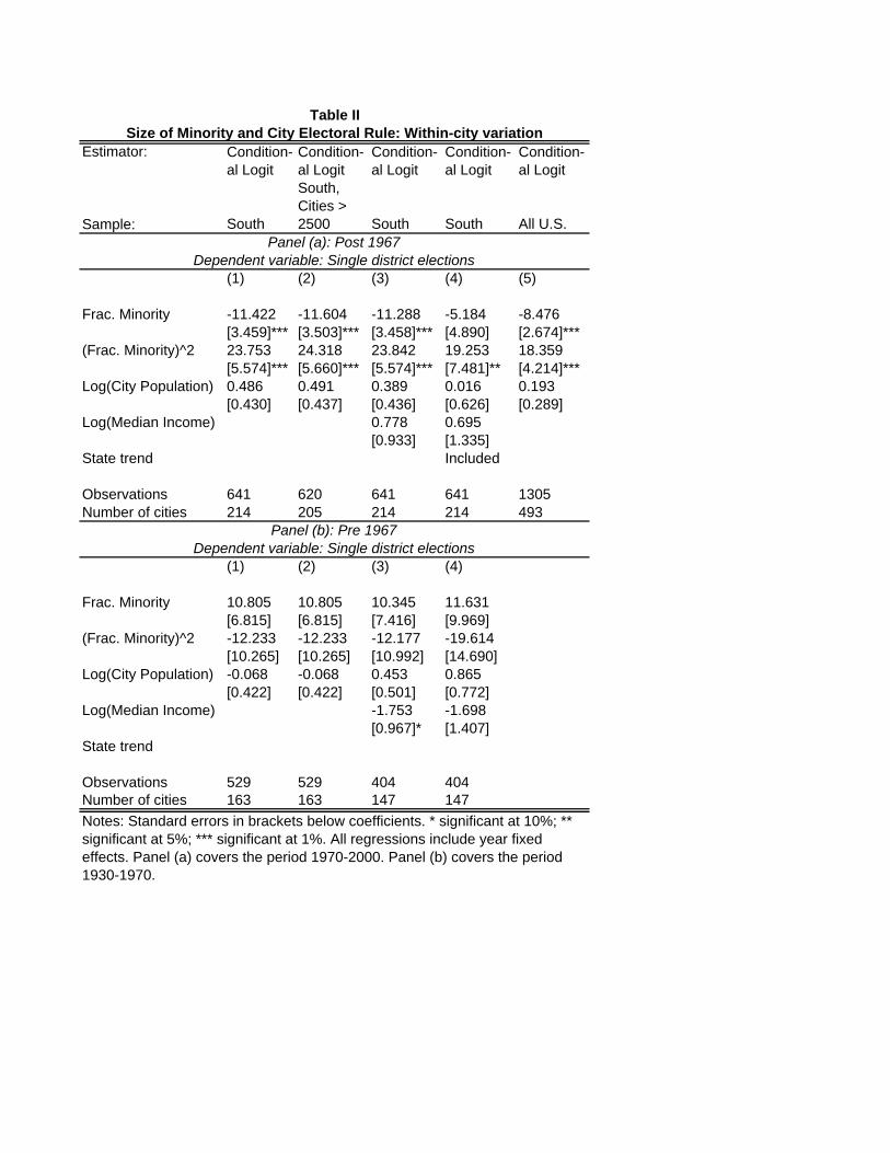
Table IISize of Minority and City Electoral Rule: Within-city variation

Estimator: Condition-al Logit

Condition-al Logit

Condition-al Logit

Condition-al Logit

Condition-al Logit

Sample: South

South, Cities > 2500 South South All U.S.

Panel (a): Post 1967Dependent variable: Single district elections

(1) (2) (3) (4) (5)

Frac. Minority -11.422 -11.604 -11.288 -5.184 -8.476[3.459]*** [3.503]*** [3.458]*** [4.890] [2.674]***

(Frac. Minority)^2 23.753 24.318 23.842 19.253 18.359[5.574]*** [5.660]*** [5.574]*** [7.481]** [4.214]***

Log(City Population) 0.486 0.491 0.389 0.016 0.193[0.430] [0.437] [0.436] [0.626] [0.289]

Log(Median Income) 0.778 0.695[0.933] [1.335]

State trend Included

Observations 641 620 641 641 1305Number of cities 214 205 214 214 493

Panel (b): Pre 1967Dependent variable: Single district elections

(1) (2) (3) (4)

Frac. Minority 10.805 10.805 10.345 11.631[6.815] [6.815] [7.416] [9.969]

(Frac. Minority)^2 -12.233 -12.233 -12.177 -19.614[10.265] [10.265] [10.992] [14.690]

Log(City Population) -0.068 -0.068 0.453 0.865[0.422] [0.422] [0.501] [0.772]

Log(Median Income) -1.753 -1.698[0.967]* [1.407]

State trend

Observations 529 529 404 404Number of cities 163 163 147 147Notes: Standard errors in brackets below coefficients. * significant at 10%; ** significant at 5%; *** significant at 1%. All regressions include year fixed effects. Panel (a) covers the period 1970-2000. Panel (b) covers the period 1930-1970.

Table IIISize of Minority and City Electoral Rule: Within-city variation

Estimator: Arellano-Bond GMM

Arellano-Bond GMM

Arellano-Bond GMM

Sample: South

South, Cities > 2500 All U.S.

Panel (a): Post 1967Dependent variable: Fraction of councilmen elected by district

(1) (2) (3)

Lag Single District 0.313 0.311 0.29[0.056]*** [0.055]*** [0.057]***

Frac. Minority -1.644 -1.654 -2.113[0.712]** [0.724]** [0.635]***

(Frac. Minority)^2 2.649 2.822 1.838[1.002]*** [0.972]*** [0.706]***

Log(City Population) -0.342 -0.33 -0.538[0.258] [0.275] [0.236]**

Second Order Serial Correlation p-value 0.140 0.140 0.196J test p-value 0.123 0.160 0.021Observations 1506 1489 2508Number of cities 797 782 1799

Panel (b): Pre 1967Dependent variable: Fraction of councilmen elected by district

(1) (2)

Lag Single District 0.751 0.751[0.109]*** [0.109]***

Frac. Minority 1.829 1.829[5.259] [5.259]

(Frac. Minority)^2 -3.634 -3.634[7.928] [7.928]

Log(City Population) 0.272 0.272[0.319] [0.319]

Second Order Serial Correlation p-value 0.07 0.07J test p-value 0.997 0.997Observations 891 891Number of cities 462 462Notes: Robust standard errors in brackets below coefficients. * significant at 10%; ** significant at 5%; *** significant at 1%. Lag Single District is the the first lag of the dependent variable. All regressions include year fixed effects. Panel (a) covers the period 1970-2000. Panel (b) covers the period 1930-1970. Both ethnic fractionalization and population are treated as endogenous variables. The maximum number of lags used for instrumenting them is 2.

Table IVChange in slope and t-stat of local

within regressions of single-district on fraction of minority (π) over the

range of π. Sample:South Slope t-stat

(1) (2)

post 1967 4.596 2.850[0.797]*** [0.473]***

South Slope t-stat(1) (2)

pre 1967 0.165 0.897[0.353] [0.926]

Notes: Column (1) reports coefficients and standard errors corresponding to regression of locally estimated coefficients of single-district on fraction of minority on the corresponding mid-sample fraction of minority. Column (2) employs the corresponding t-statistic. Robust standard errors are in brackets below coefficients. * significant at 10%; ** significant at 5%; *** significant at 1%. Regressions include a constant (not reported). See text for local sample details.

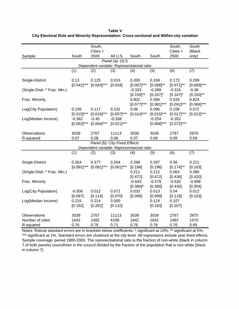
Table VCity Electoral Rule and Minority Representation: Cross-sectional and Within-city variation

Sample: South

South, Cities > 2500 All U.S. South South

South, Cities > 2500

South (Black only)

Panel (a): OLSDependent variable: Representaional ratio

(1) (2) (3) (4) (5) (6) (7)

Single-District 0.13 0.125 0.015 0.205 0.169 0.173 0.299[0.041]*** [0.043]*** [0.018] [0.067]*** [0.068]** [0.071]** [0.069]***

(Single-Distr. * Frac. Min.) -0.333 -0.289 -0.315 -0.38[0.159]** [0.157]* [0.167]* [0.163]**

Frac. Minority 0.802 0.586 0.533 0.824[0.077]*** [0.081]*** [0.091]*** [0.066]***

Log(City Population) 0.106 0.117 0.102 0.08 0.096 0.108 0.072[0.015]*** [0.016]*** [0.007]*** [0.014]*** [0.015]*** [0.017]*** [0.012]***

Log(Median Income) -0.362 -0.45 -0.338 -0.254 -0.352[0.062]*** [0.064]*** [0.021]*** [0.068]*** [0.072]***

Observations 3039 2767 11113 3039 3039 2767 2875R-squared 0.07 0.08 0.06 0.07 0.08 0.09 0.09

Panel (b): City Fixed EffectsDependent variable: Representaional ratio

(1) (2) (3) (4) (5) (6) (7)

Single-District 0.354 0.377 0.204 0.298 0.297 0.36 0.221[0.091]*** [0.081]*** [0.061]*** [0.196] [0.196] [0.174]** [0.163]

(Single-Distr. * Frac. Min.) 0.211 0.212 0.063 0.385[0.472] [0.472] [0.436] [0.420]

Frac. Minority -0.643 -0.579 -0.626 -0.568[0.380]* [0.380] [0.436] [0.354]

Log(City Population) -0.006 0.012 0.072 0.033 0.013 0.04 0.012[0.097] [0.114] [0.070] [0.096] [0.099] [0.118] [0.103]

Log(Median Income) 0.215 0.214 0.000 0.124 0.107[0.182] [0.202] [0.110] [0.183] [0.207]

Observations 3039 2767 11113 3039 3039 2767 2875Number of cities 1642 1482 6158 1642 1642 1482 1570R-squared 0.76 0.76 0.71 0.76 0.76 0.76 0.69Notes: Robust standard errors are in brackets below coefficients. * significant at 10%; ** significant at 5%; *** significant at 1%. Standard errors are clustered at the city level. All regressions include year fixed effects. Sample coverage: period 1980-2000. The representational ratio is the fraction of non-white (black in column 7 of both panels) councilmen in the council divided by the fraction of the population that is non-white (black in column 7).

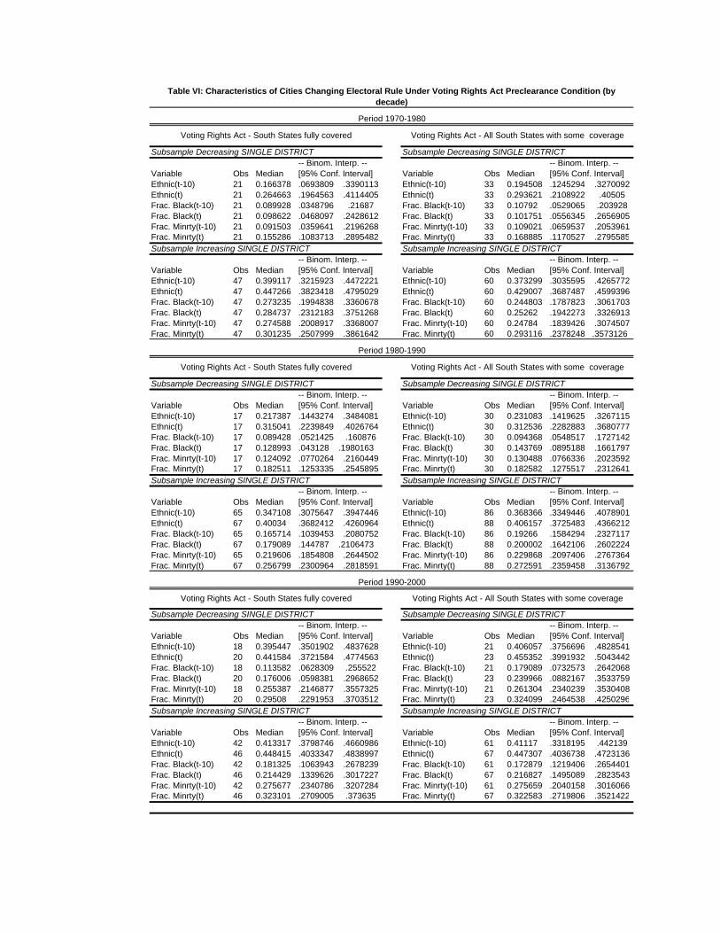
Table VI: Characteristics of Cities Changing Electoral Rule Under Voting Rights Act Preclearance Condition (by decade)

Period 1970-1980

Voting Rights Act - South States fully covered Voting Rights Act - All South States with some coverage

Subsample Decreasing SINGLE DISTRICT Subsample Decreasing SINGLE DISTRICT-- Binom. Interp. -- -- Binom. Interp. --

Variable Obs Median [95% Conf. Interval] Variable Obs Median [95% Conf. Interval]Ethnic(t-10) 21 0.166378 .0693809 .3390113 Ethnic(t-10) 33 0.194508 .1245294 .3270092Ethnic(t) 21 0.264663 .1964563 .4114405 Ethnic(t) 33 0.293621 .2108922 .40505Frac. Black(t-10) 21 0.089928 .0348796 .21687 Frac. Black(t-10) 33 0.10792 .0529065 .203928Frac. Black(t) 21 0.098622 .0468097 .2428612 Frac. Black(t) 33 0.101751 .0556345 .2656905Frac. Minrty(t-10) 21 0.091503 .0359641 .2196268 Frac. Minrty(t-10) 33 0.109021 .0659537 .2053961Frac. Minrty(t) 21 0.155286 .1083713 .2895482 Frac. Minrty(t) 33 0.168885 .1170527 .2795585Subsample Increasing SINGLE DISTRICT Subsample Increasing SINGLE DISTRICT

-- Binom. Interp. -- -- Binom. Interp. --Variable Obs Median [95% Conf. Interval] Variable Obs Median [95% Conf. Interval]Ethnic(t-10) 47 0.399117 .3215923 .4472221 Ethnic(t-10) 60 0.373299 .3035595 .4265772Ethnic(t) 47 0.447266 .3823418 .4795029 Ethnic(t) 60 0.429007 .3687487 .4599396Frac. Black(t-10) 47 0.273235 .1994838 .3360678 Frac. Black(t-10) 60 0.244803 .1787823 .3061703Frac. Black(t) 47 0.284737 .2312183 .3751268 Frac. Black(t) 60 0.25262 .1942273 .3326913Frac. Minrty(t-10) 47 0.274588 .2008917 .3368007 Frac. Minrty(t-10) 60 0.24784 .1839426 .3074507Frac. Minrty(t) 47 0.301235 .2507999 .3861642 Frac. Minrty(t) 60 0.293116 .2378248 .3573126

Period 1980-1990

Voting Rights Act - South States fully covered Voting Rights Act - All South States with some coverage

Subsample Decreasing SINGLE DISTRICT Subsample Decreasing SINGLE DISTRICT-- Binom. Interp. -- -- Binom. Interp. --

Variable Obs Median [95% Conf. Interval] Variable Obs Median [95% Conf. Interval]Ethnic(t-10) 17 0.217387 .1443274 .3484081 Ethnic(t-10) 30 0.231083 .1419625 .3267115Ethnic(t) 17 0.315041 .2239849 .4026764 Ethnic(t) 30 0.312536 .2282883 .3680777Frac. Black(t-10) 17 0.089428 .0521425 .160876 Frac. Black(t-10) 30 0.094368 .0548517 .1727142Frac. Black(t) 17 0.128993 .043128 .1980163 Frac. Black(t) 30 0.143769 .0895188 .1661797Frac. Minrty(t-10) 17 0.124092 .0770264 .2160449 Frac. Minrty(t-10) 30 0.130488 .0766336 .2023592Frac. Minrty(t) 17 0.182511 .1253335 .2545895 Frac. Minrty(t) 30 0.182582 .1275517 .2312641Subsample Increasing SINGLE DISTRICT Subsample Increasing SINGLE DISTRICT

-- Binom. Interp. -- -- Binom. Interp. --Variable Obs Median [95% Conf. Interval] Variable Obs Median [95% Conf. Interval]Ethnic(t-10) 65 0.347108 .3075647 .3947446 Ethnic(t-10) 86 0.368366 .3349446 .4078901Ethnic(t) 67 0.40034 .3682412 .4260964 Ethnic(t) 88 0.406157 .3725483 .4366212Frac. Black(t-10) 65 0.165714 .1039453 .2080752 Frac. Black(t-10) 86 0.19266 .1584294 .2327117Frac. Black(t) 67 0.179089 .144787 .2106473 Frac. Black(t) 88 0.200002 .1642106 .2602224Frac. Minrty(t-10) 65 0.219606 .1854808 .2644502 Frac. Minrty(t-10) 86 0.229868 .2097406 .2767364Frac. Minrty(t) 67 0.256799 .2300964 .2818591 Frac. Minrty(t) 88 0.272591 .2359458 .3136792

Period 1990-2000

Voting Rights Act - South States fully covered Voting Rights Act - All South States with some coverage

Subsample Decreasing SINGLE DISTRICT Subsample Decreasing SINGLE DISTRICT-- Binom. Interp. -- -- Binom. Interp. --

Variable Obs Median [95% Conf. Interval] Variable Obs Median [95% Conf. Interval]Ethnic(t-10) 18 0.395447 .3501902 .4837628 Ethnic(t-10) 21 0.406057 .3756696 .4828541Ethnic(t) 20 0.441584 .3721584 .4774563 Ethnic(t) 23 0.455352 .3991932 .5043442Frac. Black(t-10) 18 0.113582 .0628309 .255522 Frac. Black(t-10) 21 0.179089 .0732573 .2642068Frac. Black(t) 20 0.176006 .0598381 .2968652 Frac. Black(t) 23 0.239966 .0882167 .3533759Frac. Minrty(t-10) 18 0.255387 .2146877 .3557325 Frac. Minrty(t-10) 21 0.261304 .2340239 .3530408Frac. Minrty(t) 20 0.29508 .2291953 .3703512 Frac. Minrty(t) 23 0.324099 .2464538 .4250296Subsample Increasing SINGLE DISTRICT Subsample Increasing SINGLE DISTRICT

-- Binom. Interp. -- -- Binom. Interp. --Variable Obs Median [95% Conf. Interval] Variable Obs Median [95% Conf. Interval]Ethnic(t-10) 42 0.413317 .3798746 .4660986 Ethnic(t-10) 61 0.41117 .3318195 .442139Ethnic(t) 46 0.448415 .4033347 .4838997 Ethnic(t) 67 0.447307 .4036738 .4723136Frac. Black(t-10) 42 0.181325 .1063943 .2678239 Frac. Black(t-10) 61 0.172879 .1219406 .2654401Frac. Black(t) 46 0.214429 .1339626 .3017227 Frac. Black(t) 67 0.216827 .1495089 .2823543Frac. Minrty(t-10) 42 0.275677 .2340786 .3207284 Frac. Minrty(t-10) 61 0.275659 .2040158 .3016066Frac. Minrty(t) 46 0.323101 .2709005 .373635 Frac. Minrty(t) 67 0.322583 .2719806 .3521422

Notes: time period t for each variable refers to the final date of the period (for instance t=2000 for period 1990-2000). States fully covered under the 1975 renewal of the Voting Rights Act are Alabama, Georgia, Louisiana, Mississippi, South Carolina, Texas, and Virginia. Florida and North Carolina are only partially covered. Data exclude cities for which the change in electoral rule was dictated by court mandate or State law.

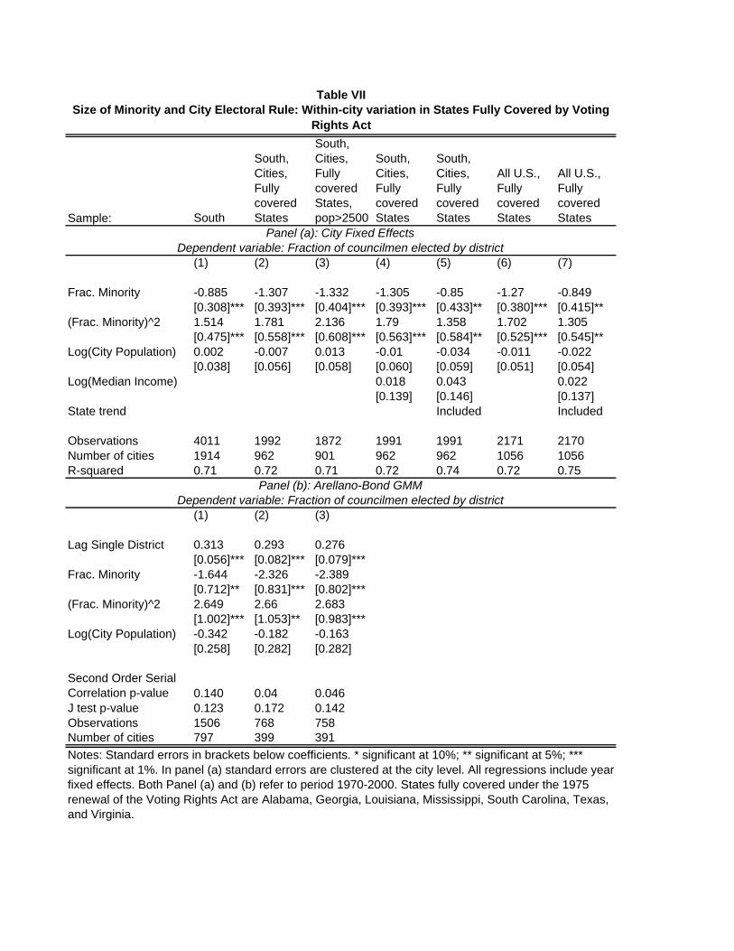
Table VIISize of Minority and City Electoral Rule: Within-city variation in States Fully Covered by Voting

Rights Act

Sample: South

South, Cities, Fully covered States

South, Cities, Fully covered States, pop>2500

South, Cities, Fully covered States

South, Cities, Fully covered States

All U.S., Fully covered States

All U.S., Fully covered States

Panel (a): City Fixed EffectsDependent variable: Fraction of councilmen elected by district

(1) (2) (3) (4) (5) (6) (7)

Frac. Minority -0.885 -1.307 -1.332 -1.305 -0.85 -1.27 -0.849[0.308]*** [0.393]*** [0.404]*** [0.393]*** [0.433]** [0.380]*** [0.415]**

(Frac. Minority)^2 1.514 1.781 2.136 1.79 1.358 1.702 1.305[0.475]*** [0.558]*** [0.608]*** [0.563]*** [0.584]** [0.525]*** [0.545]**

Log(City Population) 0.002 -0.007 0.013 -0.01 -0.034 -0.011 -0.022[0.038] [0.056] [0.058] [0.060] [0.059] [0.051] [0.054]

Log(Median Income) 0.018 0.043 0.022[0.139] [0.146] [0.137]

State trend Included Included

Observations 4011 1992 1872 1991 1991 2171 2170Number of cities 1914 962 901 962 962 1056 1056R-squared 0.71 0.72 0.71 0.72 0.74 0.72 0.75

Panel (b): Arellano-Bond GMMDependent variable: Fraction of councilmen elected by district

(1) (2) (3)

Lag Single District 0.313 0.293 0.276[0.056]*** [0.082]*** [0.079]***

Frac. Minority -1.644 -2.326 -2.389[0.712]** [0.831]*** [0.802]***

(Frac. Minority)^2 2.649 2.66 2.683[1.002]*** [1.053]** [0.983]***

Log(City Population) -0.342 -0.182 -0.163[0.258] [0.282] [0.282]

Second Order Serial Correlation p-value 0.140 0.04 0.046J test p-value 0.123 0.172 0.142Observations 1506 768 758Number of cities 797 399 391Notes: Standard errors in brackets below coefficients. * significant at 10%; ** significant at 5%; *** significant at 1%. In panel (a) standard errors are clustered at the city level. All regressions include year fixed effects. Both Panel (a) and (b) refer to period 1970-2000. States fully covered under the 1975 renewal of the Voting Rights Act are Alabama, Georgia, Louisiana, Mississippi, South Carolina, Texas, and Virginia.

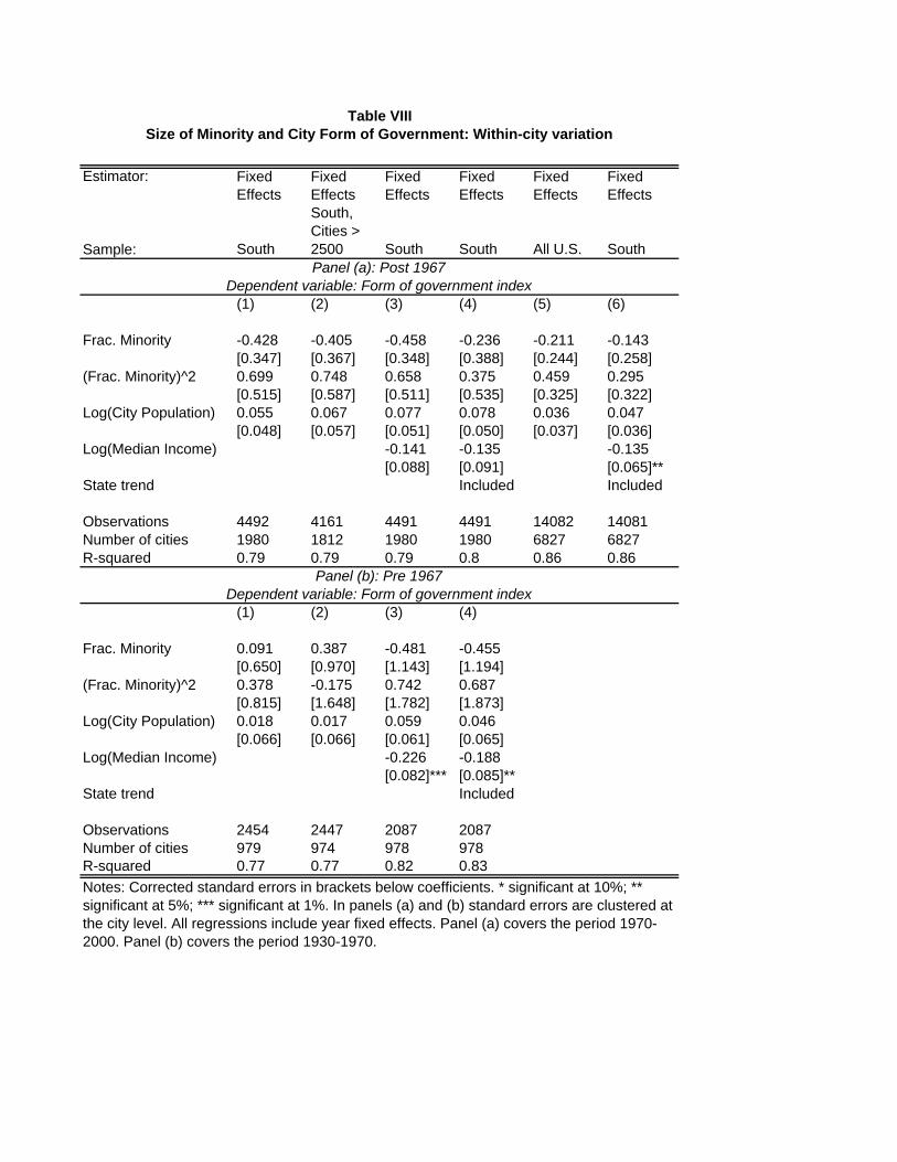
Table VIIISize of Minority and City Form of Government: Within-city variation

Estimator: Fixed Effects

Fixed Effects

Fixed Effects

Fixed Effects

Fixed Effects

Fixed Effects

Sample: South

South, Cities > 2500 South South All U.S. SouthPanel (a): Post 1967

Dependent variable: Form of government index(1) (2) (3) (4) (5) (6)

Frac. Minority -0.428 -0.405 -0.458 -0.236 -0.211 -0.143[0.347] [0.367] [0.348] [0.388] [0.244] [0.258]

(Frac. Minority)^2 0.699 0.748 0.658 0.375 0.459 0.295[0.515] [0.587] [0.511] [0.535] [0.325] [0.322]

Log(City Population) 0.055 0.067 0.077 0.078 0.036 0.047[0.048] [0.057] [0.051] [0.050] [0.037] [0.036]

Log(Median Income) -0.141 -0.135 -0.135[0.088] [0.091] [0.065]**

State trend Included Included

Observations 4492 4161 4491 4491 14082 14081Number of cities 1980 1812 1980 1980 6827 6827R-squared 0.79 0.79 0.79 0.8 0.86 0.86

Panel (b): Pre 1967Dependent variable: Form of government index

(1) (2) (3) (4)

Frac. Minority 0.091 0.387 -0.481 -0.455[0.650] [0.970] [1.143] [1.194]

(Frac. Minority)^2 0.378 -0.175 0.742 0.687[0.815] [1.648] [1.782] [1.873]

Log(City Population) 0.018 0.017 0.059 0.046[0.066] [0.066] [0.061] [0.065]

Log(Median Income) -0.226 -0.188[0.082]*** [0.085]**

State trend Included

Observations 2454 2447 2087 2087Number of cities 979 974 978 978R-squared 0.77 0.77 0.82 0.83Notes: Corrected standard errors in brackets below coefficients. * significant at 10%; ** significant at 5%; *** significant at 1%. In panels (a) and (b) standard errors are clustered at the city level. All regressions include year fixed effects. Panel (a) covers the period 1970-2000. Panel (b) covers the period 1930-1970.

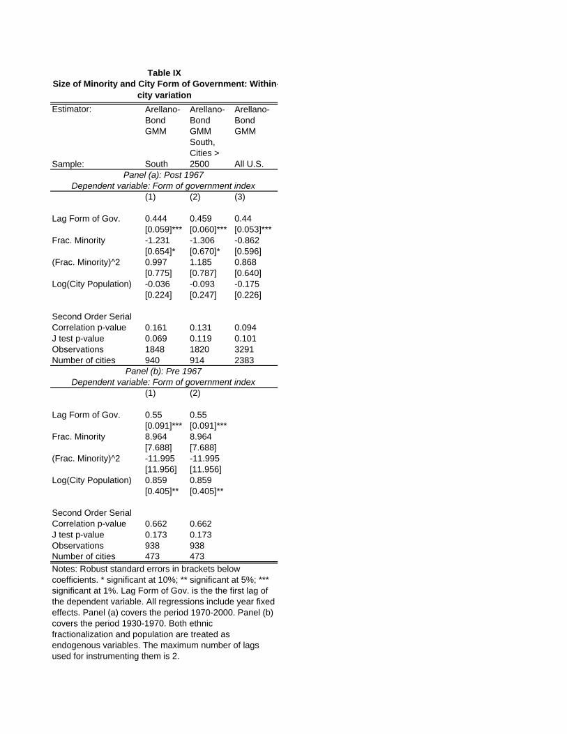
-Table IX

Size of Minority and City Form of Government: Withincity variation

Estimator: Arellano-Bond GMM

Arellano-Bond GMM

Arellano-Bond GMM

Sample: South

South, Cities > 2500 All U.S.

Panel (a): Post 1967Dependent variable: Form of government index

(1) (2) (3)

Lag Form of Gov. 0.444 0.459 0.44[0.059]*** [0.060]*** [0.053]***

Frac. Minority -1.231 -1.306 -0.862[0.654]* [0.670]* [0.596]

(Frac. Minority)^2 0.997 1.185 0.868[0.775] [0.787] [0.640]

Log(City Population) -0.036 -0.093 -0.175[0.224] [0.247] [0.226]

Second Order Serial Correlation p-value 0.161 0.131 0.094J test p-value 0.069 0.119 0.101Observations 1848 1820 3291Number of cities 940 914 2383

Panel (b): Pre 1967Dependent variable: Form of government index

(1) (2)

Lag Form of Gov. 0.55 0.55[0.091]*** [0.091]***

Frac. Minority 8.964 8.964[7.688] [7.688]

(Frac. Minority)^2 -11.995 -11.995[11.956] [11.956]

Log(City Population) 0.859 0.859[0.405]** [0.405]**

Second Order Serial Correlation p-value 0.662 0.662J test p-value 0.173 0.173Observations 938 938Number of cities 473 473Notes: Robust standard errors in brackets below coefficients. * significant at 10%; ** significant at 5%; *** significant at 1%. Lag Form of Gov. is the the first lag of the dependent variable. All regressions include year fixed effects. Panel (a) covers the period 1970-2000. Panel (b) covers the period 1930-1970. Both ethnic fractionalization and population are treated as endogenous variables. The maximum number of lags used for instrumenting them is 2.

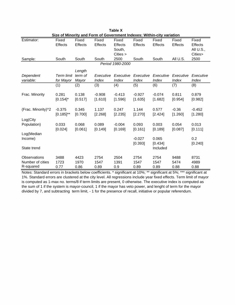
Table XSize of Minority and Form of Government Indexes: Within-city variation

Estimator: Fixed Effects

Fixed Effects

Fixed Effects

Fixed Effects

Fixed Effects

Fixed Effects

Fixed Effects

Fixed Effects

Sample: South South South

South, Cities > 2500 South South All U.S.

All U.S., Cities> 2500

Period 1980-2000

Dependent variable:

Term limit for Mayor

Length term of Mayor

Executive Index

Executive Index

Executive Index

Executive Index

Executive Index

Executive Index

(1) (2) (3) (4) (5) (6) (7) (8)

Frac. Minority 0.281 0.138 -0.908 -0.413 -0.927 -0.074 0.811 0.879[0.154]* [0.517] [1.610] [1.596] [1.635] [1.682] [0.954] [0.982]

(Frac. Minority)^2 -0.375 0.345 1.137 0.247 1.144 0.577 -0.36 -0.452[0.185]** [0.700] [2.268] [2.235] [2.270] [2.424] [1.260] [1.280]

Log(City Population) 0.033 0.068 0.089 -0.004 0.093 0.003 0.054 0.013

[0.024] [0.061] [0.149] [0.169] [0.161] [0.189] [0.087] [0.111]Log(Median Income) -0.027 0.065 0.2

[0.393] [0.434] [0.240]State trend Included

Observations 3488 4423 2754 2504 2754 2754 9488 8731Number of cities 1723 1970 1547 1391 1547 1547 5474 4989R-squared 0.77 0.86 0.89 0.9 0.89 0.89 0.88 0.88Notes: Standard errors in brackets below coefficients. * significant at 10%; ** significant at 5%; *** significant at 1%. Standard errors are clustered at the city level. All regressions include year fixed effects. Term limit of mayor is computed as 1-max no. terms/8 if term limits are present, 0 otherwise. The executive index is computed as the sum of 1 if the system is mayor-council, 1 if the mayor has veto power, and lenght of term for the mayor divided by 7, and subtracting term limit, - 1 for the presence of recall, initiative or popular referendum.

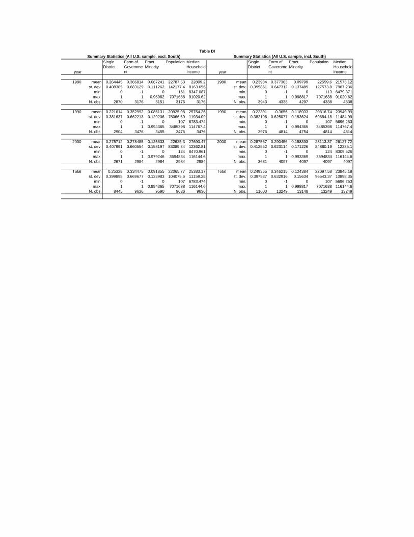
year

Single District

Form of Government

Fract. Minority

Population Median Household Income year

Single District

Form of Government

Fract. Minority

Population Median Household Income

1980 mean 0.264445 0.366814 0.067241 22787.53 22809.2 1980 mean 0.23934 0.377363 0.09799 22559.6 21573.12st. dev. 0.408385 0.683129 0.111262 142177.4 8163.656 st. dev. 0.395861 0.647312 0.137489 127573.8 7987.236

min. 0 -1 0 161 8347.087 min. 0 -1 0 113 6479.371max. 1 1 0.95962 7071638 91020.62 max. 1 1 0.998817 7071638 91020.62

N. obs. 2870 3176 3151 3176 3176 N. obs. 3943 4338 4297 4338 4338

1990 mean 0.221614 0.352992 0.085131 20925.98 25754.26 1990 mean 0.22391 0.3656 0.118933 20816.74 23949.99st. dev. 0.381637 0.662213 0.129206 75066.69 11934.09 st. dev. 0.382196 0.625077 0.153624 69684.18 11484.99

min. 0 -1 0 107 6783.474 min. 0 -1 0 107 5696.253max. 1 1 0.994365 3485398 114767.4 max. 1 1 0.994365 3485398 114767.4

N. obs. 2904 3476 3455 3476 3476 N. obs. 3976 4814 4754 4814 4814

2000 mean 0.275712 0.278485 0.125633 22625.3 27690.47 2000 mean 0.287567 0.290456 0.158393 23113.37 26127.72st. dev. 0.407991 0.660554 0.153197 83089.34 12362.81 st. dev. 0.412552 0.623114 0.171226 84880.19 12285.1

min. 0 -1 0 124 8470.961 min. 0 -1 0 124 8309.526max. 1 1 0.979246 3694834 116144.6 max. 1 1 0.993369 3694834 116144.6

N. obs. 2671 2984 2984 2984 2984 N. obs. 3681 4097 4097 4097 4097

Total mean 0.25328 0.334475 0.091855 22065.77 25383.17 Total mean 0.249355 0.346215 0.124384 22097.58 23845.18st. dev. 0.399898 0.669677 0.133983 104075.6 11159.28 st. dev. 0.397537 0.632916 0.15634 96543.37 10898.35

min. 0 -1 0 107 6783.474 min. 0 -1 0 107 5696.253max. 1 1 0.994365 7071638 116144.6 max. 1 1 0.998817 7071638 116144.6

N. obs. 8445 9636 9590 9636 9636 N. obs. 11600 13249 13148 13249 13249

Table DISummary Statistics (All U.S. sample, incl. South)Summary Statistics (All U.S. sample, excl. South)

year

Single District

Form of Government

Fract. Minority

Population

1930 mean 0.190187 0.614458 0.240152 55689.73st. dev. 0.341789 0.67566 0.152765 97710.1

min. 0 -1 0.00094 284.928max. 0.947368 1 0.96162 804874.1

N. obs. 144 166 137 137

1940 mean 0.367765 0.231325 0.221453 44127.13st. dev. 0.459492 0.795204 0.145513 85805.16

min. 0 -1 0.000239 4868max. 1 1 0.597693 859100.3

N. obs. 415 415 229 229

1950 mean 0.345231 0.254065 0.208854 32005.15st. dev. 0.452349 0.74599 0.144826 73305.76

min. 0 -1 0.000111 2774max. 1 1 0.723511 949708.4

N. obs. 486 492 492 492

1960 mean 0.253952 0.264264 0.194137 34242.28st. dev. 0.41375 0.675556 0.145493 82867.91

min. 0 -1 0 3202.001max. 1 1 0.694678 939023.6

N. obs. 656 666 663 663

1970 mean 0.161332 0.283726 0.17797 29274.97st. dev. 0.354326 0.555411 0.150278 79091.1

min. 0 -1 0 2406max. 1 1 0.770336 1199388

N. obs. 904 934 936 936

1980 mean 0.17219 0.406196 0.182536 21936.64st. dev. 0.351701 0.536582 0.164655 74266.77

min. 0 -1 0 113max. 1 1 0.998817 1595138

N. obs. 1073 1162 1146 1162

1990 mean 0.23013 0.398356 0.208838 20532.95st. dev. 0.383814 0.515051 0.175684 53238.92

min. 0 -1 0 243max. 1 1 0.986468 935926.6

N. obs. 1072 1338 1299 1338

2000 mean 0.318919 0.322552 0.246224 24421.92st. dev. 0.422985 0.50821 0.185563 89530.48

min. 0 -1 0 138max. 1 1 0.993369 1954847

N. obs. 1010 1113 1113 1113

Total mean 0.24545 0.33853 0.205515 26973.67st. dev. 0.401669 0.593737 0.166296 76418.88

min. 0 -1 0 113max. 1 1 0.998817 1954847

N. obs. 5760 6286 6015 6070

Table DIISummary Statistics (South sample)

South Region

Table DIII Voting Rights Act Coverage: Applicable Date; Fed. Register; Date

States Covered as a Whole: Alabama Nov. 1, 1964 30 FR 9897 Aug. 7, 1965. Alaska Nov. 1, 1972 40 FR 49422 Oct. 22, 1975. Arizona Nov. 1, 1972 40 FR 43746 Sept. 23, 1975. Georgia Nov. 1, 1964 30 FR 9897 Aug. 7, 1965. Louisiana Nov. 1, 1964 30 FR 9897 Aug. 7, 1965. Mississippi Nov. 1, 1964 30 FR 9897 Aug. 7, 1965. South Carolina Nov. 1, 1964 30 FR 9897 Aug. 7, 1965. Texas Nov. 1, 1972 40 FR 43746 Sept. 23, 1975. Virginia Nov. 1, 1964 30 FR 9897 Aug. 7, 1965. Covered Counties in States Not Covered as a Whole: California: Kings County Nov. 1, 1972 40 FR 43746 Sept. 23. 1975. Merced County Nov. 1, 1972 40 FR 43746 Sept. 23, 1975. Monterey County Nov. 1, 1968 36 FR 5809 Mar. 27, 1971. Yuba County Nov. 1, 1968 36 FR 5809 Mar. 27, 1971. Yuba County Nov. 1, 1972 41 FR 784 Jan. 5, 1976. Florida: Collier County Nov. 1, 1972 41 FR 34329 Aug. 13, 1976. Hardee County Nov. 1, 1972 40 FR 43746 Sept. 23, 1975. Hendry County Nov. 1, 1972 41 FR 34329 Aug. 13, 1976. Hillsborough County Nov. 1, 1972 40 FR 43746 Sept. 23, 1975. Monroe County Nov. 1, 1972 40 FR 43746 Sept. 23, 1975. New York: Bronx County Nov. 1, 1968 36 FR 5809 Mar. 27, 1971. Bronx County Nov. 1, 1972 40 FR 43746 Sept. 23, 1975. Kings County Nov. 1, 1968 36 FR 5809 Mar. 27, 1971. Kings County Nov. 1, 1972 40 FR 43746 Sept. 23, 1975. New York County Nov. 1, 1968 36 FR 5809 Mar. 27, 1971. North Carolina: Anson County Nov. 1, 1964 30 FR 9897 Aug. 7, 1965. Beaufort County Nov. 1, 1964 31 FR 5081 Mar. 29, 1966. Bertie County Nov. 1, 1964 30 FR 9897 Aug. 7, 1965. Bladen County Nov. 1, 1964 31 FR 5081 Mar. 29, 1966. Camden County Nov. 1, 1964 31 FR 3317 Mar. 2, 1966. Caswell County Nov. 1, 1964 30 FR 9897 Aug. 7, 1965. Chowan County Nov. 1, 1964 30 FR 9897 Aug. 7, 1965. Cleveland County Nov. 1, 1964 31 FR 5081 Mar. 29, 1966. Craven County Nov. 1, 1964 30 FR 9897 Aug. 7, 1965. Cumberland County Nov. 1, 1964 30 FR 9897 Aug. 7, 1965.

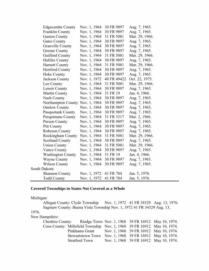
Edgecombe County Nov. 1, 1964 30 FR 9897 Aug. 7, 1965. Franklin County Nov. 1, 1964 30 FR 9897 Aug. 7, 1965. Gaston County Nov. 1, 1964 31 FR 5081 Mar. 29, 1966. Gates County Nov. 1, 1964 30 FR 9897 Aug. 7, 1965. Granville County Nov. 1, 1964 30 FR 9897 Aug. 7, 1965. Greene County Nov. 1, 1964 30 FR 9897 Aug. 7, 1965. Guilford County Nov. 1, 1964 31 FR 5081 Mar. 29, 1966. Halifax County Nov. 1, 1964 30 FR 9897 Aug. 7, 1965. Harnett County Nov. 1, 1964 31 FR 5081 Mar. 29, 1966. Hertford County Nov. 1, 1964 30 FR 9897 Aug. 7, 1965. Hoke County Nov. 1, 1964 30 FR 9897 Aug. 7, 1965. Jackson County Nov. 1, 1972 40 FR 49422 Oct. 22, 1975. Lee County Nov. 1, 1964 31 FR 5081 Mar. 29, 1966. Lenoir County Nov. 1, 1964 30 FR 9897 Aug. 7, 1965. Martin County Nov. 1, 1964 31 FR 19 Jan. 4, 1966. Nash County Nov. 1, 1964 30 FR 9897 Aug. 7, 1965. Northampton County Nov. 1, 1964 30 FR 9897 Aug. 7, 1965. Onslow County Nov. 1, 1964 30 FR 9897 Aug. 7, 1965. Pasquotank County Nov. 1, 1964 30 FR 9897 Aug. 7, 1965. Perquimans County Nov. 1, 1964 31 FR 3317 Mar. 2, 1966. Person County Nov. 1, 1964 30 FR 9897 Aug. 7, 1965. Pitt County Nov. 1, 1964 30 FR 9897 Aug. 7, 1965. Robeson County Nov. 1, 1964 30 FR 9897 Aug. 7, 1965. Rockingham County Nov. 1, 1964 31 FR 5081 Mar. 29, 1966. Scotland County Nov. 1, 1964 30 FR 9897 Aug. 7, 1965. Union County Nov. 1, 1964 31 FR 5081 Mar. 29, 1966. Vance County Nov. 1, 1964 30 FR 9897 Aug. 7, 1965. Washington County Nov. 1, 1964 31 FR 19 Jan. 4, 1966. Wayne County Nov. 1, 1964 30 FR 9897 Aug. 7, 1965. Wilson County Nov. 1, 1964 30 FR 9897 Aug. 7, 1965. South Dakota: Shannon County Nov. 1, 1972 41 FR 784 Jan. 5, 1976. Todd County Nov. 1, 1972 41 FR 784 Jan. 5, 1976. Covered Townships in States Not Covered as a Whole Michigan: Allegan County: Clyde Township Nov. 1, 1972 41 FR 34329 Aug. 13, 1976. Saginaw County: Buena Vista Township Nov. 1, 1972 41 FR 34329 Aug. 13, 1976. New Hampshire: Cheshire County: Rindge Town Nov. 1, 1968 39 FR 16912 May 10, 1974. Coos County: Millsfield Township Nov. 1, 1968 39 FR 16912 May 10, 1974. Pinkhams Grant Nov. 1, 1968 39 FR 16912 May 10, 1974. Stewartstown Town Nov. 1, 1968 39 FR 16912 May 10, 1974. Stratford Town Nov. 1, 1968 39 FR 16912 May 10, 1974.

Grafton County: Benton Town Nov. 1, 1968 39 FR 16912 May 10, 1974. Hillsborough County: Antrim Town Nov. 1, 1968 39 FR 16912 May 10, 1974. Merrimack County: Boscawen Town Nov. 1, 1968 39 FR 16912 May 10, 1974. Rockingham County: Newington Town Nov. 1, 1968 39 FR 16912 May 10, 1974. Sullivan County: Unity Town Nov. 1, 1968 39 FR 16912 May 10, 1974. Source: Department of Justice.

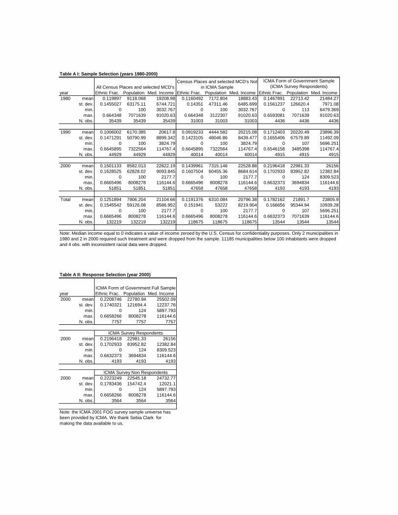
year Ethnic Frac. Population Med. Income Ethnic Frac. Population Med. Income Ethnic Frac. Population Med. Income1980 mean 0.119897 9118.068 19208.98 0.1160492 7172.804 18883.43 0.1467891 22713.42 21484.27

st. dev. 0.1455027 63175.11 6744.721 0.14351 47311.46 6485.699 0.1561237 126620.4 7971.08min. 0 100 3032.767 0 100 3032.767 0 113 6479.369

max. 0.664348 7071639 91020.63 0.664348 3122307 91020.63 0.6593081 7071639 91020.63N. obs. 35439 35439 35439 31003 31003 31003 4436 4436 4436

1990 mean 0.1006002 6170.385 20617.8 0.0919233 4444.582 20215.08 0.1712403 20220.49 23896.39st. dev. 0.1471291 50790.99 8899.342 0.1423105 48046.86 8439.477 0.1655406 67579.89 11492.09

min. 0 100 3824.79 0 100 3824.79 0 107 5696.251max. 0.6645895 7322564 114767.4 0.6645895 7322564 114767.4 0.6546158 3485398 114767.4

N. obs. 44929 44929 44929 40014 40014 40014 4915 4915 4915

2000 mean 0.1501133 8582.013 22822.19 0.1439961 7315.146 22528.88 0.2196418 22981.33 26156st. dev. 0.1628525 62828.02 9093.845 0.1607504 60455.36 8684.614 0.1702933 83952.82 12382.84

min. 0 100 2177.7 0 100 2177.7 0 124 8309.523max. 0.6665496 8008278 116144.6 0.6665496 8008278 116144.6 0.6632373 3694834 116144.6

N. obs. 51851 51851 51851 47658 47658 47658 4193 4193 4193

Total mean 0.1251894 7906.204 21104.66 0.1191376 6310.084 20796.38 0.1782162 21891.7 23805.9st. dev. 0.1545542 59126.08 8586.952 0.151941 53222 8219.904 0.166656 95344.94 10939.28

min. 0 100 2177.7 0 100 2177.7 0 107 5696.251max. 0.6665496 8008278 116144.6 0.6665496 8008278 116144.6 0.6632373 7071639 116144.6

N. obs. 132219 132219 132219 118675 118675 118675 13544 13544 13544

Note: Median income equal to 0 indicates a value of income zeroed by the U.S. Census for confidentiality purposes. Only 2 municipalities in 1980 and 2 in 2000 required such treatment and were dropped from the sample. 11185 municipalities below 100 inhabitants were dropped and 4 obs. with inconsistent racial data were dropped.

Table A I: Sample Selection (years 1980-2000)Census Places and selected MCD's Not

in ICMA SampleICMA Form of Government Sample

(ICMA Survey Respondents)All Census Places and selected MCD's

year Ethnic Frac. Population Med. Income2000 mean 0.2208746 22780.94 25502.09

st. dev. 0.1740321 121694.4 12237.76min. 0 124 5897.793

max. 0.6658266 8008278 116144.6N. obs. 7757 7757 7757

2000 mean 0.2196418 22981.33 26156st. dev. 0.1702933 83952.82 12382.84

min. 0 124 8309.523max. 0.6632373 3694834 116144.6

N. obs. 4193 4193 4193

2000 mean 0.2223249 22545.18 24732.77st. dev. 0.1783436 154742.4 12021.1

min. 0 124 5897.793max. 0.6658266 8008278 116144.6

N. obs. 3564 3564 3564

Note: the ICMA 2001 FOG survey sample universe has been provided by ICMA. We thank Sebia Clark for making the data available to us.

Table A II: Response Selection (year 2000)

ICMA Form of Government Full Sample

ICMA Survey Respondents

ICMA Survey Non Respondents

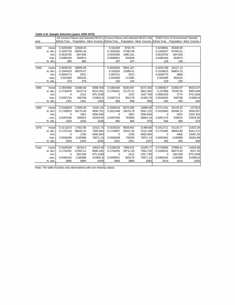
year Ethnic Frac. Population Med. Income Ethnic Frac. Population Med. Income Ethnic Frac. Population Med. Income

1930 mean 0.3292589 22008.04 . 0.331009 8764.79 . 0.3248581 55308.09 .st. dev. 0.1502718 60550.19 . 0.1526281 27382.69 . 0.1446257 97456.01 .

min. 0.0018783 284.928 . 0.0042565 1985.251 . 0.0018783 284.928 .max. 0.6480194 804874 . 0.5599921 505508 . 0.6480194 804874 .

N. obs. 485 485 . 347 347 . 138 138 .

1940 mean 0.3030753 28999.28 . 0.3029203 5904.107 . 0.3031768 44127.13 .st. dev. 0.1564919 69525.07 . 0.162654 10389.01 . 0.1526823 85805.15 .

min. 0.0004773 2522 . 0.003721 2522 . 0.0004773 4868 .max. 0.501893 859100 . 0.501893 111580 . 0.500385 859100 .

N. obs. 379 379 . 150 150 . 229 229 .

1950 mean 0.2554969 15490.66 9398.706 0.2360436 6030.967 9272.253 0.2893527 31953.97 9619.227st. dev. 0.1734978 52227.8 6513.281 0.1790261 31175.21 3651.893 0.157986 73240.03 9654.049

min. 0 1012 975.1038 0 1012 1937.759 0.0002228 2774 975.1038max. 0.5287216 949708 215854.8 0.5287216 802178 41493.78 0.5028492 949708 215854.8

N. obs. 1351 1351 1350 858 858 858 493 493 492

1960 mean 0.2346919 17858.46 13421.45 0.2094234 6570.596 13895.89 0.2711151 34129.25 12728.9st. dev. 0.1769923 58170.46 4990.751 0.1821448 26076.79 5552.122 0.1626483 82698.15 3936.007

min. 0 1851 2094.594 0 1851 2094.594 0 3202 2324.324max. 0.5097046 939024 42929.05 0.5097046 763956 36564.19 0.5051175 939024 42929.05

N. obs. 1626 1626 1648 960 960 978 666 666 670

1970 mean 0.2113373 17452.66 21521.73 0.2018225 9929.842 21489.66 0.2412711 41119.77 21622.34st. dev. 0.1742144 58033.25 7005.694 0.1744557 32521.35 7413.138 0.1701882 99564.85 5541.271

min. 0 1235 4692.664 0 1235 4692.664 0 4906 10051.55max. 0.5558298 1199388 76871.13 0.5558298 730359 76871.13 0.5053402 1199388 59262.89

N. obs. 2044 2044 2040 1551 1551 1547 493 493 493

Total mean 0.2435539 18233.4 15623.49 0.2268228 7969.613 16195.77 0.2755909 37886.61 14453.68st. dev. 0.1754291 57900.31 8089.185 0.1794255 29711.03 7994.725 0.1628231 86579.32 8157.32

min. 0 284.928 975.1038 0 1012 1937.759 0 284.928 975.1038max. 0.6480194 1199388 215854.8 0.5599921 802178 76871.13 0.6480194 1199388 215854.8

N. obs. 5885 5885 5038 3866 3866 3383 2019 2019 1655

Note: The table includes only observations with non missing values.

Table A III: Sample Selection (years 1930-1970)All Census Places and selected MCD's Census Places and selected MCD's Not ICMA Form of Government Sample