nber working paper series energy productivity and energy
TRANSCRIPT

NBER WORKING PAPER SERIES
ENERGY PRODUCTIVITY AND ENERGY DEMAND:EXPERIMENTAL EVIDENCE FROM INDIAN MANUFACTURING PLANTS
Nicholas Ryan
Working Paper 24619http://www.nber.org/papers/w24619
NATIONAL BUREAU OF ECONOMIC RESEARCH1050 Massachusetts Avenue
Cambridge, MA 02138May 2018
I thank Esther Duflo, Michael Greenstone and Rohini Pande for guidance and Nicholas Bloom for early encouragement. R N Pandya of the Gujarat Energy Development Agency gave implementation support. Harsh Singh, Harsh Vijay Singh, Vipin Awatramani, Raunak Kalra and Maulik Chauhan provided exemplary research assistance. Seminar audiences at Boston University, Brown, Carnegie Mellon, Chicago, Cornell, LSE, Michigan, Michigan State, Namurs, NBER EEE, NEUDC, PSE, Stanford, Toulouse and Virginia provided useful feedback. I thank Namrata Kala and Joe Shapiro for detailed comments. The MIT Energy Initiative, Veolia Environment, US AID – Development Innovation Ventures (Award number AID-OAA- G-12-00007), the Sustainability Science Program at Harvard and Private Enterprise Development in Low-income Countries (PEDL) (Exploratory Grant number 1657) provided financial support. All views and errors are my own. The views expressed herein are those of the author and do not necessarily reflect the views of the National Bureau of Economic Research.
NBER working papers are circulated for discussion and comment purposes. They have not been peer-reviewed or been subject to the review by the NBER Board of Directors that accompanies official NBER publications.
© 2018 by Nicholas Ryan. All rights reserved. Short sections of text, not to exceed two paragraphs, may be quoted without explicit permission provided that full credit, including © notice, is given to the source.

Energy Productivity and Energy Demand: Experimental Evidence from Indian ManufacturingPlantsNicholas RyanNBER Working Paper No. 24619May 2018JEL No. D24,O14,Q41
ABSTRACT
This paper studies a field experiment among energy-intensive Indian manufacturing plants that offered energy consulting to raise energy productivity, the amount plants can produce with each unit of energy. Treatment plants, after two years and relative to the control, run longer hours, demand more skilled labor and use 9.5 percent more electricity (standard error 7.3 percent). I assume that the treatment acted only through energy productivity to estimate the plant production function. The model estimates imply that energy complements skill and capital and that energy demand therefore responds more strongly to a productivity shock when plants can adjust these inputs.
Nicholas RyanDepartment of EconomicsYale UniversityP. O. Box 208269New Haven, CT 06520and [email protected]

Energy Productivity and Energy Demand:
Experimental Evidence from Indian Manufacturing Plants∗
Nicholas Ryan†
May 7, 2018
Abstract
This paper studies a field experiment among energy-intensive Indian manufacturingplants that offered energy consulting to raise energy productivity, the amount plantscan produce with each unit of energy. Treatment plants, after two years and relativeto the control, run longer hours, demand more skilled labor and use 9.5 percent moreelectricity (standard error 7.3 percent). I assume that the treatment acted only throughenergy productivity to estimate the plant production function. The model estimatesimply that energy complements skill and capital and that energy demand thereforeresponds more strongly to a productivity shock when plants can adjust these inputs.JEL Codes: O14, Q41, D24, L65, L67
I Introduction
In the last two decades, coal consumption in India has tripled and in China quadrupled,
while declining slightly in most industrialized countries (Energy Information Administra-
tion, 2016). In the decades to come, growth in energy consumption is forecast to be four
times higher outside the OECD than within. Any plan to address global climate change
must therefore reduce or de-carbonize energy consumption in developing countries.
The direction of global policy has been to move towards this goal without setting binding
emissions targets or prices for poorer countries. Recent climate agreements have focused on
pushing climate goods as much as taxing bads. For example, the Copenhagen Accords and
∗I thank Esther Duflo, Michael Greenstone and Rohini Pande for guidance and Nicholas Bloom for earlyencouragement. R N Pandya of the Gujarat Energy Development Agency gave implementation support.Harsh Singh, Harsh Vijay Singh, Vipin Awatramani, Raunak Kalra and Maulik Chauhan provided exemplaryresearch assistance. Seminar audiences at Boston University, Brown, Carnegie Mellon, Chicago, Cornell,LSE, Michigan, Michigan State, Namurs, NBER EEE, NEUDC, PSE, Stanford, Toulouse and Virginiaprovided useful feedback. I thank Namrata Kala and Joe Shapiro for detailed comments. The MIT EnergyInitiative, Veolia Environment, US AID – Development Innovation Ventures (Award number AID-OAA-G-12-00007), the Sustainability Science Program at Harvard and Private Enterprise Development in Low-income Countries (PEDL) (Exploratory Grant number 1657) provided financial support. All views anderrors are my own.†Yale University, Dept. of Economics, Box 208269, New Haven, CT 06520-8269, [email protected]
1

Paris Agreement stated a goal of USD 100 billion per year in climate finance to flow from
developed to developing countries by 2020, for greenhouse gas mitigation and climate adap-
tation (ClimateFocus, 2016).1 In the same spirit of checking emissions without retarding
growth, China and India have set targets for carbon intensity per unit output, rather than
directly for emissions (Stern and Jotzo, 2010). Not only are these aggregate targets set in
intensity terms, but many specific policy actions are directed towards subsidizing efficiency
rather than reducing energy use per se. A recent head of the UN Climate Change Secre-
tariat proclaimed “Energy efficiency is the most promising means to reduce greenhouse gas
emission in the short term” (Doyle, 2007).
This drive for efficiency may be misguided to the extent efficiency does not lower energy
use or carbon emissions. Figure 1 plots the relationship between energy-efficiency and
output in two contexts. Panel A shows the cross-country relationship between energy use
and energy productivity (output per unit energy), using data from the World Bank. Panel
B shows, in the control group of the sample of energy-intensive plants studied in this
paper, the relationship between electricity use and an index of efficiency based on physical
measurements within plants. In both cases, energy use is strongly increasing with respect
to energy efficiency.2 A long-standing line of thought in energy economics suggests that
efficiency may cause higher energy consumption, by lowering the effective price of energy
services (Jevons, 1905). In this view, in the long run, all increases in the productivity of
energy may be offset, or more than offset, by an ever-expanding demand for energy services
(Nordhaus, 1996).
This paper studies the causal effect of energy productivity on energy use using a field
experiment that offered energy consulting to Indian manufacturing plants. The experiment
recruited a sample of over four hundred manufacturing plants from the textile and chemical
sectors. These plants are large, with a mean employment at baseline of 83 people, and
energy-intensive, with roughly USD 200 thousand in annual energy costs and monthly
electricity use equal to that of 66 American homes. The main experimental intervention
is an industrial energy audit, sponsored in part by the Department of Climate Change,
Government of Gujarat, the first state-level climate change department in India. Since
1This goal is underfunded and there has been a fierce debate, since its inception, about the extent ofunderfunding and whether commitments are additional to existing aid and capital flows (Organization forEconomic Cooperation and Development, 2015; Climate Change Finance Unit, 2015).
2The coefficient for a regression of log energy use on efficiency is 0.33 log points (standard error 0.10) perstandard deviation of efficiency across countries and 1.67 log points (standard error 0.21) across plants.
2

skilled labor may be complementary to energy productivity, a second treatment arm offered
half of audited plants a part-time engineer to implement audit recommendations.
To evaluate the plant response to energy consulting, I collect data on plant inputs,
investment and outputs in an endline survey completed on average 27 months after the
intervention. The endline survey recorded plant input demands in a manner similar to the
Annual Survey of Industries, which has been used to study energy shocks in India (Allcott,
Collard-Wexler and O’Connell, 2014). The plant survey also includes within-plant physical
measurements to record changes in efficiency and operating practices. I supplement this
survey data collection with administrative records from power utilities on the electricity
consumption of sample plants over a period of three years, starting six months prior to the
intervention.
The reduced-form results of the experiment show that the treatment did not reduce
energy use as projected and suggest that treatment plants respond to increases in energy
productivity by using more energy. Energy audits were projected to reduce plant energy
consumption by ten percent. The point estimate for the effect of treatment on electricity
demand, by contrast, is positive and grows to 9.5 percent (standard error 7.3 percent) after
two years. The experiment can therefore reject that energy use declined as predicted (p-
value < 0.01) but not that there was no change in energy use (p-value = 0.17). Physical
measurements within the plant were used to calculate an efficiency index representative of
all energy-using equipment. I find that in treatment plants this index is on average 0.085
standard deviations (standard error 0.065 standard deviations) higher for all systems, and
shows a large increase for the boiler, the single most important energy-using system in the
plant. The plant survey also finds that plant-floor staff in treatment plants report running
equipment 1.12 hours per day (standard error 0.49 hours) longer than in control plants, an
increase in capacity utilization of seven percent.
Increases in energy use may change other factor demands depending on the comple-
mentarity or substitutability of energy with other inputs. Energy may substitute for labor;
I observed sample plants in which men fed coal into a steam boiler and others in which
machines (an electric coal crusher and conveyor belt) did the same task. Energy may also
complement labor, in that using energy requires monitoring and maintaining a wide range
of plant equipment, for example by checking the temperature of a chemical reaction or
tightening the belt that connects a motor to a textile printing machine.
3

I find that treatment plants modernize their input mix in response to energy consulting.
At endline, I estimate a large and highly statistically significant increase in skilled labor
demand in the treatment relative to the control plants. The increase in skill demand is seen
both for managers and for technical and supervisory workers on the shop floor. Demand
for unskilled labor is constant in the treatment, despite the increase in plant capacity
utilization. The point estimate for plant capital at endline is positive and large, though
imprecisely estimated and only statistically significant at the ten percent level.
The pattern of experimental results suggests a plant production function where energy
is complementary to skilled labor and capital but may be substituted for unskilled labor. I
specify a nested constant elasticity of substitution production function consistent with these
patterns of input substitution. In the production model, the treatment is represented by a
change in the factor-specific productivity of energy from ∆ = 1 to some unknown ∆ = ∆1,
meaning that treatment plants may produce more energy services for the same number
of kilowatt-hours or British thermal units used. I construct an estimator to match the
input demands for energy, capital, skilled labor, unskilled labor and materials in the control
and treatment groups to those predicted by the model. The key identifying assumption is
that the changes in input demands observed in the treatment are due only to increases in
energy productivity. This exogenous single-factor productivity shock allows me to identify
the production function without using the cross-sectional correlations of input demands
across plants, which would confound substitution parameters with unobserved shocks to
total factor productivity.
Estimates of the production function model are consistent with the reduced-form results
cited above and allow us to quantify changes in energy productivity at the plant level. I
estimate energy productivity increased by six percent in the textile sector plants and ten
percent in chemical sector plants. In order to fit the modernization of plants’ input mix, the
estimated production function parameters show that energy is substitutable for the basic
inputs of materials and unskilled labor, while the basic input nest (of energy, materials and
unskilled labor together) is highly complementary with skilled labor and capital.
The production function estimates allow analysis of the change in social surplus due
to an energy productivity shock. Higher productivity has ambiguous effects on surplus
because it increases profits but, depending on production parameters, may also increase
the external costs of energy use. I consider counterfactuals on two dimensions, first, the
4

flexibility of plant inputs in response to energy productivity and second, whether energy
productivity is subsidized or an energy tax is applied instead. Energy use will respond
to energy productivity differently depending on the flexibility of inputs. Energy audit
projections take all other plant inputs as given, following engineering practice. I use the
model to estimate this direct effect of energy productivity on energy use and then to predict
the effect when only energy input can change (the short-term effect) and the effect when
all factors of production can adjust (the medium-term effect).
I find that energy use, in the model, declines directly and in the short-term but increases
sharply in the medium-term once all input factors can adjust. The reason for this swing,
given the production function estimates, is straightforward: energy is highly complemen-
tary to capital and skilled labor and so a plant’s desired increase in energy demand is much
greater if it can change these factor inputs at the same time. Though energy use increases
sharply at longer horizons, plant profits are steady, near the direct effect of energy pro-
ductivity on profits, an instance of the envelope theorem for small changes in single-factor
productivity. These findings on factor adjustment are consistent with macroeconomic mod-
els of how energy use responds to price shocks at different time horizons (Pindyck and
Rotemberg, 1983; Atkeson and Kehoe, 1999).
In the second set of counterfactuals I compare the social surplus under energy policy
regimes that either endow plants with higher energy productivity (as through subsidies for
energy consulting or equipment) or instead impose a Pigouvian tax on energy use. I calibrate
the level of the tax to match the decline in energy use due to the direct effect of energy
productivity estimated for the experiment. I measure social surplus as the sum of profits and
the social costs of energy use, using estimates from the literature of the external damages
of coal and natural gas consumption in India. Depending on the valuation of external costs,
the social surplus from sample plants’ production can be near zero or negative.3
The main finding from the counterfactuals is that feasible energy productivity policies,
which allow for factor adjustment, reduce surplus. A policy that was able to achieve only
the direct effect of raising energy productivity, at a constant level of energy service, would
necessarily raise surplus, since higher productivity increases plant profits through lower
3For textile plants, which spend more on energy at private cost than they earn in profits, I calculate valueadded net of external costs of energy use of negative USD 394 thousand per plant. Muller, Mendelsohn andNordhaus (2011) find negative social value added for a number of sectors in the US economy, includingcoal-based power generation.
5

energy bills and, at a constant level of energy service, must also reduce energy use. However,
in the feasible case, plant factor demands respond to higher energy productivity, which raises
energy use and therefore external costs. In the estimated model, endowing plants with
higher energy productivity reduces social surplus because the increase in energy demand
raises social costs more than productivity raises profits. The calibrated energy tax, by
contrast, modestly increases surplus with endogenous factor demands. Using the model, I
calculate a difference in social surplus under energy tax versus energy productivity policies
of USD 70 thousand per textile plant and USD 12 thousand per chemical plant.
The results contribute to the literatures on energy-efficiency and the productivity of
developing-country firms. On energy-efficiency, a recent burst of research has generally
found energy savings from efficiency upgrades well below ex ante projections.4 Davis, Fuchs
and Gertler (2014) find that subsidizing efficient appliances for households reduced electric-
ity consumption far less than expected in Mexico and that indeed households increased
electricity demand after getting more efficient air conditioners. There is relatively little
evidence on either energy-efficiency in developing countries or on the behavior of firms in
response to efficiency upgrades.5
On developing-country firm productivity, there is an active literature quantifying the
dispersion in productivity across manufacturing plants and over their life cycles (Hsieh and
Klenow, 2009, 2014). It is a relatively open question to what extent this dispersion in
productivity is due to market failures, onerous regulation or plant responses to different
economic environments.6 Several experiments try to test the constraints to firm productiv-
ity and growth by exogenously removing particular constraints (e.g. De Mel, McKenzie and
Woodruff, 2013, on formalization). Most prior studies focus on micro-enterprises. The clos-
4Allcott and Greenstone (2012) decry the paucity of evidence on energy efficiency circa 2012. Fowlie,Greenstone and Wolfram (2017) use a field experiment to find large negative returns to residential weatheriza-tion (insulation and related measures) in Michigan due to very low realized savings. Allcott and Greenstone(2017) use a field experiment to find negative returns to weatherization in Wisconsin due both to low real-ized returns and to experimental complier households having a low tendency to invest. Burlig et al. (2017)estimate the savings due to efficiency upgrades in California schools with a machine learning model appliedto highly detailed energy consumption data and find low realized savings.
5Anderson and Newell (2004) study the United States Department of Energy’s long-standing IndustrialAssessment Centers program, which provides industrial energy audits, but have data only on projectedsavings and measure take-up and not ex post energy use. Adhvaryu, Kala and Nyshadham (2018) usehigh-frequency production data to estimate that line-level productivity increases after factories install LEDlights, which use less energy and generate less heat, and find that this increase in productivity is greater athigher temperatures.
6Asker, Collard-Wexler and Loecker (2014) argue that productivity dispersion can be rationalized bycapital adjustment costs and differing volatilities of developed and developing economics. Hsieh and Olken(2014) find no evidence of regulatory distortions in the firm size distributions of several countries.
6

est precedents to this paper are Bruhn, Karlan and Schoar (2018) and Bloom et al. (2013),
which offer management consulting services to Mexican Small- and Medium-Enterprises
(averaging 14 employees) and Indian textile mills (270 employees), respectively. In com-
mon with Bruhn, Karlan and Schoar (2018), the present study sample includes hundreds
of plants and measures the effect of consulting on input demands. In common with Bloom
et al. (2013), this paper studies the productivity response to consulting among large Indian
plants. Because the consulting intervention in this study is energy-specific, this paper can
isolate the impact of a particular factor productivity shock on factor demands and produc-
tion, in a way that prior multi-pronged interventions could not.7 I apply this exclusion
restriction, that the treatment only acts through one input, to transparently estimate the
plant production function, a method that may be useful for the analysis of other field exper-
iments designed to shock input prices or productivity. Finally, the focus on measurement of
productivity and energy use is also highly relevant to climate policy, since the intervention
studied here is itself a climate policy, of a type widely supported by national and global
subsidies.
The rest of the paper runs as follows. Section II describes the setting for the study,
the design of the experiment and the interventions. Section III describes the reduced-form
results, with an emphasis on how the treatment changed plants’ input demands. Section IV
introduces a production function model to measure the effect of the treatment on plants’
energy productivity. Section V estimates the model and evaluates in counterfactuals how
profits and social surplus respond to energy productivity as compared to energy taxes.
Section VI concludes.
II Context and Experimental Design
II.A Energy-efficiency policy in India
Both international climate policy and national energy policy in India offer support for
energy-efficiency programs. The United Nations Framework Convention on Climate Change
(UNFCCC) Paris Agreement states “Developed country Parties shall provide financial re-
7For example, Bruhn, Karlan and Schoar (2018) describe their general management consulting interven-tion as follows: “We can provide proof of the concept that general increases in managerial capital for smallbusinesses can improve firm performance and growth. But the trade-off is that we cannot estimate thereturns to one specific management intervention or specific changes in particular business practices.”
7

sources to assist developing country Parties with respect to both mitigation and adaptation”
(UNFCCC, 2016). Following this agreement and prior agreements, developed countries have
established several climate finance funds, with an aggregate target of USD 100 billion in
flows per year. This broad target includes funding for mitigation measures like energy-
efficiency (See e.g. Green Climate Fund, 2015, for a typical project). Within India, the
US Agency for International Development, the Japanese International Cooperation Agency
and the German overseas aid agency KfW are all active in industrial energy efficiency (See
Table A1 for a partial list of programs). For example, JICA offered a USD 330 million sub-
sidized loan program, and KfW a USD 70 million program, for the promotion of efficient
technologies in manufacturing.
The Government of India places a high priority on energy-efficiency in manufacturing.
The Bureau of Energy Efficiency (BEE), part of the Ministry of Power, has a “National
Mission on Enhanced Energy Efficiency” across many sectors. For industry, this mission
was bifurcated by plant size. The largest and most energy-intensive plants in the country
were enrolled in an energy-conservation credit system that set explicit targets for energy-
efficiency, in terms of energy per unit output, and allowed plants that used less energy than
their target to trade credits for these reductions. Smaller, though still energy-intensive,
plants did not receive explicit targets, but were subject to a nationwide campaign of energy
audits and capital subsidies to promote energy-efficient technologies. The goal of this pro-
gram was to improve efficiency in 4,000 industrial plants across the country. In addition to
these efficiency-specific policies, the central government imposed, at the time of this study,
a modest coal tax of INR 50 (approximately USD 1) per ton (cf. the mean coal price of
INR 2800 per ton paid by sample plants).
Indian states also subsidize energy-efficiency both in concert with and independently of
national policy. This experiment was undertaken jointly with the Gujarat Energy Devel-
opment Agency (GEDA), Department of Climate Change, Government of Gujarat, which
is the national BEE’s partner agency in the state of Gujarat and therefore responsible for
administering energy audit and other programs. GEDA has an energy audit policy that pre-
dated the experiment. Under this policy, the Energy Audit Study Subsidy Scheme, detailed
energy audits for industrial plants were subsidized at a rate of 50% by the government, up
to a cap of INR 20,000 (about USD 450) on the government’s contribution to the audit.
Industrial plants with electrical contract demands up to 200 kVA from energy-intensive
8

sectors are eligible for the subsidy.
The audit subsidy policy states the government’s dual objectives as “to cut down on
wasteful energy consumption [and] to enhance and to sustain industrial profits.” The policy
cites projections from past audits as evidence of savings:
It has been established through over 2500 industrial energy audit[s] con-ducted in the State over past two decade[s] that there is a potential for saving5 to 50% energy in different types of industries. Types of industries auditedinclude chemical, pharmaceutical, dyestuff, textile and textile processing . . .[F]ollowing good house-keeping and proper operational practices alone can re-duce energy consumption by 5 - 10%. About 10 - 15% energy can be saved byuse of high efficiency equipments and 30 - 50% energy can be saved by replac-ing obsolete manufacturing machinery with modernising plants. Investmentson modernisation projects are paid back within period of 2 to 3 years throughenergy saving achieved and considering present bank inflation rate this kind ofreturn is considered to be good.(Gujarat Energy Development Agency, 2010)
The government’s projections from past experience thus relate projected savings to the
degree of modernization undertaken by the plant.
II.B Experimental design
The experiment offered energy consulting via energy audits and complementary services to
a large sample of energy-intensive plants in Gujarat. The experiment leveraged the pre-
existing state energy audit program by reducing the price of energy audits from half of cost,
under the existing program, to zero.
Sample plants are drawn from the textile and chemical sectors, which are both energy-
intensive and two of the largest manufacturing sectors by employment in India. Textile
plants in the sample belong to the textile processing sub-sector, which takes grey (uncolored)
synthetic fabric and dyes (and sometimes prints) that fabric to be made into garments at
other plants. The dyeing process is highly energy intensive because dyes must be heated
to a high temperature to set and large quantities of fabric need to be washed, mixed and
otherwise moved through the plant. Chemical plants in the sample make dyes and dye
precursors to supply to textile processing plants, among other bulk chemicals, and use
energy to achieve the right temperatures for chemical reactions and to mix and dry batches
of chemicals.
A target sample size of 400 industrial plants was set to detect an 8% change in electric-
9

ity consumption with 80% statistical power, based upon energy consumption data from a
sample of energy audits carried out by the BEE. To reach this sample size, randomly se-
lected industrial association members were assigned to be solicited, by energy consultants,
for their interest to receive free energy consultancy, possibly including a detailed energy
audit. A total of 925 plants were contacted, of which 53% said they were interested. From
the 490 plants that responded with interest, the sample was cut down to 435 based on a
maximum threshold for electricity load, in order to limit the sample to plants eligible for
audit subsidies and to reduce the variance of energy demand in the sample.
Plants that were not interested generally did not decline because they expected low
savings. Only 4% of plants said they already had an energy consultant, 4% that energy was
not a large cost for their plant, and a further 5% that they expected the scope of savings
was not large (Appendix Table A2). Most plants that gave a reason for declining cited
concerns about data confidentiality. Plants that stated interest have a greater capital stock
than plants that decline.8 This difference in capital stock is consistent with more capital-
intensive plants selecting into the sample because they have more to gain from energy
audits.
The research design is a randomized-controlled trial with two intervention arms, energy
audits and energy managers.
Energy audit treatment. A random half of sample plants are offered free energy audits.
An energy audit is a thorough, on-site review of how a plant uses energy and how it might
profitably use less. Energy consultants employ electrical, chemical and mechanical engineers
who spend four to ten man-days on site, depending on the size of the plant, collecting
energy consumption data and measuring the efficiency of energy-using systems like motors,
the boiler and the steam distribution system. At the conclusion of this measurement work,
the consultant prepares an audit report suggesting measures to improve the efficiency of
energy use, prioritized by their projected economic return. Audit reports are presented to
the owner or plant manager of the audited plant in person, usually within two weeks of the
8I collected administrative data on industrial registrations from the Industries Commissioner, Governmentof Gujarat. Registration data includes details such as the capital stock and employment of plants, but hasseveral limitations: it is only available for plants that register, is typically out of date, and it may be distortedif plants do not report truthfully to the government. Appendix Table A3 compares plant characteristics, inthe registration data, for plants that were interested in the experiment versus not, among the 206 solicitedplants that could be matched to this data set. The rate of interest is higher amongst matched plants, at75% instead of 53%, presumably because registered plants tend to be larger. Within the matched plants,most observable characteristics are similar, but interested plants have a larger total capital stock, by USD101 thousand (standard error USD 63 thousand).
10

completion of site work. As part of the experiment, the reports were also submitted to the
research team and GEDA, and both research and GEDA staff had the option to attend the
presentation of reports.
Energy manager treatment. A random half of plants that completed energy audits and
are interested in implementation are offered a free energy manager, paid from research
funds, to help in implementing audit recommendations. An energy manager is an engineer
deputed to visit the plant for approximately 12 man-days over the course of several months,
as decided jointly with the plant owner. This energy manager is responsible for identifying
the most promising audit recommendations, procuring equipment, overseeing installation
and training plant staff on any equipment or process changes.
The treatments were carried out by eight leading private energy consultants from the
state of Gujarat and the neighboring state of Maharashtra. GEDA’s audit program certifies
34 firms as able to conduct energy audits based on the qualifications of their staff and
technical competence. The consultants working in the study were deliberately selected
from those certified to be relatively high-performing: the research team vetted consultants,
in person and with the recommendations of GEDA, and invited eight of the best to conduct
the project treatments on the basis of their reputations and past energy audit portfolio.
These services were paid for with a combination of government subsidies under GEDA’s
subsidy program and research funds. The total rate for energy audits varied by consultant
and plant between USD 900 and USD 1450. This total payment included USD 450 paid by
GEDA on completion of the audit report and plant electricity bills. Research funds paid
the rest of the total in equal installments on the completion of site work and the submission
of the audit report to the plant. For the energy manager treatment consultants were paid
at a flat rate of USD 800 to USD 1000, in two installments on the submission of progress
and final reports.
II.C Data
Data comes from four main sources: a brief baseline survey, the energy audit reports (avail-
able in the treatment group only), an in-depth endline survey on both economic and tech-
nical outcomes and utility data on electricity use.
The baseline survey covered plant characteristics such as employment and capital as well
as aggregate energy use and expenditure. This survey was conducted by energy consultants
11

and research staff together, prior to treatment assignment and coincident with the offer to
enter the study sample and possibly receive free energy consulting. At the end of the survey,
plant owners or managers signed and stamped the survey form to register their interest in
energy consulting services.
Energy audit reports provide additional data on current energy consumption and pro-
jected energy savings for treatment plants. Energy use data is recorded both at the plant
level and at the level of individual pieces of equipment. Energy audits project, based on
the present level of energy use and the level under some measure (investment, process, or
operational change), how much energy and money a plant can save. These measure-level
projections include the current and projected energy consumption of a system, the invest-
ment required to undertake the measure, if any, and the projected payback period, or the
number of months until the energy savings are projected to recoup the cost of investment
(without discounting). The payback period, which moves inversely with the rate of return,
is commonly used by plants to evaluate investments. Some recommended measures are
operating or maintenance tips that carry no direct capital cost.
The endline survey covered both economic and technical aspects of each plant. The
economic part of the survey comprised office interviews led by research staff with the plant
owner or manager that recorded employment, materials, energy use and other inputs. The
survey was modeled on the Annual Survey of Industries (ASI), India’s main manufacturing
survey, but also asked more detailed questions about energy use and upgrades or mainte-
nance of equipment.
The technical portion of the survey was designed to measure the efficiency of sample
plants directly with physical measurements of the main energy-using equipment. This part
of the survey was conducted by two energy consultants, who did not work on the interven-
tions, that employed mechanical and chemical engineers. Thermal systems measured include
the boiler, steam distribution system and process equipment, such as jet-dyeing machines
or chemical reaction vessels, that are the end-users of the steam generated. Electrical sys-
tems include the plant-wide electricity distribution system as well as the individual motors,
air compressors and pumps that draw most of the plants’ load. The equipment sampling
protocol did not differ by treatment arm and in particular did not over-sample equipment
recommended for upgrades in treatment plants, which may have introduced bias.
Physical efficiency within plants is observed at the level of a sampled piece of equip-
12

ment, through direct physical measurement or observation of variables like the external
temperature of an insulated vessel or the presence of automated control systems, and then
aggregated to system-level and plant-level efficiency indices.9 Hours of equipment use are
recorded by surveyors asking the plant staff looking after equipment how long each system
is run each day.
The fourth data source is electricity consumption data from the electric utilities that
service sample plants. Sample plants both burn fuel and use electricity and the survey
covered both types of energy use. Plants were asked in the survey to give written consent
for their utility to share data on their electricity consumption and expenditures, which
data was then obtained directly from the power utilities. These electricity consumption
records are a partial record of energy use, but the most accurate part, since electricity is
independently metered, reported on a monthly basis and available for all plants.
II.D Experimental integrity and compliance
From the sample of 435 plants, 219 were assigned to the energy audit treatment, stratified
by their electricity contract demand.10 Only plants that completed this treatment and
expressed interest in implementation were eligible for the energy manager treatment. This
left an eligible group of 164 firms, of which 83 were assigned to the energy manager treatment
(Table A4, Panel A summarizes the experimental design).
Table 1 compares control and treatment plants using baseline survey data. Column 1
gives mean values, standard deviations, and sample sizes for each variable for control plants,
and column 2 the same statistics for the treatment. Column 3 reports differences estimated
as the coefficient on energy audit treatment assignment in a regression of the baseline value
of each variable on treatment assignment. The average sample plant has 83 employees, sales
of USD 1.8 million and half a million dollars in capital.11 Treatment and control firms are
9I construct an index by taking physical characteristics of each system related to efficiency, signing eachmeasure so that positive readings indicate higher efficiency, standardizing these measures by subtractingtheir mean and dividing by their standard deviation, and taking the system-level average. This creates anequipment-level efficiency z-score for physical efficiency. When aggregating these equipment measures to theplant level, I weight by the inverse of the number of each equipment type in the plant, so that for examplemotors, which are common, receive less weight than the boiler, of which there is typically one. I do nototherwise weight by estimates of a system’s contribution to plant energy demand.
10Industrial plants declare their estimated load in advance, to help the utility forecast demand, andcontract demand is the maximum load they have signed up for with the electric utility
11The Indian government defines small- and medium-enterprises (SMEs) as having capital stock less thanINR 10 million and offers various subsidies to SMEs, which together create an incentive to understate capitalinvestment. Employment and sales are probably more reliable measures of firm size in this context.
13

statistically balanced on these measures. Sample plants spend USD 84,000 on electricity
and USD 112,000 on fuel in a year, or about 11% of sales for energy costs. The audit
treatment was stratified on energy bills, so that treatment and control plants are tightly
balanced on these variables at baseline. Plants use a variety of fuel sources, including lignite
(low-grade brown coal, 30% of the sample), coal (21%), diesel oil (13%) and natural gas
(51%) (usage of different fuels is not mutually exclusive). The one significant difference
between the control and treatment groups is that treatment plants are significantly less
likely (8 percentage points on a base of 55% in the control, p-value < 0.10) to use natural
gas.
Assignment to treatment induced large and significant differences in the likelihood that
sample plants would complete an energy audit and smaller but significant differences in
the use of an energy manager. Energy audit treatment plants are 67 percentage points
(standard error 3.5 pp) more likely to receive an energy audit, a difference that is highly
significant (Appendix Table A4). This difference is less than 100 percent since compliance
in the treatment group was imperfect and a fraction of control plants (12%) got audits
themselves. Energy manager treatment plants were 23 percentage points (standard error
6.4 pp) more likely to have an energy manager, or non-audit on-site energy consultancy.
While this difference is significant, compliance with this treatment was fairly low, with only
35 percent of the 83 plants assigned an energy manager following through. The experiment
therefore generated large and significant differences in the use of energy consultancy by
treatment plants, though the energy manager treatment was offered in a smaller sample
and then only conditional on completing an audit. The results below will be reported on
an intent-to-treat basis for the energy audit treatment, to estimate the effect of treatment
assignment with imperfect compliance, including the option to opt-in to the energy-manager
treatment. The intervention is therefore a bundle of energy consulting services.
The endline survey was done on average 27 months after treatment assignment and there
was attrition in survey completion. A total of 334 plants, 77% of the sample, completed the
survey (Appendix Table A5). A further 10% of plants had closed by the endline and 12%
refused the survey, typically because the data sought for the endline was relatively more
invasive than the data collected in the brief baseline (which was implicitly incentivized by
the offer of consulting). Appendix Table A6 shows that the rate of endline completion
does not differ by energy audit treatment assignment. Thus the experimental sample was
14

balanced at the time of the baseline and sample attrition does disturb this balance on
observable characteristics thereafter.
II.E Energy audit projected savings
Energy audits in the treatment group recommend many small measures that are cumula-
tively projected to yield high savings. Consultants recommended 1,959 measures for 173
treatment plants that completed audits. The distribution of measure size is skewed, with a
mean investment of USD 1249 and median of USD 361, and the vast majority of measures
recommended require small investments below USD 1,000 (Appendix Figure A1 shows the
distribution of investment sizes). Comparing investments to the scale of plants, 95% (99%)
of measures require investment of less than 1.7 percent (6.6 percent) of the capital stock of
the plant for which the measure was suggested.
The returns on recommended measures are projected to be high. Energy audit reports
recommend measures for specific systems or pieces of equipment around the plant, which
typically involve some capital investment but may be changes in operating practices with
no capital outlay.12 Projected returns account for only capital and installation costs and
not any change in labor for operations or maintenance. The median projected return on
measures recommended in 104% per year (Appendix Table A7). The most commonly
recommended measures concern lighting, motors and insulation, since these systems are
present in all plants and the upgrades required are small. The highest median projected
returns are for maintenance, since many of these investments have minimal capital costs,
followed by heat recovery, insulation and automation.
Returns to energy-efficiency investment are projected to be high but diminishing, if
we aggregate these many small measures to the plant level. An initial investment of one
percent of baseline plant capital stock in the measures with highest projected returns is
projected to save 7.6% of plant energy bills, whereas a further investment of one percent is
projected to save an additional 2.5% of energy bills. Suppose plants use a marginal return
to capital of 105% as a hurdle rate for investments (Banerjee and Duflo, 2014). This rule
would imply investment of a little more than two percent of capital stock for savings of
12For example, a report recommends “Replacement of existing motors by high efficiency motors at ballmill jacket cooling pump”, another “Application of temperature controller at cooling tower fan”, and another“Stop air leakages [from compressor]”. Motors and temperature controllers require capital investment, butpatching leaks does not.
15

slightly more than ten percent of energy bills. Total projected savings, at any return, are
around eleven percent. Consultants say that plants will not consider investments projected
to have significantly lower returns, so it is not surprising that few low-return measures are
recommended in audit reports.
III Reduced-form Results
This section studies how energy consulting affects plant input demands. I start with results
on energy use and efficiency. I then bring in additional survey data to examine whether
energy consulting changed other factor inputs.
III.A Energy use and efficiency
Electricity consumption is the primary outcome for energy use because it is measured
through independent utility records at monthly frequency (analysis of aggregate energy
demand, below, will include fuel records where available).13 Figure 2, Panel A, shows the
mean electricity consumption over time for the two treatment arms. The dashed (black) line
in the figure gives mean control consumption and the solid (blue) line mean treatment con-
sumption, both measured in MWh per month against the right axis. The gray histogram in
the background gives the timing of energy audits conducted in the treatment across plants.
Prior to the treatment, in early 2011, control and treatment plants have very similar
levels of consumption at around 60 MWh per month and similar variation in electricity use
over months. To put plant demand in perspective, the mean US residential utility customer
uses 897 kWh per month. Each sample plant thus consumes as much electricity as 66
American homes (Energy Information Administration, 2017). Both control and treatment
consumption increase somewhat over time, as plants were coming back from a brief recession,
but treatment consumption increases more rapidly as audits are completed. By the end of
2013 there is a difference between treatment and control consumption of perhaps 8 MWh
per month during the peak production season. (Many plants in the sample run hard and
then take an extended break, around Diwali, for migrant laborers to visit home.)
Figure 2, Panel B shows the coefficients from an event-study regression of monthly
13Many domestic and agricultural electricity consumers in India have low rates of metering and payment.Sample plants are large industrial consumers of electricity and are metered and billed reliably; in fact, therevenue from industrial plants cross-subsidizes other, loss-making categories of consumers.
16

electricity demand on dummies for the month relative to the time of energy audit and its
interaction with treatment. The event time for control plants is defined relative to the
time when treatment plants in the same randomization strata were treated. The event
study coefficients show that electricity demand is balanced in the six months prior to audits
and precisely balanced the month of audit. From roughly 12 months after audit onwards,
electricity demand in the treatment rises relative to the control, though the difference is
not statistically significant in any single month.
Table 2 presents the coefficients from corresponding regressions of electricity demand on
treatment status, event time and their interaction. The specification includes dummies for
the periods [6, 0) months before audit and [0, 12), [12, 24) and [24, 30) months after, and the
table presents the coefficients on the interactions of these period dummies with treatment.
Before energy audit treatment, treatment electricity demand is very close to control demand
(treatment coefficient 0.28 MWh, standard error 3.67 MWh). The coefficient on treatment
rises in each period after the audit and reaches 6.11 MWh (standard error 4.68 MWh, p-
value = 0.17 against H0 : β[24,30) = 0, p-value < 0.01 against projected savings of H0 :
β[24,30) = −6.56). The point estimate of the effect of treatment on electricity consumption
after two years is positive and large, at 9.5% of control mean consumption. The experiment
can reject that plants achieve the savings projected in energy audits and the estimates
suggest treatment plants use more energy, not less.
One explanation for why plants given energy consulting would use more energy is that
they run the plant longer or more intensively in response to increases in productivity. To
test this idea, the survey observed physical efficiency in plants and asked plant staff how
long their equipment was run.
Table 3 reports the results of regressions of the equipment efficiency index (column 1)
and hours of use (column 2) on treatment status. Panel A gives results for all plant systems
together, and Panels B and onwards give results for particular plant systems. Overall, the
treatment is estimated to increase plant efficiency by 0.0848 standard deviations (standard
error 0.0650 standard deviations, p-value = 0.19), which is statistically insignificant at con-
ventional levels, but economically meaningful. In the cross-section of the control group, as
described in Section I, a one standard deviation increase in the efficiency index is associated
with an increase in electricity use of 1.67 log points (standard error 0.21). Applying this
coefficient, from the cross-section, to the estimated effect of the treatment on efficiency
17

yields a predicted increase in energy consumption of 0.0848 × 1.67 = 0.14 log points, or
15 percent.14 The efficiency index is not weighted to account for differences in energy use
across equipment that uses a greater or lesser part of overall energy in a plant. For the
boiler, the single biggest piece of energy-using equipment, the treatment is estimated to
increase efficiency by 0.287 standard deviations (standard error 0.166 standard deviations,
p-value < 0.10).
Table 3, Column 2 reports the results for hours of use, a measure of plant capacity
utilization. Hours of daily use are bounded and most equipment is used for similar durations,
so we may expect that effects would be measured more precisely for hours than the efficiency
index itself. The average piece of equipment within a plant runs 16.7 hours per day in the
control group (about two full shifts). On this base, the treatment is estimated to increase
hours of use by 1.12 hours per day (standard error 0.49 hours, p-value < 0.05) for all
systems, or seven percent. The point estimate on hours of use is positive for each system
separately, though significant only for the boiler at the ten percent level.
The results suggest that energy audits did not reduce energy use and indeed the best
estimate is that they increased energy use by a meaningful amount. As one channel, I
estimate that the treatment increased capacity utilization and may also have increased
efficiency, though estimates for the physical efficiency index are imprecise.
III.B Demand for non-energy inputs
Energy may be complementary or substitutable to other input factors. This subsection
considers the response of other input factors to the energy consulting treatment.
Table 4 reports factors of production from the endline survey by treatment status. Sales,
high-skill labor, low-skill labor, capital and materials are responses to questions, asked of
the plant owner or manager, on the total value of those inputs used in the last year. The
capital value shown in the table is the estimated capital input rent, based on multiplying the
survey answer for the plant’s total market value of capital by an assumed capital rental rate
of 0.15. The energy input is calculated based on the sum of fuel bills, from survey responses,
and electricity consumption, from administrative data on utility bills, aggregated over the
same period. Inputs and output are sensitive information to plants and were selectively
14This prediction for energy use is larger than the effect on energy use estimated in the experiment, as wewould expect if energy use and energy efficiency are both correlated with a third factor, such as total factorproductivity, biasing the cross-sectional coefficient on energy efficiency upwards.
18

reported, so each cell reports sample sizes by variable. The first two columns in the table
show the means of each factor for the control and treatment groups, respectively, and the
last column the difference in means across groups.
The point estimate for sales shows treatment plants sales higher by an estimated USD
252 thousand (standard error USD 400 thousand), which is not statistically significant.
Sales measures are noisy because they are highly variable and skewed, with coefficients of
variation above one in both treatment arms. Physical measures of standardized output (not
reported in the table), are also not significantly different across treatment arms but show a
point estimate of the same magnitude (12 percent increase).
Treatment plants change input demands in a way consistent with plant modernization,
shifting the input mix from low-skill labor and materials towards high-skill labor and capital.
Treatment demand for high-skill labor increases by a large and statistically significant USD
21 thousand (standard error USD 8 thousand, p-value < 0.01), on a base of USD 28 thou-
sand. Capital inputs are also estimated to increase, by a large USD 50 thousand, however,
this estimate is imprecise (standard error USD 28 thousand, p-value < 0.10). Treatment
plants have higher total energy expenditure, inclusive of fuel and electricity, than control
plants, by USD 72 thousand (standard error 58 thousand), however this estimate should be
taken with caution since it applies only to a limited sample of plants for which complete
fuel consumption records are available.15 The more basic inputs, of materials and unskilled
labor, are roughly flat between the treatment and control groups.
Factor inputs may be broken down into component parts. Table 5 reports treatment
effects on the components of employment. The endline survey asked the plant owner or
manager about the total number of people employed in different categories as well as their
total annual pay. Managers are “Management (at plant)” employees; technical staff are
“Technical or supervisory (at shop floor, excluding management)” and workers are “Workers
(laborers at shop floor).” Managers and technical staff are taken as high-skill labor and
workers as low-skill. Each pair of adjacent columns pertains to one of the three employee
types. For each type, the two columns report the coefficient on audit treatment in regressions
of the number and total pay of those employees on audit treatment and a constant.
There are meaningful and statistically significant increases in the number of managers
15Plants are subject to air pollution regulations that explicitly restrict their rate of fuel consumption andmay therefore be especially hesitant to report fuel consumption records.
19

(increase of 0.89 people, standard error 0.51 people), the total pay to managers (increase
of USD 8.48 thousand, standard error USD 4.01 thousand), the number of technical staff
(increase of 3.02 people, standard error 1.35 people) and the total pay to technical staff
(USD 14.92 thousand, standard error USD 6.23 thousand). The overall increase in high-
skill pay is the sum of the increase to these two categories of managerial and technical
staff. There is no change in the number of unskilled workers, though workers are far more
numerous to begin with and comprise most of the total wage bill for all skill levels.
Table 6 reports treatment effects on the components of investment. The left three
columns report results for the total rental value of capital and the right three columns
for investment only in efficient capital. Efficient capital is defined as the capital invested
in a pre-specified list of energy-efficiency upgrades, based on the most common energy-
efficiency measures recommended during audits across all treated plants. Plants were asked
specifically whether or not they invested in this general list, rather than being asked about
recommendations offered to each plant in particular, in order to avoid biasing the reporting
of efficient capital across treatment arms. The first column within each triplet (columns
1 and 4) has no controls, the second column (columns 2 and 4) controls for baseline em-
ployment and an interaction with treatment, and the third column (columns 3 and 6) for
the mean projected payback on energy audit recommendations (as well as a main effect for
whether the payback is non-missing).
The table shows mixed evidence of increases in plant capital. Treatment effects on total
plant capital are large and marginally statistically significant, at the ten percent level, in all
cases. Plants with higher employment at baseline invested more in total capital and moreso
in the treatment group (column 2). Plants with longer projected paybacks (i.e., lower
projected returns) in energy audits invested less. There is no evidence of more treatment
investment in efficient capital specifically (columns 4 through 6). Point estimates of the
audit treatment are positive but overall plant levels of investment in the list of efficient
measures are low in both control and treatment groups. There are at least two plausible
explanations for the difference in effects on capital across the two measures. First, it could be
because plants invested mainly in measures less commonly recommended in energy audits,
like new process machinery, which were not itemized as potential efficiency investments
in the survey. Second, investment in specific efficiency measures may be poorly reported,
20

relative to aggregate investments.16
The evidence on factor input adjustments overall is consistent with energy consulting
inducing plant modernization by changing the composition of the input mix. The evidence
is particularly strong for skill, but there is also suggestive evidence of complementarity be-
tween energy use and capital. The results suggest a pattern of factor substitution whereby
energy may be substitutable for basic factors of production (low skill, materials) and com-
plementary to high skill and capital.
The reduced-form results raise several quantitative questions that require a structural
analysis to answer. First, the treatment is estimated to increase energy productivity but
also energy use. How large an energy productivity shock is needed to rationalize these
estimates? Second, the estimated increases in high skill and capital are large. What do the
magnitudes of plant factor demand responses imply for the complementarity of energy to
other factors? Third, the results suggest that energy productivity may increase both plant
production and energy demand, and thus also the external costs of energy use. What is the
net effect of increasing productivity on social surplus, and how would this compare to an
energy tax regime?
IV Model of Plant Response to Energy Productivity
This section specifies a model of plant production with multiple input factors to address
the questions above. The model specification and estimation differ from most common
applications of production function estimation in order to best leverage the experimental
variation in energy productivity.
With respect to specification, the reduced-form results show non-homotheticities: some
input factors respond to the treatment and others do not. In a Cobb-Douglas production
function, commonly used, all factors have elasticity of substution one with all other factors,
and factor-specific productivity shocks therefore act like total factor productivity shocks,
with homothetic effects on the demand for all other factors. I therefore specify an alterna-
tive, nested constant elasticity of substitution production function that may fit the pattern
of reduced-form results.
With respect to estimation, the data consist of a single (endline) cross-section of input
16There is evidence for micro-enterprises that it is better for researchers to directly ask aggregates, likeprofits, than to ask for component parts and calculate aggregates (De Mel, McKenzie and Woodruff, 2009).
21

demands. Panel data methods based on the timing of input adjustment are not possible.
The experiment, however, provides an exogenous shock to energy productivity. I therefore
use an estimator that assumes that the treatment operates as an energy productivity shock
and estimate this shock and other production parameters to best match input demands in
the control and treatment groups. This identification approach, basically an exclusion re-
striction, has two main advantages. First, it transparently connects the structural estimates
to the treatment variation in input demands. Second, it avoids the canonical problem in
production function estimation that estimates of production elasticities, for example from
non-linear least squares in the cross-section, are confounded by unobserved productivity
shocks.
IV.A Model
Plants i produce revenue AiY (Li,Mi, Hi,Ki,∆iEi) as a function of labor, material, high-
skill labor, capital and energy, where Ai is total factor productivity and ∆i is energy pro-
ductivity. Raw energy input Ei (e.g., in MWh) yields an energy service input ∆iEi, the
work done by energy in the plant.
There are five factors of production and a single treatment to provide exogenous variation
in input demand, so it will be impossible to identify elasticities of substitution between input
factors without a strong parametric structure. Let the production function be
Y = Ai [πHHρHi + πKK
ρHi + (1− πH − πK)XρH
1i ]φ/ρH (1)
X1i =(πE(∆iEi)
ρE + (1− πE)(M1−αi Lαi )ρE
)1/ρE . (2)
where πH , πK , πE ∈ (0, 1) and α ∈ (0, 1) govern factor shares, σH = 1/(1 − ρH) is the
elasticity of substitution between the modern inputs (skill, capital) and the basic input
nest and σE = 1/(1 − ρE) is the elasticity of substitution within the basic input nest.
This form is restrictive but consistent with the reduced-form treatment effects on input
demands. In particular, the function allows simultaneously that (i) labor and materials may
be substitutable for energy and (ii) capital and skill may be complementary to energy. The
production function yields revenue and therefore the returns to scale parameter φ captures
both physical returns to scale and the elasticity of demand for the plant’s output.17
17If φ is physical returns to scale and ε the opposite of the elasticity of demand for the plant’s output,
22

The plant maximizes profits subject to total factor productivity, energy productivity and
factor prices. Let Xi = [Li,Mi, Hi,Ki, Ei]′ be the vector of plant input demands. Profit is
Π(Xi|Ai,∆i) = AiY (Li,Mi, Hi,Ki,∆iEi)− p′Xi. The plant solves
X∗(Ai,∆i) ∈ arg maxXi
Π(Xi|Ai,∆i)
which is unique given φ < 1 so the production of revenue is concave. I take the first-
order conditions of the production function and solve for input demands. Given the nesting
structure it is possible to obtain analytic input demand equations (See Appendix B.1).
IV.B Estimation
Plants differ in total factor productivity and energy productivity. I assume that
1. Control plants have energy productivity ∆i = ∆0 ≡ 1 and treatment plants energy
productivity ∆i = ∆1, to be estimated.
2. The distribution of TFP is log normal, logAi ∼ N (µA, σA).
3. Input demand data equals the plant’s true input choice for input j plus conditional
mean zero measurement error
Xij = Xij + εXij , E[εXij |Xij ] = 0, εXij ⊥ εXij′ .
The key identification assumption is (1); control and treatment plants differ only in their
energy productivity. This assumption is justified by the experiment, which exogenously of-
fered energy consulting to change energy productivity. Alternatively one may specify that
energy consulting affects multiple input factors directly; however, models that allow the
treatment to directly affect multiple factor productivities will generally make it impossible
to identify the strength of different factor-specific shocks due to treatment. The parametric
assumption (2) on the distribution of productivity is needed to estimate the parameters
of that distribution, but not important for the estimation of the production function pa-
rameters, which will rely only on mean input demands in each treatment arm. One could
alternatively estimate the model for a representative control and treatment plant with only
the mean input demands.
then φ = (ε− 1)/ε× φ.
23

The parameters of interest are θ = {∆1, πH , πK , πE , σH , σE , α, µA, σA}. I calibrate the
revenue returns to scale parameter φ = 0.85 ≈ (ε − 1)/ε × φ for ε = 10 and physical
returns to scale φ = 0.95. This value is between the range of values from ε = 4, φ = 1
to ε = 10, φ = 1 used by Allcott, Collard-Wexler and O’Connell (2016) for manufacturing
plants in India. I show estimates for the endpoints of their range of values as a robustness
check.
With the above assumptions and analytic plant input demands, I derive expressions for
the expected values of input demands in the control group as EA[X∗(Ai,∆i = ∆0)|θ] and the
treatment group as EA[X∗(Ai,∆i = ∆1)|θ]. I form ten moments as the difference between
expected demands and mean input demands for inputs in the control and treatment groups
g1(θ) =1
N
∑i
(1− Ti)(EA[X∗(Ai,∆0)|θ]− Xi
)g2(θ) =
1
N
∑i
Ti
(EA[X∗(Ai,∆1)|θ]− Xi
).
The covariance of energy and unskilled labor demand in the control group forms one ad-
ditional moment g3(θ) intended to separate the variance of Ai from measurement error.
I stack the moments to form g(θ) = [g′1 g′2 g′3] and minimize gWg′ as a function of θ to
estimate the parameter vector θ. I use a two-step estimator by starting with a diagonal
weighting matrix and updating the diagonal entries of W only to reduce sampling error
from the covariance of the moments.
V Structural Estimates and Counterfactuals
This section presents the estimates of the plant production function and counterfactual
simulations that rely on these estimates.
There are two main counterfactuals of interest. The first is to use the model to measure
how plant energy use changes in response to energy productivity, depending on the flexibility
of other input factors. The reduced-form evidence argues that plants increase capacity
utilization and the use of other input factors in response to the treatment. How much of
the increase in energy use is due to this endogenous adjustment of other input factors?
The second counterfactual is to compare the social surplus due to changes in energy
productivity to the surplus change from a comparable energy tax. The concern with policies
24

that increase energy productivity is that they may raise energy consumption and therefore
the external costs of energy use. I apply the production function estimates and measures
of external cost to simulate the changes in social surplus due to plant energy productivity,
as compared to an energy tax.
V.A Production function estimates
Table 7 presents estimates of the production function, separately for textile plants (column
1) and chemical plants (column 2) and then together for both sectors (column 3).
The main production parameter of interest is ∆1. Because energy productivity in the
control group is normalized at ∆0 = 1, ∆1 gives the ratio of energy productivity in the
treatment group relative to the control. The estimated ∆1 is 1.059 (standard error 0.051)
in the textile sector, 1.096 (standard error 0.396) in the chemical sector, and 1.126 (standard
error 0.089) in both sectors together. The coefficient of 1.059 in the textile sector (column
1) implies that treatment group plants in the chemical sector have about six percent higher
energy productivity (energy service per unit of energy input) than control plants; similarly
the 1.096 estimate in the chemical sector implies treatment plants in the chemical sector
have nearly ten percent higher energy productivity. The point estimates for both sectors
are greater than one but neither estimate is statistically different than one.
This evidence of marginal improvements in energy productivity in the production model
is consistent with the modest, but statistically marginal changes observed in the efficiency
index in the reduced-form estimates, yet it relies on input demands only, instead of direct
physical observation. The advantage of the structural parameter is that it quantifies the
direct effect of energy productivity on plant-level energy use, whereas the efficiency index is a
unitless proxy and therefore its magnitude can be judged only indirectly (as in Section III.A
above).
The estimated elasticities of substitution imply that capital and skill are highly com-
plementary to basic inputs, whereas energy and other basic inputs (materials and labor)
are substitutable. For example, estimates of the substitution elasticities σH , between the
modern (H,K) and basic (E,M,L) inputs, are around 0.02, a near-Leontief level of comple-
mentarity, for each sector, whereas the point estimates for σE , within the basic input nest,
are all greater than one.18 The production model estimates 9 parameters with 11 moments
18Estimates of comparable production functions are scarce, partly because energy is often aggregated
25

and is therefore over-identified. The table reports the p-values from a distance metric test
of the two over-identifying restrictions and fails to reject the model for either sector (p-value
= 0.450 for textiles and 0.916 for chemicals).
While the point estimates of σH and σE are suggestive, the substitution elasticities and
factor shares are imprecisely estimated; therefore I cannot reject, for example, a model that
constrains the production function to have σH = σE using a distance metric test. The
main strength of the estimator is also its main limitation: using only the variation in input
demands interacted with the treatment places all weight on the avoidance of bias at the
expense of efficiency.19 Nonetheless, the key parameter ∆1 is estimated with reasonable
efficiency, precisely because the treatment is assumed to operate only through ∆, which
implies that all factor demands contain information about the true ∆1.
Figure 3 presents mean input demands in the model and the data for textile plants
(Panel A), chemical plants (Panel B) and both sectors together (Panel C). Within each
panel there are five groups of bars, one group for each input factor. In each group, there are
pairs of bars for the input demands in the data (control and treatment groups) and as fit by
the model (control and treatment groups), respectively. All input demands are normalized
so that the control input demand in the data equals one.
The model fit to input demands is good on economic grounds and in particular shows
the increase in complementary factors of production due to the treatment. For example,
in Panel A, for textile plants, energy use rises in the treatment group in the model and
high-skill and capital inputs rise in turn. The model somewhat underfits the increase in
skill and capital demand. The reason for the under-fitting is that the mean increases in
skill and capital, in the data, are uncertain (Table 4), and the model has to fit all input
demands simultaneously. To fit the very large point estimate for the increase in capital
would require an increase in energy productivity, due to treatment, that is too large, in the
sense that it would have led to a larger direct effect on energy demand than observed. In
this way the model uses the relative movements of all input factors to infer the treatment
effect on energy productivity. This logic also explains the near-Leontief estimates for the
with materials. Hassler, Krusell and Olovsson (2012) use aggregate US data to estimate the elasticityof substitution, in a CES function, between a Cobb-Douglas capital-labor aggregate and energy, and findsimilarly strong complementarity, with ε = 0.0044.
19The asymptotic standard errors presented in Table 7 are also conservative, in that they are calculatedbased on the local curvature of the objective at the minimum and do not account for the fact that severalof the parameters in equation 1 are bounded, for example πH ∈ (0, 1).
26

complementarity between modern and basic inputs: for non-energy factors to increase as
much as energy, in response to a shock to energy productivity, they must be nearly perfect
complements. The model fits to input demands in the chemical sector (Panel B) and in
both sectors together (Panel C) are good, in fact tighter than for the textile sector.
The estimates of energy productivity due to the treatment are sensitive to the calibrated
value of the revenue returns to scale. In Appendix B, I report production function estimates
that use lower and higher values of φ (Table B8). The point estimates of ∆1 move inversely
with the revenue returns to scale parameter φ. The reason for the inverse movement is
intuitive. A higher φ, closer to one, implies that revenue production is less concave and
therefore a smaller increase in energy productivity is required to rationalize the observed
increases in input demands in the treatment. For neither sector can I reject that ∆1 equals
the baseline estimate under φ = 0.85.
V.B Counterfactual energy use and surplus
This section presents counterfactuals to evaluate the change in social surplus due to higher
energy productivity in the treatment, accounting for plants’ input demand responses.
In the first counterfactual I consider how the response of plant energy use to the esti-
mated change in input productivity depends on the flexibility of other input factors. The
direct effect of energy productivity is the effect if demands for input factor services do not
change: therefore energy use declines mechanically from E to E′ = E∆0/∆1 = E/∆1.
The short-term effect of energy productivity is the effect if only energy service demand can
change, but not the other factor inputs. It is reasonable that electricity and fuel use may
respond to shocks more quickly than other factors since they are bought on a spot basis
(see, for example, the seasonality of electricity use in Figure 2, Panel A). The medium-term
effect of energy productivity is the effect when all factor demands are endogenous to the
productivity change. It is assumed that the endline survey data, used to fit the model,
reflects this medium-term horizon.
Figure 4 reports the changes in energy use and plant profits at these three horizons,
relative to the control level of input demand and profits in the model. The three panels
represent the two sectors and both sectors combined as before. Each panel shows the
response of plant energy use and profits to an increase of ∆ from ∆0 = 1 to ∆1 = ∆1,
using Table 7 estimates for each sector. The pattern of response is similar for both sectors.
27

The direct effect of a higher ∆ is to reduce energy consumption from roughly five to ten
percent, depending on ∆1. In the short-term, when energy service demand is flexible,
energy inputs increase somewhat, relative to the direct effect, to take advantage of higher
energy productivity, but energy demand remains lower than in the control. However, in
the medium-term, when all input demands are flexible, energy input demand increases
sharply, by roughly twenty percent for textile plants and ten percent for chemical plants.
The reason for this sharp jump in energy demand only when inputs are flexible is that
energy is estimated to be highly complementary to capital and skill. Therefore, the optimal
energy demand when capital and skill are permitted to adjust is far higher than when
those factors are frozen at their baseline values.20 Profits increase with the initial shock—
which saves money on energy bills—and adjust only slightly in the longer term. This result
is an empirical instance of the envelope theorem that factor adjustment from an optimal
input mix has second-order effects on profits for small changes in factor prices (here, factor
productivity).
A positive energy productivity shock increases plant profits but also, with the estimated
parameters, energy demand and therefore the external costs of energy use. The next coun-
terfactual estimates the overall surplus effects of a policy, like energy consultancy in the
experiment or a subsidized transfer of technology, that endows plants with the estimated
energy productivity ∆1. I compare this policy to a counterfactual energy tax that is cali-
brated such that the effect of the tax on energy consumption matches the direct effect of
energy productivity; i.e. the tax causes the same drop in energy use as energy productivity
does on impact.
For the external costs of energy consumption I use estimates from Burtraw, Krupnick
and Sampson (2012), who in turn rely on Markandya, Bigano and Porchia (2010), who study
the social damages from fuel use in India and other developing countries. Their estimate is
that the external cost of coal consumption, inclusive of both local and global air pollution,
equals USD 111 per ton, twice as large as the private cost of coal consumption reported
by sample plants, USD 56 per ton.21 Sample plants burn three-quarters coal or lignite and
20This channel is emphasized by Pindyck and Rotemberg (1983), which estimates that dynamic adjustmentcosts of capital and capital-energy complementarity make the long-run elasticity of energy demand withrespect to price much higher than the short-run elasticity.
21The original estimate is given as USD 0.0813 per kWh which I convert into values per ton using acalorific value of coal of 4,000 kcal per kg, typical for sample plants, and a heat rate of 11,615 btu per kWh(Chan, Cropper and Malik, 2014).
28

one-quarter gas by expenditure. I take the social cost of a unit of energy consumption to
be an average, with these weights, of the social costs of the two fuels, which yields a ratio
of social cost (external and private) to private cost of 2.36.22 This ratio is the principal
estimate I use for social cost and I refer to it as the high cost scenario. I also use a ratio of
(2.36 + 1)/2 = 1.68 to represent a low social cost scenario.
Table 8 presents results on energy use, profits and social surplus in four different sce-
narios. The baseline scenario gives input demands and profits with ∆ = ∆0 = 1, i.e. in the
control group (column 1). The next two columns (2 and 3) show the effect of an energy
productivity shock ∆ = ∆1 first directly and then in the medium-term, when all inputs
can adjust. Column 4 shows the effect of a Pigouvian energy tax calibrated to match the
column 2 level of energy demand. Finally column 5 shows the difference between the tax
and energy productivity policies in the medium term (column 4 less 3). Each panel of the
table shows results for a different sector and all values in the table are in USD thousands.
There are two main findings with regard to surplus. First, these plants are extremely
energy intensive and so may have negative value added at reasonable values of social cost.
For textile plants, in the control group, energy expenditures at private cost are higher than
total profits; hence, when these expenditures are valued at social cost, the value added
of textile plants is negative (USD -394 thousand per plant at high social cost, USD -29
thousand at low social cost, Panel A, column 1). Chemical plants are not as energy-intensive
in their input mix, and thus their value added, while sharply decreased by valuing energy
at social cost, remains positive.
The second finding is that the social surplus due to energy productivity as a policy
depends on the flexibility of plant inputs. The direct effect of energy productivity is to raise
profits and reduce social costs (column 2). However, this direct effect of productivity may
not be a feasible policy, as it requires plants endowed with better technology to ignore it.
The feasible energy productivity policy, which endows plants with technology and allows
their input demands to respond, increases profits but cuts social surplus (column 3). For
example, social surplus falls from USD -394 thousand to USD -435 thousand for textile
plants (Panel A, column 1 to column 3) at high social cost and from USD 14 thousand to
USD 6 thousand for chemical plants (Panel B, column 1 to column 3). By contrast, the
22Grid electricity is also produced mainly with coal and electricity comprises about half of energy expen-diture. The 2.36 ratio may be an under-estimate of the social cost of the marginal unit of energy, to theextent that the marginal unit of electricity is produced with more than three-quarters coal.
29

calibrated energy tax (column 4) raises surplus, since plants do not increase their energy
demand in response to the tax as they do in response to higher energy productivity. The
social surplus for textile plants under the energy tax rises from USD -394 thousand at
baseline to USD -365 thousand, at high social cost, and for chemical plants rises from USD
14 thousand to USD 18 thousand.
The counterfactuals argue that the use elasticity of energy with respect to energy pro-
ductivity is very sensistive to the flexibility of other input factors. Due to this sensitivity,
energy productivity increases energy use much more sharply in the medium-term than the
short-term. The external cost of the energy sources used by sample plants are high, and
so jumps in the external cost of energy use overwhelm the increase in profits due to energy
productivity, lowering social surplus.
VI Conclusion
This paper reports the results of a field experiment that partnered with the Department of
Climate Change, Government of Gujarat, India to offer energy consulting to large, energy-
intensive plants. I find a pattern of results consistent with moderate increases in energy
productivity leading to higher capacity utilization and energy use for treatment plants, as
well as a modernization of their input mix, particularly an increase in skilled labor demand.
Estimates of the plant production function, relying on the experimental variation, identify a
strong complementarity between modern inputs (capital and skilled-labor) and basic inputs
as a mediating factor that increases the elasticity of energy use with respect to energy
productivity in the medium-term. The estimated increase in energy use is large enough,
and external costs of energy use high enough, that higher energy productivity for plants
reduces social surplus.
Policies that push for or subsidize efficiency, through information, capital or technology,
have played a large role in recent international climate agreements. This paper argues
that the empirical distance between second-best policies like efficiency subsidies and first-
best policies like energy taxes that price energy at its social cost may be large. India has
adopted many policies that have the character of efficiency subsidies, but lately its most
consequential environmental policy may have been an aggressive series of hikes in the coal
cess (tax) from INR 50 per ton to INR 100 per ton in 2014, INR 200 in 2015 and INR 400
30

per ton in 2016 (roughly 14 percent of private cost).23 Even at this higher level, the coal
cess remains well below the likely external cost of coal in India. The use of a coal tax as
a source of general revenue is a significant development and may reduce the rationale for
policies that subsidize efficiency.
The results of this paper are consistent with prior research arguing that energy is highly
complementary to other factors of production and that, if those factors are costly to adjust,
energy productivity may increase energy use in the long-run much more than on impact
(Atkeson and Kehoe, 1999; Pindyck and Rotemberg, 1983). A shortcoming of this study is
that the effects of energy productivity are considered in partial equilibrium, whereas large
increases in energy productivity for individual plants may decrease energy use in aggregate
if newly-productive plants steal business from less productive plants that then cut energy
use. Two directions for research are to consider the macro-economic implications of high
energy complementarity and to estimate micro-economic parameters that may inform macro
models. For example, the optimal energy tax depends heavily on the degree of substitution
between fuel sources (Golosov et al., 2014) and the long-run sustainability of economic
growth depends on the substitutability of dirty and clean inputs (Acemoglu et al., 2012).
A few recent studies, working in this direction, have studied the implications of high energy
complementarity for technical change in the United States (Hassler, Krusell and Olovsson,
2012) and economic growth in Africa (Fried and Lagakos, 2017).
Jevons (1905) begins “Day by day it becomes more evident that the Coal we happily
possess in excellent quality and abundance is the mainspring of modern material civiliza-
tion.” Developed economies do not spend much on energy. One way to read this statement,
supported by the findings here, is that energy is nonetheless essential, in the sense that
there is a strong complementarity between energy and modern factors of production.
23Ironically, the last tax hike was largely decried by environmental groups because the tax revenue, whichhad nominally been alloted to a National Clean Energy and Environment Fund, was recently diverted tocompensate states for a large fiscal reform (Shrivastava, 2017). The unspent money accumulated at the timeof this diversion was USD 11 billion dollars and it is estimated that the future value of coal cess revenues atthe higher tax rate will be USD 5 billion per year.
31

References
Acemoglu, Daron, Philippe Aghion, Leonardo Bursztyn, and David Hemous.
2012. “The environment and directed technical change.” American Economic Review,
102(1): 131–66.
Adhvaryu, Achyuta, Namrata Kala, and Anant Nyshadham. 2018. “The light
and the heat: Productivity co-benefits of energy-saving technology.” National Bureau of
Economic Research Working Paper No. 24314.
Allcott, Hunt, Allan Collard-Wexler, and Stephen D. O’Connell. 2014. “How Do
Electricity Shortages Affect Productivity? Evidence from India.” National Bureau of
Economic Research Working Paper 19977.
Allcott, Hunt, Allan Collard-Wexler, and Stephen D O’Connell. 2016. “How do
electricity shortages affect industry? Evidence from India.” American Economic Review,
106(3): 587–624.
Allcott, Hunt, and Michael Greenstone. 2012. “Is There an Energy Efficiency Gap?”
Journal of Economic Perspectives, 26(1): 3–28.
Allcott, Hunt, and Michael Greenstone. 2017. “Measuring the Welfare Effects of
Residential Energy Efficiency Programs.” NBER Working Paper No. 23386.
Anderson, S.T., and R.G. Newell. 2004. “Information programs for technology adop-
tion: the case of energy-efficiency audits.” Resource and Energy Economics, 26(1): 27–50.
Asker, John, Allan Collard-Wexler, and Jan De Loecker. 2014. “Dynamic Inputs
and Resource (Mis)Allocation.” Journal of Political Economy, 122(5): 1013–1063.
Atkeson, Andrew, and Patrick J Kehoe. 1999. “Models of energy use: Putty-putty
versus putty-clay.” American Economic Review, 89(4): 1028–1043.
Banerjee, Abhijit V, and Esther Duflo. 2014. “Do firms want to borrow more? Testing
credit constraints using a directed lending program.” The Review of Economic Studies,
81(2): 572–607.
32

Bloom, Nicholas, Benn Eifert, Aprajit Mahajan, David McKenzie, and John
Roberts. 2013. “Does management matter? Evidence from India.” The Quarterly Jour-
nal of Economics, 128(1): 1–51.
Bruhn, Miriam, Dean Karlan, and Antoinette Schoar. 2018. “The impact of con-
sulting services on small and medium enterprises: Evidence from a randomized trial in
mexico.” Journal of Political Economy, 126(2): 635–687.
Burlig, Fiona, Christoper Knittel, David Rapson, Mar Reguant, and Cather-
ine Wolfram. 2017. “Machine Learning from Schools about Energy Efficiency.” NBER
Working Paper No. 23908.
Burtraw, Dallas, Alan Krupnick, and Gabriel Sampson. 2012. “The True Cost of
Electric Power.” Resources for the Future.
Chan, Hei Sing Ron, Maureen L Cropper, and Kabir Malik. 2014. “Why are power
plants in India less efficient than power plants in the United States?” American Economic
Review, 104(5): 586–90.
Climate Change Finance Unit. 2015. “Climate Change FInance, Analysis of a Recent
OECD Report: Some Credible Facts Needed.” Department of Economic Affairs, Ministry
of Finance, Government of India.
ClimateFocus. 2016. “Green Climate Fund and the Paris Agreement.” Climate Focus
Briefing Note.
Davis, Lucas, Alan Fuchs, and Paul Gertler. 2014. “Cash for Coolers: Evaluating a
Large-Scale Appliance Replacement Program in Mexico.” American Economic Journal:
Economic Policy, 6(4): 207–238.
De Mel, Suresh, David J McKenzie, and Christopher Woodruff. 2009. “Measuring
microenterprise profits: Must we ask how the sausage is made?” Journal of Development
Economics, 88(1): 19–31.
De Mel, Suresh, David McKenzie, and Christopher Woodruff. 2013. “The demand
for, and consequences of, formalization among informal firms in Sri Lanka.” American
Economic Journal: Applied Economics, 5(2): 122–50.
33

Doyle, Alister. 2007. “Energy-efficiency Easiest Path to Aid Climate.” Reuters, August
28.
Energy Information Administration. 2016. “International Energy Outlook 2016.” En-
ergy Information Administration.
Energy Information Administration. 2017. “Frequently Asked Questions.” Energy In-
formation Administration.
Fowlie, Meredith, Michael Greenstone, and Catherine Wolfram. 2017. “Do
Energy-Efficiency Investments Deliver? Evidence from the Weatherization Assistance
Program.” Quarterly Journal of Economics, forthcoming.
Fried, Stephie, and David Lagakos. 2017. “The Role of Energy Capital in Accounting
for Africa’s Recent Growth Resurgence.” Mimeo, UCSD.
Golosov, Mikhail, John Hassler, Per Krusell, and Aleh Tsyvinski. 2014. “Optimal
taxes on fossil fuel in general equilibrium.” Econometrica, 82(1): 41–88.
Green Climate Fund. 2015. “FP006: Energy Efficiency Green Bonds in Latin America
and the Carribean.” Green Climate Fund.
Gujarat Energy Development Agency. 2010. “Energy Audit Subsidy Scheme (2010-
11).” Gujarat Energy Development Agency, Government of Gujarat.
Hassler, John, Per Krusell, and Conny Olovsson. 2012. “Energy-Saving Technical
Change.” National Bureau of Economic Research Working Paper 18456.
Hsieh, Chang-Tai, and Benjamin A Olken. 2014. “The Missing ‘Missing Middle’.”
Journal of Economic Perspectives, 28(3): 89–108.
Hsieh, Chang-Tai, and Peter J Klenow. 2009. “Misallocation and manufacturing TFP
in China and India.” The Quarterly Journal of Economics, 124(4): 1403–1448.
Hsieh, Chang-Tai, and Peter J Klenow. 2014. “The Life Cycle of Plants in India and
Mexico.” The Quarterly Journal of Economics, 129(3): 1035–1084.
Jevons, William Stanley. 1905. The Coal Question: An Inquiry Concerning the Progress
of the Nation, and the Probable Exhaustion of our Coal-Mines. Augustus M. Kelley, New
York.
34

Markandya, Anil, Andrea Bigano, and Roberto Porchia, ed. 2010. “The Social
Cost of Electricity: Scenarios and Policy Implications.” , ed. Anil Markandya, Andrea
Bigano and Roberto Porchia. Edward Elgar.
Muller, Nicholas Z, Robert Mendelsohn, and William Nordhaus. 2011. “Envi-
ronmental accounting for pollution in the United States economy.” American Economic
Review, 101(5): 1649–75.
Newey, Whitney K, and Daniel McFadden. 1994. “Large sample estimation and
hypothesis testing.” Handbook of Econometrics, 4: 2111–2245.
Nordhaus, William D. 1996. “Do real-output and real-wage measures capture reality?
The history of lighting suggests not.” In The economics of new goods. 27–70. University
of Chicago Press.
Organization for Economic Cooperation and Development. 2015. “Climate Finance
in 2013-14 and the USD 100 billion goal.” Organization for Economic Cooperation and
Development.
Pindyck, Robert S, and Julio J Rotemberg. 1983. “Dynamic factor demands and the
effects of energy price shocks.” The American Economic Review, 73(5): 1066–1079.
Shrivastava, Kumar Sambhav. 2017. “India diverts Rs 56,700 crore from the fight
against climate change to Goods and Service Tax regime.” Scroll.in.
Stern, David I, and Frank Jotzo. 2010. “How ambitious are China and India’s emissions
intensity targets?” Energy Policy, 38(11): 6776–6783.
UNFCCC. 2016. “Paris Agreement.” United Nations Framework Convention on Climate
Change.
35

VII Figures
Figure 1: Energy-efficiency and Energy Consumption
A. Across Countries
01
23
45
Ener
gy u
se (l
og M
Wh
equi
vale
nt p
er c
apita
)
0 500 1000 1500 2000 2500GDP per unit energy (US$ per MWh equivalent)
B. Across Plants in Control Group
24
68
Elec
trici
ty u
se (l
og M
Wh)
-3 -2 -1 0 1Efficiency index (standardized)
The figure plots energy use against energy-efficiency across countries (Panel A) and across plants in theexperimental control group (Panel B). Panel A uses data from the World Bank for 2014. The vertical axisis the log of energy use, from all sources, measured in log MWh equivalent per capita. The horizontal axismeasures GDP per MWh equivalent of energy use. The sample is restricted to countries with a populationof at least 5 million and with a share of oil profits in GDP of less than 30%. Panel B uses data from theexperimental endline survey and from administrative data on plant electricity bills. The vertical axis showsthe log of annual electricity consumption in MWh. The horizontal axis shows a standardized index of thephysical efficiency of plant equipment, based on engineering measurements and observations within the plantduring the endline survey. The sample in Panel B includes only control group plants and excludes outlyingobservations with efficiency indices below the 1st percentile or above the 99th percentile. Both panels includea linear regression line.
36

Figure 2: Electricity Consumption Over Time by Treatment Status
A. Mean electricity consumption in calendar time
010
2030
4050
6070
8090
Mon
thly
con
sum
ptio
n (M
Wh)
010
2030
Audi
ts in
mon
th
2011m1 2012m1 2013m1 2014m1Month
Audits in monthTreatment group demandControl group demand
B. Treatment effect on consumption in event time
Projected savings
-20
-10
010
20Tr
eatm
ent X
Mon
th re
lativ
e to
aud
it (M
Wh)
-6 0 6 12 18 24 30Month relative to audit
Electricity demand (MWh)90% confidence interval
The figure shows electricity use over time by treatment status using administrative data from plants’ electricutilities. Panel A shows the mean electricity use by calendar month in the control group (dashed line) andtreatment group (solid line), measured in MWh against the right vertical axis. The gray histogram in thebackground shows the distribution of the number of energy audits conducted, measured against the left axis.Panel B shows the coefficients from a regression of electricity consumption on energy audit treatment bymonth interactions in an event-study regression in event time, relative to the month of audit (for controlplants, the month of audit for treatment plants in their audit strata). The data correspond to that in PanelA. The specification includes strata fixed effects for baseline levels of electricity consumption and year-monthfixed effects to control for seasonality and trends common to all plants.
37

Figure 3: Model Fit to Input Demands
A. Textile
H K E L M
Input
0.8
1
1.2
1.4
1.6
Inp
ut
De
ma
nd
B. Chemical
H K E L M
Input
0.8
1
1.2
1.4
1.6
Inp
ut
De
ma
nd
C. Both
H K E L M
Input
0.8
1
1.2
1.4
1.6
Inp
ut
De
ma
nd
Data - Control
Data - Treatment
Model - Control
Model - Treatment
The figure compares input demands in the data and model for the textile sector (Panel A), chemical sector(Panel B) and both sectors together. Within each panel the control group demand for each input in the datais normalized to one. Each panel shows the demand for five inputs, high-skill labor H, capital K, energy E,low-skill labor L and materials M . For each input, there is a cluster of four bars: the mean input demandin the data in the control group (solid outline, black bar), in the data in the treatment group (solid outline,lighter bar), in the model in the control (dotted outline, dark blue bar) and in the model in the treatment(dotted outline, lighter blue bar).
38

Figure 4: Energy Use Response to Energy Productivity
A. Textile
Baseline Direct Short-term Medium-term
Flexibility of Inputs
0.6
0.7
0.8
0.9
1
1.1
1.2
1.3
1.4
En
erg
y /
pro
fits
(re
lati
ve
to b
asel
ine)
Energy
Profits
B. Chemical
Baseline Direct Short-term Medium-term
Flexibility of Inputs
0.6
0.7
0.8
0.9
1
1.1
1.2
1.3
1.4
En
erg
y /
pro
fits
(re
lati
ve
to b
asel
ine)
EnergyProfits
C. Both
Baseline Direct Short-term Medium-term
Flexibility of Inputs
0.6
0.7
0.8
0.9
1
1.1
1.2
1.3
1.4
En
erg
y /
pro
fits
(re
lati
ve
to b
asel
ine)
Energy
Profits
The figure shows energy demand and profits in response to an increase in energy productivity under differentassumptions about the flexibility of inputs. The three panels show demands for the textile and chemicalsectors and both sectors together, respectively. In each panel, the horizontal axis indicates variation in theflexibility of inputs. Baseline, normalized to one, is the level in the control group with ∆ = 1. Direct is thelevel in the treatment group with the estimated ∆ = ∆1 but without the plant adjusting any input demands.Short-term is the case where ∆ = ∆1, energy demand can change, but other input demands cannot, andmedium-term is the case where all five input demands are endogenous to the change in energy productivity.Within each panel the solid (red) line shows the level of energy demand relative to baseline and the dashed(black) line shows the level of profits. 39

VIII Tables
Table 1: Balance of Baseline Covariates by Energy Audit Treatment
Control Treatment T − C(1) (2) (3)
Employees 82.7 84.9 2.26[117.5] [113.9] (11.2)
Capital (USD 000s) 581.6 529.9 -51.8[813.1] [746.9] (81.1)
Sales (USD 000s) 1809.9 1687.2 -122.7[3725.4] [2425.8] (322.0)
Contract demand (kVA) 191.9 201.4 9.54[171.7] [171.5] (16.5)
Electricity bill (Annual USD 000s) 82.6 86.5 3.90[106.3] [109.9] (10.4)
Fuel bill (Annual USD 000s) 114.9 110.4 -4.41[275.0] [426.7] (34.4)
Uses lignite (=1) 0.32 0.30 -0.023[0.47] [0.46] (0.045)
Uses coal (=1) 0.19 0.22 0.034[0.39] [0.42] (0.039)
Uses diesel oil (=1) 0.16 0.11 -0.052[0.37] [0.31] (0.032)
Uses gas (=1) 0.55 0.47 -0.085∗
[0.50] [0.50] (0.048)
Observations 216 219 435
The table shows means of baseline characteristics for control and treatment plantsand the difference between these groups, estimated as the coefficient on energyaudit treatment assignment in a regression of each outcome on treatment and aset of baseline electricity use strata dummies. Standard deviations of each variableare in brackets and standard errors of each estimated difference in parentheses.Employment, capital and sales are reported at baseline for 424, 371 and 385 totalplants, respectively. Statistical significance of differences is marked by * p < 0.10,** p < 0.05 and *** p < 0.01.
40
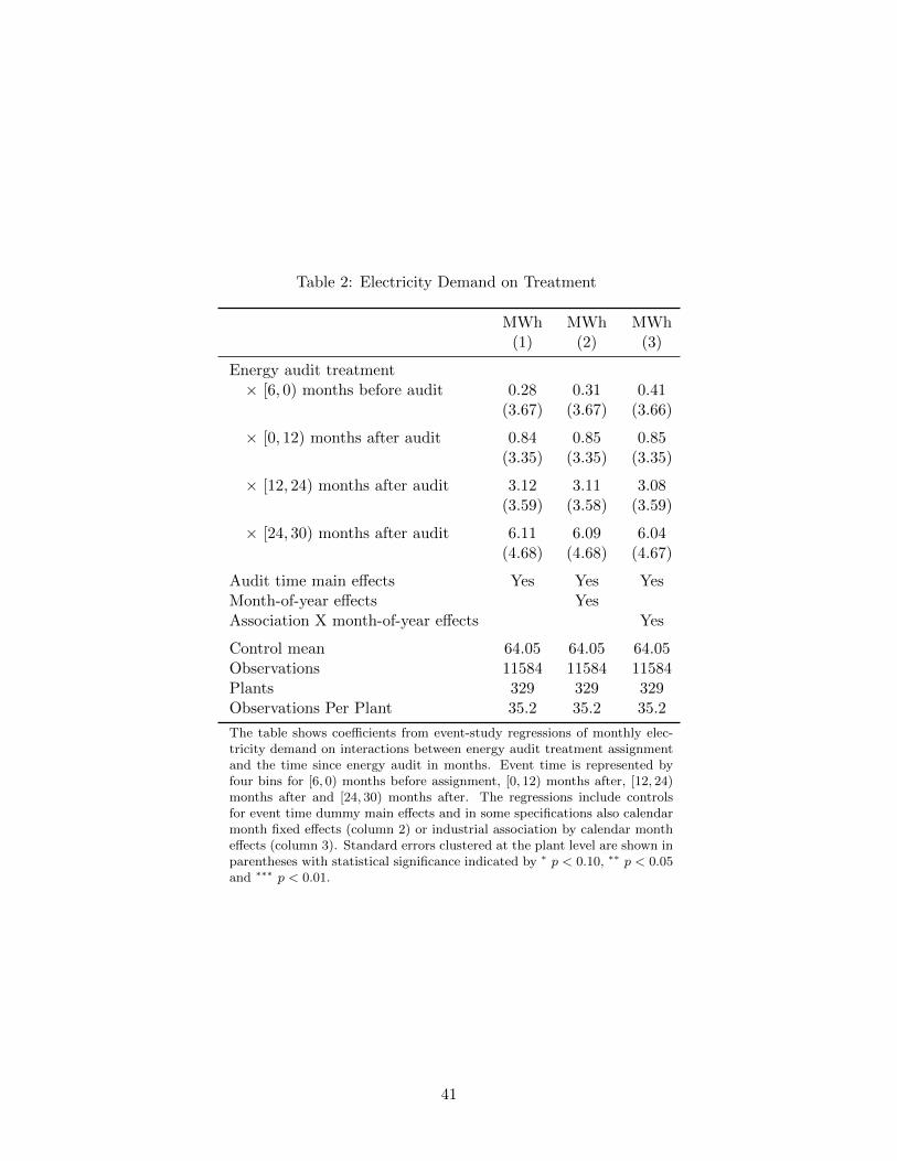
Table 2: Electricity Demand on Treatment
MWh MWh MWh(1) (2) (3)
Energy audit treatment× [6, 0) months before audit 0.28 0.31 0.41
(3.67) (3.67) (3.66)
× [0, 12) months after audit 0.84 0.85 0.85(3.35) (3.35) (3.35)
× [12, 24) months after audit 3.12 3.11 3.08(3.59) (3.58) (3.59)
× [24, 30) months after audit 6.11 6.09 6.04(4.68) (4.68) (4.67)
Audit time main effects Yes Yes YesMonth-of-year effects YesAssociation X month-of-year effects Yes
Control mean 64.05 64.05 64.05Observations 11584 11584 11584Plants 329 329 329Observations Per Plant 35.2 35.2 35.2
The table shows coefficients from event-study regressions of monthly elec-tricity demand on interactions between energy audit treatment assignmentand the time since energy audit in months. Event time is represented byfour bins for [6, 0) months before assignment, [0, 12) months after, [12, 24)months after and [24, 30) months after. The regressions include controlsfor event time dummy main effects and in some specifications also calendarmonth fixed effects (column 2) or industrial association by calendar montheffects (column 3). Standard errors clustered at the plant level are shown inparentheses with statistical significance indicated by ∗ p < 0.10, ∗∗ p < 0.05and ∗∗∗ p < 0.01.
41

Table 3: Physical Efficiency and Capacity Utilization by Treatment Status
Efficiency Hours used per day(1) (2)
Panel A. All SystemsEnergy audit treatment (=1) 0.0848 1.115∗∗
(0.0650) (0.493)
Control mean 0.0 16.7Observations 2175 2134
Panel B. BoilerEnergy audit treatment (=1) 0.287∗ 1.922∗
(0.166) (1.142)
Control mean -0.1 16.3Observations 292 283
Panel C. MotorsEnergy audit treatment (=1) -0.0762 0.801
(0.0786) (0.570)
Control mean 0.0 17.0Observations 1570 1544
Panel D. Jet-Dyeing Machines (Textile Plants Only)Energy audit treatment (=1) 0.142 1.100
(0.250) (1.157)
Control mean -0.0 19.4Observations 128 128
Panel E. Reaction Vessels (Chemical Plants Only)Energy audit treatment (=1) 0.152 0.965
(0.360) (2.256)
Control mean -0.0 13.5Observations 185 179
The table shows regressions of the physical efficiency and hours of use ofpieces of equipment within plants on energy audit treatement status. Physicalefficiency is measured with a standardized index of efficiency composed ofthe average of standardized physical efficiency measures, such as the presenceof insulation or the external temperature of an insulated vessel, where eachstandardized measure is signed so that efficiency is monotonically increasing inthe index. These measures are recorded at the level of the piece of equipmentand so multiple measures may be available per plant. Hours of operation areobtained by asking plant managers or staff how often different equipment isrun. Regressions include baseline electricity demand strata and controls forenergy manager treatment assignment. Standard errors, clustered at the plantlevel, are in parentheses, with statistical significance marked by * p < 0.10,** p < 0.05 and *** p < 0.01.
42

Table 4: Plant Sales and Inputs by Treatment Status
Control Treatment T − C(1) (2) (3)
Sales (USD ’000s) 2036.4 2288.1 251.7[2176.3] [3456.2] (399.8)
103 108 211
High-skill labor (USD ’000s) 28.0 48.5 20.5∗∗∗
[54.3] [81.9] (7.62)169 160 329
Low-skill labor (USD ’000s) 151.3 153.8 2.52[253.8] [222.1] (26.4)
169 160 329
Capital (USD ’000s) 106.0 158.3 52.3∗
[125.0] [283.7] (27.9)125 115 240
Materials (USD ’000s) 586.6 631.6 45.0[764.7] [787.0] (99.7)
130 113 243
Energy (USD ’000s) 368.3 440.2 71.9[321.0] [409.7] (58.1)
89 69 158
The table reports factors of production from the endline survey. Sales, high-skill labor, low-skill labor, capital and materials are responses to questions,asked of the plant owner or manager, on the total value of those inputsused in the last complete fiscal year (2011-12). The capital value shownin the table is the estimated capital input rent, based on multiplying thesurvey answer for the plant’s total market value of capital by an assumedcapital rental rate of 0.15. The energy input is calculated based on thesum of fuel bills, from survey responses, and electricity consumption, fromadministrative data on utility bills, aggregated over the same period. Inputsand sales are shown for all plants reporting each measure with the samplesize listed separately for each variable. Energy input is shown in the tableonly for plants that reported both their electricity and fuel expenses. Thefirst two columns in the table show the means of each factor for the controland treatment groups, respectively, and the last column the difference inmeans across groups. In the third column standard errors are shown inparentheses and the statistical significance of differences is marked by * p< 0.10, ** p < 0.05 and *** p < 0.01.
43

Table 5: Audit Treatment Effects on Employment
Managers Technical Workers
Number Pay Number Pay Number Pay(1) (2) (3) (4) (5) (6)
Energy audit 0.880∗ 8.478∗∗ 2.989∗∗ 14.92∗∗ 6.047 1.139treatment (=1) (0.515) (4.041) (1.361) (6.247) (14.66) (29.96)
Control mean 2.4 12.9 6.0 21.5 88.6 152.5Observations 297 264 309 277 313 286
The table shows the effect of treatment on employment in the endline survey. The endline survey askedthe plant owner or manager about the total number of people employed in different categories as well astheir total annual pay. Managers are “Management (at plant)” employees; technical staff are “Technicalor supervisory (at shop floor, excluding management)” and workers are “Workers (laborers at shopfloor).” Each pair of adjacent columns pertains to one of these three employee types. For each type,the two columns report the coefficient on audit treatment in a regression of the number and total payof those employees on audit treatment and a constant. Total pay is measured in USD ’000s per annum.Statistical significance is denoted by * p < 0.10, ** p < 0.05 and *** p < 0.01.
Table 6: Audit Treatment Effects on Investment
Total capital rental Efficient capital(Endline, USD ’000s) (Endline, USD)
(1) (2) (3) (4) (5) (6)
Energy audit 51.25∗ 49.07∗ 54.55∗ 160.0 128.3 206.2treatment (=1) (28.53) (26.51) (32.05) (209.8) (203.9) (248.0)
Audit treatment (=1) × 0.304∗∗ 0.627Employment at baseline (0.149) (2.019)
Employment at baseline 0.481∗∗∗ 2.133∗∗
(0.0757) (0.975)
Audit treatment (=1) × -4.287∗∗∗ -20.17Projected payback (months) (1.591) (12.72)
Control mean 105.35 105.35 105.35 762.18 762.18 762.18Observations 242 242 242 329 327 329
The table shows regressions of endline plant capital on audit treatment status and baseline plant andaudit characteristics. There are two measures of plant capital. Total capital rental corresponds to therental value of total endline plant capital at a 0.15 rental rate. Efficient capital is the capital investedspecifically in a list of energy-efficiency upgrades, based on the most common energy-efficiency measuresrecommended during audits across all treated plants. Plants were asked about investments in these specificefficiency measures regardless of whether that particular plant received an audit or not. Projected paybackis the number of months until the undiscounted projected value of energy savings will exceed the cost ofa recommended investment for a plant and is therefore inversely related to returns. Projected payback ismeasured only for plants audited so the specifications with projected payback as a control variable alsohave a control dummy (suppressed) for whether projected payback is missing. Standard errors are inparentheses with statistical significance indicated by ∗ p < 0.10, ∗∗ p < 0.05 and ∗∗∗ p < 0.01.
44

Table 7: Production Function Estimates
Textile Chemical Both(1) (2) (3)
∆ 1.059 1.096 1.126(0.051) (0.396) (0.089)
σH 0.027 0.016 0.019(6.545) (13.438) (3.356)
σE 1.059 2.646 1.827(2.175) (7.248) (1.233)
πH 0.063 0.991 0.347(28.391) (62.259) (5.827)
πK 0.936 0.001 0.652(29.923) (7.047) (5.324)
πE 0.370 0.114 0.288(0.024) (0.011) (0.014)
α 0.328 0.052 0.226(0.023) (0.008) (0.019)
µA 7.536 6.499 7.013(11.365) (38.029) (5.023)
σA 0.058 0.130 0.141(0.118) (0.073) (0.191)
φ 0.85 0.85 0.85Over-id p-value 0.450 0.916 0.644Observations 130 166 296
The table provides estimates of the plant production function.The first two columns give estimates for the textile and chem-ical sectors and the third for both sectors together. Each setof estimates uses a generalized method of moments estimator tomatch input demands in the treatment and control groups. Thep-value is from a test of the over-identifying restrictions of themodel based on the GMM criterion where the test statistic isdistributed χ2
11−9.
45

Table 8: Social Surplus Under Productivity Subsidies or an Energy Tax
Energy-efficiencyBaseline Direct Medium- Pigouvian Difference
term tax (4)-(3)(1) (2) (3) (4) (5)
A. TextileEnergy expenditure 535.35 505.65 591.26 505.65 -85.61Profit 335.92 365.62 371.29 323.87 -47.41Social surplus (low social cost) -28.93 21.01 -31.67 -20.74 10.93Social surplus (high social cost) -393.78 -323.60 -434.62 -365.35 69.27
B. ChemicalEnergy expenditure 45.50 41.53 54.85 41.53 -13.32Profit 76.07 80.04 80.58 74.76 -5.82Social surplus (low social cost) 45.07 51.74 43.20 46.45 3.26Social surplus (high social cost) 14.06 23.44 5.82 18.15 12.33
C. BothEnergy expenditure 183.67 163.05 232.36 163.05 -69.31Profit 133.51 154.13 158.42 126.25 -32.18Social surplus (low social cost) 8.34 43.01 0.07 15.13 15.06Social surplus (high social cost) -116.83 -68.10 -158.29 -95.99 62.30
The table shows energy expenditure, profits and social surplus under alternative energy policy regimes.All numbers in the table are in USD ’000s per plant. The baseline regime (column 1) represents thecontrol group without energy-efficiency subsidies or taxes. Direct (column 2) endows plants with energy
productivity ∆ = ∆1 but does not allow inputs to adjust, whereas medium-term (column 3) provides thesame energy productivity and allows inputs to adjust. Finally, Pigouvian tax gives the plant responseunder an energy tax calibrated for plant energy demand to match the column 2 level of energy demand.The rows give values for energy expenditure, plant profit and social surplus, where surplus is reportedseparately for low and high assumptions on the social cost of energy use.
46

Appendix A [NOT FOR PUBLICATION]
A Data Appendix
This section contains supplementary information on the experimental design and the mea-
sures recommended in energy audits.
A.1 Context
Many unilateral and multilateral aid agencies are active in subsidizing energy-efficiency
initiatives for Indian manufacturing plants. Table A1 describes initiatives active around the
time of the experiment studied in this paper. Most initiatives are funded by foreign donors
and administered by the Government of India through the Small Industries Development
Bank of India (SIDBI) and the Bureau of Energy Efficiency (BEE).
Table A1: Industrial Energy-Efficiency Initiatives in India
Who? When? Name? What?
BEE,SIDBI
2012-2013 World Bank – GlobalEnvironment Facility
Energy audits and capacity buildingin 5 industrial clusters
SIDBI,KfW
2012 Financing Energy Effi-ciency Projects in theMSME Sector
Subsidised lending pass-through ofUSD 70m loan for MSME units
BEE 2010-2011 BEE Small- andMedium-EnterpriseProgram
Energy audits, technology identifi-cation, capacity building for over4,000 units in 35 clusters
SIDBI,JICA
2010-2011 SIDBI FinancingScheme for MSMEs
Subsidised lending pass-through ofUSD 330m loan for MSME unitswith 10% savings potential
US AID,BEE
2006-2009 Energy Conservationand CommercializationProject, Phase III
Feasibility studies, technology de-velopment, select investment-gradeaudits for four SME clusters
A.2 Experimental Integrity
This subsection provides further details about the experimental design and compliance to
extend the discussion in Section II.D.
Table A2 shows the interest in plants contacted to participate in the experiment. The
universe of plants comprised the members of textile and chemical industrial associations
in several cities of Gujarat. Energy consultants contacted randomly sampled members to
solicit their interest in possibly receiving energy consulting services. Table A2 shows the
47

Appendix A [NOT FOR PUBLICATION]
replies of plants to this outreach, and is discussed in the text. The number of interested
plants is larger than the sample because further screening criteria were applied to restrict
the sample of interested plants.
Table A2: Plant Interest in Energy Consulting
Plant interestNumber Percent
(1) (2)
Interested 490 53.0Already have consultant 38 4.11Energy not a large cost 40 4.32Scope of savings not large 50 5.41Other 307 33.2Total 925 100
The table shows interest in joining the experimental sample, assolicited by energy consultants, amongst plants in the larger pop-ulation of membership rolls in local industrial associations.
Plants that declined interest did not complete the baseline survey and so it is difficult
to gauge how screening on interest affected the composition of the sample. As described
in Section II.B, Table A3 compares the characteristics of plants that were and were not
intersted in administrative data available for a subsample of plants.
I collected administrative data on industrial registrations from the Industries Commis-
sioner, Government of Gujarat. Registration data includes details such as the capital stock
and employment of plants, but has several limitations: it is only available for plants that
register, is typically out of date, and it may be distorted if plants do not report truthfully
to the government. Appendix Table A3 compares plant characteristics, in the registration
data, for plants that were interested in the experiment versus not, among the 206 solicited
plants that could be matched to this data set. The rate of interest is higher amongst
matched plants, at 75% instead of 53%, presumably because registered plants tend to be
larger. Within the matched plants, most observable characteristics are similar, but inter-
ested plants have a larger total capital stock, by USD 101 thousand (standard error USD
63 thousand).
Table A4 describes the cross-cutting experimental design and compliance. Panel A
describes the treatment assignments: plants were assigned to the energy audit treatment
or control groups, and, conditional on completing an energy audit, were assigned to the
48

Appendix A [NOT FOR PUBLICATION]
Table A3: Selection into the Sample
Sample mean [sd]Interested Not Difference
Electricity load in kW 65.9 60.4 5.53[67.4] [78.0] (11.3)
Capital (USD ’000s) 231.7 130.6 101.0[445.0] [165.5] (63.2)
Capital, plant (USD ’000s) 96.5 77.0 19.5[184.8] [111.1] (27.2)
Capital, equipment (USD ’000s) 7.72 7.39 0.33[41.0] [36.5] (6.41)
Capital, building (USD ’000s) 76.8 29.1 47.6[219.3] [40.6] (30.6)
Capital, land (USD ’000s) 50.6 17.2 33.5[246.4] [14.8] (34.3)
Employment 15.2 13.2 1.91[13.9] [11.4] (2.14)
Observations 154 52
The table compares observable characteristics of plants interested or not inter-ested in participating the experiment in data from industrial registrations withthe state of Gujarat. Industrial registration data is available for a subset of 206 ofthe 925 plant population fo the experiment due to partial registration and limitedmatching. Registration data gives characteristics as reported to the governmenton establishment of the plant.
49

Appendix A [NOT FOR PUBLICATION]
energy manager treatment. Panel B describes compliance with the experimental treatment
assignments.
Table A4: Experimental Design and Compliance
Control Treatment Total(1) (2) (3)
A. Treatment Assignments
Energy Audit TreatmentEnergy Manager TreatmentTotal 216 219 435
Control 0 81 81Treatment 0 83 83Not assigned 216 55 271
B. Treatment Completion
Energy Audit TreatmentShare of plants doing energy audit 0.12 0.79 0.67∗∗∗
(0.035)
Energy Manager TreatmentShare of plants using energy manager 0.12 0.35 0.23∗∗∗
(0.064)
The table shows the experimental design and treatment assignments, in Panel A, and theactual completion of energy audits or use of energy managers, in Panel B. In Panel A thecolumns indicate energy audit treatment assignment and the rows energy manager treatmentassignment and each cell reports the number of plants assigned to that combination of treat-ments. Plants are assigned to the energy manager treatment conditional on completing theenergy audit treatment and expressing interest in implementation. In Panel B the columnsindicate treatment assignment status for the energy audit treatment, in the first row, andthe energy manager treatment, in the second row. Each table entry gives the share of plantscompleting the treatment, or similar consultancy outside the experiment, conditional on thetreatment assignment shown by the column.
Table A5 describes attrition from the experiment. Of the total sample of 435 plants
at baseline, 334 plants completed the endline survey. Roughly half of those that did not
complete the survey had closed down, and the other half refused the survey. The text
discussed the rate of refusal, which was primarily due to data confidentiality concerns. The
data sought for the endline was relatively more invasive than the data collected in the brief
baseline.
Table A6 compares the rate of attrition across treatment arms. A primary concern
would be whether energy consulting increased plant profitability and therefore altered the
selection of plants that remained open at the end of the experiment. There is no evidence
for such differential selection on treatment status: overall, control plants are slightly (not
50

Appendix A [NOT FOR PUBLICATION]
Table A5: Attrition in the Endline Survey
N %
Surveyed 334 76.8Not surveyed 101 23.2
Shut down/Sold off 42 9.7Refused 52 12.0Other 7 1.6
Total 435 100.0
Shut down/sold off includes plants that were permanentlyclosed and plants that were temporarily closed during re-peated survey visits. Refused includes plants that were op-erating at the time of the visit, but that refused to respond.Other includes plants that moved or that could not be con-tacted.
significantly) more likely to be surveyed at endline, and the rate of plant closure in the
control and treatment groups is nearly identical.
Table A6: Endline Attrition by Treatment Status
Treatment Control Difference
Surveyed 0.744 0.792 -0.048[0.437] [0.407] (0.040)
Shut down/Sold off 0.096 0.097 -0.001[0.295] [0.297] (0.028)
Refused 0.142 0.097 0.045[0.349] [0.297] (0.031)
Other 0.018 0.014 0.004[0.134] [0.117] (0.012)
Observations 219 216
Shut down/sold off includes plants that were permanently closed andplants that were temporarily closed during repeated survey visits. Re-fused includes plants that were operating at the time of the visit, butthat refused to respond. Other includes plants that moved or thatcould not be contacted.
A.3 Audit Recommendations and Projected Returns
Energy consultants recommended 1,959 measures in energy audit reports for 173 treatment
plants that completed audits. Table A7 characterizes the types of measures recommended.
Each row presents summary statistics for a measure of a different type, or pertaining to a
different system, such as lighting, motors, insulation, heat recovery and so forth. Within
each row, the columns show (1) the share of plants with any recommendation in that cate-
51

Appendix A [NOT FOR PUBLICATION]
gory, (2) the mean number of measures in that category, conditional on a reconmmendation,
(3) the mean and (4) median investment size of a measure, and (5) the median return on a
measure of that type.
Table A7: Energy Audit Measures Recommended and Projected Returns
Measure Investment ReturnPrevalence Size (USD) (%)
Plant NumberShare if Any Mean Median Median
(1) (2) (3) (4) (5)
Total 1.00 12.04 1249.06 361.11 104Lighting 0.82 1.57 1304.40 305.56 94Motor sizing / efficiency 0.78 10.13 1029.29 361.11 101Insulation 0.46 2.17 476.50 260.00 175Electricity Tariff 0.42 1.40 579.40 253.33 154Heat Recovery 0.39 1.27 5956.81 5581.51 220Maintenance / Other 0.23 1.38 1083.40 536.11 1601Automation 0.10 1.06 2017.35 666.67 155Compressors 0.09 1.20 3495.29 1111.11 80Drives / belts / pulleys 0.07 1.91 2666.51 2000.00 71
The table shows characteristics of investments recommended in energy audits of treatment plants.The rows give the type of equipment or system that the measure involves, and the columns givestatistics on the prevalence (columns 1 and 2), investment cost (columns 3 and 4) and returns(column 5) on these measures. A total of 1,959 measures have non-zero investment and so finitereturns.
Figure A1 shows the distribution of investment ticket sizes for the measures described in
Table A7, omitting measures that do not require any capital investment. The distribution
of investments is right-skewed but most ticket sizes are very small relative to the capital
stock of sample plants.
52

Appendix A [NOT FOR PUBLICATION]
Figure A1: Capital Needed for Energy-Efficiency Investments
010
2030
Perc
ent
0 2000 4000 6000 8000 10000Investment required for energy-efficiency measure (USD)
The figure shows the distribution of investment costs for measures recommended in energy audits in theenergy audit treatment group of plants. Each bin is USD 200 wide and the distribution is truncated at the97.5th percentile (USD 11,111) for clarity. The investments are for 1,959 different measures recommendedto 173 treatment plants.
53

Appendix B [NOT FOR PUBLICATION]
B Model Appendix
B.1 Plant input demands
The plant’s problem yields a system of five non-linear equations given by the first-order
conditions for each input. The solution of this system yields demands for each factor in
terms of energy:
Mi =
(1− αα
pLpM
)Li = AMLLi
Li =
(∆ρ2i
π31− π3
pLpE
1
αA
(1−α)(α−ρ2)ML
) 1ρ2−1
Ei = ALE(∆i)Ei
X1i =(π3∆
ρ2i + (1− π3)(A1−α
MLALE(∆i))ρ2)1/ρ2
Ei = AX1E(∆i)Ei
Ki =
(π1π2
pKpH
) 1ρ1−1
Hi = AKHHi
Hi =
((1− π1 − π2)π3
π1
pHpE
AX1E(∆i)ρ1−ρ2∆ρ2
i
) 1ρ1−1
Ei = AHE(∆i)Ei.
The ratios of materials to unskilled labor demand and of capital to skilled labor demand do
not depend on energy productivity, by virtue of the assumed form of the production function.
This specification choice is deliberate in order to match the reduced-form experimental
results for input demand.
If we substitute these demands into the first-order condition for energy, we can solve for
energy demand:
E = A1
1−φi
[∆ρ2i
φ
pE(π1AHE(∆i)
ρ1 + π2(AKHAHE(∆i))ρ1 + (1− π1 − π2)AX1E(∆i)
ρ1)φ/ρ1−1
×(1− π1 − π2)π3Aρ1−ρ2X1E
] 11−φ
= AE(∆i)A1
1−φi .
The remaining input demands can then be calculated through their dependence on energy
54

Appendix B [NOT FOR PUBLICATION]
demand.
Ei = AE(∆i)A1
1−φi
Mi = AMLLi = AMLALE(∆i)Ei
Li = ALE(∆i)Ei
X1i = AX1E(∆i)Ei
Ki = AKHHi = AKHAHE(∆i)Ei
Hi = AHE(∆i)Ei.
B.2 Mean input demand moments
The above demands are for individual plants with total factor productivity Ai and energy
productivity ∆i. We derive moments for mean input demands by parameterizing the het-
erogeneity across plants. Alternately, this step could be omitted to fit control and treatment
input demands for a representative plant in each treatment arm.
We assume the distribution of total factor productivity is log normal
logAi ∼ N (µA, σA).
We additionally assume that each input observed is the plant’s input choice plus a mea-
surement shock
Xi = Xi + εXi, E[εXi|Xi] = 0.
The measurement error εXi is assumed to have mean zero conditional on inputs and to be
conditionally independent across factors given a vector of input demands.
The main identification assumption is that control plants have energy productivity ∆i =
∆0 ≡ 1 and treatment plants energy productivity ∆i = ∆1, to be estimated.
55

Appendix B [NOT FOR PUBLICATION]
The system of measured demands, with measurement error, can be written:
E = AEA1
1−φi + εEi
Mi = AMLALEEi + εMi
Li = ALEEi + εLi
Ki = AKHAHEEi + εKi
Hi = AHEEi + εHi.
By the law of iterated expectations
E[E] = E[AEA1
1−φi ]
E[Mi] = E[AMLALEEi]
E[Li] = E[ALEEi]
E[Ki] = E[AKHAHEEi]
E[Hi] = E[AHEEi].
The input demands are log-normal. Let the level of the input demand for Xi be A1
1−φi AX .
Then logXi = logAXE(∆) + logAE(∆) + 11−φ logAi. Hence Xi is distributed log-normally
with
µX = logAXE(∆) + logAE(∆) +1
1− φµA
= logAX(∆) +1
1− φµA
σX =1
1− φσA.
Where AX ≡ AXEAE . The expected value of any input demand X therefore depends on
the distribution of productivity and the factor that relates demand for X to demand for E.
E[Xi] = exp(µX(∆) + σ2X/2
)= exp
(logAX(∆) +
1
1− φµA +
(1
1− φσA
)2
/2
).
56

Appendix B [NOT FOR PUBLICATION]
Hence for all five input demands
E[E(∆i)] = AE(∆) exp
(1
1− φµA +
(1
1− φσA
)2
/2
)E[M(∆i)] = AMLALEE[E(∆i)]
E[L(∆i)] = ALEE[E(∆i)]
E[K(∆i)] = AKHAHEE[E(∆i)]
E[H(∆i)] = AHEE[E(∆i)].
These expected input demands, conditioned on ∆ = ∆0 ≡ 1 and ∆ = ∆1, provide ten
moments, for the five input demands in two treatment conditions.
From the input demand moments alone, we cannot separately identify the mean and vari-
ance of log productivity. Therefore we add an additional moment based on the covariance
of input demands. Since input factor measurement errors are mean independent, covariance
of input factors is due to variance in total factor productivity, rather than measurement
error. Take the covariance of energy and labor as an example.
Cov(Ei, Li) = Cov(Ei + εEi, Li + εLi)
= Cov(Ei, Li)
= Cov
(AE(∆)A
11−φi , ALE(∆i)AE(∆i)A
11−φi
)= ALE(∆i)AE(∆i)
2Cov
(A
11−φi , A
11−φi
)= ALE(∆i)AE(∆i)
2Var
(A
11−φi
).
The variance of a log normally distributed variable with log mean µ and log standard
deviation σ is given by (exp(σ2)− 1) exp(2µ+ σ2). Hence in this case
Var
(A
11−φ
i
)=
[exp
((1
1− φ
)2
σ2A
)− 1
]exp
(2
1
1− φµA +
(1
1− φ
)2
σ2A
).
I use this expression to calculate the moment for the expected covariance of energy and
labor demands.
57

Appendix B [NOT FOR PUBLICATION]
B.3 Robustness of Production Function Estimates
The estimates in Table 7 calibrate revenue returns to scale to equal φ = 0.85 ≈ (ε−1)/ε× φ
for ε = 10 and physical returns to scale φ = 0.95. This value is between the range of values
from ε = 4, φ = 1 to ε = 10, φ = 1 used by Allcott, Collard-Wexler and O’Connell (2016)
for manufacturing plants in India.
Table B8 shows estimates of the production function for the endpoints of their range of
values as a robustness check. At the higher end, we consider φ = 0.90 = (ε − 1)/ε × φ for
ε = 10 and physical returns to scale φ = 1.00. At the lower end, φ = 0.70 ≈ (ε− 1)/ε× φ
for ε = 4 and physical returns to scale φ = 0.95.
The calibrated value of φ affects parameter estimates in an intuitive way. Consider the
textile sector. In the main estimates with φ = 0.85 from Table 7, we estimate ∆1 = 1.059.
With a lower φ = 0.70, in Table B8 column 1, the estimate rises to ∆1 = 1.164, and with
a higher φ = 0.95, in column 4, the estimate falls to ∆1 = 1.035. The higher is φ, the
less concave is revenue production, and therefore the smaller needs to be any increase in
energy productivity in order to rationalize the observed increases in input demands. By
contrast, if φ is low, for example because the elasticity of demand is smaller in magnitude,
then revenue production is concave and a large increase in energy productivity is needed to
rationalize the observed changes in input demand.
58

Appendix B [NOT FOR PUBLICATION]
Table B8: Production Function Estimates: Robustness to Scale Parameter
Textile Chemical Both Textile Chemical Both(1) (2) (3) (4) (5) (6)
∆ 1.164 1.234 1.337 1.035 1.060 1.077(0.135) (1.085) (0.255) (0.031) (0.241) (0.053)
σH 0.025 0.016 0.017 0.031 0.044 0.024(2.600) (7.597) (1.510) (10.437) (19.896) (5.010)
σE 1.005 1.728 1.348 1.132 3.581 2.319(0.813) (3.343) (0.508) (3.581) (11.300) (1.976)
πH 0.053 0.984 0.336 0.081 0.386 0.343(11.325) (56.644) (2.310) (43.008) (313.484) (7.117)
πK 0.946 0.001 0.663 0.917 0.062 0.655(12.205) (3.938) (1.813) (48.591) (28.094) (3.754)
πE 0.371 0.115 0.288 0.370 0.114 0.287(0.024) (0.014) (0.017) (0.023) (0.008) (0.011)
α 0.328 0.052 0.226 0.328 0.052 0.226(0.023) (0.008) (0.019) (0.023) (0.008) (0.019)
µA 7.751 6.646 7.173 7.479 6.508 6.976(3.858) (17.418) (2.038) (19.367) (12.332) (8.706)
σA 0.117 0.260 0.281 0.039 0.087 0.094(0.024) (0.057) (0.017) (0.077) (0.033) (0.038)
φ 0.70 0.70 0.70 0.90 0.90 0.90Over-id p-value 0.500 0.921 0.740 0.438 0.915 0.617N 130 166 296 130 166 296
The table provides estimates of the production function specified by equation 1. The first twocolumns give estimates for the textile and chemical sectors and the third for both sectors together.Each set of estimates uses a generalized method of moments estimator to match input demands inthe treatment and control groups. The p-value is from a test of the over-identifying restrictions ofthe model based on the GMM criterion where the test statistic is distributed χ2
11−9 (Newey andMcFadden, 1994). The first three columns show the estimates with an assumed value of φ = 0.70and the next three with a value of φ = 0.90, both to be compared with the baseline value of φ = 0.85.
59