NBER WORKING PAPER SERIES

ROBUSTNESS OF PRODUCTIVITY ESTIMATES

Johannes Van Biesebroeck

Working Paper 10303http://www.nber.org/papers/w10303

NATIONAL BUREAU OF ECONOMIC RESEARCH1050 Massachusetts Avenue

Cambridge, MA 02138February 2004

I would like to thank Mel Fuss, Robert Gagné, Marc Melitz, Ariel Pakes, Peter Reiss, Chad Syverson, FrankWolak, and participants at the NBER 2002 Summer Institute and SITE 2003 for comments. All remainingerrors are my own. Financial support from the Connaught Fund is gratefully acknowledged. The viewsexpressed herein are those of the authors and not necessarily those of the National Bureau of EconomicResearch.

©2004 by Johannes Van Biesebroeck. All rights reserved. Short sections of text, not to exceed twoparagraphs, may be quoted without explicit permission provided that full credit, including © notice, is givento the source.

Robustness of Productivity EstimatesJohannes Van BiesebroeckNBER Working Paper No. 10303February 2004JEL No. D24, C13, C14, C15, C43

ABSTRACT

Researchers interested in estimating productivity can choose from an array of methodologies, each

with its strengths and weaknesses. Many methodologies are not very robust to measurement error

in inputs. This is particularly troublesome, because fundamentally the objective of productivity

measurement is to identify output differences that cannot be explained by input differences. Two

other sources of error are misspecifications in the deterministic portion of the production technology

and erroneous assumptions on the evolution of unobserved productivity. Techniques to control for

the endogeneity of productivity in the firm's input choice decision risk exacerbating these problems.

I compare the robustness of five widely used techniques: (a) index numbers, (b) data envelopment

analysis, and three parametric methods: (c) instrumental variables estimation, (d) stochastic

frontiers, and (e) semiparametric estimation. The sensitivity of each method to a variety of

measurement and specification errors is evaluated using Monte Carlo simulations.

Johannes Van BiesebroeckDepartment of EconomicsUniversity of Toronto150 St. George StreetToronto, ON M5S 3G7CANADAand NBERjovb@chass.utoronto.ca

1 Motivation

Accurate measurement is at the heart of productivity comparisons. Fundamentally, the

objective is to identify output differences that cannot be explained by input differences.

To perform this exercise, one needs to observe inputs and outputs accurately and control

for the input substitution that the production technology allows. Problems can arise from

misspecifications in the deterministic or stochastic portion of the production technology and

from measurement errors in the data.

Firms use different input combinations to produce one unit of output because their

technology differs, which I label productivity differences, or because they face different factor

price, which leads firms to pick different points on the production frontier.1 The extent to

which one input can be substituted for another is determined by the shape and position of

the production function—or any other representation of technology—and is naturally not

observable. Methodologies to estimate productivity differ by the mix of statistical techniques

and economic assumptions they employ to control for input substitution. Misspecifications

in the deterministic part of the production function or in the statistical model underlying the

evolution of unobserved productivity will have repercussions on the productivity estimates.

Mismeasurement can result, among other things, from unobserved quality or price

differences, aggregation problems, recall errors in surveys, or incompatibilities in reference

period for output and inputs. The effect on productivity estimates obviously depend on

the estimation method. For example, Griliches and Hausman (1986) argue that while first-

differencing is useful to control for unobserved firm-specific effects, identification based on

thinner slices of the data are more vulnerable to measurement errors. Solutions exist for

dealing with well-defined forms of measurement error, but they are rarely used in practice.

One of the goals in this paper is to verify how sensitive different methods for productivity

measurement are to different forms of measurement error.

I evaluate the robustness to misspecification and measurement errors for five popular

1Some authors have argued that some of the output shortfall relative to the best practice frontier is theresult of inefficiency. I still classify such shortfall as productivity differences, to remain consistent with aprofit maximizing model of the firm. Lower output might be caused by differences in production technology,unmeasured inputs, or quality differences in outputs. See Stigler (1976) for a more elaborate motivation.

2

methodologies. The first two methods, index numbers and data envelopment analysis, are

very flexible in the specification of technology, but do not allow for unobservables, making

the effect of measurement error completely unpredictable. The three parametric methods

calculate productivity from an estimated production function. In the simplest linear regres-

sion model, measurement error in the dependent variable has no effect on the consistency of

least squares estimates, while errors in the independent variables biases coefficient estimates

downwards. For most production function estimators, the effects are not so straightforward,

because more complicated estimators are devised to deal with the simultaneity of produc-

tivity and input choice. Moreover, the principal interest is in the residual of the production

function, which is always affected. I evaluate the robustness of both productivity level and

growth estimates using simulated data.2

In the next section, I start with some background on productivity measurement and,

subsequently, I introduce the different methodologies. An attempt is made to present the

general idea of each methodology in a consistent framework and convey the distinctive fea-

tures as briefly as possible. Links to the literature for more extensive information and

discussion are provided. Section 3 describes the data generation process, starting from the

input choices of a profit maximizing representative firm. For each set of assumptions on the

evolution of productivity that have been considered in the literature, I solve analytically or

numerically for the optimal investment policy. In Section 4, the sensitivity of the different

estimation methodologies to variations of three elements of the data generating process is

evaluated. First, different assumptions are used to model the unobserved productivity term.

Second, measurement error of varying size is added to output and inputs. Third, the returns

to scale of the production technology is varied. Lessons to take away from these exercises

are summarized at the end.

2For a related study that uses manufacturing data from Colombia to compare the different methodologies,see Van Biesebroeck (2003b).

3

2 Measuring Productivity

In plain English, one firm is more productive than another if it is able to produce the same

outputs with less inputs or if it produces more outputs from the same amount of inputs.

Similarly, a firm has experienced positive productivity growth if outputs have increased more

than inputs or inputs have decreased more than outputs. The comparison becomes more

interesting if one firm (or the same firm in one of the comparison periods) uses more of one

input, while the other relies more on a second input. In that case, it becomes necessary

to specify a transformation function that links inputs to outputs. Since a firm’s input

substitution possibilities are determined by the technology it employs, each productivity

measure is only defined with respect to that specific production technology.

Measuring productivity necessarily involves decomposing differences in the input-

output combinations into shifts along a production frontier and shifts of the frontier itself.

In Figure 1, two production plans, P0 and P1, are compared in input space and the frontier

is represented by the unit isoquant. Part of the difference, from P0 to 1, is a shift along

the frontier, exploiting the input substitution the technology allows. The remainder of the

difference, from 1 to P1, is an actual shift of the frontier, which is counted as technical change

or productivity growth. In this example, an intuitive measure of P0’s productivity relative

to P1 is 0P1

01.

If the shape of the unit isoquant in Figure 1 is not known, it can be estimated paramet-

rically if one is willing to make functional form assumptions. Simultaneity of productivity

and input choice is the main econometric issue. I discuss three different estimators that

control for it in Section 2.3.

Another approach is to rely on index number theory, which is discussed in Section

2.2. If the first order conditions for input choices hold, the factor price ratio will equal the

slope of the input isoquant, which determines input substitution possibilities. Taking the

average of the ratio for both production plans that are compared, it is possible to control

for input differences without having to estimate anything. Figure 2 compares the same two

production plans as before. The reference production plan (P0) uses more labor (less capital)

which will be accounted for in proportion to the average labor share (capital share) in costs.

4

Figure 1: Decomposing shifts along the frontier from a shift of the frontier: parametrically

L

x P0

Unit isoquant

1xP1

K

A third, nonparametric approach, constructs a piece-wise linear isoquant to maximize

the productivity for P1, without allowing any other plan to lie below the isoquant. The

relevant section of the isoquant, connecting P2 and P3 in Figure 3, implicitly defines relative

weights for labor and capital. Weights are chosen to maximize productivity for P1, i.e. to

minimize its distance to the isoquant. When evaluating different production plans, different

weights are used, as discussed in Section 2.1.

Using each method, two production plans are compared, which can refer to two

different firms or to a single firm at two different points in time. Productivity measures

can be output- or input-based. Output-based measures provide an answer to the question:

“How much extra output does a firm produce, relative to another firm, conditional on its

(extra) input use?” Input-based measures ask “What is the minimum input requirement

for one firm to produce the same output as another firm?” Under constant returns to scale

both measures will coincide. Most applications limit themselves to a single output and only

calculate output-based measures and I’ll do likewise.3

3In practice, most data sets only contain deflated sales or value added as single output aggregate, implying

5

Figure 2: Decomposing shifts along the frontier from a shift of the frontier:with index numbers

L

x P0 Unit isoquant 0

t0 tmean

t1 x Unit isoquant 1

t0 tmean P1 t1

K

A final restriction is to consider only Hicks-neutral productivity differences. These are

represented by a multiplicative term in the production function, Ait, which differs between

firms and time periods and affects all inputs identically:4

Qit = Ait F(it)(Xit). (1)

The deterministic portion of the technology is represented by the production function F (.).

If the technology is allowed to vary across observations—for the index number and DEA

methods—one has to be explicit which technology underlies the comparison, hence the (it)

subscript.

The productivity of firm i relative to firm j, both at time t, is given by log Ait

Ajt. For

productivity level, multilateral comparisons are more common, using the average productiv-

some aggregation of products using prices within the firm.4Most studies use a Cobb-Douglas production function, which makes it impossible to identify the factor-

bias of technological change.

6

Figure 3: Decomposing shifts along the frontier from a shift of the frontier: nonparametrically

L

Unit isoquantx P0

x P2

x P1

x P3

K

ity level for all plants in the denominator. In practice, logAit − logAt is most often used

for multilateral productivity comparisons, taking the average of the logarithm. For compa-

rability purpose, I follow this practice. The productivity growth for firm i from t− 1 to t is

measured as log Ait

Ait−1. Rearranging the production function as

logAit

Ajτ

= logQit

Qjτ

− logF (Xit)

F (Xjτ ). (2)

illustrates that productivity is intrinsically a relative concept. The calculation of the last

term in (2)—the ratio of input aggregators—distinguishes the different methods.5

Three broad classes of methodologies are introduced in the following sections. They

are ordered by increasing sensitivity to specification error and decreasing vulnerability to

measurement error, at least that is the a priori expectation. The Monte Carlo simulations

will confirm or reject these priors and give an idea of the robustness of each method. Readers

familiar with the different methodologies might still find the expositions useful, as estimates

5I dropped the technology subscripts for the input aggregators as different methods use different assump-tions, see below.

7

from different literatures are presented in a unified framework.6

2.1 Data envelopment analysis (DEA)

The first approach to productivity measurement relies on nonparametric estimation tech-

niques using linear programming. The basic method dates back to Farrell (1957) and it was

operationalized by Charnes, Cooper, and Rhodes (1978).7 No particular production function

is assumed. Instead, productivity equals the ratio of a linear combination of outputs over a

linear combination of inputs. Weights are chosen optimally for the unit under consideration,

with the restriction that the efficiency of all (other) observations cannot exceed 100% when

the same weights are applied to them. Observations that are not dominated are labeled 100%

efficient. Domination occurs when another firm, or a linear combination of other firms, uses

less of all inputs to produce the same outputs or produces more of all outputs using the same

inputs.

Figure 4 provides some intuition for the DEA methodology. It is drawn for a single

input and output, but the intuition is similar for higher dimensional problems as the inputs

and outputs are always aggregated linearly.8 P1 to P5 are production plans of different

firms. The solid line represents the frontier under variable returns to scale. It fits a piece-

wise linear frontier over the extreme points. Four of the five observations lie on the frontier

and are deemed 100% efficient. If the technology is restricted to constant returns to scale,

the frontier is forced to go through the origin and is extrapolated beyond observed data

points, resulting in the dashed line as production frontier. Only P2 is fully efficient in this

case. Imposing constant returns to scale adds a constraint to the problem, restricting the

weights and lowering the maximized objective value—the efficiency.

The distance of each unit to the frontier represents its (in)efficiency. In an input

orientation, efficiency is improved by reducing inputs: a horizontal projecting onto the fron-

6On the measurement front, I abstract from a number of issues that researchers have dealt with. Theseinclude, but are not limited to, the appropriateness of deflated sales as output measure if competition isimperfect; value added versus gross output production functions; the aggregation of heterogeneous inputsand outputs; variations in capacity utilization; and regulated firms.

7More information on the method and applications can be found in Seiford and Thrall (1990).8Because weights to construct the input and output aggregate are chosen optimally for the observation

under consideration, the axes will be different for each comparison unit, with multiple inputs or outputs.

8

Figure 4: Nonparametric production frontiers

QX P4

X P3

X P2 output

input X P5

XP1

0X

tier. In an output orientation, the projection is vertical, increasing output holding inputs

constant. Figure 4 makes clear that under variable returns both orientations yield different

results, as the frontier does not go through the origin and the slope of the segments the unit

gets projected onto might differ.

To obtain the efficiency measures, a linear programming problem is solved separately

for each observation. Input and output weights are chosen to maximize efficiency. The num-

ber of restrictions equals the number of observations, plus sign restrictions on the weights.

For unit 1, the problem amounts to

maxvl,uk

θ1 =

∑Ll=1 vlq1l + v∗∑K

k=1 ukx1k

subject to∑

l vlqil + v∗∑k ukxik

≤ 1 i = 1...N

vl, uk ≥ 0 l = 1...L, k = 1...K,

v∗ ≥ 0 (v∗ = 0 for constant returns to scale),

(3)

i indexes firms, l outputs, and k inputs. The problem is linearized by multiplying both sides

9

of the restrictions by the denominator and normalizing the linear combination of inputs in

the denominator of the objective function to one.9 In practice, most applications solve the

dual problem, where θ1 is chosen directly.10 Setting the slack variable (v∗) to zero enforces

constant returns to scale, which will result in a lower minimized value for θ1.

The efficiency measures θi can be interpreted as the productivity difference between

unit i and the most productive unit: θi = AiAmax

. To obtain a measure comparable to the

ones obtained with other methodologies, I define the relative productivity level as

logADEAi − logA

DEA= log θi −

1

N

N∑i=1

log θi. (4)

Productivity growth is less often measured in the DEA framework. Including the different

firm-years as separate observations in the analysis, it is possible to calculate productivity

growth as

logADEAit − logADEA

it−1 = log θit − log θit−1. (5)

While these transformations are arbitrary, they do not change the ranking of firms, only the

absolute productivity levels and growth rates.

DEA has the advantage that it deals with many outputs in a consistent way and leaves

the underlying technology unspecified, even allowing it to vary across firms. No functional

form or behavioral assumptions are made. While there is no theoretical justification for

the linear aggregation, it is natural in an activities analysis framework. Each firm can be

considered a separate process that is combined with others to replicate the production plan of

the unit under investigation. On the other hand, the flexibility in weighting has drawbacks.

Each firm with the highest ratio for any output-input combination is 100% efficient, as it can

put maximum weight on these factors. Under variable returns to scale, each firm with the

lowest input or highest output level in absolute terms is also fully efficient. The method is

9Without normalization, multiplying all weights by a multiplier does not change the problem in (3).10θ1 gives an input-based efficiency measure for firm 1. Interchanging the roles of inputs and output in (3)

and minimizing the objective function, gives the corresponding output-oriented programming problem. Inthat case, efficiency is given by the inverse of the optimized objective value. The problem is similar to theMalmquist index, see equation (7) later, but instead of assuming a translog input distance function, inputsare aggregated linearly.

10

not stochastic, which makes it sensitive to outliers.11 Because each observation is compared

to all others, measurement error for a single firm can affect all productivity estimates.

2.2 Index numbers (IN)

The second approach to productivity measurement, index numbers, provides a theoretically

motivated aggregation method for inputs and outputs. It remains fairly agnostic on the shape

of the underlying production technology and allows some heterogeneity. Under a number of

assumptions, it is possible to calculate the last term in (2) from observables, without having

to specify or estimate the production function.

The first growth accounting exercise by Solow (1957) used the following total factor

productivity (TFP) growth formula:

logAit

Ait−1

= logQit

Qit−1

− (sLit+sL

it−1

2) log

Lit

Lit−1

− (1− sLit+sL

it−1

2) log

Kit

Kit−1

, (6)

where sLit is the fraction of the wage bill in output or total cost. Diewert (1976) showed how

the ratio of two unknown functions evaluated at different points can be calculated exactly

with an index number without knowledge of the parameters. In particular, if the production

function is translog, the Tornqvist index number in equation (6) gives an exact expression for

the second term in (2). The comparison is valid for bilateral productivity level comparisons

between firms as well as for two time periods. With multiple outputs, the single output ratio

is simply replaced by a weighted sum of each log-output difference, using average revenue

shares as weights, similar as for inputs.

Subsequently, Caves et al. (1982a) extended (6) further, allowing for technical change

that is not Hicks-neutral and variable returns to scale in production. They also provided a

more general interpretation, starting from the Malmquist productivity index. For example,

the firm i input-based index is the ratio of two input distance functions, each evaluated at

11More recently, stochastic DEA methods have been developed, but most application still use the deter-ministic variants.

11

a different production plan:12

Mi ≡ Di(qj, xj)

Di(qi, xi)= max

δ{δ : f i(qj

−1,xj

δ) ≥ qj

1}. (7)

It measures how much to deflate firm j’s inputs for its production plan to lay on the trans-

formation frontier of firm i. A firm j based index would use the technology embodied in

f j. An output-based productivity index would make the comparison by inflating or deflat-

ing output, keeping inputs constant. Under the same assumptions as before, the geometric

mean of firm i and firm j output-based indices, µO(xi, xj, qi, qj), exactly equals the difference

between a Tornqvist output index and the corresponding input index with a scale factor to

account for non-constant returns to scale.13

log µO(xi, xj, qi, qj) =L∑l

rli+rl

j

2log

qli

qlj

−K∑k

ski +sk

j

2log

xki

xkj

+K∑k

ski (1−εi)+sk

j (1−εj)

2log

xki

xkj

(8)

rlz is the revenue share of output l and firm z, sk

z is the cost share of input k, and εz are

the (local) returns to scale for firm z. In applications, the third term, the scale adjustment,

is usually omitted, reproducing equation (6). This amounts to lumping the effect of scale

economies with the productivity measure. For comparability with the other methodologies,

I do include the scale factor.14

Equation (8) can be used for productivity growth calculations by replacing the i and

j subscripts by t and t − 1. For productivity level, multilateral comparisons are generally

preferred, because Tornqvist indices are not transitive. Caves et al. (1982b) propose one

12The transformation function f(q−1, x) = q1 and the distance function D(q, x) = 0 are two alternativeways to represent the technology. The latter measures the amount of input deflation (or inflation) neededfor a production plan to lay on the transformation function; by definition, Di(qi, xi) = 1.

13The input-based productivity index, µI(xi, xj , qi, qj), differs only in the scale factor:

log µI(xi, xj , qi, qj) =L∑l

. . . −K∑k

. . . +L∑l

rli(1/εi−1)+rl

j(1/εj−1)

2 logqli

qlj

.

14To implement the Tornqvist index number with variable returns to scale, I estimate the returns usingleast squares. The labor share is calculated as percentage of revenue, as in the constant returns to scale case,rather than as a percentage of total cost. Few real world applications calculate the price of capital neededfor the second approach.

12

where each firm is compared with a hypothetical firm—with average log output (logQ), labor

share (sL), etc. For example, to compare firms i and j at time t, equation (8) becomes15

logAIN

it

AINjt

= logQit

Qjt

− ε [sit(logLit − logLt)− sjt(logLjt − logLt)] (9)

− ε [(1− sit)(logKit − logKt)− (1− sit)(logKjt − logKt)],

with sit =sLit+sL

t

2. This can be used for multilateral comparisons, yields bilateral comparisons

that are transitive, and still allows for technology that is firm-specific.

The main advantages of the index number approach are the straightforward compu-

tations, the flexible specification of technology, and the ability to handle multiple outputs

and many inputs. The only separability assumption is between outputs and inputs, i.e. ho-

motheticity. To some extent, firms can produce with different technologies, because only the

coefficients on the second order terms have to be equal for the two units compared. Tech-

nical change can be non-neutral and returns to scale can vary, although one needs to know

them to implement equation (8).16 The main disadvantages are the deterministic nature

and the necessary assumptions on firm behavior and market structure. It is impossible to

account for measurement errors or to deal with outliers, except for some ad hoc trimming

of the data. The formulas assume that firms maximize profits, are price takers on input and

output markets, and that the underlying technology can be characterized by translog output

or input distance functions.17 More sophisticated extensions exist for regulated firms, non-

competitive output markets, and temporary equilibrium, but they either involve estimating

some structural parameters or are more data intensive. Even the calculations under variable

returns to scale require data on the local returns to scale for each firm and on the price of

capital, which are not easily obtained.

15Throughout, returns to scale are assumed to be equal for all observations.16If some conditions do not hold, the index number is not exact, but still a valid second-order approximation

to the productivity ratio. The Tornqvist index is just one possibility and different functional forms for theunderlying technologies require different index numbers. One of its attractions is that it rationalizes Solow’soriginal TFP formula.

17In the single-output case, only cost minimization is needed.

13

2.3 Parametric methods

The parametric methods assume that the input tradeoff and returns to scale are the same

for all observations. Functional form assumptions often yield more precise estimates at the

expense of concentrating all heterogeneity across firms in the productivity term.18 On the

plus side, the explicit stochastic framework is likely to make estimates less susceptible to

measurement error.

I follow most of the literature by using a Cobb-Douglas production function,

qit = α0 + αllit + αkkit + ωit + εit, (10)

in logarithms. ωit represents unobserved productivity differences, while εit captures all other

sources of error. Productivity comparisons are straightforward as the input aggregator is

now assumed constant over time and across firms. Substituting (10) in (2) yields a simple

productivity comparison19

logAit

Ajτ

= ωit − ωjτ = logQit

Qjτ

− αl logLit

Ljτ

− αk logKit

Kjτ

− (εit − εjτ ). (11)

While it is sometimes possible to subtract the errors from the deterministic part of the

production function, the last term is often ignored because E(εit − εjτ ) = 0. In such case,

the difference in random noise (εit − εjτ ) ends up in the productivity term on the left-hand

side.

Consistent estimation of the input parameters faces an endogeneity problem, first

discussed by Marschak and Andrews (1944).20 Firms choose inputs knowing their own level

of productivity, which is unobservable to the econometrician. A least squares regression

of output on inputs will give inconsistent estimates of the production function coefficients.

Three different techniques to overcome this problem are implemented. The most straightfor-

18While it is possible to estimate production functions with random coefficients, allowing technology todiffer between firms, this approach has not been fruitful, see Mairesse and Griliches (1990) for a discussion.

19Depending on one’s taste one can look at log( Ait

Ajτ) as in Griliches and Mairesse (1998), at Ait

Ajτas in

Olley and Pakes (1996), or at Ait−Ajτ

Ajτas in Solow (1957).

20Griliches and Mairesse (1998) decompose the error term further and show explicitly that the untrans-mitted stochastic component of inputs will also end up in ε, further complicating consistent estimation.

14

ward solution is to use instrumental variables that are uncorrelated with productivity. The

stochastic frontier literature makes explicit distributional assumptions about the unobserved

productivity factor and estimates the primitives of the distribution. Olley and Pakes (1996)

invert the investment function nonparametrically to obtain an expression for unobserved

productivity. I discuss each of the three approaches in turn.21

2.3.1 Instrumental variables estimation (GMM)

Using instrumental variables is the most straightforward solution to an endogeneity prob-

lem. In the context of production functions, researchers have largely been unsuccessful in

obtaining valid or strong instruments. One exception are demand shifters in geographically

differentiated industries, see for example Syverson (2001). Often, methods dictate estimat-

ing the production function in first difference form to control for unobserved fixed-effects,

but the results have generally been unsatisfactory, see for example Griliches and Mairesse

(1998). The coefficient on capital is estimated much lower than in the level equation and

returns to scale are often estimated implausibly low. This is what one might expect if inputs

and output are persistent over time and instruments are weak.

A general approach to estimate error component models was developed in Blundell

and Bond (1998) and applied to production functions in Blundell and Bond (2000). They

propose a new set of moment conditions with a more solid theoretical underpinning and

obtain more plausible results. The production function they estimate takes the form

qit = αt + αllit + αkkit + (ωi + ωit + εit)

ωit = ρωit−1 + ηit |ρ| < 1

εit, ηit ∼ i.i.d.

21I only derive output-based productivity measures (AO). For homogeneous production functions, thereis a simple one-to-one relationship with input-based productivity measures (AI): log AO = ε log AI . Forexample, if firm l produces only 80% of the output of firm m using the same inputs, its output-based relativeproductivity ( Al

O

AmO

) is 0.8 or in logarithms -0.22. If returns to scale (ε) are increasing and equal to 1.5, thiscorresponds to an input-based productivity of 0.86 or -0.15 in logarithms. The scale economies embodied inthe technology make it easier to replicate another unit’s performance by reducing inputs than by increasingoutput.

15

The three errors in the production function are a firm specific fixed-effect ωi, an autore-

gressive component ωit with ηit an idiosyncratic productivity shock, and εit is measurement

error. The equation includes year specific intercepts. The goal is to consistently estimate

the structural parameters of the model, αl, αk, αt, and ρ, when the number of time periods

is fixed. In its dynamic representation, the model becomes

qit = αllit − ραllit−1 + αkkit − ραkkit−1 + ρqit−1 (12)

+ (αt − ραt−1)︸ ︷︷ ︸α∗t

+ωi(1− ρ)︸ ︷︷ ︸ω∗i

+ (ηit + εit − ρεit−1).︸ ︷︷ ︸εit

All variables on the first line are observable; firm and year dummies will take care of the

first two terms on the second line. There is still a need for moment conditions to provide

instruments, because the inputs and lagged output will be correlated with the composite

error εit, through ηit.

Standard assumptions on the initial conditions,

E[li1ηit] = E[ki1ηit] = E[qi1ηit] = 0 t = 2, ..., T

E[li1εit] = E[ki1εit] = E[qi1εit] = 0, t = 2, ..., T

yield three times T − 3 moment conditions

E[lit−s∆εit] = 0, E[kit−s∆εit] = 0, E[qit−s∆εit] = 0, with s ≥ 3. (13)

These moment conditions allow the estimation of (12) in first-differenced form using at least

three times lagged inputs and output as instruments. Blundell and Bond (1998) illustrate

theoretically and with a practical application that these instruments can be weak. If one is

willing to make the additional assumptions that

E[∆litω∗i ] = E[∆kitω

∗i ] = 0 t = 2, ..., T

and E[∆qi2ω∗i ] = 0 as initial condition,

16

one can derive two additional moment conditions

E[∆lit−2(ω∗i + εit)] = 0 and E[∆kit−2(ω

∗i + εit)] = 0. (14)

Twice lagged first differences of inputs are valid instruments for the production function

(12) in levels. Further lagged differences can be shown to be redundant once the moment

conditions in (14) have been exploited.22

The GMM-SYS estimator combines both versions of the production function—in first

differences and levels—as a system with the appropriate set of instruments for each equation.

To calculate productivity, the estimated coefficients are substituted in (11), dropping the last

term. It is not possible to take out the random measurement error.23 This really amounts

to calculating

logAGMM1it = ωi + ωit + εit. (15)

Advantages of this method are the flexibility in generating instruments and the pos-

sibility of testing for overidentification. It allows for an autoregressive component to pro-

ductivity, in addition to a fixed and an idiosyncratic component. The major disadvantage

is the need for a long panel. One needs at least four time periods to estimate the model

if there is measurement error. The number of overidentifying moment restrictions is equal

to the number of independent variables if cross-equation restrictions are enforced. At least

five years of data are needed to generate additional overidentifying moment conditions. If

instruments are weak, the method risks underestimating the coefficients.

2.3.2 Stochastic frontier estimation (SF)

The stochastic frontier literature uses assumptions on the distribution of the unobserved

productivity component to separate it from the deterministic part of the production function

22Blundell and Bond (1998) show that joint stationarity of the inputs and output, conditional on commonyear dummies, is sufficient, but not necessary for (14) to hold.

23Taking the difference of the errors from the production function in levels and first differences gives anestimate of ωi+ρ(ωit−1+εit−1). This is close to the OP2 productivity measure, introduced below, measuringthe firm’s own estimate of its productivity before shocks are realized.

17

and the random errors. The productivity term is modeled as a stochastic variable, drawn

from a known distribution with negative support. The method is credited to Aigner et al.

(1977) and Meeusen and van den Broeck (1977) who used respectively, the negative of an

exponential and half-normal distribution for unobserved productivity. Stevenson (1980)

introduced a truncated normal distribution that is more flexible on the location of the mode

of the distribution. Estimation is usually with maximum likelihood.

In the production function (10), the term ωit is weakly negative and interpreted as

the inefficiency of firm i at time t. The production plan of firm i is said to lie below the best

practice production frontier. An alternatively interpretation is that firm i produces according

to a production function which is shifted down by ωit with respect to best practice. The

shift is zero for the most efficient firm, producing at the frontier.

The original stochastic frontier models were developed to assess productivity in a

cross section of firms.24 The model was subsequently generalized for panel data in a number

of different ways. Battese and Coelli (1992) provide the most straightforward, but also the

most restrictive generalization, modeling the inefficiency term as

ωit = −e−η(t−T ) ωi, (16)

with ωi ∼ N+(γ, σ2).

Relative productivity between firms, ωi, is time-invariant and comes from a truncated normal

distribution. To obtain the (in)efficiency at time t, it is multiplied by a factor that increases

(if η is positive) or decreases (if η is negative) deterministically over time. The ranking of

firms is unchanged over time and the inefficiency evolves identically for all firms.

If one observes firms only once, making strong assumptions is the only possibility

to separate the productivity component from the random error. Panel data contains more

information on each firm and allows identification under weaker assumptions. Schmidt and

Sickles (1984) propose to reinterpret the standard fixed-effects panel data estimator as a

stochastic frontier function. Normalized firm dummies give a direct estimate of ωi. The

problematic correlation between inputs and unobserved productivity has been ruled out by

24The same holds for DEA, which is also called deterministic frontier analysis.

18

assumption. Cornwell et al. (1990) generalize the method by estimating a time-varying effect

that is still firm-specific. They adopt a quadratic specification and estimate three coefficients

per firm:

ωit = αi0 + αi1t+ αi2t2. (17)

Firm-level productivity evolves deterministically over time, but the growth rate is not nec-

essarily constant and it differs between firms.25

I estimate both panel data models. For the first stochastic frontier method it is

customary to calculate technical (in)efficiency as TEit = E(eωit|ωit+εit), which is complicated

by the nonlinear transformation. To compare the results with the other methods, I only

need the expected logarithm of productivity. Because the best estimate of E(ωit|ωit + εit) is

logASF1it = ωit + εit, if ωit is independent of εit, I stick with the calculations in equation (11),

dropping the last term. For the second stochastic frontier estimator, productivity level and

growth can be calculated as

logASF2it − logAt

SF2= (αi0 − α0) + (αi1 − α1)t+ (αi2 − α2)t

2 (19)

logASF2it − logASF2

it−1 = (αi1 − αi2) + 2αi2t, (20)

where the overlined variables denote the average over all firms active in year t.

An advantage of stochastic frontiers is their relative simplicity to implement. The

deterministic part of the production function can be generalized easily to allow more so-

phisticated specifications, e.g. to incorporate factor-bias in technological change. The two

variations I implement trade off flexibility in the characterization of productivity with esti-

mation precision. Note that the second estimator uses many degrees of freedom and it is the

25An intermediate model, introduced by Huang and Liu (1994), specifies

ωit = −(Zitδ + Z∗itδ

∗ + νit), (18)

with νit drawn from a normal distribution, such that ωit is negative. The variables in Z are exogenousdeterminants of efficiency and those in Z∗ are interactions between input variables and variables in Z. Themodel is called non-neutral because inefficiency varies by input use. Because the truncation depends onvariables that vary by firm, the inefficiency terms are still independently, but not identically distributed.

19

only estimator where consistency relies on asymptotics in the time dimension. One might

be uncomfortable with the identification coming solely from functional form assumptions,

which are especially restrictive in the first specification.

2.3.3 Semi-parametric estimation (OP)

The last method was introduced by Olley and Pakes (1996) to estimate productivity effects of

restructuring in the U.S. telecommunications equipment industry. They not only addressed

the simultaneity of inputs and unobserved productivity, but argue also that correlation of exit

from the sample with inputs leads to an additional sample selection bias. More specifically,

if low productivity firms tend to exit and the exit-threshold is decreasing in capital, selection

will bias the least squares estimate of the capital coefficient downwards.26

They propose a three step estimator, which relies on the theoretical model in Ericson

and Pakes (1995), to remedy both problems. Investment is a function of the state variables,

capital and productivity, and under weak conditions it is shown to be a monotonically

increasing function of productivity. The relationship can be inverted to express productivity

as an unknown function of capital and investment. Substituting that expression in the

production function (10) gives the estimating equation for the first step:

qit = α0 + αllit + φt(iit, kit) + ε1it. (21)

The function φt is approximated nonparametrically by a fourth order polynomial or a kernel

density. The inversion depends on the market structure and can be estimated as time-variant.

The first step produces estimates of αl and φit, which are needed in subsequent steps.

The second step controls for the exit decision. The intuition is that exit is conditional

on the realization of productivity and the exit-threshold. Both are different, unknown func-

tions of investment and capital. They are approximated nonparametrically and included on

the right-hand side of a probit regression for exit. Estimation of the second step produces

26One mechanism that creates such dependency is a profit function that is increasing in capital. Firmswith more capital expect a higher future profitability for a given level of productivity and will support largerdrops in productivity before exiting the industry. An alternative mechanism that generates the same resultare imperfect capital markets, i.e. if a bankrupt firm incurs a loss proportional to the capital stock.

20

an estimate of the survival probability Pit .

Finally, in the third step, only the capital coefficient is estimated. Details on identifi-

cation are in Olley and Pakes (1996), but the intuition is straightforward. From the produc-

tion function (10), one can write the conditional expectation of qit − αllit as α0 + αkkit plus

the conditional expectation of productivity. Assuming that productivity evolves according

to a stochastic Markov process, the conditional expectation is a function of two variables:

productivity in the previous period and the exit threshold. This unknown relationship is

again approximated nonparametrically. The lagged value of productivity is obtained from

the first step results as φit−1−αkkit−1. An expression for the exit-threshold is obtained from

the second step, by inverting the monotonically increasing relationship between the survival

probability and the exit threshold. The estimation equation for the third step is given by27

qit − αllit = αkkit + ψ(φit−1 − αkkit−1, Pit−1) + ε2it. (22)

Once the coefficients in the production function are estimated, it is possible to calcu-

late productivity as in Olley and Pakes (1996) from (11), dropping the last term. It is also

possible to calculate a direct estimate of ωit, purged from random noise εit, as

logAOP2

it

AOP2jτ

= (φit − αkkit)− (φjτ − αkkjτ ). (23)

This measure can only be calculated for firms with positive investment, i.e. the firms in-

cluded in the estimation procedure, while the calculations in equation (11) are also feasible

for firms with zero investment. The interpretations also differ between the two measures.

Productivity estimates calculated from (23) only capture the part of productivity known to

the firm at the time it chooses investment, not the subsequent innovation in productivity

that still contributes to output. This is fine for the parameter estimation, as only the known

27The methodology is more general than this exposition makes appear. Fundamental is the idea to useanother decision by the firm to provide separate information on the unobserved productivity term. Analternative implementation was proposed by Levinsohn and Petrin (2003), who invert the material inputdemand instead of the investment equation. Van Biesebroeck (2003a) inverts an entirely different first ordercondition; the decision how many workers to employ on each shift. Firms can produce the same output byoperating many shifts at a slower pace or running fewer shifts at higher speed, which requires more workersper shift. This tradeoff is monotonic in the unobserved productivity of the installed capital stock.

21

part can lead to inconsistency. Productivity estimates calculated from (11), on the other

hand, capture the entire productivity term, known to the firm or not, and include random

measurement error.

The main advantage of this approach is the flexible characterization of productivity.

The only restrictive assumption is that productivity evolves according to a Markov process.

A potential weakness is the accuracy of the nonparametric approximations. The investment

and other functions to be inverted are likely to be very complicated mappings from states to

actions, since they have to hold for all firms regardless of their size or competitive position.

The accuracy of the method depends on the extent to which interactions of investment,

capital, and the survival probabilities capture variations in productivity.

3 Data Generation

3.1 A representative firm

The different methodologies are compared using simulated data, constructed from a repre-

sentative firm model. Each of the methodologies presented earlier relies only on a subset

of the assumptions I use to generate the data. Because the assumptions are hardly ever

contradictory, no estimator is “wrong”, apart from the neglect of measurement error.

At the core of the data generating process is a firm that chooses labor input and

investment over time to maximize the net present value of profits, subject to a production

function and a capital accumulation equation:28

maxLt,It Et

∞∑t=0

βt[Qt −WtLt − g(It)]

subject to Qt = AtLαlt K

αkt

Kt+1 = (1− δ)Kt + It.

(24)

Qt is the value of output, Wt the wage rate, and g(.) is a convex function capturing all

28The exposition in this section benefited from Chapter 4 in Syverson (2001). The firm-subscript i on allvariables in (24) is omitted. All parameters are assumed constant across firms.

22

costs associated with investment, including adjustment costs and the cost of capital. The

nonlinearity in the cost of capital makes the factor shares differ from the production function

parameters in the short run. The firm observes all variables at time t, including its own

productivity level At. Current investment only becomes productive the next period.

The first order condition for labor input is

Lt =(αlAt

Wt

) 11−αlK

αk1−αlt , (25)

and the Euler equation for investment is

g′(It) = βαkα1

1−αll Et

[A

11−αlt+1 W

αl1−αl

t+1 Kαl+αk−1

1−αlt+1

]+ β(1− δ)Etg

′t+1(It+1). (26)

With constant returns to scale, the capital-labor ratio can be solved explicitly as a function

of At and Wt from (25) and the capital stock is eliminated from (26). Further assuming

quadratic investment costs, g(I) = b2I2, and forward substituting investment in (26) gives

the investment function as a function of current and future exogenous variables,

It =βαkα

11−αll

bEt

[ ∞∑τ=0

[β(1− δ)]τA1

1−αlt+1+τW

−αl1−αl

t+1+τ

]. (27)

Adding rational expectations and assumptions on the evolution of exogenous vari-

ables, current investment can be expressed as a function of one state variable, current pro-

ductivity, independent of the second state variable, the current capital stock. This only holds

for constant returns to scale and I relax it in Section 4.5. One possibility is to model wages

as a random walk and log-productivity as an autoregressive process. It makes investment a

complicated but deterministic function of the current productivity level and the parameters

of the model,

It = f1(At) =βαkα

11−αll

b

∞∑τ=0

[β(1− δ)

]τ [A

11−αlt

]ρτ+1[ τ∏s=0

e12( σaρs

1−αl)2

]. (28)

23

Summarizing all assumptions:

αl + αk = 1 Cobb-Douglas technology with constant returns to scale

gt(It) = b2I2t uniform investment and adjustment costs

Wt ∼ i.i.d. N(1, σ2w) wages not propagated over time

at = ρat−1 + εt at = logAt, |ρ| ≤ 1

εt ∼ i.i.d. N(0, σ2a) log productivity follows an AR(1) process.

Simulating the sample starts with drawing values for Wit and εit for all time pe-

riods and starting values ai0 and Ki0 for each firm.29 Adding a set of parameters Γ =

[αl, αk, β, δ, b, σw, σa, ρ] one can generate a set of (endogenous) variables y = [Q,K,L, I] from

which productivity growth, log Ait−log Ait−1, and relative productivity levels, log Ait−log At,

can be estimated using each methodology. These estimates will be compared to the true pro-

ductivity numbers, calculated directly from the Ait’s in the data generating process.

I also add exit to the model. This is done in an admittedly ad hoc fashion, but theory

gives little guidance on this point, except that the exit threshold for productivity is likely to

depend positively on capital. Firms for which the sum of a normal i.i.d. term, the normalized

capital stock, and the normalized productivity level is below the eight percentile, exit the

industry. Firms do not take the potential future exit into account when they decide on

investment. Relaxing this assumption makes it impossible to solve the model analytically.30

The final catch is that researchers do not observe output and inputs accurately, but

with measurement error:

X = X + ηx for X = Qit, Lit, Kit, (WL)it, Iit (29)

ηx ∼ i.i.d. N(0, σx).

29The capital series is initialized by drawing the initial capital stock from a Chi-squared distribution with3 degrees of freedom. This distributions is chosen to mimic the empirical distribution of capital in theColombian data set, which is introduced later. The normality assumption on wages is convenient to obtainan explicit functional form for investment, but it can lead to negative wages. Therefore, I normalize theabsolute level of the wage rate such that the average wage share in revenue matches the observed value forColombian firms.

30In the Colombian sample, on average eight percent of the firms exit the industry each year. Capital andproductivity are normalized to have the same mean and variance (0,1) as the i.i.d. term.

24

The only variables a researcher observes are Qit, Lit, Kit, (WL)it, and Iit. The output

error, ηy, can be interpreted as the usual random error appended to the production function.

Measurement error on inputs is not controlled for in any of the methodologies.

Four elements of the data generating process will be varied to perform different ro-

bustness checks; assumptions on (a) the evolution of productivity; (b) the size and incidence

of measurement error; (c) heterogeneity in adjustment cost or production technology; (d)

returns to scale. In some cases, this will lead to a different investment function than (28).

Varying the assumptions on the evolution of productivity, for example, will influence

a firm’s investment policy. The process described earlier already embodies a number of

interesting economic cases. The autoregressive component captures that productivity spills

over across periods, but only imperfectly. Decreasing the variance of ε makes the process

more predictable. If ρ rises to unity, there is a plant-fixed productivity effect with random

noise. The investment function becomes a straightforward increasing function in the constant

component of the firm’s productivity level. If ρ decreases to zero, investment will vary less

with current productivity, because it does not predict future productivity anymore. A fixed-

effect and autoregressive component can also be included jointly, as is done in the benchmark

case.31

Different assumptions on the investment cost function, in Section 4.4, will also lead to

different investment equations. Three possibilities are included. If all firms share the same b

parameter, the investment equation is given by f1(Ait) in equation (28). If part of the cost

of new investment varies between firms and over time, git(I) = ritI + b2I2, the investment

equation will take the following form: Iit = −rit + β(1− δ)E(rit+1) + f1(Ait). If the shock is

transitory, similar to the wage rate, the second term drops out. An autoregressive component

to the cost of capital will result in a smaller drop in investment for a given increase in the

cost of capital as Iit = −(1−βρ(1−δ))rit +f1(Ait). A permanently different adjustment cost

for different plants, gi(I) = bi

2I2, gives a plant specific investment function, Iit = b

bif1(Ait).

Finally, allowing nonconstant returns to scale, in Section 4.5, makes it impossible to

solve the investment function analytically as a function of exogenous variables. Because the

31Incorporating a truncated distribution for productivity, as the stochastic frontier literature assumes, hadlittle impact on the results.

25

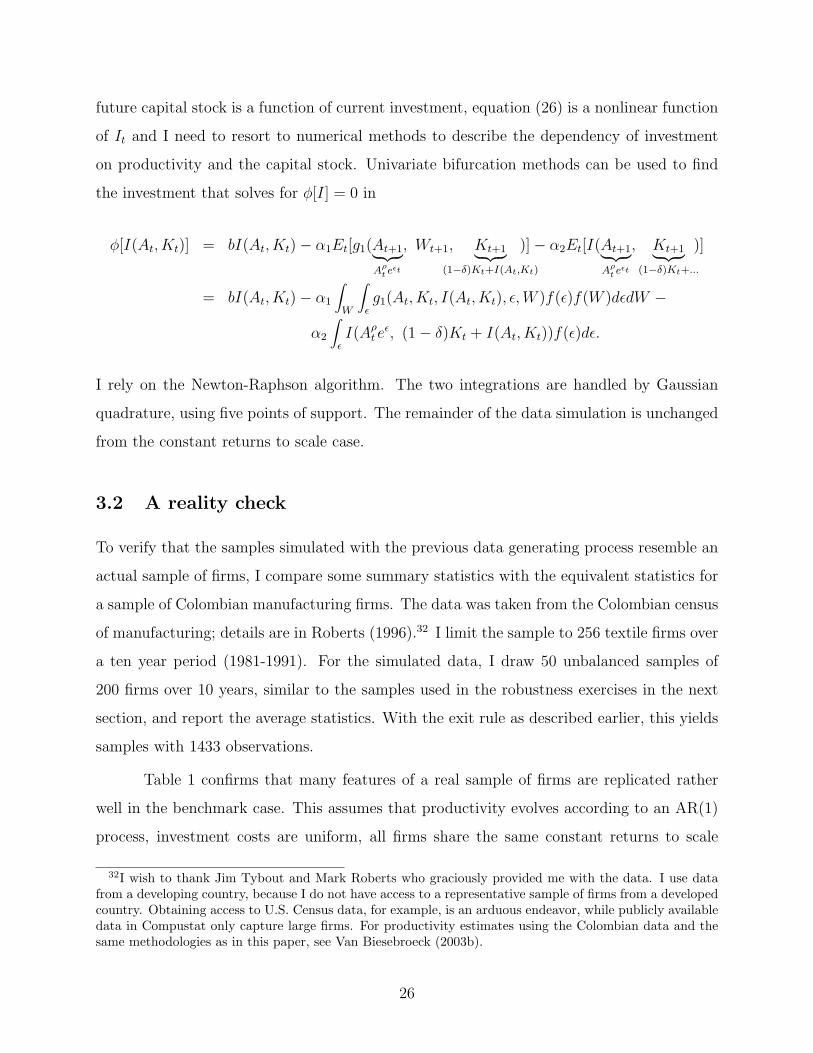
future capital stock is a function of current investment, equation (26) is a nonlinear function

of It and I need to resort to numerical methods to describe the dependency of investment

on productivity and the capital stock. Univariate bifurcation methods can be used to find

the investment that solves for φ[I] = 0 in

φ[I(At, Kt)] = bI(At, Kt)− α1Et[g1(At+1︸ ︷︷ ︸Aρ

t eεt

, Wt+1, Kt+1︸ ︷︷ ︸(1−δ)Kt+I(At,Kt)

)]− α2Et[I(At+1︸ ︷︷ ︸Aρ

t eεt

, Kt+1︸ ︷︷ ︸(1−δ)Kt+...

)]

= bI(At, Kt)− α1

∫W

∫εg1(At, Kt, I(At, Kt), ε,W )f(ε)f(W )dεdW −

α2

∫εI(Aρ

t eε, (1− δ)Kt + I(At, Kt))f(ε)dε.

I rely on the Newton-Raphson algorithm. The two integrations are handled by Gaussian

quadrature, using five points of support. The remainder of the data simulation is unchanged

from the constant returns to scale case.

3.2 A reality check

To verify that the samples simulated with the previous data generating process resemble an

actual sample of firms, I compare some summary statistics with the equivalent statistics for

a sample of Colombian manufacturing firms. The data was taken from the Colombian census

of manufacturing; details are in Roberts (1996).32 I limit the sample to 256 textile firms over

a ten year period (1981-1991). For the simulated data, I draw 50 unbalanced samples of

200 firms over 10 years, similar to the samples used in the robustness exercises in the next

section, and report the average statistics. With the exit rule as described earlier, this yields

samples with 1433 observations.

Table 1 confirms that many features of a real sample of firms are replicated rather

well in the benchmark case. This assumes that productivity evolves according to an AR(1)

process, investment costs are uniform, all firms share the same constant returns to scale

32I wish to thank Jim Tybout and Mark Roberts who graciously provided me with the data. I use datafrom a developing country, because I do not have access to a representative sample of firms from a developedcountry. Obtaining access to U.S. Census data, for example, is an arduous endeavor, while publicly availabledata in Compustat only capture large firms. For productivity estimates using the Colombian data and thesame methodologies as in this paper, see Van Biesebroeck (2003b).

26

production technology, and a standard deviation of 0.5 for the measurement error is added

to all variables. The most important difference of the simulated versus the Colombian data

is the lower variation of investment and capital—but not the investment share in capital—

and the wage share. In the benchmark case, all heterogeneity between firms is introduced

through the wage rate, a fixed productivity term subject to i.i.d. shocks that decay rapidly,

and random measurement error. Adding heterogeneity in other parts of the model, in Section

4.4, provides a better fit with the real data. Heterogeneity in investment costs leads directly

to much higher standard deviations on investment and capital. Random coefficients in the

production technology makes the wage share statistics more similar to the Colombian ones,

almost by construction.33

Estimation of a Cobb-Douglas production function by OLS also produces similar

results for both samples. With the simulated data, the labor coefficient is overestimated

relative to its true value of 0.6, with a downward bias in the capital coefficient. This ten-

dency will show up in the majority of the exercises later on, even with more sophisticated

estimation methods. Returns to scale are erroneously estimated to be increasing. Enforcing

constant returns to scale (results not reported) brings the labor coefficient down, closer to

its true value. The exit of relatively less productive firms from the sample leads to a positive

coefficient on the time trend, even though αt is zero in the data generating process. In the

Colombian data, many of the same tendencies seem to be at work. The labor coefficient is

surprisingly high, especially relative to the modest 0.62 average wage share, while the capital

coefficient is implausibly low. Some of the 6.1% productivity growth in the Colombian case

is likely to be attributable to selection.

[Table 1]

Table 2 illustrates that the partial correlation coefficients between all observable vari-

ables for the simulated data match the corresponding correlations for the Colombian sample

reasonably well. Output has the highest correlations with the other variables, while invest-

ment has the lowest, both in the simulated (top-right) and actual (bottom-left) samples.

33A translog production function will also produce variation in the wage share, but the investment functioncannot be solved analytically in that case. Moreover, the added generality of flexible functional forms onlybecome really valuable if more than two inputs are included.

27

Correlations between output and inputs are large and positive and those with labor and

wages exceed that with capital.

For the results limited to a single year, to focus on the across firm correlation, the

similarity is at least as high. The correlation over time, in the bottom panel of Table 2, is

less well captured. Correlations between year-on-year growth rates of the different variables

are generally higher for the simulated data. The growth rates of output and investment

are especially more alike those of other variables. A likely reason is that the AR(1) process

dominates the fixed effect in modeling persistency of the unobserved productivity in the

benchmark case. Changes in variables, especially investment and output, will have a built-

in persistence over time as firms respond gradually to productivity shocks. Increasing the

variance of the fixed effect or lowering the autoregressive coefficient or the variance of the

productivity shocks, in Section 4.2, will lower the correlation of the growth rates in the

simulated samples.

[Table 2]

4 Simulation Results

Using the simulated samples, productivity levels (TFPit = logAit− logAt) and growth rates

(TFPGit = logAit − logAit−1) are estimated using all the previously discussed methodolo-

gies. As a benchmark, productivity measures are also calculated using least squares estimates

of the production function parameters in equation (10). The table below summarizes the

superscripts and links to formulas for the different estimation methods.

4.1 The benchmark model

In this section, the different methodologies are compared using data generated from the

benchmark model; the same that was used to compare the simulated with the Colombian

data in the previous section. All firms share the same investment function and production

technology. All variables are observed with measurement error of equal variance. Produc-

tivity is the sum of two terms, a normally distributed fixed-effect (with standard deviation

28

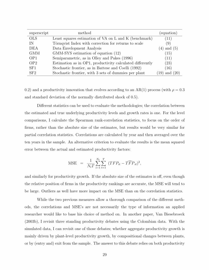
superscript method (equation)

OLS Least squares estimation of VA on L and K (benchmark) (11)IN Tornqvist Index with correction for returns to scale (9)DEA Data Envelopment Analysis (4) and (5)GMM GMM-SYS estimation of equation (12) (15)OP1 Semiparametric, as in Olley and Pakes (1996) (11)OP2 Estimation as in OP1, productivity calculated differently (23)SF1 Stochastic frontier, as in Battese and Coelli (1992) (16)SF2 Stochastic frontier, with 3 sets of dummies per plant (19) and (20)

0.2) and a productivity innovation that evolves according to an AR(1) process (with ρ = 0.3

and standard deviation of the normally distributed shock of 0.5).

Different statistics can be used to evaluate the methodologies; the correlation between

the estimated and true underlying productivity levels and growth rates is one. For the level

comparisons, I calculate the Spearman rank-correlation statistics, to focus on the order of

firms, rather than the absolute size of the estimates, but results would be very similar for

partial correlation statistics. Correlations are calculated by year and then averaged over the

ten years in the sample. An alternative criterion to evaluate the results is the mean squared

error between the actual and estimated productivity factors:

MSE =1

NtT

Nt∑i=1

T∑t=1

(TFPit − TFP it)2,

and similarly for productivity growth. If the absolute size of the estimates is off, even though

the relative position of firms in the productivity rankings are accurate, the MSE will tend to

be large. Outliers as well have more impact on the MSE than on the correlation statistics.

While the two previous measures allow a thorough comparison of the different meth-

ods, the correlations and MSE’s are not necessarily the type of information an applied

researcher would like to base his choice of method on. In another paper, Van Biesebroeck

(2003b), I revisit three standing productivity debates using the Colombian data. With the

simulated data, I can revisit one of those debates; whether aggregate productivity growth is

mainly driven by plant-level productivity growth, by compositional changes between plants,

or by (entry and) exit from the sample. The answer to this debate relies on both productivity

29

level and growth estimates. The decomposition results are in Table 4 and will be discussed

after the correlation and MSE results, for which the averages over fifty simulated samples

are in the first column of Table 3. The average input coefficient estimates, as well as the

sum of the MSE for each input coefficient, are also included.

In the benchmark case, the Olley-Pakes method estimates productivity levels most

accurately, especially if the random measurement error is taken out (OP2). The correla-

tion between estimated and true productivity is highest and the MSE is lowest. The least

restrictive stochastic frontier estimator (SF2), with three sets of dummies per firm, comes

in second. Using the correlation criterion, the two estimators are very close, 0.76 for OP2

versus 0.70 for SF2. The MSE criterion accentuates the difference. It is almost twice as large

for SF2. Both the index numbers and data envelopment results are still very respectable.

The performance of the DEA method is notably better for the correlation criterion than

using MSE, which is not surprising as the efficiency measures had to be converted to log

productivity differences. Only the GMM and the first stochastic frontier (SF1) estimators

barely leave the naive least squares estimator behind, producing a correlation with true

productivity just exceeding 0.30. The difference between the best and worse estimators are

definitely not negligible.

[Table 3]

The different estimators are less accurate and produce relatively similar results for

productivity growth. The Olley-Pakes estimator is still preferred, but the index number

calculations are almost equally accurate. Most other methods are not far behind, with

the exception of the second stochastic frontier method. SF2 yields results that are hardly

correlated with the true productivity growth rates. On the other hand, the MSE is second

lowest, indicating that the size of the growth rates was captured relatively well. It turns out

that methods that estimate productivity levels very accurately are not necessarily equally

adapt at estimating productivity growth, and vice versa, e.g. the index numbers.34

The bottom two panels in Table 3 contain the coefficient estimates that drive the

34The underlying DGP contains no built-in productivity growth, but in a sample of surviving firms averageproductivity growth is positive because of selection.

30

productivity results. The true labor coefficient is 0.6 throughout and returns to scale are

constant. The least squares results have the predicted bias: the labor coefficient is overes-

timated and the reverse is true for the capital coefficient. Returns to scale are estimated

to be increasing, in most cases significantly so. The GMM and SF1 results hardly improve

on the OLS results. The upward bias in the labor coefficient is only slightly reduced; the

capital coefficient is estimated even lower, which goes in the wrong direction. The OP and

SF2 estimators produce labor coefficient estimates that are notably lower, but the capital

coefficient is now hardly different from zero anymore. The labor and capital shares that

are used in the index numbers—obtained without estimation, but scaled down in the TFP

calculations according to (8) as returns to scale are estimated to be increasing—turn out to

be closest to the truth. The average input weights used in the DEA are also closer to the

true input shares than any of the parametric estimates.35

The results for the decomposition of aggregate productivity growth (from year one

to year ten) are in Table 4.36 One can aggregate individual firms using shares in an input

aggregate (LαLit K

αKit ), in the top panel, or using output shares, in the bottom panel. The

results are similar using both weights and I will only discuss the former. Aggregate produc-

tivity grew by 7.7% over ten years. The different methodologies produce a wide range of

estimates; the DEA, OP2 and OP1 methods come closest and the GMM and SF2 methods

are least accurate, at opposite extremes.

This aggregate growth is decomposed into the contribution of plants that survive over

ten years and those that exit from the sample. Less productive plants leaving the sample

adds 6.2% to aggregate productivity growth. This is almost the entire productivity advance,

not surprisingly, as there is no built-in productivity growth in the data generating process.

All methods get the sign right and the methods that predicted aggregate growth best, also

isolate the effect of exit most accurately: DEA, OP1 and OP2. Surviving plants contribute

only modestly to productivity growth. The SF2 results overestimate their contribution, while

the GMM estimator inexplicably finds a very strong negative effect.

35The MSE statistics for IN and DEA sum over the fifty samples, using the average input coefficients.While it is possible to use the observation-specific input shares and sum over 50×1433 observations, thiswould not be comparable to the parametric results.

36For the exact decomposition formula, I refer to Van Biesebroeck (2003b).

31

The contribution of surviving plants is further decomposed. Using initial input share

as weight on productivity growth for surviving plants reveals that, on average, productivity

growth at the plant-level was strongly negative, adding up to -21.7%. The range of estimates

is even more disparate and the DEA method, where plant-level growth rates are constructed

ad-hoc, is surprisingly the most accurate. Summing up changes in input shares, weighted

by initial productivity, indicates that less productive plants used an even larger share of

inputs by the end of the sample, lowering aggregate productivity by 21.1%. Similar to the

within component, the OLS and SF1 methods get it completely wrong. The GMM methods

is now most accurate, followed by DEA. The largest contribution to aggregate productivity

is made by co-movements in input shares and productivity. Plants improving productivity,

while at the same time increasing their input use, raise aggregate productivity by 44.4%.

For this to happen output growth has to outweigh input growth. OLS, GMM, and SF1 miss

this large positive effect completely and assign it a negative contribution. While a negative

correlation between input growth and productivity growth is intuitive, it is strongly at odds

with the data generating process. The DEA, SF2, and OP2 methods approach the actual

contribution most closely.

The GMM, SF1, and OLS methods predict an incorrect sign for many components

and estimate many magnitudes quite inaccurately. The OP1 and SF2 methods estimate

all signs correctly, but are not very successful in estimating the magnitudes of the different

contributions. The decomposition by the DEA and OP2 methods are clearly most reli-

able. Using output weights instead, these two methods tend to overestimate the different

contributions, but to a lesser extent than the other approaches.

[Table 4]

4.2 Different specifications for productivity

The results in subsequent columns of Table 3 are for variations in the specification of the

unobserved productivity term in the data generating process. The benchmark model in

column 1 contained three components that contributed to the persistency of productivity

over time, each of these is now studied in isolation. In the second column, only the AR(1) part

32

is maintained, while in the third column all productivity differences are constant over time.

In the fourth specification, the productivity shock is completely transitory, disappearing after

a single period. In each specification all variables are observed with the same measurement

error as before.

Looking across the different columns of Table 3, the results seem to be all over the

map. At the very least, this leads to one solid conclusion: no single method is the most

appropriate for every form of underlying productivity. No method has one of the three highest

correlations with true productivity in each of the four specification, not for productivity levels

nor for growth rates. At the same time, for each of the specifications considered, at least

one method manages to achieve a correlation of 0.73 or higher.

Still, the performance of different methods is not completely random. Overall, the

OP2 method has a high correlation for almost all specifications. It outperforms OP1 in most

cases, especially for productivity differences that are constant over time. The big exception

is the last column, where productivity is completely transitory. Here, OP1 is superior and

the difference is very large, as OP2 measures register hardly any positive correlation with

true productivity. Both methods rank at the top of the pack in most specifications, but the

inability of OP2 to pick up transitory shocks does not make either method clearly preferable

over the other.

The choice between the two stochastic frontier methods is more clear-cut. SF2, which

takes out the random measurement error, outperforms SF1 in productivity level estimations,

except for completely transitory productivity differences. The differences between the two in

the transitory case is much smaller than for the two Olley-Pakes variants, while the advantage

of SF2 is larger in the first three columns. SF2 is clearly preferable to estimate levels. For

productivity growth, on the other hand, the conclusion is reversed. Here, SF1 dominates SF2,

although neither ranks among the most attractive approaches. The surprising conclusion is

that SF2 is one of the best ways to estimate productivity levels, especially when there is

a fixed-effect, but it has the lowest correlation with productivity growth of all methods

considered.

The reverse is true for the index numbers. While lousy at estimating productiv-

ity levels, except when all productivity differences are transitory, they excel at estimating

33

productivity growth. Both findings are as expected. When there is no risk of confounding

random measurement error with structural productivity differences, they perform well. Their

widespread use in estimating productivity growth also seems justified.37 DEA is equally apt

at estimating productivity differences if they are completely transitory. Surprisingly, the

method seems relatively better at estimating growth rates than levels.

Finally, the OLS results are among the weakest of the bunch. There is some payoff

to more sophisticated approaches to estimate productivity. However, the payoff is marginal

or even negative for the GMM approach.

Looking across specifications, the nonparametric estimators, IN and DEA, have an

especially hard time coping with a permanent productivity component, where the stochastic

frontiers excel. The semiparametric estimators, OP1 and OP2, are best able to deal with

autoregressive components to productivity. If all productivity is transitory, methods that

take out random measurement error, OP2 and SF2, perform awfully, while the nonparametric

methods perform great. It is, of course, impossible to know how productivity evolves for

actual data, which makes the enormous differences between methods worrying. One could

prefer the index numbers to estimate productivity levels if differences are transitory, running

the risk of very inaccurate estimates if true productivity is relatively constant over time.

Similarly, a prior expectation of stable productivity differences might lead one to use OP2

or SF2, with the risk of missing the mark widely if real differences are transitory.

Glancing over the different coefficient estimates in the bottom panels, we find that the

upward bias in the labor coefficient depends negatively on the persistence of productivity over

time. If transitory shocks are important, the problem is especially pronounced. Even though

the correlation between productivity estimates is reasonably high, the input coefficients are

estimated surprisingly off-mark. The OLS estimator yields an average estimate for scale

economies ranging from 0.34 to 1.16 across specifications and most other estimators are not

much better. No standard errors are reported on these coefficient estimates, but they are

generally estimated very precisely. This is worrying as counterfactual simulations based on

37It is worth noting that two of the preferred estimators are generally not implemented as I did here.Studies using the semiparametric estimator have followed the original and used OP1. Studies calculatingproductivity as an index number generally force returns to scale to be constant.

34

the production function depend directly on the point estimates of the input coefficients.

In sum, I believe it is fair to conclude that the OP2 estimator performs best if pro-

ductivity is relatively persistent, with OP1 and SF2 also producing reliable estimates. In

the face of transitory productivity shocks, it is best abandon the parametric framework,

especially methods that attempt to take out measurement error, and stick with the index

numbers.

4.3 Varying the severity of measurement error

Next, I investigate the sensitivity to measurement error, assuming throughout that produc-

tivity evolves according to the benchmark specification, i.e. with an AR(1) component and

small fixed-effect. In all columns of Table 5, normally distributed measurement error with

equal variance is added to all observable variables. In successive columns, the standard de-

viation, σx in (29), is gradually increased from 0 to 1.25. For some methods, IN, DEA, and

SF2, this leads to a gradual decrease in the correlation between estimated and actual pro-

ductivity levels, but this trend is by no means universal. For the OP1 and OP2 estimators,

the correlations decrease gradually with a sudden but isolated and inexplicable improvement

for one standard error. For the OLS and SF1 methods, the pattern of the correlations for

increasing measurement error is U-shaped. More measurement error leads initially to lower

correlations, but this bottoms out in the benchmark case and correlations increase for larger

measurement errors. The SF1 method even performs best with very high measurement error.

Finally, for the GMM estimator, the correlations start out very low, increase initially, but

decrease eventually when measurement error grows very large. Everything seems possible.

It is comforting to find that the parametric methods perform best when measurement

error gets very large, especially OP2 and SF2, which explicitly take out additive measurement

error. Note the remarkable resilience of SF2, having only 0.1 lower correlation even for an

enormous amount of measurement error. On the other hand, it is surprising to find that

many parametric methods give poor results when there is no or very low measurement error.

The explication for this can be found in the bottom panels. The much stronger correlation

between labor input and productivity in the absence of any measurement error leads to

35

very high labor coefficient estimates. The correction for endogenous input choices tends

to overcorrect. For example, the GMM and OP methods estimate the capital coefficient

close to or even above its true value of 0.4 without a corresponding decrease in the labor

coefficient estimate relative to OLS. More measurement error lowers the coefficient estimates,

but unfortunately this affects the capital as much as the labor coefficient.

The haphazard evolution of correlations with productivity level stands in marked

contrast with the uniformity of experience for productivity growth calculations. Here, cor-

relations decrease monotonically, with as lone exception an isolated bump in correlation for

the GMM estimator for a standard error of 1.00. In every other case, more measurement

error translates into lower correlations and higher MSE. The rate of worsening is higher for

the productivity growth calculations than for levels, which makes sense as the measurement

error is i.i.d. and two time periods are involved in the growth calculations.

Even though the pattern is homogeneous, the methods are affected to a different

extent. The OP methods are affected most, dropping from the top two spots to number

three and seven. While they achieve an astounding correlation of 0.95 and 0.89 without

measurement error, these fall by at least three quarters when the errors get very large. It is

surprising to find that the OP2 method, which is supposed to take out measurement error, is

affected even more than OP1. At the other side of the spectrum, the SF2 method, which also

takes out measurement error, is hardly affected, not even for large errors, although it started

from a very low correlation. The robustness of this method is even more apparent using the

MSE criterion. It is noteworthy, as well, that the deterministic index number calculations

produce very robust productivity growth estimates. For small or moderate errors, only the

Olley-Pakes measures are preferred, while the index numbers have the highest correlations

with true productivity if measurement error gets very high. The SF1 and GMM methods

are also rather resilient in the face of measurement error. Their correlations drop for initial

increases in measurement error, but bottom out relatively fast.

[Table 5]

In the previous exercise, the size of measurement error was the same for all variables.

Given the considerable differences in standard error for the different variables in Table 1, this

36

is admittedly unrealistic. In Table 6, the benchmark comparison is repeated in column 1;

results for a standard deviation equal to one third of the standard deviation of the variables

in the Colombian data set are in column 2; measurement error with a standard deviation

of one third of the average standard deviation of the simulated variables without standard

error is added to each variable in column 3.

Most findings are robust to the assumption of uniform or varying size of measurement

error. In the productivity level calculations, the index method is most affected and the SF2

method least. The ranking of the different methods hardly depends on the assumption on

the relative size of measurement error added to different variables, even though it depended

crucially on the absolute size of measurement error in Table 4. For productivity growth, the

results for the OP1 and SF2 methods hardly change, while the index numbers are again most

affected. The index numbers are especially hard-hit when the error is proportional to the

variation in the underlying variable without measurement error, not surprising given that

the wage bill is one of the most volatile variables.

With measurement error proportional to the standard deviation of the underlying

variables, arguably the most natural assumption, the average correlation both for produc-

tivity levels and growth rates is reduced relative to the benchmark case with uniform errors.

The SF2 measures have the highest correlation with unobserved productivity levels and OP1

edges past OP2 for productivity growth estimates. Using the MSE criterion, the method of

choice would unambiguously be the OP2 method. The index numbers lose much of their ap-

peal. The disparity in correlations comparing across methods remains virtually unchanged.

[Table 6]

Finally, Table 7 shows the impact of measurement error when only a single variable

is measured imprecisely. All variables but one are measured with tiny measurement error

(σx = 0.1), while each variable in turn is observed with a lot of noise, adding measurement

error with a standard deviation of 0.75.

Adding noise to output, in column 2, cuts the level correlations approximately in

half relative to the low measurement error case, in column 1. This masks large differences.

The OP2 estimator is not affected in the least; it even increases its correlation with true

37

productivity. All other parametric estimators turn out to be particularly vulnerable. Only

the deterministic approaches, IN and DEA, post correlations that are at least half the cor-

relations in the low measurement error case. Results for productivity growth are almost

identical. The only parametric method that holds its ground is OP2, while the deterministic

approaches become relatively more attractive. The correction for measurement error in the

semiparametric methodology works remarkably well. The coefficient estimates of the OP

estimator are by no means better than for the other methods, which is also reflected in the

poor performance of OP1.

When the capital stock is the most mismeasured variable, results are very different.

Most methods are much less affected, not surprisingly given that the capital coefficient

is relatively small and estimated even smaller. More surprisingly, the Olley-Pakes results

improve substantially and the GMM method improves enormously. Both estimators rely

on lags for the identification of the capital parameter. The capital coefficient is estimated

near zero for all methods, but this tends to be less damaging for productivity estimates

than the overestimation of returns to scale, which is ubiquitous with low measurement error.

Productivity growth estimates only suffer noticeably from imprecisely observed capital if one

uses the OLS or SF1 methodology. In a sense, these results are reassuring, as capital is often

the variable most suspect to be measured with error.

All parametric methods estimate productivity levels and growth rates more accurately

if labor is measured with error. It tends to reduce the positive bias in the labor coefficient

estimate. Only the index numbers are extremely sensitive to imprecisely measured labor

input. Measurement error in the wage bill only affects the index number calculations, but

here it tends to raise the correlations slightly. It lowers the wage share in output, but given

that the estimated returns to scale are unaffected (estimated by OLS), it increases the capital

share. The net effect is to lower the MSE of the coefficient estimates, which in turn leads to

lower MSE and higher correlations for productivity level and growth.

Obviously, measurement error in investment only affects the Olley-Pakes results. The

impact is relatively large, lowering the level and growth correlations by a third for OP1 and

by more than half for OP2. Given that investment is more likely to be measured with error

than output, labor, or wages, this finding should not be discarded too easily.

38

[Table 7]

4.4 Allowing for plant heterogeneity

Thus far, the data generating process was identical for all firms, assuming the same produc-

tion technology and investment cost function. The only structural sources of variation were

the random wages and productivity shocks. Adding random measurement error, we were

able to match most of the volatility and correlation between observed variables with the

corresponding statistics of a real-world sample of firms. Heterogeneity across plants provides

an alternative to measurement error to make the simulated samples resemble actual data.

Several possibilities are explored.38

The first column in Table 8 repeats the benchmark results as comparison. In subse-

quent columns, more structural heterogeneity is introduced and the measurement errors are

omitted. The statistics in the second column are generated from a sample of plants that differ

in the adjustment cost of investment, the b coefficient in g(I); heterogeneity that is persis-

tent over time. The third column introduces transitory firm heterogeneity in the investment

function instead. The cost of new capital is assumed to be i.i.d. distributed across firms

and over time, just like wages. The last three columns introduce heterogeneous production

functions, always persistent over time. In column 4, the labor coefficient varies with opposite

variation in the capital coefficient, keeping returns to scale constant. In column 5, on the

other hand, returns to scale vary freely, but the relative importance of labor and capital is

as before, 60% and 40%. Finally, in column 6, both input coefficients vary independently

across firms, leading to variable scale economies as well. In the latter two cases, I have to

resort to numerical solutions for the investment equation.

Most methods, even the Olley-Pakes estimators, deal well with heterogeneous invest-

ment costs. The correlations are almost uniformly higher than in the benchmark case for

homogeneous firms, for productivity levels as well as for growth rates. Often, they even

exceed the correlations in the no measurement error case, column 1 in Table 5. Persistent

38E.g. adding a transitory shock to the price of capital in the investment cost function brings the standarddeviations of capital and investment much closer to the values for the Colombian data in Table 1.

39

heterogeneity is handled better than transitory. For productivity growth and transitory dif-

ferences, the Olley-Pakes methods are affected most, even though they remain among the

most accurate ones. The coefficient estimates indicate that the higher estimate for the labor

coefficient is the main culprit. For an investment function with random variation across

firms that the method cannot pick up, the endogeneity adjustment does not work nearly as

well.

Heterogeneity in the labor coefficient improves the results for some and worsens them

for other methods, but most importantly, it reduced the differences.39 No method achieves

a Spearman rank correlation coefficient over 0.68, while the worst method still achieves a

correlation of 0.32. Excluding the stochastic frontier methods, which end up at the bottom

of the pack, all methods become virtually indistinguishable to estimate productivity levels

and only the index numbers have a less than 0.7 correlation for productivity growth. For

productivity growth, all correlations coefficients increase considerably, relative to the bench-

mark case where measurement error generated the variation. Surprisingly, the index number

is one of the most affected estimators, even though homogeneity in the technology is not even

assumed. Some of the deterioration is driven by the overestimate of average scale economies

by OLS. Enforcing constant returns to scale would certainly improve the estimates as 64%

of the weight is on labor, in line with previous results.

All methods, save for GMM, perform worse if returns to scale vary freely across plants.

The average correlation for productivity levels drops from 0.51 to 0.37. The GMM estimator

manages to estimate the capital coefficient accurately, with a lower labor coefficient than in

most specifications. Its improved correlation is even more apparent for productivity growth.

The results are similar whether the relative importance of both inputs are left free or not.

The nonparametric approaches, IN and DEA, are affected most in each of the last three

columns. This is unexpected as both estimators do not assume plants to be homogeneous

and we expected them to shine in this exercise. It severely lowers their attractiveness as

dealing with unobserved heterogeneity in the primitives should be their advantage. On the

other hand, these nonparametric methods were affected less by measurement error than most

parametric approaches, which is also counterintuitive.

39The actual input coefficients in the bottom panel of Table 7 are the averages across plants.

40

[Table 8]

The results in Table 8 indicate that all methods have less problems with structural

sources of heterogeneity than with random measurement error. If we believe that most of the

variation in the data are random errors, there is little hope of estimating productivity well.

Deterministic methods were not even found to be disadvantaged in dealing with measurement

error. On the other hand, if the variation is driven by firms facing different factor prices,

investment functions, or production technologies, the prospects are better. It hardly matters

whether the methods explicitly allow for the heterogeneity or not. Most parametric methods

are not particularly affected by random variation in the production function parameters and

the semiparametric method deals adequately with different investment equations.

4.5 Varying returns to scale

The last robustness check on the estimation methodologies is to vary the scale economies

of the data generating process, keeping them the same for all plants, and to estimate pro-

ductivity with constant returns enforced or not.40 In the odd columns of Table 9 returns to

scale are estimated freely, while the actual scale economies for the underlying data gener-

ating process are, respectively, decreasing, constant, and increasing. In the even columns,

constant returns to scale is enforced on the estimator, while the same three data generating

processes are considered. For the Olley-Pakes methodology, constant returns are enforced

by only estimating the first stage. For the other parametric methodologies, the production

function is estimated by regressing the logarithm of output per worker on the logarithm of

the capital-labor ratio. In each case, the capital coefficient is calculated as one minus the

estimated labor coefficient.

The most important finding in Table 9 is that, with the exception of SF2, the cor-

relations for the productivity level are higher when constant returns to scale are enforced;

40Ideally, I would like to investigate the impact of the functional form of the production function morethoroughly, as was done with U.S. data in Berndt and Khaled (1979). Previous Monte Carlo studies, forexample Gagne and Ouellette (1998) and sources cited there, use exogenously generated inputs. In thecurrent framework, input choices consistent with the firm’s optimization problem could not even be solvedexplicitly for the simplest of technologies (Cobb-Douglas) if scale economies are present. Incorporating moreflexible functional forms is left for future research.

41

irrespective of the data generating technology. Restricting returns to scale to unity is gen-

erally a good idea, independent of the actual scale economies. For some methods, e.g. the

Olley-Pakes and GMM estimators, the differences are quite large.

The estimated returns to scale are fairly independent of the data generating process

for all parametric methods. The labor coefficient is estimated only slightly higher if the data

is generated with larger scale economies, while the capital coefficient estimate even goes

down for some methods. While returns to scale are invariably overestimated if they are truly

decreasing, the estimates are much closer to the truth for increasing scale economies. The

average correlations for productivity levels are higher for higher underlying scale economies.

For productivity growth, the SF2 results are still more accurate if constant returns

are not enforced (even when they are really constant), but the same is now also true for

OLS, GMM, and SF1. Even when returns to scale are constant it is best not to enforce

this. Each of these methods estimate the capital coefficients extremely small, often even

negative.41 However, the IN and OP2 methods still show a marked increase in correlation if

returns to scale are fixed. As these are the two methods that have the highest correlations

and are probably most attractive to estimate productivity growth, allowing variable returns

to scale does not seem necessary.

Not a single method finds it optimal to allow for variable returns if the underlying

data is generated by a nonconstant returns to scale technology, and vice versa; fixing constant

returns to scale only when it is correct for the simulated data. The correlations, both for

productivity levels and growth, are relatively independent of the returns to scale in the data

generating process. They are more dependent on the scale assumptions used in estimation.

[Table 9]

41The measurement error added to all variables for the exercises in Table 9 has a standard deviation ofonly 0.1. In light of the results in Table 5, the results for the parametric methods might look differently iflarger measurement error were incorporated.

42

5 Lessons

I believe a number of findings from these exercises were unexpected:

• It does matter what method is used to estimate productivity. For different assumptions

on the evolution of productivity, an inherently unobservable phenomenon, different

methodologies are preferred.

• The Olley-Pakes estimator is remarkably robust to a number of complications. The

OP2 estimator performs especially well when a large part of productivity is nontransi-

tory.

• Most parametric methods are not very sensitive to small amounts of measurement

error, but do not perform well if errors get large. Moreover, some random noise helps

them to avoid overcorrecting for the biases in the production coefficient estimates. The

deterministic methods, DEA and IN, do not seem at a disadvantage in dealing with

random measurement error.

• The same two nonparametric methods, DEA and IN, that do not assume homogeneity

across firms, are not more robust than parametric methods in coping with heterogeneity

in adjustment costs or production technology.

• Using the same returns to scale assumption in estimation as the one used to generate

the data (constant or not), is necessary nor sufficient for accurate results.

43

References

Aigner, D., C. K. Lovell, and P. Schmidt (1977). Formulation and Estimation of StochasticFrontier Production function Models. Journal of Econometrics 6, 21–37.

Battese, G. E. and T. J. Coelli (1992). Frontier Production Functions, Technical Efficiencyand Panel Data: With Application to Paddy Farmers in India. Journal of ProductivityAnalysis 3, 153–69.

Berndt, E. R. and M. S. Khaled (1979). Parametric Productivity Measurement and Choiceamong Flexible Functional Forms. Journal of Political Economy 87 (6), 1220–45.

Blundell, R. W. and S. R. Bond (1998). Initial Conditions and Moment Restrictions inDynamic Panel Data Models. Journal of Econometrics 87, 115–43.

Blundell, R. W. and S. R. Bond (2000). GMM Estimation with Persistent Panel Data:An Application to Production Functions. Econometric Reviews 19 (3), 321–340.

Caves, D. W., L. R. Christensen, and E. W. Diewert (1982a). The Economic Theory ofIndex Numbers and the Measurement of Input, Output, and Productivity. Economet-rica 50 (6), 1393–1414.

Caves, D. W., L. R. Christensen, and E. W. Diewert (1982b). Multilateral Comparisonsof Output, Input, and Productivity using Superlative Index Numbers. Economic Jour-nal 92, 73–86.

Charnes, A., W. W. Cooper, and E. Rhodes (1978). Measuring the Efficiency of DecisionMaking Units. European Journal of Operational Research 2, 429–444.

Cornwell, C., P. Schmidt, and R. C. Sickles (1990). Productivity Frontiers with Cross-sectional and Time Series Variation in Efficiency Levels. Journal of Econometrics 46,185–200.

Diewert, W. E. (1976). Exact and Superlative Index Numbers. Journal of Econometrics 4,115–145.

Ericson, R. and A. Pakes (1995, January). Markov Perfect Industry Dynamics: A Frame-work for Empirical Work. Review of Economic Studies 62 (1), 53–85.

Farrell, M. J. (1957). The Measurement of Productive Efficiency. Journal of the RoyalStatistical Society, Series A. 120, 253–290.

Gagne, R. and P. Ouellette (1998, January). On the Choice of Functional Forms: Summaryof a Monte Carlo Experiment. Journal of Business and Economic Statistics 16 (1),118–124.

Griliches, Z. and J. A. Hausman (1986, February). Errors in Variables in Panel Data.Journal of Econometrics 31 (1), 93–118.

Griliches, Z. and J. Mairesse (1998). Production Functions: The Search for Identification.In S. Strom (Ed.), Econometrics and Economic Theory in the Twentieth Century: TheRagnar Frisch Centennial Symposium, pp. 169–203. Cambridge University Press.

Huang, C. J. and J.-T. Liu (1994, June). Estimation of a Non-neutral Stochastic FrontierProduction Function. Journal of Productivity Analysis 5 (2), 171–80.

44

Levinsohn, J. and A. Petrin (2003, April). Estimating Production Functions Using Inputsto Control for Unobservables. Review of Economic Studies 70 (2), 317–342.

Mairesse, J. and Z. Griliches (1990). Heterogeneity in Panel Data: Are There StableProduction Functions. In P. C. et al. (Ed.), Essays in Honor of Edmond Malinvaud,Volume 3, pp. 125–147. Cambridge: MIT Press.

Marschak, J. and W. H. Andrews (1944). Random Simultaneous Equations and the Theoryof Production. Econometrica 12, 143–205.

Meeusen, W. and J. van den Broeck (1977). Efficiency Estimation from Cobb-DouglasProduction functions with Composed Error. International Economic Review 8, 435–44.

Olley, G. S. and A. Pakes (1996). “The Dynamics of Productivity in the Telecommunica-tions Equipment Industry”. Econometrica 64 (6), 1263–97.

Roberts, M. (1996). Colombia, 1977-85: Producer Turnover, Margins, and Trade Ex-posure. In M. Roberts and J. R. Tybout (Eds.), Industrial Evolution in DevelopingCountries, Chapter 10, pp. 227–59. New York: Oxford University Press for the WorldBank.

Schmidt, P. and R. C. Sickles (1984). Productivity Frontiers and Panel Data. Journal ofBusiness and Economic Statistics 2, 367–374.

Seiford, L. L. and R. M. Thrall (1990). Recent Developments in DEA. The MathematicalProgramming Approach to Frontier Analysis. Journal of Econometrics 46, 7–38.

Solow, R. M. (1957). Technical Change and the Aggregate Production Function. Reviewof Economics and Statistics 39, 312–320.

Stevenson, R. E. (1980). Likelihood Functions for Generalized Stochastic Frontier Estima-tion. Journal of Econometrics 13, 57–66.

Stigler, G. J. (1976, March). Xistence of X-efficiency. American Economic Review 66 (1),213–16.

Syverson, C. W. (2001). Market Structure and Productivity. Ph.D. dissertation, Universityof Maryland.

Van Biesebroeck, J. (2003a, January). Productivity Dynamics with Technology Choice:An Application to Automobile Assembly. Review of Economic Studies 70 (1), 167–198.

Van Biesebroeck, J. (2003b, November). Revisiting some Productivity Debates. NBERWorking paper, No. 10065.

45

Table 1: Summary statistics for Colombian and simulated samples

Colombian sample Simulated samples1

(textile industry) (average over 50 samples)

Observed variables mean st.d. mean st.d.

log Y 7.49 1.36 7.56 1.90log K 5.29 1.73 3.92 0.93log L 3.91 1.04 4.29 1.78log WL 6.88 1.30 7.33 1.89log I 3.76 1.93 3.03 0.97

wage share 0.62 1.39 0.62 0.23investment share (if positive) 0.32 1.22 0.56 1.20

OLS regressionwith log Y as dependent variable2 mean s.e. mean s.e.log K 0.124 0.009 0.299 0.028log L 0.983 0.016 0.885 0.014time 0.074 0.004 0.019 0.007

R2 0.82 0.83number of firms 256 200number of observations (plant-years) 2164 20001 Parameters in the data generating process are set to their benchmark values, see Section 4.1.2 In the data generating process: aK=0.4, aL=0.6, and at=0.

46

Table 2: Correlation coefficients between all observed variables: Simulated & Colombia

All observations in levels:

log Y log L log WL log K log I

log Y 0.92 0.93 0.72 0.79log L 0.89 0.92 0.70 0.75 Simulatedlog WL 0.92 0.96 0.72 0.78 samplelog K 0.69 0.69 0.68 0.63 (10 years) log I 0.57 0.55 0.56 0.79

Colombian sample (1981-91)

Last year in levels:

log Y log L log WL log K log I

log Y 0.91 0.91 0.68 0.67log L 0.80 0.89 0.61 0.62 Simulatedlog WL 0.85 0.98 0.67 0.65 samplelog K 0.66 0.63 0.63 0.55 (year 10) log I 0.51 0.53 0.53 0.81

Colombian sample (1991)

Last year growth rates:

log Yt/Yt-1 log Lt/Lt-1 log WLt/WLt-1 log Kt/Kt-1 log It/It-1

log Yt/Yt-1 0.75 0.73 0.04 0.36log Lt/Lt-1 0.12 0.72 0.09 0.29 Simulatedlog WLt/WLt-1 0.18 0.94 0.05 0.30 samplelog Kt/Kt-1 0.20 0.07 0.07 -0.07 (year 9 to 10)log It/It-1 -0.12 0.07 0.09 0.54

Colombian sample (1990 to 1991)

47

Table 3: Different specifications for productivityAR coeff. (?) 0.3 0.5 0.0 0.0st. dev. of ? it 0.5 0.5 0.0 0.8st. dev. of ? i 0.2 0.0 0.2 0.0Productivity level: Spearman rank-correlation with true valuesOLS 0.308 0.373 0.329 0.313IN 0.547 0.595 0.211 0.764DEA 0.484 0.490 0.278 0.465GMM 0.357 0.395 0.225 0.254OP1 0.607 0.622 0.433 0.313OP2 0.762 0.825 0.631 0.022SF1 0.323 0.378 0.444 0.312SF2 0.703 0.559 0.728 0.187Productivity level: Mean squared errorOLS 0.652 0.550 0.348 0.821IN 0.500 0.418 0.392 0.416DEA 0.578 0.516 0.418 0.708GMM 0.569 0.551 0.375 0.907OP1 0.460 0.389 0.340 0.822OP2 0.181 0.096 0.033 0.624SF1 0.639 0.545 0.340 0.822SF2 0.314 0.268 0.170 0.687Productivity growth: correlation with true valuesOLS 0.300 0.325 0.000 0.314IN 0.401 0.490 0.000 0.767DEA 0.345 0.388 0.000 0.467GMM 0.287 0.314 0.000 0.254OP1 0.398 0.481 0.000 0.314OP2 0.467 0.733 0.000 0.022SF1 0.303 0.327 0.000 0.313SF2 0.102 0.136 0.000 0.046Productivity growth: Mean squared errorOLS 0.993 1.005 0.670 1.645IN 0.884 0.848 0.782 0.902DEA 0.948 0.961 0.800 1.398GMM 0.974 1.020 0.751 1.823OP1 0.798 0.766 0.620 1.647OP2 0.204 0.156 0.044 1.235SF1 0.983 1.001 0.614 1.647SF2 0.309 0.386 0.052 1.299Average coefficient estimatesactual 0.600 0.400 0.600 0.400 0.600 0.400 0.600 0.400OLS 0.861 0.297 0.877 0.204 0.467 0.320 0.975 0.002IN 0.714 0.444 0.654 0.452 0.494 0.297 0.618 0.408DEA 0.691 0.312GMM 0.859 0.221 0.885 0.129 0.514 0.478 1.007 -0.020OP 0.725 0.151 0.675 0.208 0.434 0.142 0.975 0.013SF1 0.857 0.287 0.875 0.199 0.399 0.152 0.976 0.003SF2 0.671 0.003 0.743 0.073 0.320 0.008 0.973 -0.004Coefficient mean square errorsOLS 0.081 0.116 0.027 0.302IN 0.010 0.003 0.050 0.002DEA 0.041GMM 0.119 0.117 0.029 0.359OP 0.080 0.044 0.096 0.295SF1 0.081 0.117 0.105 0.301SF2 0.165 0.129 0.234 0.306

48

Table 4: Decomposing aggregate productivity growth

Aggregate input weight aggregateexiting plants

surviving plants

within between correlation

actual 0.077 0.062 0.016 -0.217 -0.211 0.444OLS 0.021 0.009 0.012 0.091 0.177 -0.256DEA 0.088 0.057 0.031 -0.138 -0.122 0.291GMM -0.805 0.008 -0.812 -0.557 -0.240 -0.015OP1 0.104 0.059 0.046 -0.059 -0.031 0.136OP2 0.078 0.052 0.027 -0.091 -0.098 0.216SF1 0.027 0.011 0.016 0.082 0.169 -0.235SF2 0.190 0.110 0.080 -0.078 -0.098 0.256

Output weights aggregateexiting plants

surviving plants

within between correlation

actual 0.060 0.027 0.033 -0.167 -0.154 0.354OLS 0.111 0.025 0.086 -0.497 -0.448 1.031DEA 0.165 0.039 0.127 -0.333 -0.326 0.786GMM -0.904 0.005 -0.909 -1.370 -0.995 1.456OP1 0.033 0.002 0.031 -0.349 -0.275 0.655OP2 0.079 0.030 0.049 -0.371 -0.319 0.739SF1 0.031 0.006 0.024 -0.367 -0.293 0.684SF2 0.092 0.028 0.063 -0.565 -0.539 1.167

49

Table 5: Amount of measurement error(s x=0.00)

no error

(s x=0.10)

tiny error

(s x=0.25)

low error

(s x=0.50)

benchmark

(s x=0.75)

med-high error

(s x=1.00)

high error

(s x=1.25)

huge errorProductivity level: Spearman rank-correlation with true valuesOLS 0.434 0.403 0.335 0.308 0.324 0.348 0.367IN 0.930 0.844 0.673 0.547 0.488 0.445 0.407DEA 0.758 0.708 0.591 0.484 0.433 0.407 0.385GMM 0.095 0.145 0.256 0.357 0.390 0.482 0.380OP1 0.699 0.679 0.761 0.607 0.514 0.471 0.450OP2 0.653 0.662 0.819 0.762 0.662 0.572 0.496SF1 0.435 0.404 0.337 0.323 0.379 0.449 0.481SF2 0.777 0.760 0.719 0.703 0.700 0.691 0.675Productivity level: Mean squared errorOLS 0.310 0.324 0.395 0.652 1.067 1.623 2.307IN 0.132 0.158 0.240 0.500 0.954 1.622 2.528DEA 0.206 0.218 0.291 0.578 1.074 1.739 2.544GMM 0.411 0.414 0.407 0.569 0.949 1.400 2.263OP1 0.224 0.228 0.201 0.460 0.902 1.487 2.198OP2 0.244 0.239 0.157 0.181 0.229 0.276 0.319SF1 0.310 0.323 0.394 0.639 1.006 1.508 2.169SF2 0.188 0.190 0.203 0.314 0.590 0.957 1.352Productivity growth: correlation with true valuesOLS 0.609 0.550 0.413 0.300 0.256 0.235 0.224IN 0.844 0.713 0.516 0.401 0.353 0.319 0.290DEA 0.624 0.570 0.450 0.345 0.291 0.260 0.234GMM 0.615 0.522 0.378 0.287 0.254 0.301 0.234OP1 0.946 0.866 0.618 0.398 0.313 0.272 0.247OP2 0.892 0.856 0.741 0.467 0.320 0.240 0.190SF1 0.607 0.548 0.413 0.303 0.271 0.270 0.267SF2 0.140 0.128 0.108 0.102 0.102 0.099 0.093Productivity growth: Mean squared errorOLS 0.158 0.190 0.367 0.993 1.948 3.134 4.497IN 0.076 0.123 0.306 0.884 1.832 3.188 5.005DEA 0.153 0.183 0.347 0.948 1.939 3.248 4.802GMM 0.159 0.209 0.393 0.974 1.858 2.720 4.486OP1 0.026 0.066 0.236 0.798 1.676 2.808 4.150OP2 0.050 0.067 0.115 0.204 0.288 0.368 0.439SF1 0.158 0.191 0.367 0.983 1.865 2.870 4.017SF2 0.242 0.245 0.260 0.309 0.383 0.477 0.590Average coefficient estimatesactual 0.600 0.400 0.600 0.400 0.600 0.400 0.600 0.400 0.600 0.400 0.600 0.400 0.600 0.400OLS 0.965 0.228 0.958 0.237 0.929 0.268 0.861 0.297 0.782 0.291 0.698 0.269 0.614 0.242IN 0.844 0.349 0.851 0.343 0.824 0.373 0.714 0.444 0.599 0.474 0.497 0.472 0.410 0.449GMM 0.964 0.401 0.974 0.352 0.950 0.271 0.859 0.221 0.760 0.216 0.679 0.222 0.619 0.228OP 0.724 0.678 0.734 0.613 0.749 0.199 0.725 0.151 0.673 0.157 0.612 0.154 0.548 0.142SF1 0.966 0.225 0.959 0.235 0.929 0.265 0.857 0.287 0.752 0.257 0.618 0.205 0.500 0.160SF2 0.928 -0.083 0.914 -0.068 0.847 -0.027 0.671 0.003 0.498 0.008 0.366 0.008 0.273 0.006Coefficient mean square errorsOLS 0.163 0.155 0.127 0.081 0.047 0.029 0.028IN 0.024 0.026 0.020 0.010 0.007 0.017 0.049GMM 0.147 0.157 0.155 0.119 0.083 0.056 0.052OP 0.093 0.080 0.091 0.080 0.067 0.063 0.072SF1 0.165 0.156 0.128 0.081 0.046 0.042 0.071SF2 0.342 0.319 0.245 0.165 0.167 0.211 0.264

50

Table 6: Absolute or relative measurement error

(s x=0.50) benchmark (s x = 1/3 of real SD) (s x = 1/3 of no-error SD)

Productivity level: Spearman rank-correlation with true valuesOLS 0.308 0.270 0.305IN 0.547 0.648 0.381DEA 0.484 0.490 0.465GMM 0.357 0.323 0.284OP1 0.607 0.590 0.471OP2 0.762 0.787 0.623SF1 0.323 0.280 0.308SF2 0.703 0.673 0.691Productivity level: Mean squared errorOLS 0.652 0.572 0.765IN 0.500 0.385 0.747DEA 0.578 0.473 0.720GMM 0.569 0.500 0.777OP1 0.460 0.381 0.636OP2 0.181 0.177 0.243SF1 0.639 0.564 0.762SF2 0.314 0.256 0.392Productivity growth: correlation with true valuesOLS 0.300 0.264 0.367IN 0.401 0.492 0.272DEA 0.345 0.348 0.335GMM 0.287 0.258 0.336OP1 0.398 0.380 0.416OP2 0.467 0.528 0.411SF1 0.303 0.266 0.366SF2 0.102 0.091 0.098Productivity growth: Mean squared errorOLS 0.993 0.786 1.184IN 0.884 0.661 1.340DEA 0.948 0.723 1.232GMM 0.974 0.778 1.219OP1 0.798 0.631 1.081OP2 0.204 0.178 0.217SF1 0.983 0.781 1.183SF2 0.309 0.290 0.336Average coefficient estimatesactual 0.600 0.400 0.600 0.400 0.600 0.400OLS 0.861 0.297 0.946 0.174 0.742 0.578IN 0.714 0.444 0.654 0.468 0.824 0.498GMM 0.859 0.221 0.942 0.124 0.775 0.538OP 0.725 0.151 0.807 0.086 0.659 0.501SF1 0.857 0.287 0.943 0.170 0.742 0.573SF2 0.671 0.003 0.784 -0.005 0.620 0.015Coefficient mean square errorsOLS 0.081 0.172 0.055IN 0.010 0.007 0.030GMM 0.119 0.206 0.097OP 0.080 0.143 0.035SF1 0.081 0.172 0.054SF2 0.165 0.199 0.154

51

Table 7: Measurement error for different variables(s x=0.10) tiny

error

(s x = 0.10) (s y = 0.75)

(s x = 0.10) (s k = 0.75)

(s x = 0.10) (s l = 0.75)

(s x = 0.10) (sw = 0.75)

(s x = 0.10) (s i = 0.75)

Productivity level: Spearman rank-correlation with true valuesOLS 0.403 0.153 0.349 0.499 0.403 0.403IN 0.844 0.475 0.844 0.122 0.912 0.844DEA 0.708 0.384 0.686 0.598 0.708 0.708GMM 0.145 0.056 0.493 0.190 0.145 0.145OP1 0.679 0.327 0.934 0.836 0.679 0.462OP2 0.662 0.706 0.906 0.815 0.662 0.316SF1 0.404 0.154 0.371 0.499 0.404 0.404SF2 0.760 0.460 0.753 0.781 0.760 0.760Productivity level: Mean squared errorOLS 0.324 0.875 0.340 0.399 0.324 0.324IN 0.158 0.667 0.147 1.023 0.118 0.158DEA 0.218 0.765 0.226 0.419 0.218 0.218GMM 0.414 1.004 0.261 0.726 0.414 0.414OP1 0.228 0.761 0.103 0.544 0.228 0.306OP2 0.239 0.226 0.113 0.484 0.239 0.351SF1 0.323 0.874 0.332 0.398 0.323 0.323SF2 0.190 0.393 0.200 0.359 0.190 0.190Productivity growth: correlation with true valuesOLS 0.550 0.204 0.365 0.677 0.550 0.550IN 0.713 0.346 0.713 0.081 0.799 0.713DEA 0.570 0.264 0.538 0.469 0.570 0.570GMM 0.522 0.201 0.412 0.649 0.522 0.522OP1 0.866 0.368 0.846 0.832 0.866 0.612OP2 0.856 0.847 0.942 0.909 0.856 0.415SF1 0.548 0.204 0.372 0.675 0.548 0.548SF2 0.128 0.048 0.121 0.146 0.128 0.128Productivity growth: Mean squared errorOLS 0.190 1.297 0.269 0.429 0.190 0.190IN 0.123 1.203 0.141 1.673 0.097 0.123DEA 0.183 1.284 0.198 0.654 0.183 0.183GMM 0.209 1.332 0.254 0.550 0.209 0.164OP1 0.066 1.173 0.070 0.279 0.066 0.165OP2 0.067 0.073 0.053 0.099 0.067 0.211SF1 0.191 1.297 0.265 0.430 0.191 0.191SF2 0.245 0.343 0.245 0.287 0.245 0.245Average coefficient estimatesactual 0.600 0.400 0.600 0.400 0.600 0.400 0.600 0.400 0.600 0.400 0.600 0.400OLS 0.958 0.237 0.961 0.235 1.029 0.056 0.562 0.964 0.958 0.237 0.958 0.237IN 0.851 0.343 0.727 0.472 0.773 0.311 1.087 0.438 0.727 0.467 0.851 0.343GMM 0.974 0.352 0.986 0.331 1.010 0.038 0.588 1.274 0.974 0.352 0.974 0.351OP 0.734 0.613 0.734 0.545 0.740 -0.001 0.305 0.466 0.734 0.613 0.929 0.286SF1 0.959 0.235 0.960 0.234 1.026 0.053 0.564 0.959 0.959 0.235 0.959 0.235SF2 0.914 -0.068 0.920 -0.072 0.912 -0.007 0.495 0.073 0.914 -0.068 0.914 -0.068Coefficient mean square errorsOLS 0.155 0.162 0.303 0.321 0.155 0.155IN 0.026 0.014 0.022 0.063 0.014 0.026GMM 0.157 0.266 0.301 0.823 0.157 0.157OP 0.080 0.079 0.180 0.467 0.080 0.122SF1 0.156 0.162 0.302 0.315 0.156 0.156SF2 0.319 0.336 0.263 0.121 0.319 0.319

52

Table 8: Allowing for plant heterogeneity(s x=0.50)

benchmarkbi rit ßli & 1-ßli (ßl+ßk)i ßli & ßki

Productivity level: Spearman rank-correlation with true valuesOLS 0.308 0.442 0.443 0.523 0.221 0.306IN 0.547 0.970 0.966 0.554 0.409 0.418DEA 0.484 0.726 0.713 0.621 0.193 0.270GMM 0.357 0.558 0.358 0.602 0.497 0.494OP1 0.607 0.766 0.701 0.650 0.492 0.472OP2 0.762 0.746 0.651 0.681 0.573 0.599SF1 0.323 0.481 0.452 0.322 0.227 0.220SF2 0.703 0.757 0.763 0.402 0.345 0.295Productivity level: Mean squared errorOLS 0.652 0.312 0.311 0.298 0.430 0.415IN 0.500 0.098 0.105 0.394 0.467 0.615DEA 0.578 0.222 0.228 0.329 0.586 0.630GMM 0.569 0.240 0.315 0.256 0.278 0.365OP1 0.460 0.211 0.237 0.251 0.374 0.398OP2 0.181 0.244 0.285 0.238 0.320 0.320SF1 0.639 0.301 0.309 0.443 0.454 0.532SF2 0.314 0.188 0.196 0.436 0.466 0.569Productivity growth: correlation with true valuesOLS 0.300 0.497 0.539 0.902 0.839 0.878IN 0.401 0.928 0.922 0.556 0.482 0.496DEA 0.345 0.596 0.577 0.712 0.411 0.509GMM 0.287 0.508 0.538 0.869 0.883 0.888OP1 0.398 0.857 0.776 0.930 0.937 0.926OP2 0.467 0.945 0.626 0.879 0.877 0.869SF1 0.303 0.524 0.541 0.679 0.612 0.622SF2 0.102 0.148 0.126 0.140 0.135 0.140Productivity growth: Mean squared errorOLS 0.993 0.194 0.179 0.045 0.073 0.056IN 0.884 0.041 0.044 0.248 0.254 0.285DEA 0.948 0.166 0.174 0.137 0.281 0.247GMM 0.974 0.186 0.180 0.062 0.056 0.054OP1 0.798 0.068 0.098 0.034 0.044 0.042OP2 0.204 0.065 0.160 0.059 0.076 0.071SF1 0.983 0.184 0.178 0.132 0.155 0.150SF2 0.309 0.241 0.243 0.241 0.242 0.240Average coefficient estimatesactual 0.600 0.400 0.600 0.400 0.600 0.400 0.600 0.400 0.600 0.400 0.600 0.400OLS 0.861 0.297 0.999 0.107 0.981 0.129 0.781 0.579 0.842 0.568 0.792 0.635IN 0.714 0.444 0.780 0.325 0.786 0.324 0.882 0.479 0.938 0.473 0.914 0.515GMM 0.859 0.221 0.987 0.076 0.979 0.163 0.822 0.312 0.815 0.407 0.816 0.320OP 0.725 0.151 0.840 0.338 0.882 0.252 0.722 0.597 0.642 0.847 0.691 0.704SF1 0.857 0.287 0.989 0.116 0.981 0.127 0.933 0.195 0.960 0.186 0.955 0.168SF2 0.671 0.003 0.921 -0.153 0.931 -0.045 0.934 -0.070 0.934 -0.047 0.937 -0.034Coefficient mean square errorsOLS 0.081 0.245 0.219 0.071 0.089 0.100IN 0.010 0.020 0.020 0.036 0.043 0.045GMM 0.119 0.265 0.215 0.084 0.068 0.064OP 0.080 0.063 0.105 0.111 0.267 0.172SF1 0.081 0.233 0.220 0.154 0.176 0.182SF2 0.165 0.412 0.309 0.334 0.313 0.303

53

Table 9: Impact of specifiation errorsReturns to scale decreasing constant increasing

(aK+aL=0.8) (aK+aL=1) (aK+aL=1.2)

CRS enforced ? no yes no yes no yesProductivity level: Spearman rank-correlation with true valuesOLS 0.408 0.563 0.400 0.446 0.396 0.354IN 0.773 0.886 0.841 0.945 0.918 0.956DEA 0.698 0.749 0.683 0.712 0.525 0.584GMM 0.350 0.447 0.248 0.424 0.081 0.473OP1 0.633 0.893 0.663 0.939 0.768 0.948OP2 0.590 0.888 0.638 0.927 0.764 0.932SF1 0.408 0.638 0.400 0.569 0.398 0.426SF2 0.749 0.689 0.756 0.715 0.759 0.737Productivity level: Mean squared errorOLS 0.321 0.269 0.323 0.306 0.325 0.337IN 0.193 0.138 0.157 0.093 0.110 0.127DEA 0.224 0.198 0.228 0.212 0.302 0.267GMM 0.343 0.308 0.384 0.314 0.472 0.297OP1 0.247 0.135 0.232 0.099 0.188 0.090OP2 0.268 0.157 0.246 0.112 0.193 0.096SF1 0.321 0.243 0.323 0.265 0.325 0.313SF2 0.204 0.244 0.195 0.229 0.187 0.213Productivity growth: correlation with true valuesOLS 0.556 0.407 0.548 0.316 0.529 0.296IN 0.659 0.837 0.706 0.883 0.801 0.906DEA 0.622 0.644 0.544 0.574 0.405 0.478GMM 0.556 0.291 0.562 0.301 0.531 0.362OP1 0.831 0.851 0.857 0.876 0.876 0.883OP2 0.787 0.873 0.840 0.927 0.892 0.943SF1 0.555 0.490 0.548 0.412 0.528 0.334SF2 0.127 0.109 0.132 0.114 0.138 0.120Productivity growth: Mean squared errorOLS 0.187 0.243 0.190 0.286 0.199 0.298IN 0.143 0.074 0.125 0.054 0.089 0.050DEA 0.161 0.151 0.194 0.180 0.284 0.246GMM 0.189 0.299 0.189 0.295 0.207 0.267OP1 0.080 0.068 0.070 0.057 0.062 0.055OP2 0.094 0.073 0.073 0.051 0.056 0.043SF1 0.188 0.208 0.190 0.241 0.199 0.279SF2 0.244 0.245 0.244 0.245 0.245 0.246Average coefficient estimatesactual 0.480 0.320 0.480 0.520 0.600 0.400 0.600 0.400 0.720 0.480 0.720 0.280OLS 0.940 0.260 1.001 -0.001 0.957 0.241 1.038 -0.038 0.977 0.188 1.037 -0.037IN 0.855 0.344 0.713 0.287 0.854 0.344 0.713 0.287 0.831 0.335 0.712 0.288GMM 0.940 0.239 1.062 -0.062 0.953 0.337 1.045 -0.045 0.982 0.330 1.016 -0.016OP 0.708 0.564 0.708 0.292 0.740 0.610 0.740 0.260 0.793 0.498 0.793 0.207SF1 0.941 0.259 0.959 0.041 0.957 0.240 0.998 0.002 0.977 0.187 1.025 -0.025SF2 0.891 -0.023 0.907 0.093 0.915 -0.032 0.922 0.078 0.941 -0.040 0.942 0.058Coefficient mean square errorsOLS 0.216 0.376 0.153 0.384 0.151 0.368IN 0.019 0.055 0.026 0.025 0.066 0.037GMM 0.220 0.488 0.143 0.399 0.108 0.335OP 0.115 0.053 0.078 0.039 0.071 0.080SF1 0.217 0.307 0.153 0.316 0.152 0.348SF2 0.288 0.234 0.286 0.208 0.320 0.228

54